Real Time Synchrophasor Measurements Based Voltage Stability Monitoring and Control

Final Project Report

S-65

Power Systems Engineering Research Center Empowering Minds to Engineer

the Future Electric Energy System

Real Time Synchrophasor Measurements Based

Voltage Stability Monitoring and Control

Final Project Report

Project Team Venkataramana Ajjarapu

Umesh Vaidya Iowa State University

Chen-Ching Liu

Washington State University

Graduate Students Amarsagar Reddy

Subhrajit Sinha Iowa State University

Ruoxi Zhu

Washington State University

PSERC Publication 17-08

September 2017

For information about this project, contact Venkataramana Ajjarapu Iowa State University Department of Electrical and Computer Engineering Ames, Iowa, USA 50011-3060 Phone: 515-294-7687 Fax: 515-294-4263 Email: vajjarap@iastate.edu Power Systems Engineering Research Center The Power Systems Engineering Research Center (PSERC) is a multi-university Center conducting research on challenges facing the electric power industry and educating the next generation of power engineers. More information about PSERC can be found at the Center’s website: http://www.pserc.org. For additional information, contact: Power Systems Engineering Research Center Arizona State University Engineering Research Center #527 551 E. Tyler Mall Tempe, Arizona 85287-5706 Phone: 480-965-1643 Fax: 480-727-2052 Notice Concerning Copyright Material PSERC members are given permission to copy without fee all or part of this publication for internal use if appropriate attribution is given to this document as the source material. This report is available for downloading from the PSERC website.

2017 Iowa State University. All rights reserved.

i

Acknowledgments

We express our appreciation for the support provided by PSERC’s industry members and thank the industry advisors for this project:

• Aftab Alam (CAISO) • Mahendra Patel, Navin Bhatt and Evangelos Farantatos (EPRI) • Jianzhong Tong (PJM) • Jay Giri (GE Grid Solutions) • George Stefopoulos (NYPA) • Di Shi and Jidong Chai (GEIRINA) • Orlando Ciniglio (Idaho Power) • Liang Min (LLNL) • Alan Englemann and David Schooley (Exelon/ComEd) • Eduard Muljadi (NREL) • Reynaldo Nuqui (ABB) • Prasant Kansal (AEP) • Devin Vanzandt (GE Energy Consulting) • Mutmainna Tania (Dominion Power) • Florent Xavier (RTE) • Kevin Harrison (ITC)

ii

Executive Summary There is increasing pressure on power system operators and on electric utilities to utilize the existing grid infrastructure to the maximum extent possible. This mode of operation leads to the system to operate close to its limits and this mode of operation can lead to instability problems. There are several forms of voltage instability [1] and each type of instability requires different techniques to monitor and control. To overcome this change in system operation, adopting real-time tools using Wide-Area measurements and Phasor Measurement Units (PMUs), that provide operators with better situational awareness are necessary. Various methodologies have been developed to monitor and control instability utilizing the PMU infrastructure that can analyze the data from the PMU in a real-time manner and can provide the operator with better awareness of the grid behavior. In this project, Iowa State University looked at analyzing short term voltage instability while Washington State University concentrated on long term voltage instability. Part I: Real Time Synchrophasor Measurements Based Short Term Voltage Stability Monitoring and Control As the bulk electric system operation is moving in to an operation regime where the economics are more important than in the past, the system is operating close to the operating points with more chance of voltage instability. An important type of voltage instability is the short term large disturbance voltage instability that is caused due to increasing penetration of the induction motor and electronic loads. In Part I, the problem of monitoring and mitigating Fault Induced Delayed Voltage Recovery (FIDVR) is addressed by utilizing the high sampling rate of PMU’s and understanding the physics underlying the FIDVR problem to issue control signals to smart thermostats and shunt devices in real-time. Initially, the voltage measured by the PMU is used to quantify the amount of FIDVR. To ensure the robustness of the proposed methodology, the voltage waveform is converted into a time varying probability distributions that is compared to another time varying probability distributions derived from a predefined reference voltage waveform. The comparison between the probability distributions is performed using the Wasserstein metric that has the appealing properties of continuity and a limited output. These methods are implemented for real-time validation in OpenPDC to verify that they can indeed operate in the real-time environment and that they can handle noise introduced by measurement error and delays in the communication network. OpenPDC is chosen as it is in use by the utilities and so the code developed can be directly ported into the utilities’ operations with minimal effort. To determine the control, just utilizing the voltage did not provide sufficient information as several varying parameters of the load can lead to similar voltages. To overcome this, the composite load model is studied in detail and is simplified based on engineering judgment and it is shown that an admittance approach is well suited for this purpose. Analytical relations were derived by approximations of expressions and the time to recovery in terms of the measured admittance is derived. This is verified on PSSE simulations on the IEEE 162-bus system and the error between the expected times and the measured times to recovery were less than 1 second.

iii

The low error provides confidence on utilizing this method for control to ensure that the FIDVR recovery can occur within a pre-specified time. The only control schemes that can mitigate FIDVR are shown to be the tripping of Air Conditioners or the injection of reactive power via Shunt devices. An analytical expression for the magnitude of control action as a function of trip time is derived and this is also tested in PSSE. The expression is shown to be accurate to within 1 second with control actions up to 30% Air conditioner load tripping and provides a use case for the utilities to implement smart thermostats in their distribution network. The main take away here is that utilizing PMU measurements and a few offline simulations will enable the utilities to detect FIDVR phenomenon and estimate the time to recover from FIDVR in less than 3 seconds. This capability combined with Air conditioner control utilizing smart thermostats can ensure that the FIDVR recovery meets the transient voltage criteria set by reliability coordinators. Part II: Real Time Synchrophasor Measurements Based Long Term Voltage Stability Monitoring and Control With the increasing scale and complexity, power systems are being operated closer to voltage stability limits. Therefore, long term voltage stability is a focus area for power system research. Numerous measurements are available on a power system, e.g., Supervisory Control and Data Acquisition (SCADA) and Phasor Measurement Units (PMUs). Therefore, it is critical to utilize these measurements, particularly the large amount of PMU data, to assess the voltage stability in a timely manner. The main objective of the work in Part II is to develop a methodology for long term voltage stability assessment using a reduced network given a limited number of phasor measurements. The Voltage Stability Assessment Index (VSAI) has been proposed in previous WSU work to calculate voltage stability indices at a load bus. This Thevenin Equivalent based method utilizes PMU data and the network information to estimate the voltage stability margin. Based on the work of VSAI, this project proposes an extension, called VSAI-II, that incorporates voltage dynamic mechanisms. The model improves the accuracy of the voltage stability index. A 179-bus system is used as the test system to demonstrate the effectiveness of VSAI-II. The results show that VSAI-II can not only provide the indices for the overall system but also the critical locations for voltage stability. A major load center is usually supplied by multiple generation and transmission facilities through several boundary buses. To investigate voltage stability of a load center, a new method, OPF-LI, is developed to extend the voltage stability index based on an enhanced model of the generation and transmission systems. OPF-LI is demonstrated on the 179-bus system. The computation of the algorithms is performed by MATLAB. The commercially available tool, TSAT, is used to determine the loading limits of the load center with the dynamic model of the 179-bus system. The results comparing with TSAT simulation show that the results of OPF-LI are good approximations of the loading margin. To incorporate the proposed OPF-LI with limited PMU data, a computational tool called the State Calculator (SC), developed in previous WSU work in an EPRI sponsored project, is used to

iv

approximate the trajectory of state variables from the available PMU measurements. By using the SC, the loading limit are approximated as time progresses. The OPF-LI with SC is demonstrated on the 179-bus system. Based on the dynamic mechanisms of OLTCs, an OTLC blocking control is proposed. The OTLC blocking control can prevent the critical buses from entering unstable operating states. OPF-LI is modified to incorporate the proposed OLTC blocking control. the simulation results with the 179-bus system indicate that the loading limit has been improved. Project Publications: [1] A. Reddy and V. Ajjarapu, "PMU based real-time monitoring for delayed voltage

response," 2015 North American Power Symposium (NAPS), Charlotte, NC, 2015, pp. 1-6.

[2] A. R. R. Matavalam and V. Ajjarapu, "Implementation of user defined models in a real-time cyber physical test-bed," 2016 National Power Systems Conference (NPSC), Bhubaneswar, 2016, pp. 1-6.

[3] S. Sinha, P. Sharma, U. Vaidya and V. Ajjarapu, “Identifying Causal Interaction in Power System: Information-Based Approach”, accepted for publication in Conference in Decision and Control, 2017

[4] A. R. R. Matavalam and V. Ajjarapu, “ Synchrophasor based Mitigation methods for Delayed Voltage Recovery”, To be submitted for publication.

[5] R. Zhu and C. C. Liu, "Assessment of Voltage Stability Limit Using an Extended Ward-PV Network Model," To be submitted for publication.

Student Theses: [1] A. R. R. Matavalam, Real Time Synchrophasor Measurements Based Voltage Stability

Applications, PhD dissertation, Iowa State University, Ames IA, (In Progress). [2] S. Sinha, Information Transfer in Dynamical Systems, PhD dissertation, Iowa State

University, Ames IA, (In Progress). [3] Ph.D. Dissertation, Ruoxi Zhu (In Progress).

Part I

Real Time Synchrophasor Measurements Based Short Term Voltage Stability

Monitoring and Control

Venkataramana Ajjarapu

Umesh Vaidya

Amarsagar Reddy, Graduate Student Subhrajit Sinha, Graduate Student

Iowa State University

For information about this project, contact Venkataramana Ajjarapu Iowa State University Department of Electrical and Computer Engineering Ames, Iowa, USA 50011-3060 Phone: 515-294-7687 Fax: 515-294-4263 Email: vajjarap@iastate.edu Power Systems Engineering Research Center The Power Systems Engineering Research Center (PSERC) is a multi-university Center conducting research on challenges facing the electric power industry and educating the next generation of power engineers. More information about PSERC can be found at the Center’s website: http://www.pserc.org. For additional information, contact: Power Systems Engineering Research Center Arizona State University Engineering Research Center #527 551 E. Tyler Mall Tempe, Arizona 85287-5706 Phone: 480-965-1643 Fax: 480-727-2052 Notice Concerning Copyright Material PSERC members are given permission to copy without fee all or part of this publication for internal use if appropriate attribution is given to this document as the source material. This report is available for downloading from the PSERC website.

2017 Iowa State University. All rights reserved.

i

Table of Contents

1. Introduction ..................................................................................................................................1

1.1 Background ..........................................................................................................................1

1.2 Report Organization .............................................................................................................2

2. Fault Induced Delayed Voltage Recovery ...................................................................................3

2.1 Phenomenon in Power Systems ...........................................................................................3

Transient Voltage Criteria ...........................................................................................4

2.2 Modelling for Simulation – WECC Composite Load Model ..............................................5

2.3 Examination of the WECC Composite Load Model ...........................................................6

3-Phase Motor Modelling ...........................................................................................6

1-Phase Motor Modelling ...........................................................................................7

3. Local Voltage Based FIDVR Monitoring ....................................................................................9

3.1 Lyapunov Exponent .............................................................................................................9

3.2 Kullback- Leibler Divergence ............................................................................................11

3.3 Wasserstein Metric .............................................................................................................12

4. Load Admittance Based FIDVR Control ...................................................................................15

4.1 Simplification of the Composite Load Model After Stalling .............................................15

3-Phase Motor Admittance Analysis ........................................................................16

1-Phase Motor Admittance Analysis ........................................................................18

4.1.2.1 Derivation of time for thermal tripping to initiate (t1) .....................................19

4.1.2.2 Derivation of time for thermal tripping to terminate (t2) .................................20

4.2 Validation Results from PSSE Simulations .......................................................................22

Validation of linear relation of total time to recovery to B0 .....................................26

Validation of the linear relation of total time to recovery to θ2 ................................27

Effect of other parameters on the total time to recovery ...........................................29

4.3 Control Schemes Utilizing Admittance .............................................................................29

Utilizing Smart Thermostats for Controlling Air-Conditioners ................................31

Switching Shunt Devices ..........................................................................................34

5. Real Time Test Bed Implementation of Algorithms in OpenPDC ............................................35

6. Conclusion .................................................................................................................................37

Appendix 1: 3-Phase IM Models ...................................................................................................38

Appendix 2: C# Code implementing KL-index & W-Index in OpenPDC ....................................39

References ......................................................................................................................................51

ii

List of Figures

Figure 1.1 Classification of the various stability phenomenon in power systems [1] .................... 1

Figure 2.1 Conceptual delayed voltage recovery waveform at a bus. ............................................ 3

Figure 2.2 Recorded delayed voltage recovery waveform at a 115kV bus in Southern California on July 24, 2004 [6]. ....................................................................................................................... 4

Figure 2.3 (a) WECC transient voltage criteria [7] (b) Simplified voltage criteria [3]. ................. 4

Figure 2.4 Structure of the composite load model [9] .................................................................... 5

Figure 2.5 Comparison of speed and torque between the Krauss and the WECC model for motor starting............................................................................................................................................. 6

Figure 2.6 Steady-state torque-speed comparison between the Krauss and the WECC model for low inertia (left) and high inertia machines (right). ........................................................................ 7

Figure 2.7 Active power (left) and Reactive power (right) versus the voltage for the normal operation and stalled operation for the 1 − 𝜙𝜙 induction motor [9]. ............................................... 8

Figure 3.1 A generic voltage reference for applying the Lyapunov exponent to delayed voltage recovery......................................................................................................................................... 10

Figure 3.2 The bus voltage (blue) and the voltage reference (green) at a bus in the IEEE 162 system. The LE with and without the reference are plotted on the right. .................................................. 10

Figure 3.3 The Voltage time series and the PDF for the voltage series in along with a voltage reference PDF [13]. ....................................................................................................................... 11

Figure 3.4 The voltage at the bus with increasing percentage of induction motor load. The Moving Divergence based Index of the delayed voltage waveforms. ........................................................ 12

Figure 3.5 The voltage at the bus with increasing percentage of IM load. ................................... 13

Figure 3.6 The Wasserstein metric based Index of the FIDVR waveforms ................................. 13

Figure 3.7 The Wasserstein metric based Index of the FIDVR waveforms using a moving time windows of 5s. .............................................................................................................................. 13

Figure 3.8 The Wasserstein metric based Index of the FIDVR waveforms using a moving time windows of 3s. .............................................................................................................................. 13

Figure 4.1 Structure of the composite load model with load components as admittances ........... 15

Figure 4.2 Simplified equivalent circuit of a 3-phase induction motor [10] ................................ 16

Figure 4.3 The variation in motor speed when the voltage and the load are reduced .................. 16

Figure 4.4 The thermal protection logic implemented in the composite load model ................... 18

Figure 4.5 Voltage plots of the normal and delayed voltage recovery after fault clearing ........... 23

Figure 4.6 Susceptance plot of the normal and delayed voltage recovery scenarios .................... 23

Figure 4.7 Voltage plot for different proportions of motors A, B &D ......................................... 24

Figure 4.8 Susceptance plot for different proportions of motors A, B &D .................................. 25

iii

Figure 4.9 Susceptance plot for various values of 𝜃𝜃2 ................................................................... 28

Figure 4.10 Susceptance plot with variation of 𝑉𝑉𝑉𝑉𝑉𝑉𝑉𝑉𝑉𝑉𝑉𝑉 and 𝜃𝜃2 .................................................... 29

Figure 4.11 Final simplified model of the composite load model during FIDVR ........................ 30

Figure 4.12 Pictorial representation of relation between connecting the shunts and disconnecting the AC’s to rise in voltage ............................................................................................................ 30

Figure 4.13 Idealized behavior of the susceptance during FIDVR with AC disconnection ......... 31

Figure 4.14 Susceptance plot during FIDVR with AC disconnection as control ......................... 33

Figure 4.15 Voltage plot of FIDVR with AC disconnection as control ....................................... 33

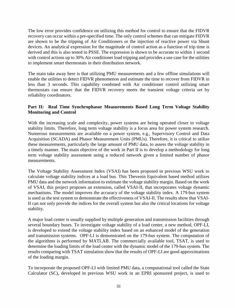
Figure 4.16 Voltage plot of FIDVR with shunt switching as control ........................................... 34

Figure 5.1 Delayed voltage response (top) and the corresponding W-index (bottom) vs the time in samples (60 samples per sec). ....................................................................................................... 35

Figure 5.2 Voltage instability event (top) and the corresponding Lyapunov Exponent (bottom) vs the time in sample (60 samples per sec). ...................................................................................... 35

iv

List of Tables

Table 4.1 Variation of 𝑉𝑉1 and 𝑉𝑉2 with the various load parameters .............................................26

Table 4.2 Error in prediction of 𝑉𝑉1 & 𝑉𝑉2 with change in load composition ..................................27

Table 4.3 Variation of 𝑉𝑉2 with various values of 𝜃𝜃2 .....................................................................28

Table 4.4 Error in 𝑉𝑉2 with change in 𝜃𝜃2 using equation 4.39 .......................................................29

Table 4.5 Power distribution between the various components of the composite load model before and after the fault ...........................................................................................................................30

Table 4.6 Time to recover from FIDVR event in the PSSE simulations by tripping fraction of AC’s........................................................................................................................................................32

Table 4.7 Time to recover from FIDVR event by switching the shunt device ..............................34

1

1. Introduction

1.1 Background

As the bulk electric system operation is moving in to an operation regime where the economics are more important than in the past, the system is operating close to the operating points with more chance of instability. Figure 1.1 provides the classification of power system stability as defined by the IEEE and CIGRE task force.

Figure 1.1 Classification of the various stability phenomenon in power systems [1]

An important type of instability is the short term large disturbance voltage instability that is caused due to increasing penetration of the induction motor and electronic loads. A specific type of short term large disturbance voltage instability is the Fault Induced Delayed Voltage Recovery (FIDVR) and is the main focus of this project. In the FIDVR phenomena, the recovery of the voltage after a disturbance is delayed, resulting in sustained low voltages for several seconds (~15 sec). FIDVR is mainly caused in systems with a moderate amount of single phase induction motor loads (25% ~ 30%). After a large disturbance (fault, etc.), these motors, that are connected to mechanical loads with constant torque, stall and typically draw 5-6 times their nominal current and this leads to the depression of the system voltage for a significant amount of time. The low voltages in the system inherently lead to some load being tripped by protection devices close to the fault. However, even after this, the concern is that the sustained low voltages (>10 s) can lead to cascading events in the system steering towards a blackout. Various methods have been proposed in literature that try to mitigate the FIDVR by ensuring that sufficient VAR resources are present in the system during the planning phase in the system[2, 3, 4]. However, these methods cannot take all the scenarios into account and so a methodology based on the measurements is preferred. This approach is also facilitated by the increasing penetration

2

of the Phasor Measurement Units (PMU) in the transmission system. The PMU can sample the voltage and current phasors at high rates and so the PMU can capture the transition of the system into FIDVR and determine an amount of local control if possible or communicate the control requirements to a control center.

1.2 Report Organization

The report is organized as follows 1. Section 2 describes the Fault Induced Delayed Voltage Recovery phenomenon in detail

and illustrates the various requirements by the reliability coordinators to ensure that this phenomenon is not seen in practice. The load model that can demonstrate FIDVR in software simulations (composite load model) is discussed in detail to illustrate the various components involved in the phenomenon.

2. Section 3 describes the various methods to detect and quantify FIDVR in real time utilizing the PMU voltage measurements at the transmission substation. These methods utilize a reference waveform to quantify the deviation from expected behavior. Several methods with differing properties are introduced and results comparing and contrasting the methods are presented

3. Section 4 presents an analytical framework to analyze the FIDVR phenomenon in terms of the load admittance measures at the transmission substation PMU. The admittance of various components of the composite load model are examined in detail and an analytical expression for the time to recovery from FIDVR in terms of the measured quantities and a few basic properties of the composite load model is derived. Similarly, an expression for the control of air conditioners is also derived in terms of measurements. These expressions are validated on simulation results and are shown to have good agreement with the theoretical expressions.

4. Section 5 describes briefly the OpenPDC methods and presents results from OpenPDC.

3

2. Fault Induced Delayed Voltage Recovery

Short term large disturbance voltage stability is an increasing concern for industry because of the increasing penetration of induction motor and electronically controlled loads. While it is not analytically proven which power system components cause angle and voltage instability, recent work based on an information transfer metric in dynamical systems [5] seems to suggest that the induction motor loads are very much related to voltage instability. The short-term voltage instability is mainly caused by stalling of induction motor loads, and can manifest in the form of fast voltage collapse or delayed voltage recovery. One form of voltage stability is Fault Induced Delayed Voltage Recovery (FIDVR) is the phenomena in which the recovery of the voltage after a disturbance is delayed, resulting in sustained low voltages for several seconds (~15 sec).

2.1 Phenomenon in Power Systems

FIDVR is mainly caused in systems with a moderate amount of single phase induction motor loads (25% ~ 30%). After a large disturbance (fault, etc.), these motors, that are connected to mechanical loads with constant torque, stall and typically draw 5-6 times their nominal current and this leads to the depression of the system voltage for a significant amount of time. The low voltages in the system inherently lead to some load being tripped by protection devices close to the fault. However, even after this, the concern is that the sustained low voltages (>10 s) can lead to cascading events in the system steering towards a blackout. A typical delayed voltage response after a fault along with the various features is shown in Figure 2.1.

Figure 2.1 Conceptual delayed voltage recovery waveform at a bus. Most single phase induction motor are used in residential air-conditioners and so the FIDVR phenomenon has been historically observed in systems where a large number of residential AC’s are operational at the same time (e.g. summer in California or Arizona). Most of these devices do not use Under Voltage protection schemes and are only equipped with the thermal protection with an inverse time-overcurrent feature, delaying the tripping up to 20s. Description of several FIDVR events observed in the field are listed in [6] and almost all of the occur in high residential load areas during a period of high temperature. As an example, Figure 2.2 shows an FIDVR event on a 115kV bus in Southern California on July 24, 2004. The sustained

4

low voltage is likely caused by stalled AC IM’s and the voltage finally recovered to pre-contingency voltage around 25s after the fault. Out of the substation load of 960 MW, 400 MW of load was tripped by protection devices in residential and commercial units to recover the voltage.

Figure 2.2 Recorded delayed voltage recovery waveform at a 115kV bus in Southern California

on July 24, 2004 [6].

Transient Voltage Criteria

To prevent uncontrolled loss of load in the bulk electric system, NERC, WECC and other regulatory bodies have specified transient voltage criteria that utilities and system operators need to satisfy after a fault has been cleared. Figure 2.3 provides a pictorial representation of the WECC criteria and the PJM criteria.

(a) (b)

Figure 2.3 (a) WECC transient voltage criteria [7] (b) Simplified voltage criteria [3]. The WECC transient criteria is defined as the following two requirements [7]

1. Following fault clearing, the voltage shall recover to 80% of the pre-contingency voltage within 20 seconds of the initiating event.

5

2. Following fault clearing and voltage recovery above 80%, voltage at each applicable bulk electric bus serving load shall neither dip below 70% of pre-contingency voltage for more than 30 cycles nor remain below 80% of pre-contingency voltage for more than two seconds.

A simplified voltage criteria is used generally by utilities and the trajectory of the recovering voltage must be above the curve in Figure 2.3(b) where 𝑉𝑉1 = 0.5,𝑉𝑉2 = 0.7 & 𝑉𝑉3 = 0.95 and 𝑇𝑇1 =1 𝑉𝑉,𝑇𝑇2 = 5 𝑉𝑉 & 𝑇𝑇3 = 10 𝑉𝑉. The ERCOT criteria for transient voltage response requires that voltages recover to 0.90 p.u. within 10 seconds of clearing the fault [8]. The utilities ensure that the voltage recovery satisfies the guidelines specified by their regulatory authority during their planning phase and operational phase by either installing VAR devices (STATCOM, SVC, etc.) in critical regions and by ensuring that sufficient dynamic VARS are available during operation.

2.2 Modelling for Simulation – WECC Composite Load Model

In order to enable the utilities and system operators to simulate the FIDVR phenomenon to estimate the amount of VAR support required, a dynamic load model has been developed recently by WECC called as the Dynamic Composite Load Model. The composite model essentially aggregates the various kinds of dynamic loads in the sub-transmission network into several 3-𝜙𝜙 IM (representing high, medium and low inertias) and an aggregate 1-𝜙𝜙 IM (representing the AC loads). Furthermore, the protection schemes that trip a proportion of the loads are also implemented for each of the motor representing the Under Voltage and Under Frequency protections policies. An equivalent feeder is also present that tries to emulate the impact of voltage drop in the distribution system when a large current is drawn. The overall structure of the composite load model is shown in Figure 2.4.

Figure 2.4 Structure of the composite load model [9] This model has 132 parameters and has been implemented by vendors in commercial software such as PSSE, PSLF and PowerWorld. More details along with descriptions of the various parameters can be found in [9]. As part of this project, the CMLD model is studied in detail in

Load Shedding Schemes ZIP Load Aggr.

Large 3-𝜙𝜙 Motor Aggr.

Medium 3-𝜙𝜙 Motor Aggr.

Small 3-𝜙𝜙 Motor Aggr.

All 1-𝜙𝜙 Motors Aggr.

Exponential Load Aggr.

6

order to understand the behavior and simplify the model for control schemes to mitigate FIDVR or to ensure that the FIDVR phenomenon is taken care within the time as specified by the corresponding operator (ERCOT/PJM/WECC)

2.3 Examination of the WECC Composite Load Model

As the composite load model has comparatively large number of parameters and discrete controls compared to a conventional load model, understanding the model and how the various parameters impact the voltage performance is important. Moreover, the model specifications [9] only mention the behavior of most of the components and do not specify the actual equations used. Thus, engineering judgement needs to be made with regards to developing equations for analysis. For this purpose, understanding the 3-phase IM model and the 1-phase IM model along with their protection components are key. These are detailed in the following sub-section.

3-Phase Motor Modelling

A standard way to model, referred to here as the Krauss model, the 3-𝜙𝜙 IM is by an equivalent circuit [10] where the stator and rotor impedances along with the mutual inductances are specified (RA, XA, Xm, R1 & X1). The equations are well studied and it is intuitively understandable as the current in the equivalent circuit directly enables the user to estimate the electric torque. However, as per WECC model specifications, the 3-𝜙𝜙 IM is specified by the transient and sub-transient parameters (Lp, Lpp, Tp0 & Tpp0). The equations for this are not so easily analyzable as they are in the dq frame of reference and so it becomes hard to estimate the impact of load on the electric torque. One way to get around this issue is to convert the sub-transient quantities into corresponding resistance and reactance and analyze the resulting induction motor characteristics (see Appendix 1). To ensure that the dynamics of the load models are comparable, a motor starting study is conducted on the WECC model and the corresponding Krauss model and the resulting speed and torque are plotted in Figure 2.5.

Figure 2.5 Comparison of speed and torque between the Krauss and the WECC model for motor

starting. It can be observed from Figure 2.5 that the WECC model is indeed able to capture the overall dynamics after 0.17s. However, the large oscillations in the torque in the Krauss model till 0.1s are not captured, showing the deficiency of the model. This discrepancy only occurs at low motor

0 0.05 0.1 0.15 0.2 0.25 0.3 0.35

Seconds

0

0.2

0.4

0.6

0.8

1

1.2

Spee

d (p

.u.)

Speed Vs Time

Krauss

WECC

0 0.05 0.1 0.15 0.2 0.25 0.3 0.35

Seconds

-2

-1

0

1

2

3

4

Torq

ue (p

.u.)

Torque Vs Time

Krauss

WECC

7

speed which is not the normal operation of the motor. Even after a fault, the UV relays ensure that the motor operates at a speed close to the rated speed. Thus, this WECC 3-𝜙𝜙 model can replace the Krauss model, assuming that the motor operates close to the rated speed. Another important test is how the variation between the Krauss model and the WECC model changes with the motor inertia. Figure 2.6 plots the steady-state torque-speed curves for the Krauss and the WECC model for high inertia (H=0.5) and low inertia (H=0.1) machines. From the plots, is observed that the maximum torque of the Krauss model is around 10% higher than the WECC model and the difference between the curves is higher for smaller machines.

Figure 2.6 Steady-state torque-speed comparison between the Krauss and the WECC model for

low inertia (left) and high inertia machines (right). Another detail that is often overlooked is the behavior of the motor when a percentage of load is tripped by UV relays. An intuitive method to achieve this is by reducing the mechanical torque by the same percentage to reflect this loss of load. While this indeed reduces, the active power demanded, it does not reduce the reactive power demand. In reality, some of the 3-𝜙𝜙 motors are disconnected and to properly reflect this physical scenario, the resistances of the equivalent circuit must be proportionally increased along with the reduction in the load torque. This ensures a reduction in both the active and reactive power demand.

1-Phase Motor Modelling

The 1-𝜙𝜙 induction motor is the main reason why the FIDVR is observed. The 1-𝜙𝜙 IM model has representations of the AC compressor motor, compressor motor thermal relay, under-voltage relays and contactors. Depending upon the input voltage, the motor operates either in ’running’ or ’stalled’ state. The behavior of the motor as a function of the voltage can is understood based on the power consumption of the motor and Figure 2.7 plots the active and reactive power demand as a function of the voltage for the normal operation and stalled operation.

0 0.2 0.4 0.6 0.8 1 1.2

Speed (p.u)

0

0.5

1

1.5

2

2.5

3

3.5

Torq

ue (p

.u)

0 0.2 0.4 0.6 0.8 1 1.2

Speed (p.u.)

0

0.5

1

1.5

2

2.5

Torq

ue (p

.u.)

Krauss

WECC

8

Figure 2.7 Active power (left) and Reactive power (right) versus the voltage for the normal

operation and stalled operation for the 1 − 𝜙𝜙 induction motor [9]. From Figure 2.7, it can be seen that in the stalled state, the active power demand is 3 times the nominal amount and the reactive demand is 6 times the nominal amount compared to the normal ‘running’ state. This large demand is the reason why the voltage reduces at the substation causing FIDVR. This demand naturally is reduced via thermal protection that takes around 10-15 seconds. More details regarding the 1-phase motor are present in Section 4.1.

3x the Nominal MWat 0.8 p.u.

6x the Nominal MVARat 0.8 p.u.

9

3. Local Voltage Based FIDVR Monitoring

To characterize the performance of the voltage response, WECC has provided guidelines to analyze the voltage performance following a fault. However, the criterion is a pass/fail criterion and do not give any means to quantify the deviation from a normal voltage recovery waveform.

3.1 Lyapunov Exponent

The Lyapunov exponent (LE) is an idea that is adapted from the Ergodic theory of dynamical systems. The maximum Lyapunov exponent is a measure of rate of separation of two trajectories in the system and is used to ascertain the system stability. If the maximum Lyapunov exponent is negative, the trajectories of the system converge to a stable equilibrium. However, if the maximum Lyapunov exponent is positive, the trajectories of the system diverge this suggests a possibly unstable and chaotic system. The equation to compute the Lyapunov exponent of individual buses to estimate the contribution of individual buses to the system stability/instability by using the voltage from a single bus is shown below.

𝜆𝜆𝑖𝑖(𝑘𝑘𝑘𝑘𝑉𝑉) =1

𝑁𝑁𝑘𝑘𝑘𝑘𝑉𝑉� 𝑉𝑉𝑙𝑙𝑙𝑙

||𝑉𝑉𝑖𝑖((𝑘𝑘 + 𝑚𝑚)𝑘𝑘𝑉𝑉) − 𝑉𝑉𝑖𝑖�(𝑘𝑘 + 𝑚𝑚 − 1)𝑘𝑘𝑉𝑉�||||𝑉𝑉𝑖𝑖((𝑚𝑚)𝑘𝑘𝑉𝑉) − 𝑉𝑉𝑖𝑖�(𝑚𝑚− 1)𝑘𝑘𝑉𝑉�||

𝑁𝑁

𝑚𝑚=1

(3.1)

Where 𝑉𝑉𝑖𝑖((𝑚𝑚)𝑘𝑘𝑉𝑉) is the mth sample of voltage measurement at the ith bus and 𝜆𝜆𝑖𝑖 is the Lyapunov exponent at the ith bus. Further details about the LE calculation methodology are in [11]. The bus where the exponent is largest is the main contributor to the instability and control actions taken at this bus will have a large stabilizing impact on the system. The existing formulation of the Lyapunov exponent does not detect FIDVR due to the slow recovery. In order to detect this type of waveforms, a virtual voltage reference is generated at the PMU and the difference between the actual and the reference voltage is used for the calculation of the Lyapunov exponent [12]. The virtual reference is designed such that any voltage waveform above it will be fast recovery and any voltage waveform below it will be delayed recovery. A generic voltage reference which satisfies the above property is shown in 0 with the various parameters whose values can be set depending on the system response. The parameters that decide the waveform can be determined for a given system by doing offline studies. The virtual reference can also be looked as a continuous approximation of the WECC box criterion. The expression for the reference voltage can be written as follows

𝑉𝑉𝑟𝑟𝑒𝑒𝑓𝑓(𝑉𝑉) = �𝑉𝑉0 𝑉𝑉 < 𝑇𝑇0 𝑉𝑉0 + 𝑉𝑉1 ⋅ (1 − 𝑒𝑒�3(𝑇𝑇0−𝑡𝑡)� 𝑇𝑇1⁄ ) 𝑉𝑉 ≥ 𝑇𝑇0

(3.2)

The reference voltage for time 𝑇𝑇0 is flat and is at a low voltage 𝑉𝑉0. This is to allow other protection and control schemes to correct the delayed voltage recovery. Then, the reference voltage rises as an exponential response to settle at (V0 + V1) in a few seconds depending on T0. The reference voltage rises very quickly in the beginning and then the voltage becomes almost flat. The input to the Lyapunov exponent calculation Veff is zero, when reference voltage is below the bus voltage,

10

and is equal to the difference between the reference voltage and the actual voltage response, when the reference voltage is above the actual voltage.

Figure 3.1 A generic voltage reference for applying the Lyapunov exponent to delayed

voltage recovery.

This methodology is applied to response of the IEEE 162 system after a fault of 0.1s. 12 loads are represented by the composite load model in IEEE 162 system with a moderate percentage (30%) of induction motor loads. Fig. 7 shows the voltage response, which is a typical delayed voltage response. The parameter values of the reference voltage waveform are 𝑉𝑉0 = 0.4,𝑇𝑇0 = 1,𝑉𝑉1 =0.55 & 𝑇𝑇1 = 3. The Lyapunov exponents are calculated using both the conventional method and by using the difference between the reference and actual waveform. Results for the case of IEEE 162 bus system with 30% IM load are shown in Fig. 8. It can be seen that the Lyapunov exponent without using the reference is always negative which implies that there is no problem in the system. But there is clearly a delayed voltage recovery problem in the system. This is captured by the Lyapunov exponent going positive by using the reference waveform.

Figure 3.2 The bus voltage (blue) and the voltage reference (green) at a bus in the IEEE 162

system. The LE with and without the reference are plotted on the right. The Lyapunov exponent without using the reference is always negative while it is positive initially by using the reference waveform. The Lyapunov exponent calculated using the reference goes negative after some time. This is due to the fact that the reference has become constant while the actual voltage is slowly recovering. Hence the difference between the two signals will decrease continuously with time – leading to a negative exponent. Thus, utilizing the voltage for determining FIDVR has to be improved.

11

3.2 Kullback- Leibler Divergence

To improve over the LE methodology, instead of using the difference between voltages in a window and comparing them to the initial difference, we will be using the divergence of the voltage waveforms in a time-window. This was inspired on the KL distance proposed to quantify FIDVR for planning of reactive reserves [13]. The divergence is the statistical distance between the probability distribution of the original voltage waveform and the probability distribution of the reference. A pictorial representation of the PDF’s is shown in figure 3.3. This specific probability density function is for the time after the fault (1.1 sec) to the end (5 sec). We use the idea in smaller time-windows to get a real-time implementation.

Figure 3.3 The Voltage time series and the PDF for the voltage series in along with a voltage

reference PDF [13]. The distance between two probability distributions is a well-studied topic in statistics and has been defined so that a positive distance implies a violation of the FIDVR criteria. The KL divergence metric between a probability 𝑝𝑝 and a reference probability 𝑝𝑝𝑟𝑟𝑒𝑒𝑓𝑓 is given by equation 3.3, where 𝑝𝑝𝑖𝑖 & 𝑝𝑝𝑟𝑟𝑒𝑒𝑓𝑓,𝑖𝑖 is the probability in the ith bin of the measured waveform and the reference waveform respectively.

𝐾𝐾𝐾𝐾 = �𝑝𝑝𝑖𝑖 ln�𝑝𝑝𝑖𝑖

𝑝𝑝𝑟𝑟𝑒𝑒𝑓𝑓,𝑖𝑖�

𝑛𝑛

𝑖𝑖=1

(3.3)

The ‘log’ function in the KL expression is a nonlinear term and can cause the divergence to go very high. Also, the division of two probability densities can be impacted by sudden switching actions and unexpected behavior, especially when 𝑝𝑝𝑖𝑖 > 0 and 𝑝𝑝𝑟𝑟𝑒𝑒𝑓𝑓,𝑖𝑖 ~0. This scenario causes the KL index to be negative with a high value due to the division and logarithm function. Thus, the KL index gives a large weight to the bins where the 𝑝𝑝𝑟𝑟𝑒𝑒𝑓𝑓 is close to zero but the 𝑝𝑝 is not close zero. Despite these drawbacks, it can be slightly modified to have a reasonable behavior[4] to analyze the FIDVR event and Figure 3.4 plots the KL index versus time for curves with increasing percentage of IM.

12

Figure 3.4 The voltage at the bus with increasing percentage of induction motor load. The

Moving Divergence based Index of the delayed voltage waveforms. It can be seen from Figure 3.4 that the KL waveforms are well separated and can be used to distinguish between the various responses while it is not so clear just by looking at the voltages. The higher the IM percent, the longer they take to recover to their pre-fault voltage. Also, the response with the least amount of IM has the most negative KL while the response with the largest amount of IM is the least Negative and goes positive for a small amount of time. The slope of the KL index can be used to estimate the time required for the FIDVR to recover, this cannot be done directly on the voltages due to the oscillations. However, there are sharp transitions in the KL index due to the logarithm function and this needs to be improved as well for predictive capabilities.

3.3 Wasserstein Metric

To overcome the challenges with the KL divergence, a smoother metric is needed and for this purpose, the Wasserstein metric is chosen. The Wasserstein metric [14], also called as the earth movers distance, can be understood as the minimal amount of work done to transform a shape of 𝑃𝑃𝑃𝑃𝐹𝐹1 into 𝑃𝑃𝑃𝑃𝐹𝐹2. To determine this distance, an optimization problem needs to be solved and this is not appropriate for real-time applications. However, for 1-D probability density distributions, which is the case we are interested in, the optimal solution has been analytically solved and is shown in Equation 3.4, where 𝐹𝐹1,𝑖𝑖 and 𝐹𝐹2,𝑖𝑖 are the cumulative probability functions of 𝑃𝑃𝑃𝑃𝐹𝐹1 & 𝑃𝑃𝑃𝑃𝐹𝐹2 in bin 𝑖𝑖 respectively.

𝑊𝑊 − 𝑖𝑖𝑖𝑖𝑖𝑖𝑒𝑒𝑖𝑖 = ��𝐹𝐹1,𝑖𝑖 − 𝐹𝐹2,𝑖𝑖�𝑛𝑛

𝑖𝑖=1

(3.4)

Comparing the formulations of the KL divergence and the W-index in equations 3.3 & 3.4, we can make the following observations.

1. The W-index is symmetric as the absolute function is symmetric. The KL index is not symmetric and so is harder to intuitively interpret.

0 5 10 150.1

0.2

0.3

0.4

0.5

0.6

0.7

0.8

0.9

1

1.1

0 5 10 15-1.2

-1

-0.8

-0.6

-0.4

-0.2

0

0.2

13

2. The W-index is incrementally linear, i.e. a small variation in the inputs causes a comparable change in the output value as the absolute function is incrementally linear. This is not the case for the KL divergence due to the logarithm function and the division. A small variation in the inputs can cause an unbounded change in the KL divergence. This property ensures that the W-index is a continuous function with no sudden changes.

3. The W-index is bounded. This is because the cumulative probability functions always lie between 0 and 1, the distance between them can be a maximum of 2. The KL divergence is not bounded again due to the logarithm function. The bounded nature is particularly useful in case of implementation where large results can lead to overflow problems.

To verify that the W-index can indeed be more appropriate in quantifying FIDVR from the voltage waveforms, Figures 3.5 – 3.8 plot the FIDVR response and the W-index.

Figure 3.5 The voltage at the bus with increasing percentage of IM load.

Figure 3.6 The Wasserstein metric based Index of the FIDVR waveforms

Figure 3.7 The Wasserstein metric based Index of the FIDVR waveforms using a

moving time windows of 5s.

Figure 3.8 The Wasserstein metric based Index of the FIDVR waveforms using a

moving time windows of 3s. Similar to the KL plot, it can be seen from Figure 3.6 that the voltages with the least FIDVR have the most negative value of the W-index while the voltages with the FIDVR violating the reference waveform have a W-index that goes to 0 quickly and also becomes positive in the most severe cases. A key difference is that the W-index can differentiate between the waveforms almost from

0 5 10 150.1

0.2

0.3

0.4

0.5

0.6

0.7

0.8

0.9

1

1.1

0 5 10 15-1.4

-1.2

-1

-0.8

-0.6

-0.4

-0.2

0

0.2

0 5 10 15-1.4

-1.2

-1

-0.8

-0.6

-0.4

-0.2

0

0.2

0 5 10 15-1.4

-1.2

-1

-0.8

-0.6

-0.4

-0.2

0

0.2

14

the start while the KL plot only showed the waveforms moving apart after around 2 seconds. The other key difference is that the W-index waveform is much smoother than the KL plot and is due to the continuity property. This enables us to reduce the time window to improve speed of calculations and the memory requirements. Comparing Figure 3.6 with Figures 3.7 and 3.8, the essential information of the deviation from the reference is captured with minimal changes to the waveform. This is not possible with the KL divergence as it is far more non-linear. Thus, the W-index is the best metric to use to quantify FIDVR in real time at a PMU. One of the drawbacks of this approach is that the control mechanisms cannot directly use this information as no information of the reason for the FIDVR is present in the voltage waveforms. To overcome this drawback, we analyzed the admittance of the load during FIDVR and realized that the admittance of the load under FIDVR can have important information that can be used for control. Thus, we propose to utilize the load admittance calculated at the PMU which is observing FIDVR and this is described in the next section.

15

4. Load Admittance Based FIDVR Control

In the previous section, the voltage at the load bus is used to estimate whether the load is experiencing FIDVR and quantify the FIDVR response. This is natural as the WECC and the NERC criteria is in terms of the voltage recovery. However, utilizing the voltage waveform has two issues 1. The voltage waveform has oscillations that are mainly caused due to the behavior of the generator controls and cause problems in the monitoring methods 2. The amount of variation in the voltage between FIDVR waveforms with different amount of IM’s is comparatively small – making it hard to effectively quantify FIDVR Thus, a quantity that that is comparatively smoother than the voltage and which varies more than the voltage is preferable. This quantity should also be closely related to the FIDVR phenomenon as an analytical relation can lead us to predictions on time to recovery. The next sections demonstrate that the load admittance that can be measured using PMU’s satisfies the properties we need and can be very closely linked to the FIDVR phenomenon

4.1 Simplification of the Composite Load Model After Stalling

To understand how the admittance of the composite load can be useful, it is better to represent each load component as an admittance that varies with time. Figure 4.1 represents the structure of the various components of the CMLD model as admittances.

Figure 4.1 Structure of the composite load model with load components as admittances

The voltage at the internal load bus is given by Eq 4.1.

𝑉𝑉𝑖𝑖 = 𝑉𝑉0 ⋅𝑌𝑌𝑓𝑓𝑓𝑓

𝑌𝑌𝑓𝑓𝑓𝑓 + 𝑌𝑌𝐿𝐿;𝑌𝑌𝐿𝐿 = 𝑌𝑌𝑚𝑚𝑚𝑚 + 𝑌𝑌𝑚𝑚𝑚𝑚 + 𝑌𝑌𝑚𝑚𝑚𝑚 + 𝑌𝑌𝑚𝑚𝑚𝑚 + 𝑌𝑌𝑠𝑠 + 𝑌𝑌𝑒𝑒𝑒𝑒 (4.1)

It is observed that after stalling, the variation in the admittance of static loads (𝑌𝑌𝑠𝑠) and the admittance of electronic loads (𝑌𝑌𝑒𝑒𝑒𝑒) do not very much as they are directly reduced as the voltage drops. The admittances of the motors do change significantly during the FIDVR phenomenon and these admittances are analyzed in the sub-sections below.

𝑌𝑌 𝑚𝑚𝑚𝑚

𝑉𝑉0Rest of system 𝑌𝑌𝑓𝑓𝑓𝑓

𝑌𝑌 𝑚𝑚𝑚𝑚

𝑌𝑌 𝑚𝑚𝑚𝑚

𝑌𝑌 𝑚𝑚𝑚𝑚

𝑌𝑌 𝑠𝑠 𝑌𝑌 𝑒𝑒𝑒𝑒

𝑉𝑉𝑖𝑖

16

3-Phase Motor Admittance Analysis

The equivalent circuit of the 3-phase motor is shown in Figure 4.2 and is used to analyze how the motor admittance varies during the stalling condition. The equivalent impedance of the motor is a function of the slip (s) and is shown in equation 4.2.

Figure 4.2 Simplified equivalent circuit of a 3-phase induction motor [10]

𝑍𝑍𝑚𝑚 = 𝑅𝑅𝑠𝑠 + 𝑗𝑗 ⋅ 𝑋𝑋𝑠𝑠 +�𝑅𝑅𝑟𝑟𝑉𝑉 + 𝑗𝑗 ⋅ 𝑋𝑋𝑟𝑟� (𝑗𝑗 ⋅ 𝑋𝑋𝑚𝑚)

�𝑅𝑅𝑟𝑟𝑉𝑉 + 𝑗𝑗(𝑋𝑋𝑟𝑟 + 𝑋𝑋𝑚𝑚)� (4.2)

As per the WECC CMLD document [9], the 3-Phase motors are all equipped with appropriate UV relays that ensure that load is reduced as the voltage drops. This is pictorially represented in Figure 4.3 with the load torque proportional to the square of the rotation speed.

Figure 4.3 The variation in motor speed when the voltage and the load are reduced

These features ensure that the rotor speed of the 3-Phase motors is close to the rated speed and so the slip (s) varies in a tight range (around 0.04 at nominal operation to an extreme of 0.1 at the low voltage condition). Utilizing this range of slip, the admittance of the load motors is now analyzed below in equations 4.3 to 4.11.

𝑌𝑌𝑚𝑚(𝑉𝑉) =𝑅𝑅𝑟𝑟/𝑉𝑉 + 𝑗𝑗(𝑋𝑋𝑟𝑟 + 𝑋𝑋𝑚𝑚)

(𝑅𝑅𝑟𝑟/𝑉𝑉 + 𝑗𝑗 ⋅ 𝑋𝑋𝑟𝑟)(𝑗𝑗 ⋅ 𝑋𝑋𝑚𝑚) + �𝑅𝑅𝑟𝑟/𝑉𝑉 + 𝑗𝑗(𝑋𝑋𝑚𝑚 + 𝑋𝑋𝑟𝑟)�(𝑅𝑅𝑠𝑠 + 𝑗𝑗 ⋅ 𝑋𝑋𝑠𝑠) (4.3)

17

Using the fact that for practical motors, 𝑋𝑋𝑚𝑚 ≫ 𝑋𝑋𝑟𝑟 & 𝑋𝑋𝑠𝑠 ≫ 𝑅𝑅𝑠𝑠, it is simplified to

𝑌𝑌𝑚𝑚(𝑉𝑉) ≈𝑅𝑅𝑟𝑟 + 𝑗𝑗 ⋅ 𝑋𝑋𝑚𝑚 ⋅ 𝑉𝑉

(𝑅𝑅𝑟𝑟 + 𝑗𝑗 ⋅ 𝑋𝑋𝑟𝑟 ⋅ 𝑉𝑉)(𝑗𝑗 ⋅ 𝑋𝑋𝑚𝑚) + (𝑅𝑅𝑟𝑟 + 𝑗𝑗 ⋅ 𝑋𝑋𝑚𝑚 ⋅ 𝑉𝑉)(𝑗𝑗 ⋅ 𝑋𝑋𝑠𝑠) (4.4)

𝑌𝑌𝑚𝑚(𝑉𝑉) ≈𝑅𝑅𝑟𝑟 + 𝑗𝑗 ⋅ 𝑋𝑋𝑚𝑚 ⋅ 𝑉𝑉

�𝑅𝑅𝑟𝑟 ⋅ (𝑗𝑗 ⋅ 𝑋𝑋𝑚𝑚 + 𝑗𝑗 ⋅ 𝑋𝑋𝑠𝑠)� + (𝑗𝑗 ⋅ 𝑋𝑋𝑚𝑚 ⋅ 𝑉𝑉)(𝑗𝑗 ⋅ 𝑋𝑋𝑠𝑠 + 𝑗𝑗 ⋅ 𝑋𝑋𝑟𝑟) (4.5)

Using the fact that for practical motors, 𝑋𝑋𝑚𝑚 ≫ 𝑋𝑋𝑠𝑠, it is simplified to

𝑌𝑌𝑚𝑚(𝑉𝑉) ≈ �1

𝑗𝑗 ⋅ 𝑋𝑋𝑚𝑚��1 +

𝑗𝑗(𝑋𝑋𝑚𝑚 − 𝑋𝑋𝑠𝑠 − 𝑋𝑋𝑟𝑟)𝑅𝑅𝑟𝑟/𝑉𝑉 + (𝑗𝑗 ⋅ 𝑋𝑋𝑠𝑠 + 𝑗𝑗 ⋅ 𝑋𝑋𝑟𝑟)� (4.6)

Suppose only a fraction (𝑓𝑓𝑢𝑢𝑢𝑢 < 1) of the motors are operating during FIDVR (i.e. (1 − 𝑓𝑓𝑢𝑢𝑢𝑢) fraction is tripped), then the admittance is also scaled by 𝑓𝑓𝑢𝑢𝑢𝑢. Thus, the expression for the admittance during FIDVR is given by

𝑌𝑌𝑚𝑚(𝑉𝑉) = �𝑓𝑓𝑢𝑢𝑢𝑢𝑗𝑗 ⋅ 𝑋𝑋𝑚𝑚

��1 +𝑗𝑗(𝑋𝑋𝑚𝑚 − 𝑋𝑋𝑠𝑠 − 𝑋𝑋𝑟𝑟)

𝑅𝑅𝑟𝑟/𝑉𝑉 + (𝑗𝑗 ⋅ 𝑋𝑋𝑠𝑠 + 𝑗𝑗 ⋅ 𝑋𝑋𝑟𝑟)� (4.7)

Suppose the slip of the motor is 𝑉𝑉0 at nominal operating point and it is 𝑉𝑉1 during the FIDVR, then the ratio between the two admittances is given by Eq 4.8.

𝑌𝑌𝑚𝑚(𝑉𝑉1)𝑌𝑌𝑚𝑚(𝑉𝑉0)

= 𝑓𝑓𝑢𝑢𝑢𝑢 ⋅𝑅𝑅𝑟𝑟 + 𝑗𝑗 ⋅ 𝑋𝑋𝑚𝑚 ⋅ 𝑉𝑉1

𝑅𝑅𝑟𝑟 + (𝑗𝑗 ⋅ 𝑋𝑋𝑠𝑠 + 𝑗𝑗 ⋅ 𝑋𝑋𝑟𝑟) ⋅ 𝑉𝑉1⋅𝑅𝑅𝑟𝑟 + (𝑗𝑗 ⋅ 𝑋𝑋𝑠𝑠 + 𝑗𝑗 ⋅ 𝑋𝑋𝑟𝑟) ⋅ 𝑉𝑉0

𝑅𝑅𝑟𝑟 + 𝑗𝑗 ⋅ 𝑋𝑋𝑚𝑚 ⋅ 𝑉𝑉0 (4.8)

𝑌𝑌𝑚𝑚(𝑉𝑉1)𝑌𝑌𝑚𝑚(𝑉𝑉0) = 𝑓𝑓𝑢𝑢𝑢𝑢 ⋅

𝑅𝑅𝑟𝑟2 − 𝑋𝑋𝑚𝑚(𝑋𝑋𝑠𝑠 + 𝑋𝑋𝑟𝑟) ⋅ 𝑉𝑉1 ⋅ 𝑉𝑉0 + 𝑗𝑗 ⋅ 𝑅𝑅𝑟𝑟 ⋅ (𝑋𝑋𝑚𝑚 ⋅ 𝑉𝑉1 + (𝑋𝑋𝑠𝑠 + 𝑋𝑋𝑟𝑟) ⋅ 𝑉𝑉0)𝑅𝑅𝑟𝑟2 − 𝑋𝑋𝑚𝑚(𝑋𝑋𝑠𝑠 + 𝑋𝑋𝑟𝑟) ⋅ 𝑉𝑉1 ⋅ 𝑉𝑉0 + 𝑗𝑗 ⋅ 𝑅𝑅𝑟𝑟 ⋅ (𝑋𝑋𝑚𝑚 ⋅ 𝑉𝑉0 + (𝑋𝑋𝑠𝑠 + 𝑋𝑋𝑟𝑟) ⋅ 𝑉𝑉1) (4.9)

Let 𝑅𝑅𝑟𝑟 = 𝜂𝜂1 ⋅ 𝑉𝑉0 & 𝑉𝑉1 = 𝜂𝜂2 ⋅ 𝑉𝑉0 . Utilizing the fact that 𝑋𝑋𝑚𝑚 ≫ (𝑋𝑋𝑠𝑠 + 𝑋𝑋𝑟𝑟) , Eq 4.9 can be simplified as

𝑌𝑌𝑚𝑚(𝑉𝑉1)𝑌𝑌𝑚𝑚(𝑉𝑉0) ≈ 𝑓𝑓𝑢𝑢𝑢𝑢 �1 +

𝑗𝑗(𝜂𝜂2 − 𝜂𝜂1) ⋅ (𝑋𝑋𝑚𝑚)1 − 𝑋𝑋𝑚𝑚(𝑋𝑋𝑠𝑠 + 𝑋𝑋𝑟𝑟) ⋅ 𝜂𝜂2 ⋅ 𝜂𝜂1 + 𝑗𝑗(𝑋𝑋𝑚𝑚 ⋅ 𝜂𝜂1 + (𝑋𝑋𝑠𝑠 + 𝑋𝑋𝑟𝑟) ⋅ 𝜂𝜂2)� (4.10)

As it was discussed from Figure 4.3 , 1.5 < 𝜂𝜂2 < 3. Also, in practical motors, 1/3 < 𝜂𝜂1 < 2 & 𝑓𝑓𝑢𝑢𝑢𝑢 ≈ 0.6. For the default motor parameters in WECC, the ratio satisfies equation 4.11.

18

1 < �𝑌𝑌𝑚𝑚(𝑉𝑉1)𝑌𝑌𝑚𝑚(𝑉𝑉0)� < 3.5 (4.11)

Thus, the admittance of the 3-Phase motors during the FIDVR phenomenon can be at most around 3.5 times the nominal admittance.

1-Phase Motor Admittance Analysis

The stalling of the 1-phase motors is the main cause of the FIDVR phenomenon. Due to this, the 1-phase motors that remain connected during the FIDVR phenomenon are represented by a constant impedance. This impedance is much smaller than the nominal impedance of the 1-phase motor in normal operation. Since we are inspecting at all the elements in the CMLD model as admittances, we can conclude that the FIDVR admittance of the 1-phase motor is several times the nominal admittance. From Figure 2.7, it can be deduced that for the WECC default parameters, the FIDVR conductance is 5 times the nominal conductance and the FIDVR susceptance is 10 times the nominal susceptance. This large increase in the conductance and susceptance can be used to characterize the 1-phase motor. Another important characteristic of the 1-phase motor are the various control schemes. Just as the 3-phase motor has UV protection devices to reduce the load when the voltage drops, the 1-phase motor also has UV protection, but the percentage of load that has this protection is very small (~5%-10% of the 1-phase motors). On top of the UV relays, there are also contactors that reduce the load below 0.65 p.u. voltage. However, the main protection device is the thermal protection logic that is present in all the 1-phase motors. The thermal tripping logic is shown in Figure 4.4, where 𝑓𝑓𝑇𝑇𝑇𝑇 is the fraction of 1-phase motors connected, 𝜃𝜃 is the internal motor temperature, 𝑇𝑇𝑡𝑡ℎ is the thermal delay time constant in the protection logic with the thermal power dissipated in the motor given by 𝑉𝑉2 ⋅ 𝐺𝐺𝑠𝑠𝑡𝑡𝑠𝑠𝑒𝑒𝑒𝑒.

Figure 4.4 The thermal protection logic implemented in the composite load model

The admittance of the 1-phase motor during FIDVR is given by equation 4.12.

𝑌𝑌𝑚𝑚𝑚𝑚 = 𝑓𝑓𝑈𝑈𝑈𝑈 ⋅ 𝑓𝑓𝑇𝑇𝑇𝑇(𝐺𝐺𝑠𝑠𝑡𝑡𝑠𝑠𝑒𝑒𝑒𝑒 + 𝑗𝑗 ⋅ 𝐵𝐵𝑠𝑠𝑡𝑡𝑠𝑠𝑒𝑒𝑒𝑒) (4.12)

As the admittance of the 1-phase motor is dependent on 𝑓𝑓𝑡𝑡ℎ, it is important to analyse the behavior of the thermal trip logic. After a fault that initiates the FIDVR event, the thermal loss in the motor increases suddenly and the thermal trip logic is initiated. The thermal delay block simulates the time delay of the rise in the temperature of the motor coil. This estimated motor coil temperature

θ1T θ2T

θ

fTH1

0

θ fTH

connected

Motor

mperature𝜃𝜃

19

is what determines the fraction of 1-phase motor connected to the grid. The fraction of 1-phase motors connected is determined by the 𝜃𝜃1 & 𝜃𝜃2 parameters. A temperature that is lesser than 𝜃𝜃1 does not change the admittance and keeps the fraction connected (𝑓𝑓𝑇𝑇𝑇𝑇) as 1. When the motor temperature is between 𝜃𝜃1 and 𝜃𝜃2, the 𝑓𝑓𝑇𝑇𝑇𝑇 is reduced linearly from 1 to 0. And when the temperature is reaches 𝜃𝜃2, there are no more 1-phase motors connected to the grid. The parameters 𝜃𝜃1 and 𝜃𝜃2 are key in determining the time that the FIDVR event persists and analytically deriving the time taken for the temperature to reach 𝜃𝜃2 is a way to estimate this time.

4.1.2.1 Derivation of time for thermal tripping to initiate (t1)

Since the behavior of the system is different before and after 𝜃𝜃1, we first determine the time taken for the motor temperature to rise to 𝜃𝜃1. Since 𝜃𝜃 is the output of a time delayed block with a delay 𝑇𝑇𝑇𝑇𝑇𝑇 and the thermal power rises suddenly at stalling, we can use the step input formula to determine the variation of 𝜃𝜃 as a function of time. Let the thermal power be denoted by 𝑃𝑃𝑡𝑡ℎ and let 𝑉𝑉1 be the time taken to reach a temperature of 𝜃𝜃1. Equations 4.13 to 4.16 follow from the definitions and using the first term in the power series expansion ln(1 − 𝑖𝑖) ≈ −𝑖𝑖.

𝑃𝑃𝑡𝑡ℎ = 𝑉𝑉𝑖𝑖2 ⋅ 𝐺𝐺𝑠𝑠𝑡𝑡𝑠𝑠𝑒𝑒𝑒𝑒 = 𝑉𝑉02 ⋅�𝑌𝑌𝑓𝑓𝑓𝑓�

2

�𝑌𝑌𝑓𝑓𝑓𝑓 + 𝑌𝑌𝐿𝐿�2 ⋅ 𝐺𝐺𝑠𝑠𝑡𝑡𝑠𝑠𝑒𝑒𝑒𝑒 (4.13)

𝜃𝜃1 = 𝑃𝑃𝑡𝑡ℎ�1 − 𝑒𝑒(−𝑡𝑡1/𝑇𝑇𝑡𝑡ℎ)� (4.14)

𝑉𝑉1 = −𝑇𝑇𝑡𝑡ℎ ⋅ ln(1 − 𝜃𝜃1/𝑃𝑃𝑡𝑡ℎ) ≈ 𝑇𝑇𝑡𝑡ℎ ⋅ 𝜃𝜃1/𝑃𝑃𝑡𝑡ℎ (4.15)

𝑉𝑉1 ≈𝑇𝑇𝑡𝑡ℎ ⋅ 𝜃𝜃1𝑉𝑉02 ⋅ 𝐺𝐺𝑠𝑠𝑡𝑡𝑠𝑠𝑒𝑒𝑒𝑒

⋅ �1 +𝑌𝑌𝐿𝐿𝑌𝑌𝑓𝑓𝑓𝑓

�2

(4.16)

Using the fact that the 𝑌𝑌𝐿𝐿 is mostly made up of the admittance of 𝑌𝑌𝑚𝑚𝑚𝑚 = 𝐵𝐵𝑠𝑠𝑡𝑡𝑠𝑠𝑒𝑒𝑒𝑒 + 𝑗𝑗 ⋅ 𝐺𝐺𝑠𝑠𝑡𝑡𝑠𝑠𝑒𝑒𝑒𝑒, with 𝐵𝐵𝑠𝑠𝑡𝑡𝑠𝑠𝑒𝑒𝑒𝑒 = 𝐺𝐺𝑠𝑠𝑡𝑡𝑠𝑠𝑒𝑒𝑒𝑒, we can simplify the expression to

𝑉𝑉1 ≈𝑇𝑇𝑡𝑡ℎ ⋅ 𝜃𝜃1𝑉𝑉02

⋅ �1

𝐺𝐺𝑠𝑠𝑡𝑡𝑠𝑠𝑒𝑒𝑒𝑒+

2𝑌𝑌𝑓𝑓𝑓𝑓

+2 ⋅ 𝐵𝐵𝑠𝑠𝑡𝑡𝑠𝑠𝑒𝑒𝑒𝑒𝑌𝑌𝑓𝑓𝑓𝑓2

� ≈2 ⋅ 𝑇𝑇𝑡𝑡ℎ ⋅ 𝜃𝜃1 ⋅ 𝐵𝐵0

𝑉𝑉02 ⋅ 𝑌𝑌𝑓𝑓𝑓𝑓2 (4.17)

Here 𝐵𝐵0 is the susceptance seen by the high voltage transmission bus before the feeder. Hence, the time taken for the thermal tripping to begin is proportional to the initial susceptance 𝐵𝐵0, Thermal time constant 𝑇𝑇𝑇𝑇𝑇𝑇, Temperature setting 𝜃𝜃1 and is inversely proportional to the initial post-contingency high voltage transmission voltage 𝑉𝑉0 square and the feeder impedance squared.

20

4.1.2.2 Derivation of time for thermal tripping to terminate (t2)

Now that the behavior of the system is understood before 𝜃𝜃1, we can determine the time taken for the motor temperature to rise to 𝜃𝜃2 from 𝜃𝜃1 by understanding the linear reduction in the thermal trip fraction 𝑓𝑓𝑇𝑇𝑇𝑇. Equations 4.18 to 4.22 follow from the definitions and by utilizing the first order differential equation relation between the thermal power (𝑃𝑃𝑇𝑇𝑇𝑇) and the motor temperature (𝜃𝜃).

�̇�𝜃 =1𝑇𝑇𝑇𝑇ℎ

(𝑃𝑃𝑇𝑇𝑇𝑇 − 𝜃𝜃) (4.18)

𝑓𝑓𝑇𝑇𝑇𝑇 = 1 − �𝜃𝜃 − 𝜃𝜃1𝜃𝜃2 − 𝜃𝜃1

� ⇒ 𝜃𝜃 = (𝜃𝜃2 − 𝜃𝜃1) ⋅ (1 − 𝑓𝑓𝑇𝑇𝑇𝑇) + 𝜃𝜃1 (4.19)

𝑃𝑃𝑇𝑇𝑇𝑇 = 𝑉𝑉𝑖𝑖2 ⋅ 𝐺𝐺𝑠𝑠𝑡𝑡𝑠𝑠𝑒𝑒𝑒𝑒 = 𝑉𝑉02 ⋅�𝑌𝑌𝑓𝑓𝑓𝑓�

2

�𝑌𝑌𝑓𝑓𝑓𝑓 + 𝑓𝑓𝑇𝑇𝑇𝑇 ⋅ 𝑌𝑌𝐿𝐿�2 ⋅ 𝐺𝐺𝑠𝑠𝑡𝑡𝑠𝑠𝑒𝑒𝑒𝑒 (4.20)

Utilizing the above expressions, a differential equation in terms of the fraction

𝑓𝑓𝑇𝑇𝑇𝑇̇ = −�̇�𝜃

(𝜃𝜃2 − 𝜃𝜃1) (4.21)

𝑓𝑓𝑇𝑇�̇�𝑇 =1

𝑇𝑇𝑇𝑇𝑇𝑇(𝜃𝜃2 − 𝜃𝜃1)�𝜃𝜃2 −(𝜃𝜃2 − 𝜃𝜃1) ⋅ 𝑓𝑓𝑇𝑇𝑇𝑇 −

𝑉𝑉02 ⋅ 𝐺𝐺𝑠𝑠𝑡𝑡𝑠𝑠𝑒𝑒𝑒𝑒�1 + 𝑓𝑓𝑇𝑇𝑇𝑇 ⋅ (𝑌𝑌𝐿𝐿/𝑌𝑌𝑓𝑓𝑓𝑓)�

2� (4.22)

The power series expansion for 1(1+𝑥𝑥)2 is Σ(𝑖𝑖 + 1)𝑖𝑖𝑛𝑛. This is valid as 𝑓𝑓𝑇𝑇𝑇𝑇 ≤ 1 and in practice the

ratio 𝑌𝑌𝐿𝐿/𝑌𝑌𝑓𝑓𝑓𝑓 < 0.5. Let 𝛾𝛾 = 1/𝑇𝑇𝑇𝑇𝑇𝑇(𝜃𝜃2 − 𝜃𝜃1). Considering only the first 2 terms in the power series expansion, the equation can be simplified as follows.

𝑓𝑓𝑇𝑇𝑇𝑇̇ = γ�𝜃𝜃2 − (𝜃𝜃2 − 𝜃𝜃1) ⋅ 𝑓𝑓𝑇𝑇𝑇𝑇 − 𝑉𝑉02 ⋅ 𝐺𝐺𝑠𝑠𝑡𝑡𝑠𝑠𝑒𝑒𝑒𝑒 ⋅ �1 − 2 ⋅ �𝑓𝑓𝑇𝑇𝑇𝑇 ⋅ 𝑌𝑌𝐿𝐿𝑌𝑌𝑓𝑓𝑓𝑓

��� (4.23)

𝑓𝑓𝑇𝑇�̇�𝑇 = γ�(𝜃𝜃2 − 𝑉𝑉02 ⋅ 𝐺𝐺𝑠𝑠𝑡𝑡𝑠𝑠𝑒𝑒𝑒𝑒) − �(𝜃𝜃2 − 𝜃𝜃1) −2 ⋅ 𝑉𝑉02 ⋅ 𝐺𝐺𝑠𝑠𝑡𝑡𝑠𝑠𝑒𝑒𝑒𝑒 ⋅ 𝑌𝑌𝐿𝐿

𝑌𝑌𝑓𝑓𝑓𝑓� ⋅ 𝑓𝑓𝑇𝑇𝑇𝑇� (4.24)

Using the fact that 𝑉𝑉02 ⋅ 𝐺𝐺𝑠𝑠𝑡𝑡𝑠𝑠𝑒𝑒𝑒𝑒 > 𝜃𝜃2, (𝜃𝜃2 − 𝜃𝜃1) > 0 and 𝑌𝑌𝐿𝐿

𝑌𝑌𝑓𝑓𝑓𝑓< 0.5, we get

𝑓𝑓𝑇𝑇�̇�𝑇 = 𝛼𝛼 + 𝛽𝛽 ⋅ 𝑓𝑓𝑇𝑇𝑇𝑇 (4.25)

21

𝛼𝛼 =(𝜃𝜃2 − 𝑉𝑉02 ⋅ 𝐺𝐺𝑠𝑠𝑡𝑡𝑠𝑠𝑒𝑒𝑒𝑒)𝑇𝑇𝑇𝑇𝑇𝑇(𝜃𝜃2 − 𝜃𝜃1) < 0 (4.26)

𝛽𝛽 = −�(𝜃𝜃2 − 𝜃𝜃1) −2 ⋅ 𝑉𝑉02 ⋅ 𝐺𝐺𝑠𝑠𝑡𝑡𝑠𝑠𝑒𝑒𝑒𝑒 ⋅ 𝑌𝑌𝐿𝐿

𝑌𝑌𝑓𝑓𝑓𝑓� < 0 (4.27)

Since both the coefficients are negative, the fraction 𝑓𝑓𝑇𝑇𝑇𝑇 monotonically decreases. The initial value of 𝑓𝑓𝑇𝑇𝑇𝑇 is 1 and as 𝑓𝑓𝑇𝑇𝑇𝑇 is decreasing, the fraction reaches 0 at which time the equations do not valid anymore. Since this is a small range, an approximation that the slope of 𝑓𝑓𝑇𝑇ℎ is constant is reasonable. To determine this slope, the average value of 𝑓𝑓𝑇𝑇𝑇𝑇̇ at 𝑓𝑓𝑇𝑇𝑇𝑇 = 1 and 𝑓𝑓𝑇𝑇ℎ = 0 can be used. In the derivation above, we have assumed that 𝑉𝑉0 is constant. However, the voltage at the transmission bus rises to around 1.0 p.u. when the fraction 𝑓𝑓𝑇𝑇ℎ = 0. Hence the average slope is given by equation 4.28.

𝑓𝑓�̇�𝑇𝑇𝑇−𝑚𝑚𝑒𝑒𝑠𝑠𝑛𝑛 =1

2 ⋅ 𝑇𝑇𝑇𝑇𝑇𝑇(𝜃𝜃2 − 𝜃𝜃1)�𝜃𝜃1 − 𝑉𝑉02 ⋅ 𝐺𝐺𝑠𝑠𝑡𝑡𝑠𝑠𝑒𝑒𝑒𝑒 �1 − 2 ⋅𝑌𝑌𝐿𝐿𝑌𝑌𝑓𝑓𝑓𝑓

� + 𝜃𝜃2 − 𝐺𝐺𝑠𝑠𝑡𝑡𝑠𝑠𝑒𝑒𝑒𝑒� (4.28)

𝑓𝑓�̇�𝑇𝑇𝑇−𝑚𝑚𝑒𝑒𝑠𝑠𝑛𝑛 =1

2 ⋅ 𝑇𝑇𝑇𝑇𝑇𝑇(𝜃𝜃2 − 𝜃𝜃1)�𝜃𝜃1 + 𝜃𝜃2 − 𝐺𝐺𝑠𝑠𝑡𝑡𝑠𝑠𝑒𝑒𝑒𝑒 �1 + 𝑉𝑉02 −2 ⋅ 𝑉𝑉02 ⋅ 𝑌𝑌𝐿𝐿

𝑌𝑌𝑓𝑓𝑓𝑓�� (4.29)

Utilizing the identity Σ(𝑖𝑖 + 1)𝑖𝑖𝑛𝑛 = 1

(1+𝑥𝑥)2 , the mean slope can be written as

𝑓𝑓�̇�𝑇𝑇𝑇−𝑚𝑚𝑒𝑒𝑠𝑠𝑛𝑛 =1

2 ⋅ 𝑇𝑇𝑇𝑇𝑇𝑇(𝜃𝜃2 − 𝜃𝜃1)�𝜃𝜃1 + 𝜃𝜃2 − 𝐺𝐺𝑠𝑠𝑡𝑡𝑠𝑠𝑒𝑒𝑒𝑒 �1 +𝑉𝑉02

�1 + (𝑌𝑌𝐿𝐿/𝑌𝑌𝑓𝑓𝑓𝑓)�2�� (4.30)

In practice, the 𝐺𝐺𝑠𝑠𝑡𝑡𝑠𝑠𝑒𝑒𝑒𝑒 ≫ (𝜃𝜃1 + 𝜃𝜃2) and so we can approximate the slope as

𝑓𝑓�̇�𝑇𝑇𝑇−𝑚𝑚𝑒𝑒𝑠𝑠𝑛𝑛 =−𝐺𝐺𝑠𝑠𝑡𝑡𝑠𝑠𝑒𝑒𝑒𝑒

2 ⋅ 𝑇𝑇𝑇𝑇𝑇𝑇(𝜃𝜃2 − 𝜃𝜃1)�1 +𝑉𝑉02

�1 + (𝑌𝑌𝐿𝐿/𝑌𝑌𝑓𝑓𝑓𝑓)�2� (4.31)

Since 𝐺𝐺𝑠𝑠𝑡𝑡𝑠𝑠𝑒𝑒𝑒𝑒 and 𝐵𝐵𝑠𝑠𝑡𝑡𝑠𝑠𝑒𝑒𝑒𝑒 are same and it is more valid to approximate 𝐵𝐵𝑠𝑠𝑡𝑡𝑠𝑠𝑒𝑒𝑒𝑒 with 𝐵𝐵0, we arrive at the final expression for the mean slope of the thermal trip fraction.

𝑓𝑓�̇�𝑇𝑇𝑇−𝑚𝑚𝑒𝑒𝑠𝑠𝑛𝑛 =−𝐵𝐵0

2 ⋅ 𝑇𝑇𝑇𝑇𝑇𝑇(𝜃𝜃2 − 𝜃𝜃1)�1 +𝑉𝑉02

�1 + (𝑌𝑌𝐿𝐿/𝑌𝑌𝑓𝑓𝑓𝑓)�2� (4.32)

22

Thus, from expression above, the slope of the susceptance during the FIDVR event is inversely proportional to the Thermal delay (𝑇𝑇𝑇𝑇𝑇𝑇), the difference (𝜃𝜃2 − 𝜃𝜃1) and directly proportional to the initial observed susceptance during the FIDVR event (𝐵𝐵0). In the above derivations for 𝑉𝑉1& 𝑉𝑉2, several approximations and simplifying assumptions were made. It is important to validate that 𝑉𝑉1& 𝑉𝑉2 do indeed vary as simple functions of the measured susceptance 𝐵𝐵0. The validation of the variation of 𝑉𝑉1& 𝑉𝑉2 as a function of 𝑇𝑇𝑇𝑇𝑇𝑇 , θ1 ,θ2 & B0 is done on PSSE simulations in the next sub-section.

4.2 Validation Results from PSSE Simulations

The IEEE 162 bus system is used to test the claims from the previous section regarding the variation of the time to recover from FIDVR utilizing the effective susceptance of the composite load. A fault is applied at 1 sec lasting 3 cycles and is cleared by opening a line. The information of the location of the composite load model and other system details are in [3]. The simulation outputs the voltage and the active and reactive powers observed at the transmission substation and the following equations are used to determine the susceptance and the conductance at every time step. These calculations are straightforward and can be implemented easily at the PMU in real-time when the FIDVR occurs.

𝑌𝑌0 = 𝐺𝐺0 + 𝑗𝑗𝐵𝐵0 (4.33)

𝑃𝑃𝑡𝑡𝑟𝑟𝑠𝑠𝑛𝑛𝑠𝑠 = 𝑉𝑉02 ⋅ 𝐺𝐺0 ⇒ 𝐺𝐺0 = 𝑃𝑃𝑡𝑡𝑟𝑟𝑠𝑠𝑛𝑛𝑠𝑠/𝑉𝑉02 (4.34)

𝑄𝑄𝑡𝑡𝑟𝑟𝑠𝑠𝑛𝑛𝑠𝑠 = 𝑉𝑉02 ⋅ 𝐵𝐵0 ⇒ 𝐵𝐵0 = 𝑄𝑄𝑡𝑡𝑟𝑟𝑠𝑠𝑛𝑛𝑠𝑠/𝑉𝑉02 (4.35)

The stall impedance is kept constant at 0.1+j0.1for all the results in this section. The load fractions of the various components and the parameters of the thermal trip logic are varied to see how they match up to the expectations. Figures 4.5 and 4.6 plot the voltage and susceptance for a normal voltage recovery and a delayed voltage recovery after a fault.

23

Figure 4.5 Voltage plots of the normal and delayed voltage recovery after fault clearing

Figure 4.6 Susceptance plot of the normal and delayed voltage recovery scenarios

It can be observed from the plots that the oscillations present in the voltage wave form are not present in the susceptance plot. In case of a normal recovery, the susceptance very quickly returns to the pre-contingency susceptance while in case of the delayed recovery, there is large delay for the susceptance to return to the pre-contingency levels and it actually settles to a lower value as some of the load is tripped by protection logic during the FIDVR event. The voltage has oscillations after the clearing of the fault while the oscillations in the susceptance are comparatively smaller. The susceptance remains almost flat for 𝑉𝑉1 seconds and then reduces linearly to the pre-contingency level in 𝑉𝑉2 seconds. This behavior is what was modelled in the

24

previous section and the results seem to validate the analysis. There are small deviations from what is ideally expected in the susceptance waveform

1. Small step variations in the susceptance around 4 seconds 2. Small drop in the susceptance around 12 seconds

Both variations are due to the switching of the UV trip circuit of the 3-phase motors and the electronic loads. Notice that their impact on the overall behavior of the susceptance is negligible. To verify the claims made in section 4.1, several simulation runs in PSSE are conducted with varying the fractions of motors A, B, C, D, Static Load and Electronic load. In the interest of space, results of the following cases are discussed further.

1. Case-0: 𝑓𝑓𝑚𝑚𝑚𝑚 = 0.1,𝑓𝑓𝑚𝑚𝑚𝑚 = 0.1,𝑓𝑓𝑚𝑚𝑚𝑚 = 0.0

2. Case-1: 𝑓𝑓𝑚𝑚𝑚𝑚 = 0.1,𝑓𝑓𝑚𝑚𝑚𝑚 = 0.1,𝑓𝑓𝑚𝑚𝑚𝑚 = 0.2

3. Case-2: 𝑓𝑓𝑚𝑚𝑚𝑚 = 0.1,𝑓𝑓𝑚𝑚𝑚𝑚 = 0.1,𝑓𝑓𝑚𝑚𝑚𝑚 = 0.35

4. Case-3: 𝑓𝑓𝑚𝑚𝑚𝑚 = 0.1,𝑓𝑓𝑚𝑚𝑚𝑚 = 0.2,𝑓𝑓𝑚𝑚𝑚𝑚 = 0.35

5. Case-4: 𝑓𝑓𝑚𝑚𝑚𝑚 = 0.2,𝑓𝑓𝑚𝑚𝑚𝑚 = 0.2,𝑓𝑓𝑚𝑚𝑚𝑚 = 0.35 The voltage and the susceptance for these cases after a fault is plotted in Figures 4.6 & 4.7.

Figure 4.7 Voltage plot for different proportions of motors A, B &D

25

Figure 4.8 Susceptance plot for different proportions of motors A, B &D

The following important observations can be made from the voltage and susceptance plots for the various scenarios

1. The voltage recovery in Case-0 is very fast while the voltage recovery in all the other cases is delayed.

2. The susceptance in FIDVR cases suddenly rises after the fault (> 5 times) and this sudden rise be used as an indicator of FIDVR.

3. The susceptance plot can be divided into region where the susceptance is nearly constant and another where the susceptance decreases to pre-contingency level in a nearly linear manner.

4. The time before the thermal protection begins tripping devices almost varies linearly to the susceptance. The straight line in the figure passes through the point where the thermal tripping begins.

5. The slope of the linear region is different for the different scenarios and seems to be related to the post-contingency susceptance. i.e. higher the susceptance, the steeper the slope. This provides evidence for equation 4.32.

6. As the fraction of motor A and motor B increase, the susceptance curve during the stalled state changes from being a flat line to a sloped curve. This is due to the increasing slip of the 3-phase motors during the low voltage state and this causes deviations from the expected behavior as derived in section 4.1.

7. The increased fraction of the 3-phase motors also causes the curvature when the thermal tripping starts and leads to more deviation from the behavior modelled in section 4.1.

The susceptance diagram provides all this information which enables us to deduce that the recovery time for case-4 will be larger than case-3. It is not possible to realize this from just the voltage plots as the voltage waveforms of case-3 and case-4 are very similar for almost 7 seconds after the fault is cleared. This provides more reason to use the susceptance for analyzing the FIDVR

26

phenomenon in real-time. Furthermore, the linear behavior of the susceptance with time makes it a much easier quantity to project forward in time rather than the voltage as used in [15].

Validation of linear relation of total time to recovery to B0

To determine precisely how the times for voltage recovery depend on the susceptance, a linear fitting problem is solved with the data shown in Table 4.1. Since case-4 seems to be not exactly following the expected linear curve, we do not use it for the curve fitting.

Table 4.1 Variation of 𝑉𝑉1 and 𝑉𝑉2 with the various load parameters

Load parameters Susceptance (𝐵𝐵0) 𝑉𝑉1 𝑉𝑉2

𝑓𝑓𝑚𝑚𝑚𝑚 = 0.1,𝑓𝑓𝑚𝑚𝑚𝑚 = 0.1,𝑓𝑓𝑚𝑚𝑚𝑚 = 0.2 0.3 p.u. 4.76 sec 4.79 sec

𝑓𝑓𝑚𝑚𝑚𝑚 = 0.1,𝑓𝑓𝑚𝑚𝑚𝑚 = 0.1,𝑓𝑓𝑚𝑚𝑚𝑚 = 0.35 0.5 p.u. 7.42 sec 5.87 sec

𝑓𝑓𝑚𝑚𝑚𝑚 = 0.1,𝑓𝑓𝑚𝑚𝑚𝑚 = 0.2,𝑓𝑓𝑚𝑚𝑚𝑚 = 0.35 0.6 p.u. 8.73 sec 6.27 sec

𝑓𝑓𝑚𝑚𝑚𝑚 = 0.2,𝑓𝑓𝑚𝑚𝑚𝑚 = 0.2,𝑓𝑓𝑚𝑚𝑚𝑚 = 0.35 0.65 p.u. 9.28 sec 7.22 sec The equations for 𝑉𝑉1 and 𝑉𝑉2 along with their 𝑅𝑅2 value are shown in equations 4.33 and 4.34.

𝑉𝑉1 = 13.2 ⋅ 𝐵𝐵0 + 0.8;𝑅𝑅2 = 1 (4.33)

𝑉𝑉2 = 5 ⋅ 𝐵𝐵0 + 3.3;𝑅𝑅2 = 1 (4.34)

The 𝑅𝑅2 value of 1 suggests that the fit is very good. If we set a constraint that the intercept is 0, i.e. the linear fit should not have a constant term, then we get the following equations for 𝑉𝑉1 and 𝑉𝑉2 along with their 𝑅𝑅2 value

𝑉𝑉1 = 14.8 ⋅ 𝐵𝐵0; 𝑅𝑅2 = 0.98 (4.35)

𝑉𝑉2 = 11.6 ⋅ 𝐵𝐵0; 𝑅𝑅2 = 0.88 (4.36)

The 𝑅𝑅2 values have now reduced to 0.98 and 0.88 for 𝑉𝑉1 and 𝑉𝑉2 respectively. This is still a reasonable approximation and Table 4.2 lists the error in the estimation of 𝑉𝑉1&𝑉𝑉2 using equations 4.35 & 4.36.

27

Table 4.2 Error in prediction of 𝑉𝑉1 & 𝑉𝑉2 with change in load composition

Load parameters Error in 𝑉𝑉1 Error in 𝑉𝑉2

𝑓𝑓𝑚𝑚𝑚𝑚 = 0.1,𝑓𝑓𝑚𝑚𝑚𝑚 = 0.1,𝑓𝑓𝑚𝑚𝑚𝑚 = 0.2 -0.3 sec -1.3 sec

𝑓𝑓𝑚𝑚𝑚𝑚 = 0.1,𝑓𝑓𝑚𝑚𝑚𝑚 = 0.1,𝑓𝑓𝑚𝑚𝑚𝑚 = 0.35 -0.01 sec 0.06 sec

𝑓𝑓𝑚𝑚𝑚𝑚 = 0.1,𝑓𝑓𝑚𝑚𝑚𝑚 = 0.2,𝑓𝑓𝑚𝑚𝑚𝑚 = 0.35 0.16 sec 0.7 sec

𝑓𝑓𝑚𝑚𝑚𝑚 = 0.2,𝑓𝑓𝑚𝑚𝑚𝑚 = 0.2,𝑓𝑓𝑚𝑚𝑚𝑚 = 0.35 0.35 sec 0.33 sec The errors are comparatively small considering that this time is the time taken to completely recover to pre-contingency conditions. Usually, the operator/utility are interested in ensuring that they reach to 0.9 p.u. voltage within a certain time (e.g. 10s). The time 𝑉𝑉2 listed in Table 4.1 is the time taken to recover to 1 p.u. Thus, ensuring that 𝑉𝑉1 + 𝑉𝑉2 < 10 ensures that the voltage recovers to 0.9 p.u. in 10s. Thus, the total time for recovery is given by

In practice, the coefficients of the linear relation among 𝐵𝐵0 and 𝑉𝑉1& 𝑉𝑉2 is determined by offline studies depending on the utilities models of the composite model parameters specific to their distribution feeders. Once these offline simulations are analyzed, the derived coefficients can be used for a wide range of operating conditions. Recent research in composite load parameter estimation also can provide more hints on how to update these parameters based on changes in the distribution system such as feeder reconfiguration, etc.

Validation of the linear relation of total time to recovery to θ2

To verify the dependence of 𝑉𝑉2 on the 𝜃𝜃2, simulations are performed keeping everything constant and only varying 𝜃𝜃2. Figure 4.9 plots the variation of the susceptance for case-3 above as the 𝜃𝜃2 changes, keeping 𝜃𝜃1 constant and Table 4.3 lists the load parameters and the corresponding 𝑉𝑉2. The following observations can be made from Figure 4.9 regarding the time to recovery.

1. The susceptance is same for the 3 values of 𝜃𝜃2 till the start of the tripping of the 1-Phase IM. This is because 𝜃𝜃1 is kept constant for the 3 scenarios.

2. The slope decreases as the 𝜃𝜃2 increases and this increases 𝑉𝑉2. This is consistent with the equation 4.32.

𝑇𝑇𝑡𝑡𝑡𝑡𝑡𝑡𝑠𝑠𝑒𝑒 = 26.4 ⋅ 𝐵𝐵0 (4.37)

28

Figure 4.9 Susceptance plot for various values of 𝜃𝜃2

Table 4.3 Variation of 𝑉𝑉2 with various values of 𝜃𝜃2

Load parameters 𝑉𝑉2

𝜃𝜃1 = 0.7,𝜃𝜃2 = 1.3 5.27 sec

𝜃𝜃1 = 0.7,𝜃𝜃2 = 1.5 7.62 sec

𝜃𝜃1 = 0.7,𝜃𝜃2 = 1.8 10.49 sec The linear function that fits this data without fixing the intercept and with fixing the intercept to 0 are presented below. The high 𝑅𝑅2 value for the no intercept function is an indication that the purely linear fit is a good estimate of 𝑉𝑉2. To verify this, the error in 𝑉𝑉2 utilizing equation 4.39 is listed in Table 4.4.

𝑉𝑉2 = 10.3 ⋅ (𝜃𝜃2 − 𝜃𝜃1) − 0.85; 𝑅𝑅2 = 1 (4.38)

𝑉𝑉2 = 9.4 ⋅ (𝜃𝜃2 − 𝜃𝜃1); 𝑅𝑅2 = 0.99 (4.39)

29

Table 4.4 Error in 𝑉𝑉2 with change in 𝜃𝜃2 using equation 4.39

Load parameters Error in 𝑉𝑉2

𝜃𝜃1 = 0.7,𝜃𝜃2 = 1.3 0.37 sec

𝜃𝜃1 = 0.7,𝜃𝜃2 = 1.5 -0.1 sec

𝜃𝜃1 = 0.7,𝜃𝜃2 = 1.8 -0.15 sec

Effect of other parameters on the total time to recovery

While these are the main parameters that impact the voltage recovery time significantly, the variation of other parameters does have an impact on the recovery time. As an example, Figure 4.10 plots the susceptance as the 𝑉𝑉𝑠𝑠𝑡𝑡𝑠𝑠𝑒𝑒𝑒𝑒 is changed from 0.55 to 0.5 and 𝜃𝜃2 is changed between 1.3 and 1.8.

Figure 4.10 Susceptance plot with variation of 𝑉𝑉𝑠𝑠𝑡𝑡𝑠𝑠𝑒𝑒𝑒𝑒 and 𝜃𝜃2

4.3 Control Schemes Utilizing Admittance

The final simplified model of the composite load model during the FIDVR event is given by Figure 4.11. The admittance of the 1-𝜙𝜙 motor dominates the other load admittances and so the admittance of the load can be reasonably approximated to be that of the 1-𝜙𝜙 motor. The figure also contains a switched shunt located at the transmission level that can be used to mitigate the FIDVR phenomenon.

30

Figure 4.11 Final simplified model of the composite load model during FIDVR

As an example, a load of 20 MW and 13 MVAR is converted to a composite load model with 𝐹𝐹𝑚𝑚𝑚𝑚 = 20%,𝐹𝐹𝑚𝑚𝑚𝑚 = 20%,𝐹𝐹𝑚𝑚𝑚𝑚 = 10%,𝐹𝐹𝑚𝑚𝑚𝑚 = 25%. The power demand of each of the components before and after fault (during FIDVR) is listed in Table 4.5. The power demanded by the Motor-D significantly rises during FIDVR and dominates the behavior of the load during this phenomenon.

Table 4.5 Power distribution between the various components of the composite load model before and after the fault

Type Power Before Fault Power After Fault (V=0.7)

Motor-A 4MW + 3 MVAR 2MW + 1.4 MVAR Motor-B 4MW + 3.3 MVAR 1.3MW + 0.7 MVAR Motor-C 2MW + 1.7 MVAR 1MW + 0.5 MVAR Motor-D 5MW + 2.3 MVAR 25MW + 25 MVAR Static Load 5MW + 2.5 MVAR 1MW + 0.5 MVAR

The simplified structure also allows us to deduce that the only method to control the FIDVR recovery time is to either control the 1-𝜙𝜙 motor load by disconnecting AC’s utilizing smart thermostats or by adding a shunt at the transmission bus that effectively reduces the admittance at the FIDVR bus. Figure 4.12 pictorially explains the relation between connecting the shunts and disconnecting the AC’s to the rise in voltage during FIDVR.

Figure 4.12 Pictorial representation of relation between connecting the shunts and disconnecting

the AC’s to rise in voltage

Thermal Relay

Dynamics

Stalled MotorPower

Fraction 𝑓𝑓𝑇𝑇𝑇𝑇

𝑌𝑌 𝑚𝑚𝑚𝑚

𝑉𝑉0

−𝑗𝑗𝐵𝐵𝑠𝑠ℎ

Rest of system 𝑌𝑌𝑓𝑓𝑓𝑓𝑉𝑉𝑖𝑖

Thermal Trip (𝑓𝑓𝑇𝑇𝑇𝑇)

Load Reduces

Voltage Rises

DisconnectAC’s

Connect Shunt (𝐵𝐵𝑠𝑠ℎ)

31

The scenario to be controlled is selected to be the case-2 in the previous section that exhibits the FIDVR phenomenon. To determine that the FIDVR phenomenon is occurring and that control is necessary, either the voltage based indices described in chapter 3 can be used or the sudden rise in the susceptance value can be used. The control schemes described in this section are purely local, i.e. the control action occurs at the bus where the FIDVR is observed and no information is sent to a centralized location to determine this control. This has the advantage of not requiring any communications and ensuring that the control can occur quickly. However, a wide area control mechanism can lead to less amount of load being dropped or a different shunt element being switched on that can alleviate the FIDVR phenomenon on a group of buses instead of a single bus, which is more practical. This trade-off between the local and wide-area control is out of the scope of this project and will be studied in the future.

Utilizing Smart Thermostats for Controlling Air-Conditioners

The increasing use of smart thermostats in modern residences enables the utility to utilize the thermal capacity of the residences to improve the overall system. The smart thermostats can turn the AC’s off very quickly when they receive a signal from the utility [17]. The ideal behavior of the susceptance is assumed to be as shown in Figure 4.13.

Figure 4.13 Idealized behavior of the susceptance during FIDVR with AC disconnection

The time 𝑉𝑉1 is determined by the weighted average susceptance of 𝐵𝐵0 and 𝐵𝐵1 weighted by 𝜏𝜏0 and 𝜏𝜏1 and the time 𝑉𝑉2 is determined by 𝐵𝐵1. Assume that after tripping, 𝛾𝛾 fraction of the AC load remains connected, thus 𝐵𝐵1 = 𝛾𝛾𝐵𝐵0. The utility would like to estimate the amount of AC’s to trip at a particular time 𝜏𝜏0 so that the total time to recovery is equal to a specified time, 𝑉𝑉𝑠𝑠𝑠𝑠 (usually 10 s). The following equations are derived from their definitions. z

𝐵𝐵𝑠𝑠𝑢𝑢𝑎𝑎 =𝜏𝜏0𝐵𝐵0 + 𝜏𝜏1𝐵𝐵1𝜏𝜏0 + 𝜏𝜏1

=𝜏𝜏0 + 𝛾𝛾𝜏𝜏1𝜏𝜏0 + 𝜏𝜏1

𝐵𝐵0 (4.40)

𝑉𝑉1 + 𝑉𝑉2 = 𝑉𝑉𝑠𝑠𝑠𝑠 (4.41)

𝐵𝐵0𝐵𝐵1 = 𝛾𝛾𝐵𝐵0

𝜏𝜏0 𝜏𝜏1

𝑉𝑉1 𝑉𝑉2

𝑉𝑉𝑖𝑖𝑚𝑚𝑒𝑒

𝐵𝐵𝑒𝑒𝑡𝑡𝑠𝑠𝑓𝑓 Trip AC’s ⇒ Suddenly Reduce 𝐵𝐵𝑒𝑒𝑡𝑡𝑠𝑠𝑓𝑓

32

𝜏𝜏0 + 𝜏𝜏1 = 𝑉𝑉1 (4.42)

As demonstrated in previous section, 𝑉𝑉1 and 𝑉𝑉2 are reasonable approximated as linear functions of the susceptance. Equations 4.43 and 4.44 can be written with this assumption.

𝑉𝑉1 = 𝛼𝛼 ⋅ 𝐵𝐵𝑠𝑠𝑢𝑢𝑎𝑎 = 𝛼𝛼 ⋅𝜏𝜏0 + 𝛾𝛾𝜏𝜏1𝜏𝜏0 + 𝜏𝜏1

𝐵𝐵0 (4.43)

𝑉𝑉2 = 𝛽𝛽 ⋅ 𝐵𝐵1 = 𝛽𝛽 ⋅ 𝛾𝛾 ⋅ 𝐵𝐵0 (4.44)

Combining the above equations, the following set of equations 4.45 can be obtained. This set of equations has 2 unknowns (𝛾𝛾 & 𝜏𝜏1) and can be solved. Since the system of equations are quadratic, we get 2 solutions and only the solution with 𝛾𝛾 > 0 is physically realizable. Also, if the resulting 𝛾𝛾 is greater than 1, it implies that the FIDVR phenomenon will naturally recover by the specified time with no control being necessary.

(𝜏𝜏0 + 𝜏𝜏1)2 = 𝛼𝛼(𝜏𝜏0 + 𝛾𝛾𝜏𝜏1)𝐵𝐵0 (4.45a)

𝜏𝜏0 + 𝜏𝜏1 + 𝛽𝛽 ⋅ 𝛾𝛾 ⋅ 𝐵𝐵0 = 𝑉𝑉𝑠𝑠𝑠𝑠 (4.45b)

The resulting 𝛾𝛾 implies that (1 − 𝛾𝛾) fraction of the AC load has to be tripped at 𝜏𝜏0 time instant to ensure that the FIDVR event is resolved within the specified time. This is tested in PSSE on various values of 𝑉𝑉𝑠𝑠𝑠𝑠 and 𝜏𝜏0 for case-3 detailed in section 4.2. For this case, 𝛼𝛼 = 14.8 and 𝛽𝛽 = 11.6 and Table 4.6 lists the actual values of time to recover from the FIDVR event with a fraction of AC load tripped as determined by solving equation 4.45.

Table 4.6 Time to recover from FIDVR event in the PSSE simulations by tripping fraction of AC’s

Time to recover from FIDVR (𝑉𝑉𝑠𝑠𝑠𝑠)

Time to trip AC’s (𝜏𝜏0)

AC tripped calculated by Eq (4.45)

Actual time to recover from PSSE simulations

10 sec 2 sec 30 % 9.8 sec 10 sec 3 sec 33 % 9.9 sec 11 sec 2 sec 20 % 10.5 sec 11 sec 3 sec 23 % 10.5 sec

It can be seen from Table 4.6 that the time to recover from PSSE simulations is very close to the estimated time of recovery 𝑉𝑉𝑠𝑠𝑠𝑠. Further, the actual time is less than the necessary time and this ensures that the control action is conservative. The variation of the susceptance is plotted in Figure 4.14 And it can be seen that the tripping of the AC’s causes the susceptance to behave in a manner similar to the ideal curve in Figure 4.13. `

33

Figure 4.14 Susceptance plot during FIDVR with AC disconnection as control

The voltage at the transmission bus is plotted in Figure 4.15 for the various control amounts and times. It can be seen that the scenarios with coincident voltage waveforms also have coincident susceptance curves in Figure 4.14.

Figure 4.15 Voltage plot of FIDVR with AC disconnection as control

Hence, the expressions for the time to recovery can be used to determine the percentage of AC’s to trip to ensure that the FIDVR event is over within a pre specified amount of time.

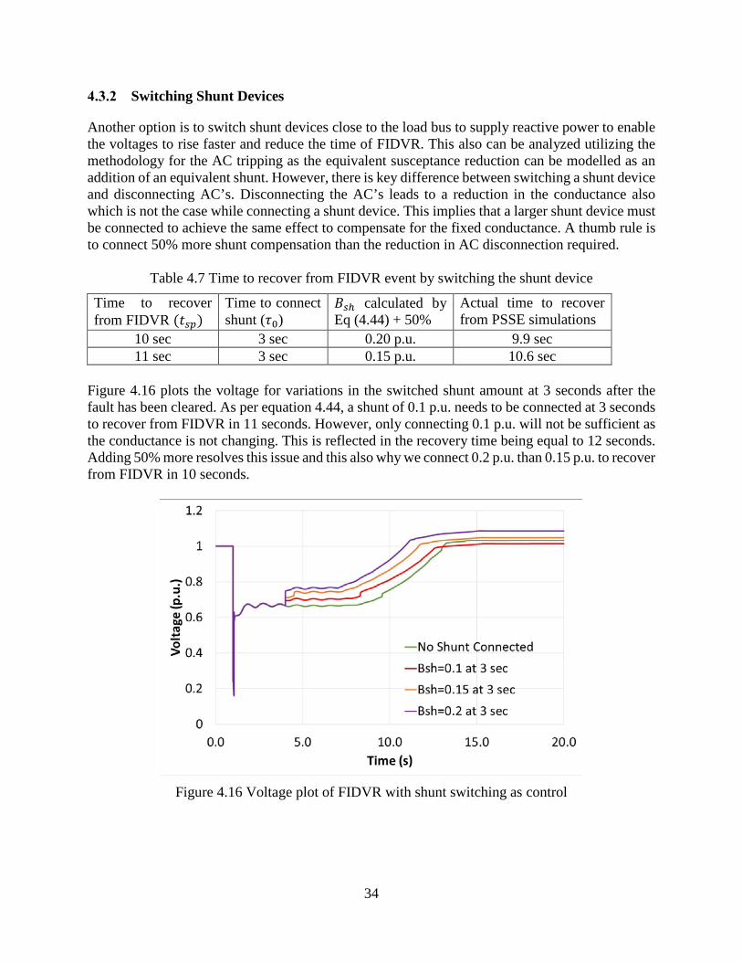
34

Switching Shunt Devices

Another option is to switch shunt devices close to the load bus to supply reactive power to enable the voltages to rise faster and reduce the time of FIDVR. This also can be analyzed utilizing the methodology for the AC tripping as the equivalent susceptance reduction can be modelled as an addition of an equivalent shunt. However, there is key difference between switching a shunt device and disconnecting AC’s. Disconnecting the AC’s leads to a reduction in the conductance also which is not the case while connecting a shunt device. This implies that a larger shunt device must be connected to achieve the same effect to compensate for the fixed conductance. A thumb rule is to connect 50% more shunt compensation than the reduction in AC disconnection required.

Table 4.7 Time to recover from FIDVR event by switching the shunt device

Time to recover from FIDVR (𝑉𝑉𝑠𝑠𝑠𝑠)

Time to connect shunt (𝜏𝜏0)

𝐵𝐵𝑠𝑠ℎ calculated by Eq (4.44) + 50%

Actual time to recover from PSSE simulations

10 sec 3 sec 0.20 p.u. 9.9 sec 11 sec 3 sec 0.15 p.u. 10.6 sec

Figure 4.16 plots the voltage for variations in the switched shunt amount at 3 seconds after the fault has been cleared. As per equation 4.44, a shunt of 0.1 p.u. needs to be connected at 3 seconds to recover from FIDVR in 11 seconds. However, only connecting 0.1 p.u. will not be sufficient as the conductance is not changing. This is reflected in the recovery time being equal to 12 seconds. Adding 50% more resolves this issue and this also why we connect 0.2 p.u. than 0.15 p.u. to recover from FIDVR in 10 seconds.

Figure 4.16 Voltage plot of FIDVR with shunt switching as control

35

5. Real Time Test Bed Implementation of Algorithms in OpenPDC

An important deliverable in this project is the implementation of the methodologies in a real time test bed and an evaluation of their applicability in real-time operations. As we are dealing with phasor data, we need to use a Phasor Data Concentrator (PDC) to implement our techniques to run in real-time. For this project, we use the OpenPDC, an open-source PDC as it is open-source and is used by utilities to analyze data from PMU’s in the field. We have implemented the following real-time phasor analytics in OpenPDC

1. W-Index Calculation for quantifying FIDVR for Voltage waveform (CSV output along with Visualization)

2. Lyapunov Exponent to determine the short-term voltage stability (CSV output along with Visualization)

These methods have been compiled into dll files that the utilities can directly use in their OpenPDC instance. The output of the method is either a CSV output file for analyzing any data after the event has happened or it can be visualized as a plot in real-time giving the operators at the utilities a real-time indication of the system stability. Figures 8 & 9 plot the W-Index and the Lyapunov Exponent for two voltage waveforms (on the top) that demonstrate short term voltage stability and FIDVR respectively.

Figure 5.1 Delayed voltage response (top) and the corresponding W-index (bottom) vs the time in samples (60

samples per sec).

Figure 5.2 Voltage instability event (top)

and the corresponding Lyapunov Exponent (bottom) vs the time in sample (60 samples

per sec).

The W-index stays near 0 and even goes positive around 3 seconds after the event. This low value will enable us to conclude a severe FIDVR event and initiate mitigation schemes. The Lyapunov

36

Exponent goes positive very quickly after the event, implying a severe voltage stability problem and enables us to initiate mitigation schemes. The C# code for calculating the W-index in OpenPDC is present in Appendix 2 with various comments enabling readers to implement the methodology. At present, it outputs the data as an output adapter into a csv file that is prespecified by the user for a set of voltages.

37

6. Conclusion

In this project, the problem of monitoring and mitigating FIDVR is addressed by utilizing the high sampling rate of PMU’s and understanding the physics underlying the FIDVR problem to issue control signals to smart thermostats and shunt devices in real-time. The initial methodology to understand and monitor is based on the voltage measurements being made at the transmission substation where the FIDVR is manifested. To ensure the robustness of the proposed methodology, the voltage waveform measured at the PMU is converted into a time varying probability distributions that is compared to another time varying probability distributions derived from a predefined voltage waveform that is determined by the reliability coordinator. The comparison between the probability distributions is performed using the Wasserstein metric that has the appealing properties of continuity and a limited output. This ensures that the measure calculated at the PMU is robust and reliable. The methods are implemented for real-time validation in OpenPDC to verify that they can indeed operate in the real-time environment and that they can handle noise introduced by measurement error and delays in the communication network. OpenPDC is chosen as it is in use by the utilities and so the code developed can be directly ported into the utilities’ operations with minimal effort. To determine the control, just utilizing the voltage did not provide sufficient information as several varying parameters of the load can lead to similar voltages. To overcome this, the composite load model is studied in detail and is simplified based on engineering judgment and it is shown that an admittance approach is well suited for this purpose. Analytical relations were derived by approximations of expressions and the time to recovery in terms of the measured admittance is derived. This is verified on PSSE simulations and the error between the expected times and the measured times to recovery were less than 1 second. The low error provides confidence on utilizing this method for control to ensure that the FIDVR recovery can occur within a pre-specified time. The only control schemes that can mitigate FIDVR are shown to be the tripping of Air Conditioners or the injection of reactive power via Shunt devices. An analytical expression for the magnitude of control action as a function of trip time is derived and this is also tested in PSSE. The expression is shown to be accurate to within 1 second with control actions upto 30% Air conditioner load tripping and provides a use case for the utilities to implement smart thermostats in their distribution network.

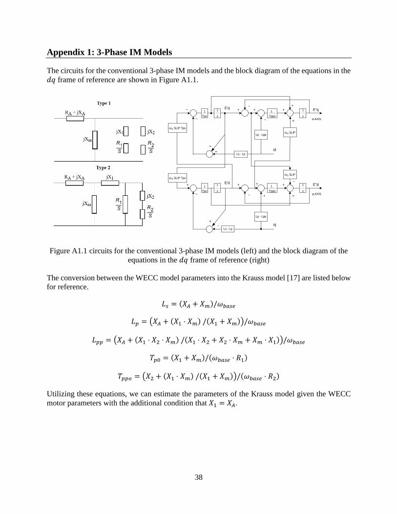
38

Appendix 1: 3-Phase IM Models

The circuits for the conventional 3-phase IM models and the block diagram of the equations in the 𝑖𝑖𝑑𝑑 frame of reference are shown in Figure A1.1.

Lp - Lpp

d-AXIS

id

E'q

Ls - Lp

E"q1Tppo s

1

s

11Tpo

ωo SLIPωo SLIP Tpo

Lp - Lpp

q-AXIS

iq

E'd

Ls - Lp

E"d1Tppo s

1

s

11Tpo

ωo SLIPωo SLIP Tpo

Figure A1.1 circuits for the conventional 3-phase IM models (left) and the block diagram of the

equations in the 𝑖𝑖𝑑𝑑 frame of reference (right) The conversion between the WECC model parameters into the Krauss model [17] are listed below for reference.

𝐾𝐾𝑠𝑠 = (𝑋𝑋𝑚𝑚 + 𝑋𝑋𝑚𝑚)/𝜔𝜔𝑏𝑏𝑠𝑠𝑠𝑠𝑒𝑒

𝐾𝐾𝑠𝑠 = �𝑋𝑋𝑚𝑚 + (𝑋𝑋1 ⋅ 𝑋𝑋𝑚𝑚) /(𝑋𝑋1 + 𝑋𝑋𝑚𝑚)�/𝜔𝜔𝑏𝑏𝑠𝑠𝑠𝑠𝑒𝑒

𝐾𝐾𝑠𝑠𝑠𝑠 = �𝑋𝑋𝑚𝑚 + (𝑋𝑋1 ⋅ 𝑋𝑋2 ⋅ 𝑋𝑋𝑚𝑚) /(𝑋𝑋1 ⋅ 𝑋𝑋2 + 𝑋𝑋2 ⋅ 𝑋𝑋𝑚𝑚 + 𝑋𝑋𝑚𝑚 ⋅ 𝑋𝑋1)�/𝜔𝜔𝑏𝑏𝑠𝑠𝑠𝑠𝑒𝑒

𝑇𝑇𝑠𝑠0 = (𝑋𝑋1 + 𝑋𝑋𝑚𝑚)/(𝜔𝜔𝑏𝑏𝑠𝑠𝑠𝑠𝑒𝑒 ⋅ 𝑅𝑅1)

𝑇𝑇𝑠𝑠𝑠𝑠𝑡𝑡 = �𝑋𝑋2 + (𝑋𝑋1 ⋅ 𝑋𝑋𝑚𝑚) /(𝑋𝑋1 + 𝑋𝑋𝑚𝑚)�/(𝜔𝜔𝑏𝑏𝑠𝑠𝑠𝑠𝑒𝑒 ⋅ 𝑅𝑅2)

Utilizing these equations, we can estimate the parameters of the Krauss model given the WECC motor parameters with the additional condition that 𝑋𝑋1 = 𝑋𝑋𝑚𝑚.

39

Appendix 2: C# Code implementing KL-index & W-Index in OpenPDC

//For more information contact Amar (amar@iastate.edu) using GSF; using GSF.TimeSeries; using GSF.TimeSeries.Adapters; using System; using System.Collections.Generic; using System.ComponentModel; using System.Diagnostics; using System.IO; using System.Linq; using System.Text; using System.Threading.Tasks; namespace KLWOutputAdapater { [Description("KLWOutputAdapater : Writes KLW average into a CSV file")] public class KLWAdapter : OutputAdapterBase { #region [ Members ] //Fields - Part of OutputAdapterBase private string m_fileName; // The file name to write into private StreamWriter m_outStream; // Output File name private int m_measurementCount; // Measurement Count //Useful for custom implementation // To write header into the CSV File private bool header_written = false; // Threshold Value to trigger action private double ThresholdTriggerValue; // Parameters to be passed as values for the custom action private double ChangingParameter1, ChangingParameter2; //A set of dictionaries to keep track of the measurements //Key : Measurement ID , Value : A queue of measurement values private Dictionary<Guid, Queue<double>> measurement_dictionary; //Key : Measurement ID , Value : Dictionary of <Value of Voltage bin , Histogram count> pairs private Dictionary<Guid, SortedDictionary<double, int>> measurement_Histogram_dictionary; //Key : Measurement ID , Value : Dictionary of <Value of Voltage bin , Histogram count> pairs private Dictionary<Guid, SortedDictionary<double, int>> KL_W_Reference_Histogram_dictionary; //Key : Measurement ID , Value : KLW iteration count private Dictionary<Guid, int> KL_W_iteration_dictionary;

40

//Key : Measurement ID , Value : start flag private Dictionary<Guid, bool> KL_W_start_flag_dictionary; //Key : Measurement ID , Value : window over flag private Dictionary<Guid, bool> KL_W_window_over_flag_dictionary; //Key : Measurement ID , Value : KLW values private Dictionary<Guid, double> KL_W_dictionary; //Time between two measurement samples private double delta_time; //Initial reference voltage private double V1; //rise time private double Tc; //should be 180 for KL and 45 for LE private int window_length; //Percentage trigger private double percentage_trigger; // First Measurement Key private MeasurementKey FirstMeasurementKey; //Value of first window average private double first_average; #endregion #region [ Overridden Methods ] /// <summary> /// Gets or sets the name of the CSV file. /// </summary> [ConnectionStringParameter, Description("Define the name of the CSV file to which measurements will be archived."), DefaultValue("measurements_test.csv"), CustomConfigurationEditor("GSF.TimeSeries.UI.WPF.dll", "GSF.TimeSeries.UI.Editors.FileDialogEditor", "type=save; defaultExt=.csv; filter=CSV files|*.csv|All files|*.*")] public string FileName { get { return m_fileName; } set { m_fileName = value; } }

41

/// <summary> /// Returns a flag that determines if measurements sent to this /// <see cref="CustomCSVOutputAdapter"/> are destined for archival. /// </summary> public override bool OutputIsForArchive { get { return true; } } /// <summary> /// Gets a flag that determines if this <see cref="CustomCSVOutputAdapter"/> /// uses an asynchronous connection. /// </summary> protected override bool UseAsyncConnect { get { return false; } } /// <summary> /// Gets a short one-line status of this <see cref="CSVOutputAdapter"/>. /// </summary> /// <param name="maxLength">Maximum length of the status message.</param> /// <returns>Text of the status message.</returns> public override string GetShortStatus(int maxLength) { return string.Format("Archived {0} measurements to File : {1} in the custom format", m_measurementCount, m_fileName).CenterText(maxLength); } /// <summary> /// Attempts to connect to this <see cref="CustomCSVOutputAdapter"/>. /// </summary> protected override void AttemptConnection() { m_outStream = new StreamWriter(m_fileName); } // <summary> /// Attempts to disconnect from this <see cref="CustomCSVOutputAdapter"/>. /// </summary> protected override void AttemptDisconnection() { m_outStream.Close(); }

42

/// <summary> /// Initializes this <see cref="CustomCSVOutputAdapter"/>. /// </summary> public override void Initialize() { base.Initialize(); Dictionary<string, string> settings = Settings; string setting; string Temporary; // Load optional parameters if (settings.TryGetValue("FileName", out setting)) m_fileName = setting; if (settings.TryGetValue("TriggerValue", out Temporary)) //If the TriggerValue is not given b the user, it is null and will throw an exception when converitng to double. ThresholdTriggerValue = (Temporary.Equals("") || Temporary == null) ? 0 : Convert.ToDouble(Temporary); if (settings.TryGetValue("ChangingParameter1Value", out Temporary)) //If the TriggerValue is not given b the user, it is null and will throw an exception when converitng to double. ChangingParameter1 = (Temporary.Equals("") || Temporary == null) ? 0 : Convert.ToDouble(Temporary); if (settings.TryGetValue("ChangingParameter2Value", out Temporary)) //If the TriggerValue is not given b the user, it is null and will throw an exception when converitng to double. ChangingParameter2 = (Temporary.Equals("") || Temporary == null) ? 0 : Convert.ToDouble(Temporary); if (settings.TryGetValue("DeltaTime", out Temporary)) //If the Delta Time is not given by the user, it is zero and will throw a divide by zero exception delta_time = (Temporary.Equals("") || Temporary == null) ? 1.0/60 : Convert.ToDouble(Temporary); if (settings.TryGetValue("InitialReferenceVoltage", out Temporary)) //If the Initial Reference Voltage is not given by the user, it is zero and will throw a divide by zero exception V1 = (Temporary.Equals("") || Temporary == null) ? 0.55 : Convert.ToDouble(Temporary); if (settings.TryGetValue("RiseTime", out Temporary)) //If the rise time is not given by the user, it is zero and will throw a divide by zero exception Tc = (Temporary.Equals("") || Temporary == null) ? 5.0 : Convert.ToDouble(Temporary); if (settings.TryGetValue("WindowLength", out Temporary)) //If the window length is not given by the user, it is zero and will throw a divide by zero exception window_length = (Temporary.Equals("") || Temporary == null) ? 0 : Convert.ToInt32(Temporary); //SetPythonProcessInfo();

43

/* Inputs from User : FileName=E:\testing_csv_trial43b.csv; InputMeasurementKeys=069c5e29-f78a-46f6-9dff-c92cb4f69371; RequeueOnException=False; TriggerValue=400000; ChangingParameter1Value=100; ChangingParameter2Value=200; InitialReferenceVoltage = 0.55; RiseTime = 5.0; window_length = 180; percentage_trigger = 0.02 */ //Intializing the dictionaries measurement_dictionary = new Dictionary<Guid, Queue<double>>(2 * window_length); measurement_Histogram_dictionary = new Dictionary<Guid, SortedDictionary<double, int>>(); KL_W_Reference_Histogram_dictionary = new Dictionary<Guid, SortedDictionary<double, int>>(); KL_W_iteration_dictionary = new Dictionary<Guid, int>(2 * window_length); KL_W_start_flag_dictionary = new Dictionary<Guid, bool>(); KL_W_window_over_flag_dictionary = new Dictionary<Guid, bool>(); KL_W_dictionary = new Dictionary<Guid, double>(); } // <summary> /// Used to process the measurements that come in. /// <param name="measurements">List of Measurements at this moment</param> /// </summary> protected override void ProcessMeasurements(IMeasurement[] measurements) { if ((object)measurements != null) { StringBuilder builder = new StringBuilder(); StringBuilder manipulated_builder = new StringBuilder(); if (!header_written) builder.Append(WriteHeader(measurements)); FirstMeasurementKey = measurements[0].Key; // Get the first measurement key int number_of_measurement_keys = measurements.MeasurementKeys().Length; for (int i = 0; i < measurements.Length; i = i + number_of_measurement_keys) { builder.Append((long)measurements[i].Timestamp); for (int j = 0; j < measurements.Select(m => m.Key).Distinct().ToArray().Length; j++) { builder.Append(',').Append(measurements[i + j].AdjustedValue);

44

//Append the output of the moving average string KL_W_value = Calculate_KL_W_InMeasurement(measurements[i + j].ID, window_length, delta_time); manipulated_builder.Append(KL_W_value); } builder.Append(manipulated_builder.ToString()); // append the string received from the calculate average method builder.Append(Environment.NewLine); } m_outStream.Write(builder.ToString()); // Write to the stream m_measurementCount += measurements.Length; } } #endregion #region [ Custom Methods] /// <summary> /// Calculate the first average of the current measurement /// </summary> /// <param name="dictionary">Dictionary of Timestamp and values</param> public void CalculateFirstAverage(Dictionary<long, double> dictionary) { first_average = dictionary.Take(window_length).ToDictionary(pair => pair.Key, pair => pair.Value).Values.Average(); } /// <summary> /// Initialize Histogram /// </summary> /// <param name="NBins">Number of bins in the histogram</param> /// <returns></returns> public SortedDictionary<double, int> InitializeHistogram(int NBins) { double range = 1.05 * first_average; SortedDictionary<double, int> HistogramDictionary = new SortedDictionary<double, int>(); double increment = range / NBins; double start = 0; while (start <= range) { HistogramDictionary.Add(start, 0); // Amar - Can we do this once instead of every time?? start += increment; } return HistogramDictionary; } /// <summary> /// Add the /// </summary> /// <param name="measurement_id">current measurment ID</param> /// <param name="value">value</param>

45

/// <param name="type">reference/measurement</param> /// <returns></returns> public SortedDictionary<double, int> AddToHistogram(Guid measurement_id, double value, string type) { SortedDictionary<double, int> HistogramDictionary = new SortedDictionary<double, int>(); if (type == "reference") { HistogramDictionary = KL_W_Reference_Histogram_dictionary[measurement_id]; } else if (type == "measurement") { HistogramDictionary = measurement_Histogram_dictionary[measurement_id]; } /*else { int x;// For testing }*/ double valueRange = HistogramDictionary.Keys.Where(key => value >= key).Last(); HistogramDictionary[valueRange]++; return HistogramDictionary; } public SortedDictionary<double, int> RemoveFromHistogram(Guid measurement_id, double value, string type) { SortedDictionary<double, int> HistogramDictionary = new SortedDictionary<double, int>(); if (type == "reference") { HistogramDictionary = KL_W_Reference_Histogram_dictionary[measurement_id]; } else if (type == "measurement") { HistogramDictionary = measurement_Histogram_dictionary[measurement_id]; } else { int x;// For testing } double valueRange = HistogramDictionary.Keys.Where(key => value >= key).Last(); HistogramDictionary[valueRange]--; return HistogramDictionary; } public double SumAbsCum(SortedDictionary<double, int> dictionary) { double sum = 0, sum2 = 0, sum3 = 0, n = 0;

46

foreach (double key in dictionary.Keys) { sum += dictionary[key]; // getting the cumulative sum sum2 += Math.Abs(sum); // sum of abs cumulative sums sum3 += n * dictionary[key];//difference of the means of the 2 distributions n++; } return 2 * sum2 * sum3 / Math.Sqrt(dictionary.Keys.Count) / n;// divide by is to normalise the sum3 } public SortedDictionary<double, int> SubtractDictionary(SortedDictionary<double, int> first, SortedDictionary<double, int> second) { SortedDictionary<double, int> SubtractedDictionary = new SortedDictionary<double, int>(); if (first.Count == second.Count) { foreach (double key in first.Keys) SubtractedDictionary.Add(key, first[key] - second[key]); } return SubtractedDictionary; } public string Calculate_KL_W_InMeasurement(Guid measurement_id, int window_length, double delta_time) { StringBuilder builder = new StringBuilder(); Queue<double> measurement_queue; SortedDictionary<double, int> measurement_Histogram; SortedDictionary<double, int> KL_W_Reference_Histogram; double Appending_term_reference; double KL_W_value; int KL_W_iteration_value = 0; bool KL_W_start_flag_value = false; bool KL_W_window_over_flag_value = false; if (!measurement_dictionary.TryGetValue(measurement_id, out measurement_queue)) { measurement_queue = new Queue<double>(); measurement_dictionary.Add(measurement_id, measurement_queue); } if (!measurement_Histogram_dictionary.TryGetValue(measurement_id, out measurement_Histogram)) { measurement_Histogram = new SortedDictionary<double, int>(); measurement_Histogram_dictionary.Add(measurement_id, measurement_Histogram); } if (!KL_W_Reference_Histogram_dictionary.TryGetValue(measurement_id, out KL_W_Reference_Histogram)) { KL_W_Reference_Histogram = new SortedDictionary<double, int>();

47

KL_W_Reference_Histogram_dictionary.Add(measurement_id, KL_W_Reference_Histogram); } if (!KL_W_dictionary.TryGetValue(measurement_id, out KL_W_value)) { KL_W_dictionary.Add(measurement_id, KL_W_value); } if (!KL_W_iteration_dictionary.TryGetValue(measurement_id, out KL_W_iteration_value)) { KL_W_iteration_dictionary.Add(measurement_id, KL_W_iteration_value); } if (!KL_W_start_flag_dictionary.TryGetValue(measurement_id, out KL_W_start_flag_value)) { KL_W_start_flag_dictionary.Add(measurement_id, KL_W_start_flag_value); } if (!KL_W_window_over_flag_dictionary.TryGetValue(measurement_id, out KL_W_window_over_flag_value)) { KL_W_window_over_flag_dictionary.Add(measurement_id, KL_W_window_over_flag_value); } if (measurement_queue.Count == window_length) { //measurement_log_voltage_diff_queue.Enqueue((Math.Log(Math.Abs(measurement_queue.Peek()-measurement_queue.ElementAt(2))/10000+0.001))); double a = measurement_queue.ElementAt(window_length - 1); double b = measurement_queue.ElementAt(window_length - 2); if (a < 60000) { int x = 0; } if (KL_W_start_flag_dictionary[measurement_id] == false) { if (((measurement_queue.ElementAt(window_length - 1) - measurement_queue.ElementAt(window_length - 2)) > first_average * percentage_trigger)) //if( (a-b)) { KL_W_start_flag_dictionary[measurement_id] = true; KL_W_Reference_Histogram_dictionary[measurement_id] = InitializeHistogram(108); //InitializeHistogram(measurement_id, 108); measurement_Histogram_dictionary[measurement_id] = InitializeHistogram(108); //InitializeHistogram(measurement_id, 108); } else { KL_W_start_flag_dictionary[measurement_id] = false; } } else // this implies KL_W_start_flag_dictionary[measurement_id] = true; { KL_W_start_flag_dictionary[measurement_id] = true; }

48

if (measurement_queue.Count == window_length && KL_W_start_flag_dictionary[measurement_id] == true) { if (KL_W_window_over_flag_dictionary[measurement_id] == false) { if (((measurement_queue.ElementAt(1) - measurement_queue.ElementAt(0)) > first_average * percentage_trigger)) { KL_W_window_over_flag_dictionary[measurement_id] = true; } else { KL_W_window_over_flag_dictionary[measurement_id] = false; } } else // automatically implies KL_W_window_over_flag_dictionary[measurement_id] = true; { KL_W_window_over_flag_dictionary[measurement_id] = true; } if ((KL_W_Reference_Histogram.Values.ToArray().Sum()) < window_length - 2) { //builder.Append(","); //builder.Append("KL Window - Small"); Appending_term_reference = first_average * (V1 + (1 - V1) * (1 - Math.Exp(-delta_time * KL_W_iteration_dictionary[measurement_id] / Tc))); // this 0.45 & 3 can be changed KL_W_Reference_Histogram_dictionary[measurement_id] = AddToHistogram(measurement_id, Appending_term_reference, "reference"); measurement_Histogram_dictionary[measurement_id] = AddToHistogram(measurement_id, measurement_queue.ElementAt(window_length - 1), "measurement"); KL_W_dictionary[measurement_id] = SumAbsCum(SubtractDictionary(KL_W_Reference_Histogram_dictionary[measurement_id], measurement_Histogram_dictionary[measurement_id])); //builder.Append(","); builder.Append(KL_W_dictionary[measurement_id] / (1 + KL_W_iteration_dictionary[measurement_id]) / (1 + KL_W_iteration_dictionary[measurement_id])); KL_W_iteration_dictionary[measurement_id]++; } else if ((KL_W_Reference_Histogram.Values.ToArray().Sum()) >= window_length - 2) // should coincide with KL_W_window_over_flag_dictionary[measurement_id] = true; { if (KL_W_window_over_flag_dictionary[measurement_id] == true) { Appending_term_reference = first_average * (V1 + (1 - V1) * (1 - Math.Exp(-delta_time * KL_W_iteration_dictionary[measurement_id] / Tc))); // this 0.45 & 3 can be changed KL_W_Reference_Histogram_dictionary[measurement_id] = AddToHistogram(measurement_id, Appending_term_reference, "reference"); measurement_Histogram_dictionary[measurement_id] = AddToHistogram(measurement_id, measurement_queue.ElementAt(window_length - 1), "measurement");

49

KL_W_dictionary[measurement_id] = SumAbsCum(SubtractDictionary(KL_W_Reference_Histogram_dictionary[measurement_id], measurement_Histogram_dictionary[measurement_id])); //builder.Append(","); builder.Append(KL_W_dictionary[measurement_id] / (1 + KL_W_iteration_dictionary[measurement_id]) / (1 + KL_W_iteration_dictionary[measurement_id])); //Removing_term_reference = first_average * (V1 + (1 - V1) * (1 - Math.Exp(-delta_time * (KL_W_iteration_dictionary[measurement_id] - (window_length - 2))/Tc))); // this 0.45 & 3 can be changed //KL_W_Reference_Histogram_dictionary[measurement_id] = RemoveFromHistogram(measurement_id, Removing_term_reference, "reference"); //measurement_Histogram_dictionary[measurement_id] = RemoveFromHistogram(measurement_id, measurement_queue.Peek(), "measurement"); KL_W_iteration_dictionary[measurement_id]++; } else// should not come here { builder.Append(","); builder.Append("Check indices"); } } } } if (KL_W_iteration_dictionary[measurement_id] > 2000) { //measurement_log_voltage_diff_queue.Clear(); KL_W_start_flag_dictionary[measurement_id] = false; KL_W_window_over_flag_dictionary[measurement_id] = false; KL_W_iteration_dictionary[measurement_id] = 0; KL_W_dictionary[measurement_id] = 0; KL_W_Reference_Histogram_dictionary[measurement_id].Clear(); measurement_Histogram_dictionary[measurement_id].Clear(); //measurement_LE_initial_dictionary[measurement_id] = 0; } return builder.ToString(); } /// <summary> /// /// </summary> /// <param name="measurements"></param> /// <returns></returns> private string WriteHeader(IMeasurement[] measurements) { StringBuilder builder = new StringBuilder(); builder.Append("Timestamp"); MeasurementKey[] unique_measurement_keys = measurements.Select(m => m.Key).Distinct().ToArray(); foreach (MeasurementKey key in unique_measurement_keys) builder.Append(",").Append(key); //To be included- foreach (MeasurementKey key in unique_measurement_keys)

50

builder.Append(",").Append(key).Append("-").Append("Moving Average").Append(",").Append(key).Append("-").Append("LE Calculated"); builder.Append(Environment.NewLine); header_written = true; return builder.ToString(); } #endregion } }

51

References

[1] P. Kundur, J. Paserba, V. Ajjarapu, G. Andersson, A. Bose, C. Canizares, N. Hatziar-gyriou, D. Hill, A. Stankovic, C. Taylor, T. Van Cutsem, and V. Vittal, “Definition and classification of power system stability IEEE/CIGRE joint task force on stability terms and definitions,” Power Systems, IEEE Transactions on, vol. 19, no. 3, pp. 1387–1401, 2004.

[2] M. Paramasivam, A. Salloum, V. Ajjarapu, V. Vittal, N. B. Bhatt and S. Liu, "Dynamic Optimization Based Reactive Power Planning to Mitigate Slow Voltage Recovery and Short Term Voltage Instability," in IEEE Transactions on Power Systems, vol. 28, no. 4, pp. 3865-3873, Nov. 2013.

[3] M. Paramasivam,” Dynamic optimization based reactive power planning for improving short-term voltage performance”, PhD Dissertation, Iowa State University.

[4] M. Paramasivam, S. Dasgupta, V. Ajjarapu and U. Vaidya, "Contingency Analysis and Identification of Dynamic Voltage Control Areas," in IEEE Transactions on Power Systems, vol. 30, no. 6, pp. 2974-2983, Nov. 2015.

[5] S. Sinha, P. Sharma, U. Vaidya and V. Ajjarapu, “Identifying Causal Interaction in Power System: Information-Based Approach”, accepted for publication in Conference in Decision and Control, 2017.

[6] Modeling and validation work group, “White paper on modeling and studying FIDVR events,” Western Electricity Coordinating Council, Technical Report, October 20, 2011.

[7] North American Electric Reliability Corporation, Reliability Standard TPL-001-4, Transmission System Planning Performance Requirements.

[8] North American Transmission Forum, Transient voltage criteria reference document, September 2016.

[9] Modeling and validation work group, “WECC Dynamic Composite Load Model Specifications,” Western Electricity Coordinating Council, Technical Report, January 25, 2015.

[10] Paul Krauss, “Analysis of Electric Machinery and Drive Systems”, 2nd Edition. [11] S. Dasgupta, M. Paramasivam, U. Vaidya and V. Ajjarapu, "Real-Time Monitoring of Short-

Term Voltage Stability Using PMU Data," in IEEE Transactions on Power Systems, vol. 28, no. 4, pp. 3702-3711, Nov. 2013.

[12] A. Reddy and V. Ajjarapu, "PMU based real-time monitoring for delayed voltage response," 2015 North American Power Symposium (NAPS), Charlotte, NC, 2015, pp. 1-6.

[13] S. Dasgupta, M. Paramasivam, U. Vaidya and V. Ajjarapu, "Entropy-Based Metric for Characterization of Delayed Voltage Recovery," in IEEE Transactions on Power Systems, vol. 30, no. 5, pp. 2460-2468, Sept. 2015.

[14] Olkin, I. and Pukelsheim, F. (1982). "The distance between two random vectors with given dispersion matrices". Linear Algebra Appl. 48: 257–263.

[15] S. Halpin, K. Harley, R. Jones, and L. Taylor, “Slope-permissive under-voltage load shed relay for delayed voltage recovery mitigation,” Power Systems, IEEE Transactions on, vol. 23, no. 3, pp. 1211 –1216, Aug. 2008

[16] A. Radaideh, U. Vaidya and V. Ajjarapu, "Sequential Set-point Control for Heterogeneous Thermostatically Controlled Loads Through an Extended Markov Chain Abstraction," in IEEE Transactions on Smart Grid, vol. PP, no. 99, pp. 1-1.

[17] Siemens PTI Power Technologies Inc., PSS/E 33, Program Application Guide, Vol. II, May 2011

Part II

Real Time Synchrophasor Measurements

Based Long Term Voltage Stability Monitoring and Control

Chen-Ching Liu

Ruoxi Zhu, Graduate Student

Washington State University

For information about Part II, contact Dr. Chen-Ching Liu School of Electrical Engineering and Computer Science Washington State University Pullman, WA, 99164-2752 Email: liu@wsu.edu Phone: 509-335-1150 Power Systems Engineering Research Center The Power Systems Engineering Research Center (PSERC) is a multi-university Center conducting research on challenges facing the electric power industry and educating the next generation of power engineers. More information about PSERC can be found at the Center’s website: http://www.pserc.org. For additional information, contact: Power Systems Engineering Research Center Arizona State University Engineering Research Center #527 551 E. Tyler Mall Tempe, Arizona 85287-5706 Phone: 480-965-1643 Fax: 480-727-2052 Notice Concerning Copyright Material PSERC members are given permission to copy without fee all or part of this publication for internal use if appropriate attribution is given to this document as the source material. This report is available for downloading from the PSERC website.

2017 Washington State University. All rights reserved.

i

Table of Contents

1. Introduction ..................................................................................................................................1

1.1 Background ...........................................................................................................................1

1.2 Overview of the problem .......................................................................................................1

1.3 Report organization ...............................................................................................................2

2. Voltage Stability Assessment Index ............................................................................................3

2.1 Formulation of VSAI ............................................................................................................3

2.2 Simulation for VSAI-I ...........................................................................................................3

2.3 VSAI with voltage dynamic mechanisms (VSAI-II) ............................................................5

2.4 Simulation results: VSAI-I and VSAI-II ...............................................................................6

2.5 Summary ...............................................................................................................................7

3. OPF-LI .........................................................................................................................................9

3.1 Formulation of OPF-LI .........................................................................................................9

3.1.1 Ward-PV model .............................................................................................................9

3.1.2 OPF based algorithm ...................................................................................................10

3.2 Simulation results for OPF-LI .............................................................................................10

3.2.1 Constructing the Ward- PV equivalent ........................................................................12

3.2.2 Estimate the voltage stability margin ..........................................................................12

3.2.3 TSAT validation ..........................................................................................................12

3.3 Summary .............................................................................................................................14

4. OPF-LI with state calculator ......................................................................................................15

4.1 PMU measurement-based state calculator ..........................................................................15

4.2 OPF-LI with SC ..................................................................................................................15

4.3.1 Simulation results: Case 1 ...........................................................................................16

4.3.2 Simulation results of Case 2 ........................................................................................18

4.4 Summary .............................................................................................................................19

5. OPF-LI with OLTC control .......................................................................................................20

5.1 OLTC dynamic mechanism ................................................................................................20

5.1.1 OLTC model ................................................................................................................20

5.1.2 OLTC dynamic mechanism for a simple system ........................................................21

5.1.3 OLTC dynamic mechanism for power system with M OLTCs ..................................22

5.2 OLTC operating control ......................................................................................................23

ii

5.3 OPF-LI with OLTC control .................................................................................................24

5.4 Simulation results ................................................................................................................25

5.5 Summary .............................................................................................................................27

6. Conclusions ................................................................................................................................28

References ......................................................................................................................................29

iii

List of Figures

Figure 2.1 VSAI and voltage magnitudes for IEEE-30 bus system at the base case ...................... 4

Figure 2.2 VSAI and voltage magnitudes of IEEE 30-bus system after a contingency ................. 4

Figure 2.3 VSAI-I of the load buses ............................................................................................... 6

Figure 2.4 VSAI-II of the load buses .............................................................................................. 7

Figure 2.5 Thevenin equivalent model ........................................................................................... 7

Figure 3.1 Ward-PV model ............................................................................................................. 9

Figure 3.2 Area1 of WECC 179 bus system ................................................................................. 11

Figure 3.3 System states for loads in area1increased to1.25 or 1.26 ............................................ 13

Figure 4.1 State calculator results—Case1 ................................................................................... 17

Figure 4.2 Loading limit following the contigency--Case 1 ......................................................... 17

Figure 4.3 State calculator results—Case 2 .................................................................................. 18

Figure 4.4 Loading limit during the contigency--Case 2 .............................................................. 19

Figure 5.1 Equivalent circuit of a tap transformer ........................................................................ 20

Figure 5.2 A simple power system with an OLTC ....................................................................... 21

Figure 5.3 Dynamic mechanism for one OLTC system ............................................................... 22

Figure 5.4 OPF-LI with OLTC operating control ......................................................................... 24

Figure 5.5 Comparison of voltage profiles—without OLTC blocking control ............................ 25

Figure 5.6 Comparison of voltage profiles—with OLTC blocking control ................................. 26

iv

List of Tables

Table 3-1 Comparison of the equivalent system and the original system .................................... 12

Table 3-2 System state at loading limits ....................................................................................... 12

Table 3-3 Comparison of OPF-LI and TSAT ............................................................................... 13

Table 4-1 PMU placement ............................................................................................................ 16

Table 5-1 Comparison of voltage magnitude for blocked bus ...................................................... 26

Table 5-2 Comparison of base case load case and light load case ................................................ 27

1

1. Introduction

1.1 Background

As the scale and complexity of an interconnected power grid has increased significantly, major blackouts in power systems have occurred due to system instability. Long term voltage stability is a focus area for power system research. Since power systems can be operated close to the verge of voltage instability, it is necessary for dispatchers to monitor voltage stability in an on-line operating environment. A voltage collapse is characterized by the fact that the voltage magnitude of some buses declines over time. Many algorithms have been proposed to estimate the margin to voltage instability at an operation point. The mechanisms of voltage instability are reported in [1][2]. These papers introduce the nonlinear aspects of voltage dynamics. Based on the dynamic behavior, Thevenin equivalent based methods are developed. According to Thevenin equivalent, the voltage stability or reactive-power reserve indices can be obtained [3][4].The VIP method [3] is intended to use local measurements to track the Thevenin equivalent. In recent years there are also measurement-based methods to assess voltage stability from the available measurements [5][6]. The main objective of this work is to develop a methodology for long term voltage stability assessment using a reduced network given a limited number of phasor measurements.

1.2 Overview of the problem

Long term voltage stability refers to the stability problem that occurs over a relatively long time frame, such as several minutes. These stability problem usually involves slow acting devices such as thermostatically controlled loads, LTC transformers, and distribution voltage regulators. To assess the long term voltage stability for a power system, two classes of methods have been developed. One is a model based method. Base on the system topology and operation condition, several indices can be extracted from power flow equations. Using the Jacobian matrix, several modes can be derived from the eigenvalues. Once the critical mode becomes zero, the system is considered to be unstable [7]. For the detection of the unstable condition, continuous power flow method, bifurcation theory, and sensitivity methods are proposed [8],[9],[10]. The other class, which is also popular is the measurements based method. Since numerous measurements are installed on a power system, e.g., SCADA and PMU. It is critical to utilize these measurements, particularly the large amount of PMU data. Many methods are based on Thevenin Equivalent (TE), such as the methods proposed in [3], [11]. The computational simplicity makes Thevenin equivalent based approaches suitable for real time applications. Since Thevenin equivalent simplifies the system to a two-node system, the results obtained by comparing the equivalent impedance and load impedance may not be accurate, Researchers propose to extend the TE model to an n-node model [6].

2

This research addresses the critical issues by proposing two different methods. One is the Voltage Stability Assessment Index (VSAI) and the other is Optimal Power Flow-Loading Limit (OPF-LI). Both methods are intended for long-term voltage stability assessment. VSAI is a TE based method, which is used to calculate the indices in a non-iterative manner. Due to the shortcomings of TE model, OPF-LI is developed to assess the voltage stability margin for a load area. To utilize available PMU measurements, State Calculator (SC) is included in the algorithm to approximate the system states at the buses where PMU measurements are not available. The methods proposed in this research have been validated by test systems.

1.3 Report organization

The organization of the remaining chapters is as follows: Chapter 2 is a summary of the formulation of VSAI method. The improved approach, OPF-LI, for monitoring voltage stability of a load area is described in Chapter 3. In Chapter 4, OPF-LI with PMU measurements including estimates states calculated by SC is described. Then, OPF-LI incorporating OLTC operating control is discussed in Chapter 5. The conclusion of this report is provided in Chapter 6.

3

2. Voltage Stability Assessment Index

Long-term voltage stability involves slow acting equipment for which the time scale of the phenomena can be several minutes. The existing centralized model based approaches often use multiple power flows to compute the voltage stability margin of a system. Hence it is computationally burdensome and not suitable for real time applications. The VSAI algorithm is a hybrid approach using the PMU data and the network information to calculate voltage stability indices at a load bus. It computes the distance to the point of voltage collapse (PoC) in a non-iterative manner by making use of wide area phasor measurements and system topological information.

2.1 Formulation of VSAI

To calculate VSAI-I, the first version of VSAI, a linearized Jacobian matrix of the power system is obtained based on the topological data and the system parameters. Then, one derives one or more sets of additional system characteristics (e.g., estimated voltages and currents for all buses) based on the specified perturbations. Finally, the TE impedance is estimated based on the actual system parameters and the derived system parameters. An index called 'Voltage Stability Assessment Index (VSAI)' is computed at every load bus, i.e.,

(1)

where ‘k’ means the load bus k, the average value is the equivalent impedance, and /k kx w represents the load impedance based on the actual system parameters [3]. Note that the index is a value between 0 and 1, i.e., for any bus 'k', where k ϵ load bus. A VSAIk value near “0” indicates that the bus ‘k’ is highly stable while a VSAIk value near "1" indicates that the bus 'k' is on the verge of voltage instability. The original work of VSAI is reported in [12].

2.2 Simulation for VSAI-I

VSAI-I is a version of VSAI based on the steady state model of VSAI in Sec. 2.1. The performance of VSAI-I is validated by simulation with the IEEE 30-bus system test under different scenarios of deteriorating voltage stability conditions. Figure 2.1 shows the VSAI indices of all load buses in the system along with important system metrics for the base case. It can be observed that for the base case system with no contingency, the VSAI of all the load buses are low. The VSAI of the weakest bus in the system is that of Bus 19, for which 𝑉𝑉𝑉𝑉𝑉𝑉𝐼𝐼19 = 0.1251.

4

Figure 2.1 VSAI and voltage magnitudes for IEEE-30 bus system at the base case

In contrast, as shown in Figure 2.2, when the contingencies take place (i.e. when the transmission lines between Buses 6 & 8 and 6 & 28 are taken out of the system), the voltage magnitudes at the buses decreased, particularly at Bus 8. This is due to the fact that there is only one generator feeding Bus 8 after two lines are de-energized. This is indicated by a significantly increased VSAI (VSAI8=0.7159) of the affected load bus (Bus 8). Hence the system instability index is high.

Figure 2.2 VSAI and voltage magnitudes of IEEE 30-bus system after a contingency

0 5 10 15 20 25 300

0.2

0.4

0.6

0.8

1

Bus Number

Vm(in

p.u)

Voltage Magnitude of All Buses

0 5 10 15 20 25 300

0.1

0.2

0.3

0.4

0.5

0.6

0.7

0.8

Bus Number

VASI

0 5 10 15 20 25 300

0.2

0.4

0.6

0.8

1

Bus Number

Vm(in

p.u.)

Voltage Magnitude of All Buses

0 5 10 15 20 25 300

0.1

0.2

0.3

0.4

0.5

0.6

0.7

0.8

Bus Number

VASI

VSAI

5

This information is visualized at the control center giving the operator the critical locations for voltage stability, allowing the operator to take appropriate actions based on control actions suggested by the tool.

2.3 VSAI with voltage dynamic mechanisms (VSAI-II)

Here the second version of VSAI, VSAI-II, refers to the enhanced version of VSAI-I incorporating voltage dynamic mechanisms. The model improves the accuracy of the voltage stability index for the real-time environment. It is proposed in this study to incorporate the voltage dynamic mechanisms, including generator excitation capability, stator current limit, and on-load tap changers. The generator is modeled by a voltage source E behind a reactance Xd, where E varies in order to maintain the terminal voltage V at a constant V0 during a normal operating condition. The excitation voltage is limited, and the stator current I also has an upper limit Ilim. The main strategies are as follows.

1) Normal operation: V=V0, E< Elim , I< Ilim;

2) Operation at the excitation voltage limit: When 2 22 2 2

2 lim2 2

d d d

E VV E VP QX X X

+ + = ≥

, add a

virtual node n+1 at this PV bus, convert the original generator i to a PQ bus (P, Q are specified by the bus load) and the voltage magnitude of the new bus is specified as Elim. Update the admittance matrix and the power flow equations as follows:

New generator bus (PV bus): 2

1 1 ( 1) ( 1) ( 1) ( 1) 1 1( cos sin ) ( )n n i n i n i n i n i n nP E V G B E Gδ δ+ + + + + + + += + + (2) Original generator bus (PQ bus):

1

1( cos sin )

n

i i j ij ij ij ijj

P V V G Bδ δ+

=

= +∑

1

1( sin cos )

n

i i j ij ij ij ijj

Q V V G Bδ δ+

=

= −∑ (3)

where n+1 means that the number of buses increases considering the virtual bus, and the number of the virtual bus is n+1.

3) Operation at the stator current limit: When 2 2

2 2lim2

P Q I IV+

= ≥ , convert this PV bus to a constant

current generator. By doing so, the following equation can be used to modify power flow equation for this generator i.

2 2 2 2 2

2 2

2

1 1

*

( cos sin ) ( sin cos )

i i i i i

n n

i j ij ij ij ij j ij ij ij ijj j

S V I P Q

V V G B V G Bδ δ δ δ= =

= = +

= + + − ∑ ∑

(4)

6

On-Load Tap Changers (OLTCs) are used to maintain constant load voltages. An OLTC has a reference voltage value V0, which is the target value of automatic control. The tap movements are discrete and modeled by:

1 0( )k k kn n d f V V+ = − ⋅ − 1 ,

( ) 0 ,1 ,

if x vf x if x v

if x v

− < −∆= < ∆ > ∆

(5)

Then update the tap-ratio of this load bus and, at the same time, the admittance matrix should be modified. Incorporating the voltage dynamic mechanism, the results of the state variables would be modified, hence the method is more accurate in representing the voltage behaviors in the real-time environment.

2.4 Simulation results: VSAI-I and VSAI-II

The WECC 179 bus system is used as the test system for comparison of the results obtained from VSAI-I and VSAI-II. Contingency: Increase load in Area1 to 1.1 times of base case loading

Figure 2.3 VSAI-I of the load buses

0 20 40 60 80 100 120 140 160 180

Bus number(WECC179)

0

0.2

0.4

0.6

0.8

1

VSAI

-I

X: 165

Y: 0.8978X: 71

Y: 0.8049

7

Figure 2.4 VSAI-II of the load buses

As shown in Figure 2.3, some values of the VSAI-I are equal to 1, indicating the system is close to instability. However, for VSAI-II, most values are equal to 1 indicating that the stability margin is small. For both cases, the results show the system is on the verge of voltage instability. Since no dynamic mechanism is modeled in the VSAI-I index, the system condition reflected by the upper diagram is more stable than that of VSAI-II. That is, VSAI-II is a more realistic indicator of the system operating condition. Note that the base case has a heavy loading condition and, therefore, the stability margin is expected to be small.

2.5 Summary

VSAI, which is a Thevenin Equivalent based indictor, models the entire system by two nodes, a generation and a load as shown in Figure 2.5.

Figure 2.5 Thevenin equivalent model

0 20 40 60 80 100 120 140 160 180

Bus number(WECC179)

0

0.2

0.4

0.6

0.8

1VS

AI-II

X: 165

Y: 0.9973X: 71

Y: 0.889

8

By using a voltage source connected through a Thevenin impedance to approximate the rest of the system, most details of the system are eliminated. Therefore, it may not be accurate when one uses the Thevenin impedance and the magnitude of the load impedance to determine the maximum power transfer. Although the VSAI method can indicate voltage stability of the system, the margin between the operation point and voltage collapse cannot be estimated accurately.

9

3. OPF-LI

Many load centers exist in interconnected power systems. A major load center is usually supplied by multiple generation and transmission facilities through several boundary buses. The growth in electric energy consumption in a load center leads to heavy power transfer between the external system and the load area. Based on these properties load centers are likely to experience voltage instability. Monitoring voltage stability at a load center area is an important part of power system voltage stability assessment. VSAI-I and VSAI-II indices are derived for a load bus based on a Thevenin equivalent (TE) approximating the rest of the power system, i.e., a voltage source connected through a Thevenin impedance. In this project, a new method, OPF-LI, is developed to extend the voltage stability index based on an enhanced model of the generation and transmission systems.

3.1 Formulation of OPF-LI

Ward-PV model

To investigate voltage stability of a load area, details of the load area and generation sources need to modelled. In this project, an extension is proposed to enhance the model using the Ward-PV equivalent system model [13]. In the Ward-PV model shown in Figure 3.1, the entire set of buses can be partitioned into three subsets: external, boundary, and internal buses. External buses are further partitioned into PQ buses and PV buses. External PQ buses are eliminated while the PV buses are retained. Therefore, the external system is modeled by a set of external generators and their (equivalent) transmission lines connecting to the load area through the boundary buses. The topology of the load center is preserved in this equivalent model. Then the reactive power response of the external generators is calculated based on decoupled reactive power flow [13].

Figure 3.1 Ward-PV model

10

The proposed model has the following advantages: 1) Modeling a load area fed by several external generators. The effect of external PV buses as well as the detailed model of the load area is preserved. 2)The Ward-PV equivalent gives reasonably accurate results for both real and reactive power flow. 3)The large scale of the external system is reduced to a number of tie lines with the generation sources. Hence, it is feasible to compute the voltage stability margin in an on-line environment.

OPF based algorithm

Based on the Ward-PV equivalent system, the maximum allowable loading for the entire load area is given by the optimal solution of a new OPF based model. That is,

1) The objective of optimization is the load ratio by which the loads is uniformly modified by one parameterλ .The 1bn × vectors are voltage angles θ and magnitudes v. The 1gn ×

vectors are generator real and reactive power injections ,g gP Q .

2) Objective function: Max λ . 3) Constraints:

The updated equality constraints:

( , ) 0( , ) 0

l g

l g

P v P PQ v Q Q

θ λ

θ λ

+ − = + − =

(6)

The inequality constraints:

0 10λ≤ ≤ max

min max

min min max max

( , ) 0

, , ,

b

g g g g g g

S v Sv v vP Q P Q P Q

θ − ≤

≤ ≤ ≤ ≤

(7)

All constraints of the system are associated with characteristics of the base case. Hence, the inequality constraints of external generator injections are identical with those of the base case. The line flow constraints of the fictitious equivalent external lines are approximated based on the power flow results of the equivalent system.

3.2 Simulation results for OPF-LI

This section demonstrates the calculation of three indices on a 179-bus model resembling the structure of WECC. The analysis is focused on Area 1 of the system as the load area, as shown in Figure 3.2. The base case load for Area1 is:

11

𝑃𝑃𝐿𝐿𝑚𝑚𝑟𝑟𝑒𝑒𝑠𝑠1 = 3.64 × 104𝑀𝑀𝑊𝑊 𝑄𝑄𝐿𝐿𝑚𝑚𝑟𝑟𝑒𝑒𝑠𝑠1 = 6.66 × 103𝑀𝑀𝑉𝑉𝑉𝑉𝑅𝑅 (8)

The computation involved in the algorithms is performed by MATLAB. The commercially available tool, TSAT, is used to determine the loading limits of Area1 with the dynamic model of the 179-bus system.

Figure 3.2 Area1 of WECC 179 bus system

Area 1

Base case load:

Generator Boundary bus

12

Constructing the Ward- PV equivalent

Table 3-1 provides a comparison of the Ward-PV equivalent and the original system model

Table 3-1 Comparison of the equivalent system and the original system

Model No. PQ Buses of External System

No. PV Buses of External System

No. Boundary Buses

No. Buses of Area 1

No. Buses of Entire System

WECC 179 Bus 89 14 4 (Bus

14,168,170,172) 72 179

Ward-PV equivalent

system None 14 4 (Bus 15,16

17,18) 72 90

Estimate the voltage stability margin

Use the proposed OPF model on the Ward-PV equivalent system to estimate the maximum allowable load of Area 1, represented by the optimal value of λ . In order to eliminate the impact of the tie lines connected to the WECC 179 system, load levels at the buses in Area 1 that are connected to large power import/export through tie lines are fixed. The initialλ is 1 and simulation results of this case based on the steady state OPF are shown in Table 3-2 and Table 3-3.

Table 3-2 System state at loading limits

maxλ (maximum of load)

1λ − (voltage stability margin)

System Status of the estimated point Pg,Qg

constraints Voltage magnitude

constraints Sb

constraints

1.30 0.30 None None Bus26~28,

79~80, 80~84

The optimal solution provides the loading limit of area 1, i.e., 30% increase of the load in Area 1 from the base case loading. All constraints must be met.

TSAT validation

During the simulation, the load in Area 1 ramps up from 10 seconds and stays flat after 30 seconds. Loading at the buses connected to tie lines are fixed. The simulation time is 170 seconds. Some of the simulation results are given in Figure 3.3. It shows that the voltage profiles are declining and generators begin to lose synchronism once the load in Area 1 is increased to 1.26 times of the base case.

13

Figure 3.3 System states for loads in area1increased to1.25 or 1.26

To incorporate the control of exciters in TSAT into OPF-LI, the voltage magnitudes at PV buses in OPF-LI model are fixed. The results are compared in Table 3-3.

Table 3-3 Comparison of OPF-LI and TSAT

Indices name OPF-LI TSAT OPF-LI (fixing V of PV buses)

Index value 1.30 1.25 1.18

Computation Time 11s - 11s

14

Compare TSAT with OPF_LI： the simulation results of TSAT is a bit lower than that of OPF-LI. Since TSAT utilizes the system dynamic models to perform time domain simulation, the collapse point may be different from the maximum point of OPF-LI, which is based on a steady state model with system constraints. Compare TSAT with OPF-LI (Fixing V of PV bus): The voltages at PV buses in OPF-LI model are fixed, similar to the function of exciters in the TSAT dynamic model. Since there is no power flow constraint in TSAT, the results of OPF-LI with constant V are lower than those of TSAT.

3.3 Summary

A new method to estimate the loading limit for load area is developed which includes the Ward-PV equivalent and OPF based algorithm. By the Ward-PV equivalent, the network reduction can be obtained, so that the computational speed for the optimization will be higher. OPF-LI approximates the loading margin directly, which represents the stability margin for the load area.

15

4. OPF-LI with state calculator

4.1 PMU measurement-based state calculator

A computational tool called the State Calculator (SC) is developed to approximate the trajectory of state variables from the available PMU measurements. The SC was proposed in [14]. For a N-dimensional dynamic system: �̇�𝑋 = 𝑓𝑓(𝑖𝑖) (9)

Assume that state variables 𝑖𝑖1, 𝑖𝑖2, … , 𝑖𝑖𝑘𝑘 in 𝑖𝑖(𝑉𝑉), denoted by 𝑖𝑖𝑀𝑀 , are monitored by PMUs, while the remaining variables 𝑖𝑖𝑘𝑘+1, … , 𝑖𝑖𝑛𝑛, denoted by 𝑖𝑖𝑈𝑈𝑀𝑀, are not. According to the differential equations of 𝑖𝑖𝑀𝑀(𝑉𝑉) , the states at buses where PMUs are not available can be represented in terms of the known values in 𝑖𝑖`𝑀𝑀(𝑉𝑉). Therefore, 𝑖𝑖𝑈𝑈𝑀𝑀 is described by

�𝑖𝑖𝑈𝑈𝑀𝑀(𝑉𝑉) = 𝑓𝑓𝑈𝑈𝑀𝑀�𝑖𝑖𝑈𝑈𝑀𝑀(𝑉𝑉), 𝑖𝑖`𝑀𝑀(𝑉𝑉)�

𝑖𝑖𝑈𝑈𝑀𝑀(𝑉𝑉0) = 𝑖𝑖𝑈𝑈𝑀𝑀0 (10)

The State Calculator estimates the unknown state variables 𝑖𝑖𝑈𝑈𝑀𝑀at instant l+1 based on estimated values of 𝑖𝑖𝑈𝑈𝑀𝑀at instant l and measured values of 𝑖𝑖𝑀𝑀 at instant l and l +1. The predictor-corrector method of numerical integration is used to estimate the unmonitored states, i.e.,

�̅�𝑖𝑈𝑈𝑀𝑀(𝑉𝑉0 + Δ𝑉𝑉) = 𝑖𝑖𝑈𝑈𝑀𝑀(𝑉𝑉𝑂𝑂) + 𝑓𝑓𝑈𝑈𝑀𝑀�𝑖𝑖𝑈𝑈𝑀𝑀(𝑉𝑉0), 𝑖𝑖`𝑀𝑀(𝑉𝑉0)�Δ𝑉𝑉

𝑖𝑖𝑈𝑈𝑀𝑀(𝑉𝑉0 + Δ𝑉𝑉) = 𝑖𝑖𝑈𝑈𝑀𝑀(𝑉𝑉𝑂𝑂) +Δ𝑉𝑉2

[𝑓𝑓𝑈𝑈𝑀𝑀�𝑖𝑖𝑈𝑈𝑀𝑀(𝑉𝑉0),𝑖𝑖`𝑀𝑀(𝑉𝑉0)�+ 𝑓𝑓𝑈𝑈𝑀𝑀(�̅�𝑖𝑈𝑈𝑀𝑀(𝑉𝑉0 + Δ𝑉𝑉), 𝑖𝑖`𝑀𝑀(𝑉𝑉0 + Δ𝑉𝑉))]

(11)

Therefore, the state variables are approximated even though there are only limited PMU measurements. According to [14], an observability index can be used to determine the accuracy of the SC for a placement of the PMU units.

4.2 OPF-LI with SC

The proposed algorithm OPF-LI in this work is a hybrid method that uses PMU data and the network information. By using SC, the system dynamic states are approximated as time progresses. The generator electrical power 𝑃𝑃𝑒𝑒 is calculated using rotor angle 𝛿𝛿, generator dynamic states 𝐸𝐸`𝑞𝑞 ,𝐸𝐸`𝑓𝑓 , generator terminal voltage 𝑉𝑉𝑖𝑖 . Since 𝑖𝑖`𝑓𝑓 = 𝑖𝑖`𝑞𝑞:

𝐼𝐼𝑖𝑖 = 𝑌𝑌𝑉𝑉𝑖𝑖

𝐼𝐼𝑖𝑖 = (𝐼𝐼𝑓𝑓𝑖𝑖 + 𝑗𝑗𝐼𝐼𝑓𝑓𝑖𝑖)𝑒𝑒−𝑗𝑗�𝛿𝛿𝑖𝑖−

𝜋𝜋2�

𝑃𝑃𝑒𝑒𝑖𝑖 = 𝐸𝐸`𝑓𝑓𝐼𝐼𝑓𝑓𝑖𝑖 + 𝐸𝐸`𝑞𝑞𝐼𝐼𝑞𝑞𝑖𝑖 (12)

Also, the system topology may change during the contingency, the equivalent system calculated by Ward-PV should be updated according to the updated Y bus. In order to utilize limited PMU measurements, the generator states 𝑃𝑃𝑒𝑒 ,𝑉𝑉 can be estimated by State Calculator, then the initial

16

value for OPF-LI are updated as the time step of simulation advances. Therefore, by incorporating the SC, the loading limit for the current transient state is estimated based on the limited PMU measurements.

4.3 Simulation results

The WECC 179-bus system is used to validate the proposed OPF-LI with SC. According to the observability index [8], the placement of PMU measurements for WECC 179 bus system is determined as shown Table 4-1.

Table 4-1 PMU placement

Numbers of PMUs Generators with PMU measurements 15 1, 2, 5, 6, 7, 8, 9, 10, 11, 12, 15, 16, 17, 19, 24

The system has 29 generators, it is assumed that PMUs are available at generators shown in Table 4-1. Two fault scenarios are used as examples for analysis:

Case 1: A three-phase fault at generator bus 18 is applied at t=1second. The fault is cleared in 4 cycles and generator 18 is tripped. The simulation lasts for 100 seconds.

Case 2: A three-phase faults at line 114-124 is applied at t=1second. The fault is cleared in 4 cycles, and the line is de-energized. The simulation lasts for 100 seconds.

Simulation results: Case 1

Using TSAT time domain simulation results as the synthesized PMU data of the 15 generator buses, the states of other generators can be estimated by the SC for every cycle. The SC results are shown in Figure 4.1. It is observed that the system tends to be stable after tripping generator bus 18.

Incorporating the results of SC, OPF-LI for Area1 is calculated for every 5 seconds, and the results are shown in Figure 4.2.

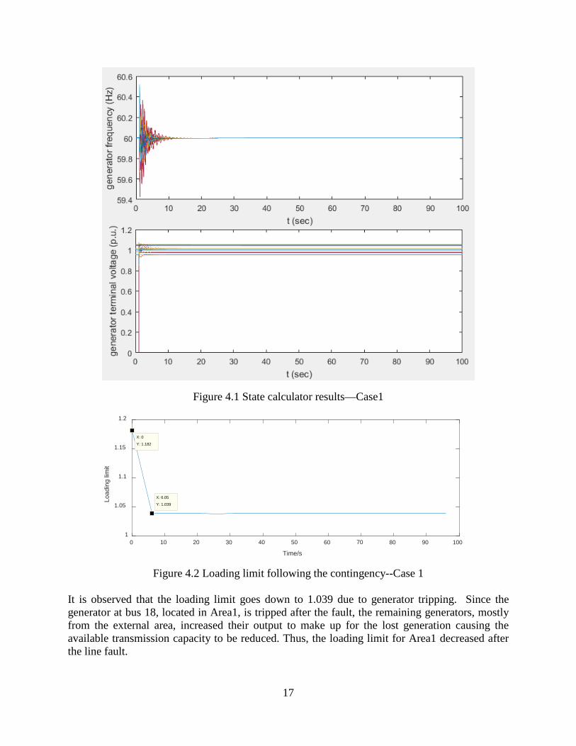
17

Figure 4.1 State calculator results—Case1

Figure 4.2 Loading limit following the contingency--Case 1

It is observed that the loading limit goes down to 1.039 due to generator tripping. Since the generator at bus 18, located in Area1, is tripped after the fault, the remaining generators, mostly from the external area, increased their output to make up for the lost generation causing the available transmission capacity to be reduced. Thus, the loading limit for Area1 decreased after the line fault.

0 10 20 30 40 50 60 70 80 90 100

Time/s

1

1.05

1.1

1.15

1.2

Load

ing

limit

X: 6.05

Y: 1.039

X: 0

Y: 1.182

18

Simulation results of Case 2

The SC results are shown in Figure 4.3. It is observed that the system tends to be stable after tripping the line 82-95. Incorporating the results of SC, the OPF-LI for Area1 is calculated every 5 seconds, and the results are shown in Figure 4.4.

Figure 4.3 State calculator results—Case 2 As shown in Figure 4.4, the load margin of Area1 decreases to 1.011 after the line fault on Line 82-95. Line 82-95 inside Area1. The Ward-PV equivalent system is updated based on the change of system topology. Since a line is tripped, the line flow constraint of Line 82-95 no longer applies, furthermore the line flow for other lines will increase, causing the loading limit to be reduced. Although the system is stable, the reduced loading limit obtained by OPF-LI indicates that the system is stressed after the fault.

19

Figure 4.4 Loading limit during the contigency--Case 2

4.4 4.4 Summary

Utilizing the PMU measurements and the SC, the loading limit can be estimated based on limited PMU data from only a few buses. The predictor-corrector method of SC does not require iterations. Thus, it is faster than the implicit integration method. Also, the network reduction algorithm Ward-PV is included in the process for estimation of the load margin. Hence the proposed approach is a promising tool to meet the requirement of an on-line application.

0 10 20 30 40 50 60 70 80 90 100

Time/s

1

1.05

1.1

1.15

1.2

Load

ingl

imit

X: 6.05

Y: 1.011

X: 0

Y: 1.185

20

5. OPF-LI with OLTC control

5.1 5.1 OLTC dynamic mechanism

OLTC model

One of the key mechanisms in load restoration is the voltage regulation performed automatically by the tap changing devices of power transformers. The tap changer controls the voltage magnitude of the secondary side 𝑉𝑉2 by changing the transformer ratio r, as Figure 5.1 shows.

Figure 5.1 Equivalent circuit of a tap transformer Practically, the tap positions are discrete and the OLTC is acting slowly because of the mechanical time delay and intentional time delay. A discrete model is [9]:

The LTC can operate at discrete time instants denoted by 𝑉𝑉𝑘𝑘, 𝑘𝑘 = 0,1, …

𝑉𝑉𝑘𝑘+1 = 𝑉𝑉𝑘𝑘 + Δ𝑇𝑇𝑘𝑘 (13)

Δ𝑇𝑇𝑘𝑘 is not necessarily constant

Δ𝑇𝑇𝑘𝑘 = 𝑇𝑇𝑓𝑓𝑖𝑖

|𝑉𝑉2 − 𝑉𝑉20|+ 𝑇𝑇𝑓𝑓 + 𝑇𝑇𝑚𝑚 (14)

𝑇𝑇𝑓𝑓 is the maximum time delay of the inverse-time characteristic; 𝑇𝑇𝑓𝑓"is the fixed intentional time delay, 𝑇𝑇𝑀𝑀 is the mechanical time.

𝑟𝑟𝑘𝑘+1 = �𝑟𝑟𝑘𝑘 + Δ𝑟𝑟 𝑖𝑖𝑓𝑓 𝑉𝑉2 > 𝑉𝑉2𝑡𝑡 + 𝑖𝑖 𝑉𝑉𝑖𝑖𝑖𝑖 𝑟𝑟𝑘𝑘 < 𝑟𝑟𝑚𝑚𝑟𝑟𝑘𝑘 − Δ𝑟𝑟 𝑖𝑖𝑓𝑓 𝑉𝑉2 < 𝑉𝑉2𝑡𝑡 + 𝑖𝑖 𝑉𝑉𝑖𝑖𝑖𝑖 𝑟𝑟𝑘𝑘 > 𝑟𝑟𝑚𝑚

𝑟𝑟𝑘𝑘 𝑙𝑙𝑉𝑉ℎ𝑒𝑒𝑟𝑟𝑒𝑒𝑖𝑖𝑉𝑉𝑒𝑒 (15)

1V 1 /V r2V

2 2,QP:1r

idealtransformer

tjX

21

For an analytical study, the following continuous model is adopted.

The continuous OLTC model is based on the assumption of a continuously changing tap (𝑉𝑉), which can take all real values between 𝑟𝑟𝑚𝑚𝑖𝑖𝑛𝑛 𝑉𝑉𝑖𝑖 𝑟𝑟𝑚𝑚𝑠𝑠𝑥𝑥.

𝑖𝑖𝑟𝑟𝑖𝑖𝑉𝑉

=1𝑇𝑇

(𝑉𝑉2 − 𝑉𝑉20) 𝑟𝑟𝑚𝑚𝑖𝑖𝑛𝑛 ≤ 𝑟𝑟 ≤ 𝑟𝑟𝑚𝑚𝑠𝑠𝑥𝑥 (16)

r is the tap ratio, T is time constant. The continuous LTC model is less accurate than discrete ones, but it is useful approximation, particularly convenient for analytical purposes.

OLTC dynamic mechanism for a simple system

By utilizing the continuous OLTC model presented before, the stability analysis for a simple power system is investigated in [16], as Figure 5.2 shows.

Figure 5.2 A simple power system with an OLTC For this system, the load voltage is described by

𝑉𝑉2 =𝐸𝐸

𝑍𝑍𝐿𝐿 + 𝑍𝑍/𝑖𝑖2∗𝑍𝑍𝑖𝑖

=𝑖𝑖𝐸𝐸𝑍𝑍

𝑖𝑖2𝑍𝑍𝑒𝑒 + 𝑍𝑍 (17)

Based on the load voltage and tap changer continuous model, the dynamic system equation can be obtained as

𝑖𝑖𝑖𝑖𝑖𝑖𝑉𝑉

=1𝑇𝑇

(𝑉𝑉𝑡𝑡 −𝑖𝑖𝐸𝐸𝑍𝑍

[𝑖𝑖4𝑍𝑍𝑒𝑒2 + 2𝑖𝑖2𝑍𝑍𝑍𝑍𝑒𝑒 cos(𝜃𝜃𝑒𝑒 − 𝜃𝜃) + 𝑍𝑍2]0.5) (18)

Based on the two equations, the relationship between 𝑖𝑖𝑖𝑖/𝑖𝑖𝑉𝑉 and n can be determined, also 𝑉𝑉2 and n. As shown in Figure 5.3, the equilibrium points 𝑖𝑖10,𝑖𝑖20 divide the tap positions into three intervals. Based on the sign of 𝑖𝑖𝑖𝑖/𝑖𝑖𝑉𝑉 in the intervals (0,𝑖𝑖10), (𝑖𝑖10, 𝑖𝑖20), (𝑖𝑖20,∞), the dynamic behavior of the tap changer can be illustrated in 5.3 (c).

LZ

E

LI1: n

Z1V 2V

22

Hence the region of attraction is (0,𝑖𝑖20), the stable equilibrium is 𝑖𝑖10. In case the tap position is beyond 𝑖𝑖20, n will increase since 𝑓𝑓𝑛𝑛

𝑓𝑓𝑡𝑡> 0, however load voltage 𝑉𝑉2 falls down, which will serve

as a cause for voltage collapse. Figure 5.3(d) shows the dynamic behavior for an OLTC in a discrete model, similar with the continuous model in Figure 5.3(c).

Figure 5.3 Dynamic mechanism for one OLTC system

OLTC dynamic mechanism for power system with M OLTCs

Generalizing the stability analysis presented before to a power system with M OLTCs, the system can be modeled by a differential-algebraic system as follows:

�̇�𝑖 = 𝑓𝑓(𝑖𝑖,𝑦𝑦,𝑝𝑝)

0 = 𝑙𝑙(𝑖𝑖,𝑦𝑦,𝑝𝑝) (19)

where 𝑖𝑖 ∈ 𝑋𝑋𝑛𝑛 represents the dynamic state variables, i.e., generator voltages and rotor phases, 𝑦𝑦 ∈𝑌𝑌𝑚𝑚 are the other variables, i.e., bus voltages and other rotor flow variables. The parameter space P is composed of system parameters, e.g., the system topology, and transformer ratios. Focusing

dn/dt

7(a)N

7(b)

7(c)

7(d)

10n 20n

10n 20n

10n 20n

1e 2e

V ′

0

0

n

n

n

n

Region of attraction

23

on tap changer dynamics, the time scale is longer than that corresponding to generator dynamics, therefore it is acceptable to neglect the transient dynamics �̇�𝑖, by

0 = 𝑓𝑓(𝑖𝑖, 𝑦𝑦,𝑝𝑝) (20)

Incorporating the continuous model for OLTC, the equilibrium points for the system model will be found by solving

�

𝑖𝑖𝑟𝑟𝑖𝑖𝑉𝑉

=Δ𝑉𝑉𝑇𝑇

= 0

𝑓𝑓(𝑖𝑖,𝑦𝑦) = 0𝑙𝑙(𝑖𝑖,𝑦𝑦, 𝑟𝑟) = 0

(21)

For a nonlinear system, linearization is performed around each equilibrium. Then Jacobian A will be used to determine whether this equilibrium is stable or not. However, since the system model is much more complex for a system with M OLTCs, there should be multiple equilibrium points. It will be difficult to calculate the regions of attraction. Therefore, a direct way is to describe the voltage recovery region. The voltage recovery region [15] is an area in which all bus voltages will go up with respect to time when there is a low voltage condition.

5.2 OLTC operating control

In order to improve the power system operating condition, the proposed OLTC operating control is presented blow, where k denotes the time step.

OLTC Operation:

tap(k)-tap(k-1) = 0/-1/1 tap− ≤ tap(𝑘𝑘) ≤ tap+ (22) If 𝑉𝑉(𝑘𝑘) − 𝑉𝑉𝑟𝑟𝑒𝑒𝑓𝑓 ≥ Δ𝑉𝑉𝑟𝑟𝑒𝑒𝑓𝑓

𝑉𝑉𝑉𝑉𝑝𝑝(𝑘𝑘 + 1) − 𝑉𝑉𝑉𝑉𝑝𝑝(𝑘𝑘) = 1 (23) Else if 𝑉𝑉(𝑘𝑘) − 𝑉𝑉𝑟𝑟𝑒𝑒𝑓𝑓 ≤ −Δ𝑣𝑣𝑟𝑟𝑒𝑒𝑓𝑓

𝑉𝑉𝑉𝑉𝑝𝑝(𝑘𝑘 + 1) − 𝑉𝑉𝑉𝑉𝑝𝑝(𝑘𝑘) = −1 (24) Else if �𝑉𝑉(𝑘𝑘) − 𝑉𝑉𝑟𝑟𝑒𝑒𝑓𝑓� < Δ𝑣𝑣𝑟𝑟𝑒𝑒𝑓𝑓

𝑉𝑉𝑉𝑉𝑝𝑝(𝑘𝑘 + 1) − 𝑉𝑉𝑉𝑉𝑝𝑝(𝑘𝑘) = 0 (25) OLTC blocking:

If 𝑉𝑉𝑉𝑉𝑝𝑝(𝑘𝑘) − 𝑉𝑉𝑉𝑉𝑝𝑝(𝑘𝑘 − 1) = −1 𝑉𝑉𝑁𝑁𝑃𝑃 𝑉𝑉(𝑘𝑘) − 𝑉𝑉(𝑘𝑘 − 1) ≤ 0

𝑉𝑉𝑉𝑉𝑝𝑝(𝑘𝑘 + 1) = 𝑉𝑉𝑉𝑉𝑝𝑝(𝑘𝑘) (26)

24

The principle for OLTC Operation is based on the discrete model of the OLTC. Furthermore, it is noted that the tap changer will be blocked as soon as Δ𝑉𝑉𝑉𝑉𝑝𝑝 < 0 𝑉𝑉𝑖𝑖𝑖𝑖 Δ𝑉𝑉 < 0. In other words, although the tap changer tries to raise the load side voltage to correct the deviation of load voltage from the set point, the voltage magnitude can still decreases due to the limitation of the OLTC control principle. Based on the analysis for the voltage recovery region, the criteria of OLTC blocking is developed. By utilizing the relation between Δtap and ΔV, OLTC blocking control is implemented.

5.3 OPF-LI with OLTC control

The proposed approach OPF-LI is used to estimate the loading limit for a load area by the OPF based algorithm. The optimization is subject to the network constraint and some inequality constraints. Base on the proposed OLTC control strategies, the dynamics of OLTC are incorporated to modify the loading limit. The flowchart is shown in Figure 5.4.

Figure 5.4 OPF-LI with OLTC operating control The flowchart in Figure 5.4 illustrates the procedure to estimate the loading limit with the effect of OLTC operating control introduced in Section 5.2. The WECC 179 bus system is used for testing. The detailed procedure is given below:

Step1: Calculate the loading limit 𝜆𝜆𝑚𝑚𝑠𝑠𝑥𝑥 for the base case loading. Step2: Using 𝜆𝜆𝑚𝑚𝑠𝑠𝑥𝑥 as the initial load ratio 𝜆𝜆0 to update the loading, the operation of OLTC

is triggered. Step3: Calculate the OPF-LI with the updated system states after the OLTC operation.

25

Step4: Compare OPF-LI solution with the criteria. If loading margin is still available, 𝜆𝜆 should go up for the next iteration. On the other hand, if the loading margin is close to 0 so that the OPF algorithm cannot converge, 𝜆𝜆 will decrease for the next iteration. It is indicated that the loading limit is not final once λ is modified.

Step5: Back to Step1 and recalculate the OPF-LI. Step6: Determine the loading limit incorporating the OLTC control. Once OPF-LI solution

falls below the setting limit 1.02, the load ratio 𝜆𝜆𝑛𝑛 will be the value which is the actual loading limit.

5.4 Simulation results

The WECC 179 bus system is used to implement the proposed OLTC operating control. Assume that the load of Area1 increases to 1.18 times from the base case loading. Because of the load increase, OLTCs are triggered by the voltage deviation. The simulation results are shown Figure 5.5, Figure 5.6.

Blue curve: voltage profile of the voltage reference;

Red cure: voltage profile at the beginning of tap operation;

Green cure: voltage profile with OLTC blocking control.

X axis: Bus number of 179 bus system

Y axis: Voltage magnitude

Figure 5.5 Comparison of voltage profiles—without OLTC blocking control

0 20 40 60 80 100 120 140 160 180

Bus number

0.6

0.7

0.8

0.9

1

1.1

1.2

Volta

ge m

agni

tude

/p.u

.

ref

beforetap

aftertap

26

Figure 5.6 Comparison of voltage profiles—with OLTC blocking control

Table 5-1 Comparison of voltage magnitude for blocked bus

Bus number V before tap operation

V after tap operation (without OLTC

blocking)

V after tap operation

(with OLTC blocking)

Voltage change

(without OLTC

blocking)

Voltage change (with

OLTC blocking)

46 1.0348 0.9301 1.0069 -0.1047

-0.0279 47 1.0200 1.0200 1.0200 0 0 48 1.0340 0.9295 1.0054 -0.1045

-0.0286 50 1.0236 0.9153 1.0079 -0.1083

-0.0157 53 1.0366 0.9367 1.0281 -0.0999

-0.0085 Figure 5.5 illustrates that the voltage profile for the 179-bus system, represented by the green curve, is not improved after the tap operation. It is observed that the voltage of most buses drops comparing with the red curve. Without OLTC blocking, the tap changing cause the voltage drops when the operating point falls out of the recovery region. In this case, some tap changers are blocked at the maximal position when the tap ratio reaches the upper or lower limits, so that the system condition does not collapse deteriorate.

As shown in the green curve in Figure 5.6, the voltage profile is improved due to OLTC blocking control. Along with the operation, OLTCs located at transformer buses 46, 47, 48 ,50, 53 are blocked based on the criteria discussed in the previous section. By doing so, the dynamic behavior of OLTC is improved and the system condition is restored without having a voltage collapse.

It is observed from Table 5-1 that the voltages at the blocked buses (46, 47, 48 ,50, 53) decrease by 0.1 p.u. after the OLTC operation since no blocking control is adopted. The voltage change for the case with OLTC blocking shows that the blocking strategy prevents these critical buses from a collapse.

0 20 40 60 80 100 120 140 160 180

Bus number

0.9

0.95

1

1.05

1.1

1.15

1.2

Volta

ge m

agni

tude

/p.u

ref

beforetapaftertap

27

Table 5-2 Comparison of base case load case and light load case

Base case load case Light load case (Reduce heavy load for 10%)

OPF-LI without OLTC blocking control 1.1742 1.5090

OPF-LI after OLTC blocking control 1.2742 1.7890

The number of blocked taps 5 1

As shown in Table 5-2 shows, for the base case loading, the loading limit estimated by the original OPF-LI is 1.1742. Then the loading limit increases to 1.2742 with the OLTC blocking. OLTC as a critical device can regulate the load voltage efficiently, hence the loading margin will increase. However, the base case loading of the WECC system is heavy. Some of the taps changers are blocked to prevent instability during the operation. That is why the loading limit can only increase by 0.1 with respect to the line flow constraints and the generation constraints. To investigate the performance of the proposed OLTC blocking control, a heavy load scenario with more than 2000 MVA in the 179 bus system is reduced by 10%. In this case, the loading limit before tap is 1.5090. However, the loading limit is modified to 1.7890 after the OLTC blocking control. Since the system is not as stressed as the base case, only one tap changer is blocked when the load is increased to 1.789.

5.5 Summary

Based on the dynamic mechanism of OLTCs, an OTLC blocking control is proposed. The OTLC blocking control can prevent these critical buses from unstable operating conditions. OPF-LI is modified to incorporate the proposed OLTC control and, as a result, the loading limit has been improved. By utilizing the relation between Δtap and ΔV, the proposed OLTC blocking strategy prevents the undesirable tap changes once the position falls within an unstable condition.

28

6. Conclusions

In this project, two methods VSAI and OPF-LI are proposed for the assessment of long-term voltage stability for power systems. This work includes four parts:

1) VSAI is a Thevenin Equivalent based indictor. By estimating the Thevenin impedance at a load bus, the index can indicate whether the system at this operation point is stable or not. However, it may not be accurate as the system model is radically simplified into a two-node system.

2) To extend the TE-based model from a 2-node model to a multiple bus model, a new method to estimate the loading limit for a load center is developed which includes the Ward-PV equivalent and an OPF based algorithm. By the Ward-PV equivalent, the network reduction can be obtained so that the computational speed for the optimization will be high. OPF-LI approximates the loading margin for the load area.

3) In order to utilize the limited number of available PMUs, the State Calculator is used to approximate the system states in an on-line environment. OPF-LI with SC can estimate the loading limit based on the limited PMU data. The predictor-corrector method of SC does not require iterations. Thus, it is faster than the implicit integration method. Also, the network reduction algorithm Ward-PV is included in the process estimating the load margin. Hence, the proposed approach is efficient.

4) Since the solution of OPF-LI is derived from power flow constraints, the dynamic mechanism of OLTC should be incorporated to obtain a realistic optimal solution. A novel OTLC blocking control is proposed. The OTLC blocking control can prevent these critical buses from unstable operating conditions. The loading limit incorporating the proposed OLTC blocking control is an improved index. Utilizing the relation between Δtap and ΔV, the new OLTC blocking strategy can prevent undesirable tap operations once the position falls under unstable conditions.

29

References

[1] K. T. Vu, C. C. Liu, C. W. Taylor and K. M. Jimma, "Voltage instability: mechanisms and control strategies [power systems]," Proceedings of the IEEE, vol. 83, no. 11, pp. 1442-1455, Nov 1995.

[2] T. Cutsem and C. Vournas, Voltage stability of electric power systems. New York: Springer, 2008.

[3] K. Vu, M. M. Begovic, D. Novosel and M. M. Saha, "Use of local measurements to estimate voltage-stability margin," in IEEE Transactions on Power Systems, vol. 14, no. 3, pp. 1029-1035, Aug 1999.

[4] I. Smon, G. Verbic and F. Gubina, "Local voltage-stability index using tellegen's Theorem," in IEEE Transactions on Power Systems, vol. 21, no. 3, pp. 1267-1275, Aug. 2006.

[5] S. Corsi and G. N. Taranto, "A Real-Time Voltage Instability Identification Algorithm Based on Local Phasor Measurements," in IEEE Transactions on Power Systems, vol. 23, no. 3, pp. 1271-1279, Aug. 2008.

[6] F. Hu, K. Sun, A. Del Rosso, E. Farantatos and N. Bhatt, "Measurement-Based Real-Time Voltage Stability Monitoring for Load Areas," in IEEE Transactions on Power Systems, vol. 31, no. 4, pp. 2787-2798, July 2016.

[7] B. Gao, G. K. Morison and P. Kundur, "Voltage stability evaluation using modal analysis," in IEEE Transactions on Power Systems, vol. 7, no. 4, pp. 1529-1542, Nov 1992.

[8] V. Ajjarapu and C. Christy, "The continuation power flow: a tool for steady state voltage stability analysis," in IEEE Transactions on Power Systems, vol. 7, no. 1, pp. 416-423, Feb 1992.

[9] N. Flatabo, R. Ognedal and T. Carlsen, "Voltage stability condition in a power transmission system calculated by sensitivity methods," in IEEE Transactions on Power Systems, vol. 5, no. 4, pp. 1286-1293, Nov 1990.

[10] F. Capitanescu and T. Van Cutsem, "Unified sensitivity analysis of unstable or low voltages caused by load increases or contingencies," in IEEE Transactions on Power Systems, vol. 20, no. 1, pp. 321-329, Feb. 2005.

[11] R. S. Diao, K. Sun, V. Vittal, R. O'Keefe, M. Richardson, N. Bhatt, D. Stradford and S. Sarawgi, "Decision Tree-Based Online Voltage Security Assessment Using PMU Measurements", IEEE Transactions on Power Systems, vol. 24, no. 2, pp. 832-839, 2009.

[12] S. S. Biswas and A. K. Srivastava, "Voltage Stability Monitoring in Power Systems, " U.S. Patent, Feb. 25, 2014

[13] F. Wu and A. Monticelli, "Critical review of external network modelling for online security analysis", International Journal of Electrical Power & Energy Systems, vol. 5, no. 4, pp. 222-235, 1983.

[14] G. Wang, C. C. Liu, N. Bhatt, E. Farantatos and M. Patel, "Observability of nonlinear power system dynamics using synchrophasor data", International Transactions on Electrical Energy Systems, vol. 26, no. 5, pp. 952-967, 2015.

[15] K. Vu and C. C. Liu, "Dynamic mechanisms of voltage collapse", Systems & Control Letters, vol. 15, no. 4, pp. 329-338, 1990.

[16] C. C. Liu and K. Vu, "Analysis of tap-changer dynamics and construction of voltage stability regions," in IEEE Transactions on Circuits and Systems, vol. 36, no. 4, pp. 575-590, Apr 1989.