Wavefront Sensing II

Richard Lane

Department of Electrical and Computer Engineering

University of Canterbury

Contents

• Session 1 – Principles

• Session 2 – Performances

• Session 3 – Wavefront Reconstruction

Session 2 Performances

• Geometrical wavefront sensing take 2

• The inverse problem

• The astronomical setting

• The basic methods

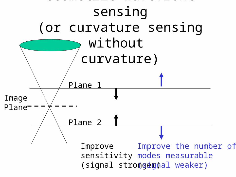
Geometric wavefront sensing(or curvature sensing without

curvature)

Plane 1

Plane 2

ImagePlane

Improve sensitivity(signal stronger)

Improve the number of modes measurable(signal weaker)

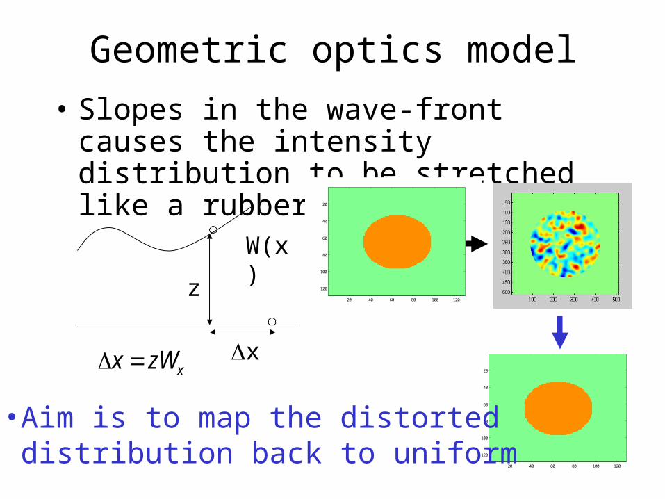
• Slopes in the wave-front causes the intensity distribution to be stretched like a rubber sheet

Geometric optics model

z

W(x)

xxzWx

20 40 60 80 100 120

20

40

60

80

100

120

20 40 60 80 100 120

20

40

60

80

100

120

•Aim is to map the distorted distribution back to uniform

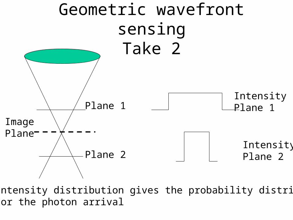
Geometric wavefront sensingTake 2

Plane 1

Plane 2

ImagePlane

Intensity Plane 1

Intensity Plane 2

Intensity distribution gives the probability distributionFor the photon arrival

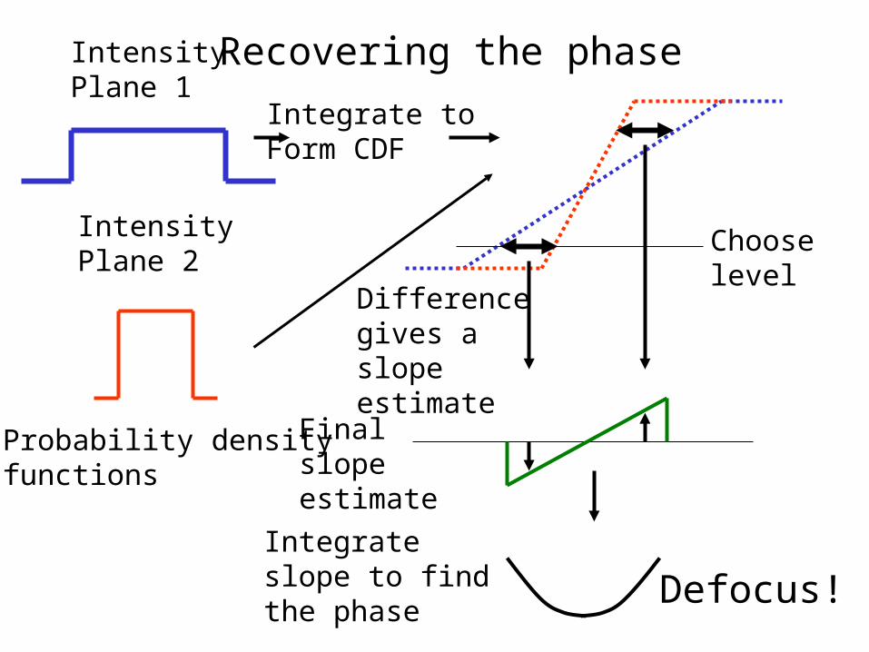
Intensity Plane 1

Intensity Plane 2

Probability densityfunctions

Integrate toForm CDF

Chooselevel

Difference gives a slope estimate

Finalslope estimate

Integrateslope to findthe phase

Recovering the phase

Defocus!

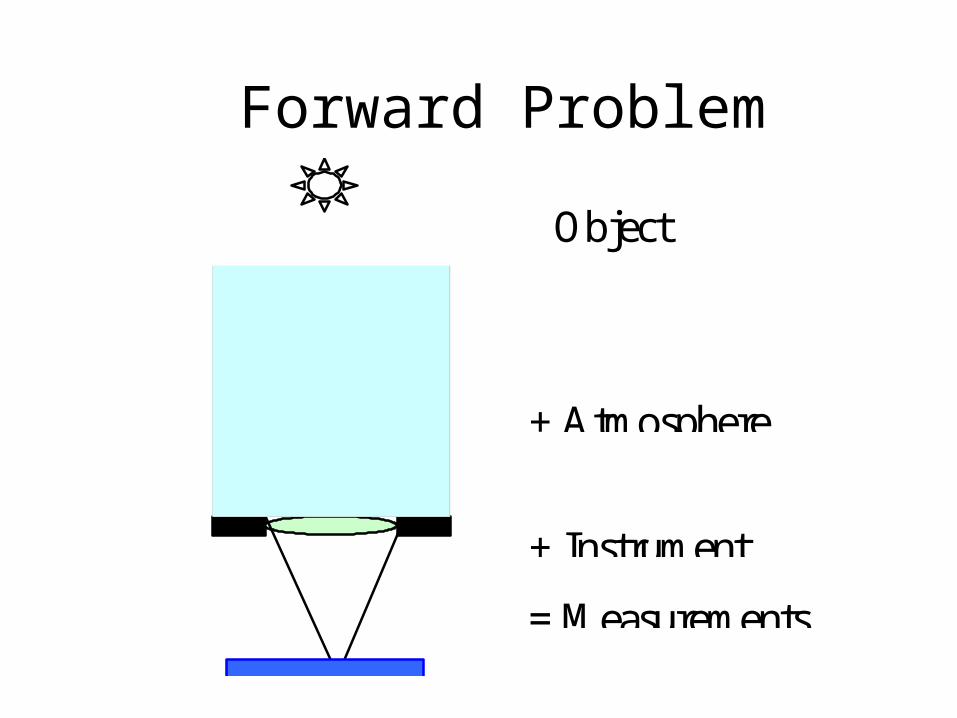
Forward Problem

Object

+ Atmosphere

= Measurements

+ Instrument

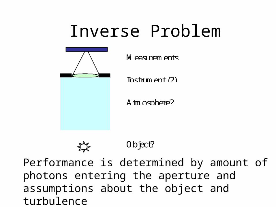
Inverse Problem

Object?

Atmosphere?

Measurements

Instrument (?)

Performance is determined by amount of photons entering the aperture and assumptions about the object and turbulence

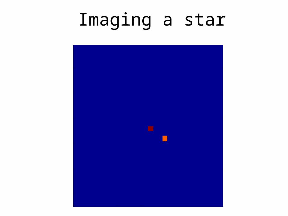
Imaging a star  

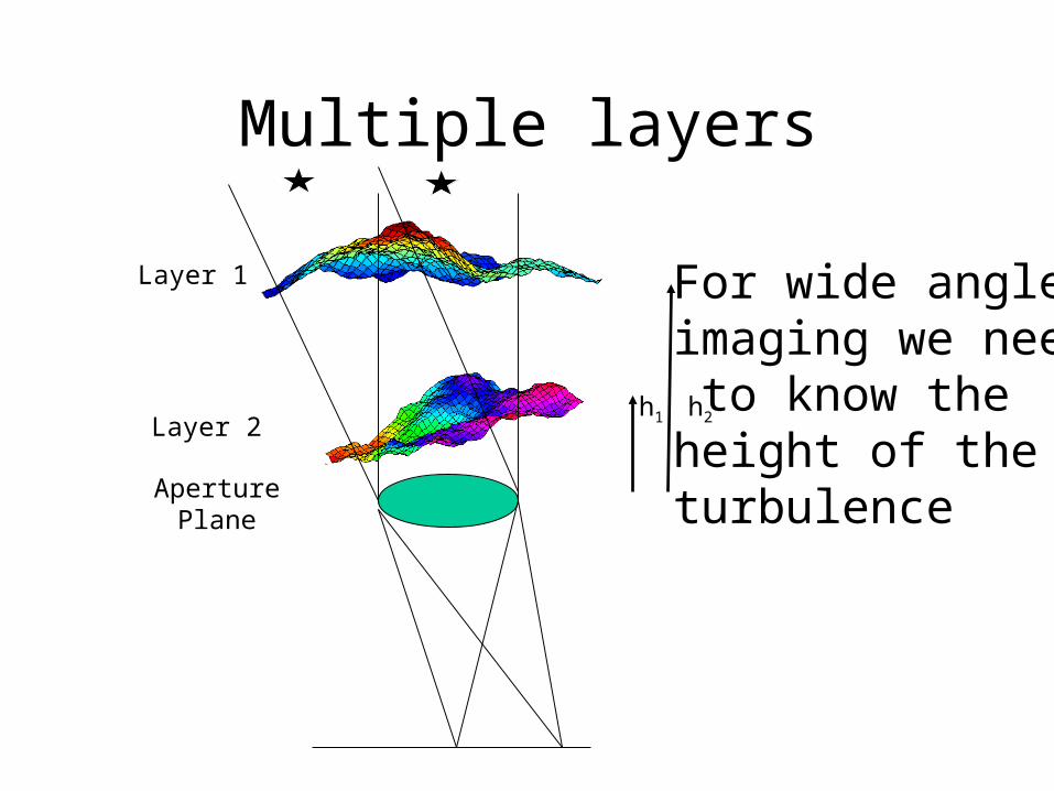
Multiple layers

Layer 1

Layer 2

AperturePlane

h1 h2

For wide angleimaging we need to know the height of the turbulence

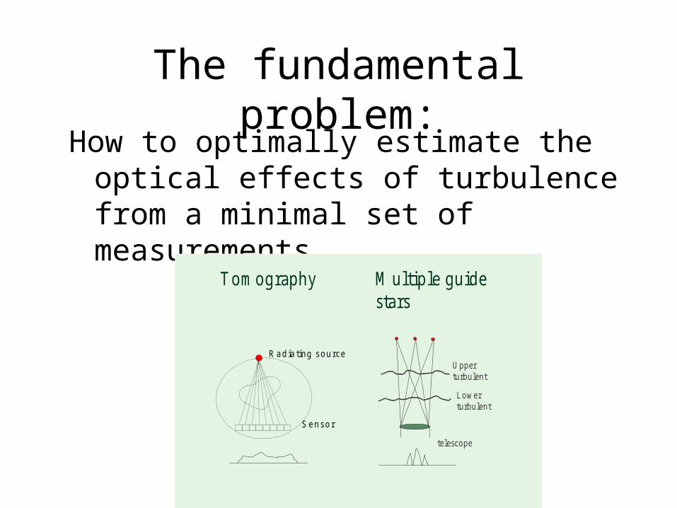
The fundamental problem:How to optimally estimate the optical effects

of turbulence from a minimal set of measurements

T o m o g ra p h y M u ltip le g u id e s ta rs

R ad ia ting source

S ensor

te le sc o p e

U p p e rtu rb u le n t

L o w e rtu rb u le n t

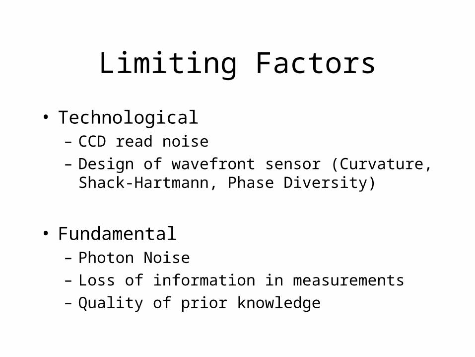
Limiting Factors

• Technological – CCD read noise

– Design of wavefront sensor (Curvature, Shack-Hartmann, Phase Diversity)

• Fundamental – Photon Noise

– Loss of information in measurements

– Quality of prior knowledge

In Its Raw Form the Inverse Problem Is Always Insoluble

• There are always an infinite number of ways to explain data.

• The problem is to explain the data in the most reasonable way

• Example Shack-Hartmann sensing for estimating turbulence

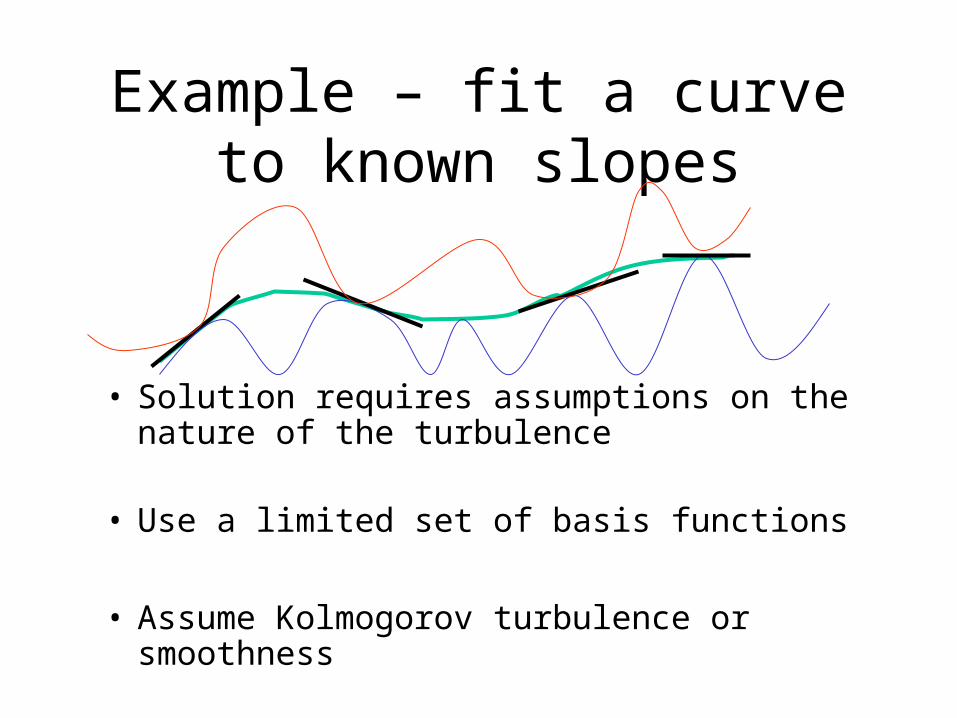
Example – fit a curve to known slopes

• Solution requires assumptions on the nature of the turbulence

• Use a limited set of basis functions

• Assume Kolmogorov turbulence or smoothness

Parameter estimation• Essentially we need to find a set of unknown

parameters which describe the object and/or turbulence

• The parameters can be in terms of pixels or coefficients of basis functions

• Solution should not be overly sensitive to our choice of parameters.

• Ideally it should be on physical grounds

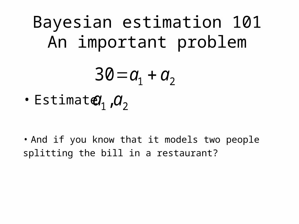
Bayesian estimation 101An important problem

• Estimate

• And if you know that it models two people

splitting the bill in a restaurant?

2130 aa

21 ,aa

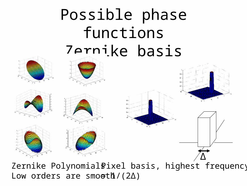
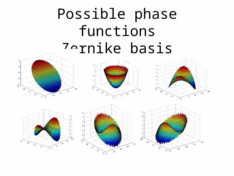
Possible phase functionsZernike basis

Zernike PolynomialsLow orders are smooth

Pixel basis, highest frequency= 1/(2Δ)

Δ

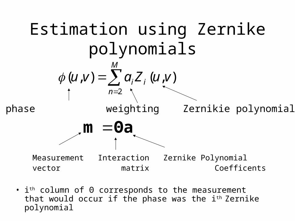
Estimation using Zernike polynomials

Measurement Interaction Zernike Polynomialvector matrix Coefficents

M

nii vuZavu

2

),(),(

Θam

• ith column of Θ corresponds to the measurement that would occur if the phase was the ith Zernike polynomial

phase weighting Zernikie polynomial

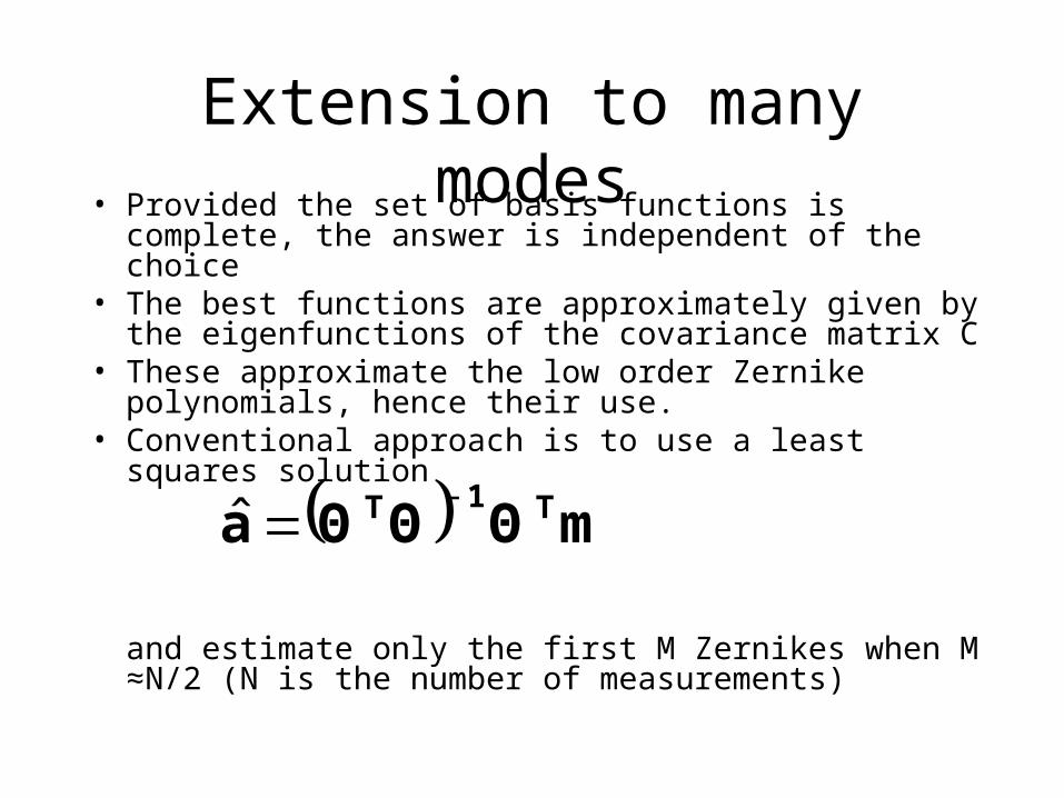
Extension to many modes• Provided the set of basis functions is complete, the answer

is independent of the choice• The best functions are approximately given by the

eigenfunctions of the covariance matrix C• These approximate the low order Zernike polynomials,

hence their use.• Conventional approach is to use a least squares solution

and estimate only the first M Zernikes when M ≈N/2 (N is

the number of measurements)

mΘΘΘa T1T ˆ

Not all measurements are equally noisy hence minimise

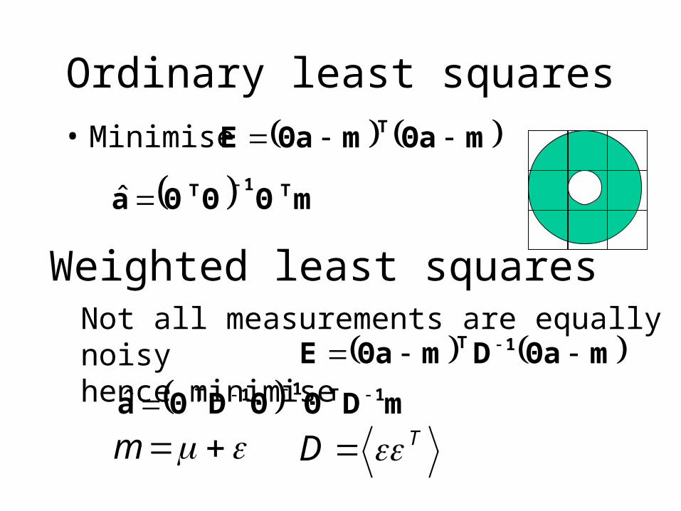
Ordinary least squares

• Minimise mΘamΘaE T

mΘΘΘa T1T ˆ

Weighted least squares

mΘaDmΘaE 1T

mDΘΘDΘa 1T11T ˆ

m TD

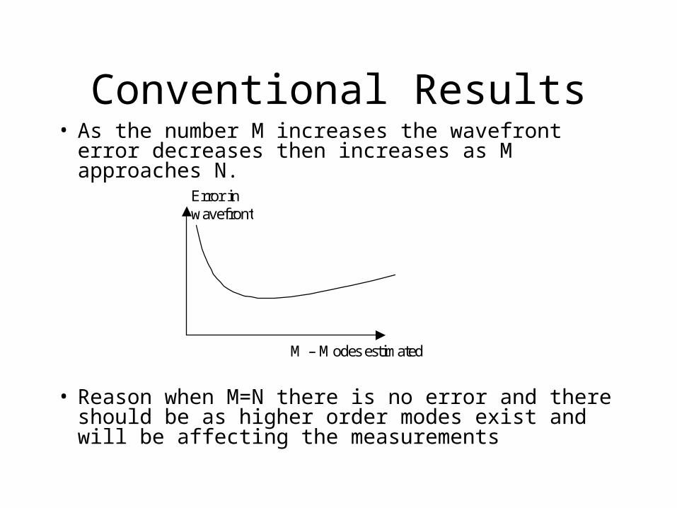
Conventional Results• As the number M increases the wavefront error

decreases then increases as M approaches N.

• Reason when M=N there is no error and there should be as higher order modes exist and will be affecting the measurements

M – Modes estimated

Error in wavefront

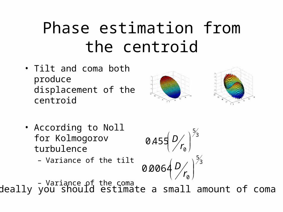
Phase estimation from the centroid

• Tilt and coma both produce displacement of the centroid

• According to Noll for Kolmogorov turbulence– Variance of the tilt

– Variance of the coma

35

0455.0

r

D

35

00064.0

r

D

Ideally you should estimate a small amount of coma

Bayesian viewpoint

• The problem in the previous slide is that we are not modelling the problem correctly

• Assuming that the higher order modes are zero, is forcing errors on the lower order modes

• Need to estimate the coefficients of all the modes as random variables

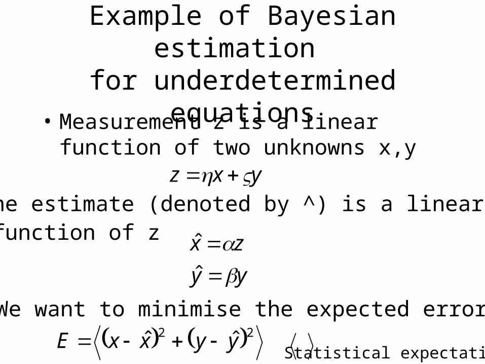
Example of Bayesian estimation for underdetermined equations

• Measurement z is a linear function of two unknowns x,y

yxz

yy

zx

ˆ

ˆ

22 ˆˆ yyxxE Statistical expectation

• We want to minimise the expected error

• The estimate (denoted by ^) is a linear function of z

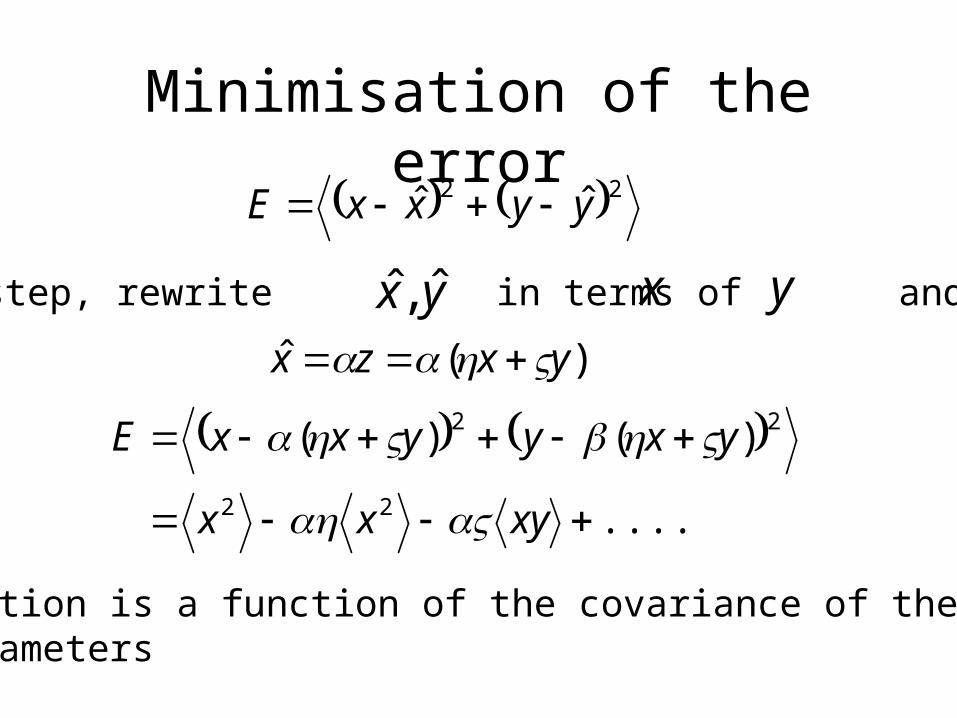
Minimisation of the error 22 ˆˆ yyxxE

•Key step, rewrite in terms of andyx ˆ,ˆ x

)(ˆ yxzx

y

....

)()(

22

22

xyxx

yxyyxxE

•Solution is a function of the covariance of the unknown parameters

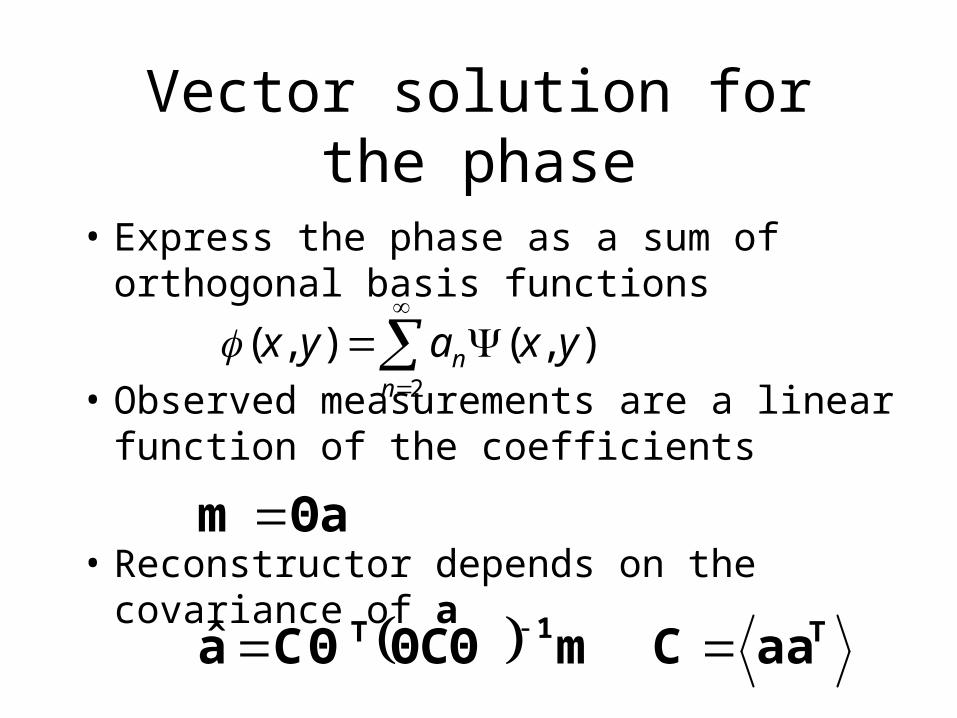
Vector solution for the phase

• Express the phase as a sum of orthogonal basis functions

• Observed measurements are a linear function of the coefficients

• Reconstructor depends on the covariance of a

2

),(),(n

n yxayx

Θam

mΘCΘCΘa 1T ˆ TaaC

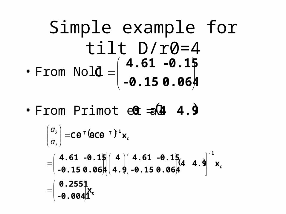
Simple example for tilt D/r0=4

• From Noll

• From Primot et al

0.0640.15-

0.15-4.61C

c

c

1

c

1TT

x0.0041-

0.2551

x4.940.0640.15-

0.15-4.61

4.9

4

0.0640.15-

0.15-4.61

xΘCΘCΘ

7

2

a

a

4.94Θ

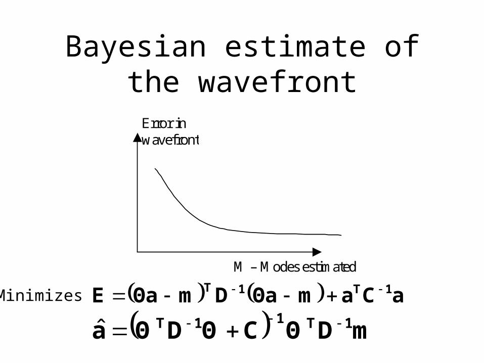
Bayesian estimate of the wavefront

M – Modes estimated

Error in wavefront

mDΘCΘDΘa 1T11T ˆ

aCamΘaDmΘaE 1T1T Minimizes

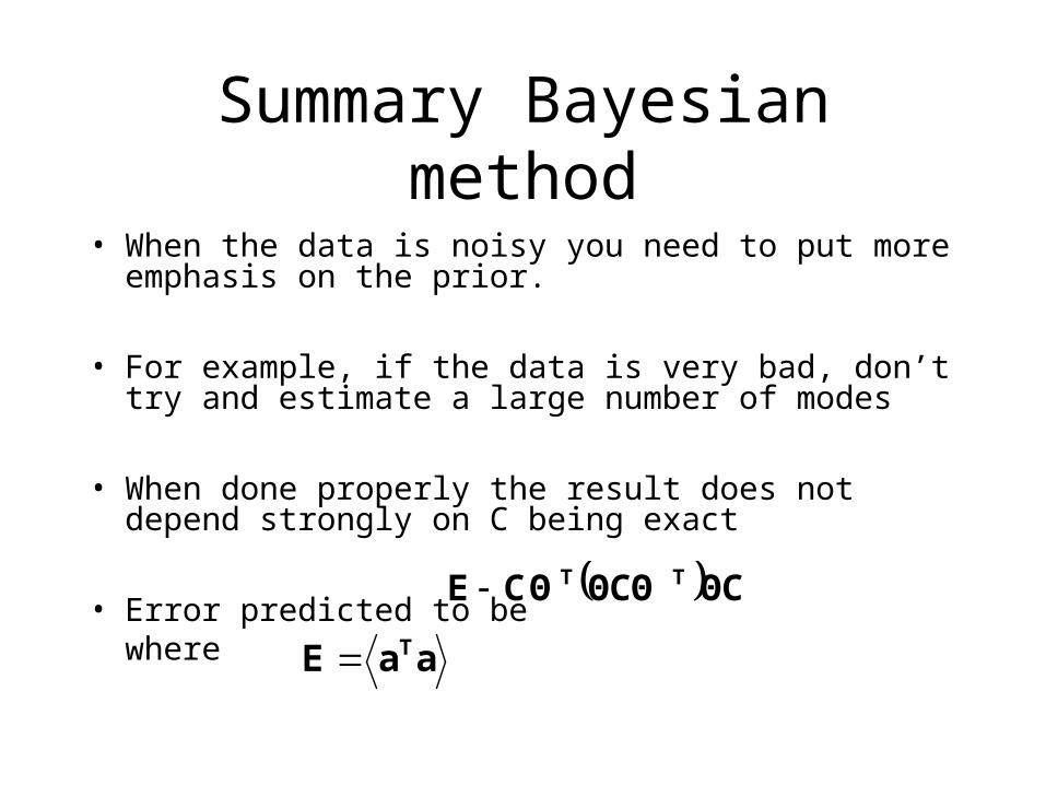
Summary Bayesian method

• When the data is noisy you need to put more emphasis on the prior.

• For example, if the data is very bad, don’t try and estimate a large number of modes

• When done properly the result does not depend strongly on C being exact

• Error predicted to be where

ΘCΘCΘCΘE TT

aaE T

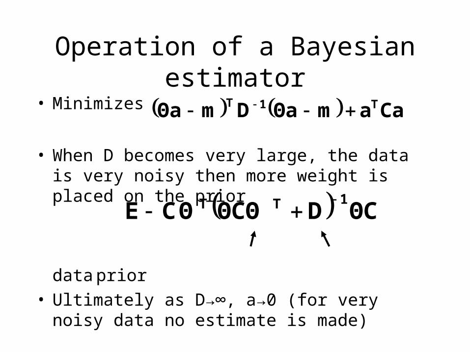
Operation of a Bayesian estimator

• Minimizes

• When D becomes very large, the data is very noisy then more weight is placed on the prior

data prior• Ultimately as D→∞, a→0 (for very noisy data no

estimate is made)

ΘCDΘCΘCΘE1TT

CaamΘaDmΘa T1T

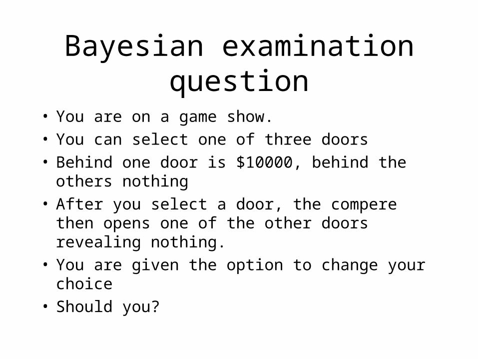
Bayesian examination question

• You are on a game show. • You can select one of three doors• Behind one door is $10000, behind the others

nothing• After you select a door, the compere then opens

one of the other doors revealing nothing.• You are given the option to change your choice • Should you?

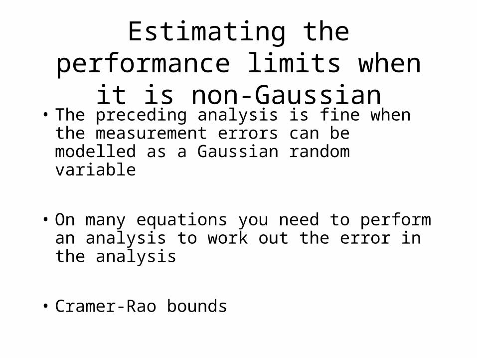
Estimating the performance limits when it is non-Gaussian

• The preceding analysis is fine when the measurement errors can be modelled as a Gaussian random variable

• On many equations you need to perform an analysis to work out the error in the analysis

• Cramer-Rao bounds

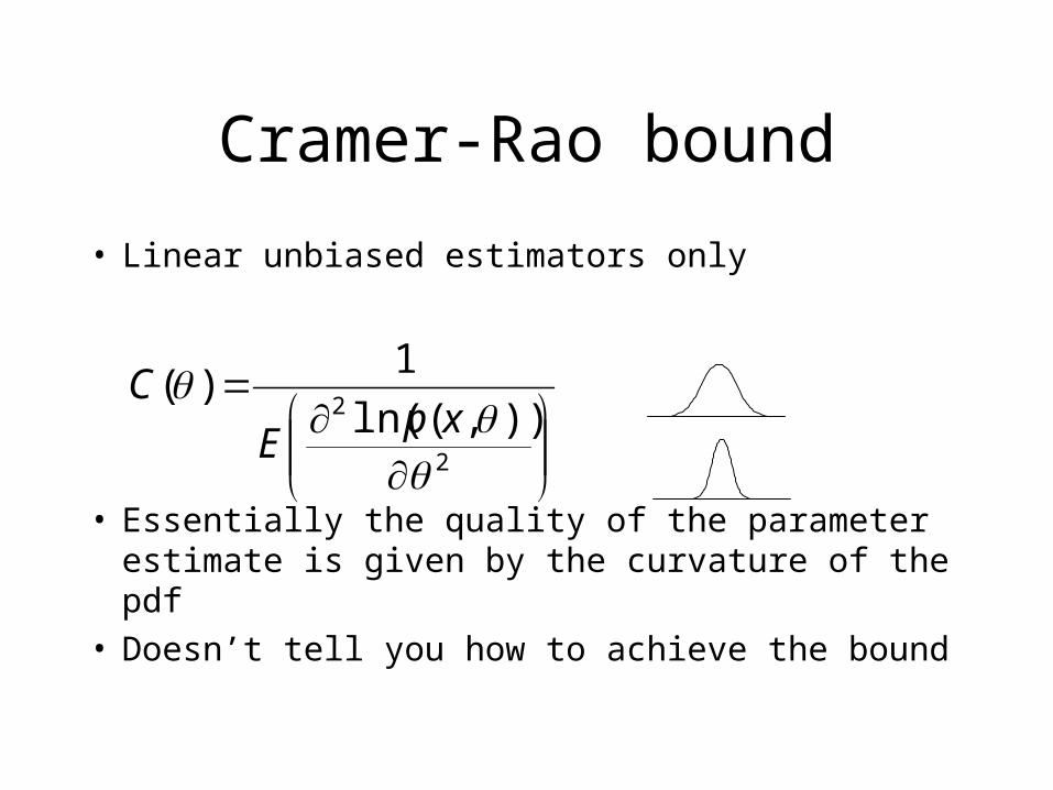
Cramer-Rao bound

• Linear unbiased estimators only

• Essentially the quality of the parameter estimate is given by the curvature of the pdf

• Doesn’t tell you how to achieve the bound

2

2 )),(ln(

1)(

xp

E

C

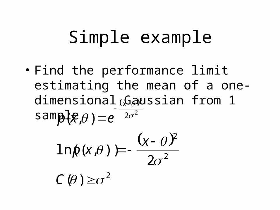
Simple example

• Find the performance limit estimating the mean of a one-dimensional Gaussian from 1 sample

2

2

2

2

)(

2)),(ln(

),(2

2

C

xxp

expx

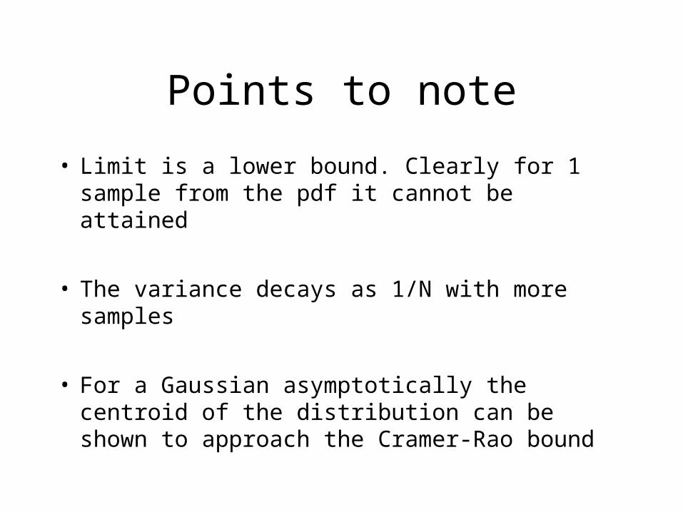
Points to note

• Limit is a lower bound. Clearly for 1 sample from the pdf it cannot be attained

• The variance decays as 1/N with more samples

• For a Gaussian asymptotically the centroid of the distribution can be shown to approach the Cramer-Rao bound

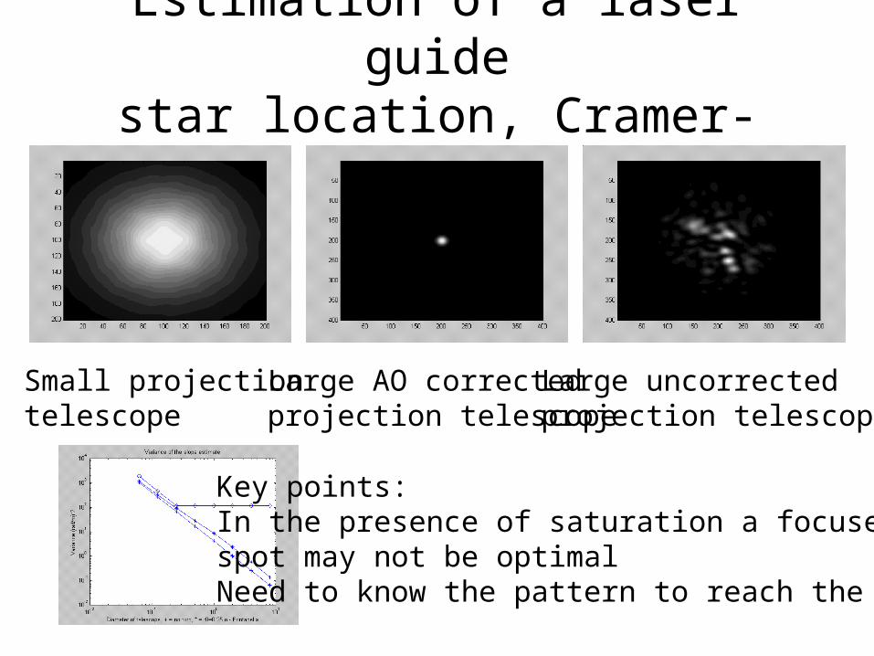
Estimation of a laser guidestar location, Cramer-Rao bound

Small projectiontelescope

Large AO corrected projection telescope

Large uncorrected projection telescope

Key points:In the presence of saturation a focused spot may not be optimalNeed to know the pattern to reach the limit

Optimal estimation of a parameterwavefront tilt

• Important because the wavefront tilt is the dominant form of phase aberration

• A small error in estimating the tilt can be larger than the full variance of a higher order aberration.

Issues

• Displacement of the centroid of an image is proportional to the average tilt (not the least mean square) of the phase distortion

• Will discuss this issue later, but for the moment concentrate on estimating the mean square tilt.

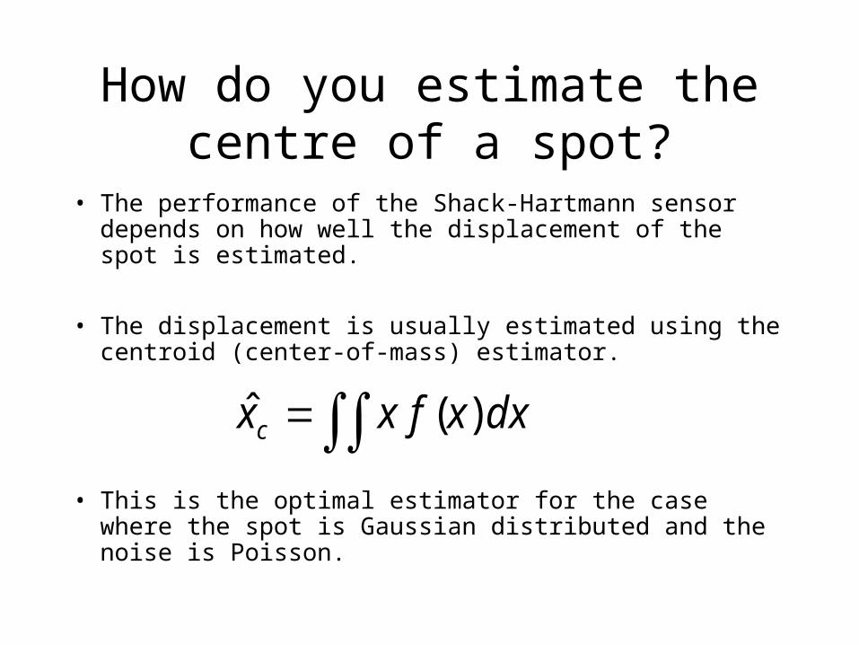
How do you estimate the centre of a spot?

• The performance of the Shack-Hartmann sensor depends on how well the displacement of the spot is estimated.

• The displacement is usually estimated using the centroid (center-of-mass) estimator.

• This is the optimal estimator for the case where the spot is Gaussian distributed and the noise is Poisson.

dxxfxxc )(ˆ

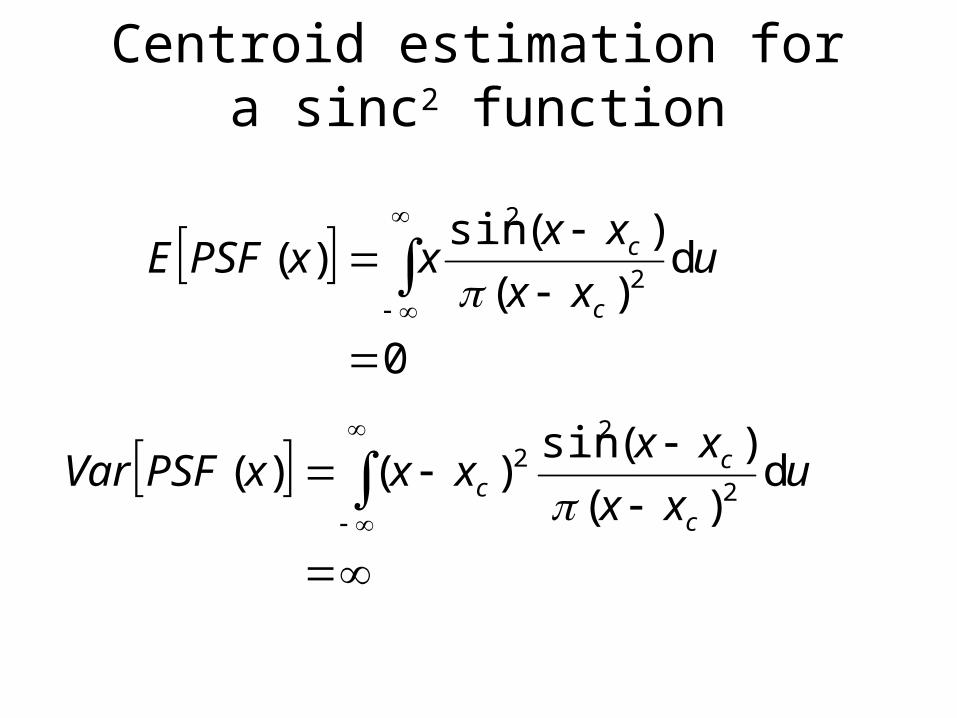
Centroid estimation for a sinc2 function

0

d)(

)(sin)(

2

2

uxx

xxxxPSFE

c

c

uxx

xxxxxPSFVar

c

cc d

)(

)(sin)()(

2

22

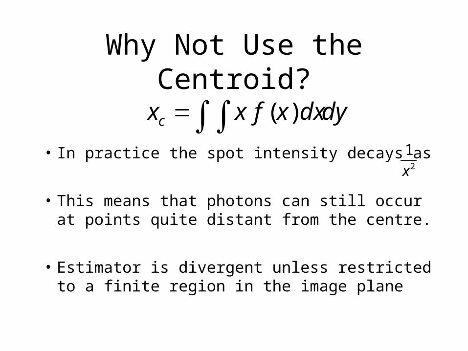
Why Not Use the Centroid?

• In practice the spot intensity decays as

• This means that photons can still occur at points quite distant from the centre.

• Estimator is divergent unless restricted to a finite region in the image plane

2

1

x

dydxxfxxc )(

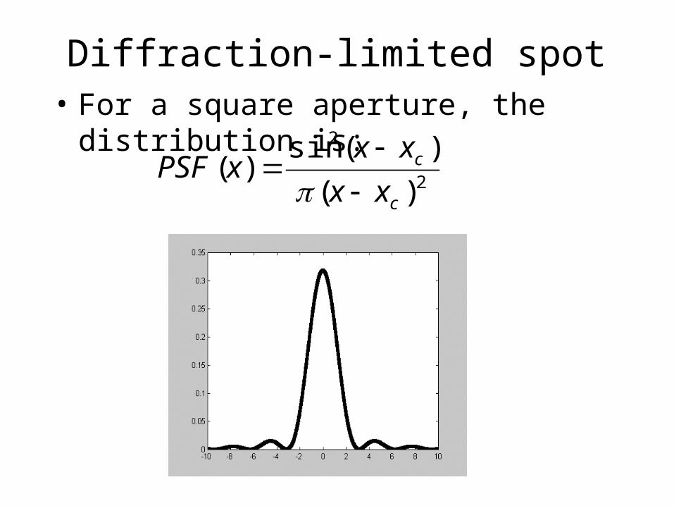
Diffraction-limited spot• For a square aperture, the distribution is:

2

2

)(

)(sin)(

c

c

xx

xxxPSF

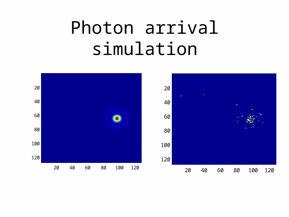
Photon arrival simulation

20 40 60 80 100 120

20

40

60

80

100

120

20 40 60 80 100 120

20

40

60

80

100

120

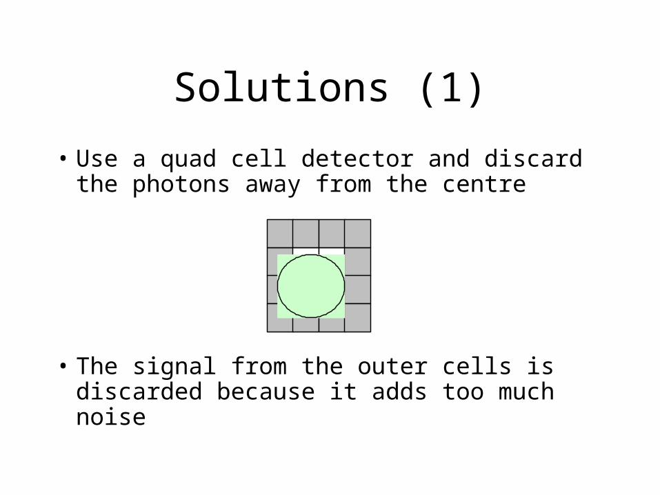
Solutions (1)

• Use a quad cell detector and discard the photons away from the centre

• The signal from the outer cells is discarded because it adds too much noise

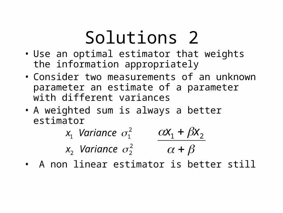
Solutions 2• Use an optimal estimator that weights the

information appropriately• Consider two measurements of an unknown

parameter an estimate of a parameter with different variances

• A weighted sum is always a better estimator

• A non linear estimator is better still

222

211

Variancex

Variancex

21 xx

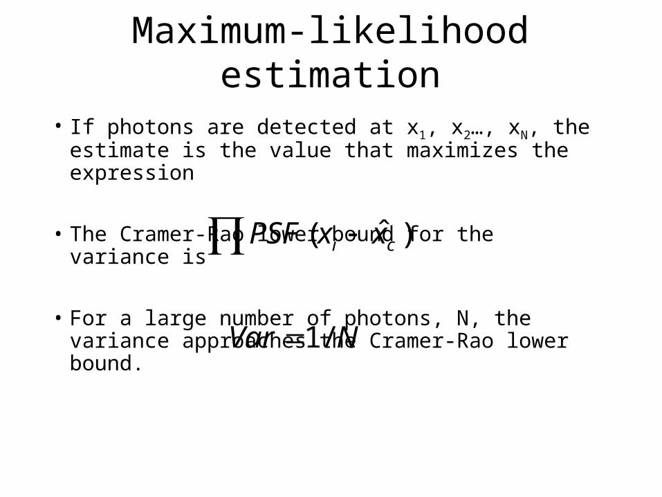
Maximum-likelihood estimation

• If photons are detected at x1, x2…, xN, the estimate is the value that maximizes the expression

• The Cramer-Rao lower bound for the variance is

• For a large number of photons, N, the variance approaches the Cramer-Rao lower bound.

)ˆ( ci xxPSF

NVar /1

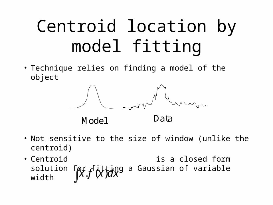
• Technique relies on finding a model of the object

• Not sensitive to the size of window (unlike the centroid)

• Centroid is a closed form solution for fitting a Gaussian of variable width

Centroid location by model fitting

Model Data

dxxfx )(.

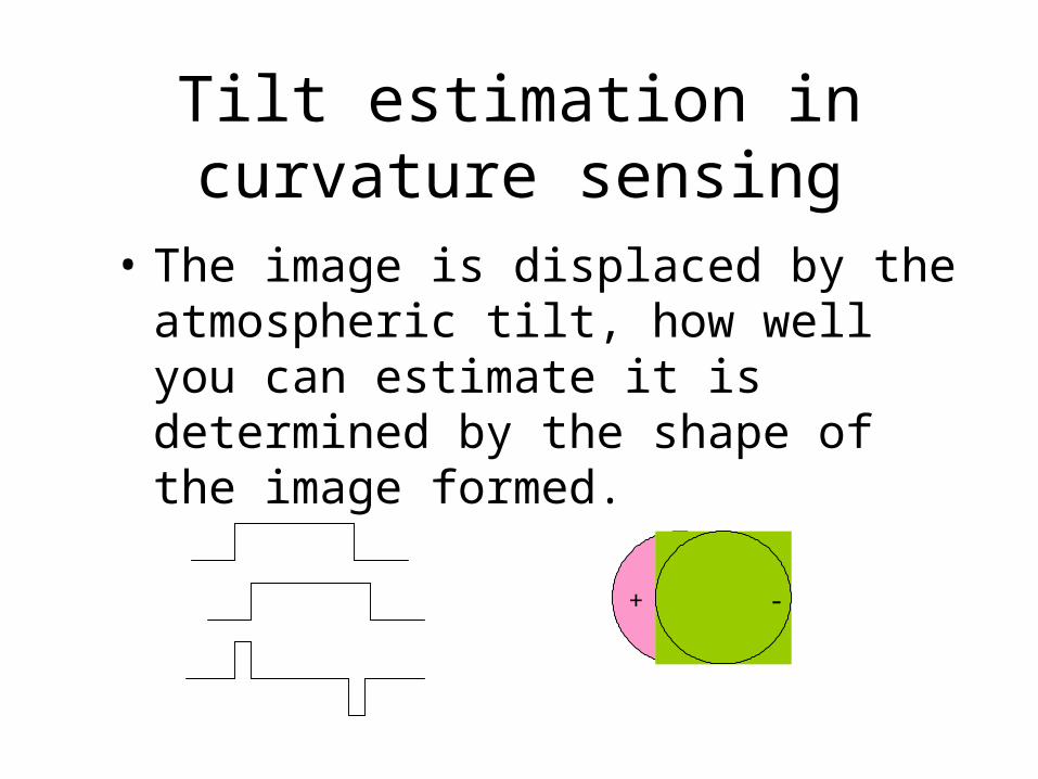
Tilt estimation in curvature sensing

• The image is displaced by the atmospheric tilt, how well you can estimate it is determined by the shape of the image formed.

+ -

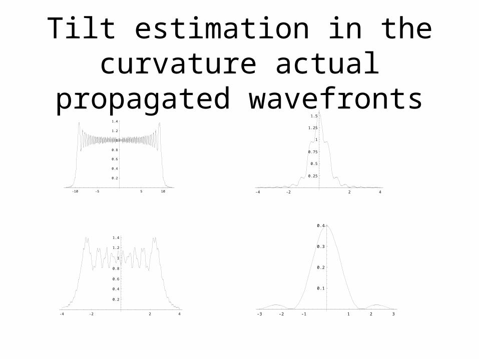
Tilt estimation in the curvature actual propagated wavefronts

-10 -5 5 10

0.2

0.4

0.6

0.8

1

1.2

1.4

-4 -2 2 4

0.2

0.4

0.6

0.8

1

1.2

1.4

-4 -2 2 4

0.25

0.5

0.75

1

1.25

1.5

-3 -2 -1 1 2 3

0.1

0.2

0.3

0.4

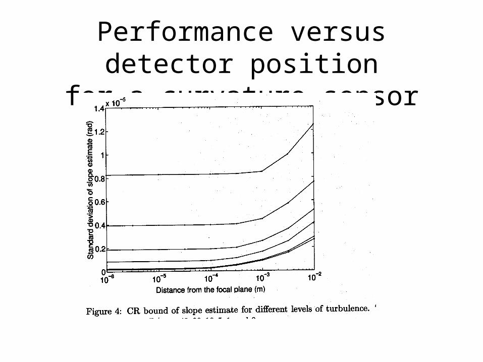
Performance versus detector positionfor a curvature sensor

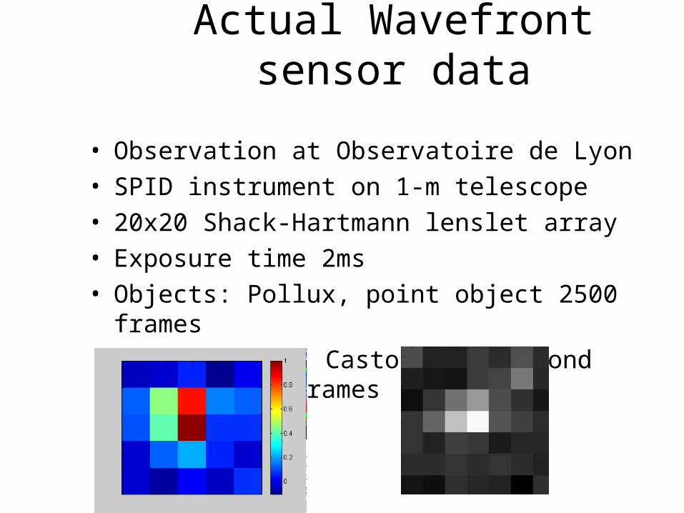
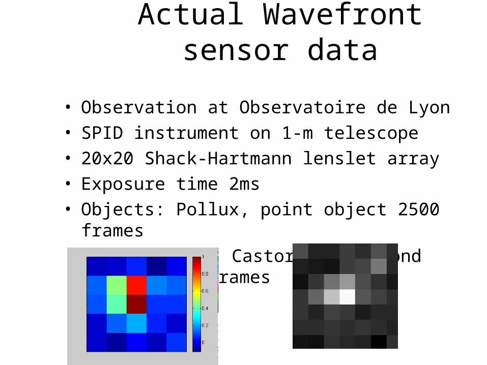
Actual Wavefront sensor data

• Observation at Observatoire de Lyon

• SPID instrument on 1-m telescope

• 20x20 Shack-Hartmann lenslet array

• Exposure time 2ms

• Objects: Pollux, point object 2500 frames

Castor3 arc second binary 2500 frames

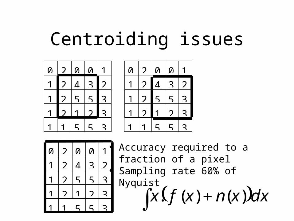
Centroiding issues

5 3 5 2 1

2 3 1 2 1

3 2 4 2 1

0 1 0 2 0

5 3 5 1 1

5 3 5 2 1

2 3 1 2 1

3 2 4 2 1

0 1 0 2 0

5 3 5 1 1

5 3 5 2 1

2 3 1 2 1

3 2 4 2 1

0 1 0 2 0

5 3 5 1 1

• Accuracy required to a fraction of a pixel

• Sampling rate 60% of Nyquist

dxxnxfx )()(.

• Need a good model of the object

• In each lenslet of the Shack-Hartmann acts like a small telescope the dominant effect is one of tilt.

=> We have a large number of images of the same object shifted before they are sampled.

Finding the model

Solution: approach

• Use blind deconvolution to find model• MAP framework (Hardie et al, FLIR)• Data-capturing process:

• Choose initially so that

• Prior information:– Laplacian smoothness for the optics

– Maximum entropy for CCD

noise CCD} optics fsubsample{ data

δ f noise CCD} opticssubsample{ data

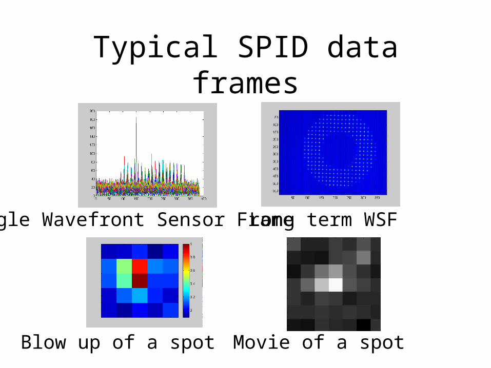
Typical SPID data frames

Single Wavefront Sensor Frame Long term WSF

Blow up of a spot Movie of a spot

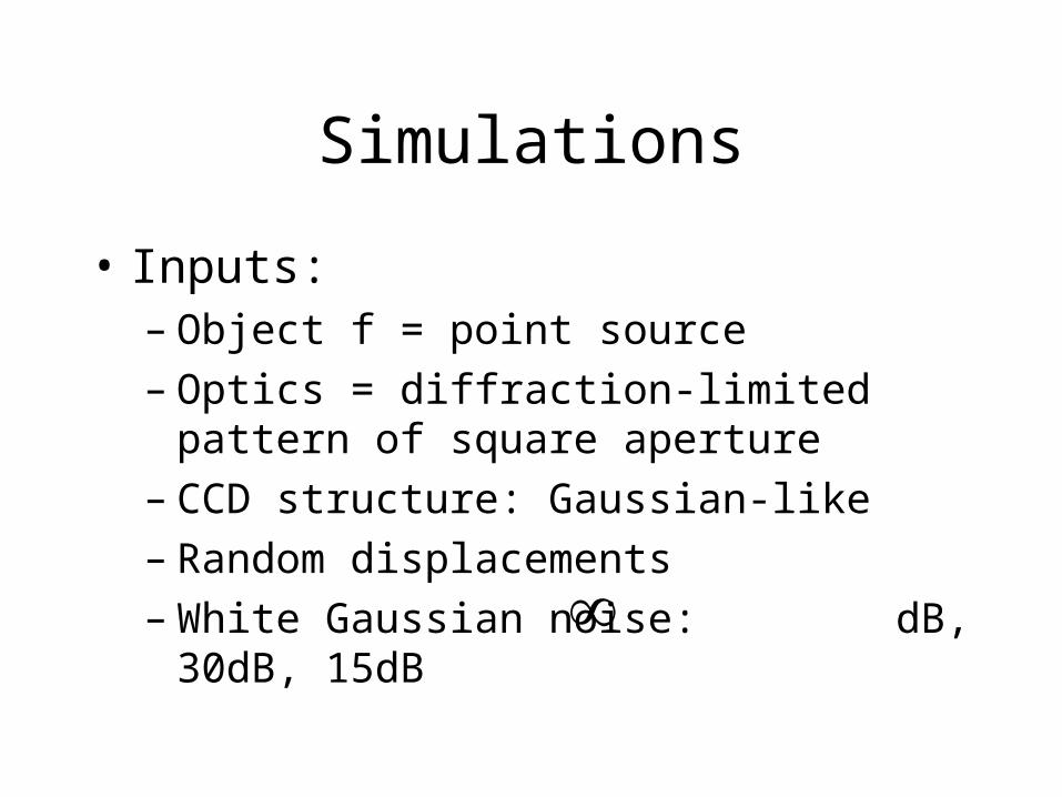
Simulations

• Inputs:– Object f = point source– Optics = diffraction-limited pattern of square

aperture– CCD structure: Gaussian-like– Random displacements– White Gaussian noise: dB, 30dB, 15dB

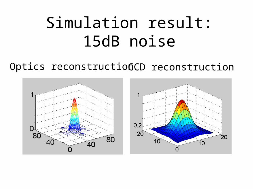
Simulation result: 15dB noise

Optics reconstruction CCD reconstruction

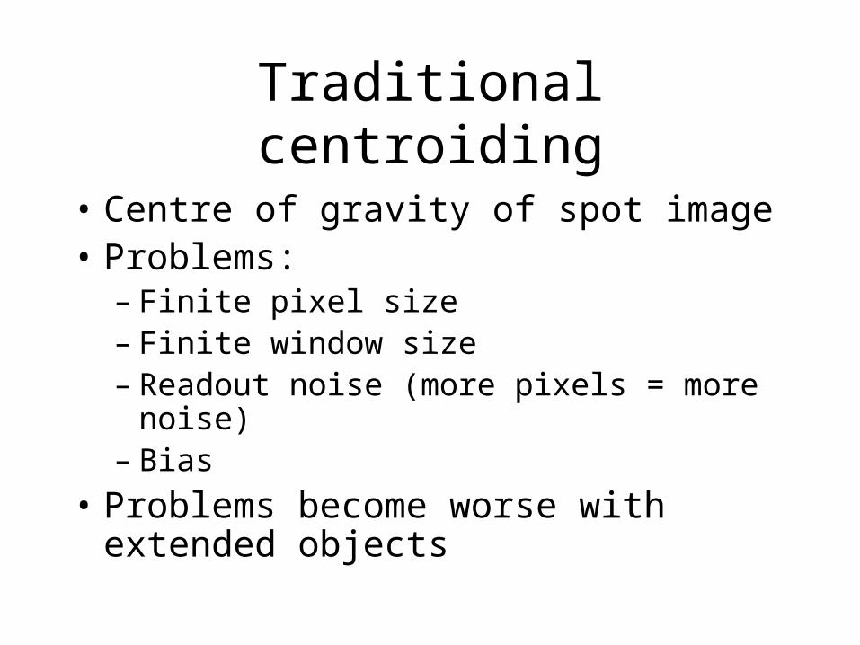
Traditional centroiding

• Centre of gravity of spot image• Problems:

– Finite pixel size– Finite window size– Readout noise (more pixels = more noise)– Bias

• Problems become worse with extended objects

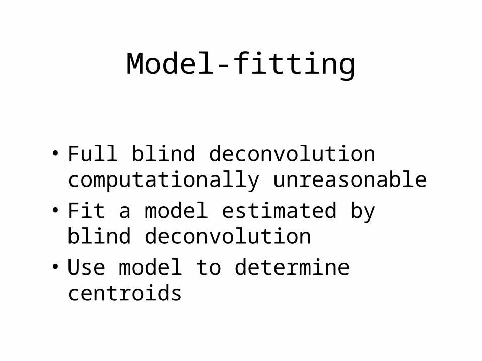
Model-fitting

• Full blind deconvolution computationally unreasonable

• Fit a model estimated by blind deconvolution

• Use model to determine centroids

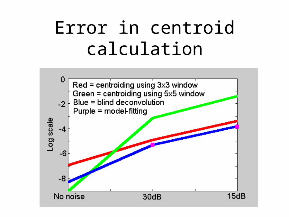
Error in centroid calculation

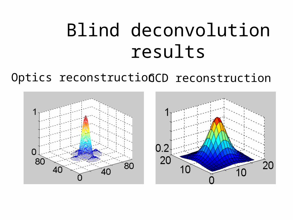
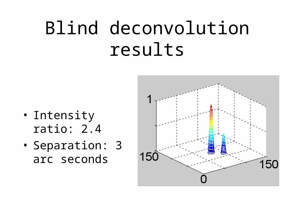
Blind deconvolution results

Optics reconstruction CCD reconstruction

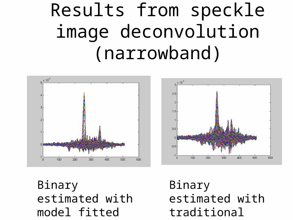
Results from speckle image deconvolution (narrowband)

Binary estimated with model fitted centroids

Binary estimated with traditionalcentroids

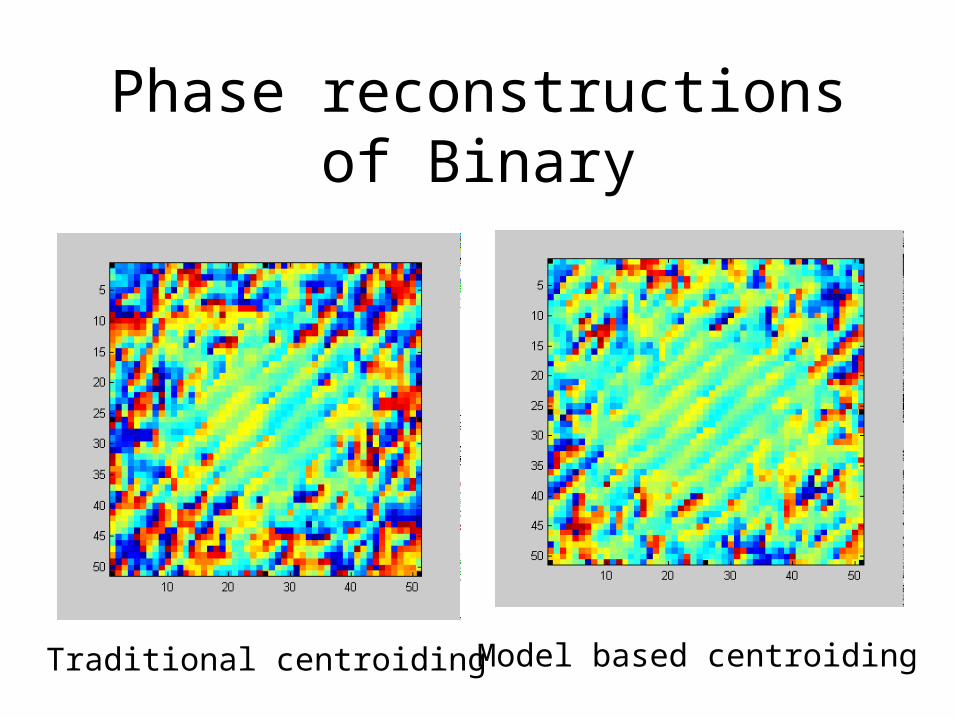
Phase reconstructions of Binary

Traditional centroiding Model based centroiding

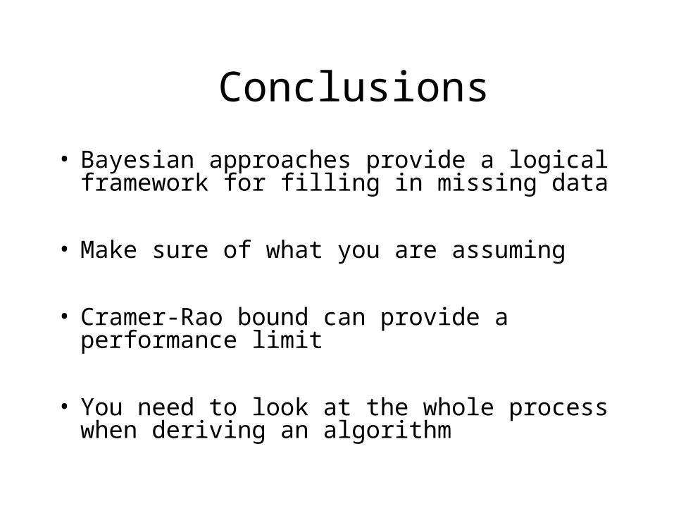
Conclusions

• Bayesian approaches provide a logical framework for filling in missing data

• Make sure of what you are assuming

• Cramer-Rao bound can provide a performance limit

• You need to look at the whole process when deriving an algorithm

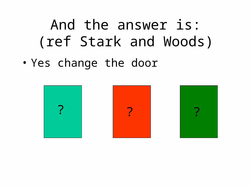
And the answer is:(ref Stark and Woods)

• Yes change the door

? ??

Actual Wavefront sensor data

• Observation at Observatoire de Lyon

• SPID instrument on 1-m telescope

• 20x20 Shack-Hartmann lenslet array

• Exposure time 2ms

• Objects: Pollux, point object 2500 frames

Castor3 arc second binary 2500 frames

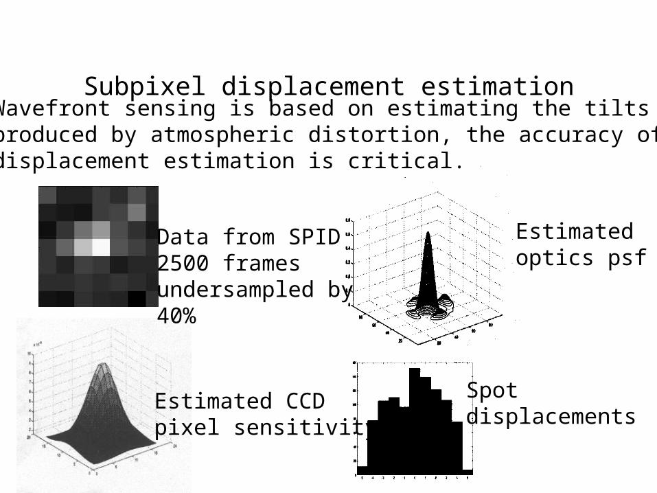
Subpixel displacement estimationWavefront sensing is based on estimating the tilts produced by atmospheric distortion, the accuracy ofdisplacement estimation is critical.

Data from SPID2500 framesundersampled by40%

Estimated CCD pixel sensitivity

Estimatedoptics psf

Spot displacements

Explanation of the terms

• Results from

Possible phase functionsZernike basis

The inverse problem

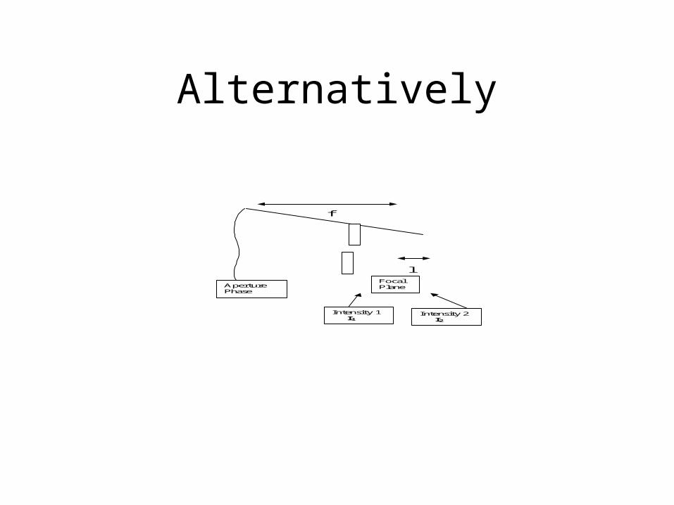
Alternatively

Focal Plane Aperture

Phase

Intensity 1 I1

Intensity 2 I2

l

f

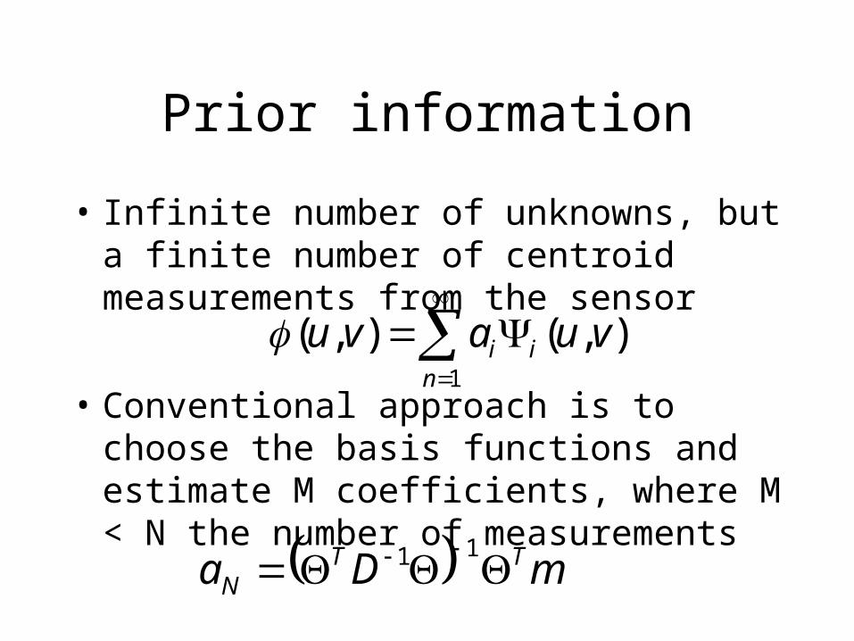
Prior information

• Infinite number of unknowns, but a finite number of centroid measurements from the sensor

• Conventional approach is to choose the basis functions and estimate M coefficients, where M < N the number of measurements

1

),(),(n

ii vuavu

mDa TTN

11

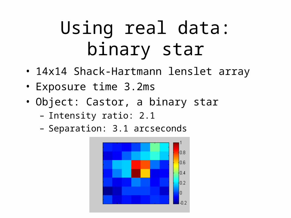
Using real data: binary star

• 14x14 Shack-Hartmann lenslet array

• Exposure time 3.2ms

• Object: Castor, a binary star– Intensity ratio: 2.1

– Separation: 3.1 arcseconds

Blind deconvolution results

• Intensity ratio: 2.4• Separation: 3 arc

seconds