Embed Size (px)
Citation preview

Wavefront Sensing I
Richard Lane
Department of Electrical and Computer Engineering
University of Canterbury
Christchurch
New Zealand

Location

Astronomical Imaging Grouppast and present
Dr Richard LaneProfessor Peter GoughAssociate Professor P. J. BonesAssociate Professor Peter CottrellProfessor Richard Bates
Dr Bonnie Law Dr Roy Irwan Dr Rachel Johnston Dr Marcos van DamDr Valerie Leung Richard ClareYong Chew Judy Mohr

Contents
• Session 1 – Principles
• Session 2 – Performances
• Session 3 – Wavefront Reconstruction for 3D

Principles of wavefront sensing
• Introduction
• Closed against open loop wavefront sensing
• Nonlinear wavefront sensing
• Shack-Hartmann
• Curvature
• Geometric
• Conclusions

Imaging a star

The effect of turbulence

Adaptive Optics system
Wavefrontsensor
Image plane
Deformablemirror
Distorted incomingwavefront
telescope

Closed loop system
K Compensation system
error
Noise
True output
Measured output
Desired Output (zero phase)
Reduces the effects of disturbances such as telescope vibration, modelling errors by the loop gain
Does not inherently improve the noise performanceunless the closed loop measurements are easier to make
Design limited by stability constraints
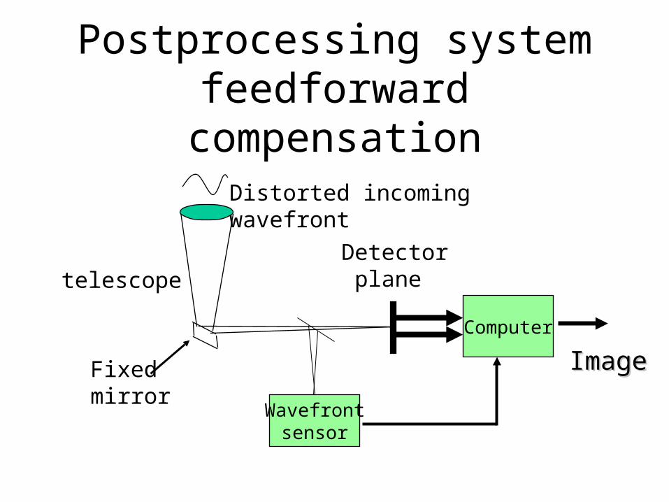
Postprocessing systemfeedforward compensation
Wavefrontsensor
Detector plane
Distorted incomingwavefront
telescope
Fixedmirror
Computer
ImageImage

Open loop system (SPID)
Distortion estimation
Estimatedoutput
True image
Wavefront sensor
Compensation Distortion by the atmosphere
Sensitive to modelling errors
No stability issues with computer post processing
Problem is not noise but errors in modelling the system
timeTemporal coherenceof the atmosphere
T

Modelling the problem (step1)
• The relationship between the measured data and the object and the point spread function is linear
Data object convolution point spread function noise
(psf)• A linear relationship would mean that if we multiply
the input by α we multiply the output by α. The output doesn’t change form
),(),(),(),( yxnyxhyxfyxd
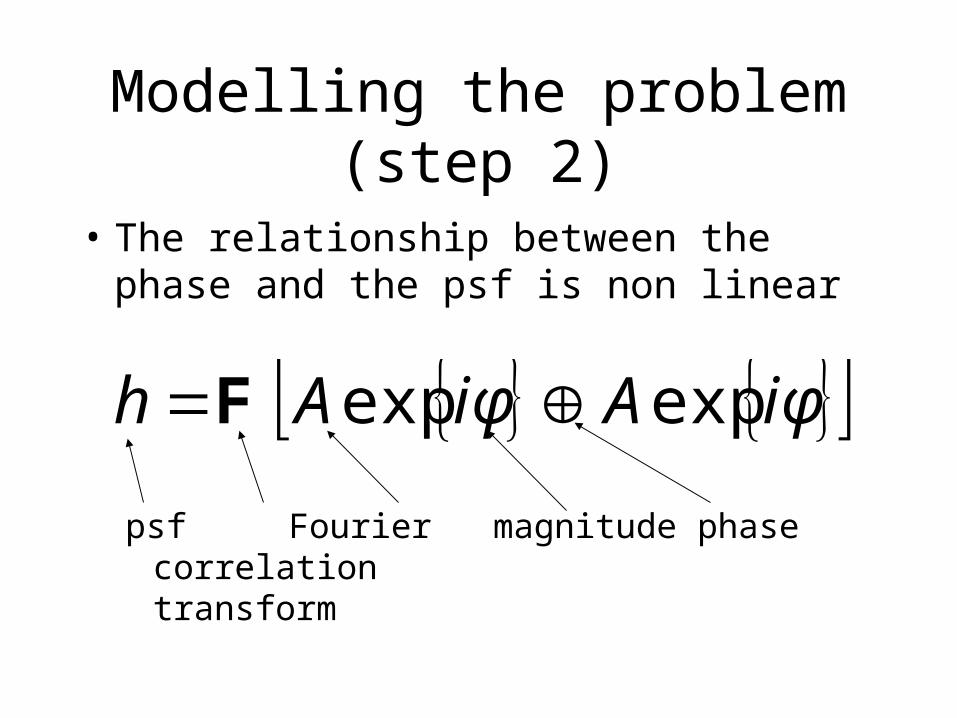
Modelling the problem (step 2)
• The relationship between the phase and the psf is non linear
psf Fourier magnitude phase correlation transform
iφAiφA h expexp F

Correct MAP estimate Wrapped ambiguity
ML estimation MAP estimation
Phase retrieval
• Nonlinearity caused by 2 wrapping interacting with smoothing

Role of typical wavefront sensor
• To produce a linear relationship between the measurements and the phase– Speeds up reconstruction– Guarantees a solution– Degrades the ultimate performance
phase weighting basis function
1
),(),(n
ii vuavu

Solution is by linear equations
Measurement Interaction Basis functionvector matrix Coefficents• ith column of Θ corresponds to the measurement that would
occur if the phase was the ith basis function• Three main issues
– What has been lost in linearising?– How well you can solve the system of equations?– Is it the right equations?
am
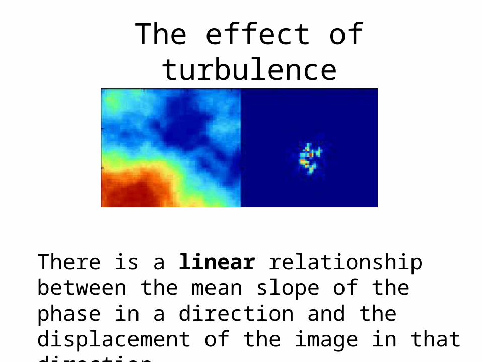
The effect of turbulence
There is a linear relationship between the mean slope of the phase in a direction and the displacement of the image in that direction.
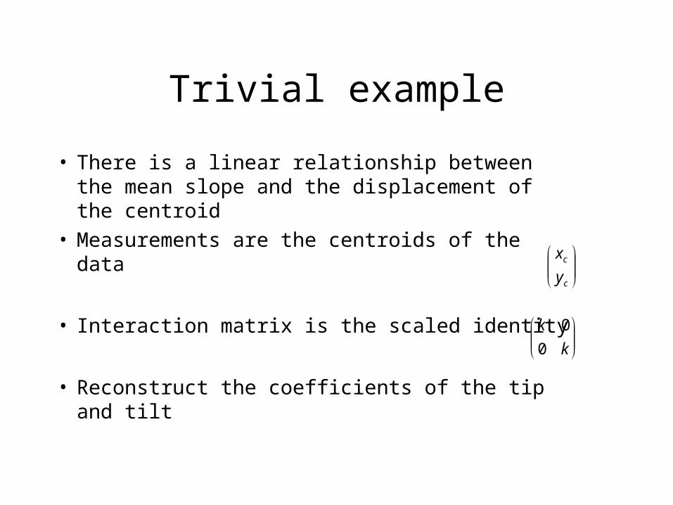
Trivial example
• There is a linear relationship between the mean slope and the displacement of the centroid
• Measurements are the centroids of the data
• Interaction matrix is the scaled identity
• Reconstruct the coefficients of the tip and tilt
c
c
y
x
k
k
0
0

Quality of the reconstruction• The centroid proportional to the mean slope
(Primot el al, Welsh et al). • The best Strehl requires estimating the least mean
square (LMS) phase (Glindemann).
• To distinguish the mean and LMS slope you need to estimate the coma and higher order terms
Mean slope
LMS slope
Phase
50 100 150 200 250
50
100
150
200
250
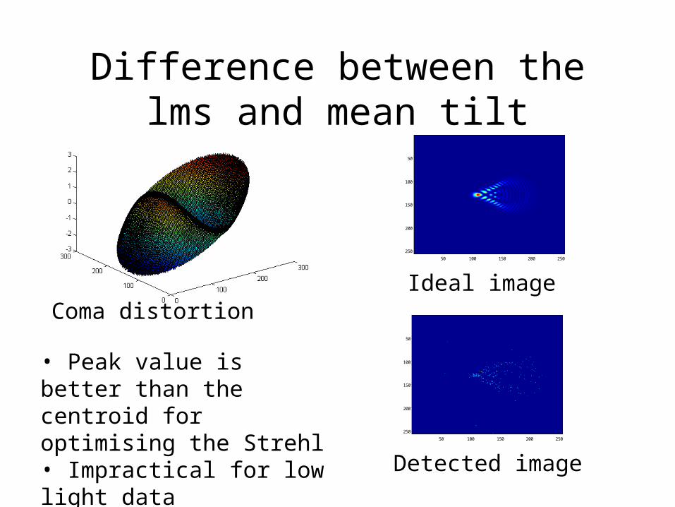
Coma distortion
Detected image
• Peak value is better than the centroid for optimising the Strehl• Impractical for low light data 50 100 150 200 250
50
100
150
200
250
Difference between the lms and mean tilt
Ideal image

Where to from here
• The real problem is how to estimate higher aberration orders.
• Wavefront sensor can be divided into:– pupil plane techniques, that measure slopes
(curvatures) in the divided pupil plane, • Shack-Hartmann• Curvature (Roddier), Pyramid (Ragazonni)• Lateral Shearing Interferometers
– Image plane techniques that go directly from data in the image plane to the phase (nonlinear)
• Phase diversity (Paxman)• Phase retrieval

Geometric wavefront sensing
• Pyramid, Shack-Hartmann and Curvature sensors are all essentially geometric wavefront sensors
• Rely on the fact that light propagates perpindicularly to the wavefront.
• A linear relationship between the displacement and the slope
• Essentially achromatic
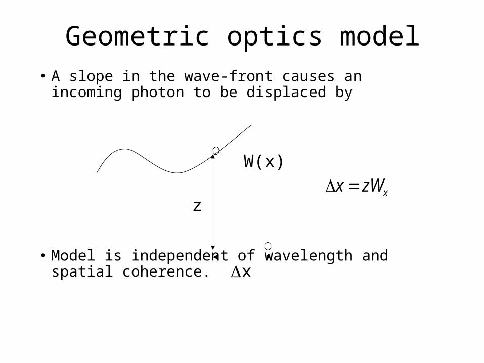
Geometric optics model• A slope in the wave-front causes an incoming photon
to be displaced by
• Model is independent of wavelength and spatial coherence.
z
W(x)
x
xzWx

Generalized wave-front sensor• This is the basis of the two most common
wave-front sensors.
Converging lens
Aberration
Focal plane
Curvature sensor
Shack-Hartmann

Trade-off
• For fixed photon count, you trade off the number of modes you can estimate in the phase screen against the accuracy with which you can estimate them
• To estimate a high number of modes you need good resolution in the pupil plane
• To make the estimate accurately you need good resolution in the image plane

Properties of a wave-front sensor
• Linearization: want a linear relationship between the wave-front and the measurements.
• Localization: the measurements must relate to a region of the aperture.
• Broadband: the sensor should operate over a wide range of wavelengths.
Geometric Optics regime
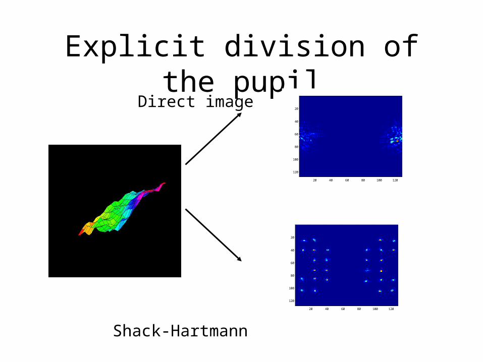
Explicit division of the pupilDirect image
Shack-Hartmann
20 40 60 80 100 120
20
40
60
80
100
120
20 40 60 80 100 120
20
40
60
80
100
120

Shack-Hartmann sensor
0
5
10
15
20
0
5
10
15
20-10
0
10
20
05
1015
20
0
5
10
15
200
0.02
0.04
0.06
0.08
• Subdivide the aperture and converge each subdivision to a different point on the focal plane.
• A wave-front slope, Wx, causes a displacement of each image by zWx.

Fundamental problem• Resolution in the pupil plane is inversely
proportional to the resolution in the image plane
• You can have good resolution in one but not both (Uncertainty principle)
D
w
Pupil
Image
wD
1

Loss of information due to subdivision
• Cannot measure the average phase difference between the apertures
• Can only determine the mean phase slope within an aperture
• As the apertures become smaller the light per aperture drops
• As the aperture size drops below r0 (Fried parameter) the spot centroid becomes harder to measure

• Subdivided aperture
5 6 7 8 9 100
0.01
0.02
0.03
0.04
0.05
0.06
Log10
Number of photons
Mea
n sq
uare
d-er
ror D/r
0=1
D/r0=2
D/r0=4

Implicit subdivision
• If you don’t image in the focal plane then the image looks like a blurred version of the aperture
• If it looks like the aperture then you can localise in the aperture
Focal plane
Aperture
Defocused Aperture I1
Defocused Aperture I2
l
lffz
)(

Explanation of the underlying principle
• If there is a deviation from the average curvature in the wavefront then on one side the image will be brighter than the other
Focal Plane Aperture
Phase
Intensity 1 I1
Intensity 2 I2
l
f
If there is no curvaturefrom the atmosphere thenit is equally bright on bothsides of focus.

Slope based analysis of the curvature sensor
Planar Wavefront
Detector Pixels
Distorted Wavefront
Detector Pixels
The displacement of light from one pixel to its neighbour iss determined by the slope of the wavefront

Slope based analysis of the curvature sensor
Distorted Wavefront
Detector Pixels
Distorted Wavefront
Detector Pixels
•The signal is the difference between two slope signals→Curvature
Distorted Wavefront
Detector Pixels

Phase information localisation in the curvature sensor
r0?
Kolmogorov phase screen
Detector Plane
Blurring due to the roughness of the phase screen
Focal plane
Aperture resolution
Detector plane blurring
• Diffraction blurring + geometric expansion

• Localization comes from the short effective propagation distance,
• Linear relationship between the curvature in the aperture and the normalized intensity difference:
• Broadband light helps reduce diffraction effects.
Curvature sensing
A p e r t u r e
D e f o c u s e d i m a g e I 1
D e f o c u s e d i m a g e I 2
l
f l
lffz
)(

Curvature sensing signal
Simulated intensity measurement
Curvature sensing estimate
• The intensity signal gives an approximate estimate of the curvature.
• Two planes help remove scintillation effects

Irradiance transport equation
WIWIz
I 2.
I
IWzWz
II
II
.2
12
12
• Linear approximation gives
WzIWIzI 21 .
WzIWIzI 22 .

Solution inside the boundary
)(21
21yyxx WWz
II
II
• There is a linear relationship between the signal and the curvature.
• The sensor is more sensitive for large effective propagation distances.
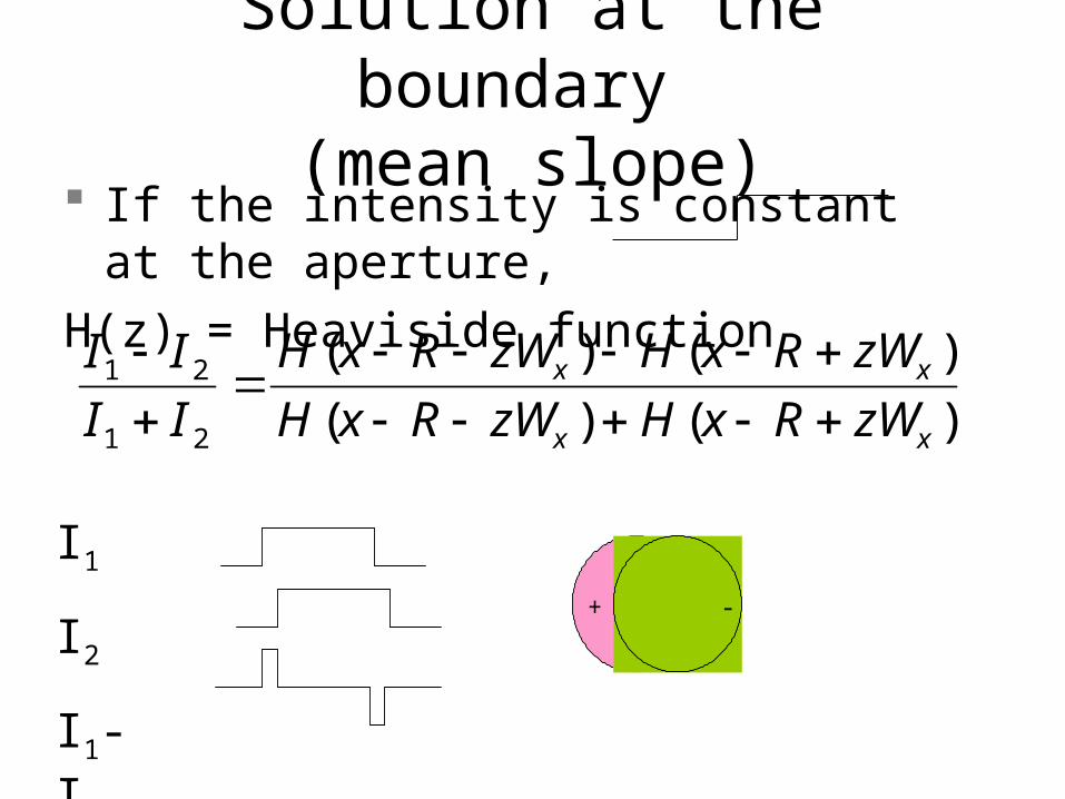
Solution at the boundary (mean slope)
)()(
)()(
21
21
xx
xx
zWRxHzWRxH
zWRxHzWRxH
II
II
If the intensity is constant at the aperture,
H(z) = Heaviside function
+ -
I1
I2
I1- I2

The wavefront also changes
222
22
2
22 )(
816)(
2
11 I
II
IWWz
• As the wave propagates, the wave-front changes according to:
• As the measurement approaches the focal plane the distortion of the wavefront becomes more important, and needs to be incorpoarated (van Dam and Lane)

Non-linearity due to the wavefront changing
• As a consequence the intensity also changes!
• So, to second order :
• The sensor is non-linear!
)(1
)(2
21
21
TKz
WWz
II
II yyxx

Origin of terms
• Due to the difference in the curvature in the x- and y- directions (astigmatism).
• Due to the local wave-front
slope, displacing the curvature
measurement.
2xyyyxx WWWK
yyyyxxyyxyyxxxxx WWWWWWWWT
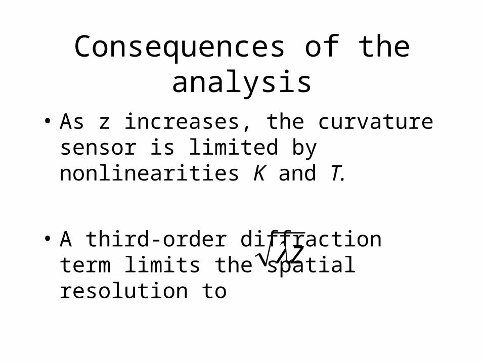
Consequences of the analysis
• As z increases, the curvature sensor is limited by nonlinearities K and T.
• A third-order diffraction term limits the spatial resolution to
z

Analysis of the curvature sensor
As the propagation distance, z, increases,
• Sensitivity increases.
• Spatial resolution decreases.
• The relationship between the signal and the curvature becomes non-linear.
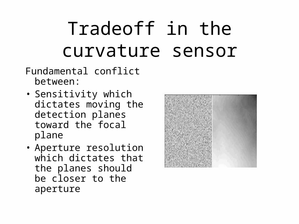
Tradeoff in the curvature sensor
Fundamental conflict between:
• Sensitivity which dictates moving the detection planes toward the focal plane
• Aperture resolution which dictates that the planes should be closer to the aperture

• Slopes in the wave-front causes the intensity distribution to be stretched like a rubber sheet
• Wavefront sensing maps the distribution backto uniform
Geometric optics model
z
W(x)
xxzWx
20 40 60 80 100 120
20
40
60
80
100
120

• The intensity can be viewed as a probability density function (PDF) for photon arrival.
• As the wave propagates, the PDF evolves.
• The cumulative distribution function (CDF) also changes.
Intensity distribution as a PDF
Intensity distribution
Photon arrival p(x)
x

• Take two propagated images of the aperture.
D=1 m, r0=0.1 m and λ=589 nm.
Intensity at -z
Intensity at z

• Can prove using the irradiance transport equation and the wave-front transport equation that
• This relationship is exact for geometric optics, even when there is scintillation.
• Can be thought of as the light intensity being a rubber sheet being stretched unevenly
),(CDF),(CDF)0,(CDF zx
Wzxz
x
Wzxx

• Use the cumulative distribution function to match points in the two intensity distributions.
• The slope is given by
x1 x2
z
xxxxW
x 2
21
2
21

Results in one dimensionActual (black) and reconstructed (red) derivative
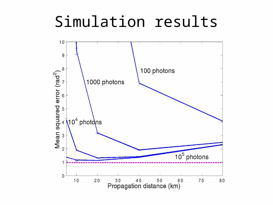
Simulation results

Comparison with Shack-Hartmann

Conclusions
• Fundamentally geometric wavefront sensors are all based on the same linear relationship between slope and displaced light
• All sensors trade off the number of modes you can estimate against the quality of the estimate
• The main difference between the curvature and Shack-Hartmann is how they divide the aperture
• Question is how to make this tradeoff optimally.