Embed Size (px)
Citation preview
Wave scattering by an integral stiffener
by
Ricky Steven Reusser
A thesis submitted to the graduate faculty
in partial fulfillment of the requirements for the degree of
MASTER OF SCIENCE
Major: Engineering Mechanics
Program of Study Committee:
Stephen D. Holland, Major Professor
Dale E. Chimenti
Ron A. Roberts
Thomas J. Rudolphi
Iowa State University
Ames, Iowa
2012
Copyright c© Ricky Steven Reusser, 2012. All rights reserved.
ii
TABLE OF CONTENTS
LIST OF FIGURES . . . . . . . . . . . . . . . . . . . . . . . . . . . . . . . . . . . iv
ACKNOWLEDGEMENTS . . . . . . . . . . . . . . . . . . . . . . . . . . . . . . . vii
ABSTRACT . . . . . . . . . . . . . . . . . . . . . . . . . . . . . . . . . . . . . . . . viii
CHAPTER 1. Introduction . . . . . . . . . . . . . . . . . . . . . . . . . . . . . . 1
CHAPTER 2. Guided plate wave scattering at vertical stiffeners and its
effect on source location . . . . . . . . . . . . . . . . . . . . . . . . . . . . . . . 2
2.1 Abstract . . . . . . . . . . . . . . . . . . . . . . . . . . . . . . . . . . . . . . . . 2
2.2 Introduction . . . . . . . . . . . . . . . . . . . . . . . . . . . . . . . . . . . . . . 3
2.2.1 Spacecraft Leak Location . . . . . . . . . . . . . . . . . . . . . . . . . . 4
2.3 Transmission across a Stiffener . . . . . . . . . . . . . . . . . . . . . . . . . . . 5
2.3.1 Theory . . . . . . . . . . . . . . . . . . . . . . . . . . . . . . . . . . . . 6
2.3.2 Experiment . . . . . . . . . . . . . . . . . . . . . . . . . . . . . . . . . . 6
2.3.3 Comparison of Experiment with BEM Simulation . . . . . . . . . . . . . 11
2.4 Spacecraft Leak Location . . . . . . . . . . . . . . . . . . . . . . . . . . . . . . 14
2.4.1 Theory . . . . . . . . . . . . . . . . . . . . . . . . . . . . . . . . . . . . 15
2.4.2 An Algorithm for Selecting a Frequency Band . . . . . . . . . . . . . . . 16
2.4.3 Experimental Configuration . . . . . . . . . . . . . . . . . . . . . . . . . 17
2.5 Summary and conclusions . . . . . . . . . . . . . . . . . . . . . . . . . . . . . . 22
Bibliography . . . . . . . . . . . . . . . . . . . . . . . . . . . . . . . . . . . . . . . . 23
CHAPTER 3. Reflection and transmission of guided plate waves by vertical
stiffeners . . . . . . . . . . . . . . . . . . . . . . . . . . . . . . . . . . . . . . . . 27
3.1 Abstract . . . . . . . . . . . . . . . . . . . . . . . . . . . . . . . . . . . . . . . . 27

iii
3.2 Introduction . . . . . . . . . . . . . . . . . . . . . . . . . . . . . . . . . . . . . . 28
3.3 Approximate Model . . . . . . . . . . . . . . . . . . . . . . . . . . . . . . . . . 30
3.3.1 High aspect ratio approxmation . . . . . . . . . . . . . . . . . . . . . . . 30
3.3.2 Small junction approximation . . . . . . . . . . . . . . . . . . . . . . . . 30
3.3.3 Low frequency approximation . . . . . . . . . . . . . . . . . . . . . . . . 31
3.3.4 Generalized Impedance . . . . . . . . . . . . . . . . . . . . . . . . . . . 32
3.3.5 Junction . . . . . . . . . . . . . . . . . . . . . . . . . . . . . . . . . . . . 32
3.3.6 Force Balance . . . . . . . . . . . . . . . . . . . . . . . . . . . . . . . . . 34
3.3.7 Plate waves . . . . . . . . . . . . . . . . . . . . . . . . . . . . . . . . . . 35
3.4 Calculation of Generalized Impedance . . . . . . . . . . . . . . . . . . . . . . . 39
3.4.1 Characteristic Impedance of Plate Waves . . . . . . . . . . . . . . . . . 39
3.4.2 Stiffener Impedance . . . . . . . . . . . . . . . . . . . . . . . . . . . . . 41
3.5 Results . . . . . . . . . . . . . . . . . . . . . . . . . . . . . . . . . . . . . . . . . 46
3.5.1 S0 Transmission . . . . . . . . . . . . . . . . . . . . . . . . . . . . . . . 47
3.5.2 A0 Transmission . . . . . . . . . . . . . . . . . . . . . . . . . . . . . . . 50
3.5.3 Conclusion . . . . . . . . . . . . . . . . . . . . . . . . . . . . . . . . . . 51
Bibliography . . . . . . . . . . . . . . . . . . . . . . . . . . . . . . . . . . . . . . . . 54
CHAPTER 4. Conclusions . . . . . . . . . . . . . . . . . . . . . . . . . . . . . . . 56
4.1 Summary . . . . . . . . . . . . . . . . . . . . . . . . . . . . . . . . . . . . . . . 56
4.2 Recommendations for future research . . . . . . . . . . . . . . . . . . . . . . . . 57
APPENDIX A. APPROXIMATE GUIDED WAVE THEORY . . . . . . . . . 58

iv
LIST OF FIGURES
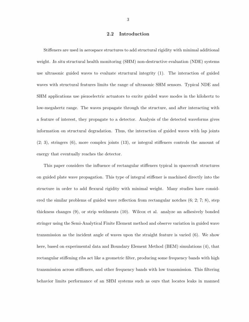
Figure 2.1 Photo of 6×6-foot sample showing experimental area isolated by butyl rubber
(seen as a low-reflection band on the perimeter). Source is marked with a
cross, and two sets of dots show the locations of laser vibrometer linear virtual-
array measurements of incident and scattered guided wave fields. Inset shows
stiffener cross-section with arrows representing waves incident upon as well as
transmitted and reflected by stiffener. . . . . . . . . . . . . . . . . . . . . 7
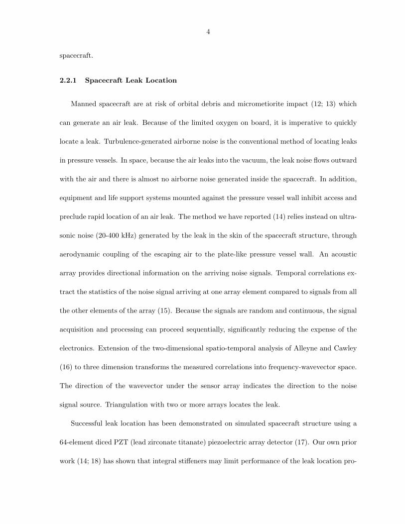
Figure 2.2 Measured normal component of particle velocity magnitude displayed as a
gray-scale plot in coordinate x and time t for the tall stiffener test section.
The wave amplitude is represented by the surface particle velocity vn . . . . 9
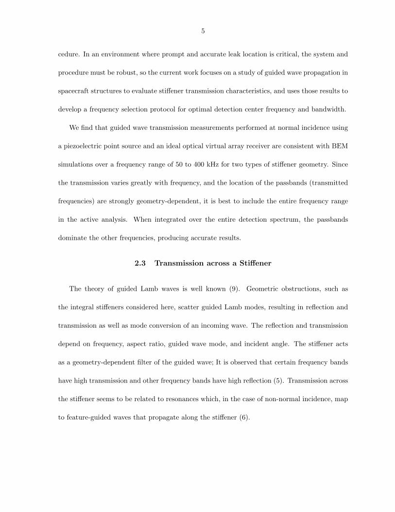
Figure 2.3 Measured dispersion curves for incident guided plate waves in the high aspect-
ratio test section. Calculate Lamb wave dispersion curves (dotted lines) are
superimposed. . . . . . . . . . . . . . . . . . . . . . . . . . . . . . . . . 10
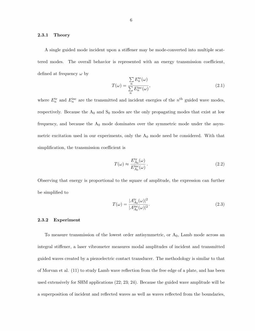
Figure 2.4 Experimental and theoretical energy transmission coefficients across the tall
aspect-ratio stiffener, with the incident guided wave at normal incidence to the
stiffener. The theoretical curve is the result of the boundary element method
calculation. . . . . . . . . . . . . . . . . . . . . . . . . . . . . . . . . . . 13
Figure 2.5 Experimental and theoretical energy transmission coefficients across the low
aspect ratio stiffener, with the incident guided wave at normal incidence to the
stiffener. The theoretical curve is the result of the boundary element method
calculation. . . . . . . . . . . . . . . . . . . . . . . . . . . . . . . . . . . 14
v
Figure 2.6 Leak location results for frequencies from 75-100 kHz. The “x” markings
show simulated leak locations, and the circle near the plate center shows the
detector array position. The diagonal dashed lines are the locations of the
integral stiffeners. . . . . . . . . . . . . . . . . . . . . . . . . . . . . . . . 19
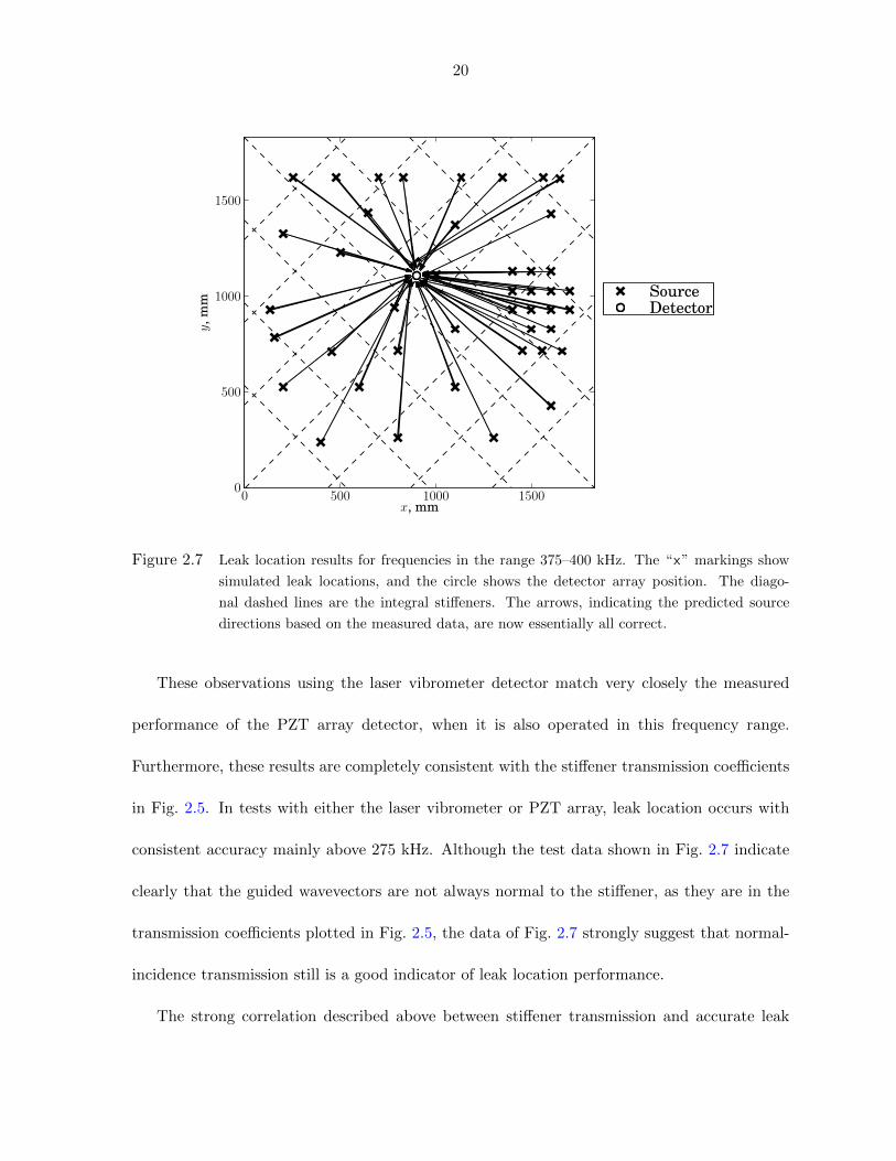
Figure 2.7 Leak location results for frequencies in the range 375–400 kHz. The “x” mark-
ings show simulated leak locations, and the circle shows the detector array
position. The diagonal dashed lines are the integral stiffeners. The arrows, in-
dicating the predicted source directions based on the measured data, are now
essentially all correct. . . . . . . . . . . . . . . . . . . . . . . . . . . . . . 20
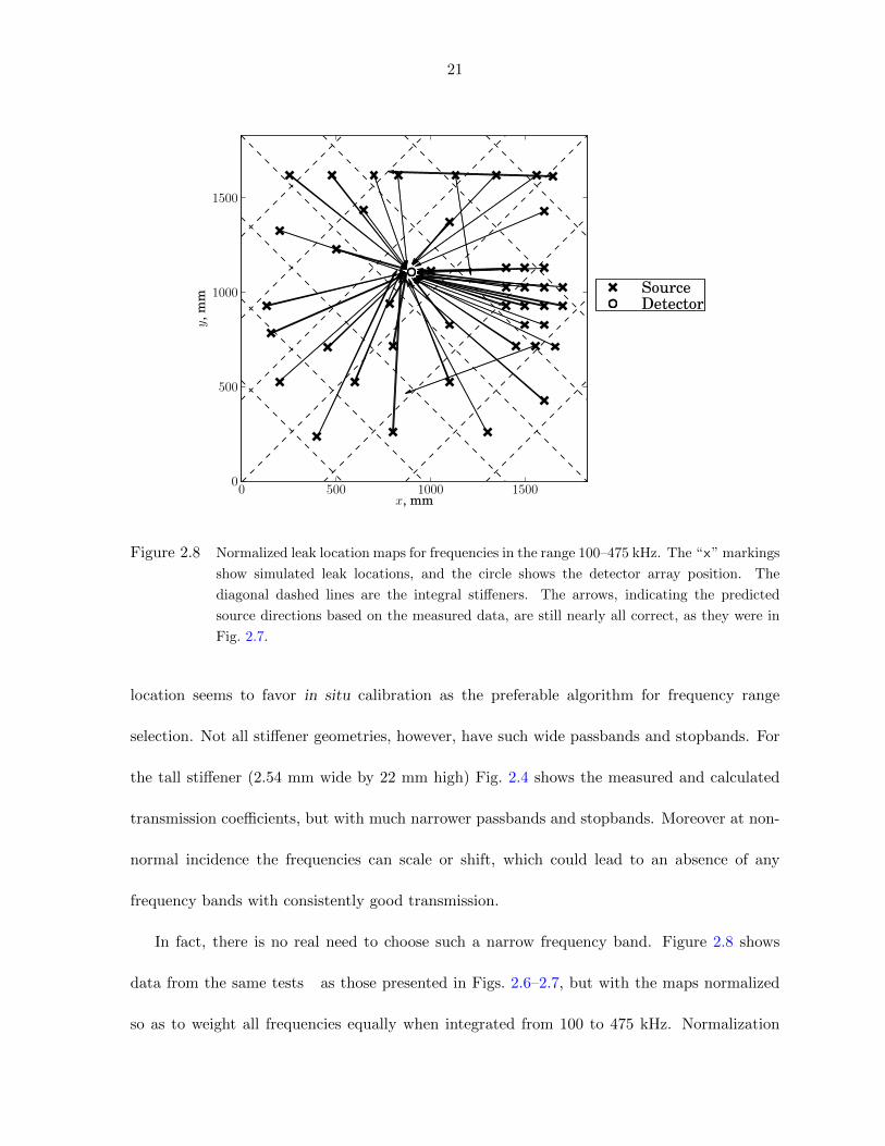
Figure 2.8 Normalized leak location maps for frequencies in the range 100–475 kHz. The
“x” markings show simulated leak locations, and the circle shows the detector
array position. The diagonal dashed lines are the integral stiffeners. The
arrows, indicating the predicted source directions based on the measured data,
are still nearly all correct, as they were in Fig. 2.7. . . . . . . . . . . . . . . 21
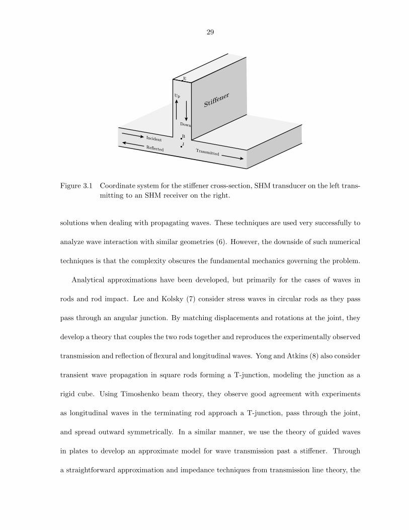
Figure 3.1 Coordinate system for the stiffener cross-section, SHM transducer on
the left transmitting to an SHM receiver on the right. . . . . . . . . . . 29
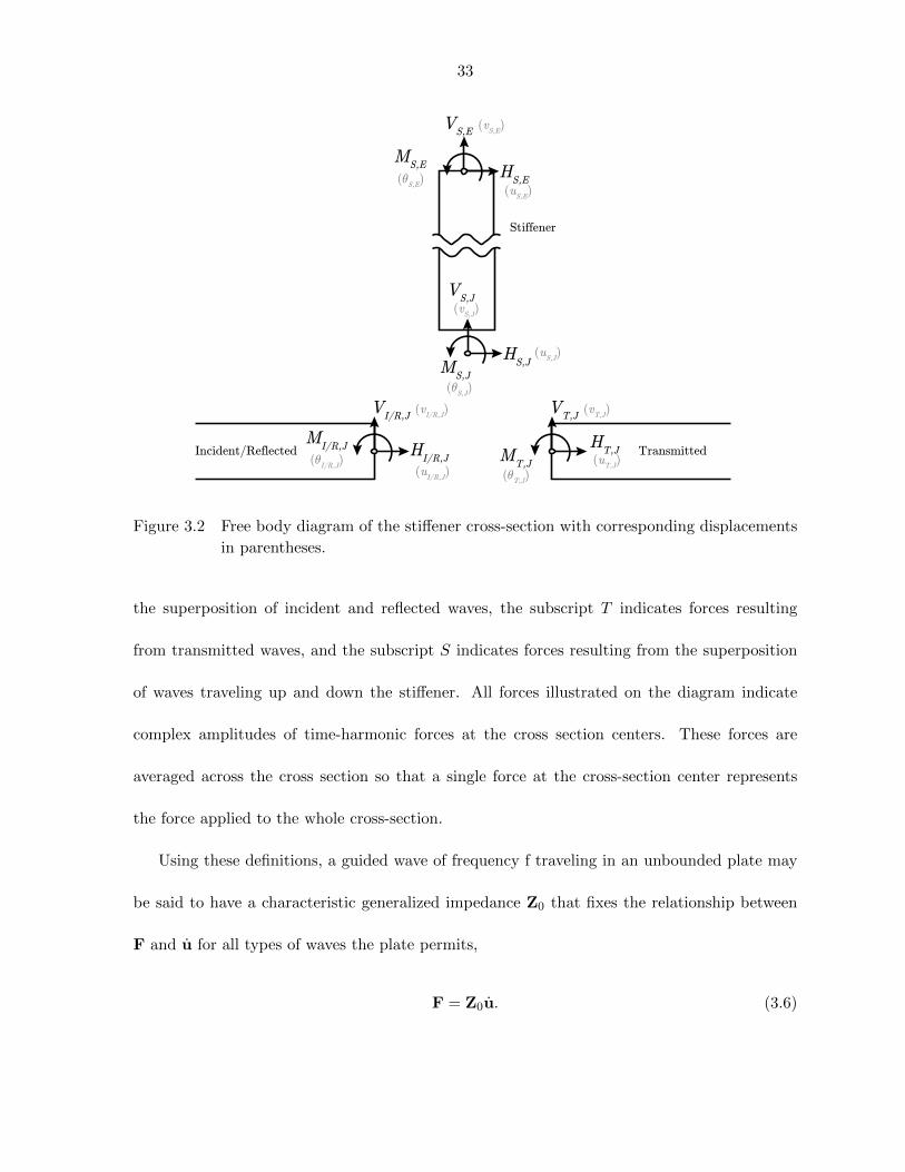
Figure 3.2 Free body diagram of the stiffener cross-section with corresponding dis-
placements in parentheses. . . . . . . . . . . . . . . . . . . . . . . . . . 33
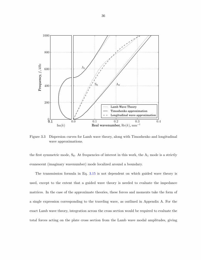
Figure 3.3 Dispersion curves for Lamb wave theory, along with Timoshenko and
longitudinal wave approximations. . . . . . . . . . . . . . . . . . . . . . 36
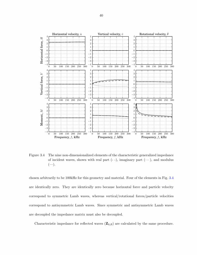
Figure 3.4 The nine non-dimensionalized elements of the characteristic generalized
impedance of incident waves, shown with real part (- -), imaginary part
(· · · ), and modulus (—). . . . . . . . . . . . . . . . . . . . . . . . . . . 40
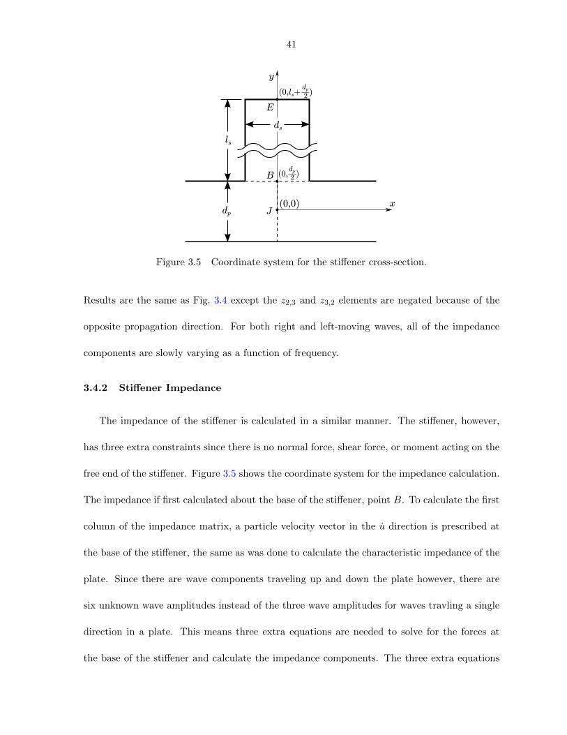
Figure 3.5 Coordinate system for the stiffener cross-section. . . . . . . . . . . . . 41
Figure 3.6 The nine non-dimensionalized elements of the stiffener impedance, ZS ,
shown with real part (- -), imaginary part (· · · ), and modulus (—). . . 46
Figure 3.7 S0 energy reflection and transmission coefficients for incident S0 Lamb
waves. Deformed shapes for lettered points plotted in Fig. 3.8. . . . . . 47

vi
Figure 3.8 Instantaneous deformed shapes for S0 Lamb waves incident from the left
at frequencies 50 kHz (a), 70 kHz (b), 95 kHz (c), 120 kHz (d), and 150
kHz (e). . . . . . . . . . . . . . . . . . . . . . . . . . . . . . . . . . . . 48
Figure 3.9 A0 energy reflection and transmission coefficients for incident A0 Lamb
waves. Deformed shapes for lettered points plotted in Fig. 3.11. . . . . 49
Figure 3.10 Comparison of A0 energy transmission coefficient with numerical solu-
tion and experimental data for incident A0 Lamb waves. . . . . . . . . 52
Figure 3.11 Instantaneous deformed shapes for A0 Lamb waves incident from the
left at frequencies 50 kHz (a), 75 kHz (b), 110 kHz (c), 125 kHz (d),
and 160 kHz (e). . . . . . . . . . . . . . . . . . . . . . . . . . . . . . . 53
A.1 A0 Energy transmission coefficient for incoming A0 waves using approx-
imate theory without wavenumber correction (top), with wavenumber
correction (middle), and with exact Lamb wave theory (bottom). . . . 65

vii
ACKNOWLEDGEMENTS
First and most importantly, I would like to thank my advisor, Dr. Steve Holland, for his
unending guidance and support in my graduate education. He has helped me through many
difficult and challenging times even when I asked more of him than I should have. I would
also like to thank committee members Dr. Dale Chimenti, Dr. Ron Roberts, and Dr. Thomas
Rudolphi for their guidance and support in my graduate and undergraduate education. A
large portion of this work is the result of many informative talks about guided waves with Dr.
Roberts and I thank Dr. Chimenti profusely both for his mentoring and patience.

viii
ABSTRACT
Integral stiffeners act as a frequency dependent filter for guided plate waves, impeding
transmission and limiting the performance of ultrasonic structural health monitoring (SHM)
systems. The effect of integral stiffeners on an acoustic leak location system for manned space-
craft is examined. Leaking air is turbulent and generates noise that can be detected by a
contact-coupled acoustic array to perform source location and find the air leak. Transmission
of guided waves past individual stiffeners is measured across a frequency range of 50 to 400
kHz for both high and low aspect-ratio rectangular stiffeners. Transmission past a low aspect
ratio stiffener is correlated with the ability to locate leaks in the presence of multiple stiffeners.
A simple explanatory model that illuminates the underlying mechanics of waves crossing a
stiffener is developed using impedance methods. Good agreement is seen with numerical cal-
culations using the boundary element method and with the experimental measurements. The
model aids the designer and indicates transmission and reflection are determined by longitu-
dinal and flexural stiffener resonances. It is demonstrated that operating in frequency ranges
of high plate wave stiffener transmission significantly improves the reliability of noise source
location in the spacecraft leak location system. A protocol is presented to enable the selection
of an optimal frequency range for leak location.
1
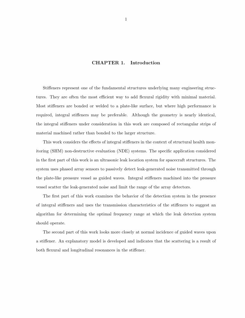
CHAPTER 1. Introduction
Stiffeners represent one of the fundamental structures underlying many engineering struc-
tures. They are often the most efficient way to add flexural rigidity with minimal material.
Most stiffeners are bonded or welded to a plate-like surface, but where high performance is
required, integral stiffeners may be preferable. Although the geometry is nearly identical,
the integral stiffeners under consideration in this work are composed of rectangular strips of
material machined rather than bonded to the larger structure.
This work considers the effects of integral stiffeners in the context of structural health mon-
itoring (SHM) non-destructive evaluation (NDE) systems. The specific application considered
in the first part of this work is an ultrasonic leak location system for spacecraft structures. The
system uses phased array sensors to passively detect leak-generated noise transmitted through
the plate-like pressure vessel as guided waves. Integral stiffeners machined into the pressure
vessel scatter the leak-generated noise and limit the range of the array detectors.
The first part of this work examines the behavior of the detection system in the presence
of integral stiffeners and uses the transmission characteristics of the stiffeners to suggest an
algorithm for determining the optimal frequency range at which the leak detection system
should operate.
The second part of this work looks more closely at normal incidence of guided waves upon
a stiffener. An explanatory model is developed and indicates that the scattering is a result of
both flexural and longitudinal resonances in the stiffener.
2
CHAPTER 2. Guided plate wave scattering at vertical stiffeners and its
effect on source location
Accepted for publication in ULTRASONICS October 26, 2011
R. S. Reusser, D. E. Chimenti, R. A. Roberts, S. D. Holland
Center for Nondestructive Evaluation
and Aerospace Engineering Department
Iowa State University
Ames IA 50011 USA
2.1 Abstract
This paper examines guided wave transmission characteristics of plate stiffeners and their
influence on the performance of acoustic noise source location. The motivation for this work is
the detection of air leaks in manned spacecraft. The leaking air is turbulent and generates noise
that can be detected by a contact-coupled acoustic array to perform source location and find
the air leak. Transmission characteristics of individual integral stiffeners are measured across
a frequency range of 50 to 400 kHz for both high and low aspect-ratio rectangular stiffeners,
and comparisons are made to model predictions which display generally good agreement. It
is demonstrated that operating in frequency ranges of high plate wave stiffener transmission
significantly improves the reliability of noise source location in the plate. A protocol is presented
to enable the selection of an optimal frequency range for leak location.
3
2.2 Introduction
Stiffeners are used in aerospace structures to add structural rigidity with minimal additional
weight. In situ structural health monitoring (SHM) non-destructive evaluation (NDE) systems
use ultrasonic guided waves to evaluate structural integrity (1). The interaction of guided
waves with structural features limits the range of ultrasonic SHM sensors. Typical NDE and
SHM applications use piezoelectric actuators to excite guided wave modes in the kilohertz to
low-megahertz range. The waves propagate through the structure, and after interacting with
a feature of interest, they propagate to a detector. Analysis of the detected waveforms gives
information on structural degradation. Thus, the interaction of guided waves with lap joints
(2; 3), stringers (6), more complex joints (13), or integral stiffeners controls the amount of
energy that eventually reaches the detector.
This paper considers the influence of rectangular stiffeners typical in spacecraft structures
on guided plate wave propagation. This type of integral stiffener is machined directly into the
structure in order to add flexural rigidity with minimal weight. Many studies have consid-
ered the similar problems of guided wave reflection from rectangular notches (6; 2; 7; 8), step
thickness changes (9), or strip weldments (10). Wilcox et al. analyze an adhesively bonded
stringer using the Semi-Analytical Finite Element method and observe variation in guided wave
transmission as the incident angle of waves upon the straight feature is varied (6). We show
here, based on experimental data and Boundary Element Method (BEM) simulations (4), that
rectangular stiffening ribs act like a geometric filter, producing some frequency bands with high
transmission across stiffeners, and other frequency bands with low transmission. This filtering
behavior limits performance of an SHM systems such as ours that locates leaks in manned
4
spacecraft.
2.2.1 Spacecraft Leak Location
Manned spacecraft are at risk of orbital debris and micrometiorite impact (12; 13) which
can generate an air leak. Because of the limited oxygen on board, it is imperative to quickly
locate a leak. Turbulence-generated airborne noise is the conventional method of locating leaks
in pressure vessels. In space, because the air leaks into the vacuum, the leak noise flows outward
with the air and there is almost no airborne noise generated inside the spacecraft. In addition,
equipment and life support systems mounted against the pressure vessel wall inhibit access and
preclude rapid location of an air leak. The method we have reported (14) relies instead on ultra-
sonic noise (20-400 kHz) generated by the leak in the skin of the spacecraft structure, through
aerodynamic coupling of the escaping air to the plate-like pressure vessel wall. An acoustic
array provides directional information on the arriving noise signals. Temporal correlations ex-
tract the statistics of the noise signal arriving at one array element compared to signals from all
the other elements of the array (15). Because the signals are random and continuous, the signal
acquisition and processing can proceed sequentially, significantly reducing the expense of the
electronics. Extension of the two-dimensional spatio-temporal analysis of Alleyne and Cawley
(16) to three dimension transforms the measured correlations into frequency-wavevector space.
The direction of the wavevector under the sensor array indicates the direction to the noise
signal source. Triangulation with two or more arrays locates the leak.
Successful leak location has been demonstrated on simulated spacecraft structure using a
64-element diced PZT (lead zirconate titanate) piezoelectric array detector (17). Our own prior
work (14; 18) has shown that integral stiffeners may limit performance of the leak location pro-
5
cedure. In an environment where prompt and accurate leak location is critical, the system and
procedure must be robust, so the current work focuses on a study of guided wave propagation in
spacecraft structures to evaluate stiffener transmission characteristics, and uses those results to
develop a frequency selection protocol for optimal detection center frequency and bandwidth.
We find that guided wave transmission measurements performed at normal incidence using
a piezoelectric point source and an ideal optical virtual array receiver are consistent with BEM
simulations over a frequency range of 50 to 400 kHz for two types of stiffener geometry. Since
the transmission varies greatly with frequency, and the location of the passbands (transmitted
frequencies) are strongly geometry-dependent, it is best to include the entire frequency range
in the active analysis. When integrated over the entire detection spectrum, the passbands
dominate the other frequencies, producing accurate results.
2.3 Transmission across a Stiffener
The theory of guided Lamb waves is well known (9). Geometric obstructions, such as
the integral stiffeners considered here, scatter guided Lamb modes, resulting in reflection and
transmission as well as mode conversion of an incoming wave. The reflection and transmission
depend on frequency, aspect ratio, guided wave mode, and incident angle. The stiffener acts
as a geometry-dependent filter of the guided wave; It is observed that certain frequency bands
have high transmission and other frequency bands have high reflection (5). Transmission across
the stiffener seems to be related to resonances which, in the case of non-normal incidence, map
to feature-guided waves that propagate along the stiffener (6).
6
2.3.1 Theory
A single guided mode incident upon a stiffener may be mode-converted into multiple scat-
tered modes. The overall behavior is represented with an energy transmission coefficient,
defined at frequency ω by
T (ω) =
∑nEtr
n (ω)∑nEinc
n (ω), (2.1)
where Etrn and Einc
n are the transmitted and incident energies of the nth guided wave modes,
respectively. Because the A0 and S0 modes are the only propagating modes that exist at low
frequency, and because the A0 mode dominates over the symmetric mode under the asym-
metric excitation used in our experiments, only the A0 mode need be considered. With that
simplification, the transmission coefficient is
T (ω) ≈Etr
A0(ω)
EincA0
(ω). (2.2)
Observing that energy is proportional to the square of amplitude, the expression can further
be simplified to
T (ω) =|Atr
A0(ω)|2
|AincA0
(ω)|2 . (2.3)
2.3.2 Experiment
To measure transmission of the lowest order antisymmetric, or A0, Lamb mode across an
integral stiffener, a laser vibrometer measures modal amplitudes of incident and transmitted
guided waves created by a piezoelectric contact transducer. The methodology is similar to that
of Morvan et al. (11) to study Lamb wave reflection from the free edge of a plate, and has been
used extensively for SHM applications (22; 23; 24). Because the guided wave amplitude will be
a superposition of incident and reflected waves as well as waves reflected from the boundaries,
7
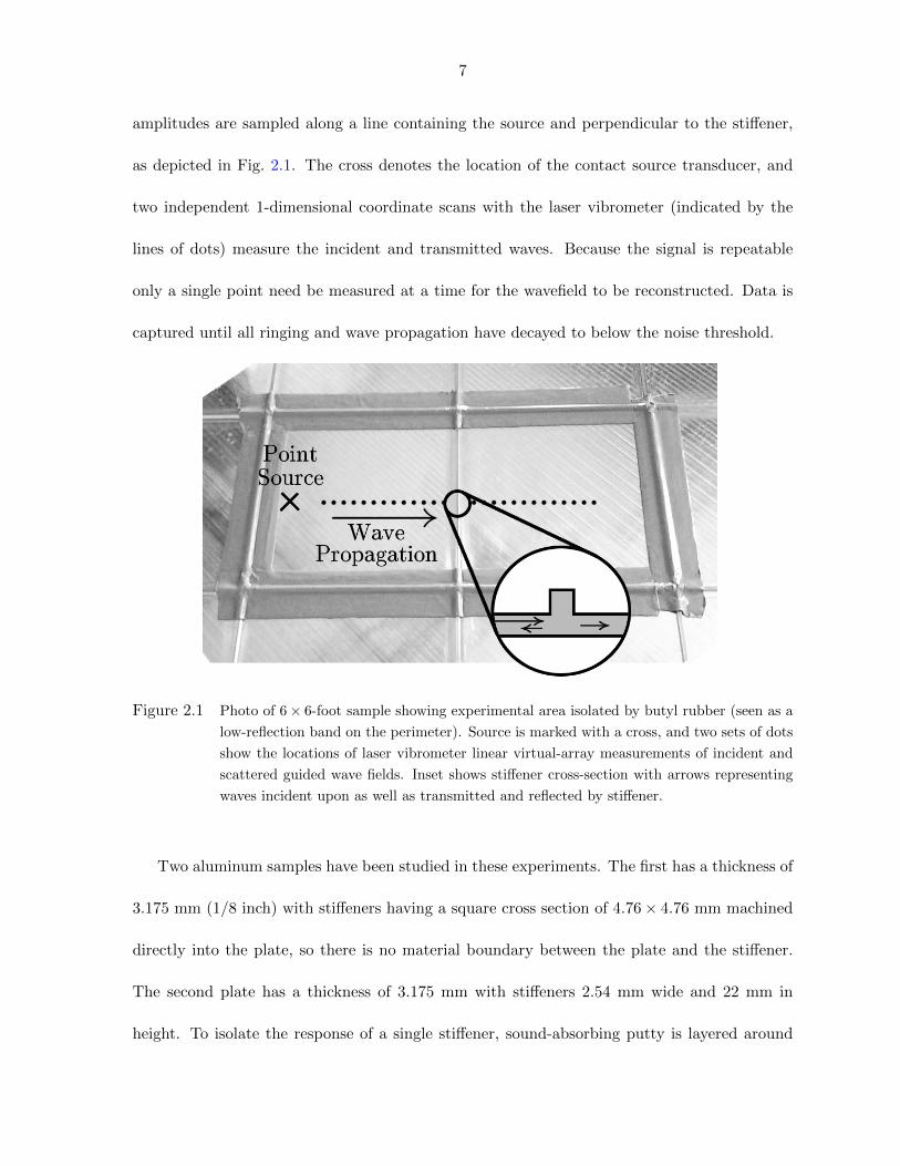
amplitudes are sampled along a line containing the source and perpendicular to the stiffener,
as depicted in Fig. 2.1. The cross denotes the location of the contact source transducer, and
two independent 1-dimensional coordinate scans with the laser vibrometer (indicated by the
lines of dots) measure the incident and transmitted waves. Because the signal is repeatable
only a single point need be measured at a time for the wavefield to be reconstructed. Data is
captured until all ringing and wave propagation have decayed to below the noise threshold.
Figure 2.1 Photo of 6× 6-foot sample showing experimental area isolated by butyl rubber (seen as a
low-reflection band on the perimeter). Source is marked with a cross, and two sets of dots
show the locations of laser vibrometer linear virtual-array measurements of incident and
scattered guided wave fields. Inset shows stiffener cross-section with arrows representing
waves incident upon as well as transmitted and reflected by stiffener.
Two aluminum samples have been studied in these experiments. The first has a thickness of
3.175 mm (1/8 inch) with stiffeners having a square cross section of 4.76× 4.76 mm machined
directly into the plate, so there is no material boundary between the plate and the stiffener.
The second plate has a thickness of 3.175 mm with stiffeners 2.54 mm wide and 22 mm in
height. To isolate the response of a single stiffener, sound-absorbing putty is layered around
8
the perimeter of the experimental area so that reflections are almost completely suppressed,
even at the lowest frequency of 50 kHz. A representation of the experimental geometry is shown
in the inset of Fig. 2.1. The incident, reflected, and transmitted waves are shown for the short,
or low aspect-ratio, stiffener.
A 9.5-mm diameter contact transducer with a non-resonant ultrasonic horn that reduces
the contact area to roughly 1 mm2 induces guided waves in the plates. A Panametrics
pulser/receiver excites the transducer, which is fixed to the specimen with couplant and light
pressure for the duration of the test. Because of asymmetric single-side excitation, most of the
energy resides in the A0 Lamb mode.
At each point in the scan, a Polytec OFV-5000/OFV-505 Laser Vibrometer measures the
out-of-plane particle velocity of the plate surface. At the frequencies involved, the sensitivity
of the laser vibrometer is very poor compared piezoelectric sensors. The point contact horn
on the source transducer best approximates a point source, but is inefficient. Because of these
conditions, 104 averaged impulse responses at a simulated leak source acquired at a rate of 100
Hz, provide the desired signal-to-noise ratio. To achieve the best results, the full usable spans
of the plates are scanned with 1 mm spacing.
To correct for radial falloff of the waves as they spread in two dimensions, the signal measure-
ments are normalized by 1/√r, where r is the distance from the noise source to the measurement
location. A spatio-temporal Fourier transform of the measured signal (16; 25), permits separa-
tion of the modes and guided wave propagation directions in frequency-wavenumber space. A
spatial Kaiser window applied before the Fourier transform reduces sidelobes. Finally, ampli-
tudes are sampled along the incident and transmitted A0 mode curves, and the transmission
coefficient is calculated per frequency with Eq. (3.42).
9
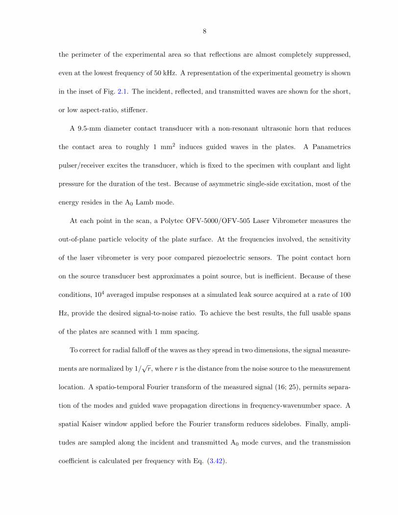
Figure 2.2 Measured normal component of particle velocity magnitude displayed as a gray-scale plot
in coordinate x and time t for the tall stiffener test section. The wave amplitude is
represented by the surface particle velocity vn
Figure 2.2 illustrates a portion of the measured x − t diagram for scattering from the tall
stiffener. The magnitude of the normal component of the velocity magnitude is plotted in a
logarithmic gray-scale (higher amplitude, darker value) in time from t = 0 to t = 250µs and in
space from the source at x = 0 to the stiffener at x = 325 mm and beyond out to 550 mm from
the source, both segments acquired with 1 mm spacing. Visible in the data are the incident
S0 and A0 modes. Although the A0 mode has greater out of plane velocity than the S0 mode for
a given energy flux, the incident energy flux of the S0 mode is still only ten percent that of the
A0 mode at the center frequency (200 kHz). A portion of the incident S0 energy mode converts
to A0. When the stronger but slower incident A0 waves meet the stiffener, there is significant
10
0.00 0.05 0.10 0.15 0.20 0.25 0.30 0.35 0.40
Wavenumber, k, mm−1
0
200
400
600
800
1000
1200
Fre
quen
cy,f
,kH
z
A0S0
A1
S1
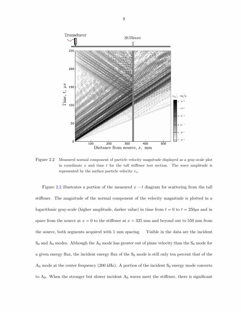
Figure 2.3 Measured dispersion curves for incident guided plate waves in the high aspect-ratio test
section. Calculate Lamb wave dispersion curves (dotted lines) are superimposed.
reflection and transmission of energy with little conversion. A very close examination shows
that a small amount of A0 →S0 mode conversion does occur in the transmitted waves, but it
amounts to only 5% of the incident energy flux.
Interestingly, on the left side of the figure the vibrometer detects a very faint, and very
slow, acoustic wave which appears as a faint line from the source to about 80 mm at t = 250µs.
The wave speed matches the 340 m/s speed an acoustic wave travels in air.
The measured incident wave spectrum, the 2-D Fourier transform of the data of Fig. 2.2,
is shown in Fig. 2.3. The data fall onto discrete mode curves which coincide with normal
modes of the plate, i.e., Lamb waves. The spectrum of the source transducer together with
the amount of out-of-plane moton for a given mode and frequency determines the magnitude
at each point on the dispersion curves. Higher normal wave motion leads to a larger detected
11
amplitude, such as between 100 and 300 kHz and 0.05 to 0.15 mm−1 in the wavenumber for
the A0 mode. Between 600 and 900 kHz the lowest order symmetric mode S0 is also rather
strongly excited, but very little of the S0 mode is seen below 500 kHz.
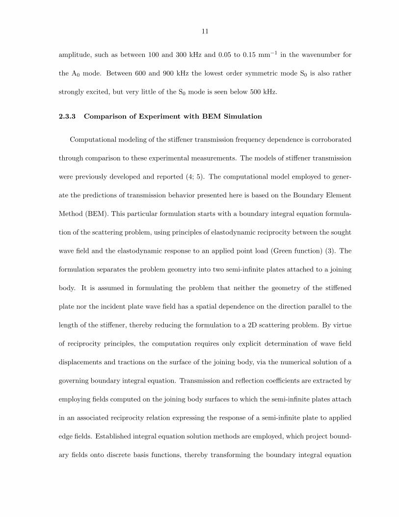
2.3.3 Comparison of Experiment with BEM Simulation
Computational modeling of the stiffener transmission frequency dependence is corroborated
through comparison to these experimental measurements. The models of stiffener transmission
were previously developed and reported (4; 5). The computational model employed to gener-
ate the predictions of transmission behavior presented here is based on the Boundary Element
Method (BEM). This particular formulation starts with a boundary integral equation formula-
tion of the scattering problem, using principles of elastodynamic reciprocity between the sought
wave field and the elastodynamic response to an applied point load (Green function) (3). The
formulation separates the problem geometry into two semi-infinite plates attached to a joining
body. It is assumed in formulating the problem that neither the geometry of the stiffened
plate nor the incident plate wave field has a spatial dependence on the direction parallel to the
length of the stiffener, thereby reducing the formulation to a 2D scattering problem. By virtue
of reciprocity principles, the computation requires only explicit determination of wave field
displacements and tractions on the surface of the joining body, via the numerical solution of a
governing boundary integral equation. Transmission and reflection coefficients are extracted by
employing fields computed on the joining body surfaces to which the semi-infinite plates attach
in an associated reciprocity relation expressing the response of a semi-infinite plate to applied
edge fields. Established integral equation solution methods are employed, which project bound-
ary fields onto discrete basis functions, thereby transforming the boundary integral equation
12
into an algebraic matrix equation, variously referred to as the Method of Moments (MoM), or
the Boundary Element Method (BEM) (27; 2). A more detailed exposition of the computa-
tional model used to generate the results presented here is found in (4). Others methods have
been applied to plate wave transmission at a geometric disruption, such as application of Finite
Element Analysis (6). The benefit of a semi-analytical approach such as the one used here is
that the semi-infinite plates can be modeled explicitly.
Application of the computational model to the stiffened plate defines the joining body to
consist of the stiffening rib plus the adjacent section of the plate to which the stiffening rib
is integrally attached (see Figure 2.1). The surface of the joining body is sub-divided into
adjacent boundary segments, over each of which the sought wave field is represented as a
quadratic polynomial. Employing this field representation in the governing boundary integral
equation yields a matrix equation for the polynomial coefficients. For the low aspect ratio
stiffener (4.76× 4.76 mm), 5 boundary segments were prescribed on each face of the stiffener,
and on each plate attachment surface, yielding a total of 30 segments. Three polynomial
coefficients for the 2D wave field on each segment results in a 180 × 180 coefficient matrix,
the inversion of which yields the desired field on the plate attachment surfaces. The width
and height of the high aspect ratio stiffener (2.54 × 22 mm) was subdivided into 2 and 15
segments, respectively, with 5 segments prescribed over the plate attachment surfaces, leading
to inversion of a 264 × 264 coefficient matrix. Applying the computed plate attachment wave
field to the edge of the semi-infinite plate and employing field reciprocity as described in (5)
yields computed versions of the guided wave transmission coefficients referred to in Eq. (3.42).
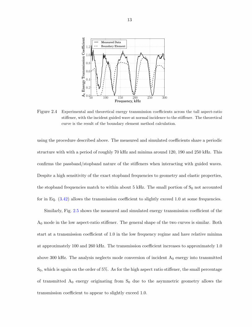
Fig. 2.4 shows measured and simulated transmission coefficients of a high aspect ratio
stiffener. The measured coefficient is calculated from data in Fig. 2.2 to evaluate Eq. (3.42)
13
50 100 150 200 250 300Frequency, kHz
0.0
0.2
0.4
0.6
0.8
1.0
1.2
A0
Ene
rgy
Tra
nsm
issi
onC
oeffi
cien
t
Measured DataBoundary Element
Figure 2.4 Experimental and theoretical energy transmission coefficients across the tall aspect-ratio
stiffener, with the incident guided wave at normal incidence to the stiffener. The theoretical
curve is the result of the boundary element method calculation.
using the procedure described above. The measured and simulated coefficients share a periodic
structure with with a period of roughly 70 kHz and minima around 120, 190 and 250 kHz. This
confirms the passband/stopband nature of the stiffeners when interacting with guided waves.
Despite a high sensitivity of the exact stopband frequencies to geometry and elastic properties,
the stopband frequencies match to within about 5 kHz. The small portion of S0 not accounted
for in Eq. (3.42) allows the transmission coefficient to slightly exceed 1.0 at some frequencies.
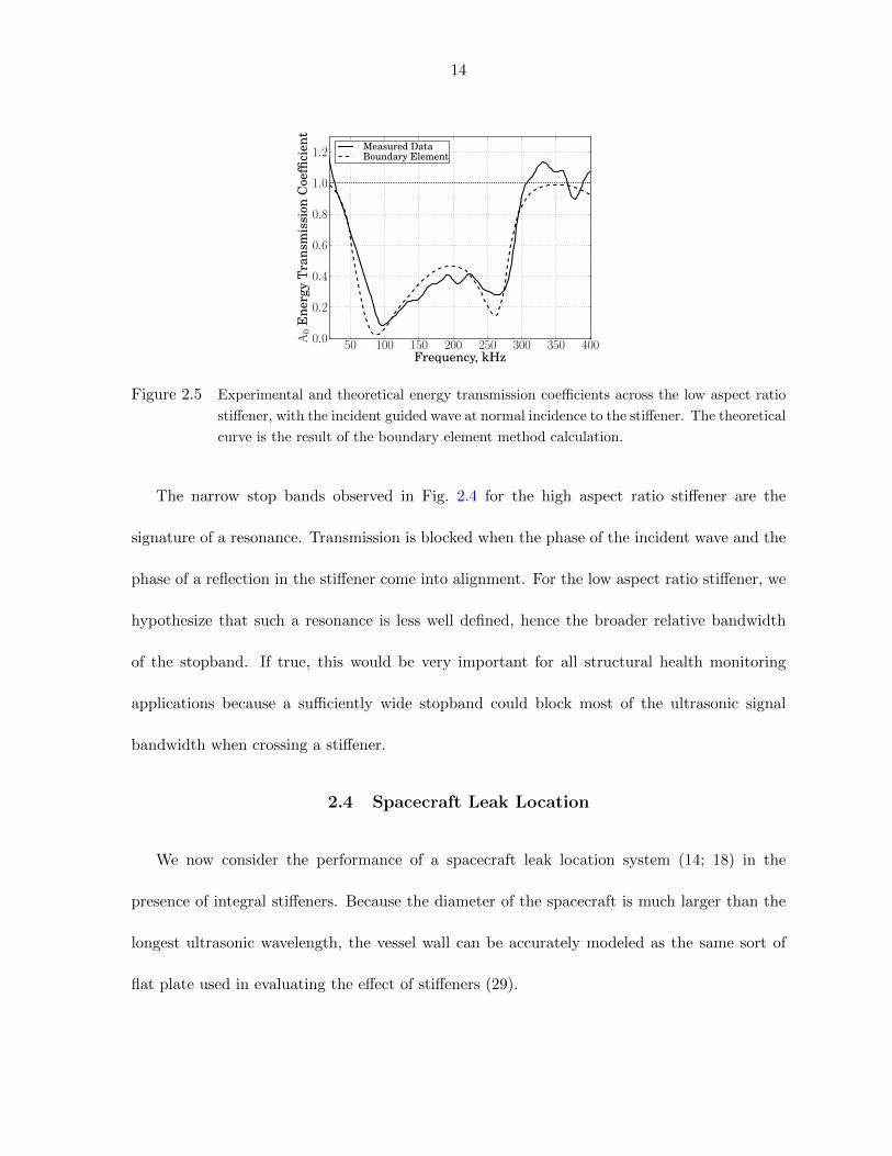
Similarly, Fig. 2.5 shows the measured and simulated energy transmission coefficient of the
A0 mode in the low aspect-ratio stiffener. The general shape of the two curves is similar. Both
start at a transmission coefficient of 1.0 in the low frequency regime and have relative minima
at approximately 100 and 260 kHz. The transmission coefficient increases to approximately 1.0
above 300 kHz. The analysis neglects mode conversion of incident A0 energy into transmitted
S0, which is again on the order of 5%. As for the high aspect ratio stiffener, the small percentage
of transmitted A0 energy originating from S0 due to the asymmetric geometry allows the
transmission coefficient to appear to slightly exceed 1.0.
14
50 100 150 200 250 300 350 400Frequency, kHz
0.0
0.2
0.4
0.6
0.8
1.0
1.2
A0
Ene
rgy
Tra
nsm
issi
onC
oeffi
cien
t
Measured DataBoundary Element
Figure 2.5 Experimental and theoretical energy transmission coefficients across the low aspect ratio
stiffener, with the incident guided wave at normal incidence to the stiffener. The theoretical
curve is the result of the boundary element method calculation.
The narrow stop bands observed in Fig. 2.4 for the high aspect ratio stiffener are the
signature of a resonance. Transmission is blocked when the phase of the incident wave and the
phase of a reflection in the stiffener come into alignment. For the low aspect ratio stiffener, we
hypothesize that such a resonance is less well defined, hence the broader relative bandwidth
of the stopband. If true, this would be very important for all structural health monitoring
applications because a sufficiently wide stopband could block most of the ultrasonic signal
bandwidth when crossing a stiffener.
2.4 Spacecraft Leak Location
We now consider the performance of a spacecraft leak location system (14; 18) in the
presence of integral stiffeners. Because the diameter of the spacecraft is much larger than the
longest ultrasonic wavelength, the vessel wall can be accurately modeled as the same sort of
flat plate used in evaluating the effect of stiffeners (29).
15
2.4.1 Theory
To summarize the guided wave source location method briefly, the signal generated by the
source and arriving at the jth element of the detector array can be expressed, for distance
|xj | � 1/kn(ω), as
v(xj , ω) = N(ω)|xj |−1/2∑n
An(ω) exp(i kn(ω)|xj |), (2.4)
where v represents the normal particle velocity at the jth array element at position xj and
frequency ω to be measured with the laser vibrometer. The term N represents the complex
amplitude and phase of the source, and the propagating waves are summed over all guided
wave modes n with amplitude coefficient An. We can represent the jth array element vector
position xj as the sum of the array reference position x0 and a relative element position sj ,
xj = x0 + sj . (2.5)
The distance to a specific element can be written using the far-field approximation as
|xj | = |x0|+ d · sj , (2.6)
where d is a unit vector representing the direction of wave propagation under the array. Then,
substitution into Eq. 2.4 yields
v(xj , ω) = N(ω)|x0|−1/2∑n
An(ω) exp [i kn(ω)(|x0|+ d · sj)] . (2.7)
The detector array (PZT or laser vibrometer) is not infinitely large, so its finite spatial ex-
tent means that a spatial window function W (x) is applied to the acquired data. The two-
dimensional Fourier transform of Eq. 2.7 in transform variables k and ω gives
FT {W (x)v(x, ω)} =∑n
Bn W (k− knd) , (2.8)
16
where W is the Fourier-transformed window function and the amplitude coefficients have been
grouped into Bn which is implicitly dependent on frequency. Representing the data in a two-
dimensional wavenumber map, the energy in all modes n and at frequency ω lies along a line
emanating from the origin and in the dominant direction of wave propagation d. This direction
can then be discerned by inspection of the map. Summing over a particular frequency range
∆ω enhances the detectability of the leak. This operation results in a much improved detection
accuracy and a more robust leak location method. Suppressing the parametric dependence on
frequency ω and local array vector s, we have
ω2∑ω1
FT {W v} =
ω2∑ω1
∑n
Bn W (k− knd) . (2.9)
That is to say, the 3-D spatio-temporal (x, y, t) Fourier transform of the measured detector
array data, summed over the relevant frequency band, gives a map of the propagating waves
under the array in terms of k = (kx, ky), blurred by the limited spatial sensing range and
windowing. The above analysis makes no assumptions about the wave source. The noise from
the leak (our desired “signal”) is in fact random, but we cross correlate it, which makes it
deterministic. In most ultrasonic experiments, we time gate our detection to eliminate the
interference from late arrivals. With the correlated random source, this is not possible. In the
experiments below we have done sufficient averageing that the “noise” we are fighting comes
not from the detector but instead from interference from alternate wave paths.
2.4.2 An Algorithm for Selecting a Frequency Band
Selection of the proper frequency band is critical to determining the most probable leak
location and minimizing the number of required sensors. Three factors determine this frequency
band: leak noise spectrum, array detector sensitivity, and noise transmission across structural
17
features. A robust leak location system must operate in the intersection of these three criteria.
Basic turbulence theory predicts the leak energy coupled into the plate will decrease with
frequency (30), and in fact it is observed that no usable leak noise lies beyond roughly 400 kHz.
This finding matches the sensitivity of the detector, which operates up to 500 kHz. Thus the
useful noise for spacecraft leak location is noise below 400 kHz which is minimally scattered by
the spacecraft structure.
The most straightforward algorithm for locating the high transmission frequencies, termed
in situ calibration, collocates a simulated leak with each detector array. The calibration is
determined by sensing the simulated leak signal from each of the other non-collocated detector
arrays. Location of one simulated leak at a time with each of the other sensors determines the
calibration. The disadvantage of this method is that it requires additional complexity, power,
and cost of additional source transducers. to act as simulated leaks. The second method,
termed wide-bandwidth analysis, simply uses the full functional range of the array detector.
By integrating over all available frequencies that may provide a correct answer, those frequencies
that transmit through stiffeners tend to dominate the measured signals.
2.4.3 Experimental Configuration
A 6×6 foot plate containing a 1 foot grid of low aspect-ratio stiffeners simulates a section of
a spacecraft pressure vessel. (A small section of the same plate was used for the low aspect-ratio
stiffener transmission measurement in Section 2.) Forty-three different simulated leak locations
have been arbitrarily distributed across the surface of the plate. The point contact transducer
is excited with a Panametrics pulser/receiver in a manner identical to the stiffener transmission
tests.
18
The laser vibrometer virtual array consists of a 12 × 12 scanned point array on a 27.5 ×
27.5 mm area with 2.5 mm spacing between the optical beam points. The out-of-plane motion
is captured with the laser vibrometer using 200 triggers per point, averaged. Waveforms at
each point are acquired sequentially and the direction of wave propagation is determined from
Eq. 2.9. Fewer averages are needed here than the 104 needed for the stiffener transmission mea-
surement because the very high signal-to-noise ratio is not required and because the measured
response can be integrated over frequency. Throughout the tests, the optical array location
is not moved. Instead, the piezoelectric source transducer is attached to the plate with mild
pressure and a very thin layer of butyl rubber for acoustic coupling and is moved to simulate
different leak locations relative to the stiffener.
The results of one of the simulated in situ calibration tests are plotted in Fig. 2.6. The
spatial Fourier transform is zero-padded to 128×128 points in the x and y directions and uses a
rectangular window. Each data point in the plot has been integrated with a 25-kHz bandwidth
from 75 to 100 kHz. After summing, the data is integrated along a set of radial lines with
0.5◦ resolution. The angle with the largest integral is selected and plotted at each source point
with a solid line. Each “x” in the figure corresponds to a simulated leak location, and the
single circle shows the location on the 6 × 6-foot plate of the scanned laser vibrometer array.
The arrows at each “x” correspond to the most likely direction of the arriving wave vector, as
measured at the open circle. The arrow lengths have been scaled for ease of interpetation so
they nearly reach the detector. The diagonal dashed lines represent the low aspect-ratio integral
stiffeners. Figure 2.6 shows the results of all 43 tests with the wavenumber map integrated over
a frequency range extending from 75 to 100 kHz, as described in (14). For each test, only the
strongest observed wavevector has been sampled and plotted. Although some of the simulated
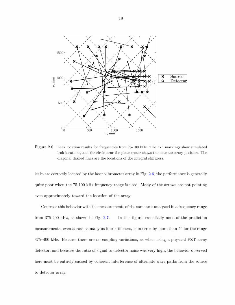
19
0 500 1000 1500x, mm
0
500
1000
1500y,m
m
SourceDetector
Figure 2.6 Leak location results for frequencies from 75-100 kHz. The “x” markings show simulated
leak locations, and the circle near the plate center shows the detector array position. The
diagonal dashed lines are the locations of the integral stiffeners.
leaks are correctly located by the laser vibrometer array in Fig. 2.6, the performance is generally
quite poor when the 75-100 kHz frequency range is used. Many of the arrows are not pointing
even approximately toward the location of the array.
Contrast this behavior with the measurements of the same test analyzed in a frequency range
from 375-400 kHz, as shown in Fig. 2.7. In this figure, essentially none of the prediction
measurements, even across as many as four stiffeners, is in error by more than 5◦ for the range
375–400 kHz. Because there are no coupling variations, as when using a physical PZT array
detector, and because the ratio of signal to detector noise was very high, the behavior observed
here must be entirely caused by coherent interference of alternate wave paths from the source
to detector array.
20
0 500 1000 1500x, mm
0
500
1000
1500y,m
m
SourceDetector
Figure 2.7 Leak location results for frequencies in the range 375–400 kHz. The “x” markings show
simulated leak locations, and the circle shows the detector array position. The diago-
nal dashed lines are the integral stiffeners. The arrows, indicating the predicted source
directions based on the measured data, are now essentially all correct.
These observations using the laser vibrometer detector match very closely the measured
performance of the PZT array detector, when it is also operated in this frequency range.
Furthermore, these results are completely consistent with the stiffener transmission coefficients
in Fig. 2.5. In tests with either the laser vibrometer or PZT array, leak location occurs with
consistent accuracy mainly above 275 kHz. Although the test data shown in Fig. 2.7 indicate
clearly that the guided wavevectors are not always normal to the stiffener, as they are in the
transmission coefficients plotted in Fig. 2.5, the data of Fig. 2.7 strongly suggest that normal-
incidence transmission still is a good indicator of leak location performance.
The strong correlation described above between stiffener transmission and accurate leak
21
0 500 1000 1500x, mm
0
500
1000
1500y,m
m
SourceDetector
Figure 2.8 Normalized leak location maps for frequencies in the range 100–475 kHz. The “x” markings
show simulated leak locations, and the circle shows the detector array position. The
diagonal dashed lines are the integral stiffeners. The arrows, indicating the predicted
source directions based on the measured data, are still nearly all correct, as they were in
Fig. 2.7.
location seems to favor in situ calibration as the preferable algorithm for frequency range
selection. Not all stiffener geometries, however, have such wide passbands and stopbands. For
the tall stiffener (2.54 mm wide by 22 mm high) Fig. 2.4 shows the measured and calculated
transmission coefficients, but with much narrower passbands and stopbands. Moreover at non-
normal incidence the frequencies can scale or shift, which could lead to an absence of any
frequency bands with consistently good transmission.
In fact, there is no real need to choose such a narrow frequency band. Figure 2.8 shows
data from the same tests as those presented in Figs. 2.6–2.7, but with the maps normalized
so as to weight all frequencies equally when integrated from 100 to 475 kHz. Normalization
22
prevents a single spurious frequency from dominating the entire result. This wide-bandwidth
algorithm demonstrates accurate leak location for 40 of the 43 tests. Although this result does
not quite match the nearly perfect performance of Fig. 2.7, it does demonstrate that a simpler,
more robust strategy can still locate leaks with high accuracy. For a practical array, which
will not have flat frequency response, the response could similarly be normalized, within the
constraints of detector noise. To compensate for that dependence, which can include coupling
variations and wave damping, we would need to reformulate the protocol to give extra weight
to those frequency ranges where the signal is stronger owing to these extrinsic effects.
2.5 Summary and conclusions
Measurements and simulations have shown that integral stiffeners pass ultrasonic waves in
some frequency bands while almost entirely blocking them in others. High aspect ratio stiff-
eners seem to block transmission at their resonance. BEM simulations accurately predict this
stopband/passband behavior, despite the sensitivity of the stopband and passband frequencies
to stiffener height and elastic properties. As a result of these stopbands and their variation in
frequency with incident angle, it will be best to take advantage of all available frequencies in
finding the direction to the leak source. Further investigations might include the examination
of the angular dependence of guided wave transmission and mode conversion at off-normal
incidence on an integrally stiffened plate.
ACKNOWLEDGEMENT
This work is partially funded under NASA STTR #NNJ08JD11C through subcontract
#2008-08-307 with Invocon, LLC.
23
Bibliography
[1] A. Raghavan, C. E. S. Cesnik, “Review of Guided-wave Structural Health Monitoring,”
The Shock and Vibration Digest 39(2), pp. 91-114, (2007).
[2] M. J. S. Lowe, R. E. Challis, C. W. Chan, “The transmission of Lamb waves across
adhesively bonded lap joints,” J. Acoust. Soc. Am. 107(3), pp. 1333-1345, (2000).
[3] E. Lindgren, K. Jata, B. Scholes, J. Knopp, “Ultrasonic plate waves for fatigue crack
detection in multi-layered metallic structures,” Proc. SPIE 6532, 653207 (2007).
[6] P. Wilcox, A. Velichko, B. Drinkwater, A. Croxford, “Scattering of plane guided waves
obliquely incident on a straight feature with uniform cross-section,” J. Acoust. Soc. Am.
128(5), pp. 2715-2725, (2010).
[13] D. W. Greve, N. Tyson, I. J. Oppenheim, “Interaction of defects with Lamb waves in
complex geometries,” IEEE Ultrasonics Conference Proceedings, 297-300, (2005).
[6] B. A. Auld, M. Tan, “Symmetrical Lamb Wave Scattering at a Symmetrical Pair of Thin
Slots,” Ultrasonics Symposium, pp. 61-66, (1977).
[7] F. Benmeddour, S. Grondel, J. Assaad, Emmanuel Moulin, “Study of the fundamental
Lamb modes interaction with symmetrical notches,” NDT & E International 41, pp. 1-9,
(2008).
24
[8] A. Demma, P. Cawley, M. J. S. Lowe, “Scattering of the fundamental shear horizontal
mode from steps and notches in plates,” J. Acoust. Soc. Am., 113(4), pp. 1880-1891,
(2003).
[9] Y. Cho, “Estimation of ultrasonic guided wave mode conversion in a plate with thick-
ness variation,” IEEE Transactions on Ultrasonoics, Ferroelectrics, and Frequency Control
47(3), pp. 591-603, (2000).
[10] Y. N. Al-Nasser, S. K. Datta, A. H. Shah, “Scattering of Lamb waves by a normal rect-
angular strip weldment,” Ultrasonics, 29(2), pp. 125-132, (1991).
[4] R. A. Roberts, “Guided wave propagation in integrally stiffened plates,” in Review of
Progress in Quantitative Nondestructive Evaluation, vol. 27, D. O. Thompson, D. E.
Chimenti, Eds. (AIP Press, New York, 2008), pp. 170–177.
[12] D. S. F. Portree and J. P. Loftus, Jr, “Orbital debris: A chronology,” NASA Technical
Paper TP-1999-208856, (1999).
[13] D. J. Kessler, “Sources of orbital debris and the projected environment for future space-
craft,” J. Spacecraft 18, pp. 357-360, (1981).
[14] S. D. Holland, D. E. Chimenti, R. A. Roberts, and M. Strei, “Locating air leaks in manned
spacecraft using structure-borne noise,” J. Acoust. Soc. Am. 121, pp. 3484–3492 (2007).
[15] S. M. Ziola, M. R. Gorman, “Source location in thin plates using cross-correlation,” J.
Acoust. Soc. Am. 90(5), pp. 2551-2556, (1991).
[16] D. Alleyne, P. Cawley, “A two-dimensional Fourier transform method for the measurement
of propagating multimode signals,” J. Acoust. Soc. Am, 89(3), pp. 1159-1168, (1991).
25
[17] S. D. Holland, R. A. Roberts, D. E. Chimenti, Jun-Ho Song, “An ultrasonic array sensor
for spacecraft leak direction finding,” Ultrasonics 45, pp. 121–126 (2006).
[18] S. D. Holland, R. A. Roberts, D. E. Chimenti, and M. Strei, “Leak detection in spacecraft
using structure-borne noise with distributed sensors,” Appl. Phys. Lett. 86, 174105-1–3
(2005).
[9] J. D. Achenbach, Wave propagation in elastic solids, American Elselvier, (1973).
[5] R. A. Roberts, “Plate wave transmission/reflection at geometric obstructions: model
study,” Review of Progress in Quantitative Nondestructive Evaluation, vol. 29, D. O.
Thompson, D. E. Chimenti, Eds. (AIP Press, New York, 2010), pp. 192–199.
[11] B. Morvan, N. Wilie-Chancellier, H. Duflo, A. Tinel, J. Duclos, “Lamb wave reflection at
the free edge of a plate” in J. Acoust. Soc. Am. 113(3), pp. 1417-1425, (2003).
[22] W. J. Staszewski, B. C. Lee, L. Mallet, F. Scarpa, “Structural health monitoring using
scanning laser vibrometry: I. Lamb wave sensing,” Smart Mater. and Struct., 13, pp.
251-260, (2004).
[23] L. Mallet, B. C. Lee, W. J. Staszewski, F. Scarpa, “Structural health monitoring using
scanning laser vibrometry: II. Lamb waves for damage detection,” Smart Mater. Struct.,
13, pp. 261-269, (2004).
[24] W. H. Leong, W. J. Staszewski, B. C. Lee, F. Scarpa, “Structural health monitoring using
scanning laser vibrometry: III. Lamb waves for fatigue crack detection,” Smart Mater.
Struct., 14, pp. 1387-1395, (2005).
[25] D. H. Johnson, Array Signal Processing: Concepts and Techniques, Prentice Hall, 1993.
26
[3] J. D. Achenbach, Reciprocity in Elastodynamics, (Cambridge Univ Press, London, 2003).
[27] W. C. Gibson, The Method of Moments in Electromagnetics. Chapman & Hall, CRC
Press, 2008.
[2] A. Cheng, D. Cheng, “Heritage and early history of the boundary element method,”
Engineering Analysis with Boundary Elements 29, pp. 268-302, (2005).
[29] D. C. Gazis, “Three-Dimensional Investigation of the Propagation of Waves in Hollow
Circular Cylinders. II. Numerical Results” J. Acoust. Soc. Am. 31(5), pp. 573-578, (1959).
[30] S. B. Pope, Turbulent Flows, (Cambridge University Press, London, 2000).
27
CHAPTER 3. Reflection and transmission of guided plate waves by
vertical stiffeners
R. S. Reusser, D. E. Chimenti, R. A. Roberts, S. D. Holland
Center for Nondestructive Evaluation
and Aerospace Engineering Department
Iowa State University
Ames IA 50011 USA
3.1 Abstract
The interaction of guided plate waves with integral stiffeners limits the spatial range of
structural health monitoring non-destructive evaluation systems. This paper develops a simple
explanatory model that illuminates the underlying mechanics of waves crossing a stiffener. The
model aids the designer and indicates transmission and reflection are determined by longitudinal
and flexural stiffener resonances. Good agreement is seen with numerical calculations using the
boundary element method and with experimental measurements.
28
3.2 Introduction
Stiffeners add flexural rigidity and buckling resistance to aerospace structures while mini-
mizing weight. Many structural health monitoring (SHM) non-destructive evaluation (NDE)
concepts rely on the ability of ultrasonic guided waves to propagate a long distance from actu-
ator to defect to detector in order to monitor structural integrity with a minimum of sensors
(1). Integral stiffeners interfere with propagating ultrasonic waves, limiting the effective range.
SHM sensors typically operate in kilohertz to low-megahertz range. Since useful wavelengths
are typically similar in length scale to the stiffeners, scattering is a complicated process that
results in a pattern of stopbands and passbands. Based on our observations and calculations,
guided wave transmission past an integral stiffener is determined by the pattern of resonances
within the stiffener.
Figure 3.1 shows the geometry for wave scattering by an integral stiffener. Incoming wave-
fronts parallel to the stiffener enter from the left. Upon interacting with the stiffener, a portion
of the waves are reflected back to the left, and the remaing energy is transmitted in waves
that exit to the right. Points representing the center of the junction (point J), the base of the
stiffener (point B), and the end of the stiffener (point E) are marked on the diagram.
Since scattering problems quickly becomes complex for non-trivial geometries, a great deal
of effort has been expended developing approximate and numerical solution techniques. The
most mathematically complete technique for linear elastic wave equations is the boundary
element method (BEM) (2) Using the Reciprocity theorem (3), the problem is reduced to an
integral discretized along the boundary of the geometry (4) (5). More recent developments
expand on the well-known finite element method (FEM) to improve the spectral properties of
29
Incident
Up
Down
Reflected Transmitted
Stiffener
J
E
B
Figure 3.1 Coordinate system for the stiffener cross-section, SHM transducer on the left trans-
mitting to an SHM receiver on the right.
solutions when dealing with propagating waves. These techniques are used very successfully to
analyze wave interaction with similar geometries (6). However, the downside of such numerical
techniques is that the complexity obscures the fundamental mechanics governing the problem.
Analytical approximations have been developed, but primarily for the cases of waves in
rods and rod impact. Lee and Kolsky (7) consider stress waves in circular rods as they pass
pass through an angular junction. By matching displacements and rotations at the joint, they
develop a theory that couples the two rods together and reproduces the experimentally observed
transmission and reflection of flexural and longitudinal waves. Yong and Atkins (8) also consider
transient wave propagation in square rods forming a T-junction, modeling the junction as a
rigid cube. Using Timoshenko beam theory, they observe good agreement with experiments
as longitudinal waves in the terminating rod approach a T-junction, pass through the joint,
and spread outward symmetrically. In a similar manner, we use the theory of guided waves
in plates to develop an approximate model for wave transmission past a stiffener. Through
a straightforward approximation and impedance techniques from transmission line theory, the
30
transmission coefficient is observed to be near unity at resonance (low stiffener mechanical
impedance) and near zero between resonances (high stiffener mechanical impedance.)
3.3 Approximate Model
3.3.1 High aspect ratio approxmation
The primary approximation in our model is that the aspect ratio of the stiffener is large
(much taller than it is thick). In this situation, the stiffener itself behaves as another plate.
Guided waves travel up and down it, interacting with the junction at one end and the free
surface at the other. The stiffener functions as a finite plate coupled to the larger plate.
Similarly, at some distance away from the stiffener, the waves traveling in the plate must
approach guided Lamb modes, for which an explicit solution and various approximations are
well known (9). The same holds in the stiffener away from either the junction or the free end.
Thus, the problem of guided wave scattering by a high aspect ratio stiffener is governed by the
interaction of guided Lamb modes with the junction and free end of the stiffener.
3.3.2 Small junction approximation
A number of exact solution techniques exist for Lamb wave reflection from the free edge of a
plate. Y. Cho combines a boundary element method with the normal mode expansion technique
(10), and Morvan et al. apply stress-free conditions at a number of colocation points along
the free edge (11). No such technique exists for the more complicated junction between plate
and stiffener. Typical approaches utilize numerical discretization, using either the Boundary
Element Method (BEM) (5) Finite Element Method (FEM) (12; 13), or, more recently, the
Semi-Analytical Finite Element (SAFE) method (6). These techniques are consistent, meaning
31
they approach the exact mathematical solution as grid resolution or discretization order are
increased, but at the cost of a great deal of computation. When the junction region is small
relative to wavelength of the guided plate waves, the precise mechanics of the junction become
less significant. As a result, the sections that meet at the junction may be though of as directly
coupled in displacement and rotation.
3.3.3 Low frequency approximation
The result of these approximations is that at low frequencies, the problem may be solved
through the combination of Lamb wave solutions with matching conditions where they meet.
This assumption leads to an approximate solution that still accurately captures the fundamental
mechanics of the scattering problem.
At low frequencies where translation and rotation of the stiffener cross section are more
significant than distortion, there are three primary degrees of freedom and corresponding forces
at each point along the plate. The state of the plate at a given point is defined by displacements
u =
u
v
θ
, (3.1)
where u is horizontal particle displacement, v is vertical displacement, and θ is counterclockwise
cross section rotation, and forces
F =
H
V
M
, (3.2)
where H is horizontal force per depth averaged across the cross-section, V is vertical force per
depth, and M is the moment per depth acting on the cross section.
32
3.3.4 Generalized Impedance
Forces in a linear dynamic system may be related to the resulting particle velocities through
a mechanical impedance, typically defined as
F = Zu, (3.3)
where F is force, Z is impedance (in N/(m/s)), and u is the time derivative of displacement u.
Impedance representation simplifies analysis, making the resulting transmission and reflection
coefficients relatively simple functions of impedance. This approach is commonly used in the
study of electronic transmission lines (14) where voltage and current are used in place of
force and particle velocity, respectively. Unlike electronic transmission lines when there is a
single force (voltage) and proportional degree of freedom (current), mechanical plates have
three forces (normal, shear, and moment) and three mechanical degrees of freedom (horizontal
velocity, vertical velocity, and rotational velocity). We can define a generalized impedance
matrix Z that relates the three forces to the three velocities,
F = Zu, (3.4)
where the bold symbols F and u indicate vectors of length 3, and Z is an 3×3 impedance matrix
coupling each degree of freedom to each of the forces. Writing out all components explicitly,H
V
M
=
z11 z12 z13
z21 z22 z23
z31 z32 z33
u
v
θ
. (3.5)
3.3.5 Junction
The free body diagram in Fig. 3.2 cuts the problem into three plates that meet at junction
J . The stiffener has a free end at point E. The subscript I/R indicates forces resulting from
33
HI/R,J
HT,J
HS,J
VI/R,JVT,J
VS,J
MI/R,J
MS,J
HS,E
VS,E
MS,E
MT,JIncident/Reflected Transmitted
Stiffener
(uS,E)
(vS,E)
(ÒS,E)
(uI/R,J)
(vI/R,J)
(ÒI/R,J) (uT,J)
(vT,J)
(ÒT,J)
(uS,J)
(vS,J)
(ÒS,J)
Figure 3.2 Free body diagram of the stiffener cross-section with corresponding displacements
in parentheses.
the superposition of incident and reflected waves, the subscript T indicates forces resulting
from transmitted waves, and the subscript S indicates forces resulting from the superposition
of waves traveling up and down the stiffener. All forces illustrated on the diagram indicate
complex amplitudes of time-harmonic forces at the cross section centers. These forces are
averaged across the cross section so that a single force at the cross-section center represents
the force applied to the whole cross-section.
Using these definitions, a guided wave of frequency f traveling in an unbounded plate may
be said to have a characteristic generalized impedance Z0 that fixes the relationship between
F and u for all types of waves the plate permits,
F = Z0u. (3.6)
34
3.3.6 Force Balance
If the three plates in Fig. 3.2 meet at a junction with no volume, then forces must balance
according to Newton’s 2nd Law, leading to the system of equations∑H = 0 : HI/R,J +HT,J +HS,J = 0∑V = 0 : VI/R,J + VT,J + VS,J = 0
x∑M = 0 : MI/R,J +MT,J +MS,J = 0,
(3.7)
or in vector notation using the definitions in Eqs. 3.1 and 3.2,
FI/R,J + FT,J + FS,J = 0. (3.8)
Since FI/R,J results from the superposition of incident and reflected waves, it can be split into
indicent and reflected components, yielding
FI,J + FR,J + FT,J + FS,J = 0. (3.9)
This force balance equation can be expressed in terms of the corresponding particle velocity
components and generalized impedances. If ZS is the generalized impedance representing the
total response of waves traveling up and down the stiffener, and Z0,I , Z0,R, and Z0,T are the
characteristic generalized impedance of incident, reflected, and transmitted waves respectively,
then by substitution into Eq. 3.9,
Z0,I uI,J + Z0,RuR,J + Z0,T uT,J + ZSuS,J = 0. (3.10)
uI/R,J here has been split by superposition into it’s right- and left-moving component,
uI/R,J = uI,J + uR,J . (3.11)
Displacements must also be continuous at the junction, so that
uT,J = uS,J = uI,J + uR,J . (3.12)
35
Using this fact, substitution and rearrangement of Eq. 3.10, noting that Z0,I = −Z0,T if the
plates on the left and right are the same, yields
uR,J = − (Z0,R + Z0,T + ZS)−1 ZSuI,J . (3.13)
Putting this equation in terms of incident and transmitted waves according to Eq. 3.11
yields
uT =(I− (Z0,R + Z0,T + ZS)−1 ZS
)uI , (3.14)
which, after rearrangement, becomes
uT = (Z0,R + Z0,T + ZS)−1 (Z0,R + Z0,T ) uI . (3.15)
Equation 3.15 expresses transmitted particle velocities in terms of incident particle velocities
and impedances. As is the case for most wave problems in bounded media though, guided plate
waves occur in a discrete set of modes.
3.3.7 Plate waves
The theory of guided plate waves is well known and studied (15; 9). The exact theory
due to Lamb describes dispersion of guided waves in a linear elastic isotropic plate. Figure
3.3 shows the dispersion curves of the first three guided Lamb modes for a 6061-T6 aluminum
alloy plate with measured longitudinal wave speed 6242 m/s, measured transverse wave speed
3144 m/s, density 2700 kg/m3, and thickness 3.175 mm. The real component of the complex
wavenumber, corresponding to transmitted waves, is plotted in the right half-plane, and the
imaginary component, corresponding to spatially decaying disturbances, is plotted in the left
half-plane. This work makes use of the first two antisymmetric modes, A0 and A1, as well as
36
0.1Im(k)
0
200
400
600
800
1000F
requ
ency
,f,k
Hz
0.0 0.1 0.2 0.3 0.4Real wavenumber, Re(k), mm−1
A0S0
A1
Lamb Wave TheoryTimoshenko approximationLongitudinal wave approximation
Figure 3.3 Dispersion curves for Lamb wave theory, along with Timoshenko and longitudinal
wave approximations.
the first symmetric mode, S0. At frequencies of interest in this work, the A1 mode is a strictly
evanescent (imaginary wavenumber) mode localized around a boundary.
The transmission formula in Eq. 3.15 is not dependent on which guided wave theory is
used, except to the extent that a guided wave theory is needed to evaluate the impedance
matrices. In the case of the approximate theories, these forces and moments take the form of
a single expression corresponding to the traveling wave, as outlined in Appendix A. For the
exact Lamb wave theory, integration across the cross section would be required to evaluate the
total forces acting on the plate cross section from the Lamb wave modal amplitudes, giving
37
resultant normal force F , shear force V and moment M per depth
F =
∫ d/2
−d/2σxx dy (3.16)
V =
∫ d/2
−d/2σxy dy (3.17)
M =
∫ d/2
−d/2σxxy dy, (3.18)
where d is the thickness of the plate, x is the direction in the plane of the plate, and y is the
lateral direction.
The work in this paper uses the approximate theory of Timoshenko for flexural waves and
the approximate longitudinal wave solution. The longitudinal wave theory is modified to include
the effect of lateral intertia due to the Poisson effect. Since the approximate theories in Fig. 3.3
overestimate the wavenumbers of all three modes in the 0-500 kHz range, a scalar correction
factor of 0.965 is applied to all wavenumbers. The overestimate is due to the lack of rotational
inertia, and the scalar correction makes it possible to produce very accurate wavespeed-sensitive
results even while using the very simple approximate theories. A comparison of results obtained
with the exact Lamb wave theory is presented in Appendix A.
Similarly, displacements and their time derivatives are evaluated from one of the guided wave
theories. Timoshenko and the approximate longitudinal wave theory allow direct evaluation of
rotation and displacement, while for exact Lamb wave theory, the rotation and horizontal and
vertical displacements would be evaluated along the centerline of the plate.
By linearity, all of the guided wave theories give a simple proportionality between displace-
ment and modal amplitude. In general, this may be written as
u∗ = C∗ξ∗ (3.19)
where ∗ is one of I (incident), R (reflected), or T (transmitted), representing any one of the
38
traveling wave components in the problem. ξ here is a vector containing the amplitudes of
the A0, S0, and A1 modes, and C is a 3 × 3 matrix that follows from direct evaluation of
displacement amplitudes given modal amplitudes. Assuming the left and right plates are the
same, CI = CT since the waves in each are both right-moving, so that Eqs. 3.13 and 3.15
become, through substitution of 3.19,
ξT = C−1I (Z0,R + Z0,T + ZS)−1 (Z0,R + Z0,T ) CIξI (3.20)
ξR = C−1R (Z0,R + Z0,T + ZS)−1 ZSCIξI . (3.21)
Equation 3.3.7 determines the amplitudes of transmitted Lamb wave components from the inci-
dent amplitudes, while Eq. 3.21 determines the amplitude of reflected Lamb wave components.
A number of conclusions follow from Eq. 3.3.7 even without direct evaluation of the impedances.
As the stiffener becomes small or at resonence when ZS vanishes, all terms on the righthand
side of equation except for ξI cancel, making the transmitted amplitude equal to the incident
amplitude, as would be expected if the stiffener were not there. When the stiffener impedance
becomes large relative to the characteristic impedance of the plate (between resonances), the
righthand side becomes zero and indicates pure reflection of energy from the stiffener.
It turns out that, accounting for the sign changes that occur when the mirror image of
transmitted wave forces and displacements is compared to reflected forces and displacements,
all of the off-diagonal elements of Z0,R + Z0,T cancel, while the diagonal components are equal
and add constructively. Thus only the diagonal elements of the generalized plate impedance,
H/u, V/v, and M/θ, affect the transmission coefficient.
39
3.4 Calculation of Generalized Impedance
Within the bounds of the approximations, the modal transmission and reflection coefficients
in Eqs. 3.3.7 and 3.21 present a very simple, concise solution to the complicated stiffener trans-
mission problem. They provide the means to calculate transmitted and reflected amplitudes
from just the characteristic impedance of the plate and the impedance of the stiffener. All
complexity is contained within the impedances, which must now be calculated.
3.4.1 Characteristic Impedance of Plate Waves
Prescribing a set of particle velocities on a cut section of a plate uniquely determines
the forces on the cross section by the traveling wave solutions. Thus prescribing a single
horizontal particle velocity component u uniquely determines corresponding forces H, V , and
M acting on the cross section. The most straightforward velocity is thus the unit vector
[u = 1, v = 0, θ = 0]T . The ratios between H, V , and M and particle velocity u respectively
are the impedance matrix components z11, z21, and z31 as defined in Eq. 3.5. The second and
third columns of the impedance matrix are determined by prescribing unit vectors in the v and
θ components respectively.
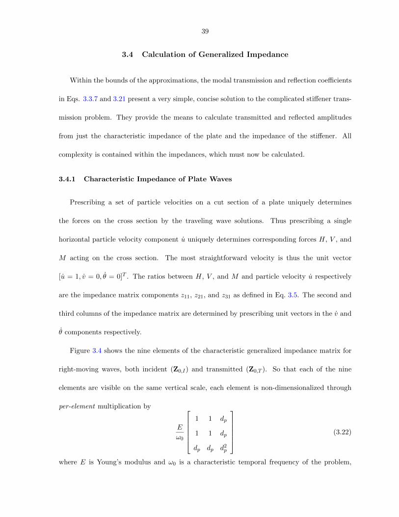
Figure 3.4 shows the nine elements of the characteristic generalized impedance matrix for
right-moving waves, both incident (Z0,I) and transmitted (Z0,T ). So that each of the nine
elements are visible on the same vertical scale, each element is non-dimensionalized through
per-element multiplication by
E
ω0
1 1 dp
1 1 dp
dp dp d2p
(3.22)
where E is Young’s modulus and ω0 is a characteristic temporal frequency of the problem,
40
0 50 100 150 200 250 300−4
−3
−2
−1
0
1
2
3
4
Hor
izon
talf
orce
,H
Horizontal velocity, u
0 50 100 150 200 250 300−4
−3
−2
−1
0
1
2
3
4Vertical velocity, v
0 50 100 150 200 250 300−4
−3
−2
−1
0
1
2
3
4Rotational velocity, θ
0 50 100 150 200 250 300−4
−3
−2
−1
0
1
2
3
4
Ver
tica
lfor
ce,V
0 50 100 150 200 250 300−4
−3
−2
−1
0
1
2
3
4
0 50 100 150 200 250 300−4
−3
−2
−1
0
1
2
3
4
0 50 100 150 200 250 300
Frequency, f , kHz
−4
−3
−2
−1
0
1
2
3
4
Mom
ent,M
0 50 100 150 200 250 300
Frequency, f , kHz
−4
−3
−2
−1
0
1
2
3
4
0 50 100 150 200 250 300
Frequency, f , kHz
−4
−3
−2
−1
0
1
2
3
4
Figure 3.4 The nine non-dimensionalized elements of the characteristic generalized impedance
of incident waves, shown with real part (- -), imaginary part (· · · ), and modulus
(—).
chosen arbitrarily to be 100kHz for this geometry and material. Four of the elements in Fig. 3.4
are identically zero. They are identically zero because horizontal force and particle velocity
correspond to symmetric Lamb waves, whereas vertical/rotational forces/particle velocities
correspond to antisymmetric Lamb waves. Since symmetric and antisymmetric Lamb waves
are decoupled the impedance matrix must also be decoupled.
Characteristic impedance for reflected waves (Z0,R) are calculated by the same procedure.
41
(0,0)
(0, )dp2
(0,ls+ )dp2
dp
ds
ls
x
y
B
J
E
Figure 3.5 Coordinate system for the stiffener cross-section.
Results are the same as Fig. 3.4 except the z2,3 and z3,2 elements are negated because of the
opposite propagation direction. For both right and left-moving waves, all of the impedance
components are slowly varying as a function of frequency.
3.4.2 Stiffener Impedance
The impedance of the stiffener is calculated in a similar manner. The stiffener, however,
has three extra constraints since there is no normal force, shear force, or moment acting on the
free end of the stiffener. Figure 3.5 shows the coordinate system for the impedance calculation.
The impedance if first calculated about the base of the stiffener, point B. To calculate the first
column of the impedance matrix, a particle velocity vector in the u direction is prescribed at
the base of the stiffener, the same as was done to calculate the characteristic impedance of the
plate. Since there are wave components traveling up and down the plate however, there are
six unknown wave amplitudes instead of the three wave amplitudes for waves travling a single
direction in a plate. This means three extra equations are needed to solve for the forces at
the base of the stiffener and calculate the impedance components. The three extra equations
42
come in the form of the stress-free condition at the free end of the stiffener. The equations
HS(y) = 0, VS(y) = 0, and MS(y) = 0 where HS(y), VS(y), and MS(y) are the traveling wave
solutions for the horizontal force, vertical force, and moment in the stiffener, are evaluated at
the free end of the stiffener. Together with the particle velocity equations at the base of the
stiffener, these six equations are solved using computer algebra. This determines the three force
components acting on the base of the stiffener, from which a single column of the impedance
matrix is calculated. As for the plate, unit particle velocities in the v and θ directions produce
the other two columns.
In this manner, the impedance ZS,B is first calculated about the base of the stiffener (point
B). We treat the stiffener as only the material above the surface of underlying plate and will
then extrapolate to determine an effective impedance at joint J , consistent with the forces at
point J defined in Fig. 3.2. This perturbed impedance accounts for rotation of the base of the
stiffener (point B) about the center of the junction (point J) due to the rotational component
of the wave, and also accounts for shear and longitudinal strain in the stiffener.
Fig. 3.5 shows a cross section of the stiffener-plate combination. The plate has thickness
dp, and the stiffener has width ds and height ls. The dashed lines (- -) indicate the cuts
that separate the domain into three regions: the incoming/reflected wave side to the left, the
transmitted wave side to the right, and the stiffener.
The base of the stiffener applies a force to point B. To connect this to the impedance
calculations of Eq. ??, we need to replace it by an equivalent force applied to the center of the
junction, point J . From the free body diagram, we consider the effect of force FS,B at point J
43
by writing
FS,J =
HB
VB
MB −HBdp2
=
1 0 0
0 1 0
−dp2 0 1
︸ ︷︷ ︸
K1
HB
VB
MB
, (3.23)
where the moment is decreased by the shear force HB times perpendicular distancedp2 . The
transformation can be represented as a matrix K1. In vector notation,
FS,J = K1FS,B. (3.24)
For small plate thicknesses, K1 approaches the identity matrix.
We state particle velocity uS,B in terms of uS,J by first observering that vertical offset at the
base of the stiffener leads to lateral motion when the plate rotates. In terms of displacements,
uS,B = uS,J −dp2
sin(θS,J) ≈ uS,J −dp2θS,J . (3.25)
Longitudinal strain in the stiffener causes vertical displacement of the base of the stiffener,
vS,B = vS,J −∂vS∂y
∣∣∣∣B
· dp2, (3.26)
and shear strain produces lateral displacement
uS,B = uS,J −∂uS∂y
∣∣∣∣B
· dp2. (3.27)
Approximate continuity of rotation throughout the junction implies, simply,
θS,B = θS,J . (3.28)
In matrix form, these modifications become
uS,B
vS,B
θS,B
=
uS,J
vS,J
θS,J
+
−dp
2 θS,J
0
0
+
−∂uS∂y
∣∣∣B
dp2
0
− ∂vS∂y
∣∣∣B
dp2
0
(3.29)
44
The first two vectors on the righthand side are easily combined by defining a perturbed identity
matrix K2 to yielduS,B
vS,B
θS,B
=
1 0 −dp
2
0 1 0
0 0 1
︸ ︷︷ ︸
K2
uS,J
vS,J
θS,J
+
−∂uS
∂y
∣∣∣B
dp2
−∂vS∂y
∣∣∣B
dp2
0
. (3.30)
Elimination of the last term follows from evaluation of the constituitive equation for normal
force in the stiffener at point B. Starting with the constituitive equation,
σyy = Eεyy, (3.31)
substitution of the parameters of this problem gives
VS,Bds
= E∂vS∂y
∣∣∣∣B
. (3.32)
In a similar manner, the shear stress is put in terms of forces and displacements. The shear
force is related to shear strain by
σxy = 2Gεxy. (3.33)
Similar substitution of forces and displacements gives
HS,B
ds= 2G
∂vS∂y
∣∣∣∣B
. (3.34)
Stated in terms of forces and differentiated in time, Eq. 3.30 becomes
uS,B = K2uS,J +
−iω dp
ds
HS,B
4G
−iω dpds
VS,B
2E
0
. (3.35)
Factorization again puts the equation in terms of known quantities, yielding
uS,B = K2uS,J +
−iω dp
ds14G 0 0
0 −iω dpds
12E 0
0 0 0
︸ ︷︷ ︸
K3
FS,B (3.36)
45
Generalized stiffener impedance about point J is defined by
FS,J = ZS,J uS,J . (3.37)
Substituting Eq. 3.36 into Eq. 3.37,
K−11 FS,J = ZS,B (K2uS,J +K3FS,B) , (3.38)
and rearranging yields the desired relation between FS,J and uS,J ,
FS,J =(I −K1ZS,BK3K
−11
)−1K1ZS,BK2︸ ︷︷ ︸
ZS,J
uS,J , (3.39)
FS,J = ZS,J uS,J , (3.40)
where I is the identity matrix and ZS,J is the resulting perturbed stiffener impedance matrix.
Note that as dp in K2 and K3 approaches zero, ZS,J approaches the unperturbed ZS,B.
Fig. 3.6 shows all nine elements of the stiffener impedance ZS,J , plotted as a function of
frequency and with the same normalization as for Fig. 3.4. The strictly imaginary impedances
indicate a purely reactive stiffener that transmits no net power into or out of the stiffener. The
most obvious difference compared to the characteristic impedance of the plate is the presence of
sharp peaks in all nonzero elements. These points of large impedance correspond to resonances
of the A0 or S0 modes traveling up and down in the stiffener. The ‘×’ shape of nonzero
elements in ZS,J reflects decoupling of vertical force/particle velocity from horizontal/rotational
forces/particle velocities. The interchange between horizontal and vertical between the plate
and stiffener switches which component is decoupled. It is this difference that drives the mode
conversion at low frequencies.
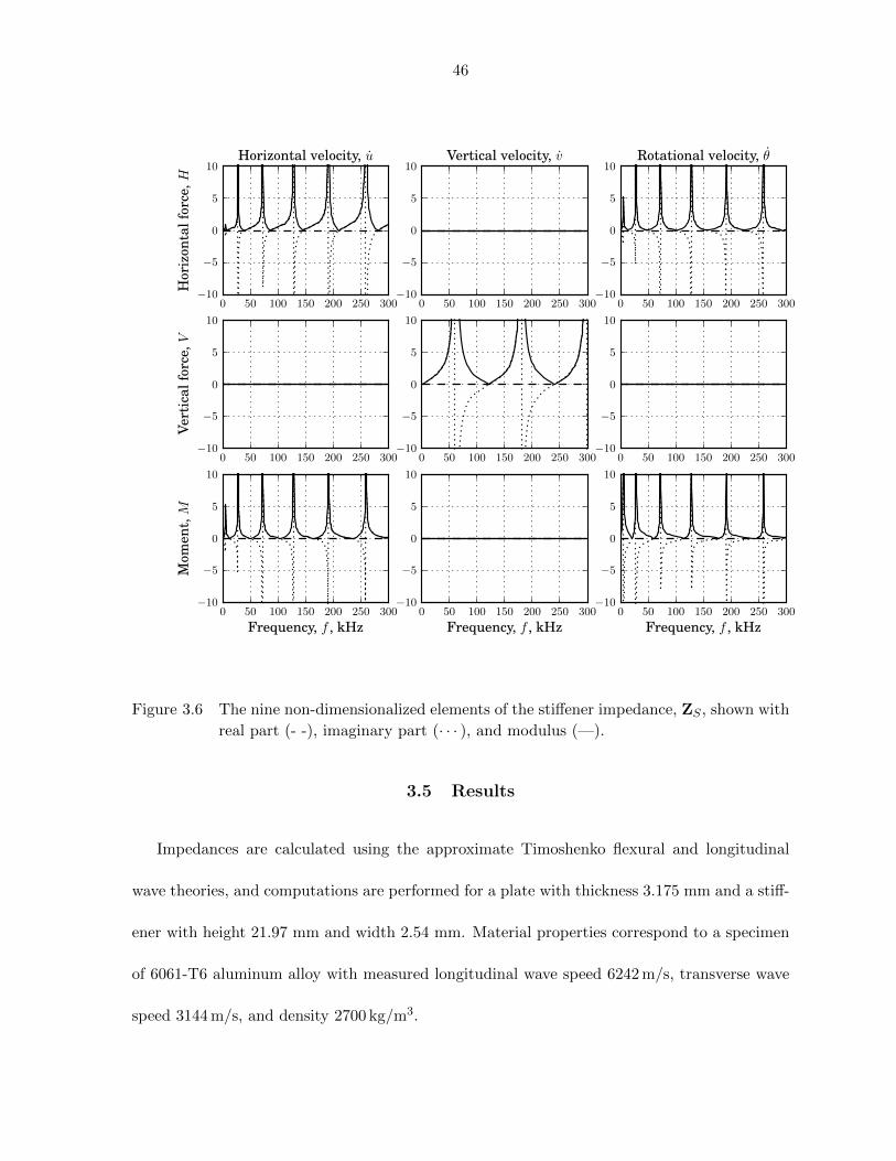
46
0 50 100 150 200 250 300−10
−5
0
5
10
Hor
izon
talf
orce
,H
Horizontal velocity, u
0 50 100 150 200 250 300−10
−5
0
5
10Vertical velocity, v
0 50 100 150 200 250 300−10
−5
0
5
10Rotational velocity, θ
0 50 100 150 200 250 300−10
−5
0
5
10
Ver
tica
lfor
ce,V
0 50 100 150 200 250 300−10
−5
0
5
10
0 50 100 150 200 250 300−10
−5
0
5
10
0 50 100 150 200 250 300
Frequency, f , kHz
−10
−5
0
5
10
Mom
ent,M
0 50 100 150 200 250 300
Frequency, f , kHz
−10
−5
0
5
10
0 50 100 150 200 250 300
Frequency, f , kHz
−10
−5
0
5
10
Figure 3.6 The nine non-dimensionalized elements of the stiffener impedance, ZS , shown with
real part (- -), imaginary part (· · · ), and modulus (—).
3.5 Results
Impedances are calculated using the approximate Timoshenko flexural and longitudinal
wave theories, and computations are performed for a plate with thickness 3.175 mm and a stiff-
ener with height 21.97 mm and width 2.54 mm. Material properties correspond to a specimen
of 6061-T6 aluminum alloy with measured longitudinal wave speed 6242 m/s, transverse wave
speed 3144 m/s, and density 2700 kg/m3.
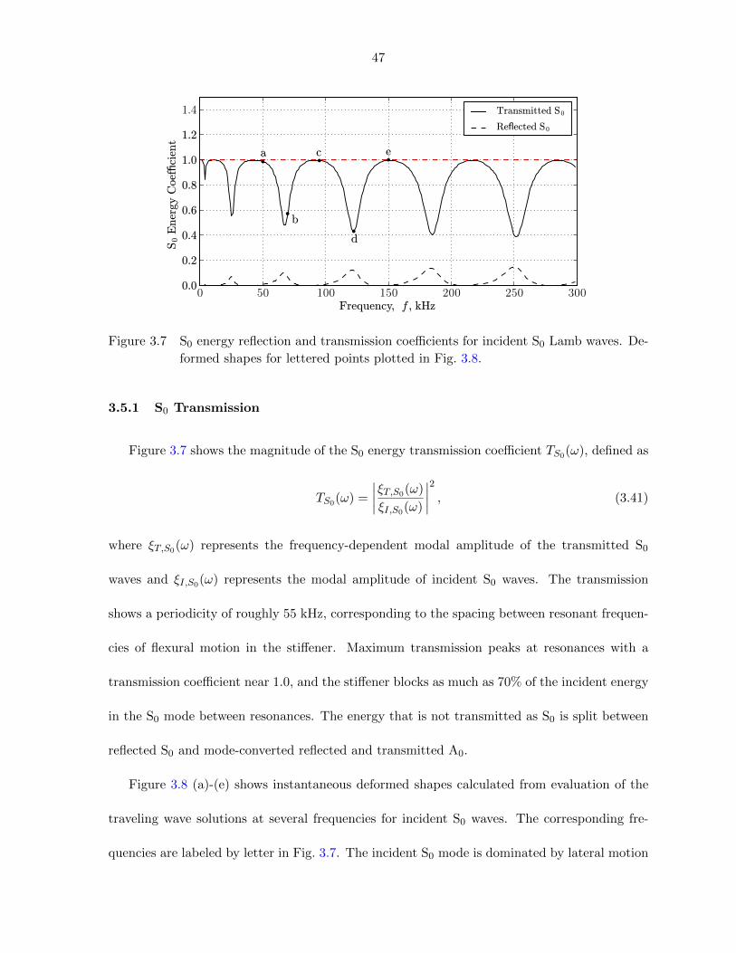
47
0 50 100 150 200 250 300Frequency, f , kHz
0.0
0.2
0.4
0.6
0.8
1.0
1.2
1.4
S0EnergyCoefficient
Transmitted S0
Reflected S0
b
c
d
ea
Figure 3.7 S0 energy reflection and transmission coefficients for incident S0 Lamb waves. De-
formed shapes for lettered points plotted in Fig. 3.8.
3.5.1 S0 Transmission
Figure 3.7 shows the magnitude of the S0 energy transmission coefficient TS0(ω), defined as
TS0(ω) =
∣∣∣∣ξT,S0(ω)
ξI,S0(ω)
∣∣∣∣2 , (3.41)
where ξT,S0(ω) represents the frequency-dependent modal amplitude of the transmitted S0
waves and ξI,S0(ω) represents the modal amplitude of incident S0 waves. The transmission
shows a periodicity of roughly 55 kHz, corresponding to the spacing between resonant frequen-
cies of flexural motion in the stiffener. Maximum transmission peaks at resonances with a
transmission coefficient near 1.0, and the stiffener blocks as much as 70% of the incident energy
in the S0 mode between resonances. The energy that is not transmitted as S0 is split between
reflected S0 and mode-converted reflected and transmitted A0.
Figure 3.8 (a)-(e) shows instantaneous deformed shapes calculated from evaluation of the
traveling wave solutions at several frequencies for incident S0 waves. The corresponding fre-
quencies are labeled by letter in Fig. 3.7. The incident S0 mode is dominated by lateral motion
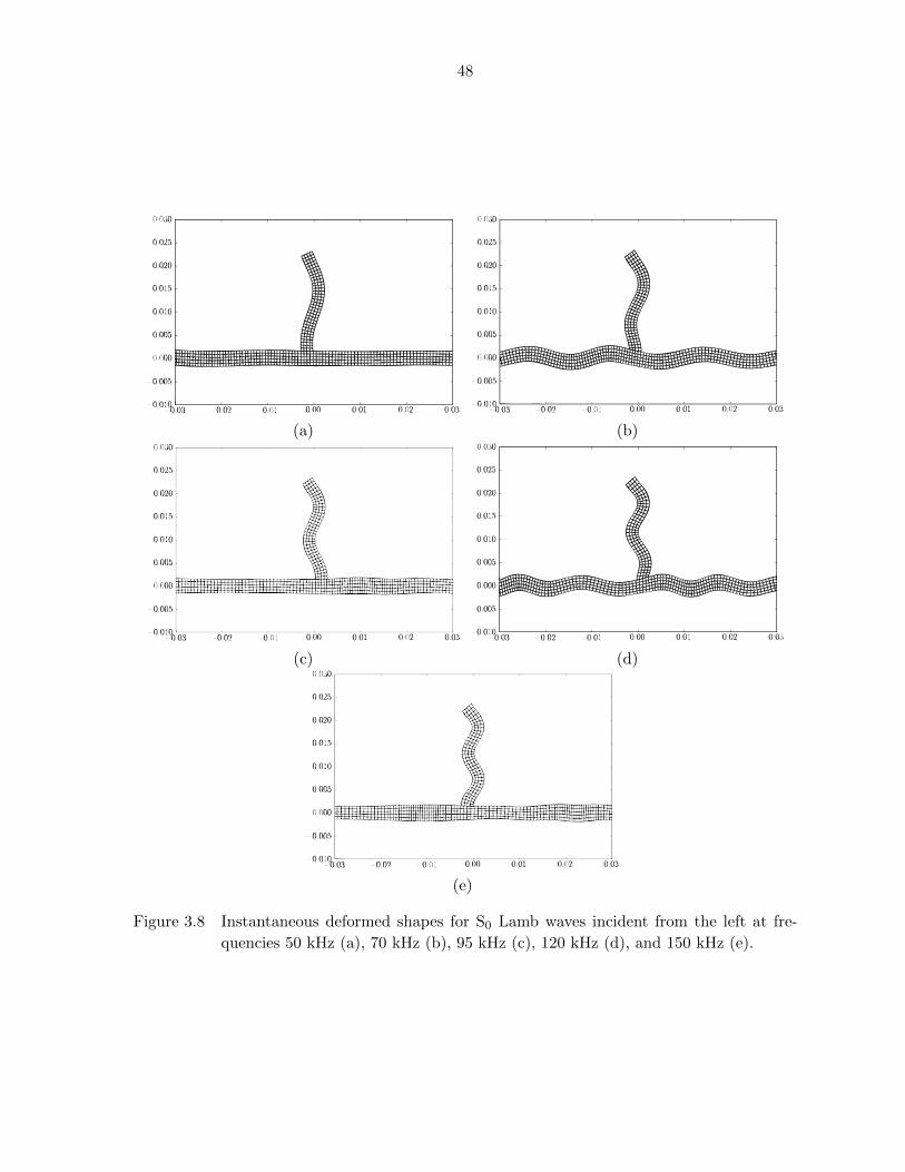
48
(a) (b)
(c) (d)
(e)
Figure 3.8 Instantaneous deformed shapes for S0 Lamb waves incident from the left at fre-
quencies 50 kHz (a), 70 kHz (b), 95 kHz (c), 120 kHz (d), and 150 kHz (e).
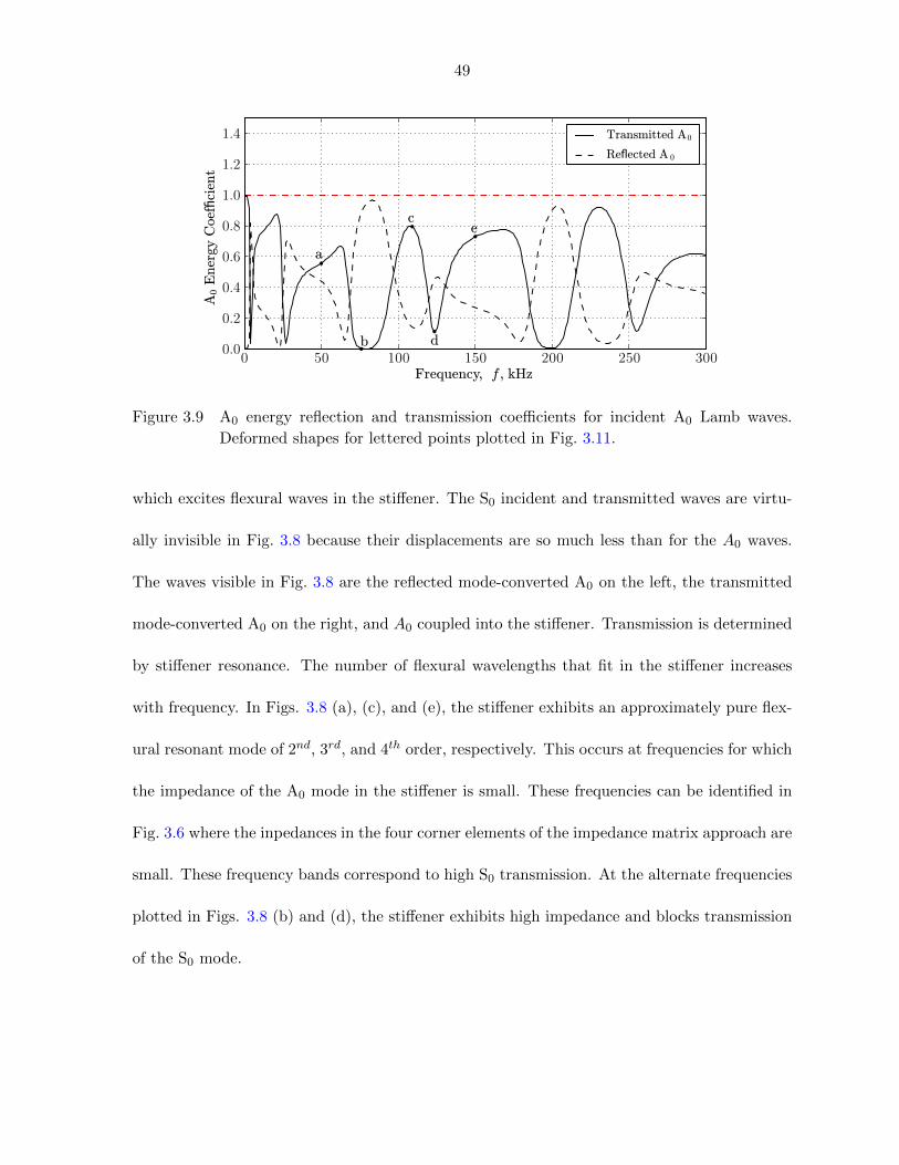
49
0 50 100 150 200 250 300Frequency, f , kHz
0.0
0.2
0.4
0.6
0.8
1.0
1.2
1.4
A0EnergyCoefficient
Transmitted A0
Reflected A 0
a
b
c
d
e
Figure 3.9 A0 energy reflection and transmission coefficients for incident A0 Lamb waves.
Deformed shapes for lettered points plotted in Fig. 3.11.
which excites flexural waves in the stiffener. The S0 incident and transmitted waves are virtu-
ally invisible in Fig. 3.8 because their displacements are so much less than for the A0 waves.
The waves visible in Fig. 3.8 are the reflected mode-converted A0 on the left, the transmitted
mode-converted A0 on the right, and A0 coupled into the stiffener. Transmission is determined
by stiffener resonance. The number of flexural wavelengths that fit in the stiffener increases
with frequency. In Figs. 3.8 (a), (c), and (e), the stiffener exhibits an approximately pure flex-
ural resonant mode of 2nd, 3rd, and 4th order, respectively. This occurs at frequencies for which
the impedance of the A0 mode in the stiffener is small. These frequencies can be identified in
Fig. 3.6 where the inpedances in the four corner elements of the impedance matrix approach are
small. These frequency bands correspond to high S0 transmission. At the alternate frequencies
plotted in Figs. 3.8 (b) and (d), the stiffener exhibits high impedance and blocks transmission
of the S0 mode.
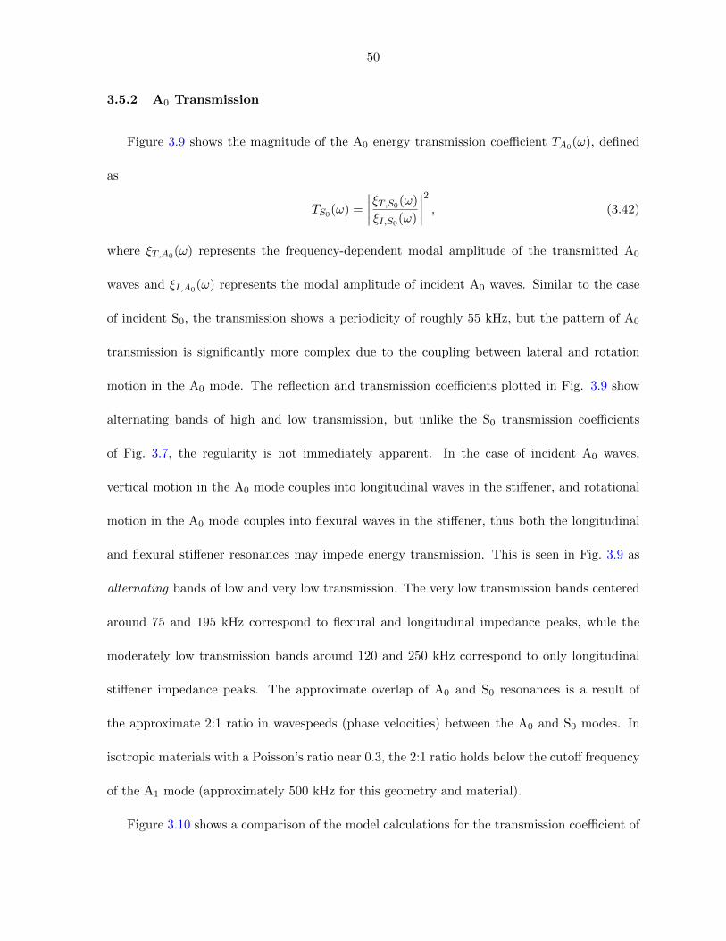
50
3.5.2 A0 Transmission
Figure 3.9 shows the magnitude of the A0 energy transmission coefficient TA0(ω), defined
as
TS0(ω) =
∣∣∣∣ξT,S0(ω)
ξI,S0(ω)
∣∣∣∣2 , (3.42)
where ξT,A0(ω) represents the frequency-dependent modal amplitude of the transmitted A0
waves and ξI,A0(ω) represents the modal amplitude of incident A0 waves. Similar to the case
of incident S0, the transmission shows a periodicity of roughly 55 kHz, but the pattern of A0
transmission is significantly more complex due to the coupling between lateral and rotation
motion in the A0 mode. The reflection and transmission coefficients plotted in Fig. 3.9 show
alternating bands of high and low transmission, but unlike the S0 transmission coefficients
of Fig. 3.7, the regularity is not immediately apparent. In the case of incident A0 waves,
vertical motion in the A0 mode couples into longitudinal waves in the stiffener, and rotational
motion in the A0 mode couples into flexural waves in the stiffener, thus both the longitudinal
and flexural stiffener resonances may impede energy transmission. This is seen in Fig. 3.9 as
alternating bands of low and very low transmission. The very low transmission bands centered
around 75 and 195 kHz correspond to flexural and longitudinal impedance peaks, while the
moderately low transmission bands around 120 and 250 kHz correspond to only longitudinal
stiffener impedance peaks. The approximate overlap of A0 and S0 resonances is a result of
the approximate 2:1 ratio in wavespeeds (phase velocities) between the A0 and S0 modes. In
isotropic materials with a Poisson’s ratio near 0.3, the 2:1 ratio holds below the cutoff frequency
of the A1 mode (approximately 500 kHz for this geometry and material).
Figure 3.10 shows a comparison of the model calculations for the transmission coefficient of
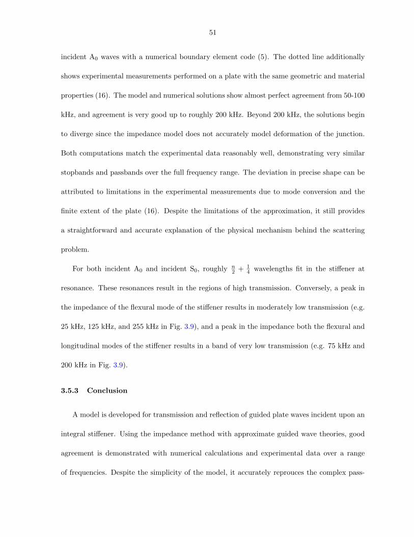
51
incident A0 waves with a numerical boundary element code (5). The dotted line additionally
shows experimental measurements performed on a plate with the same geometric and material
properties (16). The model and numerical solutions show almost perfect agreement from 50-100
kHz, and agreement is very good up to roughly 200 kHz. Beyond 200 kHz, the solutions begin
to diverge since the impedance model does not accurately model deformation of the junction.
Both computations match the experimental data reasonably well, demonstrating very similar
stopbands and passbands over the full frequency range. The deviation in precise shape can be
attributed to limitations in the experimental measurements due to mode conversion and the
finite extent of the plate (16). Despite the limitations of the approximation, it still provides
a straightforward and accurate explanation of the physical mechanism behind the scattering
problem.
For both incident A0 and incident S0, roughly n2 + 1
4 wavelengths fit in the stiffener at
resonance. These resonances result in the regions of high transmission. Conversely, a peak in
the impedance of the flexural mode of the stiffener results in moderately low transmission (e.g.
25 kHz, 125 kHz, and 255 kHz in Fig. 3.9), and a peak in the impedance both the flexural and
longitudinal modes of the stiffener results in a band of very low transmission (e.g. 75 kHz and
200 kHz in Fig. 3.9).
3.5.3 Conclusion
A model is developed for transmission and reflection of guided plate waves incident upon an
integral stiffener. Using the impedance method with approximate guided wave theories, good
agreement is demonstrated with numerical calculations and experimental data over a range
of frequencies. Despite the simplicity of the model, it accurately reprouces the complex pass-
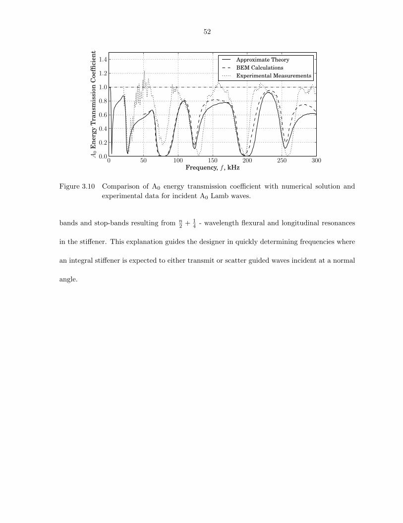
52
0 50 100 150 200 250 300Frequency, f , kHz
0.0
0.2
0.4
0.6
0.8
1.0
1.2
1.4
A0
Ene
rgy
Tran
smis
sion
Coe
ffici
ent
Approximate TheoryBEM CalculationsExperimental Measurements
Figure 3.10 Comparison of A0 energy transmission coefficient with numerical solution and
experimental data for incident A0 Lamb waves.
bands and stop-bands resulting from n2 + 1
4 - wavelength flexural and longitudinal resonances
in the stiffener. This explanation guides the designer in quickly determining frequencies where
an integral stiffener is expected to either transmit or scatter guided waves incident at a normal
angle.
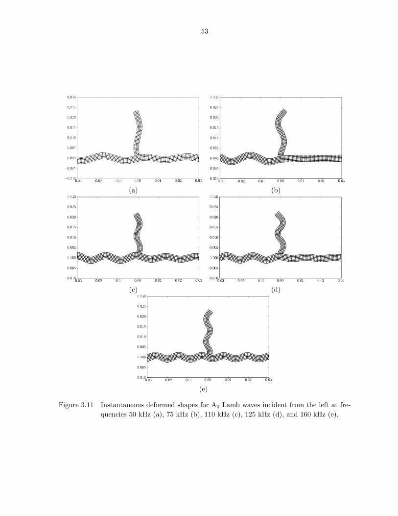
53
(a) (b)
(c) (d)
(e)
Figure 3.11 Instantaneous deformed shapes for A0 Lamb waves incident from the left at fre-
quencies 50 kHz (a), 75 kHz (b), 110 kHz (c), 125 kHz (d), and 160 kHz (e).
54
Bibliography
[1] A. Raghavan, C. E. S. Cesnik, “Review of Guided-wave Structural Health Monitoring,”
The Shock and Vibration Digest 39(2), pp. 91-114, (2007).
[2] A. Cheng, D. Cheng, “Heritage and early history of the boundary element method,”
Engineering Analysis with Boundary Elements 29, pp. 268-302, (2005).
[3] J. D. Achenbach, Reciprocity in Elastodynamics, (Cambridge Univ Press, London, 2003).
[4] R. A. Roberts, “Guided wave propagation in integrally stiffened plates,” in Review of
Progress in Quantitative Nondestructive Evaluation, vol. 27, D. O. Thompson, D. E.
Chimenti, Eds. (AIP Press, New York, 2008), pp. 170–177.
[5] R. A. Roberts, “Plate wave transmission/reflection at geometric obstructions: model
study,” Review of Progress in Quantitative Nondestructive Evaluation, vol. 29, D. O.
Thompson, D. E. Chimenti, Eds. (AIP Press, New York, 2010), pp. 192–199.
[6] P. Wilcox, A. Velichko, B. Drinkwater, A. Croxford, “Scattering of plane guided waves
obliquely incident on a straight feature with uniform cross-section,” J. Acoust. Soc. Am.
128(5), pp. 2715-2725, (2010).
[7] J. P. Lee, H. Kolsky, “The Generation of Stress Pulses at the Junction of Two Noncollinear
Rods,” Journal of Applied Mechanics 39(3), pp. 809-814, (1972).

55
[8] K. J. Yong, K. J. Atkins, “Generation of elastic stress waves at a T-junction of square
rods,” Journal of Sound and Vibration 88(4), pp. 431-436, (1983).
[9] J. D. Achenbach, Wave propagation in elastic solids, American Elselvier, (1973).
[10] Y. Cho, J. Rose, “A boundary element solution for a mode conversion study on the edge
reflection of Lamb waves,” Journal of the Acoustical Society of America, 99(4), pp. 2097-
2109, (1996).
[11] B. Morvan, N. Wilie-Chancellier, H. Duflo, A. Tinel, J. Duclos, “Lamb wave reflection at
the free edge of a plate” in J. Acoust. Soc. Am. 113(3), pp. 1417-1425, (2003).
[12] S. A. Martin, K. V. Jata, “FEM modeling of guided wave behavior in integrally stiffened
plate structures,” SPIE Proceedings, Vol. 6529, (2007).
[13] D. W. Greve, N. Tyson, I. J. Oppenheim, “Interaction of defects with Lamb waves in
complex geometries,” IEEE Ultrasonics Conference Proceedings, 297-300, (2005).
[14] W. C. Elmore, M. A. Heald, Physics of Waves, Dover Publications, (1985).
[15] K. Graff, Wave Motion in Elastic Solids, Dover Publications, (1991).
[16] R.S. Reusser, D.E. Chimenti, R.A. Roberts, S.D. Holland, “Guided plate wave scattering
at vertical stiffeners and its effect on source location,” ULTRASONICS, In Press, Accepted
for Publication 26 October 2011.
56
CHAPTER 4. Conclusions
4.1 Summary
The case of waves normally incident upon an integral stiffener has been studied in detail
and the results have been applied to the problem of spacecraft leak location.
In the first part of this work, transmission of the A0 guided wave mode normally incident
upon a low and high aspect ratio stiffener is measured and related to performance of a leak
location system for manned spacecraft. A pattern of high and low transmission frequency
bands is observed. It is demonstrated that integral stiffeners acting as frequency-dependent
filters limit the range of the leak location system. Although normal incidence upon a stiffener
does not adequately describe guided wave interaction with the complex pattern of stiffeners,
very good correlation is observed between normal transmission and the ability of a virtual
detector to locate a synthetic leak source. Based on these observations, two algorithms are
proposed for determing the best frequency band for detecting leak-generated noise. The first,
termed in-situ calibration relies on virtual leak sources to determine a posteriori which narrow
frequency bands produce acceptable results. The second, termed wide bandwidth calibration,
simply uses all available frequencies. Wide bandwidth is determined to be the most robust
option since most stiffeners have rapidly varying transmission peaks and valleys and so will not
have a narrow frequency band that produces consistently acceptable results.
In the second part of this work, the mechanics of transmission past an integral stiffener at
57
normal incidence are examined in greater depth. Using approximate longitudinal and flexural
wave theories, a model is developed that accurately predicts low-frequency transmission and
reflection. For incident S0 waves, it is found that high transmission corresponds to low stiffener
mechanical impedance of flexural waves in the stiffener. Transmission of incident A0 waves is
found to depend on both the flexural and longitudinal resonances in the stiffener.
4.2 Recommendations for future research
Waves incident on a stiffener at an oblique angle have not been considered in this work.
The relatively simple mechanics governing the problem of normal incidence suggest that a
straightforward extrapolation is possible for angles of incidence close to normal. Wilcox (6)
takes a detailed look at computational methods and physical mechanisms for waves obliquely
incident on an adhesively bonded hollow square stiffener. The complexity of that problem
means it requires numerical solution, but it should be possible to gain a deeper understanding
of the somewhat simpler problem of waves obliquely incident on the integral stiffener considered
in this work. This would be invaluable information for the designer who desires approximate
guidelines rather than tabulated solutions for each possible case.
58
APPENDIX A. APPROXIMATE GUIDED WAVE THEORY
Timoshenko flexural wave approximation
The Timoshenko beam theory approximation (15) applied to flexural waves in a plate
captures the two lowest order flexural Lamb modes, the A0 and A1 modes. By accounting
for the rotation of the cross-section, Timoshenko derives a theory that, while still quasi one-
dimensional, closely approximates the exact Lamb wave solution.
A single traveling wave represents the solution, but the theory considers translation and
rotation separately. Transverse displacement v is represented by
v = B1ei(kx−ωt), (A.1)
where ei(kx−ωt) represents the traveling wave with wavenumber k and angular temporal fre-
quency ω, and B1 is an arbitrary coefficient defining the amplitude and phase of the wave.
The key feature of Timoshenko flexural wave theory is that a second traveling wave defines the
rotation ψ of the cross section plane, as opposed to the slope of the surface of the beam, ∂v∂x . ψ
is defined as
ψ = B2ei(kx−ωt), (A.2)
and it is related to the traveling wave solution for v by the relation
B2
B1= i
(Gκk2 − ρω2)
Gκk. (A.3)
59
Here, κ is the so-called shear coefficient, given as 0.833 for rectangular cross-sections. ρ is the
density of the material, and G is the shear modulus. Note that as ω → 0, B2B1→ ik, or a simple
derivative. Correspondingly, Timoshenko defines the moment and shear forces per depth acting
on a cross section of the plate as
M = −EI ∂ψ∂x
(A.4)
and
V =∂M
∂x+ ρI
∂2ψ
∂t2. (A.5)
From page 184 of Graff (15), the dispersion relation for these waves is
EI
ρAk4 − I
A
(1 +
E
Gκ
)k2ω2 − ω2 +
ρI
GAκω4 = 0, (A.6)
where κ is the so-called shear coefficient, with a value of 0.833 given for rectangular beam
cross-sections, and A is the area of the cross-section. This theory applies to plates as well as
beams since a plate is equivalent to a beam where everything has been scaled to unit depth.
Fig. 3.3 shows the result of Timoshenko’s approximation. Since Eq. A.6 is a fourth-order
polynomial in k, there are four corresponding roots. Two pairs differing only in sign correspond
to solutions oriented in opposite directions. For each pair, one root corresponds to the the lowest
order antisymmetric Lamb mode, A0, while the other corresponds to the second lowest order
antisymmetric Lamb mode, A1. At low frequencies, the branch corresponding to the A1 mode
is purely complex, indicating a non-propagating mode. Fig. 3.3 shows one pair of roots with
purely real wavenumbers in the right half-plane and purely imaginary wavenumbers in the left
half-plane.
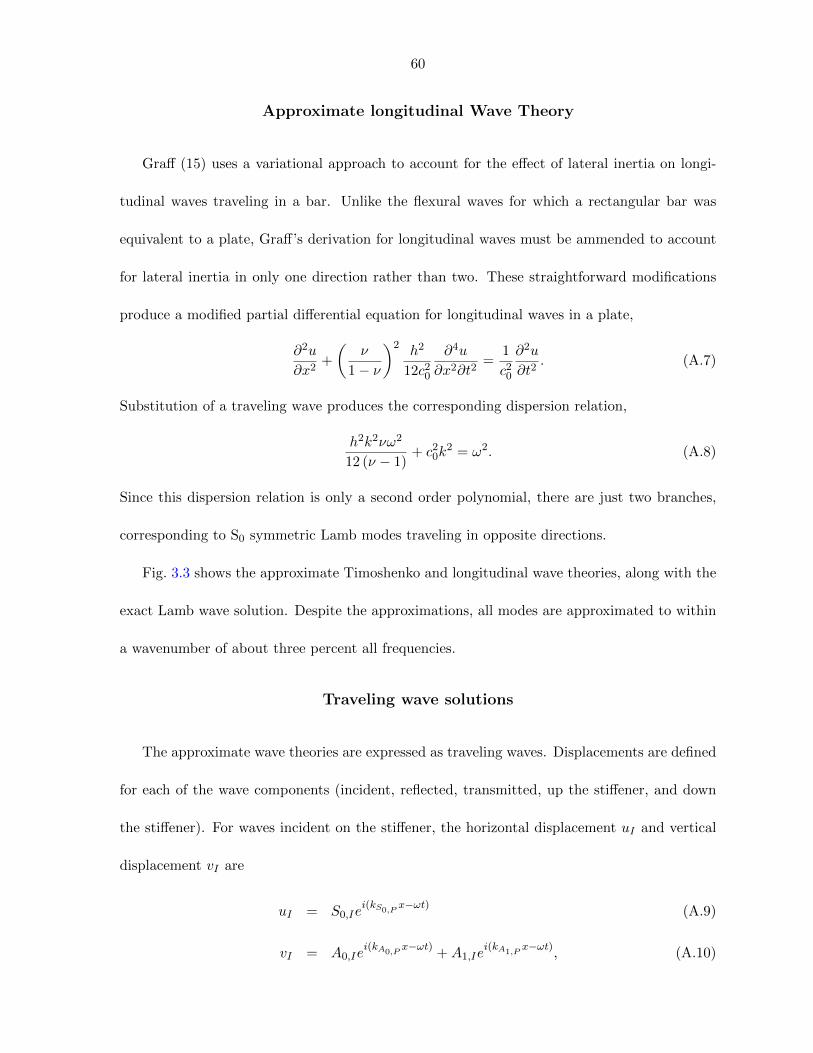
60
Approximate longitudinal Wave Theory
Graff (15) uses a variational approach to account for the effect of lateral inertia on longi-
tudinal waves traveling in a bar. Unlike the flexural waves for which a rectangular bar was
equivalent to a plate, Graff’s derivation for longitudinal waves must be ammended to account
for lateral inertia in only one direction rather than two. These straightforward modifications
produce a modified partial differential equation for longitudinal waves in a plate,
∂2u
∂x2+
(ν
1− ν
)2 h2
12c20
∂4u
∂x2∂t2=
1
c20
∂2u
∂t2. (A.7)
Substitution of a traveling wave produces the corresponding dispersion relation,
h2k2νω2
12 (ν − 1)+ c20k
2 = ω2. (A.8)
Since this dispersion relation is only a second order polynomial, there are just two branches,
corresponding to S0 symmetric Lamb modes traveling in opposite directions.
Fig. 3.3 shows the approximate Timoshenko and longitudinal wave theories, along with the
exact Lamb wave solution. Despite the approximations, all modes are approximated to within
a wavenumber of about three percent all frequencies.
Traveling wave solutions
The approximate wave theories are expressed as traveling waves. Displacements are defined
for each of the wave components (incident, reflected, transmitted, up the stiffener, and down
the stiffener). For waves incident on the stiffener, the horizontal displacement uI and vertical
displacement vI are
uI = S0,Iei(kS0,P
x−ωt)(A.9)
vI = A0,Iei(kA0,P
x−ωt)+A1,Ie
i(kA1,Px−ωt)
, (A.10)
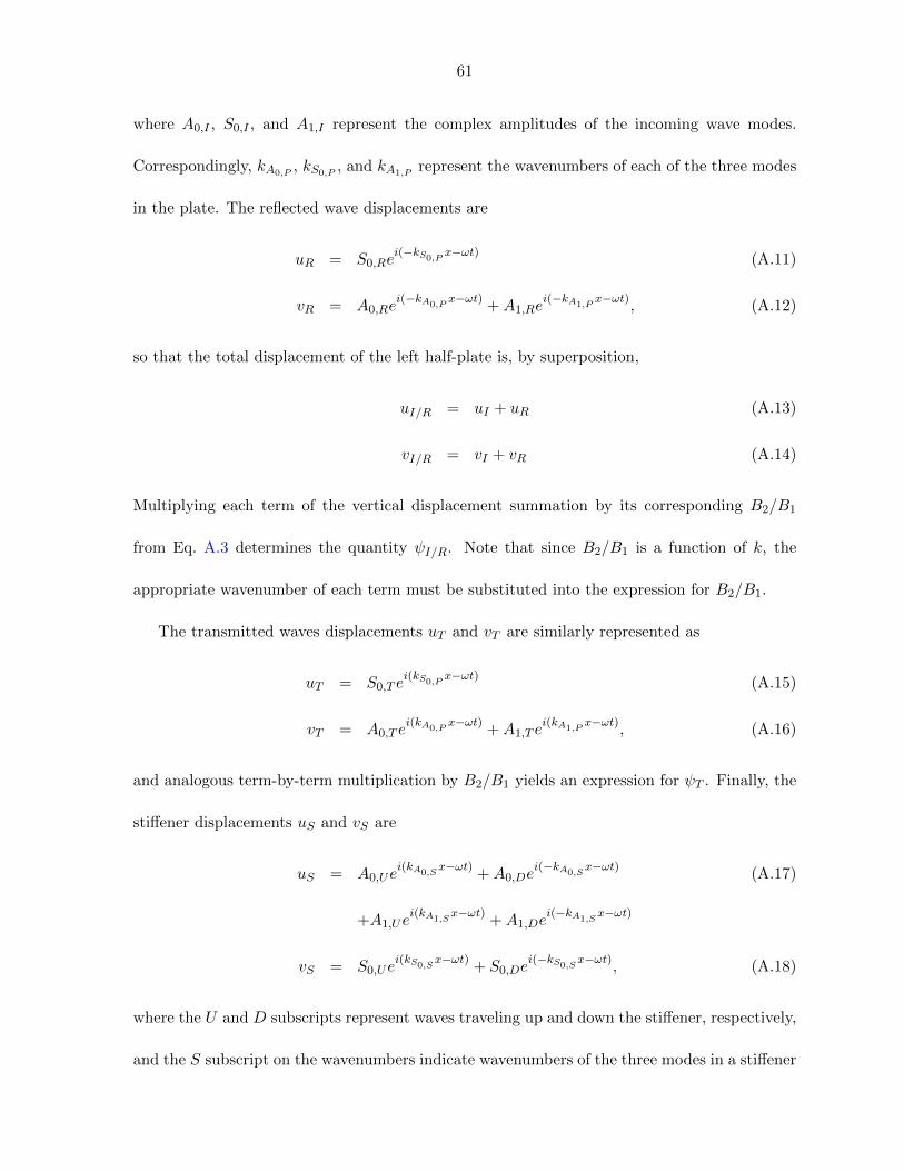
61
where A0,I , S0,I , and A1,I represent the complex amplitudes of the incoming wave modes.
Correspondingly, kA0,P, kS0,P
, and kA1,Prepresent the wavenumbers of each of the three modes
in the plate. The reflected wave displacements are
uR = S0,Rei(−kS0,P
x−ωt)(A.11)
vR = A0,Rei(−kA0,P
x−ωt)+A1,Re
i(−kA1,Px−ωt)
, (A.12)
so that the total displacement of the left half-plate is, by superposition,
uI/R = uI + uR (A.13)
vI/R = vI + vR (A.14)
Multiplying each term of the vertical displacement summation by its corresponding B2/B1
from Eq. A.3 determines the quantity ψI/R. Note that since B2/B1 is a function of k, the
appropriate wavenumber of each term must be substituted into the expression for B2/B1.
The transmitted waves displacements uT and vT are similarly represented as
uT = S0,T ei(kS0,P
x−ωt)(A.15)
vT = A0,T ei(kA0,P
x−ωt)+A1,T e
i(kA1,Px−ωt)
, (A.16)
and analogous term-by-term multiplication by B2/B1 yields an expression for ψT . Finally, the
stiffener displacements uS and vS are
uS = A0,Uei(kA0,S
x−ωt)+A0,De
i(−kA0,Sx−ωt)
(A.17)
+A1,Uei(kA1,S
x−ωt)+A1,De
i(−kA1,Sx−ωt)
vS = S0,Uei(kS0,S
x−ωt)+ S0,De
i(−kS0,Sx−ωt)
, (A.18)
where the U and D subscripts represent waves traveling up and down the stiffener, respectively,
and the S subscript on the wavenumbers indicate wavenumbers of the three modes in a stiffener
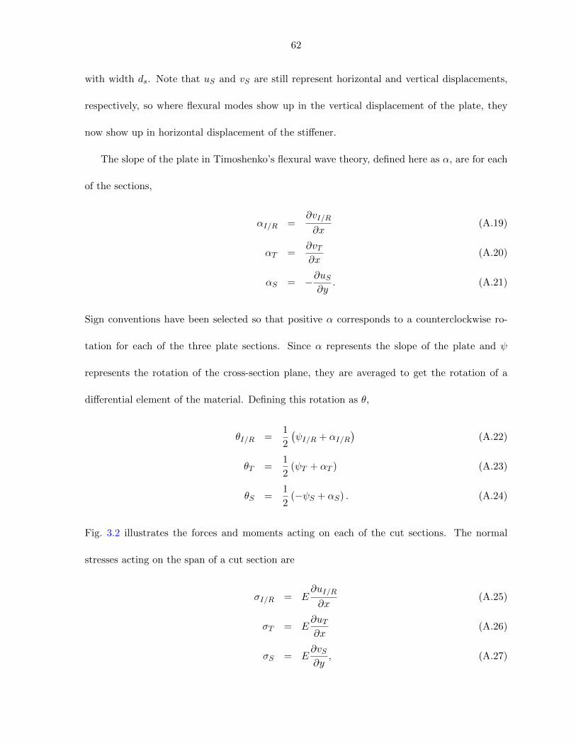
62
with width ds. Note that uS and vS are still represent horizontal and vertical displacements,
respectively, so where flexural modes show up in the vertical displacement of the plate, they
now show up in horizontal displacement of the stiffener.
The slope of the plate in Timoshenko’s flexural wave theory, defined here as α, are for each
of the sections,
αI/R =∂vI/R
∂x(A.19)
αT =∂vT∂x
(A.20)
αS = −∂uS∂y
. (A.21)
Sign conventions have been selected so that positive α corresponds to a counterclockwise ro-
tation for each of the three plate sections. Since α represents the slope of the plate and ψ
represents the rotation of the cross-section plane, they are averaged to get the rotation of a
differential element of the material. Defining this rotation as θ,
θI/R =1
2
(ψI/R + αI/R
)(A.22)
θT =1
2(ψT + αT ) (A.23)
θS =1
2(−ψS + αS) . (A.24)
Fig. 3.2 illustrates the forces and moments acting on each of the cut sections. The normal
stresses acting on the span of a cut section are
σI/R = E∂uI/R
∂x(A.25)
σT = E∂uT∂x
(A.26)
σS = E∂vS∂y
, (A.27)
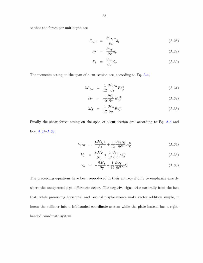
63
so that the forces per unit depth are
FI/R =∂uI/R
∂xdp (A.28)
FT =∂uT∂x
dp (A.29)
FS =∂vS∂y
ds. (A.30)
The moments acting on the span of a cut section are, according to Eq. A.4,
MI/R =1
12
∂ψI/R
∂xEd3p (A.31)
MT =1
12
∂ψT
∂xEd3p (A.32)
MS =1
12
∂ψS
∂yEd3s (A.33)
Finally the shear forces acting on the span of a cut section are, according to Eq. A.5 and
Eqs. A.31–A.33,
VI/R =∂MI/R
∂x+
1
12
∂ψI/R
∂t2ρd3p (A.34)
VT =∂MT
∂x+
1
12
∂ψT
∂t2ρd3p (A.35)
VS = −∂MS
∂y+
1
12
∂ψS
∂t2ρd3s (A.36)
The preceeding equations have been reproduced in their entirety if only to emphasize exactly
where the unexpected sign differences occur. The negative signs arise naturally from the fact
that, while preserving horizontal and vertical displacements make vector addition simple, it
forces the stiffener into a left-handed coordinate system while the plate instead has a right-
handed coordinate system.
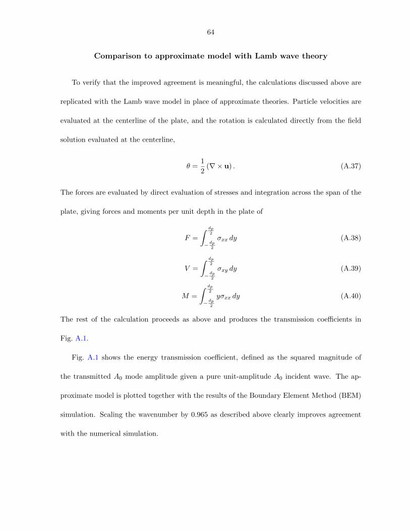
64
Comparison to approximate model with Lamb wave theory
To verify that the improved agreement is meaningful, the calculations discussed above are
replicated with the Lamb wave model in place of approximate theories. Particle velocities are
evaluated at the centerline of the plate, and the rotation is calculated directly from the field
solution evaluated at the centerline,
θ =1
2(∇× u) . (A.37)
The forces are evaluated by direct evaluation of stresses and integration across the span of the
plate, giving forces and moments per unit depth in the plate of
F =
∫ dp2
− dp2
σxx dy (A.38)
V =
∫ dp2
− dp2
σxy dy (A.39)
M =
∫ dp2
− dp2
yσxx dy (A.40)
The rest of the calculation proceeds as above and produces the transmission coefficients in
Fig. A.1.
Fig. A.1 shows the energy transmission coefficient, defined as the squared magnitude of
the transmitted A0 mode amplitude given a pure unit-amplitude A0 incident wave. The ap-
proximate model is plotted together with the results of the Boundary Element Method (BEM)
simulation. Scaling the wavenumber by 0.965 as described above clearly improves agreement
with the numerical simulation.
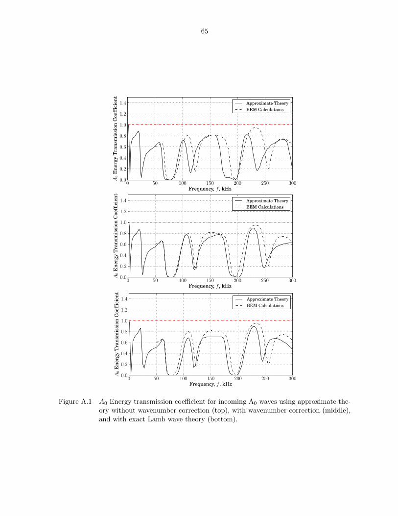
65
0 50 100 150 200 250 300Frequency, f , kHz
0.0
0.2
0.4
0.6
0.8
1.0
1.2
1.4
A0
Ene
rgy
Tran
smis
sion
Coe
ffici
ent
Approximate TheoryBEM Calculations
0 50 100 150 200 250 300Frequency, f , kHz
0.0
0.2
0.4
0.6
0.8
1.0
1.2
1.4
A0
Ene
rgy
Tran
smis
sion
Coe
ffici
ent
Approximate TheoryBEM Calculations
0 50 100 150 200 250 300Frequency, f , kHz
0.0
0.2
0.4
0.6
0.8
1.0
1.2
1.4
A0
Ene
rgy
Tran
smis
sion
Coe
ffici
ent
Approximate TheoryBEM Calculations
Figure A.1 A0 Energy transmission coefficient for incoming A0 waves using approximate the-ory without wavenumber correction (top), with wavenumber correction (middle),and with exact Lamb wave theory (bottom).