Boundary integral methods in high frequency scattering

Book or Report Section

Accepted Version

Postprint version (accepted for publication)

Chandler-Wilde, S. N. and Graham, I. G. (2009) Boundary integral methods in high frequency scattering. In: Engquist, B., Fokas, T., Hairer, E. and Iserles, A. (eds.) Highly Oscillatory Problems. London Mathematical Society Lecture Note Series (366). Cambridge University Press, Cambridge, pp. 154-193. ISBN 9780521134439 Available at http://centaur.reading.ac.uk/1584/

It is advisable to refer to the publisher’s version if you intend to cite from the work. See Guidance on citing .Published version at: http://www.cambridge.org/uk/catalogue/catalogue.asp?isbn=9780521134439

Publisher: Cambridge University Press

All outputs in CentAUR are protected by Intellectual Property Rights law, including copyright law. Copyright and IPR is retained by the creators or other copyright holders. Terms and conditions for use of this material are defined in the End User Agreement .

www.reading.ac.uk/centaur

CentAUR

Central Archive at the University of Reading

Reading’s research outputs online

Boundary integral methods in high frequency scattering

Simon N. Chandler-Wilde ∗ Ivan G. Graham†

Abstract

In this article we review recent progress on the design, analysis and implementation

of numerical-asymptotic boundary integral methods for the computation of frequency-

domain acoustic scattering in a homogeneous unbounded medium by a bounded obstacle.

The main aim of the methods is to allow computation of scattering at arbitrarily high

frequency with finite computational resources.

1 Introduction

There is huge mathematical and engineering interest in acoustic and electromagnetic wavescattering problems, driven by many applications such as modelling radar, sonar, acous-tic noise barriers, atmospheric particle scattering, ultrasound and VLSI. For time harmonicproblems in infinite domains and media which are predominantly homogeneous, the boundaryelement method is a very popular solver, used in a number of large commercial codes, see e.g.[26]. In many practical applications the characteristic length scale L of the domain is largecompared to the wavelength λ. Then the small dimensionless wavelength λ/L induces oscilla-tory solutions, and the application of conventional (piecewise polynomial) boundary elementsfor this multiscale problem yields full matrices of dimension at least N = (L/λ)d−1 (in R

d).(Domain finite elements lead to sparse matrices but require even larger N .) Since this “loss ofrobustness” as L/λ → ∞ puts high frequency problems outside the reach of many standardalgorithms, much recent research has been devoted to finding more robust methods.

One approach is to seek faster implementations of standard methods. Fast multipole meth-ods have allowed conventional BEM solutions for much larger N (e.g. [28, 29]), but it remainsimpossible to compute with L/λ much beyond a few hundred in 3D. To allow larger L/λ, ahighly promising new direction is the development of “hybrid” algorithms, which incorporateasymptotic information about the oscillation of the solution into the approximation space[1, 2, 12, 38, 50, 22, 59, 6, 23, 30, 13, 32, 43]. Initial experiments using geometric-opticstype approximations on simple model problems indicate the possibility of delivering almost

∗Department of Mathematics, University of Reading, P.O.Box 220, Whiteknights, RG6 6AX, U.K.

S.N.Chandler-Wilde@reading.ac.uk†Department of Mathematical Sciences, University of Bath, Bath BA2 7AY, UK. I.G.Graham@bath.ac.uk

1

uniform accuracy for N fixed as L/λ → ∞. This review will explain the key ideas behindthese methods and the mathematical tools which have been so-far developed for their analysis.We also highlight some important open problems which are the focus of current research inthis very active area. Another approach to high frequency problems, involving the solution ofappropriate limiting problems, is dealt with elsewhere in this volume [57].

Throughout this review we will focus on the specific physical situation of time harmonicacoustic scattering (e−iωt time dependence for some ω > 0); indeed for most of the paper onthe case of a sound soft obstacle. This focus is made partly for brevity and simplicity (thealgorithms we discuss should generalise to other boundary conditions and to, e.g., elastic andelectromagnetic waves), but also because most development of algorithms and most analysis ofthose algorithms has focused so far on this simplest case. Thus, we suppose an incident planewave uI(x) = exp(ikx · a), x ∈ R

d with direction given by the unit vector a and k denotingwavenumber (k = 2π/λ = ω/c, where c is the wave speed), is scattered by a bounded objectΩ ⊂ R

d to produce a radiating scattered wave uS. The total wave u = uI + uS satisfies theHelmholtz equation:

∆u+ k2u = 0 in D := Rd \ Ω (d = 2 or 3). (1.1)

Let Φ(x, y) denote the standard free-space fundamental solution of the Helmholtz equation,given, in the 2D and 3D cases, by

Φ(x, y) :=

i4H

(1)0 (k|x− y|), d = 2,

exp(ik|x− y|)

4π|x− y|, d = 3,

(1.2)

for x, y ∈ Rd, x 6= y, where H

(1)ν denotes the Hankel function of the first kind of order

zero. Then in the simplest Dirichlet case (u = 0 on the boundary Γ), starting from Green’srepresentation theorem (see e.g. [23] for details in the general Lipschitz case) we obtain

u(x) = uI(x) −

∫

Γ

Φ(x, y)∂u

∂n(y) ds(y), x ∈ D , (1.3)

and the scattering problem can be reformulated as the boundary integral equation (see e.g.[27])

∂u

∂n(x) + 2

∫

Γ

(∂Φ(x, y)

∂n(x)− iηΦ(x, y)

)∂u

∂n(y) ds(y) = f(x), x ∈ Γ. (1.4)

Here ∂/∂n denotes the normal derivative (outward from Ω), η > 0 is a coupling parameter(which ensures that (1.4) is well-posed),

f(x) := 2∂uI

∂n(x) − 2iηuI(x), x ∈ Γ,

2

and ∂u/∂n is to be determined. Standard boundary element methods approximate the whole(oscillatory) ∂u/∂n by (piecewise) polynomials. By contrast the hybrid methods which we shalldiscuss in the following section employ asymptotic analysis to obtain analytic informationabout the oscillations in ∂u/∂n. This information is then exploited directly in the numericalmethod: only slowly-varying components are approximated and this yields a method whichis more “robust” as the frequency increases.

Throughout the review we shall make use of the single-layer, double-layer, adjoint double-layer and hypersingular operators S, D, D′ and H, defined respectively by:

Sψ = 2

∫

Γ

Φ(x, y)ψ(y)ds(y) , Dψ = 2

∫

Γ

∂Φ(x, y)

∂n(y)ψ(y)ds(y)

D′ψ = 2

∫

Γ

∂Φ(x, y)

∂n(x)ψ(y)ds(y) , Hψ = 2

∫

Γ

∂2Φ(x, y)

∂n(x)∂n(y)ψ(y)ds(y) .

The particular equation (1.4) can then be written as

A′v := (I +D′ − iηS)v = f , where v = ∂u/∂n . (1.5)

This integral equation formulation is well known and is attributed to Burton and Millerin [27]. There one can find a proof that (1.4) is uniquely solvable in C(Γ) in the case when Γis sufficiently smooth (a proof of well-posedness in L2(Γ), indeed in the Sobolev space Hs(Γ)for −1 ≤ s ≤ 0, for the case of general Lipschitz Γ is given recently in [23]). It is a directintegral equation formulation, meaning that it arises directly from applying Green’s theoremsto the solution of the scattering problem, so that the unknown in the integral equation is theunknown part of the Cauchy data of problem (1.1) on the boundary. A closely-related indirectformulation, due to Brakhage & Werner [11], Leis [53], and Panic [58], obtained by seekingthe solution as a linear combination of single- and double-layer potentials with some unknowndensity φ, can be written in operator form as

Aφ = (I +D − iηS)φ = −2uI |Γ. (1.6)

Note that equations (1.6) and (1.5) are intimately related; indeed A′ is the formal adjoint ofA, as a consequence of which, as operators on L2(Γ), A and A′ have the same spectrum, normand condition number (see [20]). We shall focus more on (1.5) in this review. As noted byBruno et al. [12], this equation seems better behaved in the high frequency regime, since itssolution is the normal derivative on Γ of the solution of the original scattering problem, whileit can be shown that the solution φ of (1.6) is the difference between solutions to interior andexterior boundary value problems. For this reason the solution of (1.5) is less oscillatory andits high frequency behaviour is better understood, especially for convex scatterers.

An important issue for (1.6) and (1.5), which we will address in §3, is how to choose thecoupling parameter η > 0 optimally, e.g. to minimise the condition number of A′. Discussionof this issue goes back to Kress and Spassow [49] (and see [48, 3, 4, 37, 17, 30, 9, 24, 20]). Wewill see in §3 that a correct k-dependent choice is essential in the high frequency limit.

3

Equation (1.5) is a second-kind integral equation which determines the unknown solutionv := ∂u

∂n, and there is a huge literature on equations of this form. When the boundary Γ is

sufficiently smooth (C1 is sufficient [33]) the integral operators D′ and S in (1.5) are compacton standard function spaces, so that A′ is a compact perturbation of the identity operator.Using classical arguments based on this property, one can show that standard numericaltechniques like Galerkin and collocation methods using piecewise polynomial basis functionslead to uniquely determined numerical solutions vN satisfying quasi-optimal error estimatesof the form

‖v − vN‖ ≤ C infφN∈SN

‖v − φN‖, (1.7)

where SN denotes the finite-dimensional approximation space being used (and N is the dis-cretisation parameter, e.g. the dimension of the space SN). More precisely, for properly-designed Galerkin method and collocation methods, these classical arguments (e.g. Atkinson[7]) tell us that there exists a C > 0 and N0 > 0 such that (1.7) holds for all N ≥ N0 (see§3.1 for a little more detail).

Based on (1.7) one can think of the numerical analysis of robust methods for scatteringproblems as requiring research on three related questions:

Q1 The design of good, k-dependent, finite-dimensional approximation spaces SN , so thatthe best approximation error infφN∈SN

‖v − φN‖ is growing as slowly as possible ask → ∞. These spaces will normally depend on k and so we denote them SN,k.

Q2 The proof of sharp estimates for the dependence of the “stability constant” C in (1.7) onk, hopefully showing that these again indicate boundedness or mild growth as k → ∞.

Q3 The design of good methods of implementing the numerical methods using the optimalapproximation spaces in item 1; ideally show that these are realisable in a computationtime which remains bounded as k → ∞.

For Q1, an “ideal” aim might be that when v is the solution of (1.4), the best approxima-tion error should remain constant for each fixed N as k → ∞. Recent results on the analysisof this problem are given in §2.

For Q2, the classical error analysis results for second-kind integral equations tell us that(1.13) holds for all sufficiently largeN (N ≥ N0). However, because the wavenumber k appearsnon-linearly inside the kernel of the operator A′ in (1.5), they give us no clear quantitativeinformation on either: (i) how, for fixed N , the constant C depends on the parameter k; or(ii) how, for fixed C, the threshold N0 depends on k. An alternative method of analysis startsfrom the following variational formulation of (1.5):

Seek v ∈ L2(Γ) such that a(v, w) = (f, w)L2(Γ) , (1.8)

where a(v, w) = (A′v, w)L2(Γ) . Then the standard abstract theory of variational methodsshows, for example, that, provided a satisfies, for all v, w ∈ L2(Γ), the two conditions

|a(v, w)| ≤ B‖v‖L2(Γ) ‖w‖L2(Γ) (continuity) ,|a(v, v)| ≥ α‖v‖2

L2(Γ) (coercivity)

(1.9)

4

for some positive constants B and α, then the equation (1.8) is uniquely solvable. Moreover ifthe Galerkin (variational) method of approximation is applied to (1.8) in any finite dimensionalsubspace SN,k ⊂ L2(Γ), i.e. seek vN ∈ SN,k such that

a(vN , wN) = (f, wN)L2(Γ) , for all wN ∈ SN,k , (1.10)

then we have the error estimate (1.7) with C = B/α. Therefore one potential way to answerQ2 is to show that a is coercive and to estimate the dependence of B and α on k. Results onthis and related problems are discussed in §3.

Finally, with regard to Q3, in §4 we discuss recent work on the key implementation issueof computation of the oscillatory integrals which arise in the assembly of stiffness matricesarising from hybrid methods. We also discuss briefly linear algebra issues relating to the fastsolution of the dense linear systems arising from hybrid methods.

Before continuing, we would like to explore, a little more carefully, reasonable ways ofmeasuring the accuracy of vN . Since v itself depends on k, rather than controlling the absoluteerror in some norm (as in (1.7)), it would seem more sensible to control relative error measuressuch as

‖v − vN‖L2(Γ)

‖v‖L2(Γ)

or‖v − vN‖L2(Γ)

‖vI‖L2(Γ)

,

where vI = ∂uI/∂n. The attraction of the second of these is that the behaviour of ‖vI‖L2(Γ)

is clear, in particular it grows proportional to k as k → ∞ for an arbitrary obstacle. Forsmooth convex obstacles, for which we know (via the Kirchhoff approximation) that v ≈ 0on the shadow side, v ≈ 2vI on the lit side, it is clear that ‖v‖L2(Γ) grows in proportion to‖vI‖L2(Γ), and so in proportion to k. Thus, for the second measure of error, and also for thefirst in the convex case, controlling the above measures of error, for a fixed obstacle, amountsto controlling

k−1‖v − vN‖L2(Γ). (1.11)

A reasonable alternative is to take the view that the computation of v = ∂u/∂n is anintermediate step, and that the real goal is to compute u accurately in the domain D, bysubstituting the approximation vN to ∂u/∂n into equation (1.3). Denoting by uN the resultingapproximation to u, we see that

u(x) − uN(x) =

∫

Γ

Φ(x, y)(vN(y) − v(y)) ds(y), x ∈ D. (1.12)

In this context we may seek to control

‖u− uN‖Lp(G)

‖u‖Lp(G)

or‖u− uN‖Lp(G)

‖uI‖Lp(G)

, (1.13)

where ‖·‖Lp(G), for 1 ≤ p ≤ ∞, is the standard Lp norm on some region G ⊂ D (e.g. one mightchoose p = 2 or ∞, and, in the latter case, choose G = D (as in (2.28) below)). Applying the

5

Cauchy-Schwarz inequality to (1.12), we obtain the upper bound:

|u(x) − uN(x)| ≤ c(x)‖v − vN‖L2(Γ), c(x) :=

∫

Γ

|Φ(x, y)|2 ds(y)

1/2

. (1.14)

Thus small relative error in u can be achieved by controlling ‖v−vN‖L2(Γ). However, the valueof ‖uI‖Lp(G) is independent of k, and, in the 3D case, (c(x))2 = (4π)−2

∫Γ|x − y|−2 ds(y) has

a value independent of k, while, in 2D, (c(x))2 ∼ (π/(8k))∫Γ|x− y|−2 ds(y) as k → ∞. Thus

to achieve small values for the measures of relative error (1.13) by controlling ‖v − vN‖L2(Γ)

one needs to ensure thatk−(3−d)/2‖v − vN‖L2(Γ) (1.15)

is small. Of course, in the high frequency limit, especially in 3D (d = 3), this is a significantlystronger requirement than (1.11). We remark that the scaling by k−(3−d)/2 in (1.15) is rathernatural in that it makes the expression (1.15) dimensionless.

2 Hybrid Approximation Spaces

Instead of approximating v := ∂u/∂n in (1.4) directly by piecewise polynomials, the hybridnumerical-asymptotic methods which we are interested in here use approximations with thegeneral form (where we highlight the dependence on k in the notation):

v(x, k) ≈M∑

m=1

k exp(ikγm(x))Vm(x, k), x ∈ Γ , (2.1)

with the phase functions γm(x) chosen a priori and only the unknowns Vm(x, k) approximatedby piecewise polynomials. The key point is that asymptotic analysis can be used to determinethe γm in such a way that the Vm are very much less oscillatory than the original ∂u/∂n.

Some of the pioneering work in the development of hybrid boundary element methods forscattering problems was carried out by Abboud et. al. [1, 2], who considered the problem(1.1), subject to the impedance boundary condition : ∂u

∂n+ ikZu = 0 on Γ, and formulated

this as the boundary integral equation

−Hv + k2ZS(Zv) − ikD′(Zv) − ikZDv = gk : = −2∂uI

∂n− 2ikZuI ,

where v = u|Γ, the restriction of u to Γ. The Galerkin discretisation of this integral equationyields a symmetric stiffness matrix and has no spurious frequencies provided ℜZ > 0. Theauthors argued (partly referring to earlier results [40]) that, due to the oscillatory solutionof (1.1), in general the conventional boundary element approximation vh of this equation,using step-size h and polynomial degree p, would satisfy an error estimate ‖v − vh‖L2(Γ) ≤C(k)(hk)p+1. Ignoring the unknown factor C(k) this shows that in order to preserve accuracy

6

as k → ∞, we would require h ∼ k−1 and so, for integral equations on surfaces in Rd, the

number of degrees of freedom N would have to grow at least with O(kd−1). To remedy this,[1, 2] suggested taking M = 1 and γ1(x) = x · a in (2.1), yielding

v(x, k) = k exp(ikx · a) V (x, k) , (2.2)

and then approximating the unknown “slow variable” V (·, k) using conventional finite elementmethods. This may be thought of as a numerical implementation of the “Geometric Optics”or “Kirchhoff” approximation which assumes the phase of the scattered wave uS in (1.1) tobe the same as the phase of the incoming wave uI . (The scaling factor k in (2.2) arises fromthe differentiation appearing in v = ∂u/∂n.) The function V (x, k) is known to be completelynon-oscillatory only in certain regimes (for example when Γ is smooth and convex and x isin the illuminated zone and is bounded away from the “shadow boundary” which dividesilluminated parts of Γ from the parts which are in “shadow”). However for general smoothconvex Γ, V (x, k) can be expected to be less oscillatory than v(x, k) and it was argued in [1, 2]that ‖V (·, k)‖Hn+1(Γ) ≤ Ck(n+1)/3. (More details of how this estimate can be made rigorousare in §2.1). The formal argument sketched above then suggests that using a finite elementspace of dimension N = O(k(d−1)/3) to approximate V in a numerical method based on (2.2)should preserve accuracy as k → ∞. This, while not being fully “robust” as k → ∞, is aconsiderable improvement on the estimate for conventional methods sketched in §1 althoughwe emphsise that this is not fully rigorous since it ignores the unknown behaviour of C(k).

In more recent work [12, 13], Bruno et. al. tackled the breakdown of the geometric opticsansatz by employing a more careful discretisation scheme. Focussing on the formulation (1.4),using also the ansatz (2.2), and multiplying each side of the result by exp(−ikx·a), one obtains

V + D′V − iηSV = 2i(ka · n− η) . (2.3)

The integral operators D′ and S are analogues ofD′ and S with the additional factor exp(ik(y−x) · a) in their kernels, leading to kernel functions with easily identified phase. For example,

SV (x) = 2

∫

Γ

Φ(x, y) exp(ik(y − x) · a)V (y)dy

=

∫

Γ

exp(ik(|x− y| + (y − x) · a))Mk(x, y)V (y)dy , (2.4)

where the factor Mk is weakly singular at y = x but is not oscillatory for large k.The approach taken in [12, 13] is now to apply a Nystrom method to (2.3) based on a

suitable quadrature rule for oscillatory integrals of the form (2.4). This involves the approx-imation of V on a coarse k−independent grid. Since (as we shall see more precisely in thefollowing section), the geometric optics approximation breaks down in a boundary layer ofwidth O(k−1/3) around the shadow boundary, the mesh is graded in O(k−1/3) neighbourhoodsof the shadow boundaries. Based on sampling V at points in this coarse mesh, integration for

7

operators such as (2.4) are employed based on partitions of unity and (exponentially conver-gent) trapezoidal rules. The partition of unity is designed to localise around special points(with respect to the observation point x) namely (i) the singular point y = x; (ii) the sta-tionary points where the gradient of the phase of (2.4) vanishes; (iii) shadow boundary pointsn(x) · a = 0. As k → ∞ integration regions become more localised around these points. Thisis a high-frequency variant of the matrix-free Nystrom method of [15]. Since this method isnot based on a Galerkin formulation, the analysis of its k-robustness is a challenging openproblem. We shall return to methods for oscillatory integrals arising in scattering problemsin §4.

A very interesting extension of the method in [12, 13] to non-convex scattering is given in[14]. There it is explained how the integral equation (1.4) may be solved by a Neumann seriesapproach, where each term in the Neumann series corresponds to the scattering by a singleobstacle of an incident field consisting of the incident wave combined with previously scatteredwaves. Each of these single-obstacle scattering problems can be solved by a method similarto the methods described above, except that now the ansatz (2.1) becomes somewhat morecomplicated: the phase x · a appearing in (2.2) has to be replaced by a function reflecting theoptical distance travelled by rays through all the previous reflections. Preliminary numericaltests were provided in [14] which demonstrated the potential for the method. The theory of thismethod was substantially advanced in the subsequent work [31, 32]. There the implementationof the Neumann series was shown to correspond to a sum over increasing period of a sequenceof periodic orbits. Each orbit corresponds to reflections off a fixed set of scatterers, andthis allows the convergence rate of the Neumann series to be estimated, for sufficiently highfrequency and permits the formulation of methods for accelerating its convergence. The mostrecent work in this direction [5] extended the analysis to the three dimensional case, whereadditional considerations on the relative orientation of the scattering bodies come into play.

In [31, 32, 5] the emphasis is on the convergence of the Neumann series, and assumesthe robust solution of the integral equations arising at each iteration. Thus the proof of thek−robustness of the overall algorithm remains a challenging open problem.

One of the substantial challenges which will arise in the rigorous numerical analysis ofnon-convex scattering problems is that the k− dependence of the constant C in (1.7) is likelyto be considerably more complicated than it is in the convex case. We make this statementbecause C contains in some sense a bound on the inverse operator A−1, where A appears in(1.5) (see §3.1). While this inverse is uniformly bounded with respect to k in the convex case(see §3.2), this is not true in the non-convex case. An explicit counter-example is given in [20].Finally, it is important to point out that, while there has been some progress on aspects ofalgorithms for the 3D problem (e.g. [14, 36]), the theoretical numerical analysis for this caseis limited to date. Moreover the underlying asymptotic theory is much more challenging (e.g.[10] gives a numerical approach to a 3D “canonical problem” and contains extensive referencesto the asymptotic theory).

In the next two subsections we describe recent work on 2D problems where more preciserigorous estimates are available, namely scattering by smooth convex obstacles and by convex

8

polygons. We note that, in very recent work [51], numerical experiments have been carriedout which suggest that the algorithms for these two cases can be successfully combined tocompute high frequency scattering by curvilinear convex polygons.

2.1 The case of smooth Γ in 2D

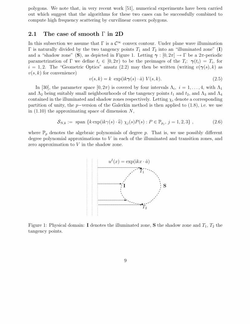
In this subsection we assume that Γ is a C∞ convex contour. Under plane wave illuminationΓ is naturally divided by the two tangency points T1 and T2 into an “illuminated zone” (I)and a “shadow zone” (S), as depicted in Figure 1. Letting γ : [0, 2π] → Γ be a 2π-periodicparametrization of Γ we define ti ∈ [0, 2π) to be the preimages of the Ti: γ(ti) = Ti, fori = 1, 2. The “Geometric Optics” ansatz (2.2) may then be written (writing v(γ(s), k) asv(s, k) for convenience)

v(s, k) = k exp(ikγ(s) · a) V (s, k). (2.5)

In [30], the parameter space [0, 2π) is covered by four intervals Λi, i = 1, . . . , 4, with Λ1

and Λ2 being suitably small neighbourhoods of the tangency points t1 and t2, and Λ3 and Λ4

contained in the illuminated and shadow zones respectively. Letting χi denote a correspondingpartition of unity, the p−version of the Galerkin method is then applied to (1.8), i.e. we usein (1.10) the approximating space of dimension N ,

SN,k := span k exp(ikγ(s) · a) χj(s)P (s) : P ∈ Ppj, j = 1, 2, 3 , (2.6)

where Pp denotes the algebraic polynomials of degree p. That is, we use possibly differentdegree polynomial approximations to V in each of the illuminated and transition zones, andzero approximation to V in the shadow zone.

uI(x) = exp(ikx · a)

I

T1

T2

S

Figure 1: Physical domain: I denotes the illuminated zone, S the shadow zone and T1, T2 thetangency points.

9

Considering the numerical analysis of this method we recall the two key questions Q1and Q2 highlighted in §1. To answer Q1 we need estimates for the dervatives of V (s, k)with respect to s which are explicit in k in the illuminated and shadow zones. Moreover weneed estimates for the exponential decay of V in the deep shadow zone Λ1. This requiresa substantial study of the theory of the “geometric optics” approximation (2.2). In [30] thefollowing result is presented.

Theorem 2.1. For all L,M ∈ N ∪ 0, the function V (s, k) admits a decomposition of theform:

V (s, k) =

[ L,M∑

ℓ,m=0

k−1/3−2ℓ/3−mbℓ,m(s)Ψ(ℓ)(k1/3Z(s))

]+RL,M(s, k) , (2.7)

for s ∈ [0, 2π], where the remainder term has its nth derivative bounded, for n ∈ N ∪ 0, by

|DnsRL,M(s, k)| ≤ CL,M,n(1 + k)µ+n/3 , (2.8)

where µ := −min

23(L+ 1), (M + 1)

and CL.M,n is independent of k. The functions bℓ,m

and Z are C∞ 2π-periodic functions. Z has simple zeros at t1 and t2, is positive-valued on[t1, t2] and negative-valued elsewhere on [0, 2π]. Moreover Ψ : C → C is an entire functionwhich may be spcified explicitly by a certain contour integral involving the Airy function (oftencalled “Fock’s integral” - see [35, §7, 12], a book originally published in the Russian literaturein the late 1940’s).

Theorem 2.1 is derived in [30] using the often cited paper [55], combined with the techniqueof matched asymptotic expansions and also referring to results from the classical literaturesuch as [18, 56, 25, 19, 69, 8].

The asymptotics of Ψ(τ) for large |τ | are of key importance for the behaviour of V . SinceZ is positive in Λ3 (inside the illuminated zone), the behaviour of V (s, k) for s ∈ Λ3 and forlarge k is determined by the asymptotics of Ψ(τ) and its derivatives as τ → ∞. Similarly,the behaviour of V (s, k) for s ∈ Λ1 (the deep shadow), depends on the asymptotics of Ψ(τ)for τ → −∞. More complicated behaviour arises in the transition zones Λ1,Λ2. The requiredproperties of Ψ are known. In particular, (see [55, Lemma 9.9]):

Ψ(τ) = a0τ + a1τ−2 + a2τ

−5 + . . .+ anτ1−3n + O(τ 1−3(n+1)) , as τ → ∞ , (2.9)

where a0 6= 0 and this expansion remains valid for all derivatives of Ψ by formally differenti-ating each term on the right hand side, including the error term. Moreover, there exists β > 0and c0 6= 0 such that, for any n ∈ N ∪ 0, as τ → −∞ ,

Dnτ Ψ(τ) = c0 D

nτ exp(−iτ 3/3 − iτα1) (1 + O(exp(−|τ |β))) , (2.10)

where α1 = exp(−2πi/3)ν1 and ν1 < 0 is the right-most root of the (all real and negative)roots of the Airy function Ai. Hence, when τ → −∞ the function Ψ, as well as its derivatives

10

decrease exponentially but in a very oscillating way. The asymptotics in (2.10) may be deducedby applying the theory of residues to the contour integral defining Ψ - see [8, p.393], [18,Lemma 8]. More details are in [30]. Combining these asymptotics with Theorem 2.1, thefollowing estimates for the derivatives of V are proved in [30].

Theorem 2.2. For all n ∈ N ∪ 0 there exist constants Cn > 0 independent of k ands ∈ [0, 2π], such that for all k sufficiently large,

|Dns V (s, k)| ≤ Cn

1, n = 0, 1,

k−1(k−1/3 + |ω(s)|)−n−2, n ≥ 2,(2.11)

where ω(s) := (s− t1)(t2 − s). These estimates are uniform in s ∈ [0, 2π].

This statement follows from [30, Theorem 5.4] but is in a somewhat simpler form thangiven there. The essential point which follows from this is that for s in the illuminated zoneand bounded away from t1, t2 (and hence |ω(s)| is bounded away from zero), all derivatives ofV are bounded as k → ∞. This shows the correctness of the Geometric Optics approximationin the interior of the illuminated zone. However, in a region of width O(k−1/3) around t1 or t2,|ω(s)| . k−1/3 and Dn

sV (s, k) may blow up with O(k(n−1)/3). (Notations like . indicate thatthere is a hidden constant independent of k). This corresponds to the estimates employed inthe analysis in [1, 2] and the motivation for the mesh grading scheme used in [12] which wehave described above.

In [30] we considered, for sufficiently large k > 0 and parameters ε, δ ∈ (0, 1/3], and c1 > 0,c2 > 0 (to be chosen), the transition zones:

Λ1 := [t1 − c2k−1/3+δ, t1 + c1k

−1/3+ε],

Λ2 := [t2 − c1k−1/3+ε, t2 + c2k

−1/3+δ] ,

and the illuminated and shadow zones, respectively:

Λ3 := [t1 + c1k−1/3+ε,, t2 − c1k

−1/3+ε] ,

Λ4 := [t2 − 2π + c2k−1/3+δ,, t1 − c2k

−1/3+δ] .

The regions Λj touch only at their endpoints.In each of the zones Λ1,Λ2 and Λ3 the error in best approximation by polynomials can

be estimated by standard methods. Using Theorem 2.2 and standard error estimates forpolynomial approximation it turns out that there are two conflicting choices for ε. The bestestimate in the illuminated zone is obtained with ε = 1/3 (i.e. the boundary of Λ1 doesnot approach t1 or t2 as k → ∞) and the best error in the transition zones is obtained withε = 0 (these zones shrink as fast as possible with k). To balance the error the best choiceturns out to be ε = 1/9. These estimates have to be combined with the following theorem onexponential decay in the deep shadow which is stated in [30].

11

Theorem 2.3. There exist positive constants c0, c′0 such that for all k sufficiently large,

‖v‖L2(Λ4) ≤ c′0 exp(−c0kδ) . (2.12)

This result can be formally inferred by using the asymptotics (2.10) in the first termof the right-hand side of (2.7), but this is not a rigorous proof since the remainder termin (2.7) enjoys only algebraically decaying estimates. A brief account of how the proof ofTheorem 2.3 follows from the results in the literature is given in [30]. In particular we refer to[63, 34, 67, 68, 52, 42, 60] for the highly non-trivial proofs. An interesting side remark is thatthe results on exponential decay (in two-dimensional problems) in [67, 68] do not require thecontour to be analytic but only sufficiently smooth. There are also extensions to arbitrarydimension, but these require analytic scattering surfaces and (as stated) are only valid in the“deep shadow” (i.e. a bounded distance away from the shadow boundary) – see, e.g. [60,Thm 3] which uses the ideas of [52].

Combining the estimate from Theorem 2.3 with the estimates for polynomial approxima-tion in the illuminated and transition zones, we obtain (in the special case pj = p for eachj = 1, 2, 3 - see [30] for more general cases), that the Galerkin method solution, defined by(1.10), satisfies the error estimate

‖v − vN‖ ≤

(B

α

)inf

φN∈SN,k

‖v(·, k) − φN‖L2(Γ) (2.13)

≤ Cn

(B

α

)k

k−4/9

(k1/9

p

)n

+ exp(−c0kδ)

. (2.14)

Here (2.13) follows from (1.7) and that, as observed after (1.10), C ≤ B/α, where B andα are the continuity and coercivity constants from (1.9). Moreover (2.14) follows from theestimates for polynomial approximation and exponential decay described above and holds forall 6 ≤ n ≤ p+1 (so in particular, for fixed k and C∞ data we have superalgebraic convergence,as is normal in the p− version of the boundary element method.)

To make the estimate (2.14) of rigorous use we have to estimate the constant B fromabove and α from below with respect to k. In [30] it is shown that for sufficiently smoothcontours Γ, and in the case η = k, we have B . k1/2. Substantial generalisations of this in[20] are discussed in §3. Estimates for α from below are much harder. In [30] it was provedby Fourier analysis (on circular or spherical boundaries) that α & 1 (i.e. k−independentcoercivity), again for η = k. However the extension of this result to general Γ is a challengingopen problem. Neverthess there is hope for success, since in [24] it was proved that ‖A−1‖ . 1for Lipschitz star-shaped Γ and any η ∈ R\0 (where A is the integral operator in (1.5)) andthis estimate is a necessary (although not sufficient) condition for k-independent coercivity ofa defined in (1.8).

On the assumption that k−independent coercivity holds for a the result (2.14) shows thatthe error in the Galerkin approximation is of the order of a low power of k times (k1/9/p)n (for6 ≤ n ≤ p + 1), plus a term which is exponentially small in k. Roughly speaking this shows

12

that by choosing p to grow slightly faster than k1/9 we preserve the accuracy of the methodas k increases. Numerical results in [30] support this result.

Before leaving this discussion we mention that using the asymptotics (2.10) when s is nearto but less than t1 (i.e. in the shadow region but near the transition point), then the firstterm in (2.7) has the asymptotics (as k → ∞) :

k−1/3b0,0 exp(ik|Z(s)|3/3) exp(iℜ(α1)k1/3|Z(s)|) exp(−ℑ(α1)k

1/3|Z(s)|) . (2.15)

Since α1 is in the first quadrant of the complex plane (see (2.10)), (2.15) contains two oscilla-tory factors, one oscillating with scale k and one with scale k1/3, damped by the exponentiallydecaying third term. These two scales were modelled in the basis functions used in the collo-cation method of Giladi and Keller, which took into account the existence of “creeping waves”behind the shadow boundary [38].

We now turn our attention to scattering by convex polygonal bodies.

2.2 The case of polygonal Γ

uI

P1 n1

Γ1

Ω1

P2

n2Γ2

Ω2

P3

n3Γ3 Ω3

P4n4

Γ4

Ω4P5

n5

Γ5

Ω5

P6

n6

Γ6

Ω6

Figure 2: Our notation for the polygon. The M corners are numbered anti-clockwise, and wedenote the first corner by both P1 and PM+1. Ωm is the exterior corner angle at Pm.

In separate work [6, 23], scattering by convex polygons, and more recently by curvilinearconvex polygons [51], has been considered. For the case of a polygon an appropriate specificform of (2.1) is shown in [23] to be

v(x, k) ≈ k exp(ikx · a)V (x, k)

+ k∑M

m=1[exp(ikx · am)V +m (x, k) + exp(−ikx · am)V −

m (x, k)],(2.16)

for x ∈ Γ, where M is the number of sides of the polygon, the unit vector am is parallel tothe mth side (directed from corner Pm to corner Pm+1 in Figure 2), and the function V ±

m is

13

assumed non-zero only on side m. (Physically the terms in the summation are included torepresent the parts of the field arising from diffraction at the corners.) In fact, it is shown in[23] that for a polygon it is adequate to take V (x, k) to be constant on each side, precisely todefine V (x, k) so that the first term in the above expression is the high frequency Kirchhoffor physical optics approximation, i.e.

∂u

∂n(x) ≈

2∂uI

∂n(x) on illuminated sides,

0, on sides in shadow.

This means to set, for x ∈ Γm,

V (x, k) :=

2inm · a, if nm · a < 0,

0, otherwise,(2.17)

where nm is the outward unit normal on side m. Then, if V ±m are approximated by piece-

wise polynomials on carefully chosen graded meshes, uniformly accurate approximations areobtained as k → ∞, provided the number of degrees of freedom grows like O(log3/2 k). Theresults [6, 23] are inspired by earlier results [22, 50] (indeed the method and analysis forthe convex polygon case are outlined in [22]). In these papers, as a prototype of develop-ing and analysing boundary element methods for high frequency scattering, high frequencyalgorithms are proposed for the problem of 2D scattering by a flat surface with piecewisecontinuous impedance boundary condition, and a complete proof of k-independent accuracyand complexity is provided, the first such result for any scattering algorithm.

We give now a little more detail of the methods and results of [23]. A key componentin the design of the ansatz (2.16) and the design of the graded meshes to approximate thefunctions V ±

m (x, k) (both of which are essential to the overall low complexity) is understandingthe high frequency behaviour of the solution. We have seen in §2.1 that obtaining rigorousresults on high frequency asymptotics is, in general, a complex business. But this case ofa convex polygon is one in which rigorous high frequency asymptotics, at least a sufficientunderstanding of these for the purpose of designing an effective numerical scheme, can beachieved by elementary arguments.

The trick (adapted from [22]) is to observe that one can write down an explicit solutionto the Dirichlet boundary value problem for the Helmholtz equation in a half-plane, sincewe (trivially) know by the method of images the Green’s function for a half-plane. Thisobservation leads to the following useful representation for the solution to the scatteringproblem. Let Dm ⊂ D denote the half-plane whose boundary contains Γm, the mth side ofthe polygon (see Figure 3), and let Gm(x, y) be the Dirichlet Green’s function for the half-plane Dm, i.e. Gm(x, y) = Φ(x, y)−Φ(x, y′m), where y′m denotes the image of y in the straightline ∂Dm. Then

u(x) = ǫm(uI(x) + uR(x)) +

∫

∂Dm

∂Gm(x, y)

∂n(y)u(y) ds(y) , for x ∈ Dm .

14

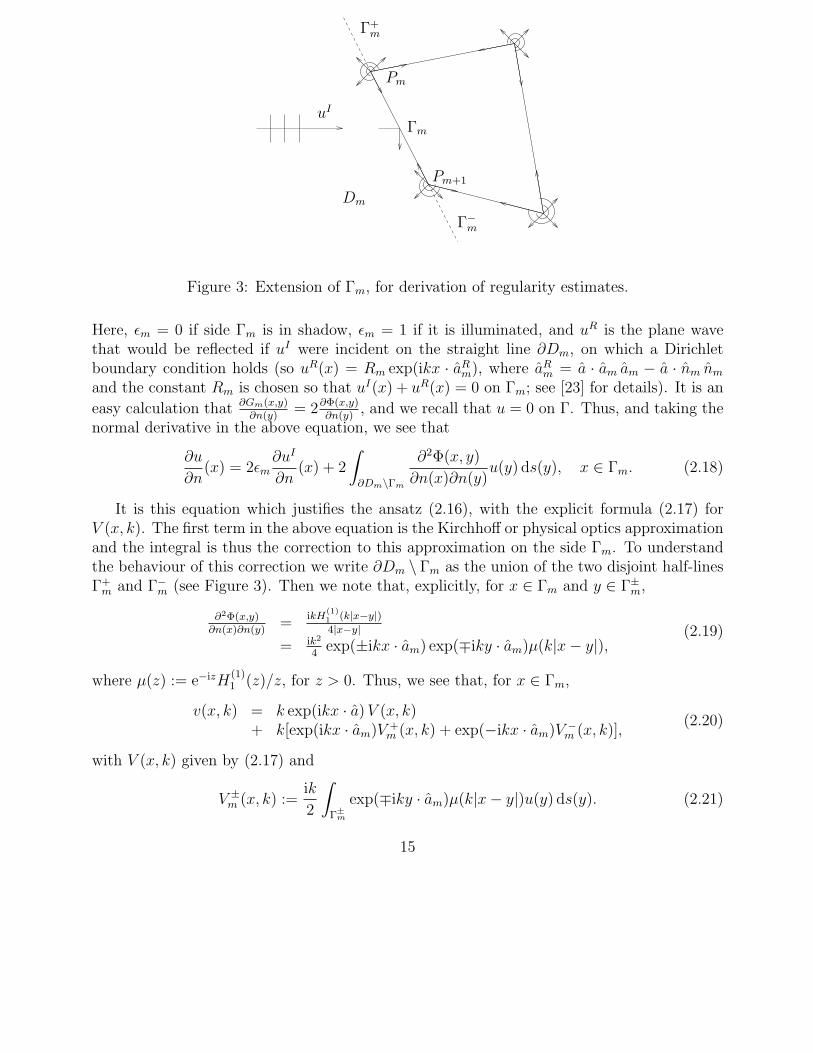
uI

Pm

Pm+1

Dm

Γm

Γ+m

Γ−m

Figure 3: Extension of Γm, for derivation of regularity estimates.

Here, ǫm = 0 if side Γm is in shadow, ǫm = 1 if it is illuminated, and uR is the plane wavethat would be reflected if uI were incident on the straight line ∂Dm, on which a Dirichletboundary condition holds (so uR(x) = Rm exp(ikx · aR

m), where aRm = a · am am − a · nm nm

and the constant Rm is chosen so that uI(x) + uR(x) = 0 on Γm; see [23] for details). It is an

easy calculation that ∂Gm(x,y)∂n(y)

= 2∂Φ(x,y)∂n(y)

, and we recall that u = 0 on Γ. Thus, and taking thenormal derivative in the above equation, we see that

∂u

∂n(x) = 2ǫm

∂uI

∂n(x) + 2

∫

∂Dm\Γm

∂2Φ(x, y)

∂n(x)∂n(y)u(y) ds(y), x ∈ Γm. (2.18)

It is this equation which justifies the ansatz (2.16), with the explicit formula (2.17) forV (x, k). The first term in the above equation is the Kirchhoff or physical optics approximationand the integral is thus the correction to this approximation on the side Γm. To understandthe behaviour of this correction we write ∂Dm \ Γm as the union of the two disjoint half-linesΓ+

m and Γ−m (see Figure 3). Then we note that, explicitly, for x ∈ Γm and y ∈ Γ±

m,

∂2Φ(x,y)∂n(x)∂n(y)

=ikH

(1)1 (k|x−y|)

4|x−y|

= ik2

4exp(±ikx · am) exp(∓iky · am)µ(k|x− y|),

(2.19)

where µ(z) := e−izH(1)1 (z)/z, for z > 0. Thus, we see that, for x ∈ Γm,

v(x, k) = k exp(ikx · a)V (x, k)+ k[exp(ikx · am)V +

m (x, k) + exp(−ikx · am)V −m (x, k)],

(2.20)

with V (x, k) given by (2.17) and

V ±m (x, k) :=

ik

2

∫

Γ±m

exp(∓iky · am)µ(k|x− y|)u(y) ds(y). (2.21)

15

The point here is that, while we cannot evaluate the integrals V ±m (x, k), because these integrals

involve the unknown u on Γ±m, we can show, in a precise quantitative way, that these functions

are not oscillatory on Γm. This is the case since µ(k|x−y|) is very smooth, except when k|x−y|is small, as the function µ(z), while singular at z = 0, is increasingly slowly varying as z → ∞,as quantified in the following lemma from [23].

Lemma 2.4. For every ǫ > 0,

|µ(m)(z)| ≤ (1 + ǫ−1/2) (m+ 1)! z−3/2−m,

for z ≥ ǫ and m = 0, 1, . . ..

Applying this lemma leads to bounds on the tangential derivatives on Γm of V ±m (x, k). In

this theorem and subsequently it is is convenient to use the abbreviation

uM := supx∈D

|u(x)|,

to let Lm denote the length of Γm, and to let ∂/∂s denote the derivative in the tangentialdirection on Γ.

Theorem 2.5. [23, Theorem 3.2] For x ∈ Γ+, let s denote the distance of x from the cornerPm. Then, for n = 0, 1, ..., it holds that

∣∣∣∣∂n

∂snV +

m (x, k)

∣∣∣∣ ≤ 2(1 + ǫ−1/2) uM n! k−1/2s−1/2−n, for ǫ ≤ ks ≤ kLm.

The same bound applies to the tangential derivatives of V −m (x, k) but with s denoting distance

along Γm from the corner Pm+1.

This bound captures the behaviour of V +m (x, k) on Γm except near the corner Pm. But

this can be understood by standard elliptic regularity estimates for behaviour of solutionsnear corners of the domain (e.g. [41]) or more explicitly by writing down a representation foru near the corner Pm based on separation of variables in polar coordinates centred on Pm

[23, theorem 2.3]. The resulting bound is the following, showing that V +m (x, k) has the classic

corner singularity behaviour near Pm where the exterior corner angle is Ωm.

Theorem 2.6. [23, Corollary 3.4] Suppose that each side of the polygon has length at leastλ/8, and, for x ∈ Γ+, let s denote distance of x from the corner Pm. Then, for n = 0, 1, ...,it holds that ∣∣∣∣

∂n

∂snV +

m (x, k)

∣∣∣∣ ≤ Cn uM k−αms−αm−n, for 0 < ks ≤ π/12,

where αm := 1 − π/Ωm ∈ (0, 1/2), and the value of the constant Cn > 0 depends only on n.The same bound applies to the tangential derivatives of V −

m (x, k) but with s denoting distancealong Γm from the corner Pm+1, and with αm replaced by αm+1.

16

The detailed information in the above bounds enables us to construct finite element spaceswhich are well-adapted to approximating the functions V ±

m . One possibility, used in [23],adapted from [26], is to use a discontinuous piecewise polynomial approximation for eachof V +

m and V −m on Γm. Thus V +

m can be approximated using piecewise polynomials of somedegree p, on a mesh which has a classical grading near the corner Pm where V +

m is singular asquantified in Theorem 2.6, and then has a geometric grading over the rest of Γm, with the twomeshes joined in a smooth manner. In detail, in the case when each side of the polygon haslength Lm ≥ λ, defining q := (2p+ 3)/(1 − 2αm), it is shown in [23] that a mesh appropriatefor approximating V +

m (x, k), given the bounds in the above theorems, consists of the points

si = λ

(i

N

)q

, i = 0, . . . , N, and sN+j := λ

(Lm

λ

)j/N+m

, j = 1, . . . , N+m. (2.22)

Here N , the number of subintervals in the interval of length λ adjacent to the corner Pm, isthe parameter controlling the mesh refinement, and N+

m is the smallest integer greater thanor equal to − log(Lm/λ)/(q log(1 − 1/N)). Based on this mesh, an appropriate piecewisepolynomial approximation space for V +

m (x, k) is

S+m = span

χj(s)P (s) : P ∈ Pp, j = 0, 1, . . . , N +N+

m

, (2.23)

where χj(s) is the characteristic function of the interval (sj−1, sj). From the mean valuetheorem applied to log(1−1/N) it follows that the number of subintervals in the geometricallygraded part of the mesh satisfies

N+m < q−1N log(Lm/λ) + 1. (2.24)

The equations defining a suitable approximation space S−m and mesh for approximating

V −m (x, k) are identical to (2.22) and (2.23), except that q is defined replacing αm by αm+1 andsi is now the distance of the mesh point from the corner Pm+1. Since the value of q is different,there is a different number N−

m of mesh points in the geometrically graded part of the mesh.Recalling (2.20), we see that an appropriate approximation space for ∂u/∂n on Γm is

k exp(ikx · a)V (x, k) + exp(ikx · am)S+m + exp(−ikx · am)S−

m, (2.25)

with V (x, k) given by (2.17). The full approximation space used in [6, 23] is the affine spaceSN,k := k exp(ikx·a)V (x, k)+SN,k, where SN,k is the linear space of functions whose restrictionto side Γm is in the set exp(ikx · am)S+

m +exp(−ikx · am)S−m, for m = 1, . . . ,M . The dimension

of SN,k, i.e. the number of degrees of freedom, is

DN = (p+ 1)∑M

m=1(2N +N+m +N−

m)< 2MN

((p+ 1)(1 +N−1) + 1

2log(L/λ)

),

(2.26)

by (2.24), where L := (L1 . . . LM)1/M .The main numerical analysis result of [23] is the following best approximation estimate:

17

Theorem 2.7. If each side of the polygon has length at least λ, then, for some positiveconstant Cp, depending only on p and on the corner angles Ω1, Ω2, . . . , ΩM , it holds that

k−1/2 infφN∈SN,k

‖v(·, k) − φN‖L2(Γ) ≤ CpuM(M [1 + log(L/λ)])p+3/2

Dp+1N

.

This theorem shows that, to maintain a given bound on the left hand side of the aboveinequality, aiming to keep (1.15) fixed as k increases, it is necessary to increase the numberof degrees of freedom DN only in proportion to (log k)3/2. If one is happy to maintain con-trol instead on k−1 infφ∈SN,k

‖v(·, k) − φ‖L2(Γ), aiming to keep (1.13) fixed, then one can evendecrease DN as k increases.

In [23] the approximation space SN,k is used as the basis of a Galerkin method for theintegral equation (1.4). Precisely, cf. (1.10), the approximation vN to v is defined by: SeekvN ∈ SN,k such that

a(vN , wN) = (f, wN)L2(Γ) , for all wN ∈ SN,k .

As discussed in §2.1, in the case that Γ is a circle it is shown in [30] that the sesquilinear forma is coercive, with a coercivity constant α independent of k. For general domains it is not yetclear whether a is coercive, and in [23] the stability analysis is approached by the classicalmethods for analysis of second kind equations discussed before equation (1.8) and in §3.1below. Using these standard methods it is shown in [23] that, for each fixed k, there existsa value for the stability constant C > 0 and an integer N0 such that the Galerkin solution iswell-defined and (1.7) holds for N ≥ N0. Combining this with Theorem 2.7 gives the estimate

k−1/2 ‖v(·, k) − vN‖L2(Γ) ≤ C CpuM(M [1 + log(L/λ)])p+3/2

Dp+1N

, (2.27)

for N ≥ N0, but, as discussed in §1 and in §3.1 below, this classical analysis does not giveany information about the dependence of C and N0 upon k. An approximation uN to u canbe computed by replacing v = ∂u/∂n by its the approximation vN in (1.3). This is shown in[23, Theorem 5.4], via the inequality (1.14), to satisfy the error bound

supx∈D |u(x) − uN(x)|

supx∈D |u(x)|≤ C C ′

p

(M [1 + log(L/λ]))p+2

Dp+1N

, (2.28)

for N ≥ N0, where C ′p is a positive constant depending only on p and the corner angles Ω1,

Ω2, . . . , ΩM . Numerical results supporting these error estimates are shown in [23].A collocation method based on the identical approximation space SN,k and the identical

integral equation formulation is implemented in [6]. No stability analysis (even one based onclassical second-kind theory) is made in [6], but the numerical results support the conclusionthat there is little difference in accuracy between the Galerkin and the (rather easier toimplement) collocation method.

18

3 Stability and Conditioning

3.1 General considerations

In §1 we have split the numerical analysis of high frequency boundary element methods intoresearch on three related questions. We turn in this section to research related to the sec-ond of these questions, namely the problem of estimating the value of the stability constantC in (1.7). We note that, while the emphasis of this review is on boundary integral equa-tion methods specifically adapted to high frequency scattering, the results of this section areequally applicable to stability analysis and conditioning for conventional piecewise polynomialboundary element methods at high frequency.

We have noted already that, in the case that the sesquilinear form a is coercive, an upperbound on the stability constant C in the case when vN is defined by the Galerkin method (i.e.by (1.10)) is

C ≤B

α(3.1)

where B and α are the continuity and coercivity constants in (1.9). These constants are closelyrelated to the norms of A′ and its inverse as operators on L2(Γ). Indeed, by Cauchy-Schwarz,for v, w ∈ L2(Γ) (and with ‖ · ‖ denoting throughout the norm of a bounded linear operatoron L2(Γ)),

|a(v, w)| = |(A′v, w)L2(Γ)| ≤ ‖A′v‖L2(Γ) ‖w‖L2(Γ)

≤ ‖A′‖ ‖v‖L2(Γ) ‖w‖L2(Γ).

Thus ‖A′‖ is a possible value for the constant B in (1.9). In fact (as follows from settingw = A′v in the above inequality), ‖A′‖ is the smallest possible value for the constant B forwhich (1.9) holds. Similarly, from the second of the inequalities (1.9),

‖A′v‖L2(Γ) ‖v‖L2(Γ) ≥ |(A′v, v)L2(Γ)| = |a(v, v)| ≥ α‖v‖2L2(Γ),

so that‖A′−1

‖ ≤ α−1.

Thus, the ratio B/α is bounded below by the condition number of the operator A′:

B

α≥ cond A′ := ‖A′‖ ‖A′−1

‖. (3.2)

This gives one motivation for studying the condition number of A′ and its dependenceon k, which will be a main topic of this section. Another motivation is the following. Theinequality (3.1) is only useful if a is coercive, which we will see below is known to be the caseif Γ is a circle or sphere, but not, so far, more generally. Whether or not a is coercive, it is

19

known that the Galerkin method (1.10) is well-defined if and only if a satisfies the discreteinf-sup condition: that, for some γN > 0 (the discrete inf-sup constant),

sup06=w∈SN,k

|a(v, w)|

‖w‖L2(Γ)

≥ γN‖v‖L2(Γ), for v ∈ SN,k. (3.3)

If (3.3) holds (which it does, for example, if a is coercive, with γN = α), then a standardupper bound for the stability constant C is

C ≤ 1 +B

γN

. (3.4)

We do not know of any explicit bounds on the discrete inf-sup constant for high frequencyboundary element methods, but we note that ‖A′−1‖ = γ−1, where γ is the correspondingcontinuous inf-sup constant, i.e.

γ := inf06=v∈SN,k

sup06=w∈SN,k

|a(v, w)|

‖v‖L2(Γ) ‖w‖L2(Γ)

. (3.5)

Thus, if B is the smallest value for which the left-hand inequality in (1.9) holds, then

cond A′ =B

γ.

One can hope that studying cond A′ sheds some light on the behaviour, e.g. as a function ofk and the coupling parameter η, of B/γN and hence of the upper bound (3.4).

As mentioned in §1, stability can also be studied by classical second-kind integral equationmethods [7]: these have the attraction that they also apply to classes of collocation methods,indeed to projection methods in general. Focusing on the Galerkin case, introducing theoperator PN of orthogonal projection from L2(Γ) to SN,k, and writing A′ as A′ = I + K, sothat K = D′ − iηS, it can be shown (e.g. [7]) that the formulation (1.10) is equivalent to theoperator equation

(I − PNK)vN = PNf,

and that the Galerkin method is well-defined if and only if I −PNK is invertible. Moreoever,if the Galerkin method is well-defined, then

v − vN = (I − PNK)−1(v − PNv). (3.6)

Thus a possible value for the stability constant C in (1.7) is

C = ‖(I − PNK)−1‖.

In the case that Γ is C1, so that K is compact [33, 27], the classical results tell us that, as longas the spaces SN have the standard approximation property that infφN∈SN

‖φ− φN‖L2(Γ) → 0as N → ∞, for every φ ∈ L2(Γ), then ‖PNK −K‖ → 0 as N → ∞. Thus

C = ‖(I − PNK)−1‖ → ‖(I −K)−1‖ = ‖A′−1‖

20

as N → ∞ (with k fixed). Alternatively, one can write (3.6) as

v − vN = (I + LN)(v − PNv), where LN := (I − PNK)−1PNK(I − PN), (3.7)

from which equation it is clear that (1.7) holds with

C = 1 + ‖LN‖ .

When K is compact it holds that ‖LN‖ → 0 as N → ∞ (since ‖K −KPn‖ → 0). Thus wesee that, at least in the case that Γ is C1, the bound (1.7) holds for every C > 1 provided Nis sufficiently large (N ≥ N0). However, as we have emphasised already in §1, it is not clear,for a fixed value of C > 1, how large N0 needs to be for (1.7) to hold, and how this valueN0 depends on k. More fundamentally, for Galerkin methods based on hybrid approximationspaces, such as we have discussed in §2, it is the aim to keep N fixed or almost fixed as k → ∞,so that it is not clear that we will ever be in the regime where KPN is a good approximation toK in operator norm so that we can prove that ‖LN‖ ≈ 0. On the other hand, it is reasonableto hope that ‖(I − PNK)−1‖ will be well-approximated by ‖(I − K)−1‖ = ‖A′−1‖ before‖PNK −K‖ is small, in which case (1.7) will hold with

C ≈ ‖A′−1‖.

We have summarised what the known variational-based and classical second-kind integralequation techniques can tell us about the stability constant C. For a recent analysis which is,roughly speaking, intermediate between the two techniques, and its application to the erroranalysis of conventional boundary integral equation methods at high frequency, see [9].

In the next subsection we discuss what is known about the coercivity constant α, the con-tinuity constant B (the smallest choice for which is ‖A′‖), ‖A′−1‖, and cond A′ = ‖A′‖ ‖A′−1‖,and their dependence on the wavenumber k and the coupling parameter η in (1.5).

3.2 Coercivity and condition numbers

Studies of the conditioning and spectral properties of integral operators (and their discreti-sations) in acoustic and electromagnetic scattering date back to Kress and Spassov [49] (andsee [48, 3, 4, 37, 66, 65, 64, 17, 30, 24, 20]). Most studies have focussed on the special casewhen Γ is a circle or sphere in which case a very complete theory is possible due to the factthat all the integral operators S, D, D′ and H, defined in §1, operate diagonally in the basisof trigonometric polynomials (d = 2) or spherical harmonics (d = 3). The analysis is furthersimplified by the fact that D = D′ and so A = A′ when Γ is a circle/sphere.

Suppose Γ is the unit circle, with parametrisation γ(s) = (cos s, sin s). With this parametri-sation L2(Γ) is isometrically isomorphic to L2[0, 2π]. We can write any w ∈ L2[0, 2π] = L2(Γ)as

w(s) =1

2π

∑

m∈Z

wm exp(ims), where wm :=

∫ 2π

0

ϕ(s) exp(−ims) ds,

21

in which case the L2-inner product and norm are given by (v, w)L2(Γ) = 12π

∑m∈Z

vmwm and‖w‖2

L2(Γ) = 12π

∑m∈Z

|wm|2. Then (see [48, equation (4.4)] or [30, Lemma 4.1]), we have the

Fourier representation:

A′w(s) = 12π

∑m∈Z

λmwm exp(ims)

with λm = πH(1)|m|(k)

[ikJ ′

|m|(k) + ηJ|m|(k)].

(3.8)

Note that λm is the eigenvalue of A′ = A corresponding to the eigenfunction exp(±ims). Asargued in [48], since the eigenfunctions exp(ims), m ∈ Z, are a complete orthonormal systemin L2[0, 2π] = L2(Γ), it holds that

‖A′‖ = supm∈N∪0

|λm|, ‖A′−1‖ =

(inf

m∈N∪0|λm|

)−1

, (3.9)

so that

cond A′ =supm∈N∪0 |λm|

infm∈N∪0 |λm|. (3.10)

Further, for w ∈ L2(Γ) we have that

|a(w,w)| = |(A′w,w)L2(Γ)| ≥ ℜ(A′w,w)L2(Γ)

=1

2π

∑

m∈Z

ℜ(λm)|wm|2 ≥ α‖w‖2

L2(Γ),

whereα = inf

m∈N∪0ℜ(λm). (3.11)

For the case d = 3, when Γ is a sphere of unit radius, a similar analysis applies, basedon the fact that the integral operators on the sphere are diagonal operators in the space ofspherical harmonics. The corresponding expression for the symbol λm is

λm = ikh(1)m (k) (kj′m(k) + iηjm(k)) , (3.12)

where jm and h(1)m are the spherical Bessel and Hankel functions respectively. This formula

can be found, for example, in [48, 37] – see also [17]. The formulae (3.9), (3.10), and (3.11)hold also in the 3D case [48, 30], with λm given by (3.12).

We see that, for the case of a circle/sphere, studying the coercivity and conditioning ofA′ reduces to the study of the behaviour of explicitly known eigenvalues λm, as a function ofm, the wavenumber k, and the coupling parameter η. The early papers [49, 48] carried outa precise theoretical and numerical study of this issue for the case of small k, with emphasison choosing η so as to minimise the condition number. The thesis of Giebermann [37] madea similar careful study of the large k case, which is our main focus here, with a mixture ofrigorous analysis, indicative asymptotics, and numerical calculation. The substantial gaps in

22

the analysis in [37] (in particular, the estimates of the coercivity constant α in [37] were sug-gestive rather than rigorous: the issue is to obtain sufficiently sharp bounds on the relevantcombinations of Bessel functions that are uniform in argument and order) were filled recentlyin [30], for the explicit choice η = k (previously proposed as optimal for conditioning for theunit circle when k ≥ 1 in e.g. [49, 3, 4]). Further, one of the bounds in [30] was refinedrecently in [9] (an improved upper-bound on the norm of D, the double-layer operator partof A′). Additionally, there are techniques and results that we shall mention below, describedin [24, 20], that apply to general boundaries, and so to the circle/sphere in particular. Theupshot (see [20] for more historical detail) is that the following results are now known for thecircle/sphere. In all these bounds c ≥ 1 denotes some absolute constant, not necessarily thesame at each occurrence.

Coercivity for the circle/sphere ([30, 20]). With the choice of coupling parameter η = k,A′ = A is coercive for all sufficiently large k, with α bounded above and below by constantsindependent of k. Indeed, for the circle,

α = 1 for all sufficiently large k.

Conditioning for the circle/sphere ([30, 20]).

1 ≤ ‖A′−1‖ = ‖A−1‖ ≤ c

(1 +

1 + k

η

); (3.13)

indeed, for a circle and η = k it holds that ‖A′−1‖ = ‖A−1‖ = 1 for all sufficiently large k.For a sphere,

1 ≤ ‖A′‖ = ‖A‖ ≤ c(1 + η(1 + k)−2/3

); (3.14)

the same bound holds for a circle in the case η = k. Thus, for a sphere,

cond A′ = cond A ≤ c(1 + k1/3

), (3.15)

if η = 1 + kp, for some p ∈ [2/3, 1]. The same bound holds for a circle, for k ≥ 1, with thechoice η = 1 + k.

We note that the above bounds (3.13)–(3.15) suggest that taking η = 1 + kp, for somep ∈ [2/3, 1] will be approximately optimal in terms of minimising the condition numbers of A′

and A. In fact, for a sphere of radius R0, based on low frequency calculations and analysis,the specific choice

η = max

(1

2R0

, k

)(3.16)

was made in [48], and there is further evidence supporting this choice for higher frequencies in[3, 4]. Recently, Banjai and Sauter [9] have pointed out that, as is clear from (3.15), choosingη = k2/3 gives the same growth rate as k → ∞ as the choice η = k, and calculations for the

23

case of a circle confirm almost identical values of condition number for η = k/2 and η = k2/3

at high wavenumbers.In recent work by the authors and their collaborators [30, 24, 20, 21] rigorous upper and

lower bounds on ‖A‖ = ‖A′‖ and ‖A−1‖ = ‖A′−1‖ have been obtained for rather general classesof scatterers, which results show that: (i) the detail of the geometry of Γ plays a strong role indetermining the dependence of these norms on k; (ii) the growth of the condition number withk can be much faster than the mild growth (3.15) for a circle/sphere. We briefly summarisethe techniques that have been used and the results that have been obtained.

A first, simple, observation [20, Lemma 4.1] is that both ‖A′‖ and ‖A′−1‖ are boundedbelow by the value 1, as a consequence of being perturbations of the identity, if some partof Γ is at least C1 smooth. To obtain upper bounds on ‖A′‖ rather crude methods are usedin [20] which ignore the oscillation in the kernels of the integral operators D′ and S (whosenorms are bounded separately, and then ‖A′‖ is bounded using the triangle inequality). Forexample, we bound ‖S‖ using the estimate

‖S‖ ≤ 2 supx∈Γ

∫

Γ

|Φ(x, y)| ds(y) ≤ k(d−3)/2(2π)(1−d)/2

∫

Γ

ds(y)

|x− y|(d−1)/2, (3.17)

the last inequality in fact an equality in the 3D case (d = 3). Our resulting bound on thenorm of A′ is the following:

Theorem 3.1. [20, Theorem 3.6] For every Lipschitz Γ, there exist positive constants c1 andc2, dependent only on Γ, such that

‖A‖ = ‖A′‖ ≤ 1 + c1k(d−1)/2 + c2ηk

(d−3)/2,

for all k > 0.

In 2D (d = 2), for the case Γ simply-connected and smooth, this bound was shown previ-ously, for all sufficiently large k, in [30].

We note that these bounds predict, for the usual choice η = k, a faster growth than(3.14) for a circle/sphere as k increases, namely proportional to k1/2 in 2D, k in 3D. Perhapssurprisingly, although the techniques used to obtain the above bounds ignore the increasingoscillation in the kernels of the integral operators as k increases, it is shown in [20] that in 2D(nothing is known yet about the 3D case) the above bounds are sharp, in the sense that thereexist Lipschitz boundaries Γ for which ‖S‖ grows proportional to k−1/2 and ‖D′‖ arbitrarilyclose to k1/2. In particular:

Lemma 3.2. [20, Theorem 4.2] In the 2D case, if Γ contains a straight line section of lengtha, then

‖S‖ ≥

√a

πk+O(k−1)

as k → ∞ and

‖A‖ = ‖A′‖ ≥ η

√a

πk− 1 +O(ηk−1)

24

as k → ∞, uniformly in η > 0.

The quantitative information in the above lemma is pretty sharp. Indeed if Γ is a straightline of length a then the formula (3.17) tells us that

‖S‖ ≤ 2

√a

πk.

The technique used to obtain Lemma 3.2 is to construct a φk ∈ L2(Γ), dependent onthe wavenumber k, so as to approximately maximise ‖Sφk‖L2(Γ)/‖φk‖L2(Γ). For the proof ofLemma 3.2 the choice φk(x) = exp(ikx · c) on the straight line part of Γ, and zero elsewhereon Γ, where the unit vector c is parallel to the straight line section of Γ, does the trick.

The same technique can be used to construct lower bounds that explore the subtle inter-action between the geometry and the size of ‖S‖ and ‖D‖ = ‖D′‖. For example, one resultfrom [20] is (cf. the bound (3.14) for the case of a circle/sphere):

Lemma 3.3. [20, Corollary 4.5] Suppose (in the 2D case) that Γ is locally C2 in a neighbour-hood of some point x∗ on the boundary and let R be the radius of curvature at x∗. If R <∞,then, as k → ∞,

‖S‖ ≥1

2

(R

π

)1/3

(2k)−2/3(1 + o(1)). (3.18)

If also ηk−2/3 → ∞ as k → ∞, then also

‖A′‖ = ‖A‖ ≥η

2

(R

π

)1/3

(2k)−2/3(1 + o(1)),

as k → ∞.

Other results in [20] explore what happens if the radius of curvature vanishes (and otherhigher order smoothness conditions) and under what conditions ‖D′‖ = ‖D‖ can be large.The lower bounds in the above lemmas meet the upper bounds in Theorem 3.1 in some cases.For example, if Γ is a polygon (as in §2.2) and the usual choice η = k is made then, for someconstants c1 and c2,

c1k1/2 ≤ ‖A′‖ = ‖A‖ ≤ c2k

1/2,

for all sufficiently large k. In other cases, for example for an ellipse or some other smooth,strictly convex obstacle, there is a gap between our upper and lower bounds: e.g. for η = kour upper bound (Theorem 3.1) gives a growth rate of k1/2 while our lower bound (Lemma3.3) has a growth rate of k1/3. We suspect, from the case of the circle (3.14), and from theevidence of numerical simulations in [21], that it is our lower bounds that are sharp.

One technique that has not been employed yet to obtain upper bounds, which is standardin the harmonic analysis literature [61], and which could be the tool to close the gap, is theobservation that, e.g.

‖D′‖ = ‖D‖ = ‖DD∗‖1/2.

25

Here D∗ is the Hilbert space adjoint of D (whose kernel is the complex conjugate of the kernelof D′). The point is that DD∗ is itself an integral operator whose norm can be estimatedby the (relatively crude) methods we use to prove Theorem 3.1, and that the kernel of theintegral operator DD∗ is given as an oscillatory integral involving the wavenumber k, whosevalues may be estimated by standard oscillatory integral techniques [61].

To provide upper bounds on ‖A′−1‖ = ‖A−1‖ a completely different technique has beenused, namely a priori bounds derived from Rellich-type identities and subtle properties ofradiating solutions of the Helmholtz equation [24]. These upper bounds apply for a generalclass of geometries, namely whenever the scatterer Ω is simply-connected, piecewise smooth,starlike, and Lipschitz. For the rest of this section we assume, without loss of generality, thatthe origin lies in Ω (0 ∈ Ω). Then the class of domains studied in [24] are those satisfying thefollowing assumption (Assumption 3 in [24]):

Assumption 3.4. Γ is Lipschitz and is C2 in a neighbourhood of almost every x ∈ Γ. Further

δ− := ess infx∈Γ

x · n(x) > 0.

Note that Assumption 3.4 holds, for example, if Ω is a convex polyhedron (and 0 ∈ Ω),with δ− the distance from the origin to the nearest side of Γ.

Define

R0 := supx∈Γ

|x|, δ+ := ess supx∈Γ

x · n(x), δ∗ := ess supx∈Γ

|x− (x · n(x))n(x)|.

Then a main result in [24] is the following:

Theorem 3.5. Suppose that Assumption 3.4 holds and η > 0. Then

‖A′−1‖ = ‖A−1‖ ≤ B (3.19)

where B is given by the formula:

1

2+

[(δ+δ−

+4δ∗2

δ2−

)[δ+δ−

(k2

η2+ 1

)+d− 2

δ−η+δ∗2

δ2−

]+

(1 + 2kR0)2

2δ2−η

2

]1/2

.

To understand this expression for B, suppose first that Γ is a circle or sphere, i.e. Γ = x :|x| = R0. Then δ− = δ+ = R0 and δ∗ = 0 so

B = B0 :=1

2+

[1 +

k2

η2+d− 2

R0η+

(1 + 2kR0)2

2R20η

2

]1/2

. (3.20)

In the general case, since δ− ≤ δ+ ≤ R0 and 0 ≤ δ∗ ≤ R0, it holds that B ≥ B0. Note that theexpression B blows up if k/η → ∞ or if δ+/δ− → ∞, or if δ−η → 0, uniformly with respectto the values of other variables.

26

An important implication of Theorem 3.5 is that, whenever Γ is starlike in the sense ofAssumption 3.4, if η is chosen so that

max(l1R−10 , l2k) ≤ η ≤ max(u1R

−10 , u2k), (3.21)

for some positive constants l1, l2, u1, and u2, then, for some constant c > 0, ‖A′−1‖ = ‖A−1‖ ≤c, for all k > 0. For example, choosing

η = R−10 + k, (3.22)

which satisfies (3.21) with l1 = l2 = 1 and u1 = u2 = 2, defining θ := R0/δ−, and noting thatδ+/δ− ≤ θ, δ∗/δ− ≤ θ, we see that Theorem 3.5 implies that

‖A′−1‖ = ‖A−1‖ ≤ B ≤

1

2+ θ[2 + (1 + 4θ)(d+ θ)]. (3.23)

Based on computational experience, Bruno and Kunyansky [15, 16] recommend the choiceη = max(6T−1, k/π), where T is the diameter of the obstacle, which satisfies (3.21), thisformula chosen on the basis of minimising the number of GMRES iterations in an iterativesolver. Another choice of η satisfying (3.21) is (3.16), recommended as optimal for a spherefor low frequency in [48].

Putting together the bounds of Theorems 3.1 and 3.5, we see that, in the case when Γ ispiecewise C2, Lipschitz and starlike, satisfying Assumption 3.4, it holds, for some constantc ≥ 1 depending on Γ, that

1 ≤ cond A′ = cond A ≤ c(1 + k(d−1)/2 + ηk(d−3)/2

) (1 +

1 + k

η

). (3.24)

Thus, for some constant c′ ≥ 1,

1 ≤ cond A′ = cond A ≤ c′(1 + k(d−1)/2

), (3.25)

if η is chosen to satisfy (3.21), e.g. given specifically by (3.16) or (3.22).If Γ is not starlike then ‖A′−1‖ = ‖A−1‖ can grow as k increases. In particular, a 2D

example is presented in [20, 21] in which Γ is a trapping-type obstacle, with two straightparallel sides separated by the medium of propagation. It is shown in [20], by combiningarguments from [24] with methods of estimating multi-dimensional oscillatory integrals from[47], that, for some constant c > 0,

‖A′−1‖ = ‖A−1‖ ≥ ck9/10(1 + η/k)−1

and thatcond A′ = cond A ≥ c(1 + k14/10)

for the usual choice of η satisfying (3.21).

27

4 Implementation

This paper has concentrated on the theory of integral equation formulations for the Helmholtzequation and their numerical solution by Galerkin and collocation methods in the high-frequency case. A hugely important question, which we only have space to deal with briefly,is whether these methods can be realised with computation times which are reasonable ask → ∞, in particular, do the computation times reflect the theoretical estimates which wehave given above? We describe briefly in this section, work on two different issues which arerelated to this question.

Computation of Oscillatory Stiffness Matrix Entries.The Galerkin and collocation methods described above require work on the assembly of stiff-ness matrices, the entries of which are given as oscillatory integrals. The Nystrom approachof Bruno et. al. [12, 13] involves a direct approach to the integration problem, without theintermediate step of considering it as part of an expansion method for the integral equation.In any case oscillatory integrals defined on (subsets of) obstacle boundaries with, in addition,weakly singular integrands and complicated phase functions must be computed.

In particular, the hybrid Galerkin discretisation (with (2.1)) of the representative integraloperator v(x) 7→

∫ΓΦ(x, y)v(y)ds(y) taken from (1.4), leads to double integrals of the form

∫

Sn′

∫

Sn

Φ(x, y) exp(ik[γm(y) − γm′(x)])

Pn(y)Pn′(x)ds(y)ds(x) , (4.1)

where the Pn are (piecewise) polynomial basis functions with supports Sn. Because the phaseof the fundamental solution Φ is known, the kernel (in the braces) in (4.1) may also be writtenas exp(ik[|x−y|+γm(y)−γm′(x)])K(x, y), withK (weakly) singular but non-oscillatory, reveal-ing an oscillatory double integral with a complicated geometry-dependent phase. Collocationmethods lead to the simpler (but still oscillatory) single integrals:

∫

Sn

Φ(x, y) exp(ik[γm(y) − γm′(x)])

Pn(y)ds(y) , (4.2)

to be evaluated at collocation points x.There has been considerable recent activity on problems of oscillatory integration in general

(e.g. [46], [47]), which has provided new insight and analysis for classical methods such asFilon’s rule and Levin’s method, and, by particularly exploiting asymptotic theory, has alsogenerated new classes of methods. We refer to the separate review [45] in this volume formore detail.

Building on the progress on oscillatory integration in general, Huybrechts and Vandewalle[44] described a general method for computing integrals of the form (4.2) using a numericalvariant of the method of steepest descent, in which the integral over Sn (parametrised by a realinterval) is computed via an integral over a path in the complex plane over which the integrandis not oscillatory. A very nice observation which then follows is that if the collocation point x

28

is not in Sn, if the phase has no stationary points, and if Pn has sufficiently many vanishingderivatives then (4.2) vanishes rapidly as k increases. Hence if local basis functions are usedin the collocation method, then the collocation matrix can be replaced by a sparse matrix forlarge k. The only non-zero entries of the sparse matrix correspond to points x and supports Sn

where either x ∈ Sn (a “singular point”), or the phase has a stationary point. Although thereis no stability analysis of the method in [44], the numerical results suggest this idea producesa powerful novel algorithm. This idea was further developed in [43, 62] in the context ofthe partition of unity boundary integral method with plane wave basis functions, appliedto general Helmholtz problems (as distinct from the plane wave scattering considered here).In this case the oscillatory integrals can contain very complicated distributions of stationarypoints.

An application of the method of stationary phase to the computation of collocation ma-trices arising in boundary integral methods with global basis functions on domains which arediffeomorphic to the sphere is presented in [36]. There the chief difficulty is the problem oflocating the stationary points for general geometries.

When choosing quadrature rules for implementing boundary integral methods in the highfrequency case, one should bear in mind error estimates for the solution of the integral equationsuch as (2.14) and Theorem 2.7. It is clear that one requires sharp quadrature error estimatesas N → ∞ with explicit dependence on k in the asymptotic constant. When we applyquadrature to approximate the stiffness matrix for these methods, we only need to ensurethat the resulting perturbations satisfy the same kind of error estimates and can then applyclassical “Strang Lemma” arguments to obtain error estimates for the whole practical method.Progress on this issue for the 2D Galerkin case on a polygon in the context of hp-Galerkinmethods has been made by Melenk and Langdon [54]. This approach employs a change ofvariable of the form τ = |x− y|+ γm(y)− γm′(x) for either fixed x or y. This ensures that theoscillation in (4.1) is in one variable only, and then applies Filon quadrature. However muchwork remains to prove rigorous error estimates and extend the results to 3D.

In an intriguing different approach [28] computes integrals such as (4.1) on a subgridwhich resolves the oscillations and does this efficiently using a multipole expansion of thekernel factor Φ(x, y) for (x, y) in each block of a tree-based decomposition of Γ× Γ. This is apractical alternative to difficult stationary-phase based methods.Fast methods for dense systems. Matrix compression and fast solvers for non-local op-erator equations are a major development in numerical analysis in the last 25 years. Typi-cal solvers usually consist of a (preconditioned) Krylov iterative method coupled with a fastmatrix-vector multiplication based on kernel approximation (e.g. multipole or panel clustering,or more recently H-matrices). The fast multiplication algorithms work by approximating the(weakly singular) kernel K(x, y) by combinations of separable functions of the form ai(x)bj(y)when x, y are sufficiently separated. Blocks of the dense stiffness matrix are thus replacedby low rank matrices, with the choice of blocking and approximation controlled by a tree-based hierarchical algorithm. This allows matrix-vector multiplications with the N×N denseboundary element stiffness matrix in close to O(N) time. This method has been extended to

29

high frequency Helmholtz problems approximated by conventional boundary elements (e.g.[26, 29]), but the extension to hybrid approximations is an open and fascinating problem.This is important, especially in 3D, since then, even using the hybrid approximation spacesproposed above, N may still be large. The results of [28] show that replacing the Helmholtzkernel with a separable expansion in the far field can still yield low rank approximations evenin the hybrid case, but much work remains to be done to yield a solver for which the cost isclose to O(N) with a k-independent constant.

Acknowledgement: We would like to thank Valery Smyshlyaev for guiding us throughthe substantial literature in this field from the former Soviet Union.

References

[1] Abboud, T., Nedelec, J.-C., Zhou, B. (1994). Methode des equations integrales pour leshautes frequencies. C.R. Acad. Sci. Paris. 318 Serie I, 165–170.

[2] Abboud, T., Nedelec, J.-C., Zhou, B. (1995). Improvement of the integral equationmethod for high-frequency problems, in Proceedings of 3rd International Conference onMathematical Aspects of Wave Propagation Problems (SIAM, Phildelphia).

[3] Amini, S. (1990). On the choice of the coupling parameter in boundary integral formula-tions of the exterior acoustics problem. Appl. Anal. 35, 75–92.

[4] Amini, S. (1993). Boundary integral solution of the exterior acoustic problem, Comput.Mech. 13, 2–11.

[5] Anand, A., Boubendir, Y., Ecevit, F. and Reitich, F. (2006). Analysis of multiplescattering iterations for high-frequency scattering problems II: The three-dimensionalscalar case, report 147, Max-Planck-Institut fur Mathematik in den Naturwissenschaften,Leipzig.

[6] Arden, S., Chandler-Wilde, S. N. and Langdon, S. (2007). A collocation method for highfrequency scattering by convex polygons. J. Comp. Appl. Math. , 204 334–343.

[7] Atkinson, K. E. (1997). The Numerical Solution of Integral Equations of the Second Kind,(Cambridge University Press, Cambridge).

[8] Babich, V.M., Buldyrev, V.S. (1991). Short-wavelength Diffraction Theory (Springer-Verlag, Berlin).

[9] Banjai, L. and Sauter, S. (2007). A refined Galerkin error and stability analysis for highlyindefinite variational problems, SIAM J. Numer. Anal. 45 37–53.

30

[10] Bonner, B.D., Graham, I.G. and Smyshlyaev, V.P. (2005). The computation of conicaldiffraction coefficients in high frequency acoustic wave scattering, SIAM J. Numer. Anal.43, 1202–1230.

[11] Brakhage, H. and Werner, P. (1965). Uber das Dirichletsche Außenraumproblem fur dieHelmholtzsche Schwingungsgleichung, Arch. Math. 16, 325–329.

[12] Bruno, O.P., Geuzaine, C. A., Monro, J.A. Reitich, F. (2004). Prescribed error toleranceswithin fixed computational times for scattering problems of arbitrarily high frequency:the convex case. Phil. Trans. R. Soc. Lond. A. 362, 629–645.

[13] Bruno, O.P. and Geuzaine, C. A. (2007). An O(1) integration scheme for three-dimensional surface scattering problems, J. Comp. Appl. Math. , 204 , 463–476.

[14] Bruno, O.P., Geuzaine, C.A., Reitich, F. (2005). On the O(1) solution of multiple-scattering problems, IEEE Trans. Magn. 41, 1488-1491.

[15] Bruno, O.P. and Kunyansky, L. (2001). Surface scattering in three dimensions: an accel-erated high-order solver, Proc. R. Soc. Lond. A 457, 2921-2934.

[16] Bruno, O.P. (2007). Private communication.

[17] Buffa, A. and Sauter, S. (2006). On the acoustic single layer potential: Stabilisation andFourier analysis, SIAM J. Sci. Comput. 28, 1974–1999.

[18] Buslaev, V. S. (1964). Short-wave asymptotic behaviour in the problem of diffraction bysmooth convex contours (in Russian), Trudy Mat. Inst. Steklov. 73, 14–117. AbbreviatedEnglish summary: On the shortwave asymptotic limit in the problem of diffraction byconvex bodies, Soviet Physics Doklady 7, 685–687. (1963)

[19] Buslaev, V.S. (1975). The asymptotic behavior of the spectral characteristics of exteriorproblems for the Schrodinger operator (in Russian). Izv. Akad. Nauk SSSR Ser. Mat. 39,149–235; English translation (1975). Math. USSR–Izv. 9, 139-223.

[20] Chandler-Wilde, S. N., Graham, I. G., Langdon, S., and Lindner, M. (2007). Conditionnumber estimates for combined potential boundary integral operators in acoustic scat-tering, Isaac Newton Institute for Mathematical Sciences Preprint NI07067-HOP, IsaacNewton Institute.

[21] Chandler-Wilde, S. N., Graham, I. G., Langdon, S., and Lindner, M. (2007). Condi-tion number estimates for combined potential integral operators in acoustics and theirboundary element discretisation, in preparation.

[22] Chandler-Wilde, S. N., Langdon, S. and Ritter, L. (2004). A high-wave numberboundary-element method for an acoustic scattering problem, Phil. Trans. R. Soc. Lond.A. 362, 647–671.

31

[23] Chandler-Wilde, S. N. and Langdon, S. (2007). A Galerkin boundary element methodfor high frequency scattering by convex polygons, SIAM J. Numer. Anal. 45, 610–640.

[24] Chandler-Wilde, S. N. and Monk, P. (2008). Wave-number-explicit bounds in time-harmonic scattering, SIAM J. Math. Anal. 39, 1428-1455.

[25] Chazarain, J. (1973). Construction de la parametrix du probleme mixte hyperboliquepour l’equation des ondes, C. R. Acad. Sc. Paris 276, 1213–1215.

[26] Chew, W.C., Song, J.M. , Cui, T.J., Velamparambil, S., Hastriter, and Hu, B. (2004).Review of large scale computing in electromagnetics with fast integral equation solvers,Computer Modeling in Engineering and Sciences, 5, 361-372.

[27] Colton. D. and Kress, R. (1983). Integral Equation Methods in Scattering Theory (Wiley,New York).

[28] Darrigrand, E. (2002). Coupling of fast multipole method and microlocal discretizationfor the 3-D Helmholtz equation, J. Comput. Phys. 181, 126–154.

[29] Darve, E. and Have, P. (2004). A fast multipole method for Maxwell equations stable atall frequencies, Phil. Trans. R. Soc. Lond. A, 362, 603–628.

[30] Dominguez, V., Graham, I.G. and Smyshlyaev, V.P. (2007). A hybrid numerical-asymptotic boundary integral method for high-frequency acoustic scattering, Numer.Math. 106, 471–510.

[31] Ecevit, F. (2005). Integral equation formulations of electromagnetic and acoustic scatter-ing problems: convergence of multiple scattering iterations and high-frequency asymp-totic expansions. PhD Thesis, University of Minnesota.

[32] Ecevit, F., Reitich, F. (2006). Analysis of multiple scattering iterations for high-frequencyscattering problems. I: The two dimensional case, report 137, Max-Planck-Institut furMathematik in den Naturwissenschaften, Leipzig.

[33] Fabes, E. B., Jodeit, M. and Riviere, N.M. (1978). Potential techniques for boundaryvalue problems on C1 domains, Acta Math., 141, 165–186.

[34] Filippov, V.B. (1976). Rigorous justification of the shortwave asymptotic theory of diffrac-tion in the shadow zone. J. Sov. Math. 6, 577-626.

[35] Fock, V.A. (1965) Electromagnetic Diffraction and Propagation Problems (PergamonPress, New York).

[36] Ganesh, M., Langdon, S., Sloan, I.H. (2007). Efficient evaluation of highly oscillatoryacoustic scattering surface integrals. J. Comp. Appl. Math. 204, 363–374.

32

[37] Giebermann, K. (1997). Schnelle Summationsverfahren zur numerischen Losung von In-tegralgleichungen fur Streuprobleme im R

3. PhD Thesis, University of Karlsruhe.

[38] Giladi, E., Keller, J.B. (2004). An asymptotically derived boundary element method forthe Helmholtz equation, in Proceedings of the 20th Annual Review of Progress in AppliedComputational Electromagnetics, (Syracuse, New York).

[39] Giladi, E. (2007). Asymptotically derived boundary elements for the Helmholtz equationin high frequencies, J. Comp. Appl. Math., 198, 52 - 74.

[40] Giroire, J. (1982). Integral equation methods for the Helmholtz equation, Integral Equa-tions and Operator Theory 5, 506-517.

[41] Grisvard, P. (1985). Elliptic Problems in Nonsmooth Domains (Pitman, Boston).

[42] Harge, T., Lebeau, G. (1994). Diffraction par un convexe. Invent. Math. 118, 161-196 .

[43] Honnor, M.E., Trevelyan, J. and Huybrechts, D. (2006). Numerical evaluation of 2Dpartition of unity boundary integrals for Helmholtz problems, Preprint.

[44] Huybrechts, D. and Vandewalle, S. (2007). A sparse discretisation for integral equationformulations of high-frequency scattering problems, SIAM J. Sci. Comput., 29, 2305–2328.

[45] Huybrechts, D. and Olver, S. Highly oscillatory quadrature, this volume.

[46] Iserles, A. and Nørsett, S.P. (2004). On quadrature methods for highly oscillatory inte-grals and their implementation, BIT 44, 755-772.

[47] Iserles, A. and Nørsett, S.P. (2006). Quadrature methods for multivariate highly oscilla-tory integrals using derivatives”, Math. Comp. 75, 1233-1258.

[48] Kress, R. (1985). Minimizing the condition number of boundary integral operators inacoustic and electromagnetic scattering. Q. Jl. Mech. appl. Math., 38, 323-341.

[49] Kress, R., Spassov, W.T. (1983). On the condition number of boundary integral operatorsfor the exterior Dirichlet problem for the Helmholtz equation, Numer. Math. 42, 77-85.

[50] Langdon, S., Chandler-Wilde, S.N. (2006). A wavenumber independent boundary elementmethod for an acoustic scattering problem, SIAM J. Numer. Anal. 43, 2450–2477.

[51] Langdon, S., Mokgolele. M., Chandler-Wilde, S. N. (2008). High frequency scattering byconvex curvilinear polygons, Isaac Newton Institute for Mathematical Sciences PreprintNI08012-HOP.

[52] Lebeau, G. (1984). Regularite Gevrey 3 pour la diffraction, Comm. in Partial DifferentialEquations 9, 1437–1494.

33

[53] Leis, R. (1965). Zur Dirichtletschen Randwertaufgabe des Aussenraums der Schwingungs-gleichung, Math. Z. 90, 205–211.

[54] Melenk, J.M. and Langdon, S. (2007). An hp-BEM for high frequency scattering byconvex polygons, Proceedings of WAVES2007, University of Reading.

[55] Melrose, R.B., Taylor, M.E. (1985). Near peak scattering and the corrected Kirchhoffapproximation for a convex obstacle, Adv. in Math. 55, 242-315.

[56] Morawetz, C.S., Ludwig, D. (1968). An inequality for the reduced wave equation and thejustification of geometrical optics, Comm. Pure Appl. Math. 21, 187-203.

[57] Motamed, M. and Runborg, O. (2008). Approximation of high frequency wave propaga-tion problems, this volume.

[58] Panic, O.I. (1965). On the question of the solvability of the exterior boundary-valueproblems for the wave eqaution and Maxwell’s equations, Usp. Mat. Nauk 20A, 221–226.

[59] Perrey-Debain, E., Lagrouche, O., Bettess, P. and Trevelyan, J. (2004). Plane-wave basisfinite elements and boundary elements for three-dimensional wave scattering, Phil. Trans.R. Soc. Lond. A, 362, 561–577.

[60] Popov, G. (1987). Some estimates of Green’s functions in the shadow, Osaka J. Math.24, 1-12.

[61] Stein, E. M. (1993). Harmonic Analysis: Real-Variable Methods, Orthogonality, and Os-cillatory Integrals (Princeton University Press).

[62] Trevelyan, J. (2007). Numerical steepest descent evaluation of 2D partition of unityboundary integrals for Helmholtz problems, Oberwolfach Reports 5, 354–356.

[63] Ursell, F. (1968). Creeping modes in a shadow, Proc. Camb. Phil. Soc. 68, 171–191.

[64] Warnick, K. F. and Chew, W. C. (2004). Error analysis of the moment method, IEEEAnt. Prop. Mag. 46, 38–53.

[65] Warnick, K. F. and Chew, W. C. (2001). On the spectrum of the electric field integralequation and the convergence of the moment method, Int. J. Numer. Meth. Engng. 51,31–56.

[66] Warnick, K. F. and Chew, W. C. (1999). Convergence of moment-method solutions ofthe electric field integral equation for a 2-D open cavity, Microwave Optical Tech. Letters23, 212–218.

[67] Zayaev, A.B., Filippov, V.P. (1985). Rigorous justification of the asymptotic solutions of“sliding-wave” type. J. Sov. Math. 30, 2395–2406.

34

[68] Zayaev, A.B., Filippov, V.P. (1986). Rigorous justification of the Friedlander-Keller for-mulas. J. Sov. Math. 32, 134–143.

[69] Zworski, M. (1990). High frequency scatering by a convex obstacle. Duke Math. J. 61,545–634.

35