Journal of Computational Physics 276 (2014) 1–25

Contents lists available at ScienceDirect

Journal of Computational Physics

www.elsevier.com/locate/jcp

Fokas integral equations for three dimensional layered-media scattering

David M. Ambrose a, David P. Nicholls b,∗a Department of Mathematics, Drexel University, Philadelphia, PA 19104, United Statesb Department of Mathematics, Statistics, and Computer Science, University of Illinois at Chicago, Chicago, IL 60607, United States

a r t i c l e i n f o a b s t r a c t

Article history:Received 25 October 2013Received in revised form 19 May 2014Accepted 14 July 2014Available online 22 July 2014

Keywords:Layered mediaHelmholtz equationAcoustic scatteringIntegral equationsHigh-order spectral methods

The scattering of acoustic waves by periodic structures is of central importance in a wide range of problems of scientific and technological interest. This paper describes a rapid, high-order numerical algorithm for simulating solutions of Helmholtz equations coupled across irregular (non-trivial) interfaces meant to model acoustic waves incident upon a multiply layered medium. Building upon an interfacial formulation from previous work, we describe an Integral Equation strategy inspired by recent developments of Fokas and collaborators for its numerical approximation. The method requires only the discretization of the layer interfaces (so that the number of unknowns is an order of magnitude smaller than volumetric approaches), while it requires neither specialized quadrature rules nor periodized fundamental solutions characteristic of many popular Boundary Integral/Element Methods. As with previous contributions by the authors on this formulation, this approach is efficient and spectrally accurate for smooth interfaces.

© 2014 Elsevier Inc. All rights reserved.

1. Introduction

The interaction of acoustic waves with periodic structures plays an important role in many scientific problems. From remote sensing [31] to underwater acoustics [2], the ability to robustly simulate scattered fields with high accuracy is of fundamental importance. Here we focus upon the high-order numerical simulation of solutions of Helmholtz equations coupled across irregular (non-trivial) interfaces meant to model acoustic waves in a multiply layered medium. Based upon a surface formulation recently developed by the author [19], we present a novel Integral Equation Method inspired by recent developments of Fokas and collaborators [1,9,29,30].

Many volumetric numerical algorithms have been devised for the simulation of these problems, for instance, Finite Differences (see, e.g., [26]), Finite Elements (see, e.g., [33]), and Spectral Elements (see, e.g., [13]). These methods suffer from the requirement that they discretize the full volume of the problem domain which results in both a prohibitive number of degrees of freedom, and also the difficult question of appropriately specifying a far-field boundary condition explicitly.

Surface methods are an appealing alternative and those based upon Boundary Integrals (BIM) or Boundary Elements (BEM) are very popular (see, e.g., [28]). In fact, the approach we advocate here falls precisely into this category. These BIM/BEM require only discretization of the layer interfaces (rather than the whole structure) and, due to the choice of the Green’s function, satisfy the far-field boundary condition exactly. While these methods can deliver high-accuracy simulations with greatly reduced operation counts, there are several difficulties which need to be addressed [27]. First, high-order simulations can only be realized with specially designed quadrature rules which respect the singularities in the Green’s

* Corresponding author.

http://dx.doi.org/10.1016/j.jcp.2014.07.0180021-9991/© 2014 Elsevier Inc. All rights reserved.

2 D.M. Ambrose, D.P. Nicholls / Journal of Computational Physics 276 (2014) 1–25

function (and its derivative, in certain formulations). Additionally, BIM/BEM typically give rise to dense linear systems to be solved which require carefully designed preconditioned iterative methods (with accelerated matrix–vector products, e.g., by the Fast-Multipole Method [11]) for configurations of engineering interest. Finally, for periodic structures the Green’s function must be periodized which greatly increases the computational cost.

Before addressing these concerns as they impact our own formulation, we note that Boundary Perturbation Methods (BPM) emerged as an appealing strategy which maintain the reduced numbers of degrees of freedom of BIM/BEM while avoiding the need for special quadrature formulas or preconditioned iterative solution procedures for dense systems. Among these are: (i) the Method of Field Expansions due to Bruno and Reitich [3–5] for doubly layered media, and the general-ization of Malcolm and Nicholls [15,19] to multiply-layered structures; and (ii) the Method of Operator Expansions due to Milder [17,18] (see also improvements in [6]) which was generalized to multiple layers by Malcolm and Nicholls [14,19].

Returning to the challenges faced by BIM/BEM mentioned above, in this contribution we utilize Fokas’ approach to discov-ering Integral Equations (which we term Fokas Integral Equations – FIE) satisfied by the Dirichlet–Neumann Operator (DNO) and its corresponding Dirichlet data. These formulas do not involve the fundamental solution, but rather smooth, “conjugat-ed” solutions of the quasi-periodic Helmholtz problem meaning that simple quadrature rules (e.g., Nyström’s Method) may be utilized while periodization is unnecessary. In addition, due to use of a clever alternative to the standard Green’s Identity, the derivative of the interface shapes never appear in our FIEs meaning that configurations of rather low smoothness can be accommodated in comparison with alternative approaches (see Appendix A for one choice). The density of the linear systems to be solved cannot be avoided, however, this is somewhat ameliorated by the fact that the number of degrees of freedom required is often quite modest due to the high-order accuracy of our quadratures, and as derivatives of the layer shapes never appear in our integral relations. Finally, the conditioning properties of these FIEs has recently been called into question (see, e.g., the preprint of Wilkening and Vasan [32]) and, as we discuss in Remark 5.2, it can challenge the effec-tiveness of such methods. However, for problems of small to moderate size, we have found that the remarkable simplicity and speed of the current algorithm cannot be matched by alternative strategies.

Turning to layered media scattering, we pair these new FIE relationships to the interfacial formulation of such problems recently devised by one of the authors [19]. The resulting algorithm has the speed and efficiency of a boundary method without the complications of iterative linear solvers, Green’s function periodization algorithms, or the derivation and im-plementation of perturbation recursions. One simply builds a linear system of equations with readily computed values and solves with any standard algorithm (e.g., Gaussian elimination).

The rest of the paper is organized as follows: In Section 2 we recall the governing equations of layered media scatter-ing, and a surface formulation in Section 2.1 (with special cases discussed in Section 2.2). In Section 3 we introduce our new (Fokas) Integral Equations with relations for the top layer in Section 3.1, the bottom layer in Section 3.2, and middle layers in Section 3.3 (we summarize these formulas and the zero-perturbation case in Section 3.4). We discuss formulas for computing the efficiencies in Section 4, and numerical results in Section 5. We present a class of exact (non-plane-wave) solutions in Section 5.1 and numerical implementation and error measurement details in Section 5.2. We close with convergence studies in Section 5.3 and plane-wave simulations in Section 5.4.

2. Governing equations

Consider a d = (d1, d2)-periodic, multiply-layered material with M interfaces at

y = g(m) + g(m)(x1, x2) = g(m) + g(m)(x), 1 ≤ m ≤ M,

where x = (x1, x2), g(m) are constants, and

g(m)(x + d) = g(m)(x1 + d1, x2 + d2) = g(m)(x1, x2) = g(m)(x).

These interfaces separate (M + 1)-many layers which define the domains

S(0) := {y > g(1) + g(1)(x)

}S(m) := {

g(m+1) + g(m+1)(x) < y < g(m) + g(m)(x)}

1 ≤ m ≤ M − 1

S(M) := {y < g(M) + g(M)(x)

},

with (upward pointing) normals N(m) := (−∇x g(m), 1)T ; see Fig. 1. In each layer we assume a constant speed c(m) and that the structure is insonified from above by plane-wave incidence

ui(x, y, t) = e−iωtei(α·x−β y) = e−iωt vi(x, y), α = (α1,α2)T .

In each layer the quantity k(m) = ω/c(m) specifies the properties of the material and the frequency of radiation common to the incident and scattered field in the structure. It is well-known [25] that the problem can be restated as a time-harmonic one of time-independent reduced scattered fields, v(m)(x, y), which, in each layer, are α-quasiperiodic

v(m)(x + d, y) = ei(α·d)v(m)(x, y),

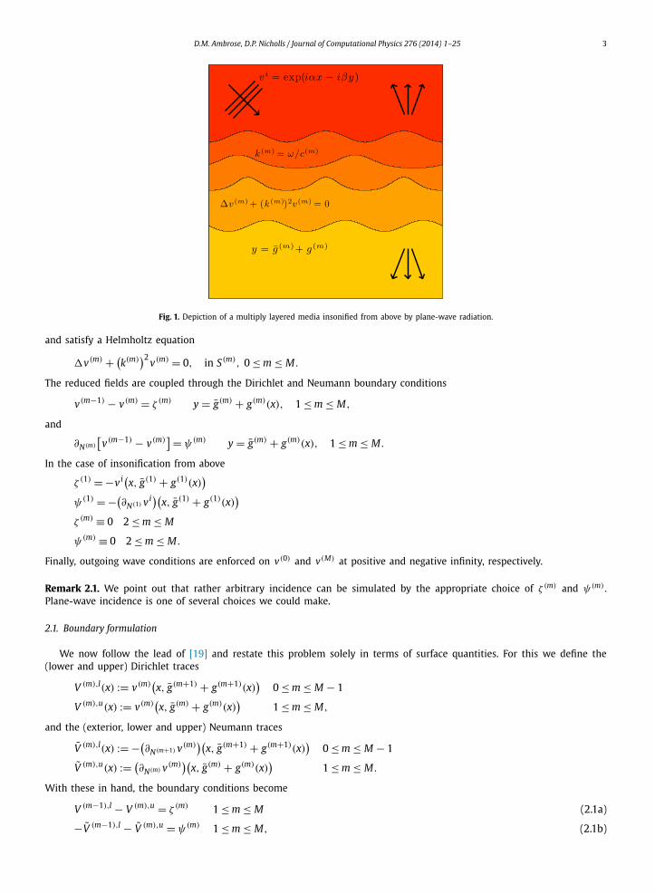
D.M. Ambrose, D.P. Nicholls / Journal of Computational Physics 276 (2014) 1–25 3

Fig. 1. Depiction of a multiply layered media insonified from above by plane-wave radiation.

and satisfy a Helmholtz equation

�v(m) + (k(m)

)2v(m) = 0, in S(m), 0 ≤ m ≤ M.

The reduced fields are coupled through the Dirichlet and Neumann boundary conditions

v(m−1) − v(m) = ζ (m) y = g(m) + g(m)(x), 1 ≤ m ≤ M,

and

∂N(m)

[v(m−1) − v(m)

] = ψ(m) y = g(m) + g(m)(x), 1 ≤ m ≤ M.

In the case of insonification from above

ζ (1) = −vi(x, g(1) + g(1)(x))

ψ(1) = −(∂N(1) vi)(x, g(1) + g(1)(x)

)ζ (m) ≡ 0 2 ≤ m ≤ M

ψ(m) ≡ 0 2 ≤ m ≤ M.

Finally, outgoing wave conditions are enforced on v(0) and v(M) at positive and negative infinity, respectively.

Remark 2.1. We point out that rather arbitrary incidence can be simulated by the appropriate choice of ζ (m) and ψ(m) . Plane-wave incidence is one of several choices we could make.

2.1. Boundary formulation

We now follow the lead of [19] and restate this problem solely in terms of surface quantities. For this we define the (lower and upper) Dirichlet traces

V (m),l(x) := v(m)(x, g(m+1) + g(m+1)(x)

)0 ≤ m ≤ M − 1

V (m),u(x) := v(m)(x, g(m) + g(m)(x)

)1 ≤ m ≤ M,

and the (exterior, lower and upper) Neumann traces

V (m),l(x) := −(∂N(m+1) v(m)

)(x, g(m+1) + g(m+1)(x)

)0 ≤ m ≤ M − 1

V (m),u(x) := (∂N(m) v(m)

)(x, g(m) + g(m)(x)

)1 ≤ m ≤ M.

With these in hand, the boundary conditions become

V (m−1),l − V (m),u = ζ (m) 1 ≤ m ≤ M (2.1a)

−V (m−1),l − V (m),u = ψ(m) 1 ≤ m ≤ M, (2.1b)

4 D.M. Ambrose, D.P. Nicholls / Journal of Computational Physics 276 (2014) 1–25

which specifies (2M) equations for (4M) unknown functions. This allows us to “eliminate” the upper traces {V (m),u, V (m),u}in favor of the lower ones {V (m),l, V (m),l} by

V (m),u = V (m−1),l − ζ (m) 1 ≤ m ≤ M (2.2a)

V (m),u = −V (m−1),l − ψ(m) 1 ≤ m ≤ M. (2.2b)

We can generate (2M) many more equations by defining the “Dirichlet–Neumann Operators” (DNOs)

G[V (0),l] := V (0),l (2.3a)

H(m)[V (m),u, V (m),l] =

(Huu(m) Hul(m)

Hlu(m) Hll(m)

)[(V (m),u

V (m),l

)]:=

(V (m),u

V (m),l

)1 ≤ m ≤ M − 1 (2.3b)

J[V (M),u] := V (M),u, (2.3c)

which relate the Dirichlet quantities, {V (m),u, V (m),l}, to the Neumann traces, {V (m),u, V (m),l}. From here we diverge from the approach of [19] which described Boundary Perturbation Methods to compute the DNOs {G, H(m), J }. For the current approach we note that in the following sections we derive integral operators A and R which relate the Dirichlet and Neumann data in the following ways

A(0)V (0),l − R(0)V (0),l = 0 (2.4a)(Auu(m) Aul(m)

Alu(m) All(m)

)(V (m),u

V (m),l

)−

(Ruu(m) Rul(m)

Rlu(m) Rll(m)

)(V (m),u

V (m),l

)=

(00

)1 ≤ m ≤ M − 1 (2.4b)

A(M)V (M),u − R(M)V (M),u = 0. (2.4c)

Now, using (2.2), we can write (2.4) as

A(0)V (0),l − R(0)V (0),l = 0(Auu(m) Aul(m)

Alu(m) All(m)

)(−V (m−1),l − ψ(m)

V (m),l

)−

(Ruu(m) Rul(m)

Rlu(m) Rll(m)

)(V (m−1),l − ζ (m)

V (m),l

)=

(00

)1 ≤ m ≤ M − 1

A(M)[−V (M−1),l − ψ(M)

] − R(M)[V (M−1),l − ζ (M)

] = 0.

Simplifying, this can be written as

MV(l) = Q (2.5)

where

M :=

⎛⎜⎜⎜⎜⎜⎜⎜⎜⎝

A(0) −R(0) 0 · · · 0−Auu(1) −Ruu(1) Aul(1) −Rul(1) · · · 0−Alu(1) −Rlu(1) All(1) −Rll(1) · · · 0

......

0 · · · −Auu(M − 1) −Ruu(M − 1) Aul(M − 1) −Rul(M − 1)

0 · · · −Alu(M − 1) −Rlu(M − 1) All(M − 1) −Rll(M − 1)

0 · · · 0 −A(M) −R(M)

⎞⎟⎟⎟⎟⎟⎟⎟⎟⎠

,

and

V(l) :=

⎛⎜⎜⎜⎜⎝

V (0),l

V (0),l

...

V (M−1),l

V (M−1),l

⎞⎟⎟⎟⎟⎠ , Q :=

⎛⎜⎜⎜⎜⎜⎜⎜⎜⎝

0Auu(1)ψ(1) − Ruu(1)ζ (1)

Alu(1)ψ(1) − Rlu(1)ζ (1)

...

Auu(M − 1)ψ(M−1) − Ruu(M − 1)ζ (M−1)

Alu(M − 1)ψ(M−1) − Rlu(M − 1)ζ (M−1)

A(M)ψ(M) − R(M)ζ (M)

⎞⎟⎟⎟⎟⎟⎟⎟⎟⎠

.

Our numerical method amounts to Nyström’s method [8] applied to MV(l) = Q and it only remains to specify the integral operators A and R , which we address in Section 3.

2.2. Special cases

A few special cases of the equations above deserve particular comment and we provide that in this section.

Single layer. The case of a single layer overlying an impenetrable material does not fit into our framework as stated, how-ever, it can be expanded to include this important configuration. Here, the reduced scattered field, v(0) , is still subject to the

D.M. Ambrose, D.P. Nicholls / Journal of Computational Physics 276 (2014) 1–25 5

Helmholtz equation, quasiperiodic boundary conditions, and the outgoing wave condition. Depending upon the properties of the impenetrable layer there is either a Dirichlet boundary condition,

V (0),l(x) = ζ (1)(x), y = g(1) + g(1)(x), (2.6)

or a Neumann boundary condition,

V (0),l(x) = ψ(1)(x), y = g(1) + g(1)(x), (2.7)

to be enforced at the interface. We can fit into the formulation given above, i.e. solving MV(l) = Q from (2.5), by making the following choices. For the Dirichlet boundary conditions, (2.6), we set

M =(

0 IA(0) −R(0)

), V(l) =

(V (0),l

V (0),l

), Q =

(ζ (1)

0

),

while for the Neumann conditions, (2.7), we equate

M =(

I 0A(0) −R(0)

), V(l) =

(V (0),l

V (0),l

), Q =

(ψ(1)

0

).

Remark 2.2. Of course these two could be further simplified to

V (0),l = ζ (1), A(0)V (0),l = R(0)ζ (1),

and

V (0),l = ψ(1), R(0)V (0),l = A(0)ψ(1),

which requires only the inversion of A(0) or R(0), rather than the full operator M.

Double layer. For the case of a single layer separating two materials which both permit propagation the boundary conditions become

V (0),l − V (1),u = ζ (1) y = g(1) + g(1)(x) (2.8a)

−V (0),l − V (1),u = ψ(1) y = g(1) + g(1)(x), (2.8b)

and we solve MV(l) = Q with

M =(

A(0) −R(0)

−A(1) −R(1)

), V(l) =

(V (0),l

V (0),l

), Q =

(0

A(1)ψ(1) − R(1)ζ (1)

).

Three layers. Finally, for a triply layered material we must satisfy the boundary conditions

V (0),l − V (1),u = ζ (1) y = g(1) + g(1)(x) (2.9a)

V (1),l − V (2),u = ζ (2) y = g(2) + g(2)(x) (2.9b)

−V (0),l − V (1),u = ψ(1) y = g(1) + g(1)(x) (2.9c)

−V (1),l − V (2),u = ψ(2) y = g(2) + g(2)(x), (2.9d)

and we solve MV(l) = Q with

M =⎛⎜⎝

A(0) −R(0) 0 0−Auu(1) −Ruu(1) Aul(1) −Rul(1)

−Alu(1) −Rlu(1) All(1) −Rll(1)

0 0 −A(2) −R(2)

⎞⎟⎠ ,

V(l) =⎛⎜⎝

V (0),l

V (0),l

V (1),l

V (1),l

⎞⎟⎠ , Q =

⎛⎜⎝

0Auu(1)ψ(1) − Ruu(1)ζ (1)

Alu(1)ψ(1) − Rlu(1)ζ (1)

A(2)ψ(2) − R(2)ζ (2)

⎞⎟⎠ .

Remark 2.3. In the case of plane-wave incidence from above we have

ζ (1) = −eiα·x−iβ(g(1)+g(1)(x)), ψ(1) = (iβ + (∇x g(1)

) · (iα))eiα·x−iβ(g(1)+g(1)(x))

which are the Dirichlet and Neumann traces of the incident field vi at the uppermost boundary y = g(1) + g(1)(x).

6 D.M. Ambrose, D.P. Nicholls / Journal of Computational Physics 276 (2014) 1–25

3. Integral equation formulation by Fokas’ method

The reformulation of the Dirichlet–Neumann Operator (DNO) problems we study here come from the remarkable proce-dure of Fokas [1,9,29,30] which, in our present context, amounts to the inspired use of the following identity which appears in [1].

Lemma 3.1. If we define

Z (k) := ∂yφ(�ψ + k2ψ

) + (�φ + k2φ

)∂yψ,

then

Z (k) = divx[

F (x)] + ∂y[

F (y) + F (k)],

where

F (x) := ∂yφ(∇xψ) + ∇xφ(∂yψ), F (y) := ∂yφ(∂yψ) − ∇xφ · (∇xψ), F (k) := k2φ ψ.

Defining the periodic domain

Ω = Ω(� + �(x), u + u(x)

) := {0 < x < d} × {� + �(x) < y < u + u(x)

},

�(x + d) = �(x), u(x + d) = u(x),

provided that φ and ψ solve the Helmholtz equation

�φ + k2φ = 0, �ψ + k2ψ = 0,

then Z (k) = 0. A (trivial) consequence of the divergence theorem gives us the following lemma.

Lemma 3.2. Suppose that G(x, y), defined on Ω , is d-periodic in the x variable, G(x + d, y) = G(x, y), where

G(x, y) = (G(x)(x, y), G(y)(x, y)

)T,

then

∫Ω

div[G]dV =d∫

0

[G(x) · (∇x�) − G(y)

]y=�+�(x) dx +

d∫0

[−G(x) · (∇xu) + G(y)]

y=u+u(x) dx.

If φ is α-quasiperiodic and ψ is (−α)-quasiperiodic, i.e.,

φ(x + d, y) = eiα·dφ(x, y), ψ(x + d, y) = e−iα·dψ(x, y),

then Lemma 3.2 tells us, with G = (F (x), F (y) + F (k))T ,

0 =∫Ω

Z (k) dV =∫

∂Ω

div[G]dV

=d∫

0

(F (x) · ∇x� − F (y) − F (k)

)y=�+�(x) dx +

d∫0

(F (x) · (−∇xu) + F (y) + F (k)

)y=u+u(x) dx,

since, in this case, the terms F (x) , F (y) , and F (k) are periodic. More specifically,

0 =d∫

0

[∂yφ(∇xψ · ∇x�) + ∇xφ · (∂yψ∇x�) − ∂yφ(∂yψ) + ∇xφ · (∇xψ) − k2φψ dx

]y=�+�(x)

+d∫

0

[∂yφ

(∇xψ · (−∇xu)) + ∇xφ · (∂yψ(−∇xu)

) + ∂yφ(∂yψ) − ∇xφ · (∇xψ) + k2φψ]

y=u+u(x) dx,

and

D.M. Ambrose, D.P. Nicholls / Journal of Computational Physics 276 (2014) 1–25 7

0 =d∫

0

[∂yψ(∇x� · ∇xφ − ∂yφ) + ∇xψ · (∇x�∂yφ + ∇xφ) − ψk2φ

]y=�+�(x) dx

+d∫

0

[∂yψ(−∇xu · ∇xφ + ∂yφ) − ∇xψ · (∇xu∂yφ + ∇xφ) + ψk2φ

]y=u+u(x) dx. (3.1)

If we define

ξ(x) := φ(x, � + �(x)

), ζ(x) := φ

(x, u + u(x)

),

then tangential derivatives are given by

∇xξ(x) := [∇xφ + ∇x�∂yφ]y=�+�(x), ∇xζ(x) := [∇xφ + ∇xu∂yφ]y=u+u(x).

Recalling the definitions of the DNOs (2.3)

L(x) := [−∂yφ + ∇x� · ∇xφ]y=�+�(x), U (x) := [∂yφ − ∇xu · ∇xφ]y=u+u(x),

Eq. (3.1) now reads

0 =d∫

0

(∂yψ)y=�+�(x)L + (∇xψ)y=�+�(x) · ∇xξ − (ψ)y=�+�(x)k2ξ dx

+d∫

0

(∂yψ)y=u+u(x)U − (∇xψ)y=u+u(x) · ∇xζ + (ψ)y=u+u(x)k2ζ dx,

or

d∫0

(∂yψ)y=u+u(x)U dx +d∫

0

(∂yψ)y=�+�(x)L dx

=d∫

0

(∇xψ)y=u+u(x) · ∇xζ dx −d∫

0

(∇xψ)y=�+�(x) · ∇xξ dx

−d∫

0

k2(ψ)y=u+u(x)ζ dx +d∫

0

k2(ψ)y=�+�(x)ξ dx. (3.2)

3.1. The top layer

For this problem we consider upward propagating, α-quasiperiodic solutions of

�φ + k2φ = 0 � + �(x) < y < u

φ = ξ y = � + �(x).

To begin, we note that the Rayleigh expansion [25] gives, for y > u, that upward propagating α-quasiperiodic solutions of the Helmholtz equation can be written as

φ(x, y) =∞∑

q=−∞ζqeiαq ·x+iβq(y−u), q = (q1,q2), (3.3)

where

αq :=(

α1 + 2πq1/d1α2 + 2πq2/d2

), βq :=

⎧⎨⎩

√k2 − |αq|2 q ∈ U

i√

|αq|2 − k2 q /∈ U,

and the set of propagating modes is specified by

U := {q

∣∣ |αq|2 < k2}.

8 D.M. Ambrose, D.P. Nicholls / Journal of Computational Physics 276 (2014) 1–25

Evaluating (3.3) at y = u delivers the (generalized) Fourier series of ζ(x),

ζ(x) =∞∑

q=−∞ζqeiαq ·x,

so that we can compute the DNO at y = u as

U = ∂yφ(x, u) =∞∑

q=−∞(iβq)ζqeiαq ·x =: (iβD)ζ. (3.4)

Proceeding, we consider an (−α)-quasiperiodic “test function”

ψ(x, y) = e−iαp ·x+imp(y−�)

with mp to be determined so that the difference between the first and the sum of the third and fifth terms in (3.2) are zero. For this we consider the quantity

R(x) := (∂yψ)y=uU − (∇xψ)y=u · ∇xζ + k2(ψ)y=uζ,

and define

E p := exp(imp(u − �)

).

It is easy to show that

R(x) = (imp)e−iαp x E p(iβD)ζ − (−iαp)e−iαp x E p · ∇xζ + k2e−iαp x E pζ

=∞∑

q=−∞

{(imp)(iβq) − (−iαp) · (iαq) + k2}E p ζqe−i(αp−αq)·x.

Integrating R over the period cell, the only non-zero term features p = q so that

d∫0

R(x)dx = |d|{(imp)(iβp) − (−iαp) · (iαp) + k2}E p ζp .

Choosing mp = βp , so that

ψ(x, y) = e−iαp x+iβp(y−�),

a “conjugated solution,” we get zero since

αp · αp + β2p = k2 �⇒ (iαp) · (iαp) + (iβp)2 + k2 = 0.

In light of these computations we now have

d∫0

(∂yψ)y=�+�(x)L dx = −d∫

0

(∇xψ)y=�+�(x) · ∇xξ dx +d∫

0

k2(ψ)y=�+�(x)ξ dx,

and, with ψ defined above,

d∫0

(iβp)eiβp�e−iαp xL dx = −d∫

0

(−iαp)eiβp�e−iαp x · ∇xξ dx +d∫

0

k2eiβp�e−iαp xξ dx.

To match with (2.3a)–(2.3c) we rename the DNO G and the interface g giving

d∫0

(iβp)eiβp ge−iαp xG dx =d∫

0

(iαp)eiβp ge−iαp x · ∇xξ dx +d∫

0

k2eiβp ge−iαp xξ dx. (3.5)

Remark 3.3. At this point one can ask how the current procedure differs from that of [1]. Here we have chosen ψ at the outset so that

∫R = 0. In contrast, [1] chose two (−α)-quasiperiodic solutions and then combined them in such a way that

these “far field” terms disappeared. We also point out that we follow the developments of [1] quite closely which is not the same as the “method” devised and analyzed in [9,29,30] (which we note does not deliver formulas for the three-dimensional problem).

D.M. Ambrose, D.P. Nicholls / Journal of Computational Physics 276 (2014) 1–25 9

3.2. The bottom layer

In a similar fashion we can consider downward propagating, α-quasiperiodic solutions of

�φ + k2φ = 0 � < y < u + u(x)

φ = ζ y = u + u(x),

and the “test function”

ψ(x, y) = e−iαp x−iβp(y−u).

With this choice of ψ the second, fourth, and sixth terms in (3.2) combine to zero and we find

d∫0

(∂yψ)y=u+u(x)U dx =d∫

0

(∇xψ)y=u+u(x) · ∇xζ dx −d∫

0

k2(ψ)y=u+u(x)ζ dx.

With ψ defined in this way we determine that

d∫0

(−iβp)e−iβp ue−iαp xU dx =d∫

0

(−iαp)e−iβp ue−iαp x · ∇xζ dx −d∫

0

k2e−iβp ue−iαp xζ dx.

Again, to match with (2.3) we rename the DNO J and the interface g giving

d∫0

(iβp)e−iβp ge−iαp x J dx =d∫

0

(iαp)e−iβp ge−iαp x · ∇xζ dx +d∫

0

k2e−iβp ge−iαp xζ dx. (3.6)

3.3. A middle layer

Finally, we consider α-quasiperiodic solutions of

�φ + k2φ = 0 � + �(x) < y < u + u(x)

φ = ξ y = � + �(x)

φ = ζ y = u + u(x),

and the “test functions”

ψ(u)(x, y) = cosh(iβp(y − �))

sinh(iβp(u − �))e−iαp x

ψ(�)(x, y) = cosh(iβp(u − y))

sinh(iβp(u − �))e−iαp x.

Defining

cop := coth(iβp(u − �)

), csp := csch

(iβp(u − �)

),

C(u) := cosh(iβpu), S(u) := sinh(iβpu),

C(�) := cosh(iβp�), S(�) := sinh(iβp�),

we can show that

ψ(u)(x, u + u) = (cop C(u) + S(u)

)e−iαp x

ψ(u)(x, � + �) = csp C(�)e−iαp x

ψ(�)(x, u + u) = csp C(u)e−iαp x

ψ(�)(x, � + �) = (cop C(�) − S(�)

)e−iαp x,

and

∂xψ(u)(x, u + u) = (−iαp)

(cop C(u) + S(u)

)e−iαp x

∂xψ(u)(x, � + �) = (−iαp) csp C(�)e−iαp x

∂xψ(�)(x, u + u) = (−iαp) csp C(u)e−iαp x

∂xψ(�)(x, � + �) = (−iαp)

(cop C(�) − S(�)

)e−iαp x,

10 D.M. Ambrose, D.P. Nicholls / Journal of Computational Physics 276 (2014) 1–25

and

∂yψ(u)(x, u + u) = (iβp)

(C(u) + cop S(u)

)e−iαp x

∂yψ(u)(x, � + �) = (iβp) csp S(�)e−iαp x

∂yψ(�)(x, u + u) = (iβp) csp S(u)e−iαp x

∂yψ(�)(x, � + �) = (−iβp)

(C(�) − cop S(�)

)e−iαp x.

From (3.2), with ψ(u) we find

d∫0

(iβp)(C(u) + cop S(u)

)e−iαp xU dx +

d∫0

(iβp) csp S(�)e−iαp xL dx

=d∫

0

(−iαp)(cop C(u) + S(u)

)e−iαp x · ∇xζ dx −

d∫0

(−iαp) csp C(�)e−iαp x · ∇xξ dx

−d∫

0

k2(cop C(u) + S(u))e−iαp xζ dx +

d∫0

k2 csp C(�)e−iαp xξ dx. (3.7)

Additionally, with ψ(�) , (3.2) delivers,

d∫0

(iβp) csp S(u)e−iαp xU dx +d∫

0

(−iβp)(C(�) − cop S(�)

)e−iαp xL dx

=d∫

0

(−iαp) csp C(u)e−iαp x · ∇xζ dx −d∫

0

(−iαp)(cop C(�) − S(�)

)e−iαp x · ∇xξ dx

−d∫

0

k2 csp C(u)e−iαp xζ dx +d∫

0

k2(cop C(�) − S(�))e−iαp xξ dx. (3.8)

3.4. Summary of formulas and zero-deformation simplifications

We point out that all of the formulas derived thus far, (3.5), (3.6), (3.7), and (3.8), can be stated generically as

Ap[V ] = R p[V ]. (3.9)

1. (Top layer) For (3.5), after dividing by (iβp),

V = G, V = ξ, Ap(g)[G] =d∫

0

eiβp ge−iαp xG(x)dx (3.10a)

R p(g)[ξ ] =d∫

0

eiβp ge−iαp x{

iαp

iβp· ∇x + k2

iβp

}ξ(x)dx. (3.10b)

2. (Bottom layer) For (3.6), after dividing by (iβp),

V = J , V = ζ, Ap(g)[ J ] =d∫

0

e−iβp ge−iαp x J (x)dx (3.11a)

R p(g)[ζ ] =d∫

0

e−iβp ge−iαp x{

iαp

iβp· ∇x + k2

iβp

}ζ(x)dx. (3.11b)

D.M. Ambrose, D.P. Nicholls / Journal of Computational Physics 276 (2014) 1–25 11

3. For (3.7) and (3.8), after dividing by (iβp),

V =(

V u

V �

)=

(UL

), V =

(V u

V �

)=

(ζ

ξ

), (3.12a)

Ap(u, �)

[(UL

)]=

d∫0

(C(u) + cop S(u) csp S(�)

− csp S(u) C(�) − cop S(�)

)(UL

)e−iαp x dx (3.12b)

R p(u, �)

[(ζ

ξ

)]=

d∫0

(− cop C(u) − S(u) csp C(�)

csp C(u) − cop C(�) + S(�)

)

×{

iαp

iβp· ∇x + k2

iβp

}(ζ

ξ

)e−iαp x dx. (3.12c)

In the class of flat interfaces (g ≡ 0, u ≡ 0, � ≡ 0) we have

1. (Top layer)

Ap(0)[G] =d∫

0

e−iαp xG(x)dx

R p(0)[ξ ] =d∫

0

e−iαp x{

iαp

iβp· ∇x + k2

iβp

}ξ(x)dx.

2. (Bottom layer)

Ap(0)[ J ] =d∫

0

e−iαp x J (x)dx

R p(0)[ζ ] =d∫

0

e−iαp x{

iαp

iβp· ∇x + k2

iβp

}ζ(x)dx.

3. (Middle layer)

Ap(0,0)

[(UL

)]=

d∫0

(1 00 1

)(UL

)e−iαp x dx

R p(0,0)

[(ζ

ξ

)]=

d∫0

(− cop csp

csp − cop

){iαp

iβp· ∇x + k2

iβp

}(ζ

ξ

)e−iαp x dx.

Recognizing the Fourier transform

ψp = F [ψ] =d∫

0

e−iαp xψ(x)dx,

and using the fact that (iαp) · (iαp) + k2 = −(iβp)2 we find

1. (Top layer)

Ap(0)[G] = G p

R p(0)[ξ ] ={

iαp

iβp· (iαp) + k2

iβp

}ξp = −(iβp)ξp .

12 D.M. Ambrose, D.P. Nicholls / Journal of Computational Physics 276 (2014) 1–25

2. (Bottom layer)

Ap(0)[ J ] = J p

R p(0)[ζ ] ={

iαp

iβp· (iαp) + k2

iβp

}ζp = −(iβp)ζp .

3. (Middle layer)

Ap(0,0)

[(UL

)]=

(1 00 1

)(U p

Lp

)

R p(0,0)

[(ζ

ξ

)]=

(− cop csp

csp − cop

){iαp

iβp· (iαp) + k2

iβp

}(ζp

ξp

)

=(− cop csp

csp − cop

)(−iβp)

(ζp

ξp

),

and discover the classical results

G p = −(iβp)ξp, J p = −(iβp)ζp,(U p

Lp

)= (iβp)

(cop − csp

− csp cop

)(ζp

ξp

).

We close by pointing out that (3.9) specifies equations for the Fourier coefficients of V and V rather than the functions themselves. To specify equations for the latter, as a function of the variable x, we simply invert the Fourier transform, e.g.,

A[V ] = R[V ], (3.13)

where

A = 1

|d|∞∑

p=−∞Apeiαp ·x, R = 1

|d|∞∑

p=−∞R peiαp ·x.

In our simulations below we apply Nyström’s method [8] to (3.13) instead of (3.9).

Remark 3.4. Due to the smoothness of solutions in the presence of smooth interfaces, we choose equally spaced gridpoints in our Nyström approach resulting in the trapezoidal rule. We remark that Fast Fourier Transforms (FFTs) [10] could be used as a fast inversion strategy for this flat-interface configuration. However, such an approach cannot be used for general deformations.

4. Computing far-field information: the efficiencies

In many situations it is insufficient to know the scattered fields at the layer interfaces, for instance when “far field” data is required. In periodic layered media scattering, such information is encoded in the efficiencies [25] and in this section we describe how the Fokas formalism can be used to derive equations for these from the unknowns of the problem.

To begin we once again use the Rayleigh expansions which state that above the structure the scattered field can be expressed as

v(0)(x, y) =∞∑

p=−∞B(0)

p eiαp ·x+iβ(0)p y,

while below the structure

v(M)(x, y) =∞∑

p=−∞B(M)

p eiαp ·x−iβ(M)p y .

The upper and lower efficiencies (together with the set of propagating modes) are defined by

e(0)p := β

(0)p

β

∣∣B(0)p

∣∣2, p ∈ U (0) = {

p∣∣ |αp|2 <

(k(0)

)2}

e(M)p := β

(M)p ∣∣B(M)

p

∣∣2, p ∈ U (M) = {

p∣∣ |αp|2 <

(k(M)

)2}.

β

D.M. Ambrose, D.P. Nicholls / Journal of Computational Physics 276 (2014) 1–25 13

There is a principle of conservation of energy for lossless media which states that∑p∈U (0)

e(0)p +

∑p∈U (M)

e(M)p = 1,

which gives a diagnostic of convergence, the “energy defect”

δ := 1 −∑

p∈U (0)

e(0)p −

∑p∈U (M)

e(M)p . (4.1)

We now seek formulae to recover the {B(0)p , B(M)

p } from the Dirichlet and Neumann traces which we can compute from our algorithm. We begin with the uppermost layer and, for simplicity, drop the zero-superscript. Consider the hyperplane y = u (u > g(1) + g(1)(x)) and the Dirichlet trace

ζ(x) := v(x, u) =∞∑

p=−∞B peiαp ·x+iβp u.

Therefore, if we can recover ζ(x) then

∞∑p=−∞

ζpeiαp ·x = ζ(x) = v(x, u) =∞∑

p=−∞B peiαp ·x+iβp u,

which gives

B p = ζpe−iβp u .

Once again, we work with (3.2) and recall that in this flat-interface case, cf. (3.4),

U = (iβD)ζ.

We suppose that we know the following data at y = � + �(x):

ξ(x), ∇xξ(x), L(x),

and, in the same spirit as Section 3.1, seek a relation between these and ζ . Of course, if we utilize the same function ψ then the data at y = u disappear entirely, however, if we change this slightly (effectively a change of sign in the y-dependence) to

ψ(x, y) = e−iαp ·x+iβp(u−y),

we can realize a convenient formula for ζp . We insert this choice into (3.2) to deliver

d∫0

(−iβp)e−iαp xU dx +d∫

0

(−iβp)eiβp(u−�)e−iβp�(x)e−iαp xL dx

=d∫

0

(−iαp)e−iαp x · ∇xζ dx −d∫

0

(−iαp)eiβp(u−�)e−iβp�(x)e−iαp x · ∇xξ dx

−d∫

0

k2e−iαp xζ dx +d∫

0

k2eiβp(u−�)e−iβp�(x)e−iαp xξ dx.

Moving the data at y = u to the left and terms evaluated at y = � + �(x) to the right, and, once again, recognizing the Fourier transforms, we find[

(−iβp)(iβp) + (iαp) · (iαp) + k2]ζp = Q p,

where

Q (x) = eiβp(u−�)e−iβp�(x){(iβp)L(x) + (iαp) · ∇xξ(x) + k2ξ(x)}.

We can simplify this to

ζp = Q p

[−2(iβ )2] ,

p

14 D.M. Ambrose, D.P. Nicholls / Journal of Computational Physics 276 (2014) 1–25

which delivers

B p = −e−iβp u Q p

2(iβp)2.

In the simple case of a flat lower interface, �(x) ≡ 0, we find

Q (x) = eiβp(u−�){(iβp)L(x) + (iαp) · ∇xξ(x) + k2ξ(x)

},

so

Q p = eiβp(u−�){(iβp)L p + (iαp) · (iαp)ξp + k2ξp

} = eiβp(u−�){−2(iβp)2},

and

B p = −e−iβp u Q p

2(iβp)2= −e−iβp u 1

2(iβp)2eiβp(u−�)

(−2(iβp)2) = e−iβp �.

For the lower-layer Rayleigh coefficients we can proceed in much the same way. Here we drop the (M)-superscript and denote the Rayleigh coefficients by C p . Consider y = � (� < gM + gM(x)) and the Dirichlet trace

ξ(x) := v(x, �) =∞∑

p=−∞C peiαp ·x−iβp �.

Therefore, if we can recover ξ(x) then

∞∑p=−∞

ξpeiαp ·x = ξ(x) = v(x, �) =∞∑

p=−∞C peiαp ·x−iβp �,

which gives

C p = ξpeiβp �.

If we now follow Section 3.2 with �(x) ≡ 0 (noting that L = −(−iβD) = (iβD)), but now choose

ψ(x, y) = e−iαp x+iβp(y−�)

then (3.2) gives

d∫0

(iβp)eiβp(u−�)eiβp u(x)e−iαp xU dx +d∫

0

(iβp)e−iαp xL dx

=d∫

0

(−iαp)eiβp(u−�)eiβp u(x)e−iαp x · ∇xζ dx −d∫

0

(−iαp)e−iαp x · ∇xξ dx

−d∫

0

k2eiβp(u−�)eiβp u(x)e−iαp xζ dx +d∫

0

k2e−iαp xξ dx.

Now, moving the data at y = � to the left and the terms at y = u + u(x) to the right, we recognize the Fourier transform[(iβp)(iβp) − (iαp) · (iαp) − k2]ξp = R p,

where

R(x) = eiβp(u−�)eiβp u(x){−(iβp)U (x) − (iαp) · ∇xζ(x) − k2ζ(x)}.

We can simplify this to

ξp = R p

[2(iβp)2] ,

which delivers

C p = eiβp � R p

2(iβ )2.

p

D.M. Ambrose, D.P. Nicholls / Journal of Computational Physics 276 (2014) 1–25 15

In the simple case of a flat upper interface, u(x) ≡ 0, we find

R(x) = eiβp(u−�){−(iβp)U (x) − (iαp) · ∇xζ(x) − k2ζ(x)

},

so, since U = −iβDζ ,

R p = eiβp(u−�){(iβp)U p − (iαp) · (iαp)ζp + k2ζp

} = eiβp(u−�){−2(iβp)2},

and

C p = eiβp � R p

2(iβp)2= e−iβp � 1

2(iβp)2eiβp(u−�)

(−2(iβp)2) = −e−iβp u .

5. Numerical results

We now present detailed descriptions of numerical simulations conducted with our new approach. As we mentioned above, the scheme is simply Nyström’s Method applied to each of the Integral Equations (3.13) which appear in the full layered-medium system (2.5).

5.1. Exact solutions

For non-trivial interface shapes there are no known exact solutions for plane-wave incidence. To establish convergence of our algorithm we utilize the following principle: In building a numerical solver for a homogeneous PDE and boundary conditions:

Lu = 0 in Ω

Bu = 0 at ∂Ω,

it is often just as easy to construct an algorithm for the corresponding inhomogeneous problem:

Lu = R in Ω

Bu = Q at ∂Ω.

Selecting an arbitrary function w , we can compute

Rw := Lw, Qw := Bw,

and now have an exact solution to the problem

Lu = Rw in Ω

Bu = Qw at ∂Ω,

namely u = w . In this way we can test our inhomogeneous solver for which the homogeneous solver is a special case. However, one should select w which have the same “behavior” as solutions u of the homogeneous problem and here we specify w such that Rw ≡ 0. We point out though that our exact solution does not correspond to plane-wave incidence (but rather to plane-wave reflection).

To be more specific, consider the functions

v(m)r (x, y) = A(m)ei(αr ·x+β

(m)r y) + B(m)ei(αr ·x−β

(m)r y) (5.1)

with A(M) = B(0) = 0. These are outgoing, α-quasiperiodic solutions of the Helmholtz equation, so that Rw ≡ 0 in the notation above. However, the boundary conditions satisfied by these functions are not those satisfied by an incident plane wave. With the construction of the Qw in mind we compute the surface data

ζ (m) := v(m−1)r − v(m)

r y = g(m) + g(m)(x), 1 ≤ m ≤ M

ψ(m) := ∂N(m)

[v(m−1)

r − v(m)r

]y = g(m) + g(m)(x), 1 ≤ m ≤ M.

This is a family of exact solutions against which to test our numerical algorithm for any choice of deformations {g(1), . . . , g(M)}.

16 D.M. Ambrose, D.P. Nicholls / Journal of Computational Physics 276 (2014) 1–25

5.2. Numerical implementation and error measurement

We utilize Nyström’s Method [8] to simulate the Integral Equations (3.13) as they appear in (2.5). In this setting this amounts to enforcing these equations at N = (N1, N2) equally spaced gridpoints, x j = (x1, j1 , x2, j2 ), on the period cell [0, d1] × [0, d2], with unknowns being the functions {V (m),l, V (m),l} at these same gridpoints x j . The resulting linear sys-tem was solved directly in time O((MNx)

3) which sufficed for the purposes of the simulations conducted here.With these approximations in hand, we can make any number of error measurements versus the exact solutions (5.1).

For definiteness we choose to measure the defect in the lower Dirichlet and Neumann traces, and for the results described in Section 5.3 we measure

εrel := sup0≤m≤M−1

{ |V (m),lr − V (m),l,N

r |L∞

|V (m),lr |L∞

,|V (m),l

r − V (m),l,Nr |L∞

|V (m),lr |L∞

}. (5.2)

In this, e.g.,

V (m),lr := v(m)

r(x, g(m+1) + g(m+1)(x)

), V (m),l,N

r :=N∑

n=0

V (m),lr,n (x)εn,

the exact and approximate solutions, respectively.

Remark 5.1. The applicability of our method is determined by the mapping properties of M(g) and Q(g), more specifi-cally M(g)−1. Theoretical results along these lines are the subject of our current investigations, but we expect that these properties deteriorate as g becomes more rough (down to Lipschitz [7,12]) and as k(m) increases.

5.3. Convergence studies

For our convergence studies we follow the lead of [19] and select configurations quite close to the ones considered there. To begin we consider the two-dimensional and 2π -periodic case where the profiles are independent of the x2-variable. We will consider the fully three-dimensional case shortly. Recall the three profiles introduced in [21] for precisely this purpose: The sinusoid

f s(x) = cos(x), (5.3a)

the “rough” (C4 but not C5) profile

fr(x) = (2 × 10−4){x4(2π − x)4 − 128π8

315

}, (5.3b)

and the Lipschitz boundary

f L(x) ={−(2/π)x + 1, 0 ≤ x ≤ π

(2/π)x − 3, π ≤ x ≤ 2π. (5.3c)

We point out that all three profiles have zero mean, approximate amplitude 2, and maximum slope of roughly 1. The Fourier series representations of fr and f L are listed in [21] and in order to minimize aliasing errors we approximate these by their truncated P -term Fourier series, fr,P and f L,P .

We begin with two three-layer configurations:

1. (Two smooth interfaces, Fig. 2.) Physical and numerical parameters:

α = 0.1, β(0) = 1.1, β(1) = 2.2, β(2) = 3.3,

g(1)(x) = ε f s(x), g(2)(x) = ε f s(x), ε = 0.01, d = 2π,

N = 10, . . . ,30. (5.4)

2. (Rough and Lipschitz interfaces, Fig. 3.) Physical and numerical parameters:

α = 0.1, β(0) = 1.1, β(1) = 2.2, β(2) = 3.3,

g(1)(x) = ε fr,40(x), g(2)(x) = ε f L,40(x), ε = 0.03, d = 2π,

N = 80, . . . ,320. (5.5)

D.M. Ambrose, D.P. Nicholls / Journal of Computational Physics 276 (2014) 1–25 17

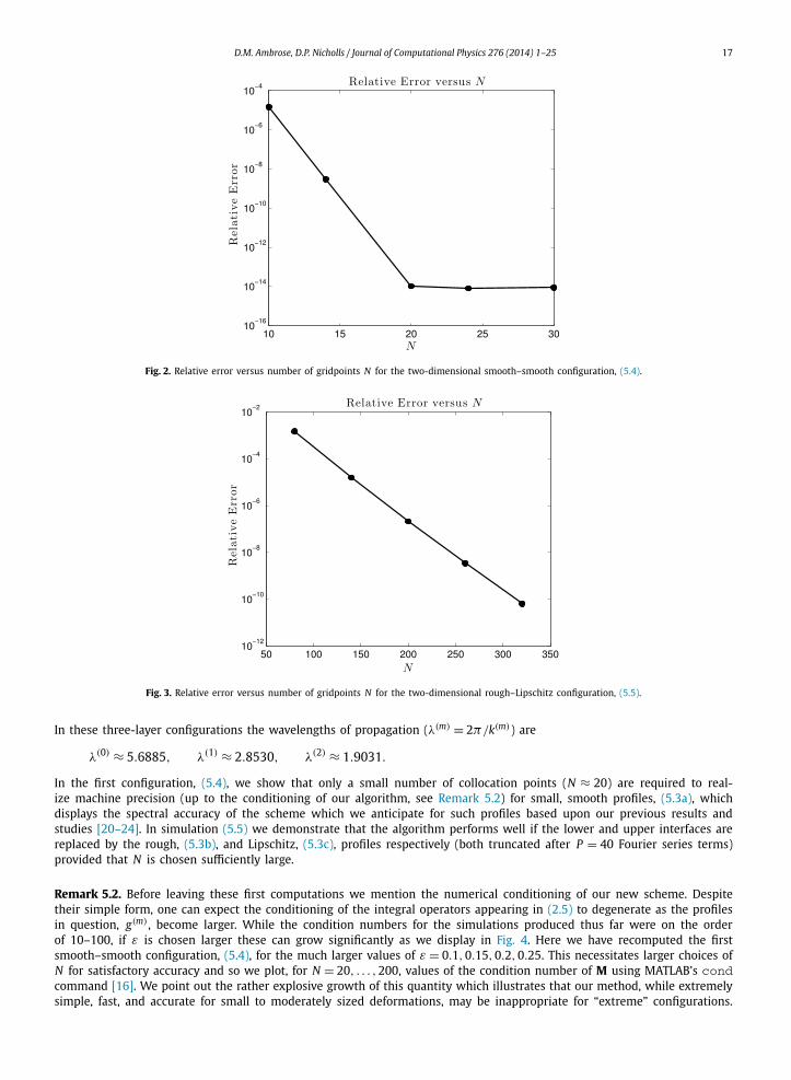
Fig. 2. Relative error versus number of gridpoints N for the two-dimensional smooth–smooth configuration, (5.4).

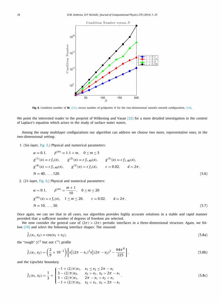
Fig. 3. Relative error versus number of gridpoints N for the two-dimensional rough–Lipschitz configuration, (5.5).

In these three-layer configurations the wavelengths of propagation (λ(m) = 2π/k(m)) are

λ(0) ≈ 5.6885, λ(1) ≈ 2.8530, λ(2) ≈ 1.9031.

In the first configuration, (5.4), we show that only a small number of collocation points (N ≈ 20) are required to real-ize machine precision (up to the conditioning of our algorithm, see Remark 5.2) for small, smooth profiles, (5.3a), which displays the spectral accuracy of the scheme which we anticipate for such profiles based upon our previous results and studies [20–24]. In simulation (5.5) we demonstrate that the algorithm performs well if the lower and upper interfaces are replaced by the rough, (5.3b), and Lipschitz, (5.3c), profiles respectively (both truncated after P = 40 Fourier series terms) provided that N is chosen sufficiently large.

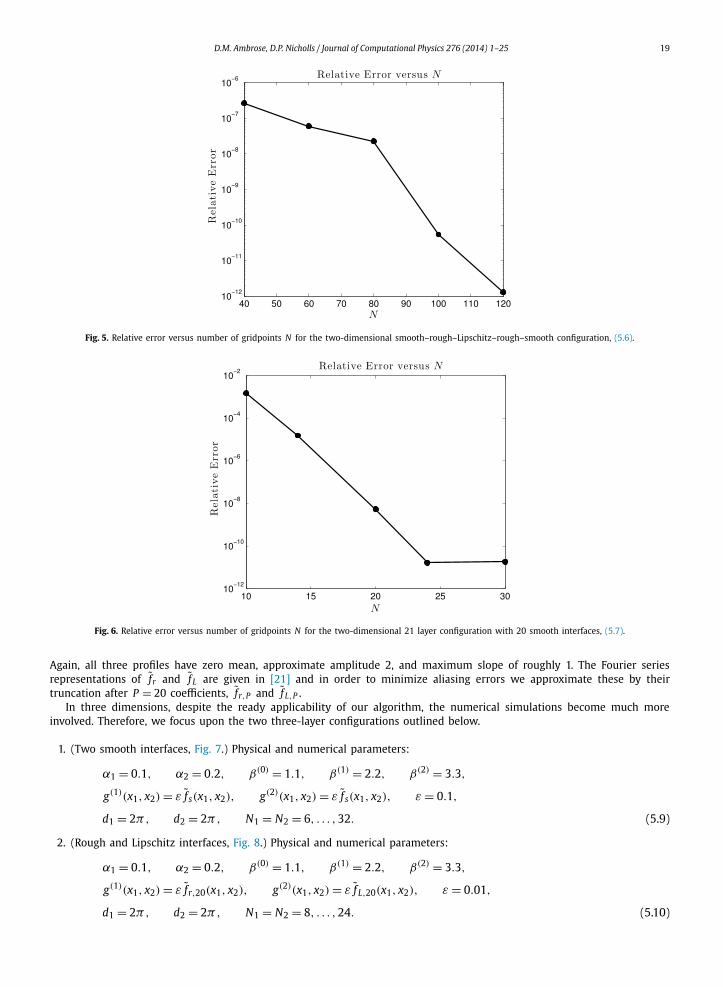
Remark 5.2. Before leaving these first computations we mention the numerical conditioning of our new scheme. Despite their simple form, one can expect the conditioning of the integral operators appearing in (2.5) to degenerate as the profiles in question, g(m) , become larger. While the condition numbers for the simulations produced thus far were on the order of 10–100, if ε is chosen larger these can grow significantly as we display in Fig. 4. Here we have recomputed the first smooth–smooth configuration, (5.4), for the much larger values of ε = 0.1, 0.15, 0.2, 0.25. This necessitates larger choices of N for satisfactory accuracy and so we plot, for N = 20, . . . , 200, values of the condition number of M using MATLAB’s condcommand [16]. We point out the rather explosive growth of this quantity which illustrates that our method, while extremely simple, fast, and accurate for small to moderately sized deformations, may be inappropriate for “extreme” configurations.

18 D.M. Ambrose, D.P. Nicholls / Journal of Computational Physics 276 (2014) 1–25

Fig. 4. Condition number of M, (2.5), versus number of gridpoints N for the two-dimensional smooth–smooth configuration, (5.4).

We point the interested reader to the preprint of Wilkening and Vasan [32] for a more detailed investigation in the context of Laplace’s equation which arises in the study of surface water waves.

Among the many multilayer configurations our algorithm can address we choose two more, representative ones, in the two-dimensional setting:

1. (Six-layer, Fig. 5.) Physical and numerical parameters:

α = 0.1, β(m) = 1.1 + m, 0 ≤ m ≤ 5

g(1)(x) = ε f s(x), g(2)(x) = ε fr,40(x), g(3)(x) = ε f L,40(x),

g(4)(x) = ε fr,40(x), g(5)(x) = ε f s(x), ε = 0.02, d = 2π,

N = 40, . . . ,120. (5.6)

2. (21-layer, Fig. 6.) Physical and numerical parameters:

α = 0.1, β(m) = m + 1

10, 0 ≤ m ≤ 20

g(m)(x) = ε f s(x), 1 ≤ m ≤ 20, ε = 0.02, d = 2π,

N = 10, . . . ,30. (5.7)

Once again, we can see that in all cases, our algorithm provides highly accurate solutions in a stable and rapid manner provided that a sufficient number of degrees of freedom are selected.

We now consider the general case of (2π) × (2π) periodic interfaces in a three-dimensional structure. Again, we fol-low [19] and select the following interface shapes: The sinusoid

f s(x1, x2) = cos(x1 + x2), (5.8a)

the “rough” (C2 but not C3) profile

f r(x1, x2) =(

2

9× 10−3

){x2

1(2π − x1)2x2

2(2π − x2)2 − 64π8

225

}, (5.8b)

and the Lipschitz boundary

f L(x1, x2) = 1

3+

⎧⎪⎨⎪⎩

−1 + (2/π)x1, x1 ≤ x2 ≤ 2π − x13 − (2/π)x2, x2 > x1, x2 > 2π − x13 − (2/π)x1, 2π − x1 < x2 < x1

. (5.8c)

−1 + (2/π)x2, x2 < x1, x2 < 2π − x1

D.M. Ambrose, D.P. Nicholls / Journal of Computational Physics 276 (2014) 1–25 19

Fig. 5. Relative error versus number of gridpoints N for the two-dimensional smooth–rough–Lipschitz–rough–smooth configuration, (5.6).

Fig. 6. Relative error versus number of gridpoints N for the two-dimensional 21 layer configuration with 20 smooth interfaces, (5.7).

Again, all three profiles have zero mean, approximate amplitude 2, and maximum slope of roughly 1. The Fourier series representations of f r and f L are given in [21] and in order to minimize aliasing errors we approximate these by their truncation after P = 20 coefficients, f r,P and f L,P .

In three dimensions, despite the ready applicability of our algorithm, the numerical simulations become much more involved. Therefore, we focus upon the two three-layer configurations outlined below.

1. (Two smooth interfaces, Fig. 7.) Physical and numerical parameters:

α1 = 0.1, α2 = 0.2, β(0) = 1.1, β(1) = 2.2, β(2) = 3.3,

g(1)(x1, x2) = ε f s(x1, x2), g(2)(x1, x2) = ε f s(x1, x2), ε = 0.1,

d1 = 2π, d2 = 2π, N1 = N2 = 6, . . . ,32. (5.9)

2. (Rough and Lipschitz interfaces, Fig. 8.) Physical and numerical parameters:

α1 = 0.1, α2 = 0.2, β(0) = 1.1, β(1) = 2.2, β(2) = 3.3,

g(1)(x1, x2) = ε f r,20(x1, x2), g(2)(x1, x2) = ε f L,20(x1, x2), ε = 0.01,

d1 = 2π, d2 = 2π, N1 = N2 = 8, . . . ,24. (5.10)

20 D.M. Ambrose, D.P. Nicholls / Journal of Computational Physics 276 (2014) 1–25

Fig. 7. Relative error versus number of gridpoints N for the three-dimensional smooth–smooth configuration, (5.9).

Fig. 8. Relative error versus number of gridpoints N for the three-dimensional rough–Lipschitz configuration, (5.10).

Again, our algorithm produces highly accurate results in a stable and reliable manner. The behavior is independent of interface shape provided that a sufficient number of collocation points are used.

5.4. Layered medium simulations

Having verified the validity of our codes, we demonstrate the utility of our approach by simulating plane-wave scattering from all of the configurations described in the previous section. Recall, in two dimensions this included two two-layer (5.4)and (5.5), and two multiple-layer problems (5.6) and (5.7); while in three dimensions this featured two two-layer scenar-ios (5.9) and (5.10). For this there is no exact solution for comparison so we resort to our diagnostic of energy defect (4.1).

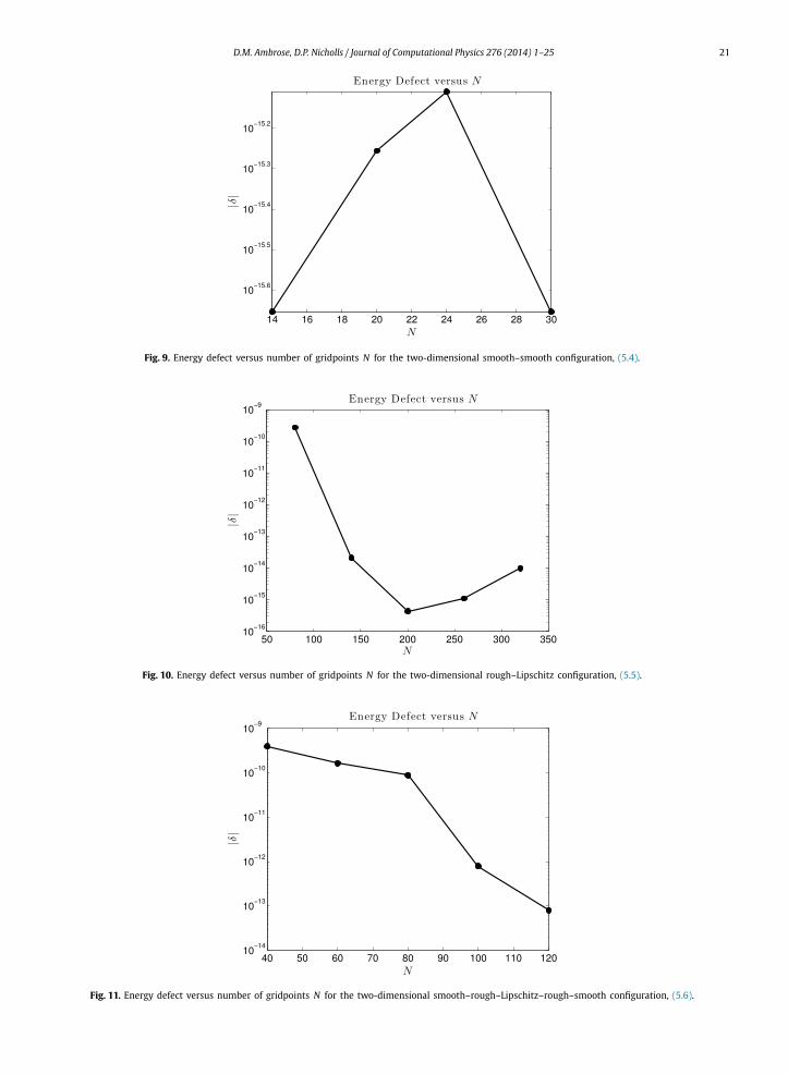
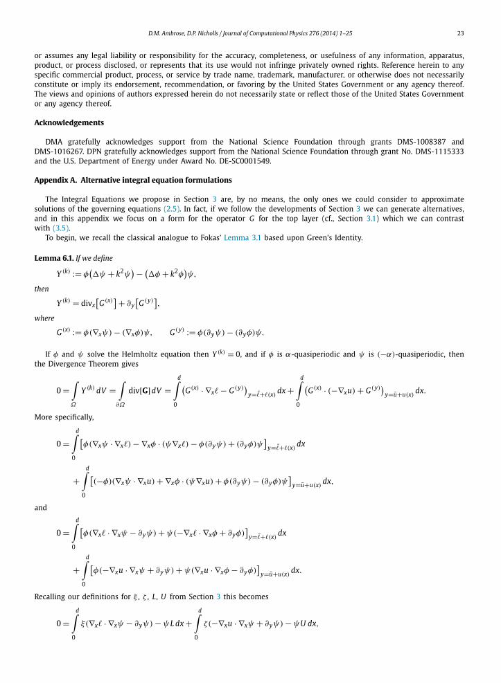
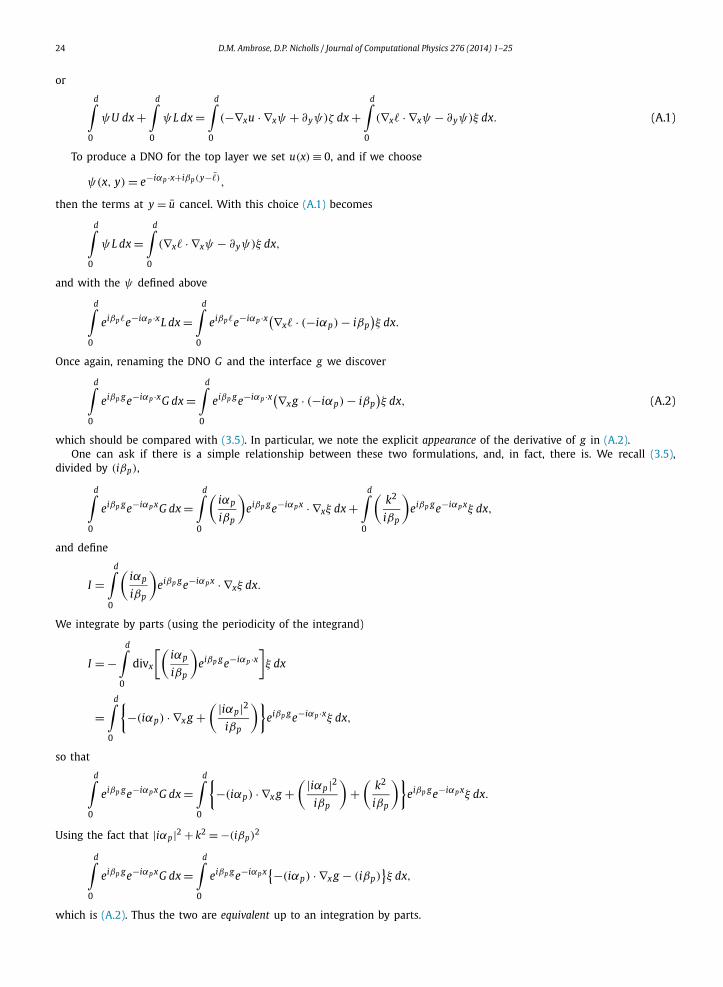
We observe in Fig. 9 that we achieve full double precision accuracy with our coarsest discretization for the smooth–smooth configuration, (5.4), while in Fig. 10 we show that the same can be realized with N ≈ 200 for the rough–Lipschitz problem, (5.5). The same generic behavior is noticed for the six-layer configuration, (5.6), and the 21 layer device, (5.7), which are displayed in Figs. 11 and 12, respectively. Finally, we display three-dimensional results corresponding to the two-layer problems, (5.9) and (5.10), and the quantitative results are given in Figs. 13 and 14, respectively.

6. Disclaimer

This report was prepared as an account of work sponsored by an agency of the United States Government. Neither the United States Government nor any agency thereof, nor any of their employees, make any warranty, express or implied,

D.M. Ambrose, D.P. Nicholls / Journal of Computational Physics 276 (2014) 1–25 21

Fig. 9. Energy defect versus number of gridpoints N for the two-dimensional smooth–smooth configuration, (5.4).

Fig. 10. Energy defect versus number of gridpoints N for the two-dimensional rough–Lipschitz configuration, (5.5).

Fig. 11. Energy defect versus number of gridpoints N for the two-dimensional smooth–rough–Lipschitz–rough–smooth configuration, (5.6).

22 D.M. Ambrose, D.P. Nicholls / Journal of Computational Physics 276 (2014) 1–25

Fig. 12. Energy defect versus number of gridpoints N for the two-dimensional 21 layer configuration with 20 smooth interfaces, (5.7).

Fig. 13. Energy defect versus number of gridpoints N for the three-dimensional smooth–smooth configuration, (5.9).

Fig. 14. Energy defect versus number of gridpoints N for the three-dimensional rough–Lipschitz configuration, (5.10).

D.M. Ambrose, D.P. Nicholls / Journal of Computational Physics 276 (2014) 1–25 23

or assumes any legal liability or responsibility for the accuracy, completeness, or usefulness of any information, apparatus, product, or process disclosed, or represents that its use would not infringe privately owned rights. Reference herein to any specific commercial product, process, or service by trade name, trademark, manufacturer, or otherwise does not necessarily constitute or imply its endorsement, recommendation, or favoring by the United States Government or any agency thereof. The views and opinions of authors expressed herein do not necessarily state or reflect those of the United States Government or any agency thereof.

Acknowledgements

DMA gratefully acknowledges support from the National Science Foundation through grants DMS-1008387 and DMS-1016267. DPN gratefully acknowledges support from the National Science Foundation through grant No. DMS-1115333 and the U.S. Department of Energy under Award No. DE-SC0001549.

Appendix A. Alternative integral equation formulations

The Integral Equations we propose in Section 3 are, by no means, the only ones we could consider to approximate solutions of the governing equations (2.5). In fact, if we follow the developments of Section 3 we can generate alternatives, and in this appendix we focus on a form for the operator G for the top layer (cf., Section 3.1) which we can contrast with (3.5).

To begin, we recall the classical analogue to Fokas’ Lemma 3.1 based upon Green’s Identity.

Lemma 6.1. If we define

Y (k) := φ(�ψ + k2ψ

) − (�φ + k2φ

)ψ,

then

Y (k) = divx[G(x)] + ∂y

[G(y)

],

where

G(x) := φ(∇xψ) − (∇xφ)ψ, G(y) := φ(∂yψ) − (∂yφ)ψ.

If φ and ψ solve the Helmholtz equation then Y (k) = 0, and if φ is α-quasiperiodic and ψ is (−α)-quasiperiodic, then the Divergence Theorem gives

0 =∫Ω

Y (k) dV =∫

∂Ω

div[G]dV =d∫

0

(G(x) · ∇x� − G(y)

)y=�+�(x) dx +

d∫0

(G(x) · (−∇xu) + G(y)

)y=u+u(x) dx.

More specifically,

0 =d∫

0

[φ(∇xψ · ∇x�) − ∇xφ · (ψ∇x�) − φ(∂yψ) + (∂yφ)ψ

]y=�+�(x) dx

+d∫

0

[(−φ)(∇xψ · ∇xu) + ∇xφ · (ψ∇xu) + φ(∂yψ) − (∂yφ)ψ

]y=u+u(x) dx,

and

0 =d∫

0

[φ(∇x� · ∇xψ − ∂yψ) + ψ(−∇x� · ∇xφ + ∂yφ)

]y=�+�(x) dx

+d∫

0

[φ(−∇xu · ∇xψ + ∂yψ) + ψ(∇xu · ∇xφ − ∂yφ)

]y=u+u(x) dx.

Recalling our definitions for ξ , ζ , L, U from Section 3 this becomes

0 =d∫ξ(∇x� · ∇xψ − ∂yψ) − ψ L dx +

d∫ζ(−∇xu · ∇xψ + ∂yψ) − ψU dx,

0 0

24 D.M. Ambrose, D.P. Nicholls / Journal of Computational Physics 276 (2014) 1–25

or

d∫0

ψU dx +d∫

0

ψ L dx =d∫

0

(−∇xu · ∇xψ + ∂yψ)ζ dx +d∫

0

(∇x� · ∇xψ − ∂yψ)ξ dx. (A.1)

To produce a DNO for the top layer we set u(x) ≡ 0, and if we choose

ψ(x, y) = e−iαp ·x+iβp(y−�),

then the terms at y = u cancel. With this choice (A.1) becomes

d∫0

ψ L dx =d∫

0

(∇x� · ∇xψ − ∂yψ)ξ dx,

and with the ψ defined above

d∫0

eiβp�e−iαp ·xL dx =d∫

0

eiβp�e−iαp ·x(∇x� · (−iαp) − iβp)ξ dx.

Once again, renaming the DNO G and the interface g we discover

d∫0

eiβp ge−iαp ·xG dx =d∫

0

eiβp ge−iαp ·x(∇x g · (−iαp) − iβp)ξ dx, (A.2)

which should be compared with (3.5). In particular, we note the explicit appearance of the derivative of g in (A.2).One can ask if there is a simple relationship between these two formulations, and, in fact, there is. We recall (3.5),

divided by (iβp),

d∫0

eiβp ge−iαp xG dx =d∫

0

(iαp

iβp

)eiβp ge−iαp x · ∇xξ dx +

d∫0

(k2

iβp

)eiβp ge−iαp xξ dx,

and define

I =d∫

0

(iαp

iβp

)eiβp ge−iαp x · ∇xξ dx.

We integrate by parts (using the periodicity of the integrand)

I = −d∫

0

divx

[(iαp

iβp

)eiβp ge−iαp ·x

]ξ dx

=d∫

0

{−(iαp) · ∇x g +

( |iαp|2iβp

)}eiβp ge−iαp ·xξ dx,

so that

d∫0

eiβp ge−iαp xG dx =d∫

0

{−(iαp) · ∇x g +

( |iαp|2iβp

)+

(k2

iβp

)}eiβp ge−iαp xξ dx.

Using the fact that |iαp |2 + k2 = −(iβp)2

d∫0

eiβp ge−iαp xG dx =d∫

0

eiβp ge−iαp x{−(iαp) · ∇x g − (iβp)}ξ dx,

which is (A.2). Thus the two are equivalent up to an integration by parts.

D.M. Ambrose, D.P. Nicholls / Journal of Computational Physics 276 (2014) 1–25 25

References

[1] M.J. Ablowitz, A.S. Fokas, Z.H. Musslimani, On a new non-local formulation of water waves, J. Fluid Mech. 562 (2006) 313–343.[2] L.M. Brekhovskikh, Y.P. Lysanov, Fundamentals of Ocean Acoustics, Springer-Verlag, Berlin, 1982.[3] Oscar P. Bruno, Fernando Reitich, Numerical solution of diffraction problems: a method of variation of boundaries, J. Opt. Soc. Am. A 10 (6) (1993)

1168–1175.[4] Oscar P. Bruno, Fernando Reitich, Numerical solution of diffraction problems: a method of variation of boundaries. II. Finitely conducting gratings, Padé

approximants, and singularities, J. Opt. Soc. Am. A 10 (11) (1993) 2307–2316.[5] Oscar P. Bruno, Fernando Reitich, Numerical solution of diffraction problems: a method of variation of boundaries. III. Doubly periodic gratings, J. Opt.

Soc. Am. A 10 (12) (1993) 2551–2562.[6] R. Coifman, M. Goldberg, T. Hrycak, M. Israeli, V. Rokhlin, An improved operator expansion algorithm for direct and inverse scattering computations,

Waves Random Media 9 (3) (1999) 441–457.[7] R. Coifman, Y. Meyer, Nonlinear harmonic analysis and analytic dependence, in: Pseudodifferential Operators and Applications, Notre Dame, IN, 1984,

Am. Math. Soc., 1985, pp. 71–78.[8] David Colton, Rainer Kress, Inverse Acoustic and Electromagnetic Scattering Theory, 2nd edition, Springer-Verlag, Berlin, 1998.[9] Athanassios S. Fokas, A Unified Approach to Boundary Value Problems, CBMS-NSF Reg. Conf. Ser. Appl. Math., vol. 78, Society for Industrial and Applied

Mathematics (SIAM), Philadelphia, PA, 2008.[10] David Gottlieb, Steven A. Orszag, Numerical Analysis of Spectral Methods: Theory and Applications, CBMS-NSF Reg. Conf. Ser. Appl. Math., vol. 26,

Society for Industrial and Applied Mathematics, Philadelphia, PA, 1977.[11] L. Greengard, V. Rokhlin, A fast algorithm for particle simulations, J. Comput. Phys. 73 (2) (1987) 325–348.[12] Bei Hu, David P. Nicholls, Analyticity of Dirichlet–Neumann operators on Hölder and Lipschitz domains, SIAM J. Math. Anal. 37 (1) (2005) 302–320.[13] D. Komatitsch, J. Tromp, Spectral-element simulations of global seismic wave propagation – I. Validation, Geophys. J. Int. 149 (2) (2002) 390–412.[14] Alison Malcolm, David P. Nicholls, A boundary perturbation method for recovering interface shapes in layered media, Inverse Probl. 27 (9) (2011)

095009.[15] Alison Malcolm, David P. Nicholls, A field expansions method for scattering by periodic multilayered media, J. Acoust. Soc. Am. 129 (4) (2011)

1783–1793.[16] MATLAB, Version 7.10.0 (R2010a), The MathWorks Inc., Natick, MA, 2010.[17] D. Michael Milder, An improved formalism for rough-surface scattering of acoustic and electromagnetic waves, in: Proceedings of SPIE – The Interna-

tional Society for Optical Engineering, San Diego, 1991, vol. 1558, Int. Soc. for Optical Engineering, Bellingham, WA, 1991, pp. 213–221.[18] D. Michael Milder, An improved formalism for wave scattering from rough surfaces, J. Acoust. Soc. Am. 89 (2) (1991) 529–541.[19] David P. Nicholls, Three–dimensional acoustic scattering by layered media: a novel surface formulation with operator expansions implementation, Proc.

R. Soc. Lond. A 468 (2012) 731–758.[20] David P. Nicholls, Fernando Reitich, A new approach to analyticity of Dirichlet–Neumann operators, Proc. R. Soc. Edinb. A 131 (6) (2001) 1411–1433.[21] David P. Nicholls, Fernando Reitich, Stability of high-order perturbative methods for the computation of Dirichlet–Neumann operators, J. Comput. Phys.

170 (1) (2001) 276–298.[22] David P. Nicholls, Fernando Reitich, Analytic continuation of Dirichlet–Neumann operators, Numer. Math. 94 (1) (2003) 107–146.[23] David P. Nicholls, Fernando Reitich, Shape deformations in rough surface scattering: cancellations, conditioning, and convergence, J. Opt. Soc. Am. A

21 (4) (2004) 590–605.[24] David P. Nicholls, Fernando Reitich, Shape deformations in rough surface scattering: improved algorithms, J. Opt. Soc. Am. A 21 (4) (2004) 606–621.[25] Roger Petit (Ed.), Electromagnetic theory of gratings, Springer-Verlag, Berlin, 1980.[26] R. Gerhard Pratt, Frequency-domain elastic wave modeling by finite differences: a tool for crosshole seismic imaging, Geophysics 55 (5) (1990) 626–632.[27] F. Reitich, K. Tamma, State-of-the-art, trends, and directions in computational electromagnetics, Comput. Model. Eng. Sci. 5 (4) (2004) 287–294.[28] F.J. Sanchez-Sesma, E. Perez-Rocha, S. Chavez-Perez, Diffraction of elastic waves by three-dimensional surface irregularities. Part II, Bull. Seismol. Soc.

Am. 79 (1) (1989) 101–112.[29] E.A. Spence, A.S. Fokas, A new transform method I: domain-dependent fundamental solutions and integral representations, Proc. R. Soc. Lond., Ser. A,

Math. Phys. Eng. Sci. 466 (2120) (2010) 2259–2281.[30] E.A. Spence, A.S. Fokas, A new transform method II: the global relation and boundary-value problems in polar coordinates, Proc. R. Soc. Lond., Ser. A,

Math. Phys. Eng. Sci. 466 (2120) (2010) 2283–2307.[31] L. Tsang, J.A. Kong, R.T. Shin, Theory of Microwave Remote Sensing, Wiley, New York, 1985.[32] J. Wilkening, V. Vasan, Comparison of four popular methods of computing the Dirichlet–Neumann operator for the water-wave problem, Contemporary

Mathematics, 2014, accepted.[33] O.C. Zienkiewicz, The Finite Element Method in Engineering Science, 3rd edition, McGraw–Hill, New York, 1977.