Wave Propagation in Anisotropic Medium Due to an

NASA-CR-4001 19860018194

NASA Contractor Report 4001

Wave Propagation in Anisotropic Medium Due to an Oscillatory Point Source With Application

to Unidirectional Composites llBRAR'{ CGPl

James H. Williams, Jr., Elizabeth R. C. Marques, and Samson S. Lee

GRANT NAG3-328 JULY 1986

tjl.NGlEY RESEARCH cctHER

LIBRARY, ~!?_SA HAMPTON VIRGINIA

-!

WOT TO a& TAKEN nOM fHJS 10011

NI\S/\ 111111111111111111111111111111111111111111111

NF01994

NASA Contractor Report 4001

Wave Propagation in Anisotropic Medium Due to an Oscillatory

Point Source With Application to Unidirectional Composites


Massachusetts Institute 0/ Technology Cambridge, Massachusetts

Prepared for Lewis Research Center under Grant NAG3-328

NI\SI\ National Aeronautics and Space Administration

Scientific and Technical Information Branch

1986

INTRODUCTION

The expanding uses of composite materials, especially of the

filamentary type, require the generation of a variety of data on

material behavior so that adequate design can be achieved. Many

test techniques have been developed for such purposes. Among these

are the nondestructive evaluation (NDE) techniques of ultrasonics

and acoustic emission.

The application and interpretation of results obtained from various

NDE techniques are strongly related to the stress wave propagation

characteristics of the material. The theoretical prediction of the

stress wave fields under the action of well defined excitation can

give information regarding the proper use of the NDE techniques, and

may provide improved precision of a material's diagnosis by

establishing more quantitative standards.

Via an asymptotic approximation, the stress wave field generated

by a point source in an infinite anisotropic medium can be described

in analogy with the problem of magneto hydrodynamic waves discussed

by Lighthill [1]. For the present work, the particular case of

transversely isotropic media is presented by following the same

procedure used by Buchwald [2], where here the solution is extended

such that the displacements are obtained and expressed in cartesian

form.

Here, the solution is given for the case of a glass fiber

-1-

reinforced epoxy unidirectional composite. The slowness and wave

surfaces are determined as well as the displacements for points

throughout the medium. Polar diagrams for displacement amplitudes

are constructed illustrating the patterns of the displacement field.

Other aspects of the problem of stress waves in homogeneous

anisotropic media can be found in the studies of Synge [3], Carrier

[4] and Musgrave [5]. Synge analyzed the behavior of stress waves

in a single layer of anisotropic material subjected to uniform stress

at one of its surfaces and extended the study to the limiting case

where the layer is transformed into a half space. Carrier proposed

a solution for waves in an infinite medium using potential functions

and integral techniques. Musgrave established the conditions to be

satisfied for the existence of the general equation of motion

when a plane wave solution is adopted and described the geometry of

the spreading disturbances by means of the wave surfaces and

slowness surfaces.

The work on layered media was carefully explored but was not

pursued for this research. The primary reason for this is that

general anisotropy is a more convenient approach for representing

a composite because the effective modulus theory can be used to

model the material as homogeneous [6]. It is assumed that the

material behaves as homogeneous since the layer thicknesses (fiber

diameter for filamentary composites) are small as compared with the

wavelengths. If this requirement is satisfied, the effective

-2-

modulus theory appears to describe the behavior of stress waves in

laminated composites better than the laminated media theory [7,8].

-3-

EQUATION OF" MOTION AND ITS SOLUTION ,

A schematic of the system under investigation is shown in Fig. 1.

An infinite transversely isotropic medium is subjected to a point

force source which generates stress waves that propagate throughout

the medium. A cartesian coordinate system x, y and z is adopted such

that the x-y plane is the isotropic plane in the medium. In a

unidirectional composite, z would be the fiber direction. The point

source is located at the origin and oscillates in the x direction as

shown. The displacements at any point P in the medium due to a

steady-state sinusoidal point force excitation are analyzed.

Force-Dynamic Equations

The force-dynamic equations for an infinite medium can be derived

from the equilibrium conditions of a differential volumetric element

and are given as [9]

(1)

where the implied summation is over the repeated subscripts, p is the

mass density, the indices i and j have values x, y and z in a

rectangular cartesian coordinate system, ujis the displacement in the

j direction, Tij is the stress tensor and Fj

is the body force (force

per unit mass) in the j direction. The indices following the comma

-4-

refer to partial derivatives such that Uj,tt represents the second

derivative of the jth component of displacement with respect to t,

the time variable.

For the point sinusoidal force shown in Fig. 1, the body

forces can be written in exponential form as

F = F 6(x)6(y)6(z) x 0

-iwt e and F = F = 0 Y z

(2)

where i = (-1), w is the radian frequency of the harmonic excitation,

6( ) is the Dirac delta function and F is the force amplitude. The o

actual oscillatory force is taken as the real part of the expression

for F in eqn. (2). x

Constitutive Relations

The constitutive relations based on Hooke's law are [10]

= C.. e: ~Jpq pq

(3)

where Ci . are the elastic coefficients that constitute the stiffness Jpq

matrix and e: is the strain tensor that can expressed in terms of pq

displacements using the engineering definitions for strains as

e:pq = !(u + u ) 2 p.q q.P

(4)

where the suffixes each represent the x, y and z directions. The

-5-

elastic coefficients satisfy the symmetry conditions such that [11]

cae = cae ijpq jipq ijqp pqij (5)

The four indices notation for the elastic coefficients can be

modified to the two indices compact form [9]. In this case, the

stress tensor is written as a vector

(6)

where the equivalence in the cartesian system is 'I a, , '2 a, , XX yy

'3 = 'zz' '4 a 'xz' '5 = 'yz' '6 = 'xy. The same correspondence

is applicable for the strains.

For a transversely isotropic medium as shown in Fig. 1, where

the x - y plane is the isotropic plane, z is the symmetry axis

of the medium. It can be shown that for transversely isotropic

materials, there are five independent elastic coefficients [11].

The nonzero elastic coefficients according to the definition of

the stress components in eqn. (6) are

(7)

Constraints

The constraints are introduced by the application of the

"radiation condition". Since the medium is infinite, the constraint

-6-

is that no waves originate at infinity or are reflected at infinity;

that is, the only source of disturbance is due to the point force

located at the origin of the coordinate system. From this

assumption, the amplitudes of the displacements must decrease with

distance from the source. In the limit, as the distance approaches

infinity, the displacement amplitudes must vanish.

Equations of Motion

The equations of motion can be represented in terms of the

displacements by substituting eqns. (4) and (5) into eqn. (3) and

then substituting the result into eqn. (1) to give [10]

pUJ',tt = Ci ' u i + P F, (8) Jpq p,q J

where the symmetry condition given in eqn. (5) is utilized. The

forcing function is as given in eqn. (2). For a transversely

isotropic medi~, the elastic coefficients obey eqn. (7).

Solution of Equations of Motion

The equations of motion are given in eqn. (8) and must be

solved in accordance with the imposed constraints and the applied

forces described earlier.

Egn. (8) can be rewritten using u, v and w for the

displacements in the x, y and z directions, respectively, instead

of u ,u and u ; and using x, y and z for the subscripts denoting x y z

-7-

derivatives. This gives three equations in u, v and w. Then

these equations can be differentiated with respect to the space

and time variables to. give terms in u, ,u v v t tx ' tty' , t tx ' , tty

and W'ttz which can be combined by addition and subtraction to

give [2]

2 !I. + as A F (9) lI.'tt = a4V'1 + 'zz x,y

r'tt = a3A,zz + as A2 r + a2r,zz (10) 1

2 + as A,zz + al

'i12A (11) A'tt = a3

'i1 l r + F 1 X,x

where the new variables are

A = v, - U'y x

r = w'z (12)

A = u'x + v, y

A represents the z component of rotation, r is the strain in the

z direction and (r + A) is the dilatation, all in accordance with

standard definitions in elasticity. Physically, the fact that

a separate equation for the z rotation can be written, namely eqn.

(9), indicates that the propagation of these rotational waves is

independent of the other possible modes. The same is not true

for the displacement functions r and A, since eqns. (10) and (11)

cannot be decoupled, The a's are constants given by

-8-

p

(13)

and ~i is the laplacian operator in two dimensions such that

(14)

If eqn. (2) is substituted into eqns. (9), (10) and (11), the

asymptotic solution can be obtained by using Fourier integrals and

the method of stationary phase [12]. Basically, eqns. (9), (10)

and (11) are written in terms of Fourier integrals. In doing this,

plane wave solutions are assumed with associated wave number vectors

that are represented by their components a along the x direction,

S along the y direction and y along the z direction. Then, the

values of the Fourier integrals are approximated by their residues

such that the stationary points are determined by the singularities

of the integrands. In this approximation, terms involving the

factor 1/r2 (where r is the radial distance from the origin to P the

point of interest) are neglected. Thus, the expressions obtained

are adequate for the calculation of the displacements of points

in the thus defined far field. This leads to the following results [2]

i 6 F A ~ ________ ~o~~= exp [i(ax + Sy + yz - wt)]

2~rl~GI (I KGI)1/2 (15)

-9-

tJ. ~ _1_ 21Tr

N An i Fo 2 2 2 2 I --=---=-""':'1""7/'::"2 an [aS(an+8 )+a2Yn- w )exp[i(a x+8 y+y z-wt») n:al Iwl (I~I) n n n n

'V 1 N r '" 21Tr I

n=l

2 -A i Fay a3 non n

..-.,;~-;;;.....--=:....~/~..;;.. exp[i(a x+8 y+y z-wt») Iwl (1~1)1 2 n n n

(16)

(17)

where the symbol I I denote "the magnitude of". Now a, 8 and yare

the wave number components defining the singularities of the integrands

in the integration process for which the residues are calculated.

Eqn. (15) represents the residue corresponding to a single singularity

point. For the eqns. (16) and (17) the wave number components are

followed by the index n indicating that it is possible to have more

than one singularity point and in this case the expressions for tJ. and

r represent the sum of the residues corresponding to each of the

singularity points. N is the total number of singularity points over

which the summation must be performed. Also

(18)

(19)

2 22 2 22 22 2222 H '" easY +al(a +e )-w )[as(a +8 )+a2y -w ]-a3y (a +8 )

(20)

-10-

(21)

2 C, -2G, G, + G2 G'aa] G'SS[G'a C

KG = yy a y 'eLr 'r (22)

(G2 + G2 )2 'a 'y

2 H, -2H, H, H +H2 H ] H'SS[H'a yr a r 'eLr 'r 'eLa (23) ~= (H2 + H2 )2 'a 'y

(24)

The values KG and ~ are commonly known as gaussian curvatures [1],

and the combination of IVHI and (1~1)1/2after simplification [2]

is usually expressed by

A n

H, + H, ~ 2 2 ] 1/2

(25)

A is a phase coefficient that is determined by the geometric properties n

of the H = 0 surface as follows:

a) A = + 1 if K > 0 and VH is in the +r direction; n H

b) A = - 1 if K > 0 and VH is in the -r direction; n H

-11-

c) An = + 1 if KH< 0 and H = 0 is convex in the VH direction;

and

d) A = - 1 if K < 0 and H = 0 is concave in the VH direction. n H

The values for A can be determined only by numerical calculations. n

As mentioned before, eqns. (15), (16) and (17) are residues or

sums of residues resulting from the integration process. In wave

number space, G = 0 and H = 0 are surfaces containing all possible

values of wave numbers that are able to generate such residues,

considering the elastic properties of the material. Each point

(a, a, y) on the surfaces can then be associated with a particular

wave train in a particular direction which effectively contributes

to the displacement functions. It is important to observe that the

H = 0 surface is in reality a quartic of two sheets [2]; so H = 0

defines two surfaces.

According to the method of stationary phase, the displacements

at a point P in the medium are calculated by summing the contributions

of plane waves passing through such a point [1]. These waves and the

corresponding wave numbers can be found by locating the point

(a, a, y) or points (a , a , y ) on the surfaces G = 0 and H = 0, n n n

respectively, where the normal is parallel to the direction OP (in

Fig. 1), which corresponds to finding the singularity points that

generate the residues for the specific point P.

-12-

Note that normals to the G = 0 or H = 0 surfaces at more than

one point may lie in the same direction (parallel to OP). In such

a direction waves of different settings (direction of wave number

vector) and spacings (magnitude of wave number vector) can be super-

posed and for this reason the summation signs appear in eqns. (16)

and (17). It must be noted that this remark does not apply if the

points are simply symmetric such as (a, B, y) and (-a, -B, -y) which

correspond to waves of the same setting and spacing. For the solution

satisfying the radiation condition, only one out of each such pair

of points is selected. Geometrically, the surface G - 0 for a

transversely isotropic medium is an ellipsoid and as a consequence

there is only one point on the surface where the normal is parallel

to OPe

With the use of eqns. (18) through (25), the expressions given

in eqns. (15), (16) and (17) for the displacement functions can be

rewritten as

exp [i(ax + By + yz - wt)]

(26)

exp [i{a x + B .. J + Y z - wt)] n nn (27)

-13-

~ 1 N 2 r = --- I A i A Fay exp[i(a x + S y + y z - wt)]

2~r n=l n non n n n n

(2S)

where

(29)

The displacements u, v and w can be determined by assuming forms

compatible with eqns. (26), (27) and (2S) such that eqns. (12) are

satisfied. Since the displacement functions are of exponential

form, identical exponential forms are chosen to represent the

displacements as

where kJ through kS are constants to be determined. If the

derivatives of eqns. (30), (31) and (32) are calculated and terms

involvi~g the factor l/r2 are neglected, the substitution of the

resulting expressions for the derivatives into eqns. (12) gives the

values of these constants as

-14-

-a a

. k == k2 n

= 1 i(a2 + ( 2) i(a2 + a2) n n

(33)

a a k5

n = k4 = Ha2 + ( 2) 2 a 2) i(an + n

(34)

k7 1 :::z--

i y n

The constants k3

, k6 and kg are determined using the radiation

condition presented earlier. Since there are no sources in the medium

except at the origin, the displacements at infinity must vanish.

This is possible only if the constants k3 , k6 and kg are zero; so

tV U =

k3 == k == k = 0 6 g (36)

Therefore the final expressions for the displacements are

1 N + 21Tr L

n=1

2 a.

n

exp[i(ax + ay + yz - wt)]

2 2 2 2 A A F [as(a +a )+a2

y -w ] n non n n

exp[i(a x + a y + y·z - wt)] n n n

(37)

-15-

'V 'It = -

N

+ 1 \' 27Tr L

n=l

exp[i(ax + Sy + Y - wt)] z

exp [i(a x + S Y + y z - wt)] n n n

(38)

'V 1 N w = - - \' A AF a y a exp [i (a x + S Y + y z - wt)] 27Tr L n non n 3 n n n

n=l

(39)

Observe that a different procedure could have been followed

to obtain the expressions for the displacements. Recall. that the

expressions in eqns. (12) relate the displacements u, v and w with

the displacement functions A, rand 6. Then, from the expressions

in eqns. (26), (27) and (28), the system represented by eqn. (12)

could have been solved by direct· integration. This procedure

is mathematically more complex than the method of assuming

exponential forms for u, v and wand determining constants as was

done here.

-16-

PHASE VELOCITY AND WAVE SURFACE

In order to understand the propagation behavior of waves in

anisotropic media, some concepts concerning the plane wave propagation

characteristics are reviewed below. For this, consider the general

equation of motion for an anisotropic medium when no body forces are

present. From eqn. (8) withF. ,. 0 J

C. u - pu = 0 ~jpq p,qi j,tt

Assume a plane wave front of the form [5]

(40)

(41)

where ~ represents a characteristic with unit normal n and scalar ~

phase velocity 1£1 along the normal direction. Observe that the

characteristics represent the wave front in time and space. By the

theory of characteristics, the displacements are functions of ¢ such

that the spatial dependence of u is as n • x • ~

For the nontrivial solution (that is, for the propagation of

the front) the "characteristic condition" must be applied. This

condition can be written as [5]

(42)

or substituting the derivatives according eqn. (41) into eqn. (42)

gives

-17-

(43)

where ni and n are the projections (direction cosines) of n in the q -r .

directions i and q, respectively, and 0iP is the Kronecker delta •

. The solution of eqn. (43) is an eigenvalue problem for the phase

velocitylsJfor any specified direction n. In general, there are -r

three velocities (that is, eigenvalues), distinct in magnitude for each

n • -r

Now suppose that the actual point source introduces the excitation

into the medium. If composition of plane wave fronts is used to

represent the actual disturbance front, according to Huygen's principle

[5], the front can be traced out by the envelope of plane wave fronts

as if they were generated at the origin in all possible directions,

at time t = O. So the normals n of the component plane fronts must -r

assume all possible directions in order to sweep the entire space

around the source. For each direction n a new determinant of the -r

form shown in eqn. (42) is generated and three new eigenvelocities can

be determined. Polar diagrams can be constructed for each of the

three velocities as functions of the corresponding normal direction.

The surfaces expressed in polar representation (diagrams) are called

the velocity surf~ces. Moreover, the envelope of plane wave fronts

at unit'time is called the wave surface [3]. There is a correspondence

-18-

between the velocity surface and the wave surface such that if three

velocity surfaces exist, the same number of wave surfaces can be

generated. The existence of three surfaces indicates that there are

three possible modes of propagation, each mode with its particular

phase velocities. If just one mode were to exist, the physical meaning

of the wave .surface could simply be stated as the boundary between

the disturbed and undisturbed regions in the medium at unit time after

the source is set into action.

Consider now the eigenvectors corresponding to the eigenvelocities.

The symmetry of the forms in eqn. (42) indicates that the eigenvectors

(that is, displacement modes) corresponding to each of the three

eigenvalues are mutually orthogonal but in general none of them is

parallel to the wave front normal direction n [2,5]. If one of the -r

eigenvectors is coincident with the wave normal direction~, the

corresponding displacement mode is purely longitudinal and the above -

mentioned orthogonality ensures that the remaining displacement modes

are purely transverse. This condition is fulfilled for all wave

propagation directions in isotropic media where each of the wave

surfaces can be associated with a pure propagation mode, namely,

one longitudinal mode and two transverse modes with perpendicular

polarization planes.

-For the transversely isotropic medium as opposed to the isotropic

medium, the eigenvectors are not coincident with the wave normals

in all-directions, so plane wave fronts travel along directions

oblique to their normal n [5]. This means that the modes of -r

-19-

propagati9n are combinations of longitudinal and transverse modes.

Exceptions occur for certain directions. These directions are:

(1) the principal direction perpendicular to the isotropic plane and

(2) any direction contained in the isotropic plane. The values of

the velocities for these directions, according to the convention

adopted for the coordinate axes, are given in Table 1.

-20-

SLOWNESS SURFACE

The condition given in eqn. (43) for the existence of the solution

of the equation of motion given in eqn. (40) can also be represented ifi

terms of slownesses. The slowness s is generally defined as a vector

whose magnitude is the inverse of the velocity magnitude I~I, and whose

direction is the same direction of ~, or

(44)

For a system with three different velocities there are three such

slowness vectors.

According to the form of the argument of the wave front function

in eqn. (41) and the definition in eqn. (44), the component of ~ in

the direction i, si' can be written as

(45)

Substituting eqn. (45) into eqn. (43) gives

(46)

The solution for the slownesses is the same as the solution for

the velocities. As before, if each direction in space is considered,

three surfaces can be traced out which are the reciprocals of the

velocity surfaces [3]. The resulting surfaces are called slowness

surfaces. Each radius vector from the origin to the surface on the

slowness surface has its corresponding inverse on the velocity surface.

-21-

The slowness surface is then an alternative way of geometrically

representing the propagation characteristics of materials. The solution

for slowness is often pref~dto the solution for velocities since

the former involves simpler algebraic transformations. This argument

is supported by the fact that the determinant from eqn. (43) leads to

an expression of twelfth order in the velocities as opposed to the

determinant from eqn •. (46) which is a sixth order equation in si[5].

Recall, the case under study is that of a transversely isotropic

medium subjected to an oscillatory point source. The motion is

represented by eqns. (9), (10) and (11) in terms of the variables A,

r, and~. The slowness surfaces can be identified when the differential

equations (9), (10) and (11) are written in terms of their Fourier

transforms [1], and the inverse transforms written for each variable A,

r and~. In the inverse transform expressions, the expressions in

~, 8 and y defining the singularities of the integrand are automatically

the slowness surfaces.

For the variable A, the associated slowness surface is the G = 0

surface where G is given in eqn. (18). This surface will be called

SH. For the variables r and ~, the remaining slowness surfaces are

represented by H - 0 where H is given in eqn. (20). However, there

are two surfaces that satisfy H = 0, resulting in two slowness

surfaces [2,5]. These two surfaces will be called SV and P. ,

The physical meaning of the slowness surfaces SH, SV and P can

be better pursued if the isotropic medium case is considered. For

isotropic materials

-22-

(47)

Further it can be shown that all three slowness surfaces are spherical.

SV corresponds to purely rotational waves (purely transverse waves

if plane waves are considered); SH corresponds to purely rotational

waves (purely transver6e waves if plane waves are considered); and P

corresponds to purely dilatational waves (purely longitudinal waves

if plane waves are considered). Moreover, the surfaces SH and SV

are identical, meaning that shear waves with any polarization have

exactly the same behavior in isotropic media.

Formally, the identification of the surfaces SV and SH can be

accomplished by the corresponding intersections with coordinate axes

as follows: SH is defined as the surface that contains the shear

mode for plane waves in the x direction or the z direction with

particle displacements in the y direction. SV is the surface that

contains the shear mode for plane waves in the x and z directions

with particle displacement in the z and x directions, respectively.

Finally, the slowness surface P is defined as the surface that

contains the longitudinal modes in the x and z directions. The

correspondence between wave number components (a, a, y) and

geometric coordinates (x,y,z) is maintained here.

For transversely isotropic media the rotational and dilational

propagation modes corresponding to the slowness surfaces are not

pure, since in general the displacement vectors are not aligned

-23-

with the normals of the plane front segments that constitute the

wave front. For wave propagation in the principal directions of the

medium though, the waves can be purely rotational or purely

dilatational. Specifically, the plane wave propagation along a

principal direction, the rotational mode corresponds to a shear mode

and the dilational mode corresponds to a longitudinal mode, just

as for the isotropic medium. The identification of the surfaces SH,

SV and P is done as explained above, by the intersections with the

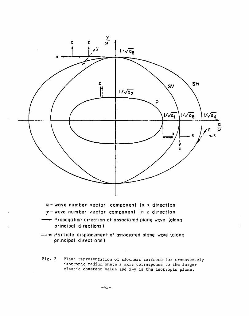
principal directions. .An itlustration of the slowness surfaces for

a transversely isotropic medium is shown in Fig. 2. Observe that

the values of the slownessess at the intersections of the surfaces

with the coordinate axes are the inverses of the phase velocities

presented in the previous section. The character of the corresponding

plane waves along the principal directions is also sketched, showing

the propagation and particle displacement directions.

-24-

GROUP VELOCITY

The group velocity Q (or velocity of energy propagation) for

the general anisotropic medium can be written according to Rayleigh's

energy argument [13] extended to three dimensional propagation as

[1]

'VG U =- -G,w (48)

where G is given by eqn. (18) and Q has the direction of 'VG or,

equivalently, the same direction as the normal to the slowness surface.

For points on the slowness surface G = 0, eqn. (48) can also

be written as

w'VG !!. = k.'VG (49)

where k is the wave number vector (a, a, y). Observe that the

correspondence between the wave number vector and the slowness vector

is [1,3]

k = ws (50)

such that k and s have the same orientation. The phase velocity in

the k direction can be represented vectorially by

wk (51)

-25-

If eqns. (49) and (51) are compared, it can be seen that

u • k - c • k (52)

Thus, the resultant of U in the c direction is £, which is

equivalent to saying that the velocity of energy propagation in

the direction normal to the wave front is equal to the phase

velocity.

Eqns. (48) through (52) are also valid for the two other

slowness surfaces. The same results are obtained if G is replaced

by H in the eqns. (48) through (52), provided that k is taken

accordingly. Thus, there are three phase velocities and three

group velocities for each direction in the medium.

Although eqn. (52) is satisfied, eqns. (49) and (51) indicate

that U and c are different. There is a component of energy velocity

in the direction parallel to the wave front, meaning that energy

transmission is not in the same direction as wave motion. This is

true for media where the phase speed varies with direction [1].

Thus, plane waves oblique to the principal directions can propagate

along their own normals only if energy is also supplied in a direction

parallel to the wave fronts.

-26-

APPLICATION EXAMPLE

Material Description

As an application example, a unidirectional composite material

was chosen. The material was 3M Scotchply type 1002 fiberglass epoxy

consisting of unidirectional E-glass in a 165 0 C curing epoxy

matrix. The composite prepreg tape was cured in a heated press at

6 2 0.69 10 N/m. The resulting resin content was 36 percent by

weight [18]. The properties of such composites depend not only on

the volume fraction of the components but also on the fabrication

method. Since knowledge of the elastic properties of the material

was necessary for the numerical calculations, samples were

fabricated for experiments. Ultrasonic methods [14,15,16,17] were

used for the experimental measurements, relating wave speeds and

elastic constants cij • The wave speeds were determined in the

through - transmission configuration using tone bursts to generate

either longitudinal or shear waves. The tests were performed at

frequencies from 0.5 to 2.25 MHz in increments of 0.25 MHz.

The test specimens were cut in the form of rectangular prisms

with uniform square cross sections from a 25.4 mm thick composite

plate. The cross-sectional area was square with 12.7 mm sides.

The lengths of the specimens ranged from 2.54 mm to 25.4 mm. The

test specimen axes were oriented at various angles with respect

to the fiber direction. The elastic constants were determined

-27-

from the measured longitudinal and shear wave speeds. The

experimental values for the elastic constants are given in Table 2.

The convention adopted for the transversely isotropic medium

in Fig. 1 was maintained here, so the z axis corresponded to the

fiber direction. 3 The density was 1850 kg/m according to the

manufacturer's data [18].

Slowness Surfaces

The slowness-surfaces for the fiberglass epoxy material were

calculated from G = 0 and H = 0, where G and H are given in eqns.

(18) and (20) respectively. The forms of these equations indicate

that both the surfaces are symmetric about y for a rectangular

coordinate system ~, S, and y. Thus, in order to determine the

surfaces, only their intecsections with the ~-y plane need to be

calculated. Then, the entire slowness surfaces can be generated

by revolving the intersection curves around the y axis. Additionally,

the intersection curves of the slowness surfaces G = 0 and H = 0

with the ~-y plane are symmetric with respect to ~ axis, which can

be checked by setting S = 0 in eqns. (18) and (20). By the

combination of all symmetries, only 1/4 of the intersections of

the surfaces on the ~-y plane need to be calculated. The positive

quadrant was chosen for the calculation.

The ranges of the variables are limited by the values shown

in Fig. 2 which can be obtained by setting S = 0 and alternately,

one at a time, ~ = 0 or y = 0 in eqns. (18) and (20). For the positive

quadrant the limits are:

-28-

For slowness surface SH: a < ~< 1/(a4)1/2 a :t.. 1/2

< ~ l/(aS) ; -w- w

For slowness surface SV: a a. 1/(as

)1/2 0 <:t.. < l(as)1/2; and < -< -w- -w

For slowness surface P: o < ~ < 11 (a ) 1/2 -w- 1 o ~ ~ ~ 1/(a

2)1/2.

The surfaces are generated by the successive combination of the

pairs (a.,y) satisfying eqn. (18) for SH and eqn. (20) for SV and P.

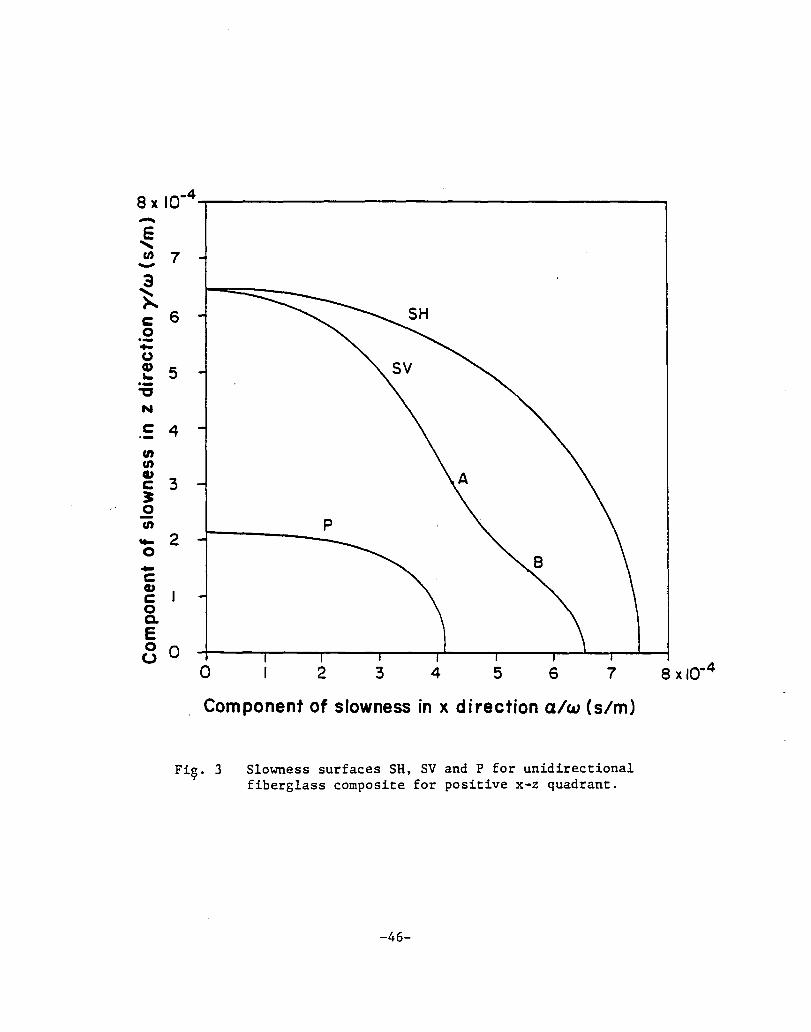
Fig. 3 shows the slowness surfaces SH, SV and P for the fiber-

glass epoxy composite. In Fig. 3, points A and B are the so-called

parabolic points on the slowness surface. At these points, the

gaussian curvature based on eqn. (23) is zero. Geometrically, these

are inflection points on the slowness surface. For the points of

zero gaussian curvature, the amplitude coefficient A (which corresponds n

to the inverse of a decay factor along the direction of the normal

to the surface) goes to infinity which would give infinite

displacement. The physical implications of the existence of such

points can be better understood by analyzing the wave surfaces.

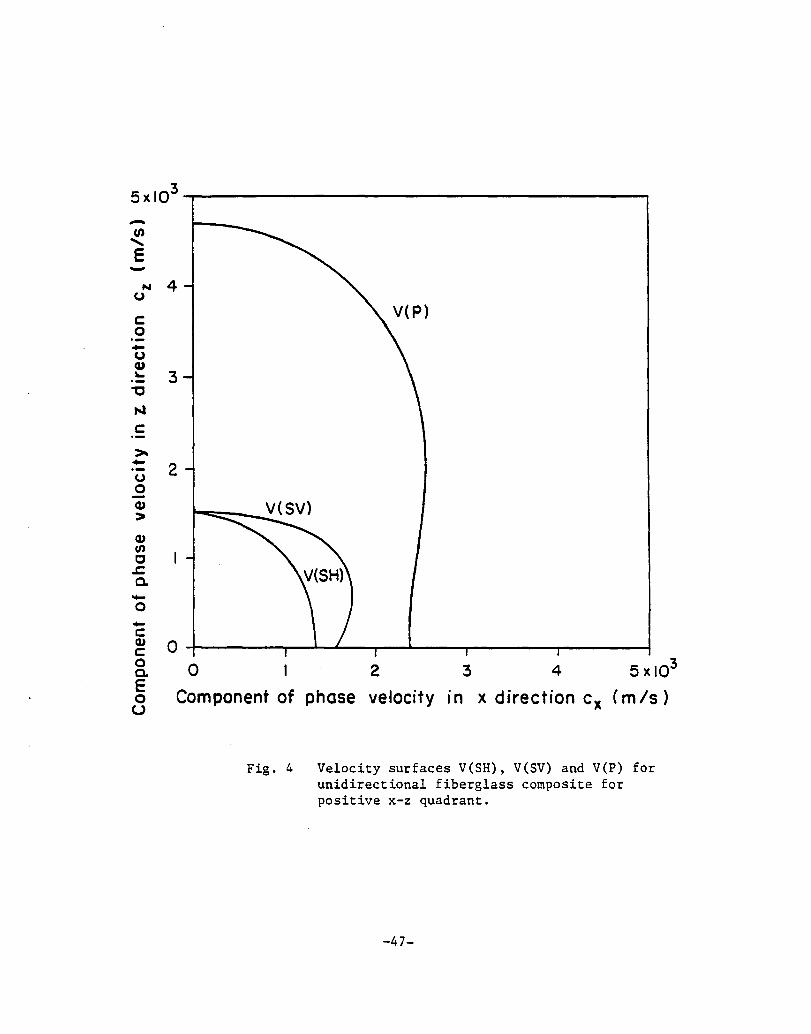
From the values obtained for slownesses, the velocity surfaces

were calculated using eqn. (44) and are shown in Fig. 4. The

velocity surfaces, namely V(SH) , V(SV) and V(P) correspond, respectively,

to the "inverses" of the slowness surfaces SH, SV and P.

Wave Surfaces

The wave surfaces can be directly obtained from the slowness

surfaces. It can be shown [1] that the coordinates x, y and z

of the wave surfaces can be calculated from -G, IG, ; -G, /G, ; a. w B w

and -G, /G, , respectively, for the wave surface corresponding to y w

-29-

the slowness surface SH, and by -H, /H, ;-H'a/H, ; and -H, /H, a w w y w

for the wave surfaces corresponding to the slowness surfaces SV

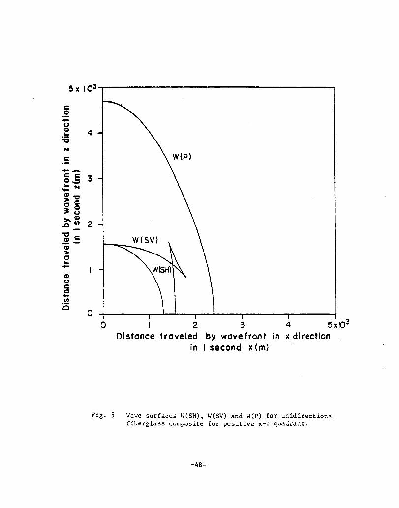
and P. Fig. 5 shows the wave surfaces as calculated from the

slowness surfaces SH, SV and P. The wave surface W (SH), which

corresponds to SH, has the smallest phase velocities. The wave

surface W(P), which corresponds to P, has the largest phase

velocities.

As shown in Fig. 5, the wave surface corresponding to SV has

two finite cuspidal edges [1,5]. The points at the tips of the

cuspida1 edges correspond to the inflection points A and B shown

in Fig. 3. The directions defined by the lines from the origin

to the tips of the cuspida1 edges (Fig. 5) represent the

directions for which the solution is not valid. These directions

can be found to be at 41.970 0 and 62.545 0 with r~spect to the z

axis. Since the wave fronts are geometrically similar in time,

the cuspidal edges will be always located in the same direction

with respect to the coordinate axes. Observe that for directions

between the angles defined above, radii from the origin to the

W(SV) wave surface may assume three distinct valu'es as can be seen

in Fig. 5, indicating that there are three contributions for the

displacements of points in this region of space. The contributions

arise because it is possible to find three points on the

corresponding slowness surface where the normals have the same

direction, according to the method of stationary phase. At a

-30-

point P in a direction in space between the angles 41.970° and 62.545,

three plane wave fronts can be seen traveling along the direction

OP from the origin (where the excitation is located). Thus, it is

possible to have plane wave fronts of different orientations and

different phase velocities passing through the same point in the

medium at different times. In reality these plane wave fronts

are segments that constitute the actual wave front.

-31-

Displacement Calculations

The displacements in a transversely isotropic medium subjected

to a point force excitation as shown in Fig. 1 were also calculated

for the fiberglass epoxy material.

A computer program was written that calculates the displacements

at a given point P(x,y,z) in the material. The following steps were

performed:

(1) Search for the point or points on each of the slowness

surfaces in which the outward normals are parallel to the direction

OP. This is done by comparing the direction defined by OP with the

direction of the gradients to the slowness surfaces. The program

retains the closest values to the direction given (one value for

slowness surface SH; up to three values for slowness surface SV and

up to two values for slowness surface P, in accordance with the

possible number of points having the same normal direction). The

wave numbers are determined from the coordinates of the selected

points on the slowness surfaces via eqns. (18) and (20).

(2) Check the signs of the gaussian curvature and the

direction of the gradient vector of the slowness surfaces, thus

establishing the resulting phase coefficient A • n

(3) Substitute into eqns. (36) through (38) the values found

for a, e and y and A above and calculate the contributions of each n

slowness surface to the displacements u, v and w.

-32-

Points in space were chosen and the corresponding displacements

calculated. For simplicity the points were placed on the coordinate

planes. The set of points chosen were:

(1) On the plane, points along the 2 + 2

:::0 4 2 and x-z arc x z m ,

(2) On the x-y plane, points along the 2 +

2 :::0 4 2 arc x y m.

The frequency was set at 1 MHz and a load (body force) of

unit amplitude (F = 1 N/kg) was applied. From eqns. (15), (16) and o

(17) it can be seen that if any of the gaussian curvatures is zero,

the correspond~ng displacement function assumes an infinite value.

It is known physically that no point in space may undergo an infinite

displacement since the amplitude of excitation F is finite. It can o

be shown [2] mathematically that the discontinuities can be eliminated

and the decay of the displacement amplitudes is found to vary as

-5/6 r In order to generate the amplitude coefficients, the points of

discontinuity on the slowness surface SV are "avoided", which is

equivalent to excluding the points A and B from the calculation set.

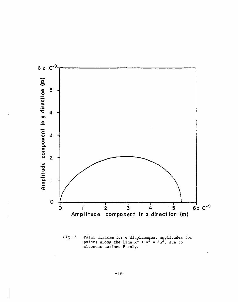
Figs. 6 through 9 show the polar diagrams of the displacement

amplitudes for the points 2 m away from the origin on the x-y plane.

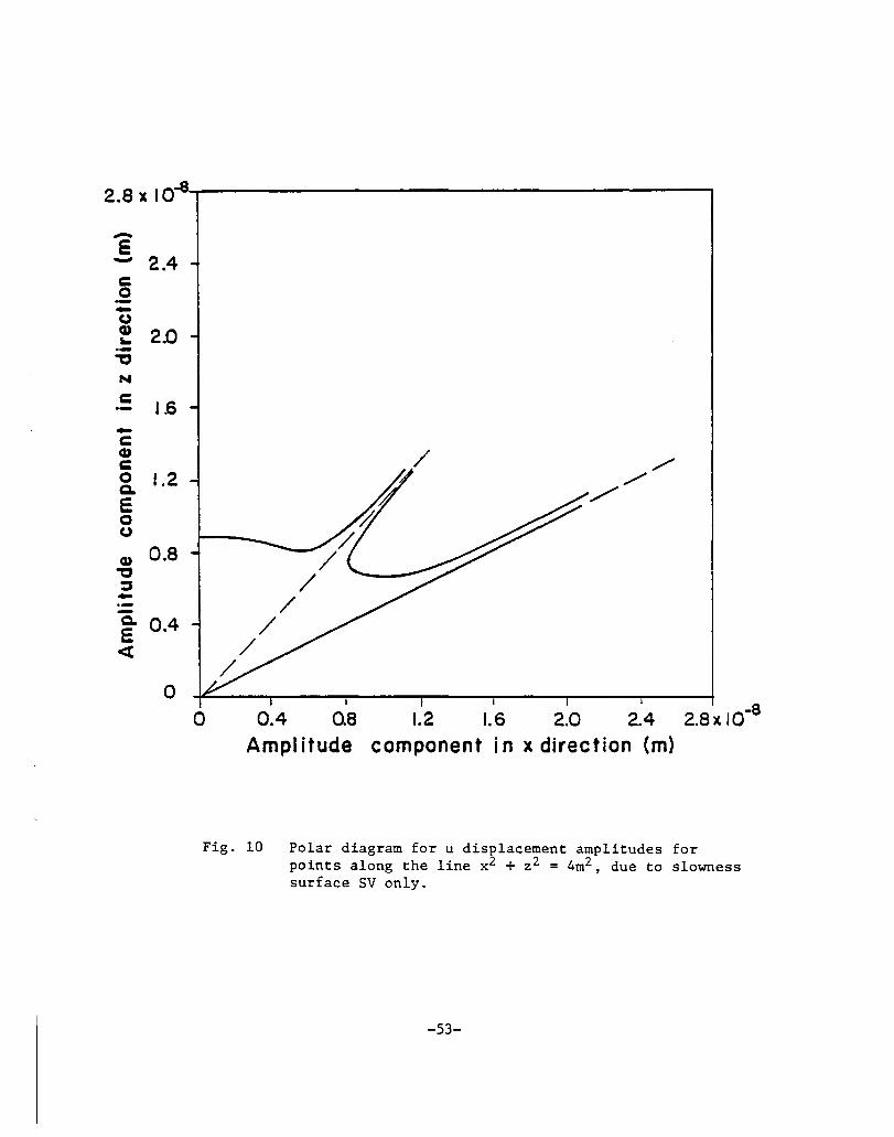
Figs. 10 through 13 show the polar diagrams of the displacements

amplitudes for the points 2 m away from the origin on the x-z plane.

Observe that by reasons of loading symmetry, v displacements for

points on the x-z plane are zero as well as w displacements for points

on x··y plane. The curves are plotted separately according to the

slowness surface that generates the contribution.

For points on the x-y plane, the contributions of the slowness

surface SV are zero which implies that there are no shear waves

-33-

propagating along x direction with particle displacement in the z

direction. Also, there are no shear waves propagating along the

y direction with particle displacement in the z direction.

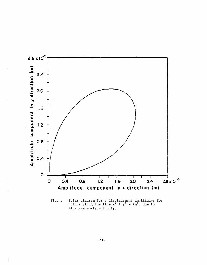
The contributions from the slowness surface P, Figs. 6 and

8, show that (1) there are pure longitudinal waves traveling along

the x direction and this is the direction of maximum amplitude for

u displacements (as expected since x is coincident with the force

line); (2) no longitudinal waves travel in the y direction (zero

amplitude component of v displacement for points in the y direction),

and no shear waves with y polarization travel in the x direction

(v displacements are zero in x direction).

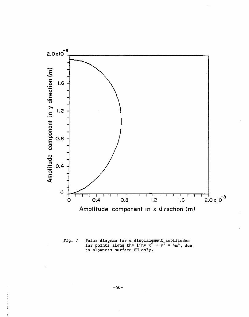
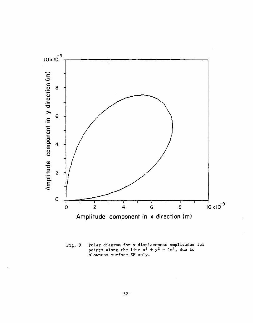
The contributions from the slowness surface SH, Figs. 7 and 9,

show that (1) there are pure shear waves in the y direction (with

x polarization direction) but since v displacements along the y

direction are zero, these are standing waves (y direction vibrates

as a string); (2) no longitudinal waves travel in the y direction

(zero amplitude component of v displacements for points in the

y direction), and no shear waves with y polarization travel in the x

direction (v displacements are zero in x direction).

For points on the x-z plane, the contributions of slowness

surface SH are zero which implies that there are no shear waves

propagating along the x direction with particle displacement in

the y direction. Also there are no waves propagating along the z

direction with particle motion in the y direction.

-34-

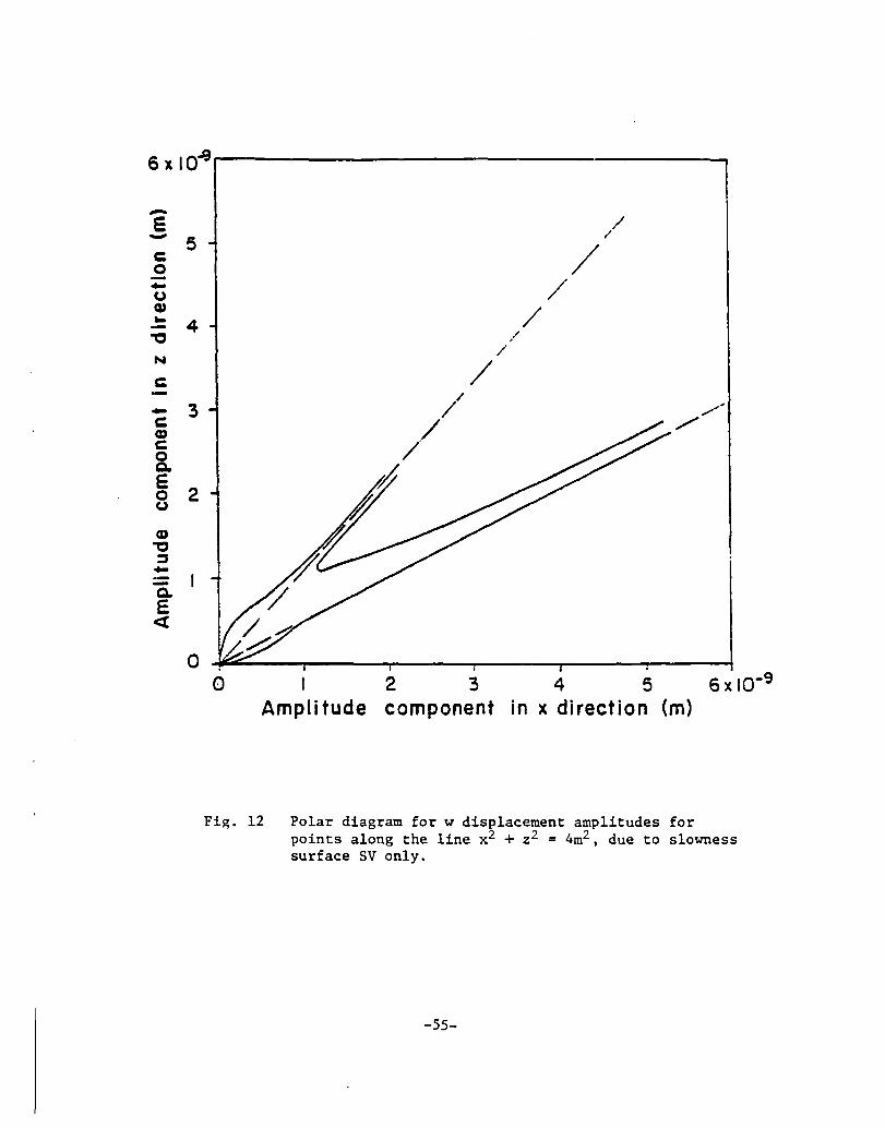
The contributions from the slowness surface SV, Figs. 10 and

11, show that (1) there are pure shear waves in the z direction (with

x polarization direction) but since the w displacements along the

z direction are zero these are standing waves (z direction vibrates as

a string); (2) there are no shear waves traveling along the

x direction (zero amplitude component of w displacement in the x

direction).

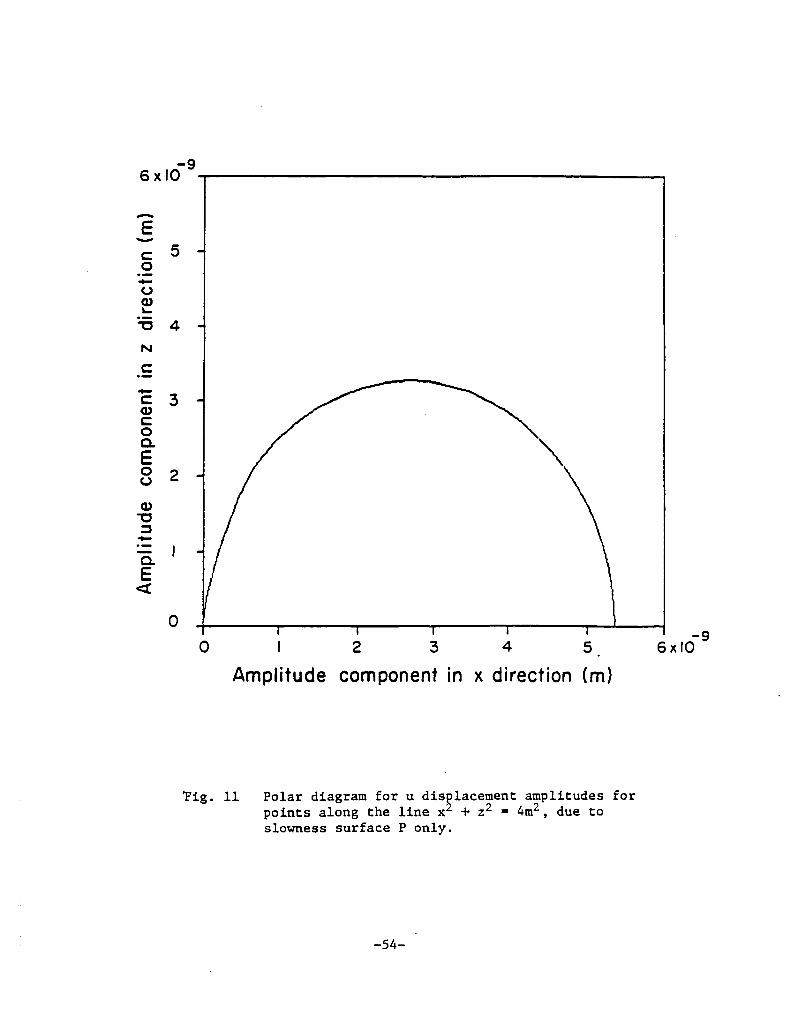
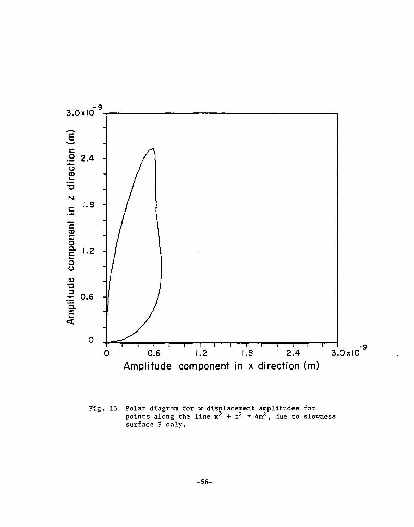
The contributions from the slowness surface P, Figs. 11 and 13,

show that (1) there are pure longitudinal waves propagating along

the x direction and the u displacement amplitude along the x direction

is larger than the corresponding u displacement amplitude along the

z direction; (2) there are pure shear waves in the z direction (with

x polarization direction) but since the w displacements along the

z direction are zero these are standing waves.

By observing the polar diagrams of displacements (Figs. (6)

through (13», it can be seen that there are characteristic directions

defining maxima for the displacement amplitudes. For comparison

purposes these directions are listed in Table 3. It can be observed

that there are two maxima for the contributions of slowness surface

SV corresponding to the inflection points A and B in Fig. 3. For

the contributions of the slowness surface P, the maxima occur at

two other distinct positions. For the points on the plane x-y,

the maxima occur along the line of force (x axis itself) for u

displacements except for the small contribution of SH (see Fig. 7),

-35-

and at 45° for v displacements as expected, since x-y is isotropic.

Slowness furfaces not I-is ted in Table 3 have zero contributions to

the corresponding displacements.

Recalling the relationship between strain energy and displacement

amplitude (energy is proportional to the square of amplitude), it

is clear that for points in regions of larger amplitudes the energy

will assume the higher values. The difference between anisotropic

and isotropic media is that the energy density for anisotropic media

is not a uniform function for equal solid angles having vertexes at

the origin, constructed around different directions in space.

Lighthill [2] referred to this phenomenon saying that the energy is

"confined" to some cone in space, or in other words, most of the

energy travels along preferential directions. The preferential

directions for the unidirectional fiberglass epoxy composite are

shown in Table 3. It is understood that the maxima are the center

directions of the regions around which the energy is confined. When

the numerical process is carried out the preferential directions are

automatically determined.

-36-

CONCLUSIONS

The far-field displacement pattern in an infinite transversely

isotropic medium subjected to an oscillatory point force was determined

and evaluated for a specific fiberglass epoxy composite. The solution

describes the stress wave field in terms of the geometric aspects

of the disturbance spreading by means of slowness and wave surfaces.

The solution for displacements allows the prediction of the amplitude

distribution as shown by the construction of polar diagrams.

"It was seen that the energy from a point source travels along

radial directions even if the wave surfaces assume complicated shapes,

meaning that the phase and group velocities are different.

The existence of preferential directions is an important aspect

to be considered when experimental tests are to be designed.

Knowledge of the displacement field allows a better choice to be

made for the positioning of components of the measuring system.

There appear to be no restrictions regarding the applicability

of this method to other types of anisotropy. If appropriate symmetry

relations can be applied as in the case of eqn. (7), the same

procedurescan be followed for the displacement field solution. This

possibility is attractive for use in the description of the stress

wave field of filamentary composite materials with fiber arrangements

other than unidirectional.

Another possible application is the study of acoustic emission

(AE) phenomena in composites or other anisotropic materials. It is

known that acoustic emission is a transient disturbance of relatively

small dimensions occurring inside the material, and normally

-37-

containing a range of frequency components. If the method is applied

for each component of frequency, superposition can be used for the

determination of the field resulting from the AE source. Knowledge

of the displacement field might allow inferences regarding the

source such as strength and orientation, and consequently perhaps

the degree of damage within the material.

-38-

REFERENCES

(1] M.J. Lighthill, "Studies on Magneto-Hydrodynamic Waves and other Anisotropic Wave Motions", Philosophical Transactions of the Royal Society, Series A, Vol. 252, 1960, pp. 397-430.

[2] V.T. Buchwald, "Elastic Waves in Anisotropic Media", Proceedings of the Royal Society, Series A, Vol. 253, 1959, pp. 563-580.

(3] J.L. Synge, "Elastic Waves in Anisotropic Media", Journal of Mathematics and Physics, Vol. 25, 1956, pp. 323-334.

(4] G.F. Carrier, "The Propagation of Waves in Orthotropic Media", Quarterly of Applied Mathematics, Vol. 4, 1946, pp. 160-165.

(5] M.J.P. Musgrave, Crystal Acoustics; Introduction to the Study of Elastic Waves and Vibrations in Crystals, Holden Day, San Francisco, 1970.

(6] J.D. Achenbach, A Theory of Elasticity with Microstructure for Directionally Reinforced Composites, OISM-Courses and Lectures, No. 167 (International Center for Mechanical Sciences), SpringerVerlag, N.Y., 1965.

(7] ,J .E. White and F .A. Angona, "Elastic Waves in Laminated Media", The Journal of the Acoustical Society of America,' Vol. 17, No.2, 1955, pp. 310-317.

(8] B.W. Rosen, "Stiffness of Fibre Composite Materials", Composites, Vol. 4, No.1, 1973, pp. 16-25.

(9] A.E.H. Love, A Treatice on the Mathematical Theory of Elasticity, Dover, 4th Edition, 1944.

(10] S.G. Lekhnistskii, Theory of Elasticity of an Anisotropic Elastic Body, Holden Day, San Francisco, 1963, (translation).

(11] I.S. Sokolnikoff, Mathematical Theory of Elasticity, McGraw Hill, NY, 1956.

[12] K.F. Graff, Wave Motion in Elastic Solids, Ohio State University Pre~s, 1975.

[13] L. Rayleigh, Theory of Sound, Vol. 2, Dover, 1945.

[14] G.D. Dean and F.J. Lockett, "Determination of the Mechanical Properties of Fiber Composites by Ultrasonic Techniques", Analysis of the Test Methods for High Modulus Fibers and Composites, ASTM STP52l, American Society for Testing Materials, 1973, pp. 326-345.

-39-

[151 G.D. Dean, "Characterization of Fibre Composites using Ultrasonics", Composites-Standards, Testing and Design, National Physics Laboratory Conference Proceedings, Middlesex, England, 1974, pp. 126-130.

[161 J.H. Williams, Jr., H.N. Hashemi and S.S. Lee, "Ultrasonic Attenuation and Velocity in AS/3501-6 Graphite/Epoxy Fiber Composite", Journal of Nondestructive Evaluation, Vol. 1, No.2, 1980, pp. 137-148.

[171 M.F. Markham, "Measure~ents of the Elastic Constants of Fibre Composites by Ultrasonics", Composites, Vol. 1, No.3, 1970, pp. 145-149.

[181 !'Scotchply Reinforced Plastics Technical Data - Type 1002", 3M Company, Minnesota, May 1, 1969.

-40-

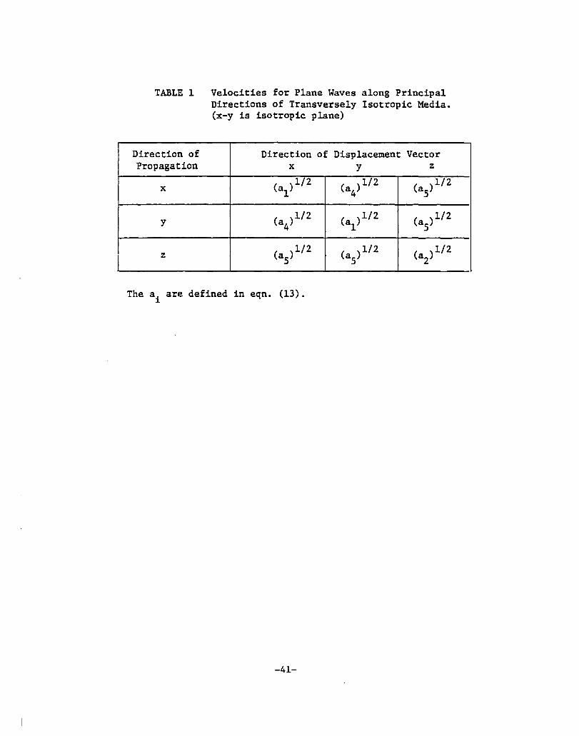
TABLE 1 Velocities for Plane Waves along Principal Directions of Transversely Isotropic Media. (x-y is isotropic plane)

Direction of Direction of Propagation x

x (a1)1/2

y (a4

)1/2

z (a5

)1/2

The a. are defined in eqn. (13). ~

-41-

Displacement Vector y z

(a4)1/2 (a

5)1/2

(a1

)1/2 (a5)1/2

(a5

)1/2 (a2)1/2

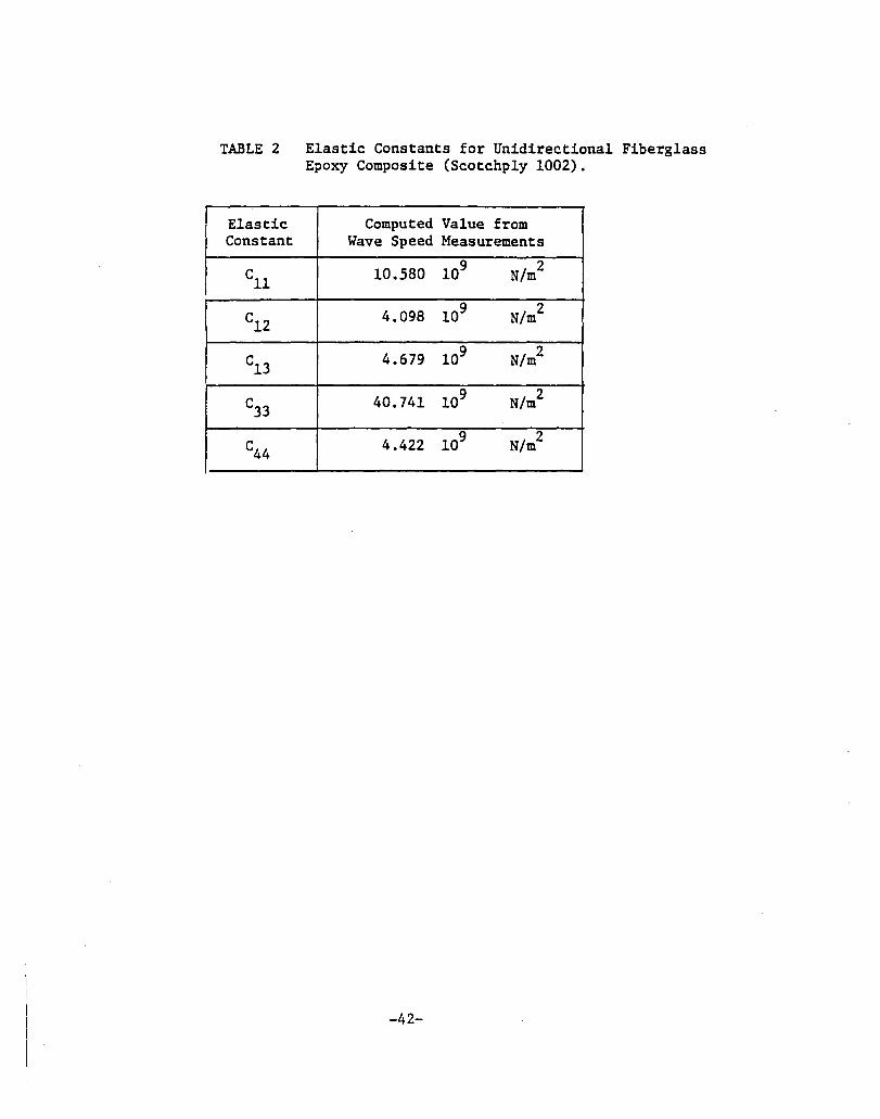
TABLE 2 Elastic Constants for Unidirectional Fiberglass Epoxy Composite (Scotchply 1002).

Elastic Computed Value from Constant Wave Speed Measurements

Cll 10.580 109 N/m2

C12 4.098 109

N/m 2

C13 4.679 109 N/m2

C33 40.741 109 N/m2

C44 4.422 109 N/m2

-42-

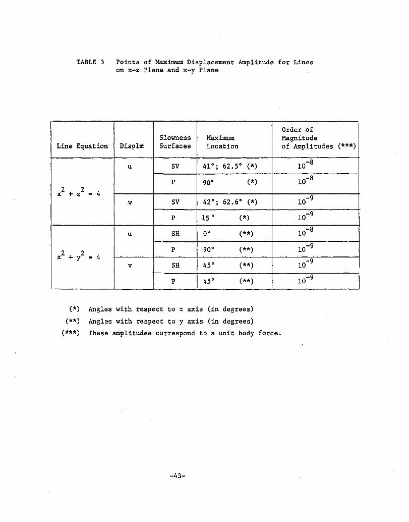
TABLE 3 Points of Maximum Displacement Amplitude for Lines on x-z Plane and x-y Plane

Slowness Maximum Line Equation Displm Surfaces Location

u sv 41 0; 62.5° (*)

P 90° (*) 2

+ z 2

4 x = W. SV 42°; 62.6° (*)

P .15 ° (*)

u sa 0° (**)

x2 + y2 P 90° (**)

= 4 v SH 45° (**)

t--

P 45° (**)

(*) Angles with respect to z axis (in degrees)

(**) Angles with respect to y axis (in degrees)

(***) These amplitudes correspond to a unit body force.

-43-

Order of Magnitude of Amplitudes

10-8

10-8

10-9

10-9

10-8

10-9

10-9

10-9

(***)

I

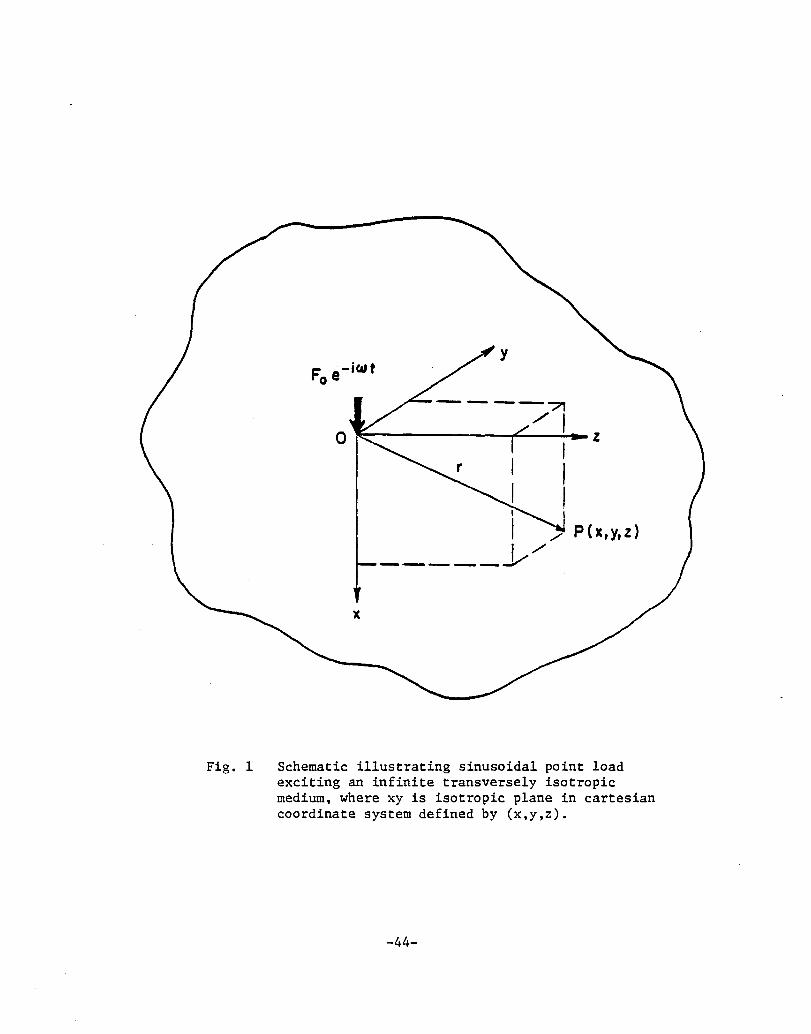
Fig. 1

----~

/1 o~------~:...----::..-z

I

x

I I I

I /' 1/

------~

I , p (X,Y. z)

Schematic illustrating sinusoidal point load exciting an infinite transversely isotropic medium, where xy is isotropic plane in cartesian coordinate system defined by (x,y,z).

-44-

z z L w

z

t 11./02

a- wave number vector component in x direction y-wave number vector component in z direction

- Propagation direction of associated plane wave (along principal directions)

--- Particle displacement of associated plane wOIe (along · principal d irecti ons)

Fig. 2 Plane representation of slowness surfaces for transversely isotropic medium where z axis corresponds to the larger elastic constant value and x-y is the isotropic plane.

-45-

1/-1ci4

a

8 x 10-4

-e " en 7 -:3 ~ c 6 0 .-+-CJ Q) 5 .. . -~

N

c: 4 fit fit .,

3 c :s 0 fit .. 2 0 +-c: G)

c 0 0. E 0 0 (,)

0 2 3 4 5 6 7

Component of slowness in x direction a/w (s/m)

Slowness surfaces SR, SV and P for unidirectional fiberglass composite for positive x-z quadrant.

-46-

8 x 10-4

5xI03,-----------------------------------------~

-en ....... E -

N 4 (J

c o

-

-o -c: w c: o Co E o u

2

o ~--------~~~--_r--~----~------~--------~ o 2 3 4 5 x 103

Component of phase velocity in x direction Cx em/s)

Fig. 4 Velocity surfaces V(SH), V(SV) and V(P) for unidirectional fiberglass composite for positive x-z quadrant.

-47-

5x 103-------------------------------------------

c o -CJ ~ 4 :a N

c:

--c e 3 0_ ~ N ~

CD-a :> c: c 0 3 u ~Q,) ~ f/J 2

-c:Jc: ~-CD :> o ~ -CD (J

c c -(J) .-o o

o 2 3 4

Distance traveled by wavefront in x directton in I second x (m)

Fig. 5 I,ave surfaces t~(SH), W(SV} and W(P) for unidirectional fiberglass composite for positive x-z quadrant.

-48-

6 x 10-9

-e -c 5 0 -u OJ ... . -~ 4 >-c -c

3 OJ c 0 ~

e 0 u 2 OJ ~ ~ --~ e «

o o 1 2 3 4 5

Ampl itude component in x direct ion (m)

Fig. 6 Polar diagram for u displacement amplitudes for points along the line x2 + y2 = 4m2 , due to slowness surface P only.

-49-

-8 2.0x10

-E -c: 0 -(,J Q,) ~

"C

~

c:

-c: Q,)

c: o

1.6

1.2

E 0.8' o (,J

Q,)

"C ::l - 0.4 a. E «

o

Fig. 7

0.4 0.8 1.2 1.6

Amplitude component in x direction (m)

Polar diagram for u displac~ment arnpli~udes for points along the line x + y2 = 4m , due to slowness surface SH only.

-50-

-8 2.0 It 10

2.8xIO~~--------------------------------------~

-e -c: o -u

2.4

~ 2.0 "0 :>.

c:

1.2 1.6 2.0 2.4


Fig. 8 Polar diagram for v displacement amplitudes for points along the line x2 + y2 = 4m2 , due to slowness surface P only.

-51-

-9 IOxlO ~--------------------------------------~

-E -g 8 -u Q) ~

"0

~

c:

-c: Q) c: 0 c. E 0 u

Q)

"0 ::J -a. E <r

6

4

2

0

o 246 8


Fig. 9 Polar diagram for v displacement amplitudes for points along the line x2 + y2 = 4m2 , due to slowness surface SH only.

-52-

2.8xIO~;------------------------------------------'

-e - 2.4 c o --Co)

~ 2.0 ~

N

C

-c CD c

1.6

&. 1.2 e o Co)

CD 0.8 ~ ~ -~ 0.4 <t

o

/

o 0.4 0.8 1.2 1.6 2.0 2.4 Ampl itude component in x direction (m)

-8 2.8x10

Fig. 10 Polar diagram for u displacement amplitudes for points along the line x2 + z2 = 4m2 , due to slowness surface SV only.

-53-

6xIO-9~--------------------______________________ ~

-E -c: 0 -0 Q) '-~

N

c:

-c: Q) c: 0 ~

E 0 0

Q)

~ ~ -c. E

<l:

5

4

3

2

o o 2 3 4 5


'Fig. 11 Polar diagram for u displacement amplitudes for points along the line x2 + z2 = 4m2 , due to slowness surface P only.

-54-

-9 6xlO

6 x 10-9

-e - 5 C 0 -u Q) ~ 4

" N

c

- 3 C Q) c 0 a-E

2 0 u

Q)

" :J -.--a-S ex

0

/ /

/ /'

/ , ,. /

/ .,,/

/'"

0 I 2 3 4 5 6 x 10-9


Fig. 12 Polar diagram for w displacement amplitudes for points along the line x2 + z2 = 4m2 , due to slowness surface SV only.

-55-

-9 3.0x10

-E -c: 0 -(,J Q) ~

~

N

c::: -c::: Q) c:: 0 Co

E 0 u Q)

~ ::l -Co

E <X:

2.4

1.8

1.2

0.6

0 -9

0 0.6 I. 2 1.8 2.4 3.0 x 10


Fig. 13 Polar diagram for w displacement amplitudes for points along the line x2 + z2 = 4m2 , due to slowness surface P only.

-56-

1. Report No. 2. Government Accession No.

NASA CR-4001 4. Title and Subtitle

Wave Propagation in Anisotropic Medium Due to an Oscillatory Point Source With Application to Unidirectional Composites

7. Author(s)


9. Performing Organization Name and Address

Massachusetts Institute of Technology Department of Mechanical Engineering Cambridge, Massachusetts 02139

12. Sponsoring Agency Name and Address

National Aeronautics and Space Administration Washington, D.C. 20546

15. Supplementary Notes

3. Recipient's Catalog No.

5. Report Date

July 1986 6. Performing Organization Code

8. Performing Organization Report No.

None

10. Work Unit No.

11. Contract or Grant No.

NAG3-328 13. Type of Report and Period Covered

Contractor Report

14. Sponsoring Agency Code

506-43-11 (E-3093)

Final report. Project Manager, Alex Vary, Structures Division, NASA Lewis Research Center, Cleveland, Ohio 44135.

16. Abstract

The far-field displacements in an infinite transversely isotropic elastic medium subjected to an oscillatory concentrated force are derived. The concepts of velocity surface, slowness surface and wave surface are used to describe the geometry of the wave propagation process. It is shown that the decay of the wave amplitudes depends not only on the distance from the source (as in isotropic media) but also depends on the direction of the point of interest from the source. As an example, the displacement field is computed for a laboratoryfabricated unidirectional fiberglass epoxy composite. The solution for the displacements is expressed as an amplitude distribution and is presented in polar diagrams. This analysis has potential usefulness in the acoustic emission (AE) and ultrasonic nondestructive evaluation of composite materials. For example, the transient localized disturbances which are generally associated with AE sources can be modeled via this analysis. In which case, knowledge of the displacement field which arrives at a receiving transducer allows inferences regarding the strength and orientation of the source, and consequently perhaps the degree of damage within the composite.

17. Key Words (Suggested by Author(s))

Elastic waves; Ultrasonics; Acoustic emission; Wave propagation analysis; Nondestructive testing; Fiber reinforced composites

18. Distribution Statement

Unclassified - unlimited STAR Category 38

19. Security Class if. (of this report)

Unclassified 20. Security Classlf. (of this page)

Unclassified 21. No. of pages

58

"For sale by the National Technical Information Service, Springfield, Virginia 22161

22. Price·

A04

NASA-Langley, 1986

End of Document

Documents

Wave Propagation in Anisotropic Medium Due to an