Embed Size (px)
Citation preview
WAGE INEQUALITY AND CRIMINAL ACTIVITY:AN EXTREME BOUNDS ANALYSIS FOR THE UNITED STATES -- 1975-1990
RICHARD FOWLES University of Utah
MARY MERVA University of Utah
The past decade in the United States has been characterized by a widening in thedistribution of wage income. While much research has attempted to uncover the causes ofthese earnings trends, much less is known about their impact upon social and economicfactors. This study examines evidence for links between changes in distribution of wageincome and criminal activity. Using extreme bounds analysis in conjunction withordinary least squares regression, this paper shows that robust results linking wageinequality and crime are obtainable across a rich set of model specifications for theviolent crimes of murder and assault. No evidence is found linking wage inequality withthe crimes of robbery and burglary. Results are inconclusive for larceny/theft, motorvehicle theft, and forcible rape. These results should be viewed as a first stage inexamining the link between wage inequality and criminal activity. Research into thespecific behavioral complexities underlying these relationships needs to be considered toaffirm these results.
*The authors benefited from the insightful comments of Jared Bernstein, Irv Garfinkel, RobertHaveman, Harold Watts, the editior and three anonymous referees. Financial support came fromthe Economic Policy Institute on topics related to this research. Additional thanks to SolomonNamala and Bassam Abual Foul for research assistance.

1
WAGE INEQUALITY AND CRIMINAL ACTIVITY:AN EXTREME BOUNDS ANALYSIS FOR THE UNITED STATES -- 1975-1990
INTRODUCTION
A striking feature of the United States economy to emerge during the past decade has
been a widening in the distribution of wage income (Mishel and Bernstein, 1993). For example,
over the 1979 to 1988 period, the ratio of the college educated workers’ wage relative to the high
school educated workers’ wage increased by over 15 percentage points (Bound and Johnson,
1992). While much research has attempted to uncover the causes of these earnings trends (Blank
and Card, 1993; Bound and Johnson, 1992; Murphy and Welch, 1991; Bluestone and Harrison,
1988), much less is known about their impact upon social and economic factors.1 This study
examines evidence regarding the links between the deterioration in the distribution of wage
income and social pathologies, namely criminal activity. Ascertaining the relationship between
wage inequality and criminal activity has important theoretical and policy implications.
From a theoretical perspective, the relationship between inequality and crime is generally
thought to operate via an individual’s assessment of the equity of a particular distribution of
economic resources. This assessment is, in part, determined by the socio-cultural environment of
the individual. Given that an individual perceives the distribution of income to be inequitable,
two possible interdependent responses could result in higher rates of criminal activity. First,
some individuals may resort to property crime as a method to address their grievances. Second,
the perceived unfairness may generate feelings of frustration and anger, which in extreme cases
can manifest themselves in the form of violent criminal behavior. This theory would then
suggest that economic inequality is positively correlated with both property and violent crimes.
The relationship between wage inequality and criminal activity is also an interesting topic
because of its policy implications. If this relationship exists and is of a reasonably strong
magnitude, then it raises the issues of income redistribution programs or programs that equalize
1 These earnings trends can be traced primarily to several interdependent developments,
namely, factors affecting the demand for low skill labor such as foreign competition, decliningunionization, and technological change; growth of service sector employment; and relativechanges in the supply of labor.
2
economic opportunities as tools to reduce criminal activity.
THEORETICAL BACKGROUND: INEQUALITY AND CRIME
The causal factors relating inequality and criminal activity has been the subject of much
research that covers a wide theoretical spectrum. Messner and Tardiff (1986) have classified
these as including: neoclassical economic theory (e.g., Becker, 1968; Ehrlich, 1973), Marxist
theory (e.g., Gordon; 1971), anomie theory (e.g., Merton, 1938, 1957), and macrostructural
sociological theory (e.g., Blau and Blau, 1982). The common denominator of this research is the
unambiguous positive relationship postulated between economic inequality and crime. An
important causal mechanism underlying this relationship is relative deprivation -- how an
individual (or group) perceives, as fair or unfair, the inequities in the distribution of income.
Relative deprivation is based upon the pervasive need for comparison between
individuals or groups within a society. Comparison of one’s position relative to that of others (or
one’s past) is a way of assessing how satisfied one is (e.g., Diener, 1984; Morawetz et al., 1977;
Easterlin, 1974; Dusenberry, 1952; Merton, 1938; Veblen, 1934). For example, Easterlin’s study
(1974) examines the empirical relationship between reported happiness and income and
concludes that individual happiness is not determined by absolute income levels, but by income
relative to a what they think they ought to have. This type of behavior highlights the relationship
between relative deprivation and subjective-well-being which is best summarized by Karl Marx:
"A house may be large or small; as long as the surrounding houses are equallysmall it satisfies all social demands for a dwelling. But if a palace rises beside thelittle house, the little house shrinks into a hut." (Marx, 1933:268--269).
Whether or not individuals assess a given distribution of income as inequitable is a
function of their socio-cultural environment. Relative deprivation may not be a significant
characteristic in societies which view economic inequality as an acceptable outcome based on
cultural and religious values (Stack, 1984). Two structural factors necessary for inequality to
give rise to relative deprivation are: (I) how the culture defines the “ends,” which are used to
measure success of individuals in society; and (ii) the economic opportunities (legitimate or not)
3
which provide the “means” for obtaining the proscribed “ends.” In 1938, the sociologist Robert
K. Merton wrote:
"It is only when a system of cultural values extols, virtually above all else, certaincommon symbols of success for the population at large while its social structurerigorously restricts or completely eliminates access to approved modes ofacquiring these symbols for a considerable part of the same population, thatantisocial behavior ensues on a considerable scale." (Merton, 1938:680).
At issue today is not simply Merton's restrictive social structure, but rather the restrictive
economic structure experienced by the majority of U.S. workers since the late 1970's. During
this time period, both the absolute and relative monetary rewards for legitimate economic
activities among lower skilled workers deteriorated. This has occurred in conjunction with a
stress on material gains over this same period of time. Thus, the economic and social structure of
the past decade may impose the sufficient conditions that link economic inequality with relative
deprivation. Next, consideration must be given as to why individuals would pursue criminal
activities in response to feelings of deprivation.
Not all individuals who perceive the distribution of economic resources as unfair resort to
criminal activities. Other avenues exist for addressing these grievances such as taking part in
legitimate economic opportunities (for example, augmenting human capital) or political activities
(for example, voting on tax proposals). Individuals may also direct feelings of anger and
frustration towards themselves. In extreme cases, these latent feelings may manifest themselves
as violent criminal activities. Other individuals may resort to property crimes, violent or not, as
methods to redistribute economic resources and satisfy their sense of injustice. In sum, as argued
by Merton (1957:27), "those who find themselves denied the positions which the egalitarian
myth has led them to believe are open to them may be driven to adopt high but 'deviant'
ambitions."
EMPIRICAL REVIEW AND STATISTICAL METHODOLOGY
While a direct relationship between crime and income inequality is supported by theory,
the exact specification of this relationship is not known. The empirical research on the
relationship between income inequality and criminal activity in the United States has so far
4
yielded conflicting results (see e.g., Messner and Tardiff, 1986; Williams, 1984; Bailey, 1984;
Blau and Blau, 1982; Messner, 1982; Jacobs, 1981; Danziger and Wheeler, 1975). These
empirical results are summarized in Table 1. This list is not exhaustive but does illustrate the
variety of results obtained.
These mixed results may arise because each of these studies presents a particular model
opening them to the critique that their results may be fragile and an artifact of model
specification (selective reporting). For example, Blau and Blau (1982) found a positive
relationship between inequality and murder while Messner (1982) found no significant
relationship. This statistical ambiguity (specification error) is characteristic of empirical
research when theory is vague about the exact relationship between variables and a true model
cannot be articulated; it is illustrative of Leamer’s "con" in econometrics (Leamer, 1983). The
stability and interpretability of the estimated regression coefficients is compounded when there
exists a high degree of collinearity amongst the explanatory variables relative to their degree of
correlation with the dependent variable. This is what Land et al. (1990) term the “partitioning
fallacy.” Even if there is low zero-order correlation amongst the explanatory variables, low
correlation between the explanatory variables and the dependent variable may lead to problems
with stability and interpretability of the estimated regression coefficients.
Since the goal of this analysis is to detect if there exists a consistent relationship between
inequality and crime we examine a range of plausible model specifications using an econometric
technique that specifically allows for the consideration of a wide array of models. As such, our
results should be viewed as exploratory and descriptive instead of estimative in nature. This
econometric technique is known as extreme bounds analysis (EBA) (see Leamer, 1983).
EBA addresses the issue of specification uncertainty by computing the maximum and
minimum coefficients that could be obtained using maximum likelihood estimation on a large set
of model specifications. The highest and lowest estimates are called the upper and lower bounds.
If these bounds cover zero (known as fragile or loose bounds), then either negative or positive
coefficients could be obtained from the data depending on the model specified. If the upper and
lower bounds do not cover zero (known as non-fragile or tight bounds), then all possible
specifications would yield an unambiguous sign on the coefficient of interest. Standard ordinary

5
least squares (OLS) estimates are contained within these bounds. Thus EBA provides additional
information on relationships within the data regarding specification uncertainty that may not be
apparent in conventional reporting styles which emphasize sampling uncertainty and assume the
true model in known.
Conventional reporting often presents t-statistics or p-values for the best fitting results or
for those that may conform to a researcher’s prior beliefs. Usually the best fit is uncovered after
a model search. In a model specification search, variables are typically dropped or introduced
until search criteria are satisfied. The selective reporting of conventional statistics based on this
sort of search may be misleading since the sampling properties of the estimators are not known
(see Hill, 1985). Further, statistically significant findings based on specification searches may be
associated with loose bounds and therefore not robust with respect to another model
specification. For a stimulating discussion on the abuses of reporting styles in econometrics see
Leamer (1983).
To avoid issues of selective reporting based on model specification uncertainty, we feel
that reporting EBA and standard output together can provide a clearer picture of the statistical
relationships within the data by examining how robust the empirical links are between inequality
and criminal activity. The range of possible estimates computed under EBA provides policy
makers with better information and certainty regarding possible outcomes that may not be
apparent when only a single set of point estimates are used. EBA highlights the fact that
contradictory statistical conclusions are possible and clarifies some of the sources of the
ambiguity.
The operational methodology of EBA partitions the set of explanatory variables into two
subsets: focus and doubtful. The focus set is comprised of variables that are always considered
in a model. The doubtful set is comprised of variables that may or may not be included in every
regression.2 Because of multicollinearity between the explanatory variables, different specif-
2 From a Bayesian perspective, minimal priors exist on the coefficients of the doubtful
set, in particular, the prior mean is centered at zero with a positive definite symmetric variance-covariance matrix. This is more fully discussed in a statistical appendix that is available from theauthors.

6
ications (choice of variables from the doubtful set) result in different regression estimates on the
coefficients of variables from the focus set. An estimate is fragile if the possible range of an
estimate on a focus variable derived over a wide variety of specifications from the doubtful set
covers zero. EBA can be viewed as an extension to all-subsets regressions where the data are
partitioned into the focus and doubtful set. If there are k doubtful variables then there are 2k
possible regression specifications when a variable is either included or excluded. A researcher
examining the effect of capital punishment (a focus variable) on murder rates might “search”
over sets of regressions that include other variables to discover a specification that supports his
or her beliefs. EBA goes beyond subsets regressions by examining all possible linear
combinations of the doubtful variables. The flavor of the analysis is Bayesian in spirit to the
extent that excluding a particular variable from a regression is equivalent to a prior belief that the
effect of that variable is zero with probability one. Instead of excluding variables, EBA allows
their effects on estimates of the coefficients of focus variables to be exposed in a vigorous way.
Partitioning variables into focus and doubtful sets reflects the issue under study. In this paper, in
addition to a constant term, our focus set includes only economic stress variables. Other
variables are undoubtably important, but by narrowing the focus set we can more strongly expose
inferential fragility.
The data used in this study are an aggregative pooled time-series, cross-sectional set
where metropolitan statistical areas (MSAs) are the unit of analysis over the period 1975 to 1990
in the United States. We use aggregative data instead of microdata to amplify any consistent
relationships between income inequality and crime. At the micro level the probability of
detection may be too slight because any effect would be diffused by more pronounced correlates.
Our choice of MSA as the unit of analysis is to retain heterogeneity at a community level. The
choice of MSA as a unit of analysis for this type of study is subject to debate. Messner and
Tardiff (1986) and Bailey (1984) argue that smaller geographic units such as neighborhoods or
cities are more appropriate statistical units of analysis rather than more geographically dispersed
MSAs. They reason that relative deprivation is only operational when individuals can actually
perceive differences in income distribution which can only occur in small, close geographical
units. However, information regarding the economic status of others may also be transmitted by

7
the media so it is not clear that the geographical unit need be spatially small. We use MSAs
because for the time period we are examining (1975 to 1990) the sample size in the Current
Population Survey is insufficient for computation of key variables for many smaller geographical
units. This problem is not present for studies using decennial census data. We also believe that
MSAs give us the advantage of increased variability in the data which may not be present with
smaller geographical units such as neighborhoods as utilized by Messner and Tardiff (1986).
Messner and Tardiffs’ study concludes that income inequality has no effect on homicides,
however it is likely that the variability of income inequality in their data is not adequate to detect
any relationship. (The coefficient of variation on the Gini coefficient in their data is
approximately half of what it is in other studies using MSAs.)
Using a pooled time-series, cross-sectional data to estimate models can be statistically
cumbersome. Therefore, the most basic model form is used in this study. Technically, we are not
as concerned with providing the most efficient estimators as we are with discovering the signs of
the relationships. Additionally, since the correct model specification is not known, simpler
models are less vulnerable to the problem of overconfidence in estimation (Sayrs, 1989). Our
models take the simple form:
Yi,t = β0 + ΣjβjXj,i,t + ΣkΓkzk,i,t + εi,t
where
β's are unknown economic stressor parameters;
Γ's are unknown control parameters; and
ε is an unknown disturbance.
Yit represents a stress outcome measure for the ith MSA for the tth time period, Xj,i,t represents the
j th focus variable, and Zk,i,t the kth doubtful variable. In particular, the outcome, or dependent
variables include categories relating to violent crimes and property crimes.
The stress outcome variable for the ith MSA is the reported crime rate per 100,000
population from the Uniform Crime Reports for the crime categories of aggravated assault,
murder/nonnegligent manslaughter, motor vehicle theft, larceny/theft, robbery, burglary, and
forcible rape. The focus variables, which are included in any specification, are those considered

8
to be the minimum controls necessary to specify a credible economic stress model. These
variables include a constant term, an unemployment effect, the poverty rate, and a wage
inequality coefficient. (Since the affect of wage inequality on crime is the focus of this paper a
discussion of this variable follows). The set of doubtful variables includes a time trend variable,
percent of the population that is non-white, percent of population ages 16 to 21, population
density, percent of workers with at least some college education, and a southern regional dummy
variable. Dummy variables for each MSA are not included in the model because of degrees of
freedom problems that arise when using cross-sectional data set that exhibits greater width (28
observations per year) than depth (15 years) (see Greene, 1993:479).
We use wage inequality instead of income inequality for several reasons. First, increasing
wage inequality has shown a significant trend over the time period of 1973 to 1993. Over this
period, wage inequality has increased both within groups of workers with similar educational and
experience levels, and between groups of workers by educational and experience levels (see
Mishel and Bernstein, 1994:136-138). Second, wage inequality is likely to be a cleaner measure
of economic inequality given the systematic misreporting of income that makes income
inequality measures by MSA’s unreliable. Finally, wage inequality has a lower correlation with
poverty because not all income components used to compute poverty levels are included in wage
inequality measures. Changes in wage inequality, however, are presumably tied to changes in
income inequality (Blank and Card, 1993) and so one could view wage inequality as a good
proxy or instrumental variable for income inequality.
Our measures of wage inequality are computed over a sample of all workers from the
Bureau of Census’s Current Population Survey (CPS) who report usually working 30 hours or
more per week. This group of workers has a significant commitment to the labor force and
therefore we are not capturing the rise in temporary and part-time employment that has occurred
over the years from 1975 to 1990. As such, our measure of wage inequality is a conservative
estimate of the widening in the distribution of wage income. To insure adequate sample size in
the computation of this variable we are restricted by the availability of data to MSA’s which have
relatively large populations and thus adequate CPS sample size. This constrains us to examine
28 major MSAs and our results should be viewed in this context.
9
The paper considers six standard measures of wage inequality because, while there may
be agreements regarding what constitutes an unequal distribution of income, there is no
theoretical consensus regarding what weights to apply to the tails of the distribution. The breadth
of these measures allow us to consider inequality as a result of extremely high or low wages, or
inequality due to moderate wage disparity. Four measures of wage inequality are based on the
Lorenz area and include the Gini, Mehran, Piesch, and Bonferroni coefficients. These measures
of income inequality can be defined in terms of a Lorenz diagram as: I = ∫V(p)[Lr(p) - L(p)]dp
(Nygard and Sandstrom, 1981) where p is the percentile of the distribution, L(p) is the actual
distribution, Lr(p) is a reference distribution, and V(p) is a weight function on the discrepancy
between the reference and the actual distribution. If the reference distribution is the egalitarian
distribution, Lr(p) = p then the integral measure a weighted area between the actual distribution
and a diagonal line in a Lorenz diagram. V(p) allows for measures of this area to emphasize
discrepancies in lower or higher incomes. For the Gini, Mehran, Bonferroni, and Piesch this
function is 2, 6(1-p), 1/p, and 3p, respectively. The Gini coefficient weights extreme incomes,
the Piesch high incomes, and the Mehran and Bonferroni low incomes. For a detailed discussion
on the properties of these and other indexes, see Nygard and Sandstrom (1981) and
Champernowne (1974). For discussion on the relationship between the Gini coefficient and
relative deprivation see Yitzhaki (1979) and Hey and Lambert (1980). In addition to these Lorenz
measures, the coefficient of variation in wage income and the coefficient of interquartile
variation of wage income are also analyzed.
Finally, during the period of the study, examination of the data show rich cyclical
variability which lessens the chance that the models are sensitive to only a ratchet effect. All
variables are defined in the Appendix with accompanying descriptive statistics (a statistical
appendix is available from the authors).
EMPIRICAL RESULTS
Table 2 summarizes the EBA and OLS results for seven crime categories and six
10
measures of wage inequality.3 Interpreting the results requires both use of the EBA and OLS
findings together. Strong evidence of a relationship between wage inequality and crime is said to
exist when both the OLS t-statistics are large and EBA bounds are tight; evidence is weakened
when only a statistically significant coefficient or tight bounds are uncovered but not both
together. The data are not informative about the relationship when t-statistics are small and EBA
bounds are loose.
The strongest evidence linking wage inequality with criminal activity is uncovered for the
crime categories of aggravated assault and murder/nonnegligent manslaughter. For aggravated
assault, the EBA and OLS results indicate both tight bounds and high t-statistics for four out of
the six measures of wage inequality. For murder/nonnegligent manslaughter three out of the six
measures of wage inequality have both tight bounds and high t-statistics. Weak results linking
wage inequality with criminal activity are uncovered for larceny/theft, motor vehicle theft, and
forcible rape.
Motor vehicle theft and forcible rape are good illustrations of the advantages of reporting
both EBA and OLS results. For motor vehicle theft an examination of the t-statistics would lead
to the conclusion of no evidence of a relationship with wage inequality. However, the EBA
results indicate tight bounds for nearly all wage inequality measures weakening any conclusion
based solely on OLS results. The opposite situation is present for forcible rape. For this crime,
the t-statistics support a negative relationship between forcible rape and inequality. The bounds,
however, on all the measures of wage inequality are loose indicating that negative results could
be reflecting model fragility. No evidence of a link between wage inequality and criminal
activity is uncovered for the crime categories of robbery and burglary -- categories that exhibit
both loose bounds and low t-statistics.
Uncovering a positive relationship between wage inequality with assault and murder
prompts us to examine the magnitude of this relationship. Since changes in the size of a wage
inequality coefficient are difficult to interpret, we compute the elasticities of these two crimes
3 Computations in this paper were done using MicroEBA (Fowles, 1988).

11
with respect to the Gini coefficient for the lower (Betamin), upper (Betamax), and OLS point
results of Table 2. (An elasticity is a measure of the percentage response in one variable (crime)
due to a one percent increase in another variable (Gini) so an elasticity of 0.92 for aggravated
assault indicates that a one percent increase in wage inequality is associated with a 0.92 percent
increase in aggravated assaults). These elasticities are reported in Table 3. Table 3 shows that
for every one percent increase in wage inequality, as measured by the Gini coefficient,
aggravated assaults are estimated to increase anywhere between 0.32 percent to 0.92 percent. For
murder/nonnegligent manslaughter, a one percent increase in wage inequality is estimated to
increase this crime by 0.11 to 1.0 percent.
It is interesting to apply these elasticities to the actual change in wage inequality that has
occurred in our sample of the 28 major MSAs over the period 1980 to 1990. This will give us an
idea of the impact of the widening in the wage distribution on these two violent crimes. To
compute the change in wage inequality over this period we would like to reduce any biases from
the business cycles that occurred during this time period. In order to avoid choosing any one
particular year, we take the average Gini coefficient for the years 1980 to 1984 (0.26) and the
average Gini coefficient for the years 1985 to 1990 (0.28) and compute the percentage change.
Wage inequality, as measured by the Gini coefficient, increased by 6.15 percent - indicating a
widening in the wage distribution. (The same exercise for the other measures of wage inequality
show a widening in the wage distribution ranging from 4.23 to 8.23 percent). Keeping in mind
that these results are based on a sample of 28 large MSA’s and inferences to larger geographical
areas may be biased, these findings indicate that over the 1980 to 1990 period, the widening in
the distribution of wage income contributed between a 1.94 percent to 5.63 percent increase in
aggravated assaults and a 0.66 percent to 6.14 percent increase in murder/nonnegligent
manslaughter.
In sum, our results indicate that wage inequality has a robust, positive relationship with
the violent crimes of murder and assault while no relationship is uncovered for property crimes.
This motivates us to consider why wage inequality is linked to violent crimes and not property
crimes. We believe there are two possible causal mechanisms at work which may be
interdependent. The first, as discussed earlier, suggests violent criminal behavior is an extreme
12
psychological response to the frustration and stress generated by perceived inequities in the
distribution of economic resources. These latent psychological factors may be linked to crimes
of passion as opposed to crimes that may require for foresight and planning. It seems unlikely,
however, that psychological imbalances generated by relative deprivation could explain all of the
increases in murders and assaults attributed to inequality. Therefore we consider a second
plausible explanation where violent crimes are an indirect outcome of individuals’ responses to a
widening in the distribution of wage income. To understand this reasoning, it is first necessary to
present the particular trends in labor market opportunities that underlie the rise in wage
inequality that are a characteristic of recent U.S. experience.
The widening in the wage distribution of income in the U.S. over the last two decades hs
been driven by a deterioration in wages concentrated in the lower percentiles of the wage
distribution. In particular, males with a high school education or less and limited labor market
experience have seen their real wages decrease substantially in both relative and absolute terms.
Consider some of the statistics regarding trends in the real wage of this group. Among male
workers, the ratio of experienced to entry level wages has increased by 11 percent over the 1979
to 1989 period (Mishel, 1994:137). Over the 1973 to 1979 time period, the real wages of male
high school graduates and male high school dropouts fell by 20 percent and 27 percent
respectively (Mishel, 1994:144). (For females the respective declines were 2.4 percent and 8.4
percent). To add some perspective to these figures, in 1993 male workers with high school
degrees or less accounted for nearly 68 percent of the workforce (Mishel, 1994:146). Finally,
among male high school graduates with less than five years of work experience, the real wage
declined by 30 percent over the 1973 to 1993 period (Mishel, 1994:147). Clearly the widening of
wage inequality in the U.S. has been driven by a significant decrease in the labor market
opportunities of young males.
Given these wage trends, a rational response for some young males would be to substitute
risky but more lucrative illegitimate activities for legitimate activities--namely the buying and
selling of illegal drugs. As in any industry, new entrants increase competition for market shares
and profits and, in the illegal drug trade, these contentions over drug distribution networks are
likely to have violent overtones. If this is the case, then wage inequality would be positively
13
correlated with violent crimes such as murder and assault. It is important to note that this
explanation of the positive correlation between wage inequality and violent crimes is not a
general outcome, but is specific to the particular U.S. labor market experience and the
corresponding presence of illegal drug trafficking.
In Table 4 we report a set of complete OLS and EBA estimation results for the seven
crime categories using the Gini coefficient as the measure of wage inequality (OLS and EBA
results for the other inequality measures can be obtained by request.) The EBA criteria of tight
versus loose bounds applies only to the set of focus variables: inequality, poverty, and changes in
the unemployment rate. Though not the central focus of our paper, these results allow for
comparisons with previous research in this area.
First, much of the debate in the literature has centered around trying to asses the
significance of absolute deprivation (as measured by poverty level) versus relative deprivation
(as measured by the Gini coefficient). One of the obstacles encountered in this research has
been the existence of a high degree of multicollinearity among these regressors relative to their
correlation with the dependent variable. Land et al. (1990) review this empirical literature and
conclude that attempts to disentangle the effects of absolute versus relative deprivation on crime
are “tenuous at best and misleading at worst”. They then present a thorough study of homicides,
rape, robbery, and aggravated assault that covers the census decades of 1960, 1970, and 1980
using cities, MSAs, and states as units of analysis (Land et al., 1990; McCall et al., 1992).
Employing principal component analysis they construct a resource deprivation/affluence
variable which is composed of median family income, poverty level, percent black, percent of
children under 18 not living with both parents, and the Gini coefficient for income inequality.
Their results indicate that the resource deprivation/affluence variable is strongly associated with
homicides, rape, robbery, and aggravated assault. Our data yields OLS results very consistent
with theirs for murder/nonnegligent manslaughter where we also find statistical significance for
both inequality (tight bounds) , poverty (tight bounds), and percent black. We believe that
given our data and our measure of inequality based on wages only (as opposed to all income
sources) we are able to assess the effects of relative versus absolute deprivation in our study
because our wage inequality measure is not highly correlated with the poverty level (r=0.16) or
14
race (r=0.04). Our results indicate that both relative and absolute deprivation are important
factors influencing the violent crimes of murder and assault.
Other comparisons with the Land et al. studies may be of interest. We do not find the
percent young to be a statistically significant variable in the murder/nonnegligent manslaughter
regression. This is consistent with the Land et al. (1990) study. In fact, the proportion of the
population that is young appears to be only statistically significant for the crime of motor vehicle
theft. The southern regional dummy in our model is positively related to all crime categories
and the level of significance is generally quite high. In contrast, McCall et al. (1992) found no
significant effect of the south on the crimes of rape and robbery, positive but sometimes mixed
results for aggravated assault, and strong positive results for homicides.
It is also possible to interpret our results in the context of the criminal motivation-
criminal opportunity mechanism as discussed by Cantor and Land (1985). Briefly, this theory
suggests that unemployment is associated with two countervailing forces affecting criminal
activity - motivation and opportunity. During economic downturns, criminal motivation
increases due to the heightened stress and alienation, and lack of legitimate economic activities
that are characteristic of economic downturns. However, opportunities for crimes decrease
because, as less people are working, there is more likely to be individuals “guarding the
homestead” and the lower incomes imply less material goods are in circulation. Thus, the
expected return of property crimes goes down. Opportunities for violent crimes may also
decrease to the extent that violent crimes are positively correlated with property crimes. The net
effect of unemployment on crime is theoretically indeterminate. Cantor and Land (1985)
examine this theory using changes in the unemployment rate as a variable tracking motivational
effects and the level of unemployment as tracking opportunity effects. Using national annual time
series data for the period 1946 to 1982, Cantor and Land find that changes in the unemployment
rate are positively related to the property crimes of robbery, burglary, and larceny/theft
(supporting the motivation effect), while the level of unemployment is negatively related to these
same crimes (supporting the opportunity effect). Within the context of our model, the criminal
opportunity effect could be based on our college variable which measures the percent of the
workforce with some college education. Higher levels of this variable are positively correlated
15
with higher incomes and lower levels of unemployment. Using our college variable as a proxy
for Cantor and Lands’ level of unemployment, we find results consistent with their’s for burglary
and larceny/theft. However, we do not find evidence to support this theory for robbery,
additionally, we find changes in the unemployment rate to be positively related to murder where
Cantor and Land do not. It is possible that the criminal opportunity effect is not completely
specified. The assumption of lower “guardianship effects” (Cantor and Land, 1985:320)
occurring in conjunction with lower levels of unemployment may not be consistent with the
higher incomes that allow for consumption of more protection goods (such as home security
systems). This could be an interesting area for further research.
Finally, murder/nonnegligent manslaughter is the only crime where we find strong
evidence of an unambiguous, positive link with all three of our economic variables: wage
inequality, poverty, and changes in the unemployment rate. These effects are substantial in
magnitude and are robust with respect to model specification.
CONCLUSION
In this research we have attempted to empirically assess the influence of wage inequality
on seven types of criminal activity using pooled time-series, cross-sectional data for major
MSAs over the period 1975 to 1990. Generally, this type of empirical investigation is affected
by the problems of a high degree of collinearity among the explanatory variables relative to their
relationships with the dependent variable and of inexact model specification. This has made it
difficult to disentangle the effects of relative deprivation (inequality) versus absolute deprivation
(poverty) on criminal activities. We have tried to address these issues in two ways. First, we use
a measure of wage inequality as opposed to income inequality in order to reduce the collinearity
between inequality and poverty. Second, we employ a statistical technique known as extreme
bounds analysis (EBA) in conjunction with standard OLS estimation to study model specification
uncertainty Confidence in OLS estimation results in assessing the importance of explanatory
variables is primarily based upon the magnitude of the t-statistic. However, if the model
specification is changed, it is possible that not only the significance levels, but, also the signs of
the explanatory variables of interest could change. Standard reporting styles of only the “best
16
fitting” results would effectively hide this information from the reader and invalidates the use of
t-statistics for inferential purposes. Using EBA allows us to assess the importance of model
specification in terms of the stability of the signs of the coefficients on the explanatory variables
of interest (the focus set). EBA results would show whether or not the signs of these coefficients
“flip” under different model specification (based on the doubtful set of explanatory variables).
When interpreting our results, we consider evidence of a relationship between an explanatory
variable of interest and the dependent variable to be strong when both the OLS results indicate
high levels of significance and the EBA results indicate the outcome is not fragile with respect to
model specification (tight bounds). This methodology provides us with more confidence in
assessing our results then we would have using only OLS.
Using this methodology, what are the strongest empirical conclusions from this study?
First, the level of poverty always has a highly significant positive relationship for all crimes
categories and so we can unequivocally say that the absolute level of poverty is an important
structural covariate of all types of criminal activity. Second, changes in the unemployment rate
are also positively related to the criminal activities of murder/nonnegligent manslaughter,
robbery, burglary, and larceny/theft. Finally, increases in the level of wage inequality that has
been characteristic of the U.S. economy since the 1970's has significantly increased the violent
crimes of murder/nonnegligent manslaughter and aggravated assault. For our 28 major MSAs,
we estimate the increase in these crimes due to a widening in the distribution of wages over the
1980 to 1990 period to be in the range of 1.94 to 5.63 percent for assault and 0.66 to 6.14 percent
for murder. There is no evidence linking wage inequality with robbery and burglary and our
findings are inconclusive for larceny/theft, motor vehicle theft, and forcible rape.
While our findings indicate wage inequality is positively linked to violent crimes and not
property crimes, the specific causal mechanisms underlying these relationships cannot be
answered by this study. We believe, however, that in addition to the extreme psychological
responses generated by feelings of relative deprivation which reveal themselves in violent
criminal behavior, another possible explanation is likely. Namely, increasing wage inequality
that arises because of a deterioration in wages at the lower tail of the wage distribution may
motivate young males to take part in illegal drug dealing. Higher rates of participation in drug

17
trafficking and the high rate of violent crimes associated with these activities may be a missing
link underlying the relationship between wage inequality and violent crimes.
While goals and priorities for policy makers regarding income distribution or
employment opportunity programs remain controversial, these empirical results should allow for
more confidence in assessing the economic costs and benefits of programs directed towards
alleviating the growing wage disparity that is characteristic of the recent performance of the U.S.
economy.
18
REFERENCES
Bailey, William 1984 Poverty, inequality, and city homicide rates: Some not so unexpected findings.
Criminology 22:531-550.
Becker, Gary 1968 Crime and punishment: An economic approach. Journal of Political Economy
76:169-217.
Blank, Rebecca and David Card 1993 Poverty, income distribution, and growth: Are they still connected? Brookings
Papers on Economic Activity 2:285-325.
Blau, Judith and Peter Blau 1982 The cost of inequality: Metropolitan structure and violent crime. American
Sociological Review 47:114-129.
Bluestone, Barry and Bennett Harrison 1988 The Great U-Turn: Corporate Restructuring and the Polarization of American,
New York: Basic Books.
Bound, John and George Johnson 1992 Changes in the structure of wages in the 1980’s: An evaluation of alternative
explanations. American Economic Review 82:371-392.
Cantor, David and Kenneth Land 1985 Unemployment and crime rates in the post-World War II United States: A
theoretical and empirical analysis. American Sociological Review 50:317-332.
Champernowne, D.G. 1974 A comparison of measures of inequality of income distribution. The Economic
Journal 84:787-816.
Danziger, Sheldon and David Wheeler 1975 The economics of crime: Punishment or income redistribution. Review of Social
Economy 33:113-131.
Diener, Ed 1984 Subjective well-being. Psychological Bulletin 95:542-575.
19
Dusenberry, J.S. 1952 Income, Saving and the Theory of Consumer Behavior. Cambridge,
Massachusetts: Harvard University Press.
Easterlin, Richard A. 1974 Does economic growth improve the human lot? Some empirical evidence. In
P.A. David and M.W. Reder (eds.), Nations and Households in EconomicGrowth, New York: Academic Press: 89-125.
Ehrlich, Issac 1973 Participation in illegitimate activities: A theoretical and empirical investigation.
Journal of Political Economy 81:521-565.
Fowles, Richard 1988 Micro EBA: Extreme bounds analysis on microcomputers. The American
Statistician 42:274.
Gordon, David 1971 Capitalism, class, and crime in America. Review of Radical Political Economy:
3:51-75.
Green, William H. 1993 Econometric Analysis. New York: Macmillan.
Hey, John D. and Peter Lambert. 1980 Relative deprivation and the Gini coefficient: Comment. Quarterly Journal of
Economics 95:567-573.
Hill, Bruce M. 1985 Some subjective Bayesian considerations in the selection of models. Econometric
Reviews 4:191-246.
Jacobs, David 1981 Inequality and economic crime. Sociology and Social Research 66:12-28.
Land, Kenneth, Patricia McCall, and Lawrence Cohen 1990 Structural covariates of homicide rates: Are there any invariances across time and
social space? American Journal of Sociology 95:922-963.
Leamer, Edward E. 1983 Let’s take the con out of econometrics. American Economic Review 73: 31-43.
20
Marx, Karl 1933 Wage labor and capital. In Selected Works, Vol. I, New York: International
Publishers.
McCall, Patricia, Kenneth Land, and Lawrence Cohen 1992 Violent criminal behavior: Is there a general and continuing influence of the
south? Social Science Research-310.
Merton, Robert K. 1938 Social structure and anomie. American Sociological Review 3: 672-682. 1957 Social structure and anomie. In Social Theory and Social Structures. Glencoe,
Illinois: Free Press.
Messner, Steven F. 1982 Poverty, inequality, and the urban homicide rate: Some unexpected findings.
Criminology 20:103-114.
Messner, Steven and Kenneth Tardiff 1986 Economic inequality and levels of urban homicide: An analysis of urban
neighborhoods. Criminology 24: 297-317.
Mishel, Larry, and Jared Bernstein 1993 The State of Working America. Washington, DC: Economic Policy Institute.
Morawetz, David, Etu Atia, Gabi Bin-Nun, Lazaros Felous, Yuda Gariplerden, Ella Hams, SamiSoustiel, George Tombros, and Yossi Zarfaty 1977 Income distribution and self-rated happiness: Some empirical evidence. The
Economic Journal 87: 511-522.
Murphy, Kevin M. and Finis Welch 1991 The role of international trade in wage differentials. In M. Kosters, Ed., Workers
and Their Wages, Washington, DC: American Enterprise Institute: 39-69.
Nygaard, Fredrik and Arne Sandstrom. 1981 Measuring Income Inequality. Stockholm: Almqvist and Wiksell.
Sayrs, Lois W. 1989 Pooled Time Series Analysis. Newbury Park, California: Sage Publications.
Stack, Steven 1984 Income inequality and property crime. Criminology 22: 229-257.
21
Veblen, Thorstein 1934 Theory of the Leisure Class. New York: The Modern Library.
Williams, Kirk 1984 Economic sources of homicide: Reestimating the effects of poverty and
inequality. American Sociological Review 49:283-289.
Yitzhaki, Shlomo 1979 Relative deprivation and the Gini coefficient. Quarterly Journal of Economics
93:321-324.
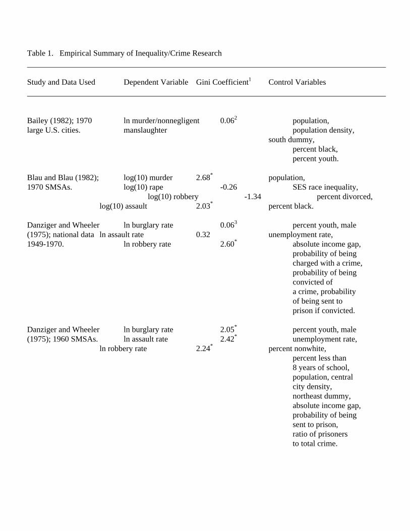
Table 1. Empirical Summary of Inequality/Crime Research
Study and Data Used Dependent Variable Gini Coefficient1 Control Variables
Bailey (1982); 1970 ln murder/nonnegligent 0.062 population,large U.S. cities. manslaughter population density, south dummy, percent black, percent youth.
Blau and Blau (1982); log(10) murder 2.68* population,1970 SMSAs. log(10) rape -0.26 SES race inequality, log(10) robbery -1.34 percent divorced, log(10) assault 2.03* percent black.
Danziger and Wheeler ln burglary rate 0.063 percent youth, male(1975); national data ln assault rate 0.32 unemployment rate,1949-1970. ln robbery rate 2.60* absolute income gap, probability of being charged with a crime,
probability of beingconvicted of
a crime, probability of being sent to prison if convicted.
Danziger and Wheeler ln burglary rate 2.05* percent youth, male(1975); 1960 SMSAs. ln assault rate 2.42* unemployment rate, ln robbery rate 2.24* percent nonwhite, percent less than 8 years of school, population, central city density, northeast dummy, absolute income gap, probability of being sent to prison, ratio of prisoners to total crime.
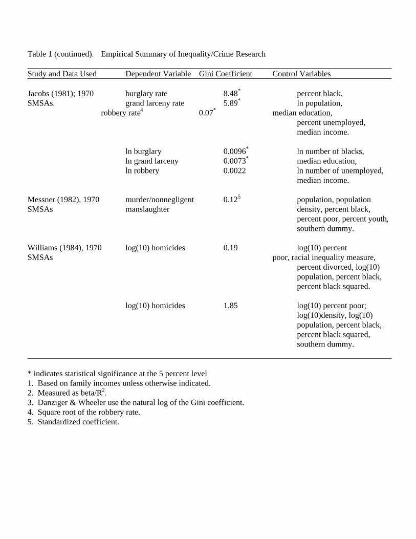
Table 1 (continued). Empirical Summary of Inequality/Crime Research
Study and Data Used Dependent Variable Gini Coefficient Control Variables
Jacobs (1981); 1970 burglary rate 8.48* percent black,SMSAs. grand larceny rate 5.89* ln population, robbery rate4 0.07* median education, percent unemployed, median income.
ln burglary 0.0096* ln number of blacks, ln grand larceny 0.0073* median education, ln robbery 0.0022 ln number of unemployed, median income. Messner (1982), 1970 murder/nonnegligent 0.125 population, populationSMSAs manslaughter density, percent black, percent poor, percent youth, southern dummy.
Williams (1984), 1970 log(10) homicides 0.19 log(10) percentSMSAs poor, racial inequality measure, percent divorced, log(10)
population, percent black, percent black squared.
log(10) homicides 1.85 log(10) percent poor;log(10)density, log(10) population, percent black,percent black squared,southern dummy.
* indicates statistical significance at the 5 percent level1. Based on family incomes unless otherwise indicated.2. Measured as beta/R2.3. Danziger & Wheeler use the natural log of the Gini coefficient.4. Square root of the robbery rate.5. Standardized coefficient.

Table 2. Inequality and Crime: Summary of EBA and OLS Results for 28 Major SMSAs:1975-1990
Crime Index Wage Betamin Betamax1 OLS Point T-Statistic(per 100,000) Inequality
Measure
Aggravated AssaultGini 419.75 1217.70 T 450.71 1.55*Mehran 220.75 999.31 T 268.57 1.11Piesch 521.60 1313.46 T 563.90 1.79*Bonferroni 289.57 1039.57 T 328.24 1.33*Covariation 0.99 2.61 T 1.32 1.44*Interquartile -39.40 586.97 66.82 0.36
Murder/Nonnegligent ManslaughterGini 4.29 39.57 T 20.21 2.23*Mehran -6.29 28.65 12.22 1.61*Piesch 12.09 46.33 T 28.09 2.55*Bonferroni -4.24 29.33 12.46 1.61*Covariation 0.028 0.094 T 0.043 1.50*Interquartile -18.14 8.13 -1.30 -0.22
Motor Vehicle TheftGini 528.58 2507.09 T 750.58 1.18Mehran 45.78 2001.50 T 363.11 0.68Piesch 820.59 2761.97 T 1007.06 1.45*Bonferroni 192.44 2075.15 T 484.46 0.89Covariation 1.27 5.18 T 2.12 1.05Interquartile -729.31 835.57 -325.87 -0.81
Larceny/TheftGini -329.37 6543.15 2202.82 1.40*Mehran -1378.87 5377.94 1268.66 0.97Piesch 393.53 7131.27 T 2783.78 1.63*Bonferroni -1356.92 5161.97 1155.40 0.86Covariation 5.41 18.34 T 9.01 1.81*Interquartile -2824.36 2370.04 -735.25 -0.74
Robbery Gini -384.69 1010.65 154.48 0.61Mehran -636.78 738.23 -2.46 -0.012Piesch -171.28 1190.02 268.92 0.98Bonferroni -617.24 707.82 -25.56 -0.12
Covariation 0.26 2.88 T 0.99 1.24Interquartile -701.26 338.78 -95.61 -0.60
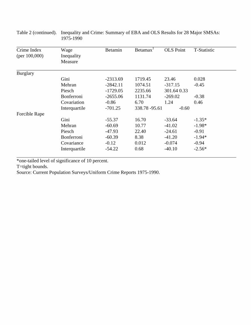
Table 2 (continued). Inequality and Crime: Summary of EBA and OLS Results for 28 Major SMSAs:1975-1990
Crime Index Wage Betamin Betamax1 OLS Point T-Statistic(per 100,000) Inequality
Measure
BurglaryGini -2313.69 1719.45 23.46 0.028Mehran -2842.11 1074.51 -317.15 -0.45Piesch -1729.05 2235.66 301.64 0.33Bonferroni -2655.06 1131.74 -269.02 -0.38Covariation -0.86 6.70 1.24 0.46Interquartile -701.25 338.78 -95.61 -0.60
Forcible RapeGini -55.37 16.70 -33.64 -1.35*Mehran -60.69 10.77 -41.02 -1.98*Piesch -47.93 22.40 -24.61 -0.91Bonferroni -60.39 8.38 -41.20 -1.94*Covariance -0.12 0.012 -0.074 -0.94Interquartile -54.22 0.68 -40.10 -2.56*
*one-tailed level of significance of 10 percent.T=tight bounds.Source: Current Population Surveys/Uniform Crime Reports 1975-1990.
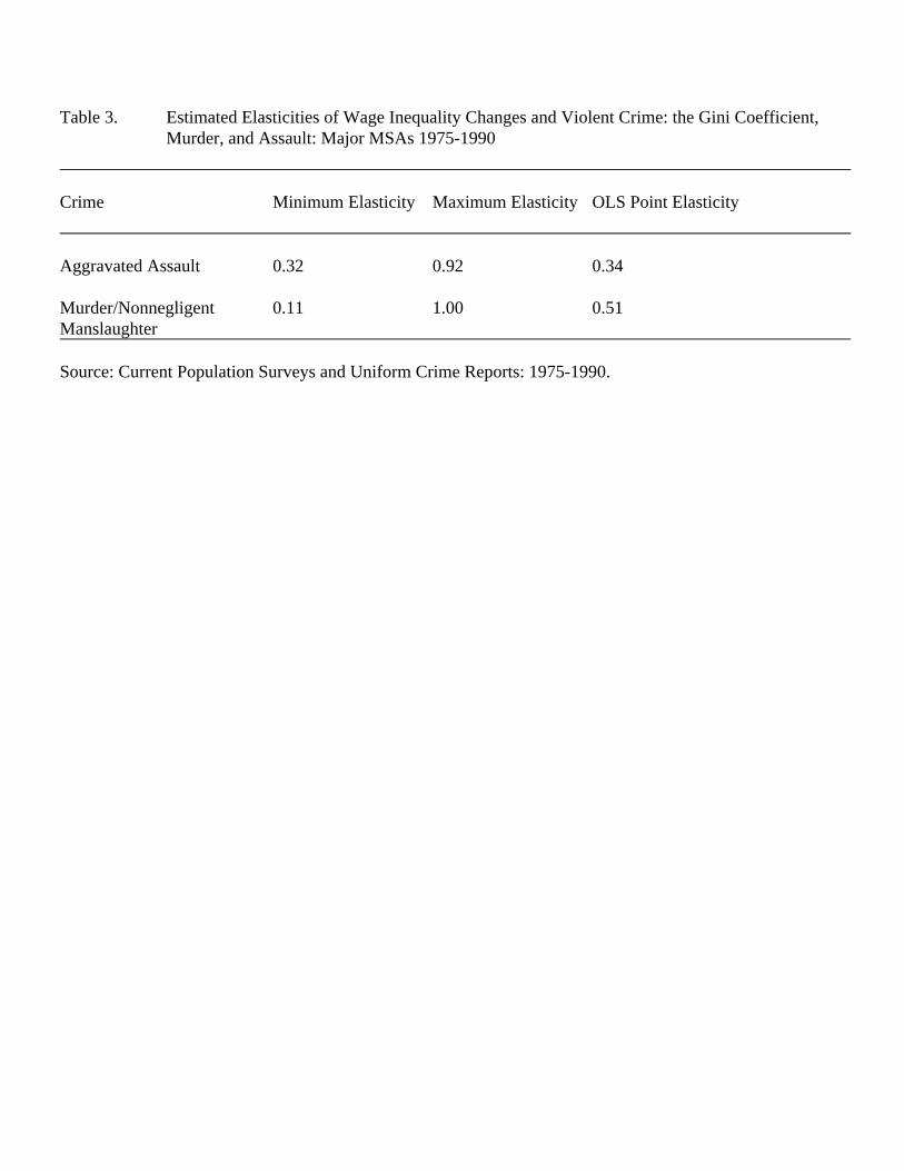
Table 3. Estimated Elasticities of Wage Inequality Changes and Violent Crime: the Gini Coefficient,Murder, and Assault: Major MSAs 1975-1990
Crime Minimum Elasticity Maximum Elasticity OLS Point Elasticity
Aggravated Assault 0.32 0.92 0.34
Murder/Nonnegligent 0.11 1.00 0.51Manslaughter
Source: Current Population Surveys and Uniform Crime Reports: 1975-1990.
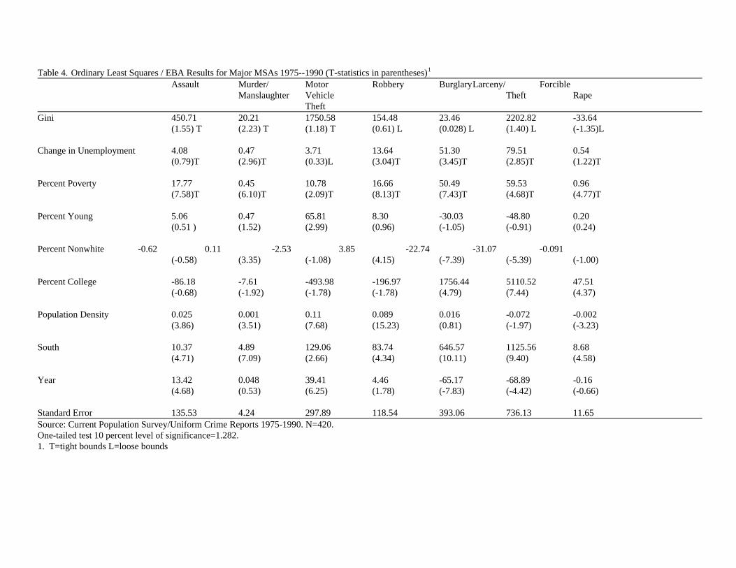
Table 4. Ordinary Least Squares / EBA Results for Major MSAs 1975--1990 (T-statistics in parentheses)1
Assault Murder/ Motor Robbery BurglaryLarceny/ ForcibleManslaughter Vehicle Theft Rape
TheftGini 450.71 20.21 1750.58 154.48 23.46 2202.82 -33.64
(1.55) T (2.23) T (1.18) T (0.61) L (0.028) L (1.40) L (-1.35)L
Change in Unemployment 4.08 0.47 3.71 13.64 51.30 79.51 0.54(0.79)T (2.96)T (0.33)L (3.04)T (3.45)T (2.85)T (1.22)T
Percent Poverty 17.77 0.45 10.78 16.66 50.49 59.53 0.96(7.58)T (6.10)T (2.09)T (8.13)T (7.43)T (4.68)T (4.77)T
Percent Young 5.06 0.47 65.81 8.30 -30.03 -48.80 0.20(0.51 ) (1.52) (2.99) (0.96) (-1.05) (-0.91) (0.24)
Percent Nonwhite -0.62 0.11 -2.53 3.85 -22.74 -31.07 -0.091(-0.58) (3.35) (-1.08) (4.15) (-7.39) (-5.39) (-1.00)
Percent College -86.18 -7.61 -493.98 -196.97 1756.44 5110.52 47.51(-0.68) (-1.92) (-1.78) (-1.78) (4.79) (7.44) (4.37)
Population Density 0.025 0.001 0.11 0.089 0.016 -0.072 -0.002(3.86) (3.51) (7.68) (15.23) (0.81) (-1.97) (-3.23)
South 10.37 4.89 129.06 83.74 646.57 1125.56 8.68(4.71) (7.09) (2.66) (4.34) (10.11) (9.40) (4.58)
Year 13.42 0.048 39.41 4.46 -65.17 -68.89 -0.16(4.68) (0.53) (6.25) (1.78) (-7.83) (-4.42) (-0.66)
Standard Error 135.53 4.24 297.89 118.54 393.06 736.13 11.65Source: Current Population Survey/Uniform Crime Reports 1975-1990. N=420.One-tailed test 10 percent level of significance=1.282.1. T=tight bounds L=loose bounds