Changes in College Enrollment and Wage Inequality:

Distinguishing Price and Composition Effects

Pedro Carneiro and Sokbae Lee∗

University College London, Institute for Fiscal Studiesand Centre for Microdata Methods and Practice

December 2007

Abstract

Increases in college enrollment cause changes in the distribution of ability among college and highschool graduates. This paper estimates a semiparametric selection model of schooling and wages toshow that, for fixed skill prices, a 14% increase in college participation (analogous to the increaseobserved in the 1980s), reduces the college premium by 12% and increases the 90-10 percentile ratioamong college graduates by 2%. The semiparametric method we use is new and it extends themethod of local instrumental variables developed by Heckman and Vytlacil (1999, 2001, 2005) tothe estimation of not only means, but also distributions of potential outcomes.

Keywords: Comparative advantage, composition effects, local instrumental variables, marginal treat-ment effect, semiparametric estimation, wage inequality.

JEL classification codes: C14; C31; J31.

∗Corresponding address: Department of Economics, University College London, London, WC1E 6BT, UK; emails:p.carneiro@ucl.ac.uk (Carneiro) and l.simon@ucl.ac.uk (Lee). We thank an editor, an associate editor, and three anonymousreferees for helpful comments. We also thank participants in numerous seminars for useful comments, especially RitaAlmeida, Joe Altonji, David Autor, Richard Blundell, Olympia Bover, Peter Gottschalk, Alan Krueger, Alan Manning,Costas Meghir, Steve Pischke and Tom Stoker. This research is supported in part by the Economic and Social ResearchCouncil (ESRC) Research Grant RES-000-22-2542. We thank the Leverhulme Trust and ESRC (RES-589-28-0001) throughthe funding of the Centre for Microdata Methods and Practice (Carneiro and Lee) and of the research programme Evidence,Inference and Inquiry (Lee). Carneiro also thanks the Poverty Unit of the World Bank Research Group and Georgetownfor their hospitality.

1 Introduction

College enrollment doubled from 30% to 60% between 1960 and 2000. Such a large increase in college

enrollment rates is bound to cause changes in the quality of college and high school workers. As a

result, we cannot compare measures of the college premium and within group inequality across different

periods. Trends in the college premium and wage inequality confound changes in prices and changes in

composition, and it is important to separate the two.

The goal of this paper is to uncover the empirical magnitude of this problem, generally called compo-

sition effect. In order to do so, we estimate a semiparametric model of heterogeneous agents self-selecting

into college, and uncover the magnitude of selection observed in the data.1 We use the resulting estimates

to characterize the distributions of wages for individuals enrolling either in college or in high school at

a given point in time, and how they change in response to changes in college enrollment. We find that

an increase of 14% in the proportion of college-goers (of similar magnitude to the one observed in the

1980s) leads to: i) a reduction of 12% in the college premium; ii) a 2% increase in the ratio of the 90th

to the 10th percentile (P90-P10) of the college wage distribution; iii) and no change in the P90-P10 ratio

of the high school wage distribution.

We use data from the National Longitudinal Survey of Youth of 1979 (NLSY79). The reason why

we focus on this dataset instead of the Census or Current Population Survey (CPS) is because of our

emphasis of heterogeneity. The NLSY79 is rich on observed measures of heterogeneity (unavailable in

either the Census or the CPS), and on the potential to construct instrumental variables for schooling

(the standard ones in the literature) which allow us to account for unobserved heterogeneity.

Unfortunately, the NLSY79 surveys only a fixed set of cohorts, and most of the reliable wage data we

are comfortable using is from the 1990s (because of the young age of the respondents in the 1980s).2 This

limitation of the data does not invalidate our exercise. Suppose we want to study the effects of changes

in composition in the 1980s. In order to do so, we need to keep skill prices fixed, so that all fluctuations

in wages can be attributed to changes in the distribution of worker quality. One alternative is to take

1980 prices as fixed and simulate an increase in college enrollment analogous to the one observed in the

1980s. However, an equally valid alternative is to fix prices at their 1990s values, and use them to value

changes in composition similar to the ones occurring in the 1980s. We adopt the latter procedure.1One measure of the importance of selection is, say, the OLS-IV gap in estimates of the returns to schooling. As discussed

in Card (2001), the usual finding is that instrumental variables (IV) estimates of the return to one year of schooling areabove ordinary least squares (OLS) estimates of the same parameter by 2 to 3 percentage points (corresponding to 25 to50% of the size of the OLS coefficient). Much of the literature on inequality studies the evolution of the college premium,estimated as the difference in log wages of individuals with 12 and 16 years of education. If we extrapolated the reportedOLS-IV gap to four years of schooling we would get something on the order of 8-12% percentage points. This correspondsto roughly 20 to 25% of the college premium in 1980, and almost 40 to 50% of its increase in between 1980 and 1990 (Katzand Murphy, 1992).

2The NLSY79 labor market data is representative of the US labor market for the relevant cohorts and periods of thesurvey. It replicates the evolution of the wage structure in the 1990s for these cohorts, as measured by the CPS.

1

We estimate a very flexible specification of our empirical model. Building on the work of Heckman

and Vytlacil (1999, 2001, 2005) and Das, Newey and Vella (2003), we put minimal structure on the

specification of the schooling decision and wage determination, and also on the specification of observed

and unobserved heterogeneity. Then we use our estimates to carry out simulations to quantify the effect

of changes in college enrollment, keeping skill prices fixed.

We also make two new contributions to the econometrics literature: first, we show how to extend

the method of local instrumental variables of Heckman and Vytlacil (1999, 2001, 2005) to identify the

distributions of potential outcomes;3 second, we develop a semiparametric method for estimating the

entire marginal distributions of potential outcomes.

Our results have applications beyond the one on which we focus. Distributions of potential outcomes

are useful for policy makers who care about distributional effects of policies. To our best knowledge,

estimation of marginal distributions of potential outcomes has been considered by Imbens and Rubin

(1997) and Abadie (2002, 2003).4 However, these three papers develop estimators under the local average

treatment effect (LATE) framework of Imbens and Angrist (1994). They are useful for evaluating

the effects of polices in place, but not for forecasting those of new polices. One could estimate a

structural econometric model that describes individual choices and corresponding outcomes to predict

the distributional effects of new polices, but this would involve stringent parametric and functional-form

assumptions on the econometric model. In this paper, we provide an alternative method that can be used

to evaluate the distributional effect of a new policy without specifying a complete parametric model.

Moreover, since quantile treatment effects are defined as the differences between quantiles of marginal

distributions of potential outcomes, we also contribute to the literature on quantile treatment effects

and on instrumental variables estimation of quantile regression models.5

We use the model primarily to characterize the pattern of sorting of individuals across schooling levels,

and the importance of composition effects. However, the model also allows us to revisit the work of Chay

and Lee (2000) and Taber (2001) and assess the role of changes in selection bias (keeping composition

fixed) on wage inequality. The questions these two papers address are fundamentally different from

ours. The authors try to keep composition fixed, and then ask how selection bias has changed over time

because of changes in the price of unobserved ability. Taber (2001) suggests that the observed rise in

the college premium in the 1980s is just a reflection of the increase in the return to unobserved ability,

although Chay and Lee (2000) argue that the latter can account at most for 30 to 40% of the increase3See Heckman, Urzua, and Vytlacil (2006) for extensions of the method of local instrumental variables. See also Aakvik,

Heckman, and Vytlacil (2005) for the analysis of the latent variable framework of Heckman and Vytlacil (1999, 2001, 2005)using factor structures.

4A recent working paper by Chen and Khan (2007) develops estimators of the scale ratio between potential outcomesunder some symmetry conditions on the joint distribution of outcome and selection errors.

5Some recent papers in this literature include: Abadie, Angrist, and Imbens (2002), Chesher (2003), Imbens and Newey(2003), Chernozhukov and Hansen (2005, 2006), Chernozhukov, Imbens, and Newey (2007), Ma and Koenker (2006), Lee(2006), and Horowitz and Lee (2007) among others.

2

in the college premium. In a recent paper, Deschenes (2006) also argues that most of the increase in the

college premium is due to an increase in the return to schooling, not in the return to ability. Using our

model we update the analysis of Taber (2001) to the 1990s. We show that the commonly used measure

of college premium cannot reveal the true evolution of skill prices.

The literature on wage inequality is too large to be summarized here. Most empirical papers in this

literature recognize the problem we address, but often the prior is that they are empirically unimportant

(see, for example, Katz and Murphy, 1992, Juhn, Murphy and Pierce, 1993, Katz and Autor, 1999,

Card and Lemieux, 2001, Acemoglu, 2002, Autor, Katz and Kearney, 2007). In contrast, changes in

composition are a crucial ingredient of Galor and Moav’s (2001) model of technological change and wage

inequality. Similarly, Gosling, Machin and Meghir (2000) find that cohort effects are the main driving

force of wage inequality in the UK, and suggest that shifts in composition may explain part of the

differences across cohorts. Very few papers have tackled this issue directly. One example is Juhn, Kim

and Vella (2005) who, using data from the Census, find that college quality declines as college enrollment

increases, but that such fluctuations are unimportant to explain changes in the college premium. Using

the Census but a different methodology, Carneiro and Lee (2007) find evidence of composition effects

consistent with the ones reported in this paper, and show how they affect the trend in the college and

age premia in the last 40 years.

Also related are recent papers by Moffitt (2007) and Carneiro, Heckman and Vytlacil (2007) esti-

mating the amount of heterogeneity in the returns to schooling. Starting from a similar model (which is

the same we use in this paper), but using different econometric methods and data, both papers estimate

that as the proportion of individuals in college rises the average return to college for those enrolled in

college is bound to fall. We add to these not only by focusing on levels of wages in college and high

school (as opposed to returns), but also by estimating counterfactual distributions of wages for each level

of schooling.

The remainder of this paper is organized as follows. In section 2 we present a simple econometric

model which underlies our empirical work. In section 3, we describe the basic ideas behind a semi-

parametric estimation procedure based on Section 2, and in section 4 we describe in detail the way we

apply it. Secion 5 presents asymptotic distributions for our estimators. The data we use are described

in Section 6. In section 7 we apply our model to the study of wage inequality using white males in

the NLSY. Using our estimates we document the patterns of sorting of individuals to different levels of

schooling and the empirical importance of selection bias and composition effects. Section 8 gives some

concluding remarks. In the Appendix we provide a detailed description of the data and our estimation

procedure.

3

2 The Econometric Model and Identification of Potential Out-come Distributions

The econometric model we consider is that of Heckman and Vytlacil (1999, 2001, 2005).6 Let Y1 and Y0

be potential individual outcomes in two states, 1 and 0. In this paper, Y1 is the log college wage and Y0

is the log high school wage, as in Willis and Rosen (1979).

We assume

(2.1) Y1 = µ1 (X,U1) and Y0 = µ0 (X, U0) ,

where X is a vector of observed random variables influencing potential outcomes, µ1 and µ0 are unknown

functions, and U1 and U0 are unobserved random variables.

We assume that individuals choose to be in state 1 or 0 (prior to the realizations of the outcomes of

interest) according to the following equation:

(2.2) S = 1 if µS (Z)− US > 0,

where Z is a vector of observed random variables influencing the decision equation, µS is an unknown

function of Z, and US is an unobserved random variable. In this paper, equation (2.2) can be interpreted

as the reduced form of an economic model of college attendance.7 The advantage of specifying it this

way is the relatively little structure it imposes on the model. In particular, Vytlacil (2002) shows that

the independent and monotonicity assumptions needed to interpret instrumental variables estimates in a

model of heterogeneous returns (e.g., Imbens and Angrist, 1994) imply that the data can be rationalized

with the model of equations (2.1) and (2.2) (as long as one does not impose parametric functional forms

and distributional assumptions on the model). This result guarantees that our model is consistent with

the IV estimates of the returns to college that can be produced in our data.

For each individual, the observed outcome Y is

Y = SY1 + (1− S)Y0.

The set of variables in X can be a subset of Z. For identification, assume that there is at least one

variable in Z that is not in X (exclusion restriction). As in Heckman and Vytlacil (2001,2005), we can

rewrite (2.2) as:

S = 1 if P > V,

where V = FUS |X,Z [US |X,Z], P = FUS |X,Z [µS(Z)|X, Z], and FUS |X,Z(us|x, z) is the CDF of US condi-

tional on X = Z and Z = z. For any arbitrary distribution of US conditional on X and Z, by definition,

V ∼ Unif [0, 1] conditional on X and Z.6For example, see Section 2 of Heckman and Vytlacil (2005).7Carneiro, Heckman and Vytlacil (2007) use this model to study heterogeneity in the returns to college and present an

economic model that can justify the specification in (2.2).

4

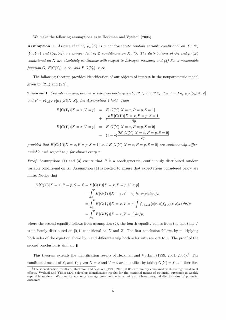
We make the following assumptions as in Heckman and Vytlacil (2005).

Assumption 1. Assume that (1) µS(Z) is a nondegenerate random variable conditional on X; (2)

(U1, US) and (U0, US) are independent of Z conditional on X; (3) The distributions of US and µS(Z)

conditional on X are absolutely continuous with respect to Lebesgue measure; and (4) For a measurable

function G, E|G(Y1)| < ∞, and E|G(Y0)| < ∞.

The following theorem provides identification of our objects of interest in the nonparametric model

given by (2.1) and (2.2).

Theorem 1. Consider the nonparametric selection model given by (2.1) and (2.2). Let V = FUS |X,Z [US |X,Z]

and P = FUS |X,Z [µS(Z)|X, Z]. Let Assumption 1 hold. Then

E [G(Y1)|X = x, V = p] = E [G(Y )|X = x, P = p, S = 1]

+ p∂E [G(Y )|X = x, P = p, S = 1]

∂p

E [G(Y0)|X = x, V = p] = E [G(Y )|X = x, P = p, S = 0]

− (1− p)∂E [G(Y )|X = x, P = p, S = 0]

∂p

provided that E [G(Y )|X = x, P = p, S = 1] and E [G(Y )|X = x, P = p, S = 0] are continuously differ-

entiable with respect to p for almost every x.

Proof. Assumptions (1) and (3) ensure that P is a nondegenerate, continuously distributed random

variable conditional on X. Assumption (4) is needed to ensure that expectations considered below are

finite. Notice that

E [G(Y )|X = x, P = p, S = 1] = E [G(Y )|X = x, P = p, V < p]

=∫ p

0

E [G(Y1)|X = x, V = v] fV |X(v|x)dv/p

=∫ p

0

E [G(Y1)|X = x, V = v]∫

fV |X,Z(v|x, z)fZ|X(z|x)dz dv/p

=∫ p

0

E [G(Y1)|X = x, V = v] dv/p,

where the second equality follows from assumption (2), the fourth equality comes from the fact that V

is uniformly distributed on [0, 1] conditional on X and Z. The first conclusion follows by multiplying

both sides of the equation above by p and differentiating both sides with respect to p. The proof of the

second conclusion is similar.

This theorem extends the identification results of Heckman and Vytlacil (1999, 2001, 2005).8 The

conditional means of Y1 and Y0 given X = x and V = v are identified by taking G(Y ) = Y and therefore8The identification results of Heckman and Vytlacil (1999, 2001, 2005) are mainly concerned with average treatment

effects. Vytlacil and Yildiz (2007) develop identification results for the marginal means of potential outcomes in weaklyseparable models. We identify not only average treatment effects but also whole marginal distributions of potentialoutcomes.

5

the marginal treatment effect (MTE), defined as E (Y1 − Y0|X = x, V = v), is identified. Furthermore,

the conditional distributions of Y1 and Y0 given X = x and V = v are identified by choosing G(Y ) =

1(Y ≤ y), where 1(·) is the standard indicator function, and therefore the conditional densities and

quantiles are also identified.

Notice that we can only identify E [G(Y1)|X = x, V = p] over the support of P for individuals in

S = 1 conditional on X = x, and E ([G(Y0)|X = x, V = p] over the support of P for individuals in S = 0

conditional on X = x. As a consequence, we can only identify the MTE over the common support of P

for individuals in S = 1 and S = 0 conditional on X = x.

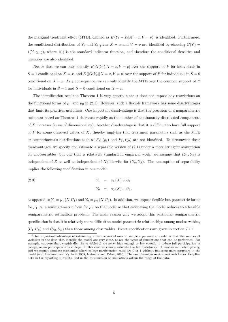
The identification result in Theorem 1 is very general since it does not impose any restrictions on

the functional forms of µ1 and µ0 in (2.1). However, such a flexible framework has some disadvantages

that limit its practical usefulness. One important disadvantage is that the precision of a nonparametric

estimator based on Theorem 1 decreases rapidly as the number of continuously distributed components

of X increases (curse of dimensionality). Another disadvantage is that it is difficult to have full support

of P for some observed values of X, thereby implying that treatment parameters such as the MTE

or counterfactuals distributions such as FY1 (y1) and FY0 (y0) are not identified. To circumvent these

disadvantages, we specify and estimate a separable version of (2.1) under a more stringent assumption

on unobservables, but one that is relatively standard in empirical work: we assume that (U1, US) is

independent of Z as well as independent of X; likewise for (U0, US). The assumption of separability

implies the following modification in our model:

Y1 = µ1 (X) + U1(2.3)

Y0 = µ0 (X) + U0,

as opposed to Y1 = µ1 (X, U1) and Y0 = µ0 (X, U0). In addition, we impose flexible but parametric forms

for µ1, µ0 a semiparametric form for µS on the model so that estimating the model reduces to a feasible

semiparametric estimation problem. The main reason why we adopt this particular semiparametric

specification is that it is relatively more difficult to model parametric relationships among unobservables,

(U1, US) and (U0, US) than those among observables. Exact specifications are given in section 7.1.9

9One important advantage of estimating a flexible model over a complete parametric model is that the sources ofvariation in the data that identify the model are very clear, as are the types of simulations that can be performed. Forexample, suppose that, empirically, the variables Z are never high enough or low enough to induce full participation incollege, or no participation in college. In this case we cannot estimate the full distribution of unobserved heterogeneity,and we cannot simulate economies where college participation rates are 0 or 1 without imposing more structure in themodel (e.g., Heckman and Vytlacil, 2005, Ichimura and Taber, 2000). The use of semiparametric methods forces disciplineboth in the reporting of results, and in the construction of simulations within the range of the data.

6

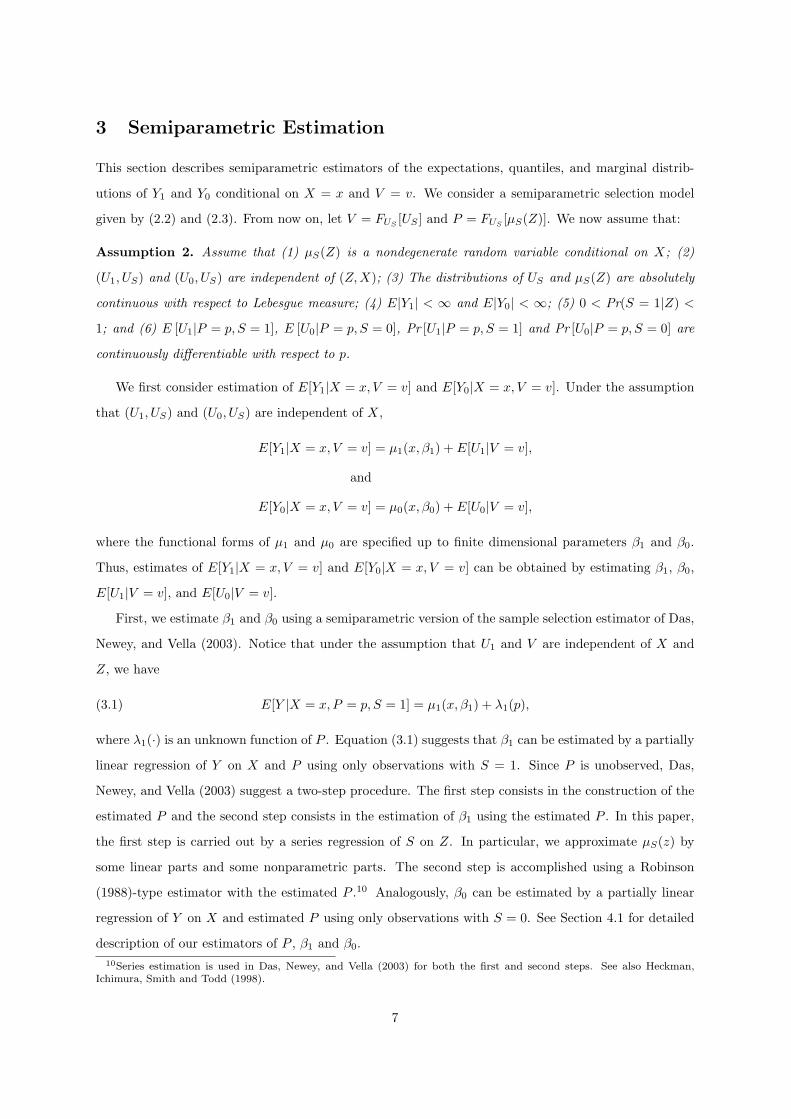
3 Semiparametric Estimation

This section describes semiparametric estimators of the expectations, quantiles, and marginal distrib-

utions of Y1 and Y0 conditional on X = x and V = v. We consider a semiparametric selection model

given by (2.2) and (2.3). From now on, let V = FUS [US ] and P = FUS [µS(Z)]. We now assume that:

Assumption 2. Assume that (1) µS(Z) is a nondegenerate random variable conditional on X; (2)

(U1, US) and (U0, US) are independent of (Z, X); (3) The distributions of US and µS(Z) are absolutely

continuous with respect to Lebesgue measure; (4) E|Y1| < ∞ and E|Y0| < ∞; (5) 0 < Pr(S = 1|Z) <

1; and (6) E [U1|P = p, S = 1], E [U0|P = p, S = 0], Pr [U1|P = p, S = 1] and Pr [U0|P = p, S = 0] are

continuously differentiable with respect to p.

We first consider estimation of E[Y1|X = x, V = v] and E[Y0|X = x, V = v]. Under the assumption

that (U1, US) and (U0, US) are independent of X,

E[Y1|X = x, V = v] = µ1(x, β1) + E[U1|V = v],

and

E[Y0|X = x, V = v] = µ0(x, β0) + E[U0|V = v],

where the functional forms of µ1 and µ0 are specified up to finite dimensional parameters β1 and β0.

Thus, estimates of E[Y1|X = x, V = v] and E[Y0|X = x, V = v] can be obtained by estimating β1, β0,

E[U1|V = v], and E[U0|V = v].

First, we estimate β1 and β0 using a semiparametric version of the sample selection estimator of Das,

Newey, and Vella (2003). Notice that under the assumption that U1 and V are independent of X and

Z, we have

(3.1) E[Y |X = x, P = p, S = 1] = µ1(x, β1) + λ1(p),

where λ1(·) is an unknown function of P . Equation (3.1) suggests that β1 can be estimated by a partially

linear regression of Y on X and P using only observations with S = 1. Since P is unobserved, Das,

Newey, and Vella (2003) suggest a two-step procedure. The first step consists in the construction of the

estimated P and the second step consists in the estimation of β1 using the estimated P . In this paper,

the first step is carried out by a series regression of S on Z. In particular, we approximate µS(z) by

some linear parts and some nonparametric parts. The second step is accomplished using a Robinson

(1988)-type estimator with the estimated P .10 Analogously, β0 can be estimated by a partially linear

regression of Y on X and estimated P using only observations with S = 0. See Section 4.1 for detailed

description of our estimators of P , β1 and β0.10Series estimation is used in Das, Newey, and Vella (2003) for both the first and second steps. See also Heckman,

Ichimura, Smith and Todd (1998).

7

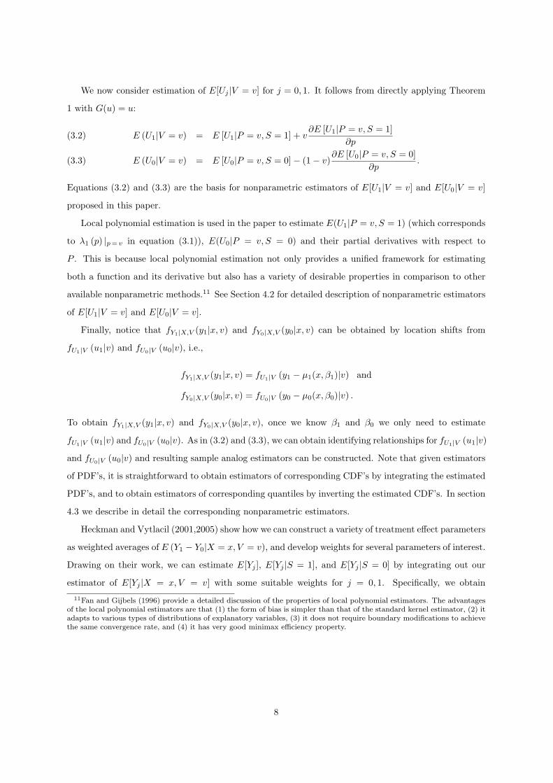
We now consider estimation of E[Uj |V = v] for j = 0, 1. It follows from directly applying Theorem

1 with G(u) = u:

E (U1|V = v) = E [U1|P = v, S = 1] + v∂E [U1|P = v, S = 1]

∂p(3.2)

E (U0|V = v) = E [U0|P = v, S = 0]− (1− v)∂E [U0|P = v, S = 0]

∂p.(3.3)

Equations (3.2) and (3.3) are the basis for nonparametric estimators of E[U1|V = v] and E[U0|V = v]

proposed in this paper.

Local polynomial estimation is used in the paper to estimate E(U1|P = v, S = 1) (which corresponds

to λ1 (p) |p = v in equation (3.1)), E(U0|P = v, S = 0) and their partial derivatives with respect to

P . This is because local polynomial estimation not only provides a unified framework for estimating

both a function and its derivative but also has a variety of desirable properties in comparison to other

available nonparametric methods.11 See Section 4.2 for detailed description of nonparametric estimators

of E[U1|V = v] and E[U0|V = v].

Finally, notice that fY1|X,V (y1|x, v) and fY0|X,V (y0|x, v) can be obtained by location shifts from

fU1|V (u1|v) and fU0|V (u0|v), i.e.,

fY1|X,V (y1|x, v) = fU1|V (y1 − µ1(x, β1)|v) and

fY0|X,V (y0|x, v) = fU0|V (y0 − µ0(x, β0)|v) .

To obtain fY1|X,V (y1|x, v) and fY0|X,V (y0|x, v), once we know β1 and β0 we only need to estimate

fU1|V (u1|v) and fU0|V (u0|v). As in (3.2) and (3.3), we can obtain identifying relationships for fU1|V (u1|v)

and fU0|V (u0|v) and resulting sample analog estimators can be constructed. Note that given estimators

of PDF’s, it is straightforward to obtain estimators of corresponding CDF’s by integrating the estimated

PDF’s, and to obtain estimators of corresponding quantiles by inverting the estimated CDF’s. In section

4.3 we describe in detail the corresponding nonparametric estimators.

Heckman and Vytlacil (2001,2005) show how we can construct a variety of treatment effect parameters

as weighted averages of E (Y1 − Y0|X = x, V = v), and develop weights for several parameters of interest.

Drawing on their work, we can estimate E[Yj ], E[Yj |S = 1], and E[Yj |S = 0] by integrating out our

estimator of E[Yj |X = x, V = v] with some suitable weights for j = 0, 1. Specifically, we obtain

11Fan and Gijbels (1996) provide a detailed discussion of the properties of local polynomial estimators. The advantagesof the local polynomial estimators are that (1) the form of bias is simpler than that of the standard kernel estimator, (2) itadapts to various types of distributions of explanatory variables, (3) it does not require boundary modifications to achievethe same convergence rate, and (4) it has very good minimax efficiency property.

8

estimators of E[Yj ], E[Yj |S = 1], and E[Yj |S = 0] by the sample analogs of the following formulae:

E[Yj ] =∫ ∫ 1

0

E[Yj |X = x, V = v]fX(x) dv dx,

E[Yj |S = 1] =∫ ∫ 1

0

E[Yj |X = x, V = v]1− FP |X(v|x)

Pr(S = 1)fX(x) dv dx,

and

E[Yj |S = 0] =∫ ∫ 1

0

E[Yj |X = x, V = v]FP |X(v|x)Pr(S = 0)

fX(x) dv dx.

(3.4)

for j = 0, 1. See Appendix B.1 for details on implementing (3.4). Using estimates of these conditional

expectations, standard treatment effect parameters can be estimated: ATE = E[Y1] − E[Y0], TT =

E[Y1|S = 1]− E[Y0|S = 1], TUT = E[Y1|S = 0]− E[Y0|S = 0], and OLS = E[Y1|S = 1]− E[Y0|S = 0].

E[Y1|S = 1] and E[Y0|S = 0] can also be estimated directly by taking sample means of observed college

and high school wages. Therefore, comparison between model-based and direct estimates of E[Y1|S = 1]

and E[Y0|S = 0] provides a goodness-of-fit check of our model.

Similarly, integrating our estimators of fYj |X,V (yj |x, v) for j = 0, 1 with the weights in (3.4), we can

obtain estimators of fYj (·), fYj |S=1(·|S = 1), and fYj |S=0(·|S = 0) for j = 0, 1. Note that fY1|S=1(·|S = 1)

and fY0|S=0(·|S = 0) can also be estimated directly by taking sample analogs of observed college and

high school wages, which again allows us to do a goodness-of-fit check of our model.

4 Details of Estimation Procedure

4.1 Estimating P , β1 and β0

This section provides a detailed description of our estimators of P , β1 and β0. Assume that the data

consist of i.i.d. observations (Yi, Si, Xi, Zi) : i = 1, . . . , n. First, we consider series estimation of P .

In Section 3, P = FUS[µS(Z)] = Pr(S = 1|Z). In order to avoid the curse of dimensionality, we model

Pr(S = 1|Z = z) as a partially linear additive regression model:

Pr(S = 1|Z = z) = ϕ1(z1) + . . . + ϕd(zd) + z′pcϑ,(4.1)

where z = (zc, zpc), zc = (z1, . . . , zd)′ is a d-dimensional vector of continuous random variables (non-

parametric components), zpc is a vector of parametric components, ϕ1, . . . , ϕd are unknown functions,

and ϑ is a vector of unknown parameters. The partially linear additive structure in (4.1) is adopted to

have a good precision in our estimation procedure. In our empirical application, Zc includes AFQT,

college tuition at age 17, and unemployment rates at age 17.

To describe the series estimator, let pk : k = 1, 2, . . . denote a basis for real-valued smooth functions

defined on R such that a linear combination of pk : k = 1, 2, . . . can approximate ϕj(·) for each

j = 1, . . . , d as the number of approximating functions increases to infinity. For any positive integer κ,

9

define

Pκ(z) = [p1(z1), . . . , pκ(z1), . . . , p1(zd), . . . , pκ(zd), zpc]′.

Then for each i, the series estimator of P (Zi) is

P (Zi) = Pκ(Zi)′θnκ,

where

θnκ =

[n∑

i=1

Pκ(Zi)Pκ(Zi)′]−1 [

n∑

i=1

Pκ(Zi)Si

].

In finite samples, estimated P (Zi)’s might be negative or larger than one. To solve this, our estimator

is a trimmed version:

P (Zi) = P (Zi) + (1− δ − P (Zi))1(P (Zi) > 1) + (δ − P (Zi))1(P (Zi) < 0)(4.2)

for sufficiently small δ.

We now consider estimation of β1 and β0. For convenience, we assume linear-in-parameters forms for

µ1 and µ0, that is µj(x, βj) = µj(x)′βj for each j = 0, 1. Then β1 and β0 are estimated as in Robinson

(1988) (using the estimated rather than the true P ) with the S = 1 subsample and the S = 0 subsample,

respectively. Specifically, for j = 0, 1,

βj =

[n∑

i=1

Wji

µj(Xi)− Eh

[µj(Xi)

∣∣∣P (Zi),Wji

]µj(Xi)− Eh

[µj(Xi)

∣∣∣P (Zi),Wji

]′]−1

×[

n∑

i=1

Wji

µj(Xi)− Eh

[µj(Xi)

∣∣∣P (Zi),Wji

]Yi − Eh

[Yi

∣∣∣P (Zi),Wji

]],

(4.3)

where Wji = (Si)1(j=1)(1 − Si)1(j=0) and Eh[·|·] denotes the kernel mean regression estimator with a

bandwidth h. Alternatively, one could consider Wn,ji = (Si)1(j=1)(1−Si)1(j=0)ωn,ji, where ωn,ji is some

trimming function.

4.2 Estimating E[U1|V = v] and E[U0|V = v]

This section gives a detailed description of nonparametric estimators of E[U1|V = v] and E[U0|V = v].

First consider local polynomial estimation of E[U1|V = v]. In general, use of higher order polynomials

may reduce the bias but increase the variance by introducing more parameters. Fan and Gijbels (1996)

suggest that the order π of polynomial be equal to π = µ + 1, where µ is the order of the derivative

of the function of interest. That is, Fan and Gijbels (1996) recommend a local linear estimator for

fitting a function and a local quadratic estimator for fitting a first-order derivative. Following their

suggestions, E(U1|P = v, S = 1) is estimated by a local linear estimator using observations with S = 1

and ∂E(U1|P = v, S = 1)/∂p is estimated by a local quadratic estimator.

10

To be more specific, let (U1i, Pi, Si) : i = 1, . . . , n denote observations of estimated U1 and P along

with S, where U1i = Yi − µ1(Xi, β1) for i = 1, . . . , n. The local linear estimator E(U1|P = v, S = 1) is

obtained by solving the problem

minc0,c1

n∑

i=1

Si

[U1i − c0 − c1(Pi − v)

]2

K

(Pi − v

hn1

),

where K(·) is a kernel function and hn1 is a bandwidth. The resulting value of c0 is the local linear

estimator of E(U1|P = v, S = 1). Similarly, the local quadratic estimator ∂E(U1|P = v, S = 1)/∂p is

obtained by solving the problem

minc0,c1,c2

n∑

i=1

Si

[U1i − c0 − c1(Pi − v)− c2(Pi − v)2

]2

K

(Pi − v

hn2

),

where hn2 is a bandwidth that can be different from hn1. The resulting value of c1 is the local quadratic

estimator of ∂E(U1|P = v, S = 1)/∂p. Then the estimator of E[U1|V = v] is given by

E[U1|V = v] = v∂

∂pE(U1|P = v, S = 1) + E(U1|P = v, S = 1).(4.4)

Similarly, the estimator of E[U0|V = v] can be obtained by replacing unknown functions in the right

hand side of (3.3) with their nonparametric estimators.

4.3 Estimating f(u1|v) and f(u0|v)

This section describes nonparametric estimators of f(u1|v) and f(u0|v). As in (3.2) and (3.3), an

application of Theorem 1 yields the following relationships

fU1|V (u1|v) = fU1|P,S=1(u1|v, S = 1) + v∂

∂pfU1|P,S=1(u1|v, S = 1) and(4.5)

fU0|V (u0|v) = fU0|P,S=0(u0|v, S = 0)− (1− v)∂

∂pfU0|P,S=0(u0|v, S = 0).(4.6)

Sample analogs of the right-hand sides of equations (4.5) and (4.6) can be obtained by some suitable

nonparametric estimators.

We only discuss estimation of f (u1|v) in detail, since estimation of f (u0|v) is similar. To develop an

estimator of f (u1|v) using the equation (4.5), it is necessary to estimate fU1|P,S=1(u1|p, S = 1) and its

derivative with respect to p. Specifically, the estimator of f (u1|v) can be obtained by

f(u1|v) = v∂

∂pfU1|P,S=1(u1|v, S = 1) + fU1|P,S=1(u1|v, S = 1),(4.7)

where fU1|P,S=1(u1|v, S = 1) and ∂fU1|P,S=1(u1|v, S = 1)/∂p are defined below.

In order to compute fU1|P,S=1(u1|v, S = 1) and ∂fU1|P,S=1(u1|v, S = 1)/∂p in (4.7), we begin with

estimated data (U1i, Pi) : i = 1, . . . , n, Si = 1, where U1i = Yi − µ1(Xi, β1). One could estimate the

conditional density of U1 given P and its derivative by estimating the joint and marginal densities of

11

each variable using the standard kernel density estimators, taking the ratio between them to estimate

the conditional density, and finally computing a derivative of the conditional density. This procedure

would yield consistent estimators but it is quite cumbersome. Instead we use a direct method of Fan,

Yao, and Tong (1996), who develop local polynomial estimators of the conditional density function and

its derivative. To motivate the estimators of Fan, Yao, and Tong (1996), notice that, as δn → 0,

E

[δ−1n K

(U1 − u1

δn

) ∣∣∣∣P = v, S = 1]≈ fU1|P,S=1(u1|v, S = 1)

≈ fU1|P,S=1(u1|v0, S = 1) +∂

∂pfU1|P,S=1(u1|v0, S = 1)(v − v0)

for any v in a neighborhood of v0, where K is a nonnegative density function and δn is a bandwidth. This

suggests that the local linear estimator of fU1|P,S=1(u1|v, S = 1) can be defined as fU1|P,S=1(u1|v, S =

1) ≡ c0, where (c0, c1) solves the problem

(4.8) minc0,c1

n∑

i=1

Si

[δ−1n K

(U1i − u1

δn

)− c0 − c1(Pi − v)

]2

K

(Pi − v

hn1

),

and the local quadratic estimator of ∂fU1|P,S=1(u1|v, S = 1)/∂p can be defined as ∂fU1|P,S=1(u1|v, S =

1)/∂p ≡ c1, where (c0, c1, c2) solves the problem

(4.9) minc0,c1,c2

n∑

i=1

Si

[δ−1n K

(U1i − u1

δn

)− c0 − c1(Pi − v)− c2(Pi − v)2

]2

K

(Pi − v

hn2

).

The estimator defined in (4.7) is an unrestricted estimator. Thus, it can be negative for a given finite

sample, although it is a consistent estimator of f(u1|v) under certain regularity conditions. To ensure

that the estimator is positive in finite samples, we consider a trimmed version of (4.7):

fpdf (u1|v) = max[ε, f(u1|v)],

where ε is a fixed, very small positive number.

Now we describe estimators of F (u1|v) and F (u0|v). Again we only discuss estimation of F (u1|v).

To develop an estimator that is a distribution function for a given finite sample, note that

(4.10) F (u1|v) = FU1|V (u1|v) +∫ u1

u1

fU1|V (u|v)du,

for any fixed constant u1 < u1. We estimate F (u1|v) by replacing FU1|V (u1|v) and fU1|V (u|v) in (4.10)

with their sample analogs. More specifically, the estimator of FU1|V (u1|v) is defined as

(4.11) F cdfU1|V (u1|v) = max[0, FU1|V (u1|v)],

where

FU1|V (u1|v) = v∂

∂pFU1|P,S=1(u1|v, S = 1) + FU1|P,S=1(u1|v, S = 1),

12

and FU1|P,S=1(u1|v, S = 1) and ∂FU1|P,S=1(u1|v, S = 1)/∂p, respectively, are local linear and quadratic

estimators that solve the problems similar to those in (4.8) and (4.9) with δ−1n K

((U1i − u1)/δn

)replaced

by 1(U1i ≤ u1). Then our estimator of F (u1|v) is defined as

Fcdf (u1|v) = min

[1, F cdf

U1|V (u1|v) +∫ u1

u1

fpdf (u|v)du

].

Notice that by construction, our estimator is a strictly increasing, continuous function of u1 (for u1 > u1)

and is restricted to be between 0 and 1. In other words, our estimator is a distribution function for

a given finite sample. One could also use an unrestricted estimator (4.11), which is not necessarily a

distribution function in finite samples.

Notice that as a by-product of estimating Fcdf (u1|v), we obtain an estimator of the τ -th quantile of

U1 conditional on V = v for any τ ∈ (0, 1), which is denoted by QU1|V (τ |v). Simply, the estimator is

given by

QU1|V (τ |v) = F−1cdf (τ |v) ,

where the right-hand side is unique for a given finite sample provided that u1 is sufficiently small, since

Fcdf (u1|v) is a strictly increasing function when u1 > u1. Furthermore, under the assumption that U1

and V are independent of X and Z, the τ -th quantile of Y1 conditional on X = x and V = v can be

estimated by

QY1|X,V (τ |x, v) = µ1(x, β1) + QU1|V (τ |v).

Therefore, we can also obtain estimators of marginal quantile treatment effects, which are defined as

QY1|X,V (τ |x, v)− QY0|X,V (τ |x, v).

This is a quantile analog to the marginal treatment effect of Heckman and Vytlacil (1999, 2001, 2005).

5 Asymptotic Properties of the Estimators

This section provides asymptotic properties of the proposed estimators. Recall that Zc denotes the

components of Z which enter nonparametrically in the estimation of P . We consider regression splines

as approximating functions pk : k = 1, . . . since regression splines have a smaller bias than power

series. The following assumptions are standard in the literature on series estimation (Newey, 1997).

Assumption 3. The data (Yi, Si, Xi, Zi) : i = 1, . . . , n are independent and identically distributed.

This is a standard assumption in empirical microeconomics, but it has some limitations. One limita-

tion that might be related with our application is that we do not allow for clustered data. The extension

of the asymptotic results obtained in this section to clustered data is non-trivial, and we leave it for

future research.

13

Assumption 4. The support of Zc is known and is a Cartesian product of compact connected intervals

on which Zc has a probability density function that is bounded away from zero.

Assumption 5. Each function ϕj in (4.1) is rϕ-times continuously differentiable on the support of Zc

for some rϕ > 2.

Assumptions 4 and 5 are standard in the literature (Newey, 1997). In particular, Assumption 5

implies that the asymptotic bias (due to the series approximation by regression splines) converges to

zero at a rate of κ−rϕ as the number of approximation functions, κ, diverges to infinity.

Note that a finite-sample correction in (4.2) would not have any effect on the asymptotic properties

of the estimator. Then the following theorem is a standard result in series estimation.

Theorem 2. Let Assumptions 2, 3, 4, and 5 hold. Then with regression splines as approximating

functions, we have

maxi=1,...,n

|P (Zi)− P (Zi)| = Op

[ κ

n1/2+ κ−(2rϕ−1)/2

].

We now consider the asymptotic distribution of n1/2(βj − βj) for j = 0, 1. Let Wj = S1(j=1)(1 −S)1(j=0). We make additional assumptions that are standard in semiparametric estimation.

Assumption 6. Assume that P is continuously distributed and its density is bounded away from zero.

Assumption 7. The conditional expectation E[µj(X)|P = p,Wj ] is twice continuously differentiable

with respect to p and its kernel estimator Eh[µj(X)|P = p, Wj ] is consistent uniformly over p ∈ [0, 1].

Furthermore, assume that

supp∈[0,1]

∣∣∣Eh[µj(X)|P = p,Wj ]− E[µj(X)|P = p,Wj ]∣∣∣ = op

(n−1/4

).

Assumption 8. Assume that κ4/n → 0 and κ2rϕ/n →∞.

Note that Assumption 8 is satisfied, for example, if κ ∝ na with 1/(2rϕ) < a < 1/4. For j = 0, 1,

define

Ωj = E[S1(j=1)(1− S)1(j=0) (µj(X)− E[µj(X)|P ]) (µj(X)− E[µj(X)|P ])′

],

νj(z) = E

[S1(j=1)(1− S)1(j=0)(µj(X)− E[µj(X)|P ])

∂ λj(p)∂p

∣∣∣∣p=P

∣∣∣∣Z = z

],

and

Σj = E[S1(j=1)(1− S)1(j=0)U2

j (µj(X)− E[µj(X)|P ]) (µj(X)− E[µj(X)|P ])′]

+ E [P (1− P )νj(Z)νj(Z)′] .

Assumption 9. For each j = 0, 1, Ωj is positive definite, νj(z) is continuously differentiable with respect

to z, E[νj(Z)νj(Z)′] is nonsingular, and Σj is finite.

14

The following theorem gives the asymptotic distribution of the estimator of βj for j = 0, 1.

Theorem 3. Let Assumptions 2-9 hold. Then for each j = 0, 1, as n →∞,

n1/2(βj − βj) →d N(0, Ω−1j ΣjΩ−1

j ),

Our estimation details are different from Das, Newey and Vella (2003); however, the asymptotic

distribution of n1/2(βj −βj) is comparable to that of Das, Newey and Vella (2003). It is straightforward

to construct a sample analog of the asymptotic variance Ω−1j ΣjΩ−1

j . We now turn to estimation of

E[Uj |V = v] for j = 0, 1.

Assumption 10. E[Uj |V = v] is four times continuously differentiable for j = 0, 1.

Assumption 11. K is a second-order kernel function with compact support and is Lipschitz continuous.

Assumption 12.

maxi:1≤i≤n

|Pi − Pi| = op

(h2

n1

)and max

i:1≤i≤n|Pi − Pi| = op

(h2

n2

).

In addition,

hn2

hn1→∞ and

h3n2

hn1→ 0.

The following theorem gives the asymptotic distribution of the estimators of E[Uj |V = v] for j = 0, 1.

Theorem 4. Let Assumptions 2-12 hold. Then for any interior point v ∈ (0, 1), the asymptotic dis-

tributions of the estimators of E[U1|V = v] and E[U0|V = v] are normal with the same means and

variances that they would be if U1i, U0i, and Pi were observed directly. Furthermore, for any interior

point v ∈ (0, 1),

(nh3n2)

1/2

E[U1|V = v]− E[U1|V = v]−B1(v)h2n2

→d N(0, V1(v)),

and

(nh3n2)

1/2

E[U0|V = v]− E[U0|V = v]−B0(v)h2n2

→d N(0, V0(v)),

where

B1(v) =v

3!

∫u4K(u)du∫u2K(t)du

∂3E[U1|P = v, S = 1]∂p3

,

V1(v) = v2

∫u2K2(u)du(∫u2K(t)du

)2

E[(U1 − E[U1|P = v, S = 1])2 |P = v, S = 1]fP,S=1(v)

,

B0(v) =−(1− v)

3!

∫u4K(u)du∫u2K(t)du

∂3E[U0|P = v, S = 0]∂p3

,

V0(v) = (1− v)2∫

u2K2(u)du(∫u2K(t)du

)2

E[(U0 − E[U0|P = v, S = 0])2 |P = v, S = 0]fP,S=0(v)

.

15

This theorem says that the asymptotic distribution of the estimators of E[U1|V = v] and E[U0|V = v]

are driven by corresponding partial derivative estimators and that estimation errors from βj and Pi are

asymptotically negligible. The asymptotic bias is not easy to estimate because it involves nonparametric

estimation of higher-order partial derivatives, but one can adopt undersmoothing to make the asymptotic

bias negligible (at the expenses of slower rates of convergence in distribution). The asymptotic variance

is relatively easy to estimate (e.g., see see Fan and Gijbels, 1996). Combining theorems above gives the

main result of this section.

Theorem 1. Let Assumptions 2-12 hold. Then for any x in the support of X and any interior point

v ∈ (0, 1), the asymptotic distributions of the estimators of E[Y1|X = x, V = v], E[Y0|X = x, V = v],

and E[Y1 − Y0|X = x, V = v] are as follows:

(nh3n2)

1/2

E[Y1|X = x, V = v]− E[Y1|X = x, V = v]−B1(v)h2n2

→d N(0, V1(v)),

(nh3n2)

1/2

E[Y0|X = x, V = v]− E[Y0|X = x, V = v]−B0(v)h2n2

→d N(0, V0(v)),

and

(nh3n2)

1/2

E[Y1 − Y0|X = x, V = v]− E[Y1 − Y0|X = x, V = v]− B1(v)−B0(v)h2n2

→d N(0, V1(v) + V0(v)),

where Bj(v) and Vj(v), j = 0, 1, are defined in Theorem 4.

It is expected that similar results can be established for estimators of distributions of Y1 and Y0

conditional on X = x and V = v. In particular, the asymptotic distributions of the estimators would be

driven by corresponding nonparametric partial derivative estimators.

6 Data

The dataset we use consists of a sample of white males surveyed in the NLSY. Most analyses of the

evolution of inequality in the US are based on the CPS (for a recent example see Autor, Katz and

Kearney, 2007). The CPS (March Supplement) is an annual, representative sample of the entire US

population with a large sample size. However, the lack of detail on individuals in the CPS does not

allow us to properly model the process of selection into schooling and its influence on wages. For this

purpose, the NLSY is considerably better because the NLSY provides much richer individual data than

the CPS.12 In the NLSY there exists detailed information on cognitive ability and family background,

which are important determinants of both schooling and labor market outcomes. Furthermore we know

the place of residence of most respondents in the NLSY during their adolescent years. As a result, we12Descriptions of the NLSY and the CPS are available from the Bureau of Labor Statistics: http://www.bls.gov. See

also appendix A for a description of the data we use in the paper.

16

can construct school and labor market characteristics in different areas of residence of adolescent NLSY

respondents and use them as instrumental variables for schooling, as is often done in the literature.

We estimate the model for 1992, 1994, 1996 and 1998. The reason we choose to start our analysis

in the 1990s and not before is because NLSY respondents were very young in the 1980s. On one hand,

60% of the individuals in the sample are still enrolled in school in 1980. That number falls to 6% in 1990

and 2% in 1998. On the other hand, the percentage difference between the average wages of individuals

with a four year college degree and those with a high school degree is below 25% for much of the 1980s,

which is much lower than what is usually estimated, and it is relatively stable at a time when the return

to college should be rising dramatically. This figure rises to close to 40% in 1992 and 60% by 1998,

conforming better to what is observed in other datasets. Our conjecture is that changes in wages in our

sample during the 1980s are mainly due to strong life-cycle effects, and very little is due to time effects.

Nevertheless, we attempted to estimate the model for 1980s data and later in the paper we provide some

brief comments on the results.

Our sample consists of white males born between 1957 and 1964. The hourly wage measure we use

was created by the NLSY. In order to minimize measurement error and reduce concerns with selective

unemployment, our wage measure for each year is a 5 year average of all non-missing wages reported in

the five year interval centered in the year of interest.13 The model of Section 2 only allows for selection

into two levels of schooling, so we need to group some schooling categories into these two. The two

groups we consider are: high school graduates plus high school dropouts; and some college plus college

graduates and above.14

The instruments for schooling we use are standard in the literature: distance to college, tuition,

and local unemployment rates, all measured in the place of residence of each individual during late

adolescence.15 We provide details on their construction in the Appendix.

7 Selection Bias, Composition Effects and the Evolution of In-equality

7.1 Specification of the Model

We consider potential wage equations for the college and high school sectors, denoted by Y1 and Y0.

Considering only two schooling levels is a limitation of our analysis, but nevertheless a common prac-13The percentage of individuals in our sample who have a missing observation for our measure of wages (due to unem-

ployment or non-reporting, but not due to attrition in the panel) is the following for each year: 3.21% in 1992, 3.03% in1994, 3.19% in 1996, and 2.78% in 1998. When we use different measures of wages such as yearly wages or averages overthree years of wages, our results are qualitatively similar but they are more imprecise.

14The wage distribution of the NLSY roughly replicates that of the CPS during the 1990s for white males born between1957 and 1964 (available on request from the authors).

15For example, see Cameron and Taber (2004), Card (1995, 1999), Carneiro, Heckman and Vytlacil (2007), Currie andMoretti (2003), Kane and Rouse (1995), Kling (2001), among others.

17

tice in the literature on inequality (and in studies of the returns to schooling using selection models,

such as Willis and Rosen, 1979, and Carneiro, Heckman and Vytlacil, 2007).16 Using the econometric

framework described in previous sections, we can estimate the following objects: E (Y1|X = x, V = v),

E (Y0|X = x, V = v), FY1|X,V (y1|x, v) and FY0|X,V (y0|x, v). These functions tell us how the distribu-

tions of counterfactual wages vary with observed (X) and unobserved (V ) heterogeneity.

Our focus on E (Y1|X = x, V = v), E (Y0|X = x, V = v), FY1|X,V (wc|x, v) and FY0|X,V (y0|x, v) is

useful for two reasons. First, they help us characterize how individuals sort across different levels of

schooling according to observed and unobserved heterogeneity. Second, these objects are especially

useful for simulating the effect of changes in composition on inequality. As college enrollment increases,

there will be changes in the distribution of X and V at each level of schooling because some individuals

will switch from high school to college (those who switch will probably be those at the margin). If we can

characterize these changes, then we can use them together with our estimates of FY1|X,V (y1|x, v) and

FY0|X,V (y0|x, v) to compute the implied effects on inequality (see Heckman and Vytlacil, 1999, 2001,

2005).

We now turn to the exact specification of the equations that we estimate. The X vector in the log wage

equations includes years of actual experience, the Armed Forces Qualifying Test score (AFQT, a measure

of cognitive ability), number of siblings, mother’s years of schooling, father’s years of schooling, cohort

dummies, and the state unemployment rate in the current state of residence (five year average centered

in the year of interest, mimicking our construction of wages). In order to use a flexible specification

for the Xs each variable (except the dummy variables and the current state unemployment rate) enters

with a linear and a quadratic term. We also interact number of siblings, mother’s education and father’s

education. Finally, we include a dummy variable for being a high school dropout, another dummy

variable for being a college attendee without a college degree, and interactions of these variables with

quadratic polynomials in experience and AFQT (the most important observables in the wage equations).

This is an attempt to allow for some selection on observables within each broad schooling category (fully

interacted models where we interact all variables with one another produce qualitatively similar results

but more imprecision).

We use a partially linear additive model for schooling choice. In particular, regressors (the Z

vector) include a constant, cohort dummies, distance to college (from Kling, 2001, an indicator variable

for whether a four-year college is in the county of residence at age 14), linear terms of family background

variables (number of siblings, mother’s schooling, and father’s schooling), interactions between distance

to college and family background variables, and cubic B-splines with equally spaced knots (based on16Heckman and Vytlacil (2005) consider models with multiple levels of schooling, but which we have difficulty imple-

menting with the data at hand. Allowing for multiple levels of schooling would in principle require different instrumentsfor different transitions, although that may not be strictly necessary provided that different regressors have different effectsin different transitions (see, e.g., Heckman and Navarro, 2007).

18

quantiles of variables of interest) for corrected AFQT, unemployment at 17, and college tuition at 17.

The number of interior knots as well as the inclusion of interaction terms were determined by the least

squares cross-validation method. The variables that we exclude from the outcome equations are distance

to college, tuition and local unemployment rate. Distance is a strong predictor of schooling, but it takes

only two values. By interacting it with the remaining variables in the model we are able to expand the

available variation in this variable.

Sample statistics are presented in table 1. In each year of our data, individuals who attend college have

on average higher wages than those who do not attend college. They also have less years of experience,

higher levels of cognitive ability, fewer siblings, more educated parents, live nearer to colleges and in

counties with lower tuition at age 17 than those individuals who never enrolled in college. College

enrollment rates increase from 50% (1992) to 52% (1998), although we follow relatively mature cohorts

for college enrollment (the NLSY respondents in year 1992 are between 28 and 35 years old).

In implementing our selection model we estimate the model for each year where the dependent variable

is college attendance.17 Average derivatives are presented in table 2. Ability and family background

are strong predictors of college attendance. The presence of a college in the county of residence at 14

is also an important determinant of enrollment in college, as are local unemployment and tuition. We

test the null hypothesis that three average derivatives for instruments are all zeros and reject this null

hypothesis at any conventional level.

For each year we estimate fY1|X,V (y1|x, v) and fY0|X,V (y0|x, v) and then weight these objects with

appropriate weights to construct the counterfactuals of interest, as described in Appendix 4. However,

it is only possible to estimate these functions within the support of the data. In particular, we can only

estimate them for values of X and P (accordingly V ) for which we have individuals both in college and

high school. Figure 1 shows the support of the data for 1992, a representative year in our sample (this

figure varies very little across years). The top two figures refer to P and the bottom two figures refer

to AFQT. AFQT is only one of the variables in the X vector on which we condition, but it is the most

important one and is also most likely to have non-overlapping supports (see table 1). Notice that the

support of P is almost the full unit interval which allows us to estimate our model over the full support

of V . We are able to achieve large support for P because: (i) we combine multiple instruments into an

index; (ii) if we assume that X is independent of (U1, U0, V ) we can trade-off variation in X and Z to

increase the support of P (since X is controlled for in the outcome equations in a very flexible way).18

17Alternatively we could have estimated a single selection model for all the years of the sample. The reason we choosenot to do it is that, even though these individuals are well into their adult years in the beginning of the 1990s, there arestill changes in schooling attainment during the decade. In particular, the college enrollment rate in this sample increasesfrom 50% to 52%. A similar pattern is found in the CPS. When we redo the analysis considering that schooling is fixed ata particular level for all the years the overall results do not change substantially.

18When X is not independent of (U1, U0, V ) our procedure is not valid and the identification condition is that P hasfull support at each value of X, which is a very demanding condition. For each X, variation in P identifies the objects of

19

Most of our simulations are within the range of the data, since we only consider movements in P in

regions well within the support.

7.2 Choosing Tuning Parameters

In our implementation of (4.2), we used δ = 1e − 8. Also, in our application, we use cubic B-splines

with equi-spaced knots (based on sample quantiles of variables) as pk : k = 1, 2, . . .. The number of

approximating functions is chosen by least-squares cross validation. In our empirical work, β1 and β0

are estimated with ωn,ji ≡ 1 in (4.3) and a bandwidth of h = 0.10 (with the standard normal density

as kernel function) for estimation of the kernel estimator. The main estimation results did not not

change as we used alternative bandwidths (0.05 and 0.20), or we trimmed the data by 5 or 10% of the

observations with the smallest density estimates of the estimated P .

Estimating E(U1|P = v, S = 1) and its derivative requires choices of two bandwidths hn1 and hn2.

A reasonable data-driven bandwidth selection rule is important to carry out nonparametric estimation.

We carry out some initial search for bandwidths using a method called residual squares criterion (RSC)

proposed in Fan and Gijbels (1996, Section 4.5). After experimenting different bandwidths around RSC-

chosen bandwidths, we finally choose hn1 = 0.35 and hn2 = 1.25hn1 for estimating both E (Y1|X,V )

and E (Y0|X, V ) for all the years. The bandwidth hn2 is chosen to be larger than hn1 since hn2 has to go

to zero at a rate slower than hn1 asymptotically. Varying the value of hn1 from 0.2 to 0.5 did not make

any important changes in the shape of estimated functions. Throughout the paper, we use the standard

normal density function as the kernel function K.

To estimate these conditional PDF’s and CDF’s, we adopt the same bandwidths hn1 and hn2 that

are used to estimate the corresponding conditional means. The bandwidth δn is chosen by Silverman’s

normal reference rule (Silverman, 1986, p.45). These choices of bandwidths are arbitrary, but our

estimation results were not very sensitive to the choices of the bandwidths.

7.3 Empirical Results

There are three components in our empirical analysis. First, we analyze how individuals sort into

different levels of schooling and illustrate how sorting affects inequality. Second, we investigate the role

of composition changes for the evolution of inequality. Third, we characterize selection bias and its

evolution over time.

interest for small intervals of V . However, if X is independent of (U1, U0, V ) we can put these intervals all together andidentify the objects interest over the whole support of V . This is equivalent to using not only Z, but also interactions ofX and Z as instruments for college attendance (controlling for X in the wage regressions). In such a case it is importantto ensure that variation in P is not driven exclusively by variation in X. In order to assess the importance of this problemwe performed the following exercise. Let D = 1 indicate the presence of a college in the county of residence at 14. Wedivided the sample in four groups according to S and D, and checked the support of P in each group: S = 1 and D = 1,S = 0 and D = 1, S = 1 and D = 0, S = 0 and D = 0. For each group, the support of P is close to the interval between 0and 1. Conversely, if we look at the extremes of the support of P , there are individuals with both D = 1 and D = 0.

20

Before we present our empirical results, we first report an informal goodness-of-fit check of our

model specification. Figure 2 compares estimates of E (Y1|S = 1), E (Y0|S = 0), Quantile (Y1|S = 1)

and Quantile (Y0|S = 0) from the model with the corresponding quantities in the data, for all the years

of our analysis. Overall, our model fits the data relatively well, giving us confidence in the specification

of the model.

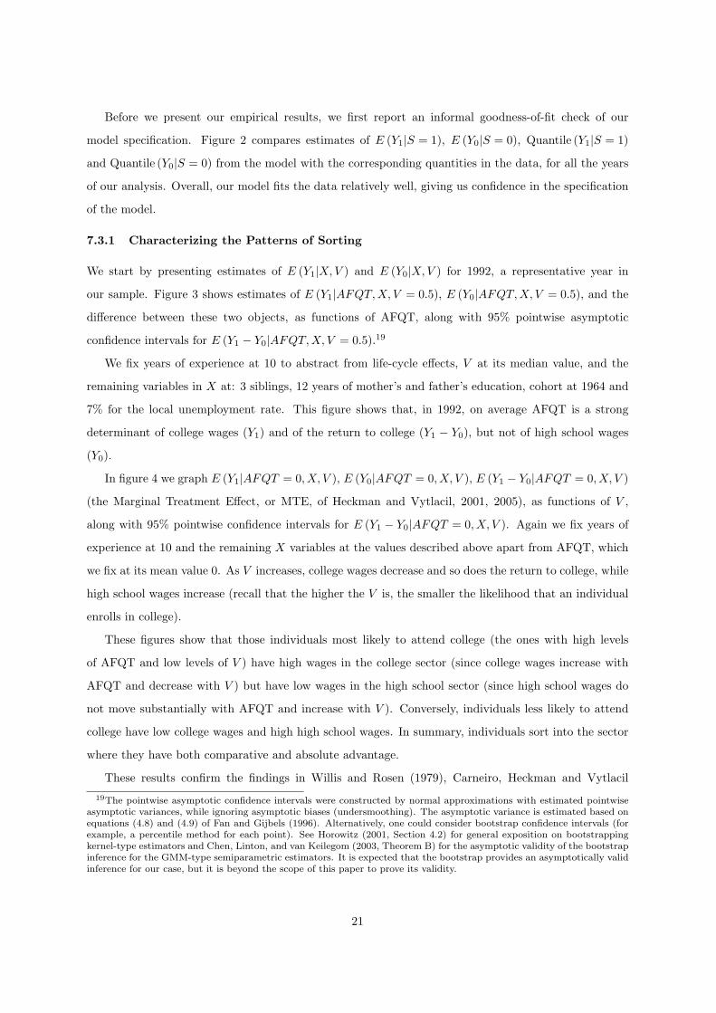
7.3.1 Characterizing the Patterns of Sorting

We start by presenting estimates of E (Y1|X,V ) and E (Y0|X, V ) for 1992, a representative year in

our sample. Figure 3 shows estimates of E (Y1|AFQT,X, V = 0.5), E (Y0|AFQT, X, V = 0.5), and the

difference between these two objects, as functions of AFQT, along with 95% pointwise asymptotic

confidence intervals for E (Y1 − Y0|AFQT, X, V = 0.5).19

We fix years of experience at 10 to abstract from life-cycle effects, V at its median value, and the

remaining variables in X at: 3 siblings, 12 years of mother’s and father’s education, cohort at 1964 and

7% for the local unemployment rate. This figure shows that, in 1992, on average AFQT is a strong

determinant of college wages (Y1) and of the return to college (Y1 − Y0), but not of high school wages

(Y0).

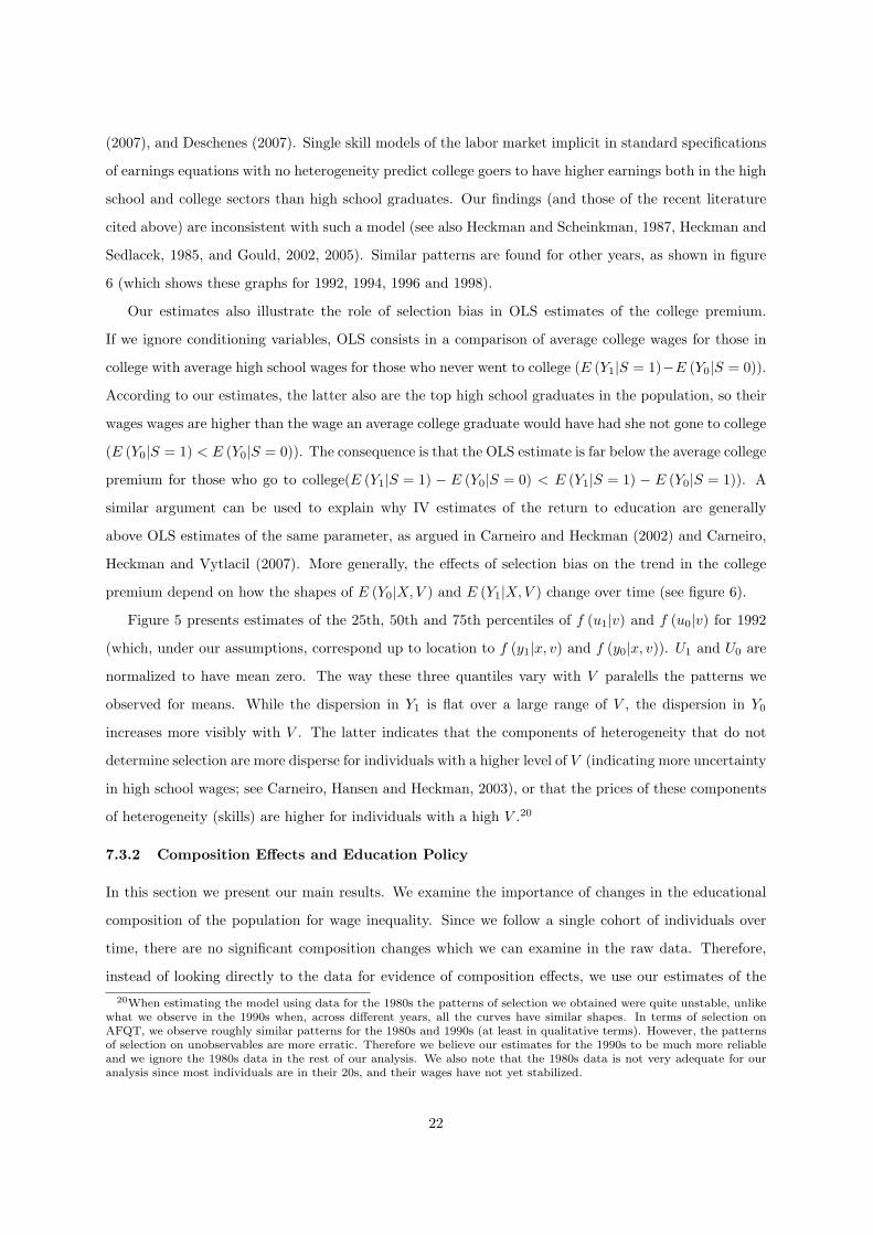
In figure 4 we graph E (Y1|AFQT = 0, X, V ), E (Y0|AFQT = 0, X, V ), E (Y1 − Y0|AFQT = 0, X, V )

(the Marginal Treatment Effect, or MTE, of Heckman and Vytlacil, 2001, 2005), as functions of V ,

along with 95% pointwise confidence intervals for E (Y1 − Y0|AFQT = 0, X, V ). Again we fix years of

experience at 10 and the remaining X variables at the values described above apart from AFQT, which

we fix at its mean value 0. As V increases, college wages decrease and so does the return to college, while

high school wages increase (recall that the higher the V is, the smaller the likelihood that an individual

enrolls in college).

These figures show that those individuals most likely to attend college (the ones with high levels

of AFQT and low levels of V ) have high wages in the college sector (since college wages increase with

AFQT and decrease with V ) but have low wages in the high school sector (since high school wages do

not move substantially with AFQT and increase with V ). Conversely, individuals less likely to attend

college have low college wages and high high school wages. In summary, individuals sort into the sector

where they have both comparative and absolute advantage.

These results confirm the findings in Willis and Rosen (1979), Carneiro, Heckman and Vytlacil

19The pointwise asymptotic confidence intervals were constructed by normal approximations with estimated pointwiseasymptotic variances, while ignoring asymptotic biases (undersmoothing). The asymptotic variance is estimated based onequations (4.8) and (4.9) of Fan and Gijbels (1996). Alternatively, one could consider bootstrap confidence intervals (forexample, a percentile method for each point). See Horowitz (2001, Section 4.2) for general exposition on bootstrappingkernel-type estimators and Chen, Linton, and van Keilegom (2003, Theorem B) for the asymptotic validity of the bootstrapinference for the GMM-type semiparametric estimators. It is expected that the bootstrap provides an asymptotically validinference for our case, but it is beyond the scope of this paper to prove its validity.

21

(2007), and Deschenes (2007). Single skill models of the labor market implicit in standard specifications

of earnings equations with no heterogeneity predict college goers to have higher earnings both in the high

school and college sectors than high school graduates. Our findings (and those of the recent literature

cited above) are inconsistent with such a model (see also Heckman and Scheinkman, 1987, Heckman and

Sedlacek, 1985, and Gould, 2002, 2005). Similar patterns are found for other years, as shown in figure

6 (which shows these graphs for 1992, 1994, 1996 and 1998).

Our estimates also illustrate the role of selection bias in OLS estimates of the college premium.

If we ignore conditioning variables, OLS consists in a comparison of average college wages for those in

college with average high school wages for those who never went to college (E (Y1|S = 1)−E (Y0|S = 0)).

According to our estimates, the latter also are the top high school graduates in the population, so their

wages wages are higher than the wage an average college graduate would have had she not gone to college

(E (Y0|S = 1) < E (Y0|S = 0)). The consequence is that the OLS estimate is far below the average college

premium for those who go to college(E (Y1|S = 1) − E (Y0|S = 0) < E (Y1|S = 1) − E (Y0|S = 1)). A

similar argument can be used to explain why IV estimates of the return to education are generally

above OLS estimates of the same parameter, as argued in Carneiro and Heckman (2002) and Carneiro,

Heckman and Vytlacil (2007). More generally, the effects of selection bias on the trend in the college

premium depend on how the shapes of E (Y0|X, V ) and E (Y1|X,V ) change over time (see figure 6).

Figure 5 presents estimates of the 25th, 50th and 75th percentiles of f (u1|v) and f (u0|v) for 1992

(which, under our assumptions, correspond up to location to f (y1|x, v) and f (y0|x, v)). U1 and U0 are

normalized to have mean zero. The way these three quantiles vary with V paralells the patterns we

observed for means. While the dispersion in Y1 is flat over a large range of V , the dispersion in Y0

increases more visibly with V . The latter indicates that the components of heterogeneity that do not

determine selection are more disperse for individuals with a higher level of V (indicating more uncertainty

in high school wages; see Carneiro, Hansen and Heckman, 2003), or that the prices of these components

of heterogeneity (skills) are higher for individuals with a high V .20

7.3.2 Composition Effects and Education Policy

In this section we present our main results. We examine the importance of changes in the educational

composition of the population for wage inequality. Since we follow a single cohort of individuals over

time, there are no significant composition changes which we can examine in the raw data. Therefore,

instead of looking directly to the data for evidence of composition effects, we use our estimates of the20When estimating the model using data for the 1980s the patterns of selection we obtained were quite unstable, unlike

what we observe in the 1990s when, across different years, all the curves have similar shapes. In terms of selection onAFQT, we observe roughly similar patterns for the 1980s and 1990s (at least in qualitative terms). However, the patternsof selection on unobservables are more erratic. Therefore we believe our estimates for the 1990s to be much more reliableand we ignore the 1980s data in the rest of our analysis. We also note that the 1980s data is not very adequate for ouranalysis since most individuals are in their 20s, and their wages have not yet stabilized.

22

selection and outcome equations to simulate what would happen to inequality if college enrollment rates

were different than the ones we observe, keeping prices fixed (partial equilibrium framework; see also

Ferreira and Leite, 2005).

The main difficulty of this exercise is to determine which individuals shift across schooling levels

when the college enrollment rate changes. This is why a model is needed. Even though our data is only

representative of a fixed set of cohorts working in the 1990s, our model can be useful for studying other

time periods. The restriction we face is that we can only simulate changes in composition for skill prices

fixed at their 1990s levels, and skill prices are probably higher in the 1990s than ever before. Therefore

composition effects will be larger when we evaluate them using 1990s prices than they would be if we

evaluated them instead using 1980s prices or 1970s prices. However, ultimately the choice of what base

prices we should use to evaluate composition effects depends on what question we would like to answer.

It is analogous to the choice of Laspeyres or Paasche price indices to analyze changes in prices over time.

We note also that, if skill prices are cohort specific (as suggested by Card and Lemieux, 2001), they may

be lower for younger cohorts than for older cohorts if the former have larger amounts of skill, which we

can probably presume to be the case.

The mechanics of the simulation are simple: first we change the intercept of the schooling equation

and we identify the distribution of (X,V ) for individuals who are induced to enroll in college; second we

generate the distribution of high school and college wages for this set of individuals; third, we compute

how their exit from the high school sector affects the high school wage distribution and how their entry

into the college sector affects the college wage distribution. The details of the simulation procedure

are presented in Appendix B.2. When conducting the simulations, our aim is to mimic the change in

college participation among working-age (25-65) white males that is observed between the 1980 and 1990

Censuses, which is an increase from 41% to 55%.

Table 3 (columns (1) and (2)) shows the result of an experiment where we increase the fraction of

individuals in college from 41% to 55% (which, according to the Census, is roughly the same change

that is observed from 1980 to 1990 for white males aged 25 to 65). The consequence is a decrease in

average college wages by 5%, and an increase in average high school wages by 7%. The reason is that

the marginal individuals induced to attend college are of below average college quality and they are also

of below average high school quality. As a result, the OLS estimate of the return to schooling decreases

from 54% to 42%.

We simulate much smaller changes in within group inequality and overall inequality as a result of

changes in composition. The ratio of the 90th to the 10th percentile of college wages increases from 1.29

to 1.31, an increase of 2%. In high school, the 90-10 percentile wage differential does not change. Finally,

our simulations show a very small decrease in the 90-10 differential in the overall wage distribution, from

23

1.30 to 1.29.

Our simulation shows that in the absence of composition effects the college premium in the 1980s

would have grown by 12 percentage points more than it did in the data. Even if we exaggerate the

magnitude of these effects by using 1990s prices, we conjecture that they would be still large if evaluated

at 1980s prices. Ignoring them would lead us to severely underpredict the increase in the college premium

in the 1980s. As a flip side, if we were to estimate the elasticity of substitution between college and high

school labor in this data, it would be overstated.

The consequences of our simulated changes in composition for within group inequality are smaller,

although they are still sizeable in the college sector. At first glance it is surprising to find large effects

of composition on between group inequality but small effects on within group and overall inequalities.

However, it is possible to reconcile these facts. This will happen if the amount of heterogeneity on which

individuals select does not explain a lot of the dispersion in wages. As emphasized in Carneiro, Hansen

and Heckman (2003) and Cunha, Heckman and Navarro (2005), even if the returns to schooling are very

heterogeneous across individuals, individuals only select on returns to the extent that this heterogeneity

is known at the time they make the schooling decision. In our data individuals do select into schooling

based on their returns. However, their ex-ante expectation of returns is quite imperfect, and it only

accounts for a small portion of the total dispersion in the returns to schooling.21 In such a context, it

is possible to have a large impact of changes in composition on average parameters such as the college

premium, but only a small effect on dispersion parameters, such as the 90-10 percentile ratio.

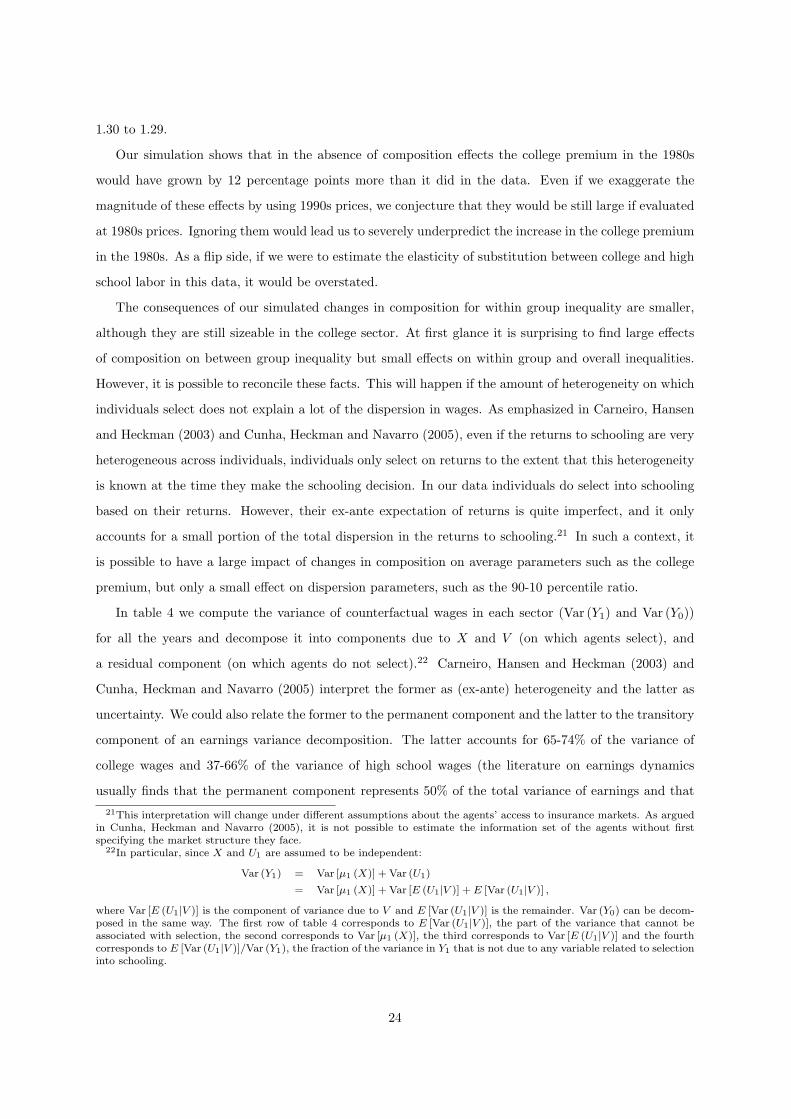
In table 4 we compute the variance of counterfactual wages in each sector (Var (Y1) and Var (Y0))

for all the years and decompose it into components due to X and V (on which agents select), and

a residual component (on which agents do not select).22 Carneiro, Hansen and Heckman (2003) and

Cunha, Heckman and Navarro (2005) interpret the former as (ex-ante) heterogeneity and the latter as

uncertainty. We could also relate the former to the permanent component and the latter to the transitory

component of an earnings variance decomposition. The latter accounts for 65-74% of the variance of

college wages and 37-66% of the variance of high school wages (the literature on earnings dynamics

usually finds that the permanent component represents 50% of the total variance of earnings and that21This interpretation will change under different assumptions about the agents’ access to insurance markets. As argued

in Cunha, Heckman and Navarro (2005), it is not possible to estimate the information set of the agents without firstspecifying the market structure they face.

22In particular, since X and U1 are assumed to be independent:

Var (Y1) = Var [µ1 (X)] + Var (U1)

= Var [µ1 (X)] + Var [E (U1|V )] + E [Var (U1|V )] ,

where Var [E (U1|V )] is the component of variance due to V and E [Var (U1|V )] is the remainder. Var (Y0) can be decom-posed in the same way. The first row of table 4 corresponds to E [Var (U1|V )], the part of the variance that cannot beassociated with selection, the second corresponds to Var [µ1 (X)], the third corresponds to Var [E (U1|V )] and the fourthcorresponds to E [Var (U1|V )]/Var (Y1), the fraction of the variance in Y1 that is not due to any variable related to selectioninto schooling.

24

this number is higher in college than high school; see, e.g., Meghir and Pistaferri, 2004).

7.3.3 The Importance of Selection Bias

The fact that individuals sort into different levels of schooling implies that selection bias affects both

within and between group inequality and their evolution over time. Selection bias is always defined

relatively to a specific parameter of interest. Here we illustrate the role of selection bias by comparing

inequality in the observed economy with inequality in a simulated counterfactual economy where indi-

viduals are randomly assigned to different schooling levels, as in Heckman and Sedlacek (1985, 1990).

Therefore, we assess the effect of selection bias on inequality parameters under random assignment. We

are able to approximate random assignment fairly well because we have close to full support on P ,

although, as mentioned above, this relies on the assumption of full independence between (X, Z) and

(U1, U0, V ).

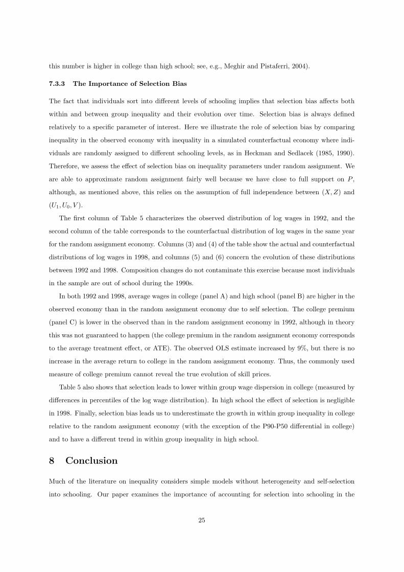
The first column of Table 5 characterizes the observed distribution of log wages in 1992, and the

second column of the table corresponds to the counterfactual distribution of log wages in the same year

for the random assignment economy. Columns (3) and (4) of the table show the actual and counterfactual

distributions of log wages in 1998, and columns (5) and (6) concern the evolution of these distributions

between 1992 and 1998. Composition changes do not contaminate this exercise because most individuals

in the sample are out of school during the 1990s.

In both 1992 and 1998, average wages in college (panel A) and high school (panel B) are higher in the

observed economy than in the random assignment economy due to self selection. The college premium

(panel C) is lower in the observed than in the random assignment economy in 1992, although in theory

this was not guaranteed to happen (the college premium in the random assignment economy corresponds

to the average treatment effect, or ATE). The observed OLS estimate increased by 9%, but there is no

increase in the average return to college in the random assignment economy. Thus, the commonly used

measure of college premium cannot reveal the true evolution of skill prices.

Table 5 also shows that selection leads to lower within group wage dispersion in college (measured by

differences in percentiles of the log wage distribution). In high school the effect of selection is negligible

in 1998. Finally, selection bias leads us to underestimate the growth in within group inequality in college

relative to the random assignment economy (with the exception of the P90-P50 differential in college)

and to have a different trend in within group inequality in high school.

8 Conclusion

Much of the literature on inequality considers simple models without heterogeneity and self-selection

into schooling. Our paper examines the importance of accounting for selection into schooling in the

25

empirical study of inequality. We estimate a semiparametric selection model with two levels of schooling

(high school and college) using four years of data (1992, 1994, 1996 and 1998) from the NLSY, and use

it for three different exercises. First, we use it to understand the main patterns of sorting of individuals

into different levels of schooling. We find that individuals sort into the level of schooling where they

have absolute and comparative advantage. Second, we use the model to simulate a change in college

enrollment and examine its effect on the wage structure. In our data increases in educational attainment

lead to reductions in between group inequality and increases in within group inequality in college. Third,

we use it to analyze the evolution of inequality and of its determinants in our sample during the 1990s,

purging our estimates of selection bias. We find that the trends in the commonly measured college wage

premium and within group inequality cannot reveal the trends of prices of skills.

We have also made two new contributions to the econometrics literature. First, we have extended

the method of local instrumental variables of Heckman and Vytlacil (1999, 2001, 2005) to identify the

distributions of potential outcomes. Second, we have developed a semiparametric method for estimating

the entire marginal distributions of potential outcomes.

Some of the effects we emphasize in this paper are also present in some analyses of larger samples.

Using the Census, Juhn, Kim and Vella (2005) find evidence of cohort quality effects systematically

related to the educational attainment of different cohorts, but argue these can only explain a small

fraction of recent fluctuations in the college premium. Carneiro and Lee (2007), using almost the same

data but an alternative approach, find larger effects. However, more work remains to be done.

Appendix

A Description of the Data

We restrict the NLSY sample to white males. We define four schooling categories: high school dropouts,

high school graduates, some college and college graduates. Because there are multiple useful reports of

schooling in the NLSY we construct the educational categories as follows: individuals without a high

school degree are high school dropouts; individuals with a high school degree but with less than 13 years

of schooling are high school graduates; those reporting 13 to 15 years of schooling and without a four

year college degree go into the some college group; finally, those reporting a four year college degree or

16 or more years of schooling are considered to be four year college graduates. GED recipients who never

attend college are included in the group of high school graduates. GED recipients that do not have a

high school degree, who have less than 12 years of schooling completed and who never reported college

attendance are excluded from the sample. The wage variables we use are deflated (to 1983) non-missing

hourly wages from 1990 to 2000. We use these to construct 5 year averages which we use in the analysis.

We delete all wage observations that are below 1 or above 100. Experience is actual work experience

in weeks accumulated from 1979 to the year of interest (annual weeks worked are imputed to be zero if

they are missing in any given year). The remaining variables that we include in the X and Z vectors are

26

number of siblings, father’s years of schooling, mother’s years of schooling, schooling corrected AFQT,

average tuition in four year colleges in the county of residence at age 17 deflated (to 1993), distance to

four-year colleges at age 14 and local unemployment rate in state of residence at age 17. The distance

variable, which is from Kling (2001), is an indicator variable whether a four-year college is in the county

of residence at age 14. The state unemployment rate data comes from the BLS website. However, from

the BLS website it is not possible to get state unemployment data for all states for all the 1970s (data

is available for all states from 1976 on, and it is available for 29 states for 1973, 1974 and 1975), and

therefore for some of the individuals we have to assign them the unemployment rate in the state of

residence in 1976 (which will correspond to age 19 for those born in 1957 and age 18 for those born

in 1958). Annual records on tuition, enrollment, and location of all public four year colleges in the

United States were constructed from the Department of Education’s annual Higher Education General

Information Survey and Integrated Postsecondary Education Data System “Institutional Characteristics’

surveys. By matching location with county of residence, we determined the presence of four-year colleges.

Tuition measures are taken as enrollment weighted averages of all public four-year colleges in a person’s

county of residence (if available) or at the state level if no college is available. County and state of

residence at 17 are not available for everyone in the NLSY, but only for the cohorts born in 1962, 1963

and 1964 (age 17 in 1979, 1980 and 1981). However, county and state of residence at age 14 is available

for most respondents. Therefore, we impute location at 17 to be equal to location at 14 for cohorts born

between 1957 and 1962 unless location at 14 is missing, in which case we use location in 1979 for the

imputation. For a description of the NLSY sample see BLS (2001). The NLSY79 has an oversample of

poor whites which we exclude from this analysis. We also exclude the military sample. To remove the

effect of schooling on AFQT we implement the same procedure as in Carneiro, Heckman and Vytlacil

(2007) (based on Hansen, Heckman and Mullen, 2004).

B More Details of Estimation Procedure

B.1 Obtaining Sample Analogs of (3.4)

Estimators of E[Yj ], E[Yj |S = 1], and E[Yj |S = 0] are obtained by

E[Yj ] = n−1n∑

i=1

∫ 1

0

E[Yj |X = Xi, V = v] dv,

E[Yj |S = 1] = n−1n∑

i=1

∫ 1

0

E[Yj |X = Xi, V = v]1− FP |X(v|Xi)

Pr(S = 1)dv,

and

E[Yj |S = 0] = n−1n∑

i=1

∫ 1

0

E[Yj |X = x, V = v]FP |X(v|Xi)

Pr(S = 0)dv,

(B.1)

where E[Yj |X = x, V = v] = µj(x, βj) + E[Uj |V = v] is defined in section 4.2, FP |X(v|x) is a non-

parametric estimator of FP |X(v|x), and Pr(S = j) is the sample proportion of S = j for j = 0, 1. The

integration with respect to v can be evaluated numerically.

27

B.2 Simulating Wage distributions of Different Compositions of EducationGroups

This subsection describes how we carry out simulations whose results are shown in table 3. Suppose

there is a policy that shifts the distribution of P in the population from FP |X (p|x) to F ∗P |X (p|x), but

has no effect on f (y0|x, v) nor f (y1|x, v). In view of (3.4), the post-policy distributions of college and

high school wages are

f(y1|S = 1) =∫ ∫ 1

0

f(y1|x, v)1− F ∗P |X(v|x)

Pr∗(S = 1)fX(x) dv dx,

and

f(y0|S = 0) =∫ ∫ 1

0

f(y0|x, v)F ∗P |X(v|x)

Pr∗(S = 0)fX(x) dv dx.

(B.2)

Thus, in order to simulate wage distributions of different compositions of education groups, we need to

compute only F ∗P |X (p|x) and Pr∗(S = 1). Recall that in our empirical work, P = L(µS(Z)), where

L is the CDF of the logistic distribution. We simulate changes in college enrollment rates simply by

varying the intercept of µS . Then F ∗P |X (p|x) can be estimated by a nonparametric kernel regression of

1L(µS(Z) + c∗) ≤ p on X with an estimated choice index µ and Pr∗(S = 1) can be estimated by a

sample average of L(µS(Z) + c∗), where we choose the values of c∗ to match college enrollment rates in

1980 and 1990. Finally the results shown in table 3 can be obtained by sample analogs of (B.2).

C Mathematical Proofs

Proof of Theorem 2. Given the partially linear additive structure in the modelling of P , this lemma is

a direct consequence of Theorem 7 of Newey (1997).

Proof of Theorem 3. This can be proved using general results for two-step semiparametric estimators.

In particular, we verify regularity conditions of Ichimura and Lee (2006, hereafter IL) and apply their

general theorem to our case. We consider only the case that j = 1. The other case is very similar. Now

we view the estimator β1 as an M-estimator with

m [(y, s, x, z), b, f(·)] =12s [y − f1(f3(z))− x− f2(f3(z))′b]2 ,

where f = (f1, f2, f3) are the nonparametric components of the model. In particular, the true function

f0 = (f10, f20, f30) satisfies f10(·) = E[Y |P = ·], f20(·) = E[X|P = ·], and f30(·) = E[S|Z = ·].First, we check their regularity conditions. Assumption 3.1(a) of IL is not needed in our case because

we have an estimator that minimizes a convex objective function. Assumptions 3.1(b) is guaranteed

by the assumption that Ωj is positive definite (see Section 4 of Robinson, 1988). The consistency of

the estimator can be easily obtained in view of Assumption 7, so that Assumption 3.1(c) is satisfied.

Assumptions 3.2 and 3.3 of IL are trivially satisfied given the form of the objective function m. In view

of Theorem 2, Assumption 8 implies that

maxi:1≤i≤n

|P (Zi)− P (Zi)| = op

(n−1/4

).

Then using this and Assumption 7, Assumption 3.4 of IL is easily verified. Given the form of m, it is

trivial to verify Assumption 3.5 of IL (see, Proposition 3.1 of IL and discussions on Examples 2.2 and 2.3

28

of IL). Assumption 3.6 of IL is a key assumption that characterizes the effect of the first stage estimation

of P . Using the notation that is same as in IL, it is straightforward to calculate

Df1m∗(b, f0(·))[h1(·)] = −E [S (Y − E[Y |P ])− (µ1(X)− E[µ1(X)|P ])′bh1(·)] ,

Df2m∗(b, f0(·))[h2(·)] = E [S (Y − E[Y |P ])− (µ1(X)− E[µ1(X)|P ])′bh2(·)′b] ,

Df3m∗(b, f0(·))[h3(·)] = E

[S (Y − E[Y |P ])− (µ1(X)− E[µ1(X)|P ])′b

×−∂f10(p)/∂p

∣∣p=P

+ ∂f20(p)/∂p′∣∣p=P

b

h3(·)].

Then it easy to see that

∂

∂bDf1m

∗(b, f0(·))[h1(·)]∣∣b=β1

= 0,

∂

∂bDf2m

∗(b, f0(·))[h2(·)]∣∣b=β1

= 0,

∂

∂bDf3m

∗(b, f0(·))[h3(·)]∣∣b=β1

= E[S(µ1(X)− E[µ1(X)|P ])∂λ1(p)/∂p

∣∣p=P

h3(·)].

Thus, only the third term above affects the asymptotic distribution. Its limiting behavior evaluated at

P −P is easy to describe, because it is a linear functional of P −P . For example, see Section 4 of Newey

(1997). Assumption 7 of Newey (1997) is satisfied with ν(z) that is defined above (see Assumption 9).

Then the desired result follows from Theorem 3.3 of IL with the restriction that n1/2κ−rϕ → 0.

Proof of Theorem 4. Define U =[U11, . . . , U1n

]′and Wh = diag

S1Kh(P1 − v), . . . , SnKh(Pn − v)

]′,

where Kh(·) = h−1K(·/h). In addition, define

XL =

1 (P1 − v)...

...1 (Pn − v)

and XQ =

1 (P1 − v) (P1 − v)2...

......

1 (Pn − v) (Pn − v)2

.

Then using this notation, it follows from (4.4) that

E[U1|V = v] = v × e′2(X′

QWhn2XQ

)−1 (X′

QWhn2U)

+ e′1(X′

LWhn1XL

)−1 (X′

LWhn1U)

,(C.1)

where e1 = (1, 0)′ and e2 = (0, 1, 0)′.

Let U = [U11, . . . , U1n]′ and µ1(X) = [µ1(X1), . . . , µ1(Xn)]. Since U1i = U1i−µ1(Xi)′(β1 − β1

), we

have

E[U1|V = v] = Tn(v)−Rn(v)(β1 − β1

),(C.2)

where

Tn(v) = v × e′2(X′

QWhn2XQ

)−1 (X′

QWhn2U)

+ e′1(X′

LWhn1XL

)−1 (X′

LWhn1U)

Rn(v) = v × e′2(X′

QWhn2XQ

)−1 (X′

QWhn2µ1(X))

+ e′1(X′

LWhn1XL

)−1 (X′

LWhn1µ1(X))

.

Then since Rn(v) = Op(1),

E[U1|V = v] = Tn(v) + Op

(n−1/2

),(C.3)

which implies that the error from estimating β1 is asymptotically negligible.

29

To analyze Tn(v), define

U∗ = (E[U1|P = P1, S = 1], . . . , E[U1|P = Pn, S = 1])′

and

XL =

1 (P1 − v)...

...1 (Pn − v)

and XQ =

1 (P1 − v) (P1 − v)2...

......

1 (Pn − v) (Pn − v)2

.

It follows from Assumptions 11 and 12 that

maxi

∣∣∣Kh(Pi − v)−Kh(Pi − v)∣∣∣ = op(1),(C.4)

which implies that∥∥∥Whn1 −Whn1

∥∥∥ = op(1). By Taylor series expansion,

E[U1|P = Pi, S = 1] = E[U1|P = v, S = 1] +∂E[U1|P = v, S = 1]

∂p(Pi − v)

+12

∂2E[U1|P = v, S = 1]∂p2

(Pi − v)2 +13!

∂3E[U1|P = v, S = 1]∂p3

(Pi − v)3 + Rp(v),

where Rp(v) is a Taylor remainder term. Further, expand the equation above as

E[U1|P = Pi, S = 1] = E[U1|P = v, S = 1]

+∂E[U1|P = v, S = 1]

∂p(Pi − v)− ∂E[U1|P = v, S = 1]

∂p(Pi − Pi)

+12

∂2E[U1|P = v, S = 1]∂p2

(Pi − v)2

+13!

∂3E[U1|P = v, S = 1]∂p3

(Pi − v)3 + Rp(v).

(C.5)

Using (C.4) and (C.5), we have

e′1(X′

LWhn1XL

)−1 (X′

LWhn1U)− E[U1|P = v, S = 1]

= e′1(X′

LWhn1XL

)−1 (X′

LWhn1 [U−U∗])

+ Op

(max

i:1≤i≤n|Pi − Pi|+ h2

n1

)

= e′1 (X′LWhn1XL)−1 (X′

LWhn1 [U−U∗]) [1 + op(1)] + Op

(max

i:1≤i≤n|Pi − Pi|+ h2

n1

)

= Op

((nhn1)−1/2 + max

i:1≤i≤n|Pi − Pi|+ h2

n1

).

Similar arguments also give

e′2(X′

QWhn2XQ

)−1 (X′

QWhn2U)− ∂E[U1|P = v, S = 1]

∂p

= e′2(X′

QWhn2XQ

)−1 (X′

QWhn2 [U−U∗])

+ Op

(max

i:1≤i≤n|Pi − Pi|+ h2

n2

)

= e′2(X′

QWhn2XQ

)−1 (X′

QWhn2 [U−U∗])[1 + op(1)] + Op

(max

i:1≤i≤n|Pi − Pi|+ h2

n2

)

= Op

((nh3

n2)−1/2 + max

i:1≤i≤n|Pi − Pi|+ h2

n2

).

Then the theorem follows from standard results on local polynomial regression (for example, see Chapter

3 of Fan and Gijbels, 1996).

30

References

Abadie, A. (2002), “Bootstrap Tests for Distributional Treatment Effects in Instrumental VariableModels,” Journal of the American Statistical Association, 97: 284-292.

Abadie, A. (2003), Semiparametric instrumental variable estimation of treatment response models,Journal of Econometrics, 113:2, 231-263.

Abadie, A., J. D. Angrist, and G. W. Imbens (2002), “Instrumental Variables Estimates of the Effectof Subsidized Training on the Quantiles of Trainee Earnings,” Econometrica, 70: 91-117.

Acemoglu, D. (2002), Technical Change, Inequality and the Labor Market, Journal of Economic Lit-erature, 40: 7-72.

Autor, D., L. Katz and M. Kearney (2007), “Trends in U.S. Wage Inequality: Re-Assessing the Revi-sionists”, Review of Economics and Statistics, forthcoming .

Aakvik, A., Heckman, J. and E. Vytlacil (2005), Estimating treatment effects for discrete outcomeswhen responses to treatment vary: an application to Norwegian vocational rehabilitation programs,Journal of Econometrics, 125:1-2, 15-51.

Cameron, S. and C. Taber (2004), “Estimation of Educational Borrowing Constraints Using Returnsto Schooling”, Journal of Political Economy, part 1, 112(1): 132-82.

Card, D. (1995), “Using Geographic Variation in College Proximity to Estimate the Return to School-ing ”, Aspects of Labour Economics: Essays in Honour of John Vanderkamp, edited by LouisChristofides, E. Kenneth Grant and Robert Swindinsky. University of Toronto Press.

Card, D. (1999), “The Causal Effect of Education on Earnings,” Orley Ashenfelter and David Card,(editors), Vol. 3A, Handbook of Labor Economics, Amsterdam: North-Holland.

Card, D. (2001), “Estimating the Return to Schooling: Progress on Some Persistent EconometricProblems,” Econometrica, 69(5): 1127-60.

Card, D. and T. Lemieux (2001), “Can Falling Supply Explain the Rising Return to College For YoungerMen? A Cohort Based Analysis,” Quarterly Journal of Economics 116: 705-46.

Carneiro, P. and J. Heckman (2002), “The Evidence on Credit Constraints in Post-secondary School-ing,” Economic Journal 112(482): 705-34.

Carneiro, P., K. Hansen and J. Heckman (2003), “Estimating Distributions of Counterfactuals withan Application to the Returns to Schooling and Measurement of the Effects of Uncertainty onSchooling Choice,” International Economic Review, 44(2): 361-422.

Carneiro, P., J. Heckman and E. Vytlacil (2007), “Understanding what Instrumental Variables estimate:estimating average and marginal returns to schooling”, working paper, The University of Chicago.

Carneiro, P. and S. Lee (2007), “Trends in Quality-Adjusted Skill Premia in the United States, 1960-2000”, working paper, University College London.

Chay, K. Y. and D. S. Lee (2000), “Changes in Relative Wages in the 1980s: Returns to Observed andUnobserved Skills and Black-White Wage Differentials,” Journal of Econometrics, 99: 1-38.

Chen, S. H. and S. Khan (2007), Estimating the Causal Effects of Education on Wage Inequality UsingIV Methods and Sample Selection Models, working paper, SUNY at Albany.

Chen, X, O. Linton, and I. van Keilegom (2003), Estimation of semiparametric models when thecriterion function is not smooth, Econometrica, 71:5, 1591-1608.

Chernozhukov, V. and C. Hansen (2005), “An IV model of Quantile Treatment Effects,” Econometrica,73(1): 245-61.

Chernozhukov, V. and C. Hansen (2006): Instrumental quantile regression inference for structural andtreatment effect models, Journal of Econometrics, 132, 491-525.

31

Chernozhukov, V., G. W. Imbens, and W. K. Newey (2007): Instrumental variable estimation ofnonseparable models, Journal of Econometrics, 139, 4-14.

Chesher, A. D. (2003), “Identification in Nonseparable Models,” Econometrica, 71: 1405-1441.

Cunha, F., J. Heckman and S. Navarro (2005), “Separating uncertainty from heterogeneity in life cycleearnings”, Oxford Economic Papers, 57: 191 - 261.

Currie, J. and E. Moretti (2003), Mother’s Education and the Intergenerational Transimission of HumanCapital: Evidence from College Openings, Quartely Journal of Economics, 118:4.

Das, M., W. K. Newey and F. Vella (2003), “Nonparametric Estimation of Sample Selection Models,”Review of Economics Studies, 70: 33-58.

Deschenes, O. (2007), “Estimating the Impact of Family Background on the Returns to Education”,Journal of Business and Economic Statistics, 25(3): 265-277.

Deschenes, O. (2006), “Unobserved Ability, Comparative Advantage, and the Rising Return to Collegein the United States, 1979-2002”, working paper, University of California Santa Barbara.

Fan, J. and I. Gijbels (1996), Local Polynomial Modelling and Its Applications (London: Chapman &Hall).

Fan, J., Q. Yao, and H. Tong (1996), “Estimation of Conditional Densities and Sensitivity Measures inNonlinear Dynamical Systems,” Biometrika: 83:189-206.

Ferreira, F. and P. Leite (2005), Educational Expansion and Income Distribution: a Micro-Simulationfor Ceara, in A. Shorrocks and R. Hoeven, Growth, Inequality and Poverty: Prospects for Pro-poorEconomic Development, Oxford University Press.

Galor, O. and O. Moav (2001), “Ability-Biased Technological Transition, Wage Inequality, and Eco-nomic Growth”, The Quarterly Journal of Economics, 115(2), 469-497.

Gosling, A., S. Machin, and C. Meghir (2000), “The Changing Distribution of Male Wages in the U.K.,”Review of Economic Studies, 67(4): 635-66.

Gould, E. D. (2002), “Rising Wage Inequality, Comparative Advantage, and the Growing Importanceof General Skills in the United States,” Journal of Labor Economics, 20(1): 105-47.

Gould, E. D. (2005), “Inequality and Ability”, Labour Economics, 12, 169-189.

Hansen, K., K. Mullen and J. Heckman (2004), “The Effect of Schooling and Ability on AchievementTest Scores,” Journal of Econometrics. 121(1-2): 39-98.

Heckman, J., H. Ichimura, J. Smith, and P. Todd (1998), “Characterizing Selection Bias Using Exper-imental Data,” Econometrica, 66, 1017-1098.

Heckman J. and S. Navarro (2007), “Dynamic discrete choice and dynamic treatment effects”, Journalof Econometrics, Volume 136, 341-396.

Heckman, J. and J. Scheinkman (1987), “The Importance of Bundling in a Gorman-Lancaster Modelof Earnings”, Review of Economic Studies, Vol. 54, No. 2., pp. 243-255.

Heckman, J. and G. Sedlacek (1985), “Heterogeneity, Aggregation and Market Wage Functions: AnEmpirical Model of Self-Selection in the Labor Market”, Journal of Political Economy, Vol. 93,No. 6., pp. 1077-1125.

Heckman, J. and G. Sedlacek (1990), Self-Selection and the Distribution of Hourly Wages, Journal ofLabor Economics, Vol. 8, No. 1, Part 2, pp. S329-S363.

Heckman, J., S. Urzua, and E. Vytlacil (2006), Understanding Instrumental Variables in Models withEssential Heterogeneity, Review of Economics and Statistics August, 88:3, 389-432.

Heckman, J. and E. Vytlacil (1999), Local Instrumental Variable and Latent Variable Models forIdentifying and Bounding Treatment Effects, Proceedings of the National Academy of Sciences, 96,4730-4734.

32

Heckman, J. and E. Vytlacil (2001), “Local Instrumental Variables,” in C. Hsiao, K. Morimune, and J.Powells, (eds.), Nonlinear Statistical Modeling: Proceedings of the Thirteenth International Sympo-sium in Economic Theory and Econometrics: Essays in Honor of Takeshi Amemiya, (Cambridge:Cambridge University Press, 2000), 1-46.

Heckman, J. and E. Vytlacil (2005), “Structural Equations, Treatment, Effects and Econometric PolicyEvaluation,” Econometrica, 73(3):669-738.

Horowitz, J. L. (2001), The Bootstrap, Edited by: J.J. Heckman and E. Leamer, Handbook of Econo-metrics Volume 5 3159-3228.

Horowitz, J. L. and S. Lee (2007): Nonparametric instrumental variables estimation of a quantileregression model, Econometrica, 75: 1191-1208.

Ichimura, H., and C. Taber (2000), Direct Estimation of Policy Impacts, Northwestern University,unpublished manuscript.

Ichimura, H. and S. Lee (2006): Characterization of the asymptotic distribution of semiparametricM-estimators, Cemmap Working Papers, CWP15/06, available at:http://cemmap.ifs.org.uk.

Imbens, G. and J. Angrist (1994), “Identification and Estimation of Local Average Treatment Effects,”Econometrica, 62(2):467-475.

Imbens, G. and W. Newey (2003), “Identification and Estimation of Triangular Simultaneous EquationsModels Without Additivity”, working paper, MIT.

Imbens, G. and D. Rubin (1997), “Estimating Outcome Distributions for Compliers in InstrumentalVariable Models,” Review of Economics Studies, 64: 555-574.

Juhn, C., D. -L. Kim, and F. Vella (2005), “The Expansion of College Education in the United States:Is There Evidence of Declining Cohort Quality?,” Economic Inquiry, 43(2): 303-15.

Juhn, C., K. Murphy and B. Pierce (1993), “Wage Inequality and the Rise in Returns to Skill”, Journalof Political Economy, 101(3):410-442.

Kane, T. and C. Rouse (1995), “Labor-Market Returns to Two- and Four-Year College”, AmericanEconomic Review, 85(3):600-614.

Katz, L. and D. Autor (1999), “Changes in the Wage Structure and Earnings Inequality”, in O. Ashen-felter and D. Card, eds, Handbook of Labor Economics, volume 3, North-Holland.

Katz, L. and K. Murphy (1992), “Changes in Relative Wages, 1963-1987: Supply and Demand Factors”,Quarterly Journal of Economics, Vol. 107, No. 1. (Feb., 1992), pp. 35-78.

Kling, J. (2001), “Interpreting Instrumental Variables Estimates of the Returns to Schooling”, Journalof Business and Economic Statistics, 19(3), 358-364.

Lee, S. (2007): Endogeneity in quantile regression models: A control function approach, Journal ofEconometrics, 141, 1131-1158.

Ma, L. and R. Koenker (2006): Quantile regression methods for recursive structural equation models,Journal of Econometrics, 134, 471-506.

R. A. Moffitt (2007): Estimating Marginal Returns to Higher Education in the UK, NBER WorkingPaper No. 13534.

Meghir, C. and L. Pistaferri (2004), “Income Variance Dynamics and Heterogeneity”, Econometrica,72(1): 1-32.

W. K. Newey (1997): Convergence rates and asymptotic normality for series estimators, Journal ofEconometrics, 79, 147-168.

Robinson, P. M. (1988), “Root- N-Consistent Semiparametric Regression,” Econometrica, 56(4): 931-54.

33

Silverman, B. W. (1986), Density Estimation for Statistics and Data Analysis, London: Chapman andHall.

Taber, C. R. (2001), “The Rising College Premium in the Eighties: Return to College or Return toUnobserved Ability?,” Review of Economic Studies, 68(3): 665-91.

Vytlacil, E. (2002): Independence, Monotonicity, and Latent Index Models: An Equivalence ResultEconometrica, 70, 331-341.

Vytlacil, E. and N. Yildiz (2007), “Dummy Endogenous Variables in Weakly Separable Models,” Econo-metrica, 75(3): 757-779.

Willis, R. and S. Rosen (1979), “Education and Self-Selection,” Journal of Political Economy, 87(5):Pt2:S7-36.

34

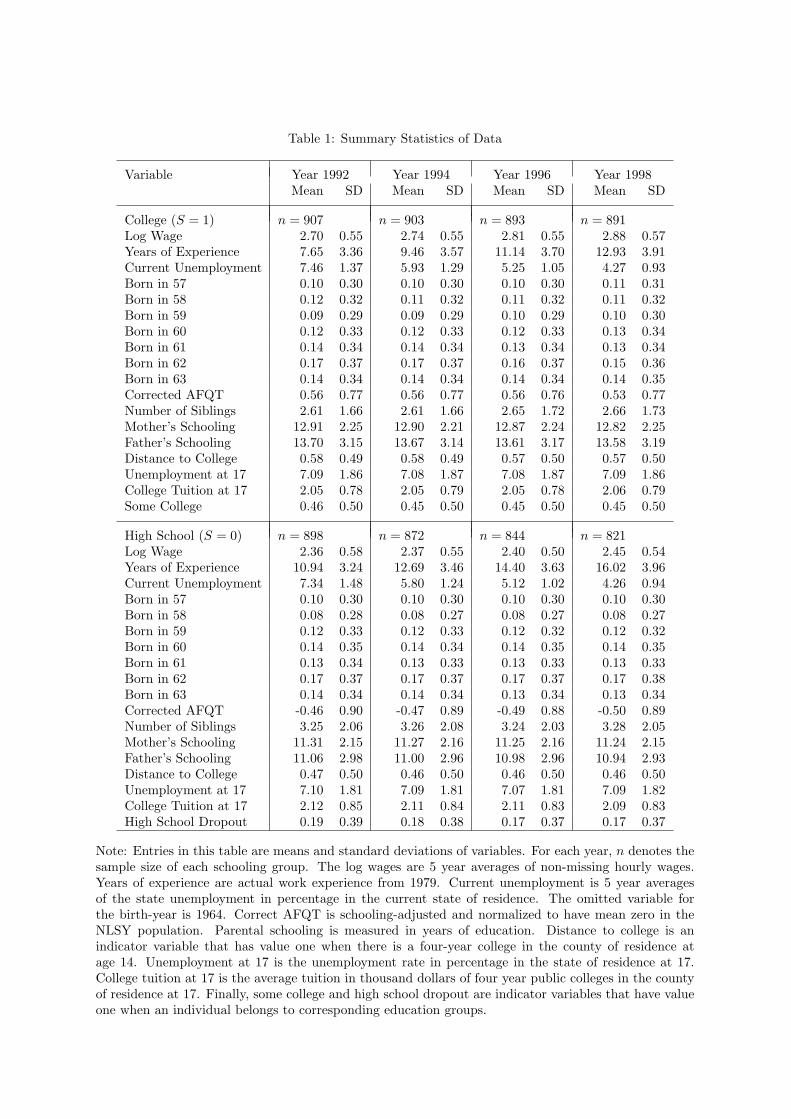
Table 1: Summary Statistics of Data

Variable Year 1992 Year 1994 Year 1996 Year 1998Mean SD Mean SD Mean SD Mean SD

College (S = 1) n = 907 n = 903 n = 893 n = 891Log Wage 2.70 0.55 2.74 0.55 2.81 0.55 2.88 0.57Years of Experience 7.65 3.36 9.46 3.57 11.14 3.70 12.93 3.91Current Unemployment 7.46 1.37 5.93 1.29 5.25 1.05 4.27 0.93Born in 57 0.10 0.30 0.10 0.30 0.10 0.30 0.11 0.31Born in 58 0.12 0.32 0.11 0.32 0.11 0.32 0.11 0.32Born in 59 0.09 0.29 0.09 0.29 0.10 0.29 0.10 0.30Born in 60 0.12 0.33 0.12 0.33 0.12 0.33 0.13 0.34Born in 61 0.14 0.34 0.14 0.34 0.13 0.34 0.13 0.34Born in 62 0.17 0.37 0.17 0.37 0.16 0.37 0.15 0.36Born in 63 0.14 0.34 0.14 0.34 0.14 0.34 0.14 0.35Corrected AFQT 0.56 0.77 0.56 0.77 0.56 0.76 0.53 0.77Number of Siblings 2.61 1.66 2.61 1.66 2.65 1.72 2.66 1.73Mother’s Schooling 12.91 2.25 12.90 2.21 12.87 2.24 12.82 2.25Father’s Schooling 13.70 3.15 13.67 3.14 13.61 3.17 13.58 3.19Distance to College 0.58 0.49 0.58 0.49 0.57 0.50 0.57 0.50Unemployment at 17 7.09 1.86 7.08 1.87 7.08 1.87 7.09 1.86College Tuition at 17 2.05 0.78 2.05 0.79 2.05 0.78 2.06 0.79Some College 0.46 0.50 0.45 0.50 0.45 0.50 0.45 0.50

High School (S = 0) n = 898 n = 872 n = 844 n = 821Log Wage 2.36 0.58 2.37 0.55 2.40 0.50 2.45 0.54Years of Experience 10.94 3.24 12.69 3.46 14.40 3.63 16.02 3.96Current Unemployment 7.34 1.48 5.80 1.24 5.12 1.02 4.26 0.94Born in 57 0.10 0.30 0.10 0.30 0.10 0.30 0.10 0.30Born in 58 0.08 0.28 0.08 0.27 0.08 0.27 0.08 0.27Born in 59 0.12 0.33 0.12 0.33 0.12 0.32 0.12 0.32Born in 60 0.14 0.35 0.14 0.34 0.14 0.35 0.14 0.35Born in 61 0.13 0.34 0.13 0.33 0.13 0.33 0.13 0.33Born in 62 0.17 0.37 0.17 0.37 0.17 0.37 0.17 0.38Born in 63 0.14 0.34 0.14 0.34 0.13 0.34 0.13 0.34Corrected AFQT -0.46 0.90 -0.47 0.89 -0.49 0.88 -0.50 0.89Number of Siblings 3.25 2.06 3.26 2.08 3.24 2.03 3.28 2.05Mother’s Schooling 11.31 2.15 11.27 2.16 11.25 2.16 11.24 2.15Father’s Schooling 11.06 2.98 11.00 2.96 10.98 2.96 10.94 2.93Distance to College 0.47 0.50 0.46 0.50 0.46 0.50 0.46 0.50Unemployment at 17 7.10 1.81 7.09 1.81 7.07 1.81 7.09 1.82College Tuition at 17 2.12 0.85 2.11 0.84 2.11 0.83 2.09 0.83High School Dropout 0.19 0.39 0.18 0.38 0.17 0.37 0.17 0.37

Note: Entries in this table are means and standard deviations of variables. For each year, n denotes thesample size of each schooling group. The log wages are 5 year averages of non-missing hourly wages.Years of experience are actual work experience from 1979. Current unemployment is 5 year averagesof the state unemployment in percentage in the current state of residence. The omitted variable forthe birth-year is 1964. Correct AFQT is schooling-adjusted and normalized to have mean zero in theNLSY population. Parental schooling is measured in years of education. Distance to college is anindicator variable that has value one when there is a four-year college in the county of residence atage 14. Unemployment at 17 is the unemployment rate in percentage in the state of residence at 17.College tuition at 17 is the average tuition in thousand dollars of four year public colleges in the countyof residence at 17. Finally, some college and high school dropout are indicator variables that have valueone when an individual belongs to corresponding education groups.

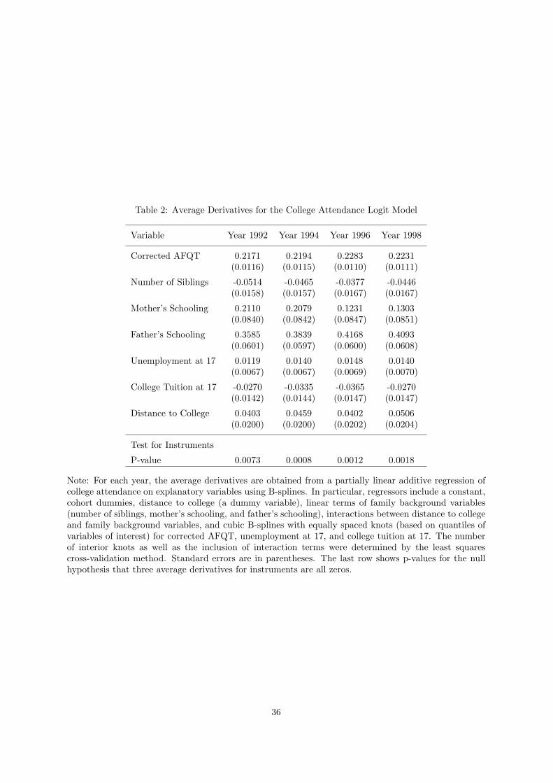
Table 2: Average Derivatives for the College Attendance Logit Model

Variable Year 1992 Year 1994 Year 1996 Year 1998

Corrected AFQT 0.2171 0.2194 0.2283 0.2231(0.0116) (0.0115) (0.0110) (0.0111)

Number of Siblings -0.0514 -0.0465 -0.0377 -0.0446(0.0158) (0.0157) (0.0167) (0.0167)

Mother’s Schooling 0.2110 0.2079 0.1231 0.1303(0.0840) (0.0842) (0.0847) (0.0851)

Father’s Schooling 0.3585 0.3839 0.4168 0.4093(0.0601) (0.0597) (0.0600) (0.0608)

Unemployment at 17 0.0119 0.0140 0.0148 0.0140(0.0067) (0.0067) (0.0069) (0.0070)

College Tuition at 17 -0.0270 -0.0335 -0.0365 -0.0270(0.0142) (0.0144) (0.0147) (0.0147)

Distance to College 0.0403 0.0459 0.0402 0.0506(0.0200) (0.0200) (0.0202) (0.0204)

Test for Instruments

P-value 0.0073 0.0008 0.0012 0.0018

Note: For each year, the average derivatives are obtained from a partially linear additive regression ofcollege attendance on explanatory variables using B-splines. In particular, regressors include a constant,cohort dummies, distance to college (a dummy variable), linear terms of family background variables(number of siblings, mother’s schooling, and father’s schooling), interactions between distance to collegeand family background variables, and cubic B-splines with equally spaced knots (based on quantiles ofvariables of interest) for corrected AFQT, unemployment at 17, and college tuition at 17. The numberof interior knots as well as the inclusion of interaction terms were determined by the least squarescross-validation method. Standard errors are in parentheses. The last row shows p-values for the nullhypothesis that three average derivatives for instruments are all zeros.

36

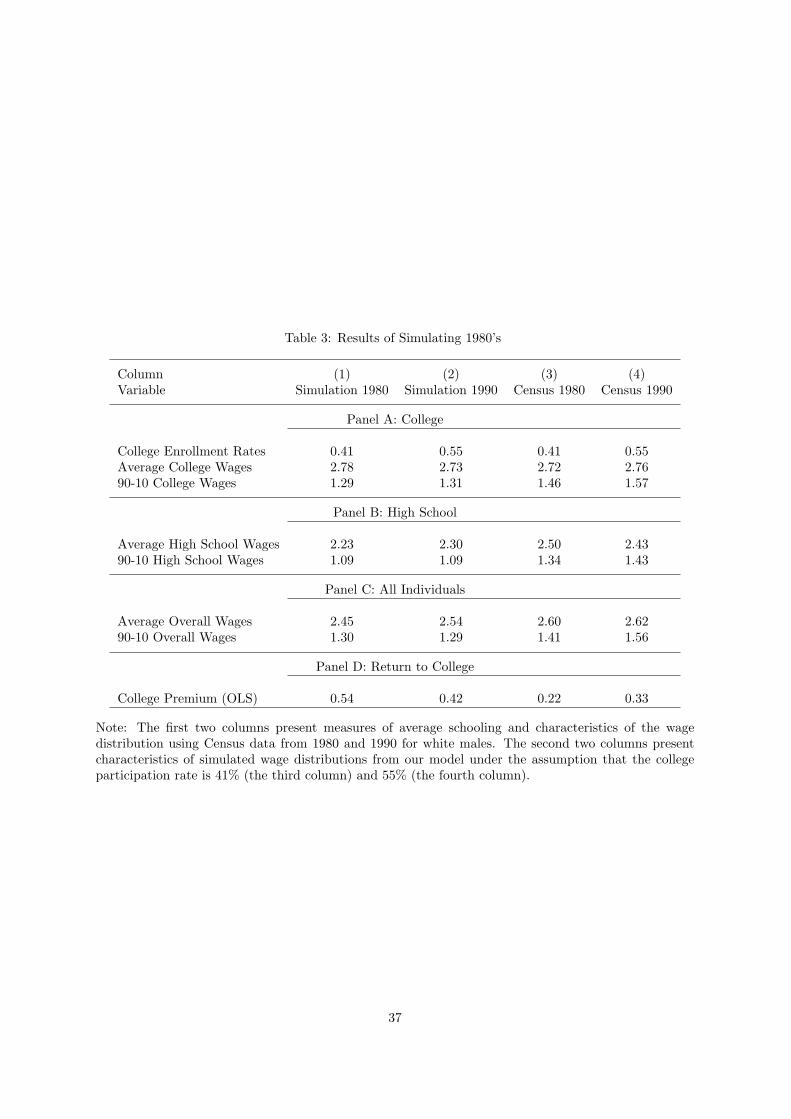
Table 3: Results of Simulating 1980’s

Column (1) (2) (3) (4)Variable Simulation 1980 Simulation 1990 Census 1980 Census 1990

Panel A: College

College Enrollment Rates 0.41 0.55 0.41 0.55Average College Wages 2.78 2.73 2.72 2.7690-10 College Wages 1.29 1.31 1.46 1.57

Panel B: High School

Average High School Wages 2.23 2.30 2.50 2.4390-10 High School Wages 1.09 1.09 1.34 1.43

Panel C: All Individuals

Average Overall Wages 2.45 2.54 2.60 2.6290-10 Overall Wages 1.30 1.29 1.41 1.56

Panel D: Return to College

College Premium (OLS) 0.54 0.42 0.22 0.33

Note: The first two columns present measures of average schooling and characteristics of the wagedistribution using Census data from 1980 and 1990 for white males. The second two columns presentcharacteristics of simulated wage distributions from our model under the assumption that the collegeparticipation rate is 41% (the third column) and 55% (the fourth column).

37

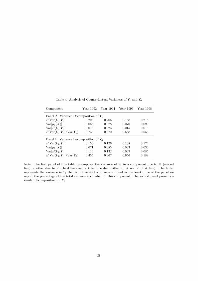
Table 4: Analysis of Counterfactual Variances of Y1 and Y0

Component Year 1992 Year 1994 Year 1996 Year 1998

Panel A: Variance Decomposition of Y1

E[Var(U1|V )] 0.223 0.206 0.188 0.218Var[µ1(X)] 0.068 0.078 0.070 0.099Var[E(U1|V )] 0.013 0.023 0.015 0.015E[Var(U1|V )]/Var(Y1) 0.736 0.670 0.688 0.656

Panel B: Variance Decomposition of Y0

E[Var(U0|V )] 0.156 0.126 0.138 0.174Var[µ0(X)] 0.071 0.085 0.033 0.036Var[E(U0|V )] 0.116 0.132 0.039 0.085E[Var(U0|V )]/Var(Y0) 0.455 0.367 0.656 0.589

Note: The first panel of this table decomposes the variance of Y1 in a component due to X (secondline), another due to V (third line) and a third one due neither to X nor V (first line). The latterrepresents the variance in Y1 that is not related with selection and in the fourth line of the panel wereport the percentage of the total variance accounted for this component. The second panel presents asimilar decomposition for Y0.

38

Table 5: The Impact of Self-Selection on the Distribution of Log Wages, 1992 and 1998

Column (1) (2) (3) (4) (5) (6)NLSY 92 Random 92 NLSY 98 Random 98 NLSY 98-92 Random 98-92

Panel A: College

Mean 2.70 2.58 2.88 2.79 0.18 0.21P90-P10 1.25 1.39 1.31 1.50 0.06 0.11P90-P50 0.62 0.63 0.70 0.72 0.08 0.09P50-P10 0.63 0.76 0.61 0.78 -0.02 0.02

Panel B: High School

Mean 2.36 2.00 2.45 2.21 0.09 0.21P90-P10 1.10 1.24 1.17 1.16 0.07 -0.08P90-P50 0.54 0.76 0.59 0.58 0.05 -0.18P50-P10 0.56 0.48 0.58 0.58 0.02 0.10

Panel C: Return to College

OLS 0.34 0.58 0.43 0.58 0.09 0.00

Note: The first column of the table reports actual values for the distribution of log wages in 1992,whereas the second column of the table provides counterfactual values for the distribution of log wagesin 1992 that would be observed if individuals were randomly assigned to college and high-school sectors.Columns (3) and (4) of the table show the actual and counterfactual distributions of log wages in 1998and columns (5) and (6) give the differences between the 1992 and 1998 values. OLS in the last rowdenotes the Ordinary Least Squares estimate of return to college.

39

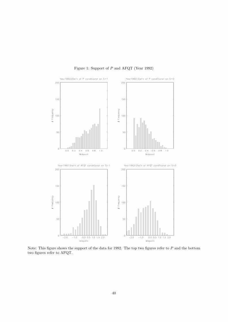
Figure 1: Support of P and AFQT (Year 1992)

Note: This figure shows the support of the data for 1992. The top two figures refer to P and the bottomtwo figures refer to AFQT.

40

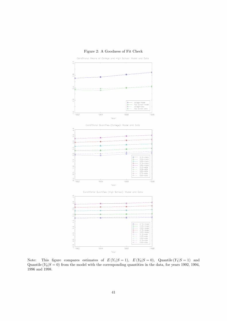
Figure 2: A Goodness of Fit Check

Note: This figure compares estimates of E (Y1|S = 1), E (Y0|S = 0), Quantile (Y1|S = 1) andQuantile (Y0|S = 0) from the model with the corresponding quantities in the data, for years 1992, 1994,1996 and 1998.

41

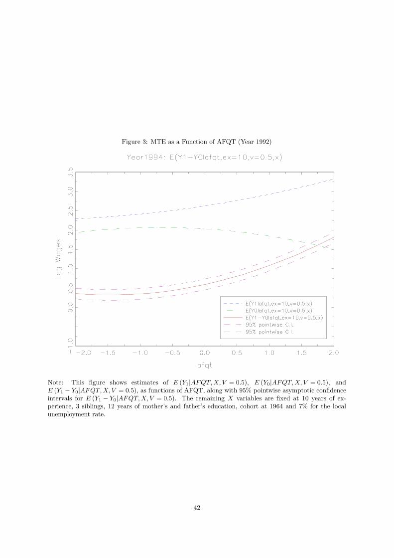
Figure 3: MTE as a Function of AFQT (Year 1992)

Note: This figure shows estimates of E (Y1|AFQT, X, V = 0.5), E (Y0|AFQT,X, V = 0.5), andE (Y1 − Y0|AFQT,X, V = 0.5), as functions of AFQT, along with 95% pointwise asymptotic confidenceintervals for E (Y1 − Y0|AFQT, X, V = 0.5). The remaining X variables are fixed at 10 years of ex-perience, 3 siblings, 12 years of mother’s and father’s education, cohort at 1964 and 7% for the localunemployment rate.

42

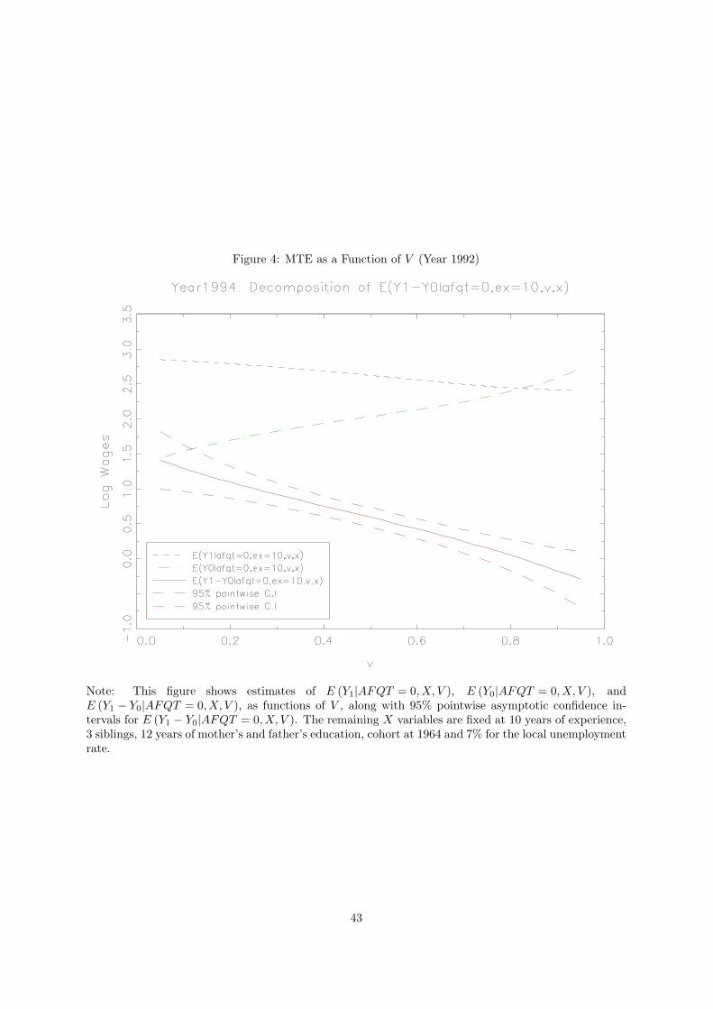
Figure 4: MTE as a Function of V (Year 1992)

Note: This figure shows estimates of E (Y1|AFQT = 0, X, V ), E (Y0|AFQT = 0, X, V ), andE (Y1 − Y0|AFQT = 0, X, V ), as functions of V , along with 95% pointwise asymptotic confidence in-tervals for E (Y1 − Y0|AFQT = 0, X, V ). The remaining X variables are fixed at 10 years of experience,3 siblings, 12 years of mother’s and father’s education, cohort at 1964 and 7% for the local unemploymentrate.

43

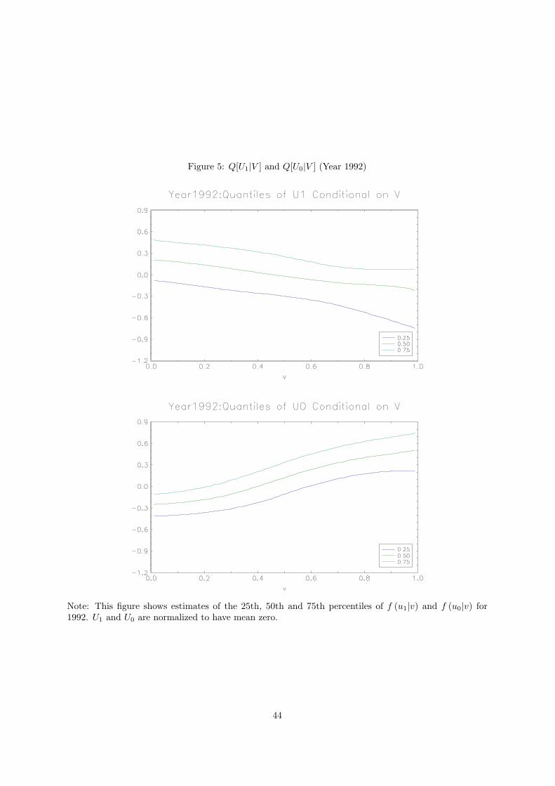
Figure 5: Q[U1|V ] and Q[U0|V ] (Year 1992)

Note: This figure shows estimates of the 25th, 50th and 75th percentiles of f (u1|v) and f (u0|v) for1992. U1 and U0 are normalized to have mean zero.

44

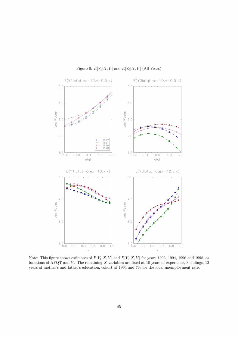
Figure 6: E[Y1|X, V ] and E[Y0|X, V ] (All Years)

Note: This figure shows estimates of E[Y1|X,V ] and E[Y0|X, V ] for years 1992, 1994, 1996 and 1998, asfunctions of AFQT and V . The remaining X variables are fixed at 10 years of experience, 3 siblings, 12years of mother’s and father’s education, cohort at 1964 and 7% for the local unemployment rate.

45