Wage Bargaining with On-the-job Search:A Structural Econometric Model1

Pierre CahucUniversité de Paris I, Paris,CREST-INSEE, Malakoff,

CEPR, London

Fabien Postel-Vinay2

INRA-Paris Jourdan, Paris,CREST-INSEE, Malakoff,

CEPR, London

Jean-Marc RobinUniversité de Paris I, Paris,CREST-INSEE, Malakoff,INRA Paris-Jourdan, Paris,

CEPR, London on

November 12, 2002

1Conversations with Bruno Crépon, Zvi Eckstein, Francis Kramarz and Barbara Petrongolo werehelpful for the preparation of this paper. The authors also wish to thank participants in the followingconferences and workshops: the CEPR DAEUP meeting in Paris (May 2002), the CEPR/IZA ESSLEmeeting in Buch an Amersee (Sept .2002), ERC conference in Chicago (Oct. 2002). The customarydisclaimer applies.

2Corresponding author: INRA Paris-Jourdan, Ecole Normale Superieure, 48 boulevard Jourdan75014 Paris, France. Email: fpostel@delta.ens.fr

on teOctober 2002, Preliminary

Abstract. We write and estimate an equilibrium model with strategic wage bar-gaining and on-the-job search and use it to take another look at the determinantsof wages in France. There are three essential determinants of wages in our model:productivity, competition between employers resulting from on-the-job search, andthe workers’ bargaining power. We find that between-firm competition matters alot in the determination of wages. In particular, we detect no significant bargainingpower for unskilled workers. However, inter-industry differentials are mainly due todifferences in productivity, and bargaining power, in the case of skilled workers.

1 Introduction

The empirical studies that estimate the impact of observable workers characteristics on wages

typically explain no more than 50% of the variation in compensation across individuals. On

the other hand, many empirical studies have shown that wage differentials are influenced by

differences in pay policies across firms (Abowd et al., 1999). These findings, which suggest

that similar workers employed in different firms can be paid differently, have fuelled a strand

of literature that stresses the importance of labor market frictions for understanding wage

determination (Mortensen, 2002, provides a recent survey). It is well known that by preventing

workers from bringing employers into Bertrand wage competition, search frictions give strictly

positive value to formed firm-worker pairs, and they also give some local monopsony power to

the firms. In this context, that is a rent sharing mechanism that explains why similar workers

are paid differently.

Models with search frictions have highlighted two reasons why workers can get some part

of the rents. The so-called matching model (Pissarides, 2000, Mortensen and Pissarides, 1999)

focuses on bilateral bargaining between firms and workers as the prevailing rent sharing mecha-

nism. In this model, wages are continuously renegotiated by Nash bargaining over the expected

match value. Even when on-the-job-search is allowed it is assumed that the worker who is

being offered an alternative to his or her current job takes the best outcome of two separate

Nash bargaining games, where the worker’s outside option is supposed to be unemployment,

so that on-the-job search does not give rise to beween-firm competition. In the wage post-

ing/equilibrium search models à la Burdett and Mortensen (1998), in which employers make

take-it-or-leave-it offers, on-the-job search leads employers to leave a part of the rents to their

employees in order to reduce labor turnover.

The principal argument of our paper is that the Bertrand competition paradigm, which is at

the root of the competitive model of wage formation, may have been too quickly abandoned.1

1A certain schizophrenia nonetheless persists in the profession as the competitive paradigm seems at least

1

There is little doubt that workers are unable to instantaneously or costlessly bring employers into

Bertrand wage competition, the outcome of which would be marginal productivity payment.

Search frictions limit competition and imperfect information about the location of available

employment opportunities, their scarcity, are definite sources of rent appropriation by firms.

Yet, limited competition does not mean absent competition.

In previous work, Postel-Vinay and Robin (2002a, 2002b) have explored this idea in a formal

equilibrium search model sharing many features with the models of Mortensen (1990) and Bur-

dett and Mortensen (1998), except that Postel-Vinay and Robin did not assume wage posting.

Wage posting models assume that firms make take-it-or-leave-it offers to workers and rule out

any possibility for employers to counter the attempts by competitors to poach their employ-

ees. Postel-Vinay’s and Robin’s model also assumes that firms make take-it-or-leave-it offers

to unemployed workers. The situation is different when an employee is contacted by another

employer because raising an outside offer is the means by which an employee can activate the

between-employer Bertrand competition. The incumbent employer and the poacher are forced,

by a well understood interest, to compete for the worker, this competition resulting either in

a wage raise or in a job mobility if the poacher’s reservation value (the match productivity) is

higher than the incumbent’s.

The present paper extends the equilibrium search model with sequential auctions of Postel-

Vinay and Robin by replacing Bertrand competition by a more general wage bargaining scheme

involving workers and all the incumbent and other would-be employers that are brought into

contact. In this perspective, we construct simple strategic bargaining games reflecting in a

stylized way the most prominent features of the negotiation and renegotiation of employment

contracts. Specifically, we make a sharp distinction between negotiation on new matches and

renegotiation on continuing jobs. The former always leads to severance in case of disagreement.

as widely accepted in other empirical segments of labor economics. Mincerian wage equations, supposed toexclusively reflect productivity differences, are indeed endorsed without restriction whatsoever by many majorempirical contributions ranging from Heckman’s various estimates of the Roy model, to dynamic discrete choicemodels, of which Keane and Wolpin (1994) is a perfect example.

2

The latter, started by employees receiving an outside offer, involves between-firm competition

and allows the parties to continue under the terms of the current contract in case of dis-

agreement. Our model thus explains why and when renegotiations occur and suggests that

negotiation and renegotiation put the parties in different situations.

This approach allows us to evaluate the separate contributions of between-firm competition

and the bargaining power on wages. This issue is important for many purposes. For instance,

according to the so-called Hosios-Pissarides condition, the labor market is efficient if the surplus

share accruing to workers takes a certain value, hinging on properties of the matching function

(Hosios, 1990, Pissarides, 2000). From this perspective, estimating the bargaining power is a

first step towards a proper evaluation of labor market efficiency. Also, reducing the workers’

bargaining power can be thought of as a policy to cut unemployment. A biased measure of this

bargaining power, that does not disentangle between-firm competition from wage bargaining

effects can cause the implementation of policies aiming at reducing the workers’ bargaining

power when it is not needed.

Related literature. Probably the paper most closely related to ours is Dey and Flinn (2000).

They represent the negotiation process by the Nash bargaining solution in the presence of

between-firm competition for workers. Their idea is that a worker who is currently employed at

a wage w0 and receives an outside offer bargains with the poaching firm on the basis that if the

negotiation fails the current wage contract w0 will prevail. Let w1 be the wage thus negotiated

with the poacher. In a second step, the worker uses this offer w1 as an outside option to nego-

tiate a new wage, w2, with his/her current employer. A sequence of bilateral Nash bargaining

games is played instantaneously until one of the firms can no longer bid up, that is when the

sequence of wage offers has reached the smallest firm reservation value or match productivity.

Our contribution provides an explicit non-cooperative bargaining game that relies on a pre-

cise definition of the strategic interactions at work in the wage renegotiation. Moreover, Dey

and Flinn consider a more complex framework, with multidimensional employment contracts

3

stipulating wages and health insurance provisions, that does not yield wage equations allowing

the estimation of the worker’s bargaining power. In our paper, we do estimate the bargaining

power using matched worker-firm panel data from France.2

The reader who is familiar with the early contribution of Eckstein and Wolpin (1995) will

understand that our work can also be viewed as an extension of theirs. Their paper is the

first paper that we know of that has proceeded to the estimation of a fully specified general

equilibrium model of wage bargaining on micro data. Eckstein andWolpin adapted the standard

Pissarides matching model to fit the micro data of the NLSY. One is then entitled to ask how

we shall be able to identify workers’ bargaining power when Eckstein and Wolpin claimed that

it was not possible to separately identify the location parameter of the distribution of match

productivities from the bargaining power parameter. This is because they used worker data and

did not observe match productivity separately from wages. We do not face this identification

problem as we use both worker and firm data, which will allow us to estimate a system of two

equations: a production function and a wage equation, allowing for a separate identification of

the parameters of the production function and the wage equation.

Outline and main results. In the following section of this paper, we develop formal non

cooperative negotiation and renegotiation games which allow us to express wages as functions

of worker ability, firm productivity, matching frictions and the bargaining power of workers.

Our first contribution is to provide closed-form expressions for wages and wage distributions

that hinge on these four elements in a unified theoretical model.

The empirical implementation of the model is presented in section 3. We use the frame-

work of section 2 to estimate the influence of productivity, between-firm competition and the

bargaining power of workers on wages. Because it is particularly important to separately iden-2An earlier, also closely related paper assumes that workers may not search sequentially. Burdett and Judd

(1982) show that if unemployed workers have a probability strictly between 0 and 1 of receiving more than onewage offer at a time, then the equilibrium wage distribution is necessarily dispersed even if all firms and workersare alike and even without on-the-job search.

4

tify the different sources of wage dispersion, we choose to implement a multi-stage estimation

procedure. We first estimate the friction parameters (arrival rate of job offers, job destruction

rate) from worker data on employment spell durations. We then use a firm panel of data on

value-added and employment differentiated by skill to estimate labor productivity at the firm

level. Lastly, we relate mean wages per firm to productivity to estimate bargaining powers.

Section 4 presents some empirical applications.

First, it is shown that ignoring on-the-job search causes substantial upwards biases in the

bargaining power estimates. In particular, we find that “unskilled” workers (workers with no

managerial tasks) have zero bargaining power in most industries whereas “skilled” workers

(supervisors, managers of all ranks and educated engineers) generally have positive bargaining

power, the extent of which varies across industries. This result suggests that most previous

empirical studies overestimated the bargaining power. These studies (a non exhaustive list

of the papers includes Abowd and Lemieux, 1993, Blanchflower et al., 1996, Van Reenen,

1996, Margolis and Salvanes, 2001, Kramarz, 2002), based on simple static models where some

bargaining process leads to splitting the job surplus, typically defined as the difference between

productivity and an outside wage that depends on worker characteristics and selected labor

market variables such as the (local) unemployment rate and the industry- or economy-wide

mean wage.

Then, we use our model to take another look at the determinants of inter-industry wage

differentials. There are three essential determinants of inter-industry wage differentials in our

model: productivity, between-firm competition, and the bargaining power. We find that, even

though taking account of job-to-job mobility matters in the determination of wages, inter-

industry differentials are mainly due to differences in productivity and bargaining power. It is

worth stressing that these results do not mean that between-firm competition does not influence

wages. Actually, our empirical results suggest that it does play a crucial role. However, it turns

out that the differences in the intensity of between-firm competition across industries, although

5

significant, explain a very small share of inter-industry wage differentials. In this section, we

also analyze inter-skill wage differentials and find, with no surprise, that skill wage differentials

essentially reflects productivity differences.

2 Theory

We first describe the characteristics and objectives of workers and firms. The matching process

and the negotiation game that workers and firms play to determine wages is then explained.

In the third and last subsection, the steady-state general equilibrium of this economy is char-

acterized.

2.1 Workers and firms

We consider a labor market in which a measure M of atomistic workers face a continuum of

competitive firms, with a mass normalized to 1, that produce one unique multi-purpose good.

Time is continuous, workers and firms live forever. The market unemployment rate is denoted

as u. The pool of unemployed workers is steadily fueled by layoffs that occur at the exogenous

rate δ.

Workers have different professional skills. A given worker’s ability is measured by the

amount ε of efficiency units of labor she/he supplies per unit time. The distribution of ability

values in the population of workers is exogenous, with cdf H over the interval [εmin, εmax]. We

only consider continuous ability distributions and further designate the corresponding density

by h.

Summing over all employee ability values for a given firm defines the efficient firm size.

The marginal productivity of efficient labor is denoted as p. Firms differ in the technologies

that they operate, meaning that parameter p is distributed across firms with a cdf Γ over the

support [pmin, pmax] . This distribution is assumed continuous with density γ. The marginal

productivity of the match (ε, p) of a worker with ability ε and a firm with technology p is εp.

A type-ε unemployed worker receives an income flow of εb, with b a positive constant,

6

which he has to forgo from the moment he finds a job. Being unemployed is thus equivalent to

working at a “virtual” firm with labor productivity equal to b that would operate on a frictionless

competitive labor market, therefore paying each employee their marginal productivity, εb.

Workers discount the future at an exogenous and constant rate ρ > 0 and seek to maximize

the expected discounted sum of future utility flows. The instantaneous utility flow enjoyed from

a flow of income x is U(x) = x.3 Firms maximize profits.

2.2 Matching and wage bargaining

Firms and workers are brought together pairwise through a sequential, random and time con-

suming search process. Specifically, unemployed workers sample job offers sequentially at a

Poisson rate λ0. As in the original Burdett and Mortensen (1998) paper, employees may also

search for a better job while employed. The arrival rate of offers to on-the-job searchers is λ1.

The type p of the firm from which a given offer originates is assumed to be randomly selected

in [pmin, pmax] according to a sampling distribution with cdf F (and F ≡ 1−F ) and density f .

The sampling distribution is the same for all workers irrespective of their ability or employment

status. Note that we a priori assume no connection between the probability density of sampling

a firm of given type p, f(p), and the density γ(p) of such types in the population of firms. When

a match is formed, the wage contract is negotiated between the different parties according to

the following rules.

2.2.1 Assumptions

Wages are bargained over by workers and employers in a complete information context. In

particular, all agents that are brought to interact by the random matching process are perfectly

aware of one another’s types. All wage and job offers are also perfectly observed and verifiable.

Specifically, we make the following three assumptions about wage strategies and wage contracts:

3This is merely for simplicity. The theoretical model is tractable with an arbitrary utility function (providedthat intertemporal transfers are ruled out), and the empirical analysis can in principle be conducted for anyCRRA specification (see Postel-Vinay and Robin, 2002).

7

Assumption A1 Wage contracts stipulate a fixed wage that can be renegotiated by mutual

agreement only.

Assumption A1 implies that renegotiations occur only if one party can credibly threaten

the other to leave the match for good if the latter refuses to renegotiate. In our framework,

renegotiations can be triggered only when employees receive outside offers. The assumption

of renegotiation by mutual agreement captures an important and often neglected feature of

employment contracts (see the enlightening survey by Malcomson, 1999).

The following two assumptions describe the structure of the negotiation game that is played

by an unemployed worker and an employer (Assumption A2), and that of the renegotiation

game that is played by a currently employed worker, his/her current employer and a poaching

employer (Assumption A3).

Assumption A2 When an unemployed worker meets a firm, the wage is determined according

to the following bargaining game:

1. The firm makes a wage offer;

2. The worker either accepts the offer and signs the contract, or s/he rejects it;

3. In case of rejection at step 2, some time elapses. Then:

• With probability β, the worker makes a wage offer;

• With probability 1− β, the firm makes a wage offer;

4. The player who has received the offer at step 3 either accepts it and signs the contract, or

rejects it. In case of rejection the match ends and the worker remains unemployed.

Assumption A3 An employed worker who receives an outside job offer renegotiates his/her

wage according to the following game:

1. The firms make simultaneous noncooperative wage offers;

8

2. The worker either chooses one wage offer and signs a new contract or keeps the pre-existing

contract;

3. If the worker has chosen one wage offer at step 2, some time elapses. Then the players

can participate in the following game:

• With probability β, the worker makes separate wage offers to both employers;

• With probability 1− β, the firms make simultaneous non-cooperative wage offers.

4. Any player who has received an offer at step 3 either accepts or rejects it. In case of

disagreement at step 4, the worker’s decision at step 2 prevails. In case of agreement

between the worker and either firm, a new contract is signed. The worker chooses among

the firms if both accept the offer s/he made at step 3.

Assumptions A2 and A3 describe two very simple strategic negotiation games adapted

from Osborne and Rubinstein (1990). The seminal contributions of Binmore, Rubinstein and

Wolinsky (1986) and Osborne and Rubinstein (1990) have shown that the Nash sharing rule can

be derived from strategic bargaining games that are very useful to properly define the threat

payoffs. Obviously, any strategic bargaining game is necessarily peculiar. Our game has been

designed to provide a simple and tractable tool to understand the renegotiation process in the

presence of between-firm competition for workers.

The negotiation game that is played between two firms and an initially employed worker

looks like the game between a firm and an unemployed worker except that the former has three

players instead of two. Steps 1 and 2 have been modified to enable the worker to maneuver

in order to get himself an optimal credible threat point in the renegotiation subgame (steps

3 to 4). Namely, if the worker accepts the offer of the poaching firm at step 2, he quits the

incumbent firm and this offer becomes his threat point in the renegotiation. Conversely, his

threat point is the offer of the incumbent employer if that offer is accepted at step 2. This

game can appear somewhat unrealistic at first glance, as it gives the employee the option to

9

momentarily quit the incumbent employer to eventually come back with a new contract at

the end of the renegotiation. Such back-and-forth worker movements don’t happen in the real

world. Neither do they in our game, as we wish to emphasize, since temporarily quitting to a less

attractive employer is only a threat available for the worker to use, which is never implemented

in equilibrium.

It is also worth insisting on the fact that whenever the worker receives an outside offer, the

pre-existing contract with the incumbent employer prevails if no agreement is reached (at step

2). This is an important difference with the negotiation on new matches–between unemployed

workers and firms–that are dissolved in case of disagreement. We view this assumption as

more in accordance with actual labor market institutions than the usual one according to

which matches always break up in case of renegotiation failure (Pissarides, 2000, Mortensen

and Pissarides, 1999). It is indeed legally considered in most OECD countries that an offer

to modify the terms of a contract does not constitute a repudiation. Accordingly, a rejection

of the offer by either party leaves the pre-existing terms in place, which means that the job

continues under those terms if the renegotiation fails (Malcomson, 1999, p. 2,321).

2.2.2 Wage contracts and job mobility

We now exploit the preceding series of assumptions to derive the precise values of wages and

the job mobility patterns.

The subgame perfect equilibria of the two bargaining games described above are character-

ized in Appendix A.1. In both games the worker receives a share β of the match rent. Let V0(ε)

denote the lifetime utility of an unemployed worker of type ε and V (ε, w, p) that of the same

worker when employed at a firm of type p and paid a wage w. The rent of a match between

a type-ε unemployed worker and a type-p job amounts to V (ε, εp, p) − V0(ε). It is shown in

the Appendix that the wage bargained on a match between a type-ε unemployed worker and a

10

type-p firm, denoted as φ0 (ε, p), solves:

V (ε,φ0(ε, p), p) = V0(ε) + β [V (ε, εp, p)− V0(ε)] . (1)

This equation merely states that a type-ε unemployed worker matched with a type-p firm gets

his reservation utility, V0(ε), plus a share β of the rent accruing to the job.

The assumption of long term contracts, renegotiated by mutual agreement only, implies

that wages can be renegotiated only if employees receive new job offers. Moreover, an employee

paid a wage w in a type-p firm and who receives an outside offer from a type-p0 firm is willing

to trigger a renegotiation only if firm p0 is competitive enough:

If p0 ≤ p, the worker stays at the type-p firm, because the match with the type-p0 firm is

associated with a lower rent. However, the employee can get wage increases if p0 is sufficiently

high in regard of his/her current wage, w. If the employee triggers a renegotiation (by accepting

the poacher’s first offer at step 2), he eventually stays at his initial firm (the type p firm) with

a new wage φ(ε, p0, p) as defined by:

V (ε,φ(ε, p0, p), p) = V (ε, εp0, p0) + β£V (ε, εp, p)− V (ε, εp0, p0)¤ . (2)

Obviously, the employee decides to trigger a renegotiation only if it is a way to get a wage

increase, i.e. if the productivity parameter of the new match, p0, exceeds a threshold value

q(ε, w, p), that satisfies:

φ(ε, q(ε, w, p), p) = w. (3)

Let us insist a bit on the role played by the game structure at this point. Note that

V (ε, εq(ε, w, p), q(ε, w, p)) = V (ε, w, p)− β

1− β[V (ε, εp, p)− V (ε, w, p)]

≤ V (ε, w, p)

(with strict inequality if w < p). The observant reader will thus have noticed that an outside

offer from a type p0 firm can result in a wage increase even when V (ε, εp0, p0) < V (ε, w, p),

i.e. even when the poacher’s productivity is so low that it can’t even afford to compensate the

11

worker for his/her pre-existing value V (ε, w, p). This results from the existence of steps 3 and

4, which ensure that the worker can credibly threaten to accept the weaker firm’s offer at step

2, even in cases where that offer is lower than what s/he would have gotten at status quo. In

other words, in order to force his/her incumbent employer to renegotiate, the worker is willing

to “take the chance” of accepting a very unattractive offer from the poacher because s/he knows

that it is then in the interest of her incumbent employer to attract him/her back with a wage

increase at later stages of the renegotiation game.

If p0 > p, the outside offer creates a (private) rent supplement equal to V (ε, εp0, p0) −

V (ε, εp, p). The renegotiation game thus implies that the worker moves to the type-p0 job,

where s/he gets a wage φ (ε, p, p0) that solves:

V (ε,φ(ε, p, p0), p0) = V (ε, εp, p) + β£V (ε, εp0, p0)− V (ε, εp, p)¤ . (4)

It can be seen that an employee who moves from a type-p to a type-p0 firm gets a value equal

to the maximum that s/he could get from staying at the type-p firm, plus a share β of the new

match rent. Note that the wage φ(ε, p, p0) obtained in the new firm can be smaller than the

wage w paid in the previous job, because the worker expects larger wage raises in firms with

higher productivity.

To sum up, one of the following three situations may arise when a type-ε worker, paid a

wage w by a type-p firm, receives a type-p0 job offer:

(i) p0 ≤ q(ε, w, p), and nothing changes.

(ii) p ≥ p0 > q(ε, w, p), and the worker obtains a wage raise φ (ε, p0, p) − w > 0 from his/her

current employer.

(iii) p0 > p, and the worker moves to firm p0 for a wage φ (ε, p, p0) that may be greater or

smaller than w.

Before we go any further, we should note that Dey and Flinn (2000) have reached similar

sharing rules to those just derived in a similar framework by applying the Nash bargaining

12

solution. Our contribution shows that this result can be derived from a precisely defined strategic

bargaining game compatible with job continuation when renegotiations fail.4

The precise form of wages can be obtained from the expressions of lifetime utilities (see

Appendix A.2 for the corresponding algebra). The wage φ (ε, p0, p) of a type-ε worker, currently

working at a type-p firm and whose last job offer was made by a type-p0 firm, is defined by:

φ¡ε, p0, p

¢= ε ·

µp− (1− β)

Z p

p0

ρ+ δ + λ1F (x)

ρ+ δ + λ1βF (x)dx

¶. (5)

This expression shows that the returns to on-the-job search depend on the bargaining power

parameter β. It can be seen that outside offers trigger wage increases within the firm only if

employers have some bargaining power. In the limiting case where β = 1, the worker appropri-

ates all the surplus up-front and gets a wage equal to εp, whether or not s/he searches on the

job. In the opposite extreme case, where β = 0, the wage increases as outside offers come since

all offers from firms of type p0 ∈ (q(ε, w, p), p] provoke within-firm wage raises.

The wage φ0(ε, p), obtained by a type-ε unemployed workers when matched with a type-p

firm, writes as:

φ0(ε, p) = ε ·µpinf − (1− β)

Z p

pinf

ρ+ δ + λ1F (x)

ρ+ δ + λ1βF (x)dx

¶, (6)

where pinf is the lowest viable marginal productivity of labor. The latter is defined as the

productivity value that is just sufficient to compensate an unemployed worker for his forgone

value of unemployment, given that he would be paid his marginal productivity, thus letting the

firm with zero profits. Analytically:

V (ε, εpinf , pinf) = V0 (ε)

m

pinf = b+ β(λ0 − λ1)

Z pmax

pinf

F (x)

ρ+ δ + λ1βF (x)dx (7)

4Moreover, Dey and Flinn focus on the renegotiation issue in a more complex framework with multidimensionalemployment contracts stipulating wages and health insurance provisions. Due to this added complexity, they areunable to come up with closed-form expression for wages and wage distributions.

13

It appears that pinf differs from the unemployment income if workers have positive bargaining

power. For instance, εpinf is greater than the unemployment income flow εb if the arrival rate

of job offers to unemployed workers λ0 is larger than the arrival rate to employees, λ1. In

that case, accepting a job reduces the efficiency of future job search. The worker needs to be

compensated for this loss through a wage higher than his unemployment income. Operating

firms thus have to be able to afford wages at least equal to pinf , which imposes the obvious

condition that they be at least as productive as pinf . It is worth noting that the lower support

of observed marginal productivities, that we denote by pmin, can be strictly above the lower

support of viable productivities pinf , for instance if free entry is not guaranteed on the search

market.

The definition (6) of φ0(ε, p) together with the definition (7) of pinf shows that entry wages,

received by individuals who exit from unemployment, are not necessarily higher than the un-

employment income. It actually appears that those wages are always smaller than the unem-

ployment income if workers have no bargaining power, because accepting a job is a means to

obtain future wage raises. Entry wages obviously increase with the bargaining power parameter

β.

We end this Section by some comments on comparative statics. The wage function φ(ε, p, p0)

decreases with λ1 and F (with respect to first-order stochastic ordering), and increases with

δ. These properties reflect an option value effect: workers are willing to pay for higher future

propects. Of course φ(ε, p, p0) increases with bargaining power, β. The wage function is an

increasing function of worker ability ε and the type p of the less competitive employer, as

both Bertrand competition and Nash-bargaining work in tandem to push wages up. However,

we note an ambiguous effect of the type p0 of the employer winning the auction: φ(ε, p, p0)

decreases with p0 if β is small enough for the option value effect to dominate. A high p0 means

that the upper bound put on future renegotiated wages is more remote (as it is equal to p0) and

the worker is thus willing to trade lower present wages for a promise of higher future wages.

14

However, φ(ε, p, p0) increases with p0 if β is large enough for the bargaining power effect on rent

sharing to take over the option value effect.

2.3 Steady-state equilibrium

We know from what precedes that a type ε employee of a type p firm is currently paid a wage

w that is either equal to φ0(ε, p) = φ(ε, pinf , p), if w is the first wage after unemployment, or is

equal to φ(ε, q, p), with pinf ≤ pmin < q ≤ p, if the last wage mobility is the outcome of a bargain

between the worker, the incumbent employer and another firm of type q. The cross-sectional

distribution of wages therefore has three components: a worker fixed effect (ε), an employer

fixed effect (p) and a random effect (q) that characterizes the most recent wage mobility. In

this section we determine the joint distribution of these three components.

In a steady state a fraction u of workers is unemployed and a density `(ε, p) of type-ε workers

is employed at type-p firms. Let `(p) =R εmaxεmin

`(ε, p)dε be the density of employees working at

type-p firms. The average size of a firm of type p is then equal to M`(p)/γ(p). We designate

the corresponding cdfs with capital letters L(ε, p) and L(p), and we let G(w|ε, p) represent the

cdf of the (not absolutely continuous, as we shall see) conditional distribution of wages within

the set of workers of ability ε within type-p firms.

We now proceed to the derivation of these different distributional parameters by increasing

order of complexity. The steady state assumption implies that inflows must balance outflows

for all stocks of workers defined by a status (unemployed or employed), a personal type ε, a

wage w, an employer type p. The relevant flow-balance equations are spelled out in Appendix

A.3. They lead to the following series of definitions/results:

• Unemployment rate:

u =δ

δ + λ0. (8)

• Distribution of firm types across employed workers: The fraction of workers employed at

15

a firm with mpl less than p is

L(p) =F (p)

1 + κ1F (p), (9)

with κ1 =λ1δ , and the density of workers in firms of type p follows from differentiation as

` (p) =1 + κ1£

1 + κ1F (p)¤2 f (p) . (10)

• Distribution of matches: The density of matches (ε, p) is

`(ε, p) = h(ε)`(p). (11)

• Within-firm distribution of wages: The fraction of employees of ability ε in firms with mpl

p is

G (w|ε, p) =µ

1 + κ1F (p)

1 + κ1F [q (ε, w, p)]

¶2=

µ1 + κ1L [q (ε, w, p)]

1 + κ1L(p)

¶2. (12)

where q (ε, w, p), defined equation (3), stands for the threshold value of the productivity of

new matches above which a type-ε employee with a current wage w can get a wage increase.

Equation (8) is standard in equilibrium search models (see Burdett and Mortensen, 1998)

and merely relates the unemployment rate to unemployment in- and outflows.

Equation (9) is a particularly important empirical relationship as it will allow us to back

out the sampling distribution F from its empirical counterpart L.5

Equation (11) implies that, under the model’s assumptions, the within-firm distribution of

individual heterogeneity is independent of firm types. Nothing thus prevents the formation of

highly dissimilar pairs (low ε, high p, or low p, high ε) if profitable to both the firm and the

worker. This results from the assumptions of constant returns to scale, scalar heterogeneity

and undirected search.

Finally, equation (12) expresses the conditional cdf of wages in the population of type ε

workers hired by a type p firm. What the pair of equations (11,12) shows is that a random5It is exactly the same equilibrium relationship as between the distribution of wage offers and the distribution

of earnings in the Burdett and Mortensen model.

16

draw from the steady-state equilibrium distribution of wages is a value φ(ε, q, p) where (ε, p, q)

are three random variables such that

(i) ε is independent of (p, q),

(ii) the cdf of the marginal distribution of ε is H over [εmin, εmax],

(iii) the cdf of the marginal distribution of p is L over [pmin, pmax], and

(iv) the cdf of the conditional distribution of q given p is eG(·|p) over {pinf}∪ [pmin, p] such thateG(q|p) = G (φ(ε, q, p)|ε, p)

=

£1 + κ1F (p)

¤2£1 + κ1F (q)

¤2for all q ∈ {pinf}∪[pmin, p]. The latter distribution has a mass point at pinf and is otherwise

continuous over the interval [pmin, p].

3 Estimation

In this section, we describe the data and the estimation procedure and discuss the results.

3.1 Data

We use a dataset constructed by Crépon and Desplatz (2002). This dataset covers the period

1993-1997 and contains various accounting informations drawn from the BRN firm-data source

(“Bénéfices Réels Normaux”), collected by the French National Statistical Institute (INSEE) :

total compensation costs, value added, current operating surplus, gross productive assets, etc.,

plus an Auerbach-type measure of the user cost of capital computed by Crépon and Desplatz

using data on the age of capital. The BRN data are supposedly exhaustive of all private enter-

prises (not establishments) with a sales turnover of more than 3.5 million FRF (about 530,000

Euros) and liable to profit tax.6 Note that the necessary “cleaning” of this administrative data

source (mainly outlier detection and construction of the capital cost variable) let them retain6The BRN is a subset of a larger firm sample, the BIC, “Bénéfices Industriels et Commerciaux”.

17

only about 30% of all the firms present in the original sample (87,371 firms). In addition,

Crépon and Desplatz used the DADS worker data source (“Déclarations Annuelles de Données

Sociales”) to compute labor costs and employment, at the enterprise level, for different worker

categories (skill, age, sex). The DADS data are based on mandatory employer (establishments)

reports of the earnings of each salaried employee of the private sector subject to French payroll

taxes over one given year. This very large dataset was thus “collapsed” by enterprise and skill

category and then merged with the BRN dataset.7

Aggregating worker wages and labor into two skill categories (“skilled” and “unskilled”)8

we have formed four panels of firm data on value-added, employment by skill and average wage

by skill, covering the period 1993-1997 and corresponding to the following thirteen distinct

industries:

1. Intermediate goods2. Investment goods3. Consumption goods4. Electrical & electronic equipment

Manufacturing5. Construction6. Transportation

7. Wholesale, food8. Wholesale, nonfood9. Retail, food10. Retail, nonfood

Trade11. Automobile repair & trade12. Hotels & restaurants13. Personal services

ServicesTable 1 contains some descriptive statistics for the selected variables. We note that a large

majority of workers in every industry are unskilled, the proportion of unskilled workers rang-

ing from 57% (Wholesale, nonfood) to 81,8% (Construction). Moreover, the skilled-unskilled

average annual compensation cost ratio ranges between 1.5 (Hotel & Restaurants) and 2 (In-

termediate goods, Wholesale-food).7For more information on these datasets, we refer to the paper by Crépon and Desplatz and to Abowd,

Kramarz and Margolis (1999) for another very precise description of the same data sources and others.8The unskilled category comprises unskilled manual workers and trade employees. The skilled category

comprises skilled manual workers, administrative employees (secretaries, ...), engineers, and all employees withsome managerial function in the firm.

18

< Table 1 about here. >

Finally, estimating the model requires data on worker mobility. We use the French Labor

Force Survey (“Enquête Emploi”) which is a three-year rotating panel of individual professional

trajectories similar to the American CPS (“Current Population Survey”). We prefer to use the

LFS panel instead of the larger DADS panel as the latter is known to be affected by large

attrition biases. Moreover, the LFS is precisely designed to study unemployment and worker

mobility.

3.2 Productivity

The values and distribution of firms’ marginal productivity values p are crucial determinants

of wages in the structural model. Since these values are not directly observed in the data, their

construction is a key step in the estimation procedure. A central principle that we want to

stick with in the design of this procedure is that the productivity parameters p should not be

constructed to a priori fit the wage data, but should rather be identified from value-added data

alone. This, we believe, is the only way to get credible estimates of the bargaining power β,

which in turn will be identified by the connection that exists in the data between wages and

productivity.9

The construction of the p’s and their distributions for each labor category from value-added

data requires some additional structure on the production technology.

Further assumptions on the production technology. The population of workers is clus-

tered into two statistical categories called “skilled” and “unskilled”. We assume that each cat-

egory of workers faces the same transition rate values denoted as δs,λ0s,λ1s (resp. δu,λ0u,λ1u)

for, respectively, skilled and unskilled workers. Idem for the values of non market time bs and

bu.

9 It is therefore essential that our dataset contain information on both individual wages and value-added. Inthe absence of the latter, Postel-Vinay and Robin (2002b) had to rely on the sole wage data to construct the p’susing the structural relationship implied by the model between p and the conditional mean wage E (w|p).

19

Moreover, the observed skill type does not necessarily capture all the productive hetero-

geneity of workers. Specifically, there are Ms skilled workers and Mu unskilled workers in the

economy, with corresponding densities of professional ability hs(ε) and hu(ε) respectively.10

Firms’ labor input is an aggregate of skilled and unskilled labor constructed as follows. Let

Mj = Msj +Muj be the size of some firm j, comprising Msj observationally skilled workers

and Muj observationally unskilled. Letting hsj (ε) (resp. huj (ε)) denote the density of type-ε

skilled (resp. unskilled) workers employed at some firm j, the total amount of efficient labor

employed at this firm is

Lj =Msj

Zεhsj (ε) dε+Muj

Zεhuj (ε) dε. (13)

We then specify firm j’s total per-period output (value-added) as:

Yj = θjLξj , (14)

where θj is a firm-specific productivity parameter (that possibly captures heterogeneity in fixed

capital stocks), and ξ is between 0 and 1 and is also common to all firms.11

It is evident from equation (14) that the marginal value to firm j of a worker with ability ε

is pjε ≡ εξθjLξ−1j = εξYj/Lj , irrespective of his/her observed skill type. Of course one expects

that the statistical skill category is correlated with the true ability and that the mean ability

of unskilled workers is less than the mean ability of skilled workers:

αu ≡Z

εhu (ε) dε ≤ αs ≡Z

εhs (ε) dε. (15)

Assuming that the markets for observationally skilled and unskilled workers are perfectly seg-

mented, then, according to the theory laid out in the preceding section, there is no sorting

within each observationally homogeneous category of workers:

hsj (ε) = hs (ε) and huj (ε) = hu (ε) . (16)10Both densities may have disconnected supports, meaning hu(ε) · hs(ε) = 0 for all ε, in which case the

observable skill variable would indeed allow to partially sort workers by effective ability ε.11Note that we completely neglect the sort of externality problems pointed out by Stole and Zwiebel (1996),

Wolinsky (2000) and Cahuc and Wasmer (2001) resulting from diminishing marginal returns to labor. Withnonconstant returns to scale, the hiring decisions of firms affect their levels of productivity, and consequentlytheir labor costs. We simply assume that the firms’ hiring decisions are exogenous.

20

Hence

Lj = αuMsj + αsMuj (17)

and the average marginal productivity of a match between firm j and an unskilled (resp. skilled)

worker is αupj = αuξYjLj= αuξθjL

ξ−1j (resp. αspj). Also, because one can multiply ε by any

constant and divide θj by this constant indifferently we shall normalize the distribution of θj

so that αu =Rεhu (ε) dε = 1 and shall write α for the mean productivity ratio: αs

αu(= αs if

αu = 1).

Lastly, equation (10) in Section 2.3 gives the following expression for firm sizes:

Mkj =1 + κ1k£

1 + κ1kF k(pj)¤2 · fk (pj)γ (pj)

for k = s or u, (18)

where κ1k = λ1k/δk, where Fs (p) (resp. Fu (p)) are the sampling distributions of pj ’s in the

populations of skilled and unskilled workers, respectively, and where γ (p) (resp. Γ(p)) is the

density (resp. cdf) of pj ’s in the population of firms.

Estimation of the production technology. The production equation that we take to the

data is the following logged version of (14):

yjt = ln θj + ξ ln (Mujt + αMsjt) + ηjt, (19)

where yjt is the log value-added of firm j at date t,Mujt (resp. Msjt) is the number of unskilled

(resp. skilled) workers employed by firm j at date t, and ηjt is an error term independent of

the fixed effect ln θj .

We also posit the following empirical relationship between date-t employment and its steady-

state counterpart:

lnMkjt = lnMkj + ωkjt, (20)

with ωkjt an error term independent of θj . This last equation points at two potential sources

of endogeneity of Mkjt in (19): one is the correlation between Mkj and θj , and the other is the

possible correlation between ηjt and ωkjt.

21

Results. We estimate equation (19) by GMM under the following sets of moment restrictions:

∆ηjt ⊥nlnMkj,t−τ ; (lnMkj,t−τ )2 ; lnMsj,t−τ · lnMuj,t−τ

o, τ ≥ 2, (21)¡

ln θj + ηjt¢ ⊥ n

∆ lnMkj,t−τ ; (∆ lnMkj,t−τ )2 ;∆ lnMsj,t−τ ·∆ lnMuj,t−τo, τ ≥ 2. (22)

The set (21) of moment restrictions correspond to the estimation of the first-differenced model

instrumented by lagged values of the RHS variables dated at least t−τ . It is implicitly assuming

that ηjt is orthogonal to the past of ωkj,t−τ+1. The set (22) of moment restrictions adds the

restrictions which validates the estimation of the model in levels instrumented by lagged values

of first-differenced RHS variables. Lastly, assuming these restrictions valid for all τ ≥ 2 is like

assuming that the random components ηjt and ωkjt are at most moving averages of order one.

We also tried estimating the model using the subset of restrictions for τ ≥ 3 (the most that

we can do with a five-year panel) and found no significant differences between both sets of

estimates.12

The GMM estimation results of equation (19) are gathered for our 13 sectors in Table 2.

< Table 2 about here. >

The first thing we notice is that the point estimates of the productivity ratio, α, are always

above 1, and almost always significantly so. The productivity ratio is highest in Manufacturing

and Transportation, closely followed by Trade and Personal services. This ratio is somewhat

lower in the sectors of Construction, Hotels and Automobile trade. The ordering that emerges

from our estimates of α roughly parallels wage ratios (see Table 1).

3.3 Worker mobility

Another key determinant of wages is the parameter κ1 = λ1/δ, which measures the average

number of outside job offers a worker receives between two unemployment spells. Since outside12Chamberlain (1992) validates these estimation procedures, which are inspired by Arellano and Bond (1991)

and Arellano and Bover (1995) and are applied to the nonlinear model (19). Chamberlain shows how a polynomialexpansion of the set of instrumental variables (or via any L2-complete sequence of functions) provides a sequenceof estimators approximately attaining the information bound.

22

job offers are the source of wage increases in the model, we expect that more “mobile” workers

(those with higher values of κ1) should on average exhibit steeper wage-tenure profiles. However,

what κ1 essentially determines is the duration of job spells. The same identification principle

applies here also. We want the estimation of κ1 to be as robust as possible as far as wage

distributions are concerned. We shall thus identify κ1 exclusively from job duration data rather

than wage data which would certainly buy us sizeable efficiency gains but would also increase

the risk of misspecifications biases.

As all job transition processes are Poisson, all corresponding durations are exponentially

distributed.13 In this Section we are interested in the distribution of job spell durations t, which

have the following density, conditional on p:

L (t|p) = £δ + λ1F (p)¤ · e−[δ+λ1F (p)]t, (23)

where we know from equation (10) that p is distributed in the population of employed workers

according to the density:

` (p) =1 + κ1£

1 + κ1F (p)¤2f (p) .

Because it is impossible to match the LFS worker data with the BRN firm data, we shall treat

p as an unobserved heterogeneity variable, that is: we integrate out p from the joint likelihood of

p and t, ` (p)L (t|p), and maximize the unconditional likelihood, L (t) = R pmaxpmin` (p)L (t|p) dp,14

to get an estimate of δ and κ1. This method of unconditional inference applied to labor

market transition parameters was first explored by van den Berg and Ridder (2000). As we

already mentioned, it has the additional advantage of yielding estimates of the transition rate

parameters that are robust to any specification error in the estimation of the productivity

parameters θj for all firms j.

The unconditional ML estimates of δ, λ1 and, most importantly, κ1 are reported in Table13 In practice we have to take into account the fact that the panel covers a fixed number of periods so that some

job durations are censored. It is easy to account for such right censoring. Moreover, the unconstrained likelihoodcan be analytically developed into simple combinations of exponentials and exponential-integral functions.14Simple calculations show that L (t) = R 1+κ1

1δ(1+κ1)

κ1

e−δxtxdx.

23

3. Since those estimates were obtained from LFS data, the relatively small number of observa-

tions forced us to aggregate our eleven sectors into five “broader” industries: Manufacturing,

Construction, Transportation, Trade, and Services.

In terms of κ1, i.e. the average number of outside contacts that an employed worker can

expect before the next unemployment shock, skilled workers are always more mobile than

unskilled workers. Now looking at the sheer frequency of such contacts, which is measured by

λ1, again we find that skilled workers get more frequent outside offers than unskilled workers,

except in Services and Transportation where the difference between the two labor categories is

in favor of the unskilled (although probably not significantly so in the Service sector). Finally,

the rate of job termination δ is everywhere higher for the unskilled than for the skilled.

< Table 3 about here. >

The average duration of an employment spell (i.e. the average duration between two unem-

ployment spells), 1/δ, ranges from 10 to 36 years, while the average waiting time between two

outside offers, 1/λ1, lies between 3.3 and 17 years. The average number of outside contacts, κ1,

that results from these estimates is never very large (between 1.34 and 5.28) which confirms

the relatively low degree of worker mobility in the French labor market. Workers are relatively

less mobile in Manufacturing and Transportation than elsewhere, where they tend to have both

lower job separation and job-switching rates. Concerning the Transportation sector, the rela-

tively large share of State-owned companies in this industry may explain that result. Unskilled

worker turnover is remarkably higher in Services, probably due to the relatively more frequent

use of fixed-term contracts in that sector.15

3.4 The wage equation

We now turn to the last step of our estimation procedure, in which we combine the wage data

with our productivity parameter estimates from step 1 to estimate a wage equation, which will15The average stock percentage of fixed-duration contracts in our LFS sample is 4.6% in Construction, 5.5%

in Trade, 4.3% in Manufacturing, and as high as 16.3% in Services.

24

identify the workers’ bargaining power β.

Given our knowledge of wage determination (equation (5)) and the (conditional) wage distri-

bution (equation (12)), we can derive the conditional mean wage E (w|p) for each skill category

(skilled and unskilled),16 the empirical counterpart of which is the firm-level average wage.

Equation (A16) in the Appendix shows that:

E (w|p) = E (ε) ·Ãp−

£1 + κ1F (p)

¤2(1 + κ1)

2

Z εmax

εmin

[φ (ε, pmin, p)− φ (ε, pinf , p)]h(ε)dε

− £1 + κ1F (p)¤2 Z p

pmin

(1− β)£1 + (1− σ)κ1F (q)

¤£1 + (1− σ)κ1βF (q)

¤ £1 + κ1F (q)

¤2dq!.

This expression can be further simplified. First, we should take account of the fact that E (ε) = α

(αs or αu depending on which skill category we consider) is estimated in step 1 together with

pj for all firms. Second, we can notice that if the lower support of viable productivities pinf

equals the lower support of observed productivities pmin (which amounts to assuming free entry

and exit of firms on the search market), then the second term in the right hand side vanishes.

We shall henceforth adopt this assumption.17 We thus now have:

E (w|p) = α

Ãp− £1 + κ1F (p)

¤2 Z p

pmin

(1− β)£1 + (1− σ)κ1F (q)

¤£1 + (1− σ)κ1βF (q)

¤ £1 + κ1F (q)

¤2dq!. (24)

With equation (10) implying that F (p) = (1+κ1)L(p)1+κ1L(p)

, our knowledge of κ1 and of the value of p

for each firm let us construct F (p) using the empirical cdf of pj ’s in the population of workers

to estimate L (p).

Letting wkjt denote the observed firm-level mean wage of labor category k (= s or u), at

date t, in firm j, we obtain a value of βk (the bargaining power of workers of category k) by

fitting the theoretical mean wage E³w|bpj ; bFk, bαk, bκ1k,βk´ that one computes using (24) to wkjt

using (weighted) nonlinear GLS.18

Table 4 displays the estimated values of β for each category of labor. Also, the two panels

in Figure 1 plot the predicted and observed wages against the empirical cdf Γ (p) for one of16To simplify the notation, we shall omit in this section the skill index “s” or “u”.17Unconstrained estimations always lead to the conclusion that pinf indeed equals pmin.18We also need a value for the discount rate ρ which appears in σ = ρ/ (ρ+ δ). We normalize it for everyone

to an annual value of 0.15.

25

the 13 sectors under consideration (we took the first sector in the list–the Intermediate goods

industry–as our example). A glance at those Figures shows that the model is reasonably good

at predicting wages, given the fact that we only had one free parameter (β) to fit wage data.

< Table 4 about here. >

< Figure 1 about here. >

Concerning the values of β reported in Table 4, one can make the following general com-

ments. Unskilled workers have a very low bargaining power in most sectors. Their bargaining

power amounts to zero in 9 out of 13 sectors. Skilled workers have bargaining powers that are

significantly larger than those of unskilled workers. The range of βs’s is very large, going from 0

(Personal services) to 0.83 (Automobile repair & trade) and their values are very heterogeneous.

4 Applications

In this section, we use our framework to shed light on three issues. First, we disentangle

the respective influence of the bargaining power and the between-firm competition on wage

distribution within each sector. Then, we analyse the inter-industry wage differentials and the

returns to qualification.

4.1 Assessing the importance of between-firm competition

As we argued in the Introduction, the conventional approach to evaluating the workers’ bar-

gaining power ignores job-to-job mobility. Our model offers a simple way of assessing the bias

in the estimation of β resulting from this simplification. Ignoring job-to-job mobility indeed

amounts to forcing κ1 = 0 in the wage equation (24) that now reads

E (w|p,κ1 = 0) = β0αp+ (1− β0)αpmin. (25)

We obtain an estimator of the bargaining power in the absence of on-the-job search, bβ0, usingweighted NLS19 separately for each industry and skill. It is important to note that this estimate19All estimates reported in Table 5 were obtained by WNLS using the log-version of equation (25) and the

same metric as for the estimation of the wage equation with OTJ search (which is the optimal metric for the

26

bβ0 is a measure of the mean worker share of match rent, E (E (w)− αpmin) /E (αp− αpmin).

The values of bβ0 are gathered in the first two columns of Table 5. Comparing the bargainingpower estimates with and without on the job search–i.e. comparing the values of bβ0 to thevalues of β from Table 4–immediately shows that the bargaining power is always overestimated

when one ignores job-to-job mobility. The magnitude of this upward bias varies across skill

groups and sectors, but the bias always seems to be there, and is always important. This

was expected as on-the-job search is a means by which an employee can force her employer

to renegotiate her wage upward. Neglecting on-the-job search biases the workers’ bargaining

power upward to make it fit the actual share of compensation costs in value-added.

Table 5’s columns 3 and 4 report estimates bbβ0 of the mean worker share of match rents ob-tained from predicted (rather than observed) firm level mean wage data. That is, we simulated

firm mean wages using our set of parameter estimates, and re-ran the estimation of equation

(25) using those data. As can be seen by comparing the values bβ0 and bbβ0, we generally tendto overestimate wages a bit, especially so for unskilled workers in Construction, Retail Trade

and Automobile Services.20 Simulated and observed data otherwise produce reasonably similar

results.

What we want to know next is how much of this estimated bbβ0 is explained by “noncom-petitive wage setting” (i.e. the bargaining power that workers may have), versus how much of

it is due to between-firm competition. What we are looking for here is another answer to the

question of knowing to what extent do we need an extra rent sharing device (in addition to

between-firm competition) to explain wages. To find this answer we simulate new wage data,

again using our parameter estimates everywhere except for β, that we force to equal zero. That

is, we produce the wage data that one would collect from the French labor market if French

workers had no bargaining power at all, i.e. if the only source of rent acquisition by workers

latter regression). The reason why we use the same metric for all estimates is just consistency, as the quantitativeresults tend to be mildly sensitive to the metric used for some particular industries. Different choices of metrichave no qualitative impact.20This will be confirmed by a more precise look at the wage prediction error in Table 6.

27

were between-employer competition. That being done, we estimate equation (25) using this

last set of wage data, and compare the rent share obtained to bbβ0. This tells us how much of bbβ0is explained by between-firm competition alone.

The results are in the last two columns of Table 5. Clearly, competition between firms

explains one hundred percent of the workers’ share of match rents everywhere where the bar-

gaining power β was estimated to be zero. What that means is that between-firm competition

alone is enough to explain unskilled wages in practically all industries. What we also find from

looking at the last “Skilled” column of Table 5 is that the rent share acquired by skilled work-

ers is also largely explained by between-employer competition. Even though we undoubtedly do

need some noncompetitive wage formation device such as wage bargaining to reproduce skilled

wages, sheer labor market competition explains way over half (in fact, over 70% on average if

one believes the figures in Table 5) of the rents accruing to these workers.

4.2 Inter-industry wage differentials.

Going back to the theoretical model, one can derive the market-average (real) wage by simply

integrating the conditional mean wage (24) with respect to the distribution of workers across

firms (10):

E (w|p;F,α,κ1,σ,β) = αpmin

+ α (1 + κ1)

Z pmax

pmin

F (x)

1 + κ1F (x)·Ã1− (1− β)

£1 + κ1 (1− σ)F (x)

¤£1 + βκ1 (1− σ)F (x)

¤ £1 + κ1F (x)

¤! dx. (26)

This obviously depends on the entire set of structural parameters, which are specific to each

sector and labor categories. According to our structural model, inter-sectoral differences in

mean wages reflect differences in this set of structural parameters, which of course includes the

workers’ bargaining power β, but also worker mobility parameters (κ1 and δ), and “productivity

effects” (worker productivity parameters αu and αs, the returns to labor ξ and the distributions

of firm fixed-effects θj). A natural question to ask is then which parameters in that set are

most important in determining inter-industry wage differences.

28

There is no unique or straightforward way to answer this question.

First, it can be noticed that the consequences of productivity differences are straightforward

since mean wages are proportional to any scale factor of the production function. Hence, raising

the productivity of all firms of a sector by one percentage point raises the market mean wage

of that sector–in fact, it raises all firm-level mean wages–by one percentage point. Note that

a crucial assumption for this result is that the efficiency of job search (as measured by λ1) be

independent of the firms’ types, which wouldn’t generically be the case if one were to endogenize

e.g. the workers’ search efforts (see Christensen et al, 2001).

We can also shed some light on the impact of other variables by looking at the “sensitivity”

of the predicted mean wage to changes in a series of structural parameters. Specifically, we

consider shifting two distinct parameters: the bargaining power β, and the “worker mobility”

parameter κ1, which can be interpreted as a measure of how far away our labor market is from

the Walrasian paradigm, as wages equal the marginal productivities of labor whose distribution

degenerates to a mass point when κ1 →∞.We then proceed to the computation of the predicted

log average wage for each sector/skill category:

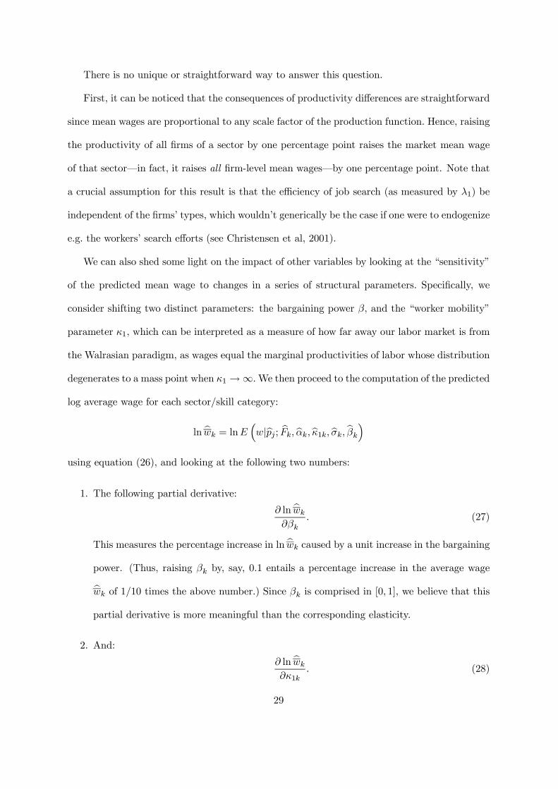
ln bwk = lnE ³w|bpj ; bFk, bαk, bκ1k, bσk, bβk´using equation (26), and looking at the following two numbers:

1. The following partial derivative:

∂ ln bwk∂βk

. (27)

This measures the percentage increase in ln bwk caused by a unit increase in the bargainingpower. (Thus, raising βk by, say, 0.1 entails a percentage increase in the average wagebwk of 1/10 times the above number.) Since βk is comprised in [0, 1], we believe that thispartial derivative is more meaningful than the corresponding elasticity.

2. And:

∂ ln bwk∂κ1k

. (28)

29

Similarly, this measures the percentage increase in ln bwk caused by a unit increase inκ1k. We also think this is a natural number to look at (rather than the corresponding

elasticity), since what κ1k measures is the average number of contacts with an outside

potential employer that a worker makes between two unemployment spells (i.e., according

to Table 3, over a typical period of 1/δk ' 20 years). The above number therefore tells

the percentage increase in bwk that one should expect if workers were to get one extraoutside offer on average every 1/δk years.

Table 6 contains the corresponding numbers for each of our thirteen sectors. The first column

in that Table reports the empirical log average wage lnw. The second column shows the log

average wage ln bw predicted by equation (26) and the parameter estimates obtained earlier.

Column 3 reports the prediction error. The following two columns contain our two numbers

of interest (27) and (28) computed using our set of estimates.21 Finally, the last two columns

show the values taken by (27) and (28) under the assumption of no on-the-job search, i.e. with

κ1 = 0 and β taking the values bβ0 from the first two columns of Table 5. We now comment on

the figures contained in Table 6.

< Table 6 about here. >

Column 4 in Table 6 contains a measure of the sensitivity of average wages to changes in

the bargaining power of workers. What those numbers tell us is that if one were to increase the

bargaining power of all workers by, say, 0.1, then average wages would be increased by roughly

2.5 to 8 percentage points, depending on the sector and worker category. Also, as can be seen

from a comparison of columns 6 and 4 of Table 6, ignoring on-the-job search doesn’t seem

to affect much the sensitivity of ln bw to changes in β: wages are only slightly more sensitive

without on-the-job search (with values of (27) ranging from 4.3 to 9.2 percent).

Finally, the impact of changes in κ1 is measured in column 5 of Table 6. Giving the workers

one extra outside offer on average per employment spell (i.e. increasing κ1 by 1) entails a21The theoretical formulae for (27) and (28) are not reported in the paper. They are available upon request.

30

(modest) average wage increase of 2 to 13 percentage points. What is most interesting is to

look at what happens if one ignores employed job search. Supposing that workers don’t search

on-the-job (i.e. κ1 = 0), what happens to wages if one allows them to get one outside offer

per employment spell? The rightmost column in Table 6 tells us that the impact on wages

would then be a 14 to 45 percent increase! Our sensitivity measure of predicted mean wages

to changes in κ1 is an order of magnitude larger at κ1 = 0 than at κ1 = its estimated value.

The dependence of ln bw on κ1 is thus highly nonlinear: for fixed values of all other structural

parameters, using an error-ridden value of κ1 to predict the market average wage has little

consequence so long as that value is in the correct order of magnitude (let’s say between 2 and

5, from Table 3). But completely ignoring on-the-job search (i.e. using κ1 = 0) causes a severe

underestimation of the average wage.

This set of comparative statics calculations is informative about how the predicted (log)

average wage depends on various parameters of interest, but it has little to say about the relative

importance of those parameters in explaining inter-group wage differences. It is meaningless

indeed to “compare”, e.g. a one percent increase in productivity with a increase of 0.1 in the

level of the bargaining power. A complementary approach to the problem of inter-group wage

differences is to consider the series of counterfactual experiments gathered in Tables 7 and 8.

< Tables 7 and 8 about here. >

We begin by looking at Table 7. The column labelled “Predicted ln bw” reports the predictedvalue of the log average wage for all sectors and labor categories. The number in parentheses in

that same column is the percentage gap between the predicted sectoral average wage and the

predicted average wage in the Intermediate goods sector (which we take as our reference), prox-

ied by the log-difference³ln bw − ln bwref.´. For instance, looking leftmost cell of the “Investment

goods” row, we see that the predicted average unskilled wage for the Investment goods sector

is exp (4.37), and is 0.9% higher than the predicted average unskilled wage in the Intermediate

31

goods sector (which equals exp (4.36), as reported on the first row of the Table).

The four “Couterfactual” columns are constructed in the same way, with the difference that

some parameters are given the value estimated for Manufacturing. For instance, the second row

cell in the “p = pref.;α = αref.” column indicates that, if the value of α and the values and

distributions of p (i.e. the productivity parameters) were the same for unskilled workers in the

Investment goods sector as in the Intermediate goods sector–all other structural parameters

keeping their estimated values–, then the average unskilled wage in the Investment goods sector

would be exp (4.42), which is 5.9% more than the average unskilled wage in the Intermediate

goods sector. The remaining three “Counterfactual” columns repeat the same experiment

with the bargaining power parameter β, the job-to-job mobility parameter κ1, and finally the

bargaining power and the productivity parameters together. In sum, what these counterfactual

experiments are supposed to answer is the question “How much of the distance between the

mean wage in sector S and the mean wage in the Intermediate goods sector do we cover if we

give such parameter of sector S the value that it takes in the Intermediate goods sector?”

The numbers in Table 6 indeed give a striking answer to this question: practically all

the action is shared between productivity and the bargaining power. Otherwise stated, cross-

sectoral differences in job-to-job mobility are of little help to explain cross-sectoral differences

in average wages. To see this, we just have to compare the “Predicted ln bw” column and the last“Counterfactual” column, where the productivity scale parameters (α and p) and the bargaining

power (β) are given their values from the Intermediate goods sector. By doing so, we practically

fill all the wage gap between the Intermediate goods sector and all other industries. Note that

this is consistent with the conclusion we drew from Table 6: using an erroneous value of κ1

to predict log mean wages doesn’t matter too much if that value is far enough from zero. Of

course there are cross-sector differences in worker mobility (see Table 3), but the estimates of

κ1 are sufficiently positive in all sectors that those differences don’t matter much (as far as

wages go...)

32

4.3 The skill premium.

Finally, Table 8 uses the same protocol to study inter-skill wage differences (i.e. skill premia).

Again, we see that cross-skill differences in mobility are not very powerful as an explanation of

the differences between skilled and unskilled wages. Again, we see that the triple (α, p,β) does

most of the job.

5 Concluding remarks

This paper is the first attempt to estimate the influence of productivity, the bargaining power

and between-firm competition on wages in a unified framework. The utilization of a panel of

matched employer-employee data allows us to implement a multi-stage estimation procedure

that yields separate estimates of the friction parameters (job destruction rates, arrival of job

offers) and labor productivity at the firm level. These estimated values of the friction parameters

and the productivity are then used to estimate the bargaining power that shows up in the wage

equation of the theoretical model.

We find that between-firm competition plays a prominent role in wage determination in

France over the period 1993-1997, especially for unskilled workers. It turns out that the bar-

gaining power of workers is quite low, ranging from zero for unskilled workers in most industries,

to an average of .3 for the skilled workers. However, workers are able to get a significant share

of the job surplus thanks to between-firm competition: the share of the surplus that accrues to

workers amounts to 25% for the unskilled and to 50% for the skilled.

Our results rely on simplifying assumptions that would need more exploration. In particular,

it is assumed that the distribution of workers type is independent of the distribution of firms

type. Taking into consideration the possibility of sorting would admittedly enrich the analysis,

but would also add complexities that are beyond the scope of this paper.

33

Appendix

A Details of some theoretical results

A.1 Wage bargaining

A.1.1 Bargaining with unemployed workers

The subgame perfect equilibrium of the strategic negotiation game on matches with an unemployed

worker is obtained by backward induction. For the sake of simplicity, it is assumed that the value of a

vacant job, Π0 is always zero. In step 4, the type-p firm accepts any offer w such that w ≤ εp, and the type-

ε worker accepts any offer w yielding V (ε, w, p) ≥ V0 (ε). Therefore, at step 3, the worker offers w = εp,

and the employer offers w such that V (ε, w, p) = V0 (ε). At step 2, the worker refuses any offer that leaves

him with less than his expected discounted utility, which amounts to e−ρ∆ ·[βV (ε, εp, p) + (1− β)V0 (ε)],

where ∆→ 0 denotes the delay between steps 2 and 3. At step 1, the employer offers the lowest possible

wage φ0(ε, p) that the worker will accept, which satisfies:

V (ε,φ0(ε, p), p) = βV (ε, εp, p) + (1− β)V0(ε). (A1)

The worker accepts the wage φ0(ε, p) in step 2 because he prefers to secure this offer rather than going

on a process that does not raise his expected utility. Notice that it is the existence of a short delay

between steps 2 and 3 that ensures existence and uniqueness of this subgame perfect equilibrium with

instantaneous agreement in step 2 (see Osborne and Rubinstein, 1990).

A.1.2 Renegotiations

Renegotiations on continuing jobs occur when employees receive job offers and use them to claim wage

increases. The renegotiation game is also solved by backward induction. Let us consider a situation

in which a type-ε employee on a type-p job and earning a wage w receives a job offer from a type-p0

employer. Let us denote by w01 and w1 the wage offer made at step 1 by firm p0 and p respectively.

We assume that if the worker receives two offers yielding the same value, s/he chooses to stay with the

incumbent employer.

Step 4. Decisions at step 4 are straightforward: firms accept any offer increasing their profits, and

the worker accepts any offer increasing his/her contract values, in comparison to their fallback payoffs.

Step 3. At step 3, the worker makes offers with probability β, and the firms make simultaneous offers

with probability 1− β.

34

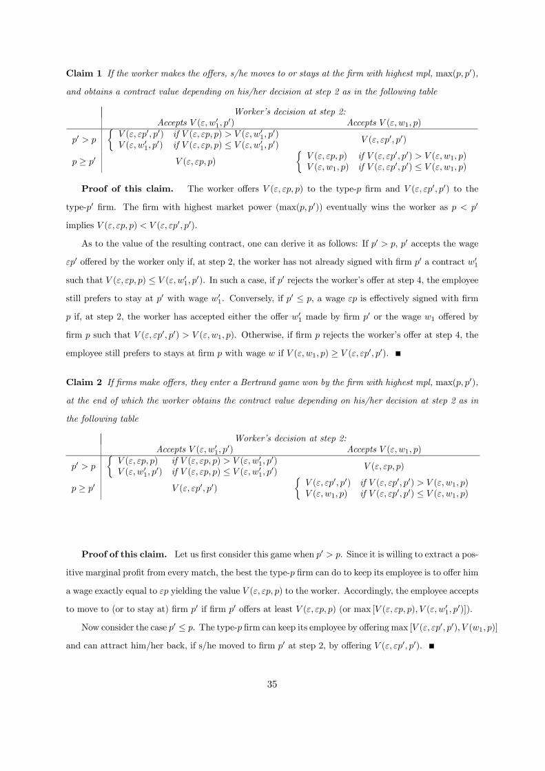
Claim 1 If the worker makes the offers, s/he moves to or stays at the firm with highest mpl, max(p, p0),

and obtains a contract value depending on his/her decision at step 2 as in the following table

Worker’s decision at step 2:Accepts V (ε, w01, p0) Accepts V (ε, w1, p)

p0 > p½V (ε, εp0, p0) if V (ε, εp, p) > V (ε, w01, p0)V (ε, w01, p0) if V (ε, εp, p) ≤ V (ε, w01, p0) V (ε, εp0, p0)

p ≥ p0 V (ε, εp, p)

½V (ε, εp, p) if V (ε, εp0, p0) > V (ε, w1, p)V (ε, w1, p) if V (ε, εp0, p0) ≤ V (ε, w1, p)

Proof of this claim. The worker offers V (ε, εp, p) to the type-p firm and V (ε, εp0, p0) to the

type-p0 firm. The firm with highest market power (max(p, p0)) eventually wins the worker as p < p0

implies V (ε, εp, p) < V (ε, εp0, p0).

As to the value of the resulting contract, one can derive it as follows: If p0 > p, p0 accepts the wage

εp0 offered by the worker only if, at step 2, the worker has not already signed with firm p0 a contract w01

such that V (ε, εp, p) ≤ V (ε, w01, p0). In such a case, if p0 rejects the worker’s offer at step 4, the employeestill prefers to stay at p0 with wage w01. Conversely, if p

0 ≤ p, a wage εp is effectively signed with firmp if, at step 2, the worker has accepted either the offer w01 made by firm p0 or the wage w1 offered by

firm p such that V (ε, εp0, p0) > V (ε, w1, p). Otherwise, if firm p rejects the worker’s offer at step 4, the

employee still prefers to stays at firm p with wage w if V (ε, w1, p) ≥ V (ε, εp0, p0).

Claim 2 If firms make offers, they enter a Bertrand game won by the firm with highest mpl, max(p, p0),

at the end of which the worker obtains the contract value depending on his/her decision at step 2 as in

the following table

Worker’s decision at step 2:Accepts V (ε, w01, p0) Accepts V (ε, w1, p)

p0 > p½V (ε, εp, p) if V (ε, εp, p) > V (ε, w01, p0)V (ε, w01, p0) if V (ε, εp, p) ≤ V (ε, w01, p0) V (ε, εp, p)

p ≥ p0 V (ε, εp0, p0)½V (ε, εp0, p0) if V (ε, εp0, p0) > V (ε, w1, p)V (ε, w1, p) if V (ε, εp0, p0) ≤ V (ε, w1, p)

Proof of this claim. Let us first consider this game when p0 > p. Since it is willing to extract a pos-

itive marginal profit from every match, the best the type-p firm can do to keep its employee is to offer him

a wage exactly equal to εp yielding the value V (ε, εp, p) to the worker. Accordingly, the employee accepts

to move to (or to stay at) firm p0 if firm p0 offers at least V (ε, εp, p) (or max [V (ε, εp, p), V (ε, w01, p0)]).

Now consider the case p0 ≤ p. The type-p firm can keep its employee by offeringmax [V (ε, εp0, p0), V (w1, p)]and can attract him/her back, if s/he moved to firm p0 at step 2, by offering V (ε, εp0, p0).

35

Step 2. At step 2, the worker chooses the offer that yields the highest expected utility in the continuing

negotiation game. If s/he refuses both offers, s/he gets the value V (ε, w, p) of the pre-existing contract

with the incumbent firm. Otherwise s/he gets the values EV as in the following table:

Worker’s decision at step 2:Accepts V (ε, w01, p0) Accepts V (ε, w1, p)

p0 > p

EV = βV (ε, εp0, p0) + (1− β)V (ε, εp, p)

if V (ε, εp, p) > V (ε, w01, p0)

EV = V (ε, w01, p0)

if V (ε, εp, p) ≤ V (ε, w01, p0)

EV = βV (ε, εp0, p0) + (1− β)V (ε, εp, p)

p ≥ p0 EV = βV (ε, εp, p) + (1− β)V (ε, εp0, p0)

EV = βV (ε, εp, p) + (1− β)V (ε, εp0, p0)

if V (ε, εp0, p0) > V (ε, w1, p)

EV = V (ε, w1, p)if V (ε, εp0, p0) ≤ V (ε, w1, p)

Step 1. At step 1, employers make simultaneous offers. Both employers offer the lowest possible wage

that attracts the worker (and still yields nonnegative profits).

Claim 3 At step 1, the firm with highest mpl, max(p, p0), makes an offer immediately accepted provided

that it improves the worker’s value. This offer defines a wage φ(ε, p, p0) which solves:

V (ε,φ(ε, p, p0), p0) = βV (ε, εp0, p0) + (1− β)V (ε, εp, p) if p0 > pV (ε,φ(ε, p0, p), p) = βV (ε, εp, p) + (1− β)V (ε, εp0, p0) if p ≥ p0 (A2)

Proof of this claim.

• If p0 > p, the preceding table of expected outcomes implies that the worker can get at least

EV = βV (ε, εp0, p0)+ (1−β)V (ε, εp, p) in the continuing negotiation game by accepting any offer

made by the type-p firm. In order to avoid a waste of time in unnecessary negotiation, firm p0

offers a wage w01 = φ(ε, p, p0), that the worker accepts at step 2 and that solves:

V (ε,φ(ε, p, p0), p0) = βV (ε, εp0, p0) + (1− β)V (ε, εp, p).

Firm p cannot bid this wage that is bigger than εp.

• If p0 ≤ p, the worker can get at least EV = βV (ε, εp, p)+(1−β)V (ε, εp0, p0) by accepting any offermade by the type-p0 firm. In order to avoid a waste of time, firm p offers a wage w1 = φ(ε, p0, p),

that the worker accepts at step 2 and that solves:

V (ε,φ(ε, p0, p0), p) = βV (ε, εp, p) + (1− β)V (ε, εp0, p0).

Firm p0 cannot bid this wage that is bigger than εp0.

36

This completes the characterization of the subgame perfect equilibrium of our bargaining game. It is

worth introducing some extra notation at this point (for later use): we see that the minimal value of p0

for which “something happens” (i.e. either causing a wage increase or an employer change) is q(ε, w, p)

such that

V (ε, w, p) = βV (ε, εp, p) + (1− β)V (ε, εq(ε, w, p), q(ε, w, p)). (A3)

Note that

V (ε, εq(ε, w, p), q(ε, w, p)) = V (ε, w, p)− β

1− β[V (ε, εp, p)− V (ε, w, p)]

< V (ε, w, p)

whenever w < p.

A.2 Equilibrium wage determination

Here we derive the precise closed-form of equilibrium wages φ0(ε, p) and φ (ε, p, p0) defined in equations (1)

and (2) respectively. The first step is to derive the value functions V0 (·) and V (·). Time is discountedat rate ρ. Since offers accrue to unemployed workers at rate λ0, V0 (ε) solves the following Bellman

equation:

(ρ+ λ0) V0 (ε) = εb+ λ0EF {max [V (ε,φ0(ε,X),X), V0]} , (A4)

where EF is the expectation operator with respect to a variable X, which has distribution F . Using the

definition (A1) to replace V (ε,φ0 (ε, p) , p) by βV (ε, p, p) + (1− β)V0(ε) in the latter equation, we then

show that:

ρV0 (ε) = εb+ λ0EF {max (β [V (ε,φ0(ε,X),X)− V0(ε)] , 0)} . (A5)

We thus find that an unemployed worker’s expected lifetime utility depends on his personal ability ε

through the amount of output he produces when engaged in home production, εb, but also on labor

market parameters such as the distribution of jobs and his bargaining power β.

Now turning to employed workers, consider a type-ε worker employed at a type-p firm. Since layoffs

occur at rates δ, we may now write the Bellman equation solved by the value function V (ε, w, p):

£ρ+ δ + λ1F (q (ε, w, p))

¤V (ε, w, p) = w

+ λ1 [F (p)− F (q (ε, w, p))] EF {V (ε,φ (ε,X, p) ,X) |q (ε, w, p) ≤ X ≤ p}

+ λ1F (p)EF {V (ε,φ (ε, p,X) ,X) |p ≤ X}+ δV0 (ε) . (A6)

37

Let us denote by pmax the upper support of p. Equations (A3) and (A6), together with the bargaining

rule (A2) allow us to rewrite (A6) as follows:

£ρ+ δ + λ1F (q (ε, w, p))

¤V (ε, w, p) = w + δV0 (ε)+

λ1

Z p

q(ε,w,p)

[(1− β)V (ε, εx, x) + βV (ε, εp, p)] dF (x)+

λ1

Z pmax

p

[(1− β)V (ε, εp, p) + βV (ε, εx, x)] dF (x). (A7)

Imposing w = εp in (A7), taking the derivative, and noticing that the definition (A3) of q(ε, w, p) implies

that q(ε, εp, p) = p, one gets:dV (ε, εp, p)

dp=

ε

ρ+ δ + λ1βF (p). (A8)

Then, integrating by parts in equation (A7):

(ρ+ δ)V (ε, w, p) = w + δV0(ε) + βλ1ε

Z pmax

p

F (x)

ρ+ δ + λ1βF (x)dx

+ (1− β)λ1ε

Z p

q(ε,w,p)

F (x)

ρ+ δ + λ1βF (x)dx. (A9)

Again imposing w = εp, the last equation in turn implies that

(ρ+ δ)V (ε, εp, p) = εp+ δV0 (ε) + βλ1ε

Z pmax

p

F (x)

ρ+ δ + λ1βF (x)dx. (A10)

Noticing that q (ε,φ (ε, p0, p) , p) = p0, an expression of V (ε,φ (ε, p0, p) , p) can be obtained from (A9):

(ρ+ δ)V (ε,φ (ε, p0, p) , p) = φ (ε, p0, p) + δV0(ε) + βλ1ε

Z pmax

p

F (x)

ρ+ δ + λ1βF (x)dx

+ (1− β)λ1ε

Z p

p0

F (x)

ρ+ δ + λ1βF (x)dx. (A11)

But, following the bargaining rule (A2), (ρ+ δ)V (ε,φ (ε, p0, p) , p) should also equal

(ρ+ δ) [βV (ε, εp, p) + (1− β)V (ε, εp0, p0)]

which, using (A10), writes as:

βεp+ (1− β) εp0 + δV0(ε) + β2λ1ε

Z pmax

p

F (x)

ρ+ δ + λ1βF (x)dx+ β(1− β)λ1ε

Z pmax

p0

F (x)

ρ+ δ + λ1βF (x)dx.

Equating this expression with the right hand side of equation (A11), one gets the following expression

for the wage φ (ε, p0, p):

φ (ε, p0, p) = βεp+ (1− β)εp0 − (1− β)2λ1

Z p

p0

εF (x)

ρ+ δ + λ1βF (x)dx. (A12)

38

The lower support of the distribution of marginal productivities, pmin, cannot fall short of the value

pinf such that V (ε, εpinf , pinf) = V0(ε). Using the definitions (A5), of V0(ε), and (A9), of V (ε, w, p), this

identity yields:

pinf = b+ β(λ0 − λ1)

Z pmax

pinf

F (x)

ρ+ δ + λ1βF (x)dx. (A13)

(Note that the value of pinf is independent of ε. This result holds true for any homogeneous specification

of the utility function.) Finally, as the bargaining outcome implies (A12), the identity V (ε, εpinf , pinf) =

V0(ε) implies the following alternative definition of φ0 (ε, p):

φ0(ε, p) = φ(ε, pinf , p) = βεp+ (1− β)εpinf − (1− β)2λ1

Z p

pinf

εF (x)

ρ+ δ + λ1βF (x)dx. (A14)

A.3 Equilibrium wage distributions

The G (w|ε, p) ` (ε, p) (1 − u)M workers of type ε, employed at firms of type p, and paid less than

w ∈ [φ0(ε, p), εp] leave this category either because they are laid off (rate δ), or because they receive anoffer from a firm with mpl p ≥ q (ε, w, p) which grants them a wage increase or induces them to leave

their current firm (rate λ1F [q (ε, w, p)]). On the inflow side, workers entering the category (ability ε,

wage ≤ w, mpl p) come from two distinct sources. Either they are hired away from a firm less productivethan q (ε, w, p), or they come from unemployment. The steady-state equality between flows into and out

of the stocks G (w|ε, p) ` (ε, p) thus takes the form:

©δ + λ1F [q (ε, w, p)]

ªG (w|ε, p) ` (ε, p) (1− u)M

=

(λ0uM h (ε) + λ1(1− u)M

Z q(ε,w,p)

pmin

`(ε, x)dx

)f(p)

=

(δh (ε) + λ1

Z q(ε,w,p)

pmin

`(ε, x)dx

)(1− u)Mf(p), (A15)

since λ0u = δ(1−u). Applying this identity for w = εp (which has the property that G (εp|ε, p) = 1 andq (ε, εp, p) = p), we get:

©δ + λ1F (p)

ª` (ε, p) =

½δh (ε) + λ1

Z p

pmin

`(ε, x)dx

¾f(p),

which solves as

` (ε, p) =1 + κ1£

1 + κ1F (p)¤2h (ε) f (p) .

This shows that ` (ε, p) has the form h (ε) ` (p) (absence of sorting), and gives the expression of ` (p).

Hence the equations (10) and (11). Equation (10) can be integrated between pmin and p to obtain (9).

Substituting (9), (10) and (11) into (A15) finally yields equation (12).

39

A.4 Derivation of E[T (w)|p] for any integrable function T (w)

The lowest paid type-ε worker in a type-p firm is one that has just been hired, therefore earning φ0 (ε, p) =

φ(ε, pinf , p), while the highest-paid type-ε worker in that firm earns his marginal productivity εp. Thus,

the support of the within-firm earnings distribution of type ε workers for any type-p firm belongs to

the interval [pinf , p]. Noticing that eG(q|p) = G (φ(ε, q, p)|ε, p) has a mass point at pinf and is otherwisecontinuous over the interval [pmin, p], we can readily show that for any integrable function T (w),

E [T (w)|p] =Z εmax

εmin

ÃZ εp

φ(ε,pmin,p)

T (w) G (dw|ε, p) + T (φ0 (ε, p)) G (φ0 (ε, p) |ε, p)!h(ε)dε

=£1 + κ1F (p)

¤2 ( 1

(1 + κ1)2

Z εmax

εmin

T (φ0 (ε, p))h(ε)dε

+

Z p

pmin

·Z εmax

εmin

T (φ (ε, q, p))h(ε)dε

¸2κ1f(q)£

1 + κ1F (q)¤3 dq

)

=

Z εmax

εmin

T (εp)h(ε)dε+

£1 + κ1F (p)

¤2[1 + κ1]

2

Z εmax

εmin

[T (φ0 (ε, p))− T (φ (ε, pmin, p))]h(ε)dε

− £1 + κ1F (p)¤2 Z p

pmin

·Z εmax

εmin

T 0 (φ (ε, q, p)) εh(ε)dε¸

(1− β)£1 + (1− σ)κ1F (q)

¤£1 + (1− σ)κ1βF (q)

¤ £1 + κ1F (q)

¤2 dq. (A16)

The first equality follows from the definition of G (w|ε, p) as

G (w|ε, p) =£1 + κ1F (p)

¤2£1 + κ1F (q(ε, w, p))

¤2yielding

G0(w|ε, p) = £1 + κ1F (p)¤2h(ε)

2κ1f(q)£1 + κ1F (q)

¤3 · ∂q(ε, w, p)∂wdw.

The second equality is obtained with an integration by parts, deriving the partial derivative of φ (ε, q, p)

with respect to q from (A12) as

∂φ (ε, q, p)

∂q= (1− β)ε · 1 + (1− σ)κ1F (q)

1 + (1− σ)κ1βF (q).

References

[1] Abowd, J., F. Kramarz and D. Margolis (1999), “High wage workers and high wage firms”, Econo-

metrica, 67, 251-335.

[2] Abowd, J.A. and T. Lemieux (1993), “The Effects of Product Market Competition on Collective

Bargaining Agreements: The Case of Foreign Competition in Canada,” Quarterly Journal of Eco-

nomics, 108(4), 983-1014.

40

[3] Arellano, M. and S. R. Bond (1991), “Some Tests of Specification for Panel Data: Monte Carlo

Evidence and an Application to Employment Equations,” Review of Economic Studies, 58, 277-97.

[4] Arellano, M. and O. Bover (1995), “Another Look at the Instrumental-Variable Estimation of

Error-Components Models,” Journal of Econometrics, 68, 29-52.

[5] Binmore, K., A. Rubinstein and A. Wolinsky (1986), “The Nash Solution in Economic Modelling,”

Rand Journal of Economics, 17, 176-88.

[6] Blanchflower, D., A. Oswald and P. Sanfrey (1996), “Wages, Profits and Rent Sharing,” Quarterly

Journal of Economics, 111(1), 227-251.

[7] Burdett, K. and D. T. Mortensen (1998), “Wage Differentials, Employer Size and Unemployment,”

International Economic Review, 39, 257-73.

[8] Cahuc, P. and E. Wasmer (2001), “Does intrafirm bargaining matter in the large firm’s matching

model?,” Macroeconomic Dynamics, 5, 742-747.

[9] Chamberlain, G. (1992), “Comment: Sequential Moment Restrictions in Panel Data,” Journal of

Business & Economic Statistics, 10(1), 275-281.

[10] Christensen, B. J., R. Lentz, D. T. Mortensen, G. R. Neumann and A. Werwatz (2001) “On the

Job Search and the Wage Distribution,” Northwestern University Working Paper.

[11] Crépon, B. and R. Desplatz (2002), “Evaluation of the Effects of Payroll Tax Subsidies for LowWage

Workers,” CREST-INSEE, available from www.crest.fr/pageperso/dr/crepon/payrolltax.pdf.

A simplified version was published in French in 2002 in Economie et Statistiques as “Evaluation

des effets des dispositifs d’allègement de charges sur les bas salaires”.

[12] Dey, M. S. and C. J. Flinn (2000), “An Equilibrium Model of Health Insurance Provision and Wage

Determination,” mimeo, University of Chicago and New York University.

[13] Eckstein, Z. and K. I. Wolpin (1995), “Duration to First Job and the Return to Schooling: Estimates

from a Search-Matching Model,” The Review of Economic Studies, 62, 263-286.

[14] Hosios, D. (1990), “On the Efficiency of Matching and Related Models of Search and Unemploy-

ment,” Review of Economic Studies, 57, 279-298.

[15] Kramarz, F. (2002), “Bargaining and International Trade,” mimeo, CREST-INSEE.

[16] MacLeod, W. and J. Malcomson (1993), “Investment, Holdup, and the Form of Market Contracts,”

American Economic Review, 83, 811-37.

41

[17] Malcomson, J. (1999), “Individual Employment Contracts,” in Ashenfelter, O. and Card, D. (eds),

Handbook of Labor Economics, vol 3, Chapter 35, 2291-2372, Elsevier Science.

[18] Margolis, D. N. and K.G. Salvanes (2001) “Do Firms Really Share Rents With Their Workers,”

mimeo, CREST-INSEE.

[19] Mortensen, D.T. (1990), “Equilibrium wage distributions: a synthesis,” in J. Hartog et al., editor,

Panel data and labour market studies, North-Holland, Amsterdam.

[20] Mortensen, D. (2002), “Wage Dispersion: Why Are Similar Workers Paid Differently?,” mimeo,

Northwestern University.

[21] Mortensen, D. and C. A. Pissarides (1999), “Job Reallocation, Employment Fluctuations and Un-

employment,” in Woodford, M. and Taylor, J. (eds), Handbook of Macroeconomics, Elsevier Science

Publisher, vol 1B, Chapter 18, 1171-1228.

[22] Osborne, M. and A. Rubinstein (1990), Bargaining and Markets, San Diego: Academic Press.

[23] Pissarides, C. A. (2000), Equilibrium unemployment theory, 2nd edition, Cambridge, MIT Press.

[24] Postel-Vinay, F. and J.-M. Robin (2002a), “The Distribution of Earnings in an Equilibrium Search

Model with State-Dependent Offers and Counter-Offers,” International Economic Review, 43(4),

1-26.

[25] Postel-Vinay, F. and J.-M. Robin (2002b), “Equilibrium Wage Dispersion with

Worker and Employer Heterogeneity,” INRA-LEA WP. No 00-08. (Available from

www.inra.fr/Internet/Departements/ESR/UR/lea/DocumentW.htm), forthcoming Econo-

metrica.

[26] Stole, L.A. and J. Zwiebel (1996), “Organizational Design and Technology Choice under Intrafirm

Bargaining”. American Economic Review, 86(1), 195-222.

[27] van den Berg, G. J. and G. Ridder (2000), “A Cross-Country Comparison of Labor Market Fric-

tions,” mimeo.

[28] Van Reenen, J. (1996), “The Creation and Capture of Economic Rents: Wages and Innovations in

a Panel of UK Companies,” Quarterly Journal of Economics, 111(1), 195-226.

[29] Wolinsky, A. (2000), “A Theory of the Firm with Non-Binding Employment Contracts,” Econo-

metrica, 68(4), 875-910.

42

WDEOH4=Vdpsoh

ghvfuls

wlyhvwd

wlvwlfv

Lqgxvwu|

Qr1ri

�up

v

Qr1ri

xqvnloohg

zrunhuv/

+(riwrwdo,

Qr1ri

vnloohg

zrunhuv/

+(riwrwdo,

Phdq

�up

vl}h

Phdq

dqqxdo

y1d1shu

fdslwd

Phdq

vkduh

ri

oderu

lqy1d1

Phdqdqqxdo

frpshqvdwlr

qfrvwv

Pdqxidfwxulqj

Lqwhup

hgldwh

jrrgv

:/353

4/453/:::

+::19(,

656/45:

+5517(,

Xqvn1=

641<

Vnloohg

=<15

76/;87

:318(

Xqvn1=

57/39:

Vnloohg

=7;/5;;

Udwlr

=513

Lqyhvwp

hqwjrrgv

6/<;3

96:/7;<

+:319(,

598/765

+5<17(,

Xqvn1=

65

Vnloohg

=4616

75/785

:71:(

Xqvn1=

56/;;3

Vnloohg

=77/<9;

Udwlr

=41<

Frqvxpswlr

qjrrgv

</996

4/687/7<7

+:81;(,

766/7:<

+5715(,

Xqvn1=

5;

Vnloohg

=<

74/9:5

:315(

Xqvn1=

54/865

Vnloohg

=73/84:

Udwlr

=41<

Hohfwulfd

o)

hohfwurqlf

htxlsphqw

4/854

568/93:

+9519(,

473/:<<

+6:17(,

Xqvn1=

64

Vnloohg

=4;18

76/686

:81:(

Xqvn1=

59/988

Vnloohg

=7</<<7

Udwlr

=41<

Frqvwuxfwlrq

45/394

<95/:93

+;41;(,

546/;<;

+4;15(,

Xqvn1=

49

Vnloohg

=618

69/643

9<17(

Xqvn1=

4</:<:

Vnloohg

=68/<55

Udwlr

=41;

Wudqvsruwdwlrq

4/<:9

64</6<4

+;41;(,

:4/35;

+4;15(,

Xqvn1=

6516

Vnloohg

=:15

74/<54

:319(

Xqvn1=

54/<<9

Vnloohg

=6;/:67

Udwlr

=41;

Wudgh

Zkrohvd

oh/irrg

6/4:9

536/<:8

+:31<(,

;6/:43

+5<14(,

Xqvn1=

451;

Vnloohg

=816

7:/59<

9819(

Xqvn1=

54/9;9

Vnloohg

=76/363

Udwlr

=513

Zkrohvd

oh/qrqirrg

</4<6

885/:<8

+8:14(,

748/:;7

+751<(,

Xqvn1=

45

Vnloohg

=<

7;/;73

:513(

Xqvn1=

55/88:

Vnloohg

=76/:3;

Udwlr

=41<

Uhwd

lo/irrg

6/9;<

699/;68

+;61<(,

:3/8;;

+4914(,

Xqvn1

4<1<

Vnloohg

=61;

66/837

9916(

Xqvn1=

4:/589

Vnloohg

=65/347

Udwlr

=41<

Uhwd

lo/qrqirrg

;/956

59;/395

+:51<(,

<</:5<

+5:14(,

Xqvn1=

915

Vnloohg

=516

6;/83;

:313(

Xqvn1=

4</657

Vnloohg

=67/3;:

Udwlr

=41;

Vhuylfhv

Dxwrpreloh

uhsdlu)

wudgh

9/3<<

669/355

+::16(,

<;/7;5

+551:(,

Xqvn1=

44

Vnloohg

=615

6</3<9

:31:(

Xqvn1=

54/55:

Vnloohg

=68/84<

Udwlr

=419

Krwhov

)uhvwd

xudqwv

6/;4<

499/:48

+:914(,

85/639

+561<(,

Xqvn1=

;1:

Vnloohg

=51:

68/8;5

9916(

Xqvn1=

4:/<:<

Vnloohg

=59/75<

Udwlr

=418

Shuvr

qdovhuy

lfhv7/<4;

87</995

+:617(,

4<</4:<

+5919(,

Xqvn1=

5517

Vnloohg

=;14

68/476

:316(

Xqvn1=

4;/395

Vnloohg

=63/977

Udwlr

=41:

TABLE 2: Production Function Estimates1

Industry ξ α

ManufacturingIntermediate goods 0.99

(0.02)11.85(0.18)

Investment goods 0.94(0.02)

1.66(0.14)

Consumption goods 1.03(0.02)

1.71(0.12)

Electrical & electronic equipment 0.96(0.03)

1.59(0.19)

Construction 0.95(0.02)

1.42(0.10)

Transportation 0.90(0.03)

1.55(0.23)

TradeWholesale, food 0.95

(0.03)1.65(0.27)

Wholesale, nonfood 0.96(0.02)

1.66(0.09)

Retail, food 0.94(0.02)

1.33(0.19)

Retail, nonfood 0.95(0.02)

1.48(0.10)

ServicesAutomobile repair & trade 0.99

(0.02)1.17(0.11)

Hotels & restaurants 0.89(0.04)

1.16(0.13)

Personal services 1.00(0.03)

1.71(0.15)

Note: 1Standard errors in parentheses.

44

TABLE 3: Transition Parameter Estimates1

Industry Labor type λ1 1/λ1 δ 1/δ κ1 =λ1δ

Manufacturing Unskilled 0.058(0.004)2

17.0 0.043(0.001)

22.9 1.34(0.11)

Skilled 0.086(0.010)

11.5 0.027(0.001)

36.1 3.13(0.52)

Construction Unskilled 0.188(0.018)

5.3 0.068(0.003)

20.6 2.75(0.35)

Skilled 0.195(0.048)

5.1 0.048(0.005)

14.6 4.02(1.30)

Transportation Unskilled 0.142(0.019)

7.04 0.043(0.003)

23.3 3.30(0.62)

Skilled 0.065(0.022)

15.4 0.028(0.005)

35.7 2.34(1.06)

Trade Unskilled 0.115(0.009)

8.6 0.063(0.002)

15.8 1.83(0.18)

Skilled 0.231(0.032)

4.3 0.043(0.002)

22.8 5.28(0.98)

Services Unskilled 0.307(0.019)

3.3 0.099(0.002)

10.0 3.08(0.25)

Skilled 0.257(0.031)

3.9 0.049(0.002)

20.3 5.23(0.84)

Notes: 1Per annum.2Standard errors in parentheses.

45

TABLE 4: Bargaining Power Estimates1

Industry Unskilled SkilledManufacturingIntermediate goods 0.00

(0.000)20.01(0.005)

Investment goods 0.10(0.004)

0.26(0.008)

Consumption goods 0.00(0.000)

0.08(0.005)

Electrical & electronic equipment 0.14(0.004)

0.36(0.007)

Construction 0.00(0.000)

0.46(0.008)

Transportation 0.08(0.006)

0.49(0.011)

TradeWholesale, food 0.00

(0.000)0.12(0.007)

Wholesale, nonfood 0.01(0.003)

0.15(0.004)

Retail, food 0.00(0.000)

0.69(0.015)

Retail, nonfood 0.00(0.000)

0.21(0.007)

ServicesAutomobile repair & trade 0.00

(0.000)0.83(0.014)

Hotels & restaurants 0.00(0.000)

0.60(0.014)

Personal services 0.00(0.000)

0.00(0.003)

Notes: 1Estimates obtained with ρ = 0.15.2Standard errors in parentheses.

46

WDEOH8=Phdqzrunhu

vkduh

ripdwfk

uhqwv�

Lqgxvwu|

revhuy

hg=e�f

suhg

lfwhg=ee�f

vkduh

riee�fgxh

wrehwz

hhq0�up

frpshwlwlr

q

Xqvnloohg

Vnlooh

gXqvnloohg

Vnloohg

Xqvnloohg

Vnloohg

Pdqxidfwxulqj

Lqwhup

hgldwh

jrrgv

3=58

3=6;

3=5:

3=73

433(

<:=8(

Lqyhvwp

hqwjrrgv

3=6:

3=8;

3=6;

3=94

:<=<(

:4=;(

Frqvxpswlr

qjrrgv

3=59

3=77

3=5<

3=7:

433(

;<=4(

Hohfwulf

do)hoh

fwurqlfhtxlsphqw

3=6;

3=96

3=6<

3=97

9<=5(

95=:(

Frqvwuxfwlr

q3=43

3=:7

3=63

3=:6

<;=8(

93=5(

Wudqvsruwdwlrq

3=79

3=:6

3=7<

3=:8

<3=6(

8:=4(

Wudgh

Zkrohvd

oh/irrg

3=59

3=7;

3=5<

3=83

433(

;6=7(

Zkrohvd

oh/qrqirrg

3=63

3=85

3=68

3=89

<:=<(

:<=;(

Uhwd

lo/irrg

3=4;

3=;8

3=5:

3=;8

<<=<(

:<=;(

Uhwd

lo/qrqirrg

3=58

3=89

3=64

3=93

433(

:9=8(

Vhuylfhv

Dxwrpreloh

uhsdlu)wud

gh

3=43

3=<7

3=54

3=<8

433(

85=5(

Krwhov

)uhvwd

xudqwv

3=5;

3=;5

3=65

3=;7

433(

89=6(

Shuvr

qdovhuylfhv

3=5<

3=6:

3=65

3=78

433(

433(

Qrwh=�Hvwlp

dwhv

rewdlqhg

zlwk

�@3=481

WDEOH9=Frpsdudwly

hVwdwlf

vrqPhdqZdjhv

Lqgxvwu|

Orjphdq

zdjh

E*?��

Suhglfwhg

orjphdq

zdjh

�*? e� �

Suhglfwlr

q

huur

u�*? e�

3*?� �

Y*? e�Yq

Y*? e�YV�

Y*? e�Yq

�����V4'f

Y*? e�YV� �����

V4'f

Pdqxidfwxulqj

Lqwhup

hgldwh

jrrgv

Xqvn1=

7167

Vnlooh

g=

8139

Xqvn1=

7169

Vnlooh

g=

813<

Xqvn1=

513(

Vnlooh

g=

51<(

Xqvn1=

3195

Vnlooh

g=

3186

Xqvn1=

3143

Vnlooh

g=

3138

Xqvn1=

31::

Vnlooh

g=

31:8

Xqvn1=

316:

Vnloohg

=316:

Lqyhvwp

hqwjrrgv

Xqvn1=

7169

Vnlooh

g=

71<<

Xqvn1=

716:

Vnlooh

g=

8138

Xqvn1=

31<(

Vnlooh

g=

913(

Xqvn1=

3184

Vnlooh

g=

3169

Xqvn1=

3143

Vnlooh

g=

3138

Xqvn1=

3199

Vnlooh

g=

3194

Xqvn1=

3165

Vnloohg

=315;

Frqvxpswlr

qjrrgv

Xqvn1=

7157

Vnlooh

g=

8133

Xqvn1=

7158

Vnlooh

g=

71<<

Xqvn1=

31:(

Vnlooh

g=

3��fI

Xqvn1=

31:6

Vnlooh

g=

3189

Xqvn1=

3146

Vnlooh

g=

3139

Xqvn1=

31<5

Vnlooh

g=

31;:

Xqvn1=

3178

Vnloohg

=3175

Hohfwulfd

o)

hohfwur

qlf

htxlsphqw

Xqvn1=

71;3

Vnlooh

g=

8173

Xqvn1=

71;:

Vnlooh

g=

8183

Xqvn1=

;13(

Vnlooh

g=

4318(

Xqvn1=

3186

Vnlooh

g=

3167

Xqvn1=

3143

Vnlooh

g=

3138

Xqvn1=

31:5

Vnlooh

g=

3194

Xqvn1=

3168

Vnloohg

=315:

Frqvwuxfwlrq

Xqvn1=

7164

Vnlooh

g=

8133

Xqvn1=

7177

Vnlooh

g=

71<;

Xqvn1=

461<(

Vnlooh

g=

3���I

Xqvn1=

3177

Vnlooh

g=

3157

Xqvn1=

3136

Vnlooh

g=

3136

Xqvn1=

3189

Vnlooh

g=

3176

Xqvn1=

315:

Vnloohg

=314:

Wudqvsruwdwlrq

Xqvn1=

7185

Vnlooh

g=

8145

Xqvn1=

7184

Vnlooh

g=

8148

Xqvn1=

3f�bI

Vnlooh

g=

51:(

Xqvn1=

317<

Vnlooh

g=

316:

Xqvn1=

3137

Vnlooh

g=

3139

Xqvn1=

31:3

Vnlooh

g=

3194

Xqvn1=

3166

Vnloohg

=3159

Wudgh

Zkrohvdoh/irrg

Xqvn1=

7159

Vnlooh

g=

71<8

Xqvn1=

7164

Vnlooh

g=

71<<

Xqvn1=

813(

Vnlooh

g=

71:(

Xqvn1=

31:5

Vnlooh

g=

3185

Xqvn1=

313;

Vnlooh

g=

3136

Xqvn1=

31;;

Vnlooh

g=

31:9

Xqvn1=

3174

Vnloohg

=3169

Zkrohvdoh/qrqirrg

Xqvn1=

715<

Vnlooh

g=

71<:

Xqvn1=

715;

Vnlooh

g=

71<:

Xqvn1=

3��2I

Vnlooh

g=

316(

Xqvn1=

319;

Vnlooh

g=

317;

Xqvn1=

313;

Vnlooh

g=

3136

Xqvn1=

31:<

Vnlooh

g=

31:3

Xqvn1=

316:

Vnloohg

=3165

Uhwdlo/

irrg

Xqvn1=

61<:

Vnlooh

g=

71:<

Xqvn1=

7148

Vnlooh

g=

71:4

Xqvn1=

4<1;(

Vnlooh

g=

3.��I

Xqvn1=

3185

Vnlooh

g=

3154

Xqvn1=

3139

Vnlooh

g=

3135

Xqvn1=

319<

Vnlooh

g=

3179

Xqvn1=

3167

Vnloohg

=3149

Uhwdlo/

qrqirrg

Xqvn1=

7146

Vnlooh

g=

71;6

Xqvn1=

714:

Vnlooh

g=

71:9

Xqvn1=

7143(

Vnlooh

g=

3S�.I

Xqvn1=

3199

Vnlooh

g=

3174

Xqvn1=

313;

Vnlooh

g=

3136

Xqvn1=

31;3

Vnlooh

g=

3198

Xqvn1=

316;

Vnloohg

=315<

Vhuylfhv

Dxwrpreloh

uhsdlu)

wudgh

Xqvn1=

61;9

Vnlooh

g=

7186

Xqvn1=

7133

Vnlooh

g=

7178

Xqvn1=

4817(

Vnlooh

g=

3.�2I

Xqvn1=

3196

Vnlooh

g=

314;

Xqvn1=

3136

Vnlooh

g=

3135

Xqvn1=

319<

Vnlooh

g=

3177

Xqvn1=

3164

Vnloohg

=3147

Krwhov)

uhvwd

xudqwv

Xqvn1=

6198

Vnlooh

g=

7159

Xqvn1=

619<

Vnlooh

g=

714:

Xqvn1=

61<(

Vnlooh

g=

3b��I

Xqvn1=

31:;

Vnlooh

g=

315:

Xqvn1=

3137

Vnlooh

g=

3136

Xqvn1=

31:;

Vnlooh

g=

3188

Xqvn1=

3167

Vnloohg

=3154

Shuvr

qdovhuylfh

vXqvn1=

7135

Vnlooh

g=

719;

Xqvn1=

7135

Vnlooh

g=

719<

Xqvn1=

3f�.I

Vnlooh

g=

418(

Xqvn1=

31:5

Vnlooh

g=

3189

Xqvn1=

3137

Vnlooh

g=

3136

Xqvn1=

31:4

Vnlooh

g=

31:7

Xqvn1=

3163

Vnloohg

=3169

WDEOH:=Lqwhulq

gxvwu|

zdjhgl�huhq

wldov�

Frxqwhuid

fwxdoDqdo|vlv

Lqgxvwu|

Suhg

lfwhgorjphdqzdjh

Frxqwhuid

fwxdo*?�

zkhq

111

�*? e� �

R'Roes�

k'koes�

q'qoes�

V�'V�co

es�

R'Roes�

k'koes�

q'qoes�

Pdqxidfwxulqj

Lqwhup

hgldwh

jrrgv

Xqvn1=

7169

+uhi1,Vnloohg

=813<

+uhi1,Xqvn1=

�+uhi1,

Vnloohg

=�

+uhi1,Xqvn1=

�+uhi1,

Vnloohg

=�

+uhi1,Xqvn1=

�+uhi1,

Vnloohg

=�

+uhi1,Xqvn1=

�+uhi1,

Vnloohg

=�

+uhi1,

Lqyhvwp

hqwjrrgv

Xqvn1=

716:

Ef�bI�

Vnloohg

=8138

E3e�eI�

Xqvn1=

7175

ED�bI�

Vnloohg

=8154

E���bI�

Xqvn1=

7165

E3e�eI�

Vnloohg

=71<8

E3�e��I�

Xqvn1=

��

Vnloohg

=�

�Xqvn1=

7169

EfI�

Vnloohg

=813<

EfI�

Frqvxpswlr

qjrrgv

Xqvn1=

7158

E3�f�HI�

Vnloohg

=71<<

E3�f�eI�

Xqvn1=

7169

EfI�

Vnloohg

=8145

E��2I�

Xqvn1=

7158

E3�f�HI�

Vnloohg

=71<8

E3�e�fI�

Xqvn1=

��

Vnloohg

=�

�Xqvn1=

7169

EfI�

Vnloohg

=813<

EfI�

Hohfwulfd

o)

hohfwurqlf

htxlsphqw

Xqvn1=

71;:

ED���I�

Vnloohg

=8183

Ee���I�

Xqvn1=

7177

EH��I�

Vnloohg

=8158

E�S�fI�

Xqvn1=

71:<

Ee���I�

Vnloohg

=816:

E2.�DI�

Xqvn1=

��

Vnloohg

=�

�Xqvn1=

7169

EfI�

Vnloohg

=813<

EfI�

Frqvwuxfwlrq

Xqvn1=

7177

EH��I�

Vnloohg

=71<;

E3���fI�

Xqvn1=

716<

E2�.I�

Vnloohg

=815<

E2f��I�

Xqvn1=

7177

EH��I�

Vnloohg

=71;8

E32e�DI�

Xqvn1=

7173

Ee�DI�

Vnloohg

=71<:

E3���SI�

Xqvn1=

716<

E2�.I�

Vnloohg

=813;

E3��DI�

Wudqvsruwdwlrq

Xqvn1=

7184

E�e�bI�

Vnloohg

=8148

ED�SI�

Xqvn1=

717:

E�f�.I�

Vnloohg

=815<

E2f�2I�

Xqvn1=

717:

E���fI�

Vnloohg

=71<7

E3�D�DI�

Xqvn1=

7177

E.�bI�

Vnloohg

=8149

ES�.I�

Xqvn1=

7176

ES�.I�

Vnloohg

=813:

E32��I�

Wudgh

Zkrohvd

oh/irrg

Xqvn1=

7164

E3D��I�

Vnloohg

=71<<

E3�f�fI�

Xqvn1=

7169

Ef�DI�

Vnloohg

=8148

ES��I�

Xqvn1=

7164

E3D��I�

Vnloohg

=71<6

E3�D�SI�

Xqvn1=

715;

E3.�bI�

Vnloohg

=71<9

E3���fI�

Xqvn1=

7169

Ef�DI�

Vnloohg

=8143

Ef�SI�

Zkrohvd

oh/qrqirrg

Xqvn1=

715;

E3H�fI�

Vnloohg

=71<:

E3���.I�

Xqvn1=

716:

E���I�

Vnloohg

=814:

EH�fI�

Xqvn1=

715:

E3H�SI�

Vnloohg

=71<3

E�H�bI�

Xqvn1=

7158

E3�f�.I�

Vnloohg

=71<8

E3�e�SI�

Xqvn1=

7169

Ef�DI�

Vnloohg

=8143

Ef�SI�

Uhwd

lo/irrg

Xqvn1=

7148

E32f�HI�

Vnloohg

=71:4

E3�.�HI�

Xqvn1=

7169

Ef�DI�

Vnloohg

=816;

E2H�.I�

Xqvn1=

7148

E32f�HI�

Vnloohg

=7185

E3D.��I�

Xqvn1=

7146

E32��fI�

Vnloohg

=71:3

E3�H�SI�

Xqvn1=

7169

Ef�DI�

Vnloohg

=8143

Ef�SI�

Uhwd

lo/qrqirrg

Xqvn1=

714:

E3�H�SI�

Vnloohg

=71:9

E3���fI�

Xqvn1=

7169

Ef�DI�

Vnloohg

=8153

E�f�.I�

Xqvn1=

714:

E3�H�SI�

Vnloohg

=719:

E3e2��I�

Xqvn1=

7148

E32���I�

Vnloohg

=71:7

E3�D�SI�

Xqvn1=

7169

Ef�DI�

Vnloohg

=8143

Ef�SI�

Vhuylfhv

Dxwrpreloh

uhsdlu)

wudgh

Xqvn1=

7133

E3�D�.I�

Vnloohg

=7178

E3S��.I�

Xqvn1=

7169

Ef�eI�

Vnloohg

=8175

E�2�bI�

Xqvn1=

7133

E3�D�.I�

Vnloohg

=7156

E3HD�.I�

Xqvn1=

61<8

E3ef�eI�

Vnloohg

=7178

E3Se��I�

Xqvn1=

7169

Ef�eI�

Vnloohg

=813<

E3f�2I�

Krwhov

)uhvwd

xudqwv

Xqvn1=

619<

E3SS�HI�

Vnloohg

=714:

E3b2�eI�

Xqvn1=

7169

Ef�eI�

Vnloohg

=8168

E2D�.I�

Xqvn1=

619<

E3SS�HI�

Vnloohg

=61<8

E3��e��I�

Xqvn1=

6197

E3.2�eI�

Vnloohg

=7148

E3b��.I�

Xqvn1=

7169

Ef�eI�

Vnloohg

=813<

E3f�2I�

Shuvr

qdovhuy

lfhvXqvn1=

7135

E3�e��I�

Vnloohg

=719<

E3ef�fI�

Xqvn1=

7169

Ef�eI�

Vnloohg

=813;

E3���I�

Xqvn1=

7135

E3�e��I�

Vnloohg

=71:3

E3�b��I�

Xqvn1=

61<:

E3�b��I�

Vnloohg

=7199

E3e��fI�

Xqvn1=

7169

Ef�eI�

Vnloohg

=813<

E3f�2I�

Qrwh=

�Wkhwhup

lqsduhq

wkhvhv

lv433f

wkhgl�huhq

fhzlwk

wkhfruuhvs

rqglqjorjphdqzdjhlq

wkhLqwhup

hgldwh

jrrgvvhfwr

u1

WDEOH;=Vnloo

suhp

lxp

�Frxqwhuid

fwxdoDqdo|vlv

Lqgxvwu|

Suhg

lfwhgorjphdqzdjh

Frxqwhuid

fwxdoxqvnloohg

*?�

zkhq

111

�*? e� �

k�'kr

q�'qr

V�c�'V�cr

k�'kr

q�'qr

Pdqxidfwxulqj

Lqwhup

hgldwh

jrrgv

Xqvn1=

7169

E3.�I��

Vnloohg

=813<

+uhi1,71<:

E3�2I�

716:

E3.2I�

7175

E3S.I�

71<;

E3��I�

Lqyhvwp

hqwjrrgv

Xqvn1=

716:

E3SHI�

Vnloohg

=8138

+uhi1,71;;

E3�.I�

7178

E3SfI�

7176

E3S2I�

71<8

E3�fI�

Frqvxpswlr

qjrrgv

Xqvn1=

7158

E3.eI�

Vnloohg

=71<<

+uhi1,71:<

E32fI�

7163

E3SbI�

7166

E3SSI�

71;7

E3�DI�

Hohfwulfd

o)

hohfwurqlf

htxlsphqw

Xqvn1=

71;:

E3S�I�

Vnloohg

=8183

+uhi1,8167

E3�SI�

71<;

E3D2I�

71<6

E3D.I�

8177

E3SI�

Frqvwuxfwlrq

Xqvn1=

7177

E3DeI�

Vnloohg

=71<;

+uhi1,71:<

E3�bI�

7193

E3�HI�

7179

E3D2I�

71<8

E3�I�

Wudqvsruwdwlrq

Xqvn1=

7184

E3SeI�

Vnloohg

=8148

+uhi1,71<8

E32fI�

719:

E3eHI�

717;

E3S.I�

8144

E3eI�

Wudgh

Zkrohvd

oh/irrg

Xqvn1=

7164

E3SHI�

Vnloohg

=71<<

+uhi1,71;4

E3�HI�

716<

E3SfI�

716;

E3S�I�

71;<

E3�fI�

Zkrohvd

oh/qrqirrg

Xqvn1=

715;

E3SbI�

Vnloohg

=71<:

+uhi1,71:<

E3�HI�

716:

E3SfI�

7168

E3S2I�

71;;

E3bI�

Uhwd

lo/irrg

Xqvn1=

7148

E3DSI�

Vnloohg

=71:4

+uhi1,7176

E32HI�

7174

E3�fI�

7154

E3DfI�

719<

E32I�

Uhwd

lo/qrqirrg

Xqvn1=

714:

E3DbI�

Vnloohg

=71:9

+uhi1,718:

E3�bI�

7163

E3eSI�

7157

E3D2I�

719<

E3.I�

Vhuylfhv

Dxwrpreloh

uhsdlu)

wudgh

Xqvn1=

7133

E3eDI�

Vnloohg

=7178

+uhi1,7148

E3�fI�

7163

E3�DI�

7135

E3e�I�

7178

EfI�

Krwhov

)fdwhulq

jXqvn1=

619<

E3eHI�

Vnloohg

=714:

+uhi1,61;7

E3��I�

61<<

E3�HI�

61:5

E3eDI�

7174

E3�I�

Shuvr

qdovhuy

lfhvXqvn1=

7135

E3S.I�

Vnloohg

=719<

+uhi1,7188

E3�eI�

7135

E3S.I�

7137

E3SDI�

7188

E3�eI�

Qrwh=

�Wkhwhup

lqsduhq

wkhvhv

lv433f

wkhgl�huhq

fhzlwk

wkhfruuhvs

rqglqjvnloohg

orjphdqzdjh1

Log(p)