Embed Size (px)
Citation preview
Collect Earth 1.1.1 User Manual A guide to monitoring land use change and
deforestation with free and open-source software

Copies of FAO-Open Foris Initiative publications can be requested from
Open Foris Initiative Food and Agriculture Organization of the United Nations Viale delle Terme di Caracalla - 00153 Rome, Italy
E-mail: Web site:
[email protected] www.openforis.org
Collect Earth User Manual A guide to monitoring land use change and deforestation
with free and open-source software
Autors: Adia Bey, Alfonso Sanchez-Paus Diaz, Anssi Pekkarinen, Chiara Patriarca, Danae Maniatis, Daniel
Weil, Danilo Mollicone, Giulio Marchi, Juho Niskala, Marcelo Rezende, Stefano Ricci.
Forestry Department, Open Foris Initiative
Food and Agriculture Organization of the United Nations
June 2015
iv Acknowledgements
Acknowledgements
Collect Earth was developed under the auspices of the National Forest Monitoring and Information Systems
(NFMIS) project to promote transparent and truthful REDD+ processes. The authors wish to thank the Food
and Agriculture Organization of the United Nations, the German Federal Ministry for the Environment,
Nature Conservation and Nuclear Safety and the International Climate Initiative for their generous support
for this project. Through the NFMIS project, the authors partnered with eighteen countries to deploy Collect
Earth to address their land use monitoring needs. The United Nations Programme on Reducing Emissions
from Deforestation and forest Degradation (UN REDD) has enabled an additional three countries to
participate in the project. The early feedback received from Papua New Guinea Forest Authority, country x
and country y i was particularly useful for improving Collect Earth. The authors would also like to thank
Algeria, Argentina, Bhutan, Brazil, Chile, Colombia, Fiji, Ghana, Kyrgyzstan, Lao People's Democratic Republic,
Mongolia, Morocco, Mozambique, Peru, Philippines, South Africa, Tajikistan, Thailand, Tunisia, Uruguay,
Zambia for a fruitful collaboration.
Collect Earth is a product within the Open Foris software suite. The authors are honored to be a part of the
Open Foris Initiative, which was launched by the FAO-Finland Technical Cooperation program to develop
free and open source tools for forest monitoring. The Open Foris and UN REDD teams constitute a
formidable selection of software developers, geospatial analysts and foresters with decades of land use
monitoring experience worldwide. Their insightful suggestions have been invaluable. The Collect Earth team
would like to thank the following individuals, in particular, for their contributions: … ii
v Acronyms
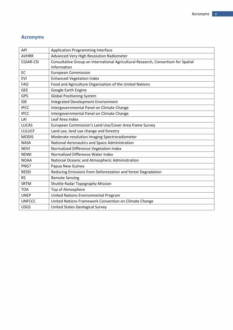
Acronyms
API Application Programming Interface
AVHRR Advanced Very High Resolution Radiometer
CGIAR-CSI Consultative Group on International Agricultural Research, Consortium for Spatial Information
EC European Commission
EVI Enhanced Vegetation Index
FAO Food and Agriculture Organization of the United Nations
GEE Google Earth Engine
GPS Global Positioning System
IDE Integrated Development Environment
IPCC Intergovernmental Panel on Climate Change
IPCC Intergovernmental Panel on Climate Change
LAI Leaf Area Index
LUCAS European Commission’s Land Use/Cover Area frame Survey
LULUCF Land use, land use change and forestry
MODIS Moderate-resolution Imaging Spectroradiometer
NASA National Aeronautics and Space Administration
NDVI Normalized Difference Vegetation Index
NDWI Normalized Difference Water Index
NOAA National Oceanic and Atmospheric Administration
PNG? Papua New Guinea
REDD Reducing Emissions from Deforestation and forest Degradation
RS Remote Sensing
SRTM Shuttle Radar Topography Mission
TOA Top of Atmosphere
UNEP United Nations Environmental Program
UNFCCC United Nations Framework Convention on Climate Change
USGS United States Geological Survey
vi
Contents
Acknowledgements ............................................................................................................................................. iv
Acronyms .............................................................................................................................................................. v
1 Introduction to Collect Earth and its supporting software ......................................................................... 1
1.1 Collect Earth system architecture ....................................................................................................... 1
1.2 Collect Earth system maintenance ...................................................................................................... 3
2 Getting started ............................................................................................................................................ 4
2.1 Installation and setup of Collect Earth ................................................................................................ 4
2.2 Setting up Google Earth ....................................................................................................................... 8
3 Assessing land use and land use change ................................................................................................... 10
3.1 Land use sampling with Collect Earth ................................................................................................ 11
3.1.1 Adding Collect Earth data files .................................................................................................. 12
3.1.2 Entering land use data ............................................................................................................... 15
3.1.3 Modifying the plot layout .......................................................................................................... 17
3.1.4 Exporting Collect Earth data ...................................................................................................... 18
3.1.5 Backing up Collect Earth data .................................................................................................... 18
3.2 Navigating and organizing with Google Earth ................................................................................... 19
3.2.1 Optimizing the data view ........................................................................................................... 19
3.2.2 Finding plots .............................................................................................................................. 19
3.2.3 Improving navigation ................................................................................................................. 20
3.2.4 Measuring distance ................................................................................................................... 21
3.2.5 Viewing historical imagery ........................................................................................................ 22
3.2.6 Exporting images ....................................................................................................................... 23
3.2.7 Adding overlays ......................................................................................................................... 24
3.2.8 Saving KMZ files ......................................................................................................................... 26
3.3 Exploring new perspectives with Bing Maps ..................................................................................... 27
3.4 Visualizing imagery with Google Earth Engine .................................................................................. 27
4 Analyzing data with Saiku Server............................................................................................................... 31
4.1.1 Data visualization....................................................................................................................... 32
4.1.2 Filtering data .............................................................................................................................. 40
4.1.3 Saving and opening queries ....................................................................................................... 44
4.1.4 Export options ........................................................................................................................... 45
4.1.5 Sample queries for land use, land use change and forest (LULUCF) monitoring ...................... 46
vii
5 Processing geospatial data with QGIS ....................................................................................................... 50
5.1 Installation and setup of QGIS ........................................................................................................... 50
5.2 Exporting vector files to Google Earth and Google Earth Engine ...................................................... 51
5.3 Exporting raster files to Google Earth ............................................................................................... 52
5.4 Creating a sampling grid for Collect Earth ......................................................................................... 55
5.4.1 Identify the spatial extent for the grid ...................................................................................... 56
5.4.2 Create a basic grid with round numbers ................................................................................... 58
5.4.3 Reduce the grid layer to only the areas of interest ................................................................... 61
5.4.4 Add coordinates to the grid’s attributes table .......................................................................... 63
5.4.5 Acquire SRTM digital elevation data ......................................................................................... 65
5.4.6 Derive slope and aspect data from digital elevation data ......................................................... 68
5.4.7 Add elevation, slope and aspect data to the grid ...................................................................... 70
5.4.8 Format the grid as a CSV compatible with Collect Earth ........................................................... 74
6 Synergies between the Collect Earth sampling and Wall-to-Wall mapping .............................................. 78
6.1 Preparing vector data in Google Fusion Tables ................................................................................. 78
6.1.1 Importing Collect Earth data into Google Fusion Tables ........................................................... 78
6.1.2 Importing KMLs into Google Fusion Tables ............................................................................... 84
6.2 Getting started with Google Earth Engine ......................................................................................... 85
6.3 Google Earth Engine (GEE) API playground ....................................................................................... 86
6.3.1 Vegetation Indices ..................................................................................................................... 86
6.3.2 Creating a sampling grid for Collect Earth using GEE API code editor ...................................... 89
6.4 Collect Earth data as training sites for a supervised classification .................................................... 94
6.4.1 Add Collect Earth vector data .................................................................................................... 94
6.4.2 Add raster data (Landsat and MODIS) ....................................................................................... 97
6.4.3 Extract and apply the water mask ............................................................................................. 98
6.4.4 Extract the area of interest ...................................................................................................... 100
6.4.5 Train a classifier ....................................................................................................................... 102
6.4.6 Train a classifier and display results ........................................................................................ 103
6.4.7 Review classification results .................................................................................................... 104
6.4.8 Exporting results ...................................................................................................................... 106
6.4.9 Saving and sharing results ....................................................................................................... 107
7 Advanced Collect Earth functionalities.................................................................................................... 107
7.1 Application and data folder ............................................................................................................. 107
7.2 Importing a KML with placemarks ................................................................................................... 108
viii
7.2.1 Creating a .kml file in Google Earth ......................................................................................... 108
7.2.2 Importing a .kml file to Collect Earth ....................................................................................... 111
7.3 Find plots not yet assessed .............................................................................................................. 112
7.3.1 Preparations ............................................................................................................................ 112
7.3.2 Importing the missing plots into Collect Earth ........................................................................ 113
7.4 Printing out the application log ....................................................................................................... 114
7.5 Updating Collect Earth ..................................................................................................................... 114
7.5.1 Updating automatically ........................................................................................................... 114
7.5.2 Updating manually .................................................................................................................. 115
7.6 Updating data on plots already collected ....................................................................................... 116
7.7 Setting up a PostgreSQL database ................................................................................................... 117
7.7.1 Install PostgreSQL .................................................................................................................... 117
7.7.2 Configure the Database ........................................................................................................... 118
7.7.3 Set up Collect Earth ................................................................................................................. 119
Volume II: Collect Earth User Manual for Windows OS
1 Introduction to Collect Earth and its supporting software
1 Introduction to Collect Earth and its supporting software
Collect Earth is a user-friendly, Java-based tool that draws upon a selection of other software to facilitate
data collection. The following training materials include guidance on the use of Collect Earth and most of its
supporting software. This information is also available online and in video format at www.openforis.org.
Documentation on the more technical components of the Collect Earth system (including SQLite and
PostgreSQL) is available on the Collect Earth Github page.1 Collect Earth runs on Windows, Mac and Linux
operating systems.
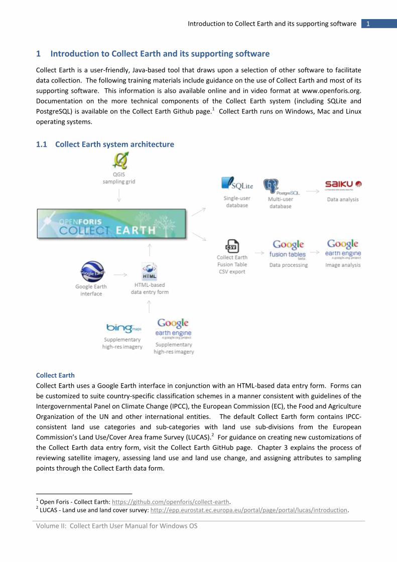
1.1 Collect Earth system architecture
Collect Earth
Collect Earth uses a Google Earth interface in conjunction with an HTML-based data entry form. Forms can
be customized to suite country-specific classification schemes in a manner consistent with guidelines of the
Intergovernmental Panel on Climate Change (IPCC), the European Commission (EC), the Food and Agriculture
Organization of the UN and other international entities. The default Collect Earth form contains IPCC-
consistent land use categories and sub-categories with land use sub-divisions from the European
Commission’s Land Use/Cover Area frame Survey (LUCAS).2 For guidance on creating new customizations of
the Collect Earth data entry form, visit the Collect Earth GitHub page. Chapter 3 explains the process of
reviewing satellite imagery, assessing land use and land use change, and assigning attributes to sampling
points through the Collect Earth data form.
1 Open Foris - Collect Earth: https://github.com/openforis/collect-earth.
2 LUCAS - Land use and land cover survey: http://epp.eurostat.ec.europa.eu/portal/page/portal/lucas/introduction.
Volume II: Collect Earth User Manual for Windows OS
2 Introduction to Collect Earth and its supporting software
Google Earth, Bing Maps and Google Earth Engine (visualization of satellite imagery)
Collect Earth facilitates the interpretation of high and medium spatial resolution imagery in Google Earth,
Bing Maps and Google Earth Engine. Google Earth’s virtual globe is largely comprised of 15 meter resolution
Landsat imagery, 2.5m SPOT imagery and high resolution imagery from several other providers (CNES, Digital
Global, EarthSat, First Base Solutions, GeoEye-1, GlobeXplorer, IKONOS, Pictometry International, Spot
Image, Aerometrex and Sinclair Knight Merz). Microsoft’s Bing Maps presents imagery provided by Digital
Globe ranging from 3m to 30cm resolution. Google Earth Engine’s web-based platform facilitates access to
United States Geological Survey 30m resolution Landsat imagery. Collect Earth synchronizes the view of
each sampling point across all three platforms.
The imagery used within Google Earth, Bing Maps and Google Earth Engine differ not only in their spatial
resolution, but also in their temporal resolution. Collect Earth enables users to enter data regarding current
land use and historical land use changes. Users can determine the reference period most appropriate for
their land use monitoring objectives. The IPCC recommends a reference period of at least 20 years based on
the amount of time needed for dead organic matter and soil carbon stocks to reach equilibrium following
land-use conversion.3 Most of the imagery available in Bing Maps and Google Earth have been acquired at
very irregular intervals over the past 10 years. In contrast, Earth Engine contains over 40 years of imagery
that has been acquired every 16 days. The description of how to use Collect Earth in Chapter 3 includes
guidance on navigating the strengths and weakness of these three imagery repositories to develop a more
complete understanding of land use, land use change and forestry in a given site.
SQLite and PostgreSQL
The data entered in Collect Earth is automatically saved to a database. Collect Earth can be configured for a
single-user environment with a SQLite database. This arrangement is best for either individual users or for
geographically disperse team. A PostgreSQL database is recommended for multi-user environments,
particularly where users will work from a shared network. The PostgreSQL configuration of Collect Earth
facilitates collaborate work by allowing users to see in real time when new data has been entered. It also
makes it easier for an administrator to review the work of others for quality control purposes.
Saiku Server
Both types of databases automatically populate Saiku Server, an open-source web-based software produced
by Meteorite consulting. A version of this open-source software has been customized for visualizing and
analyzing Collect Earth data. Countries using Collect Earth for a national land use assessment may generate
data in Collect Earth for tens of thousands of points. Saiku organizes this wealth of information and enables
users to run queries on the data and immediately view the results in tabular format or as graphs. Chapter 4
explains how Saiku users to can quickly identify trends and prepare inputs for LULUCF reporting to the
UNFCCC and other entities involved in the sector.
Google Earth Engine (image processing and analysis)
Collect Earth facilitates land use assessment through a sampling approach rather than wall-to-wall mapping.
However, land use data (point vector files) generated with Collect Earth can be used as training sites for wall-
3 IPCC (2006) Guidelines for National Greenhouse Gas Inventories. Volume 4: Agriculture, Forestry and Other Land Use,
Chapter 3: Consistent Representation of Lands.
Volume II: Collect Earth User Manual for Windows OS
3 Introduction to Collect Earth and its supporting software
to-wall image classifications. Chapter 6 reviews the procedure for using Collect Earth data to conduct a
supervised (wall-to-wall) classification in Google Earth Engine.
QGIS
QGIS is a free and open-source geographic information system that can be used to process data that can
support the land use classification process. Where existing land use or land cover data is available in a
spatial format, users can convert vector (points, line, polygons) and raster (images) data into KML files that
can be viewed in Google Earth during a land use classification with Collect Earth. KML files are also
compatible with Google Fusion Tables and can be imported into Google Earth Engine.
Chapter 5 provides instructions on converting spatial data and also creating a sampling grid. A default,
coarse (5km x 5km) grid of sampling points is available for download on the Collect Earth website. However,
a medium or a fine scale grid comprised of more points is recommended for a full and robust LULUCF
assessment for a country or sub-national project site. Chapter 5 explains the process of generating a
sampling grid and populating its attributes table to ensure compatibility with Collect Earth.
1.2 Collect Earth system maintenance Collect Earth is continuously being improved. The software and its various components (Java, Google Earth,
etc) will need to be updated as new releases become available. The Collect Earth development team will
notify users of future releases and recommended upgrades through the Collect Earth website, its GitHub
page and through the Collect Earth users’ network. Visit the Collect Earth website to subscribe to the
network’s listserv.4
4 Collect Earth user network registration page: ADD LINK
Volume II: Collect Earth User Manual for Windows OS
4 Getting started
2 Getting started
2.1 Installation and setup of Collect Earth
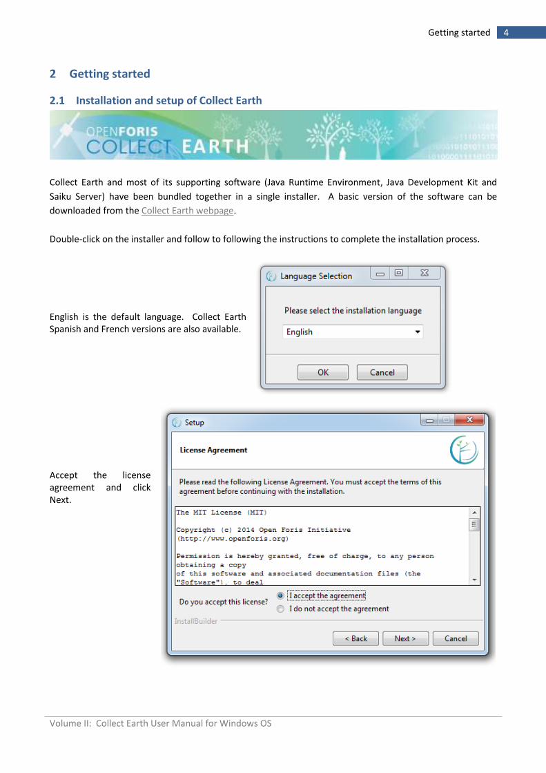
Collect Earth and most of its supporting software (Java Runtime Environment, Java Development Kit and
Saiku Server) have been bundled together in a single installer. A basic version of the software can be
downloaded from the Collect Earth webpage.
Double-click on the installer and follow to following the instructions to complete the installation process.
English is the default language. Collect Earth Spanish and French versions are also available.
Accept the license agreement and click Next.
Volume II: Collect Earth User Manual for Windows OS
5 Getting started
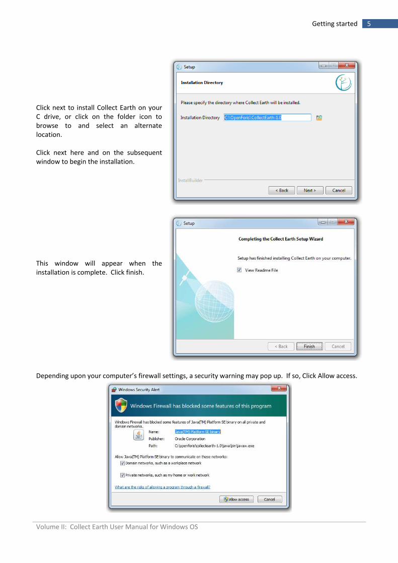
Click next to install Collect Earth on your C drive, or click on the folder icon to browse to and select an alternate location. Click next here and on the subsequent window to begin the installation.
This window will appear when the installation is complete. Click finish.
Depending upon your computer’s firewall settings, a security warning may pop up. If so, Click Allow access.
Volume II: Collect Earth User Manual for Windows OS
6 Getting started
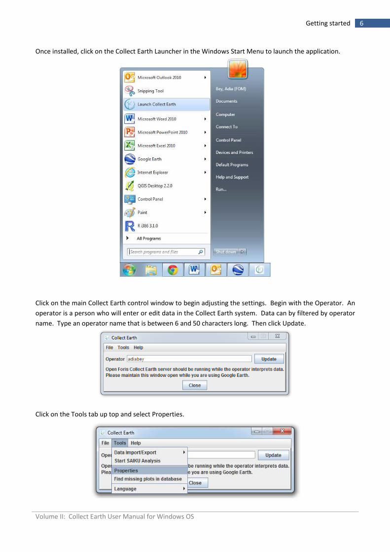
Once installed, click on the Collect Earth Launcher in the Windows Start Menu to launch the application.
Click on the main Collect Earth control window to begin adjusting the settings. Begin with the Operator. An
operator is a person who will enter or edit data in the Collect Earth system. Data can by filtered by operator
name. Type an operator name that is between 6 and 50 characters long. Then click Update.
Click on the Tools tab up top and select Properties.
Volume II: Collect Earth User Manual for Windows OS
7 Getting started
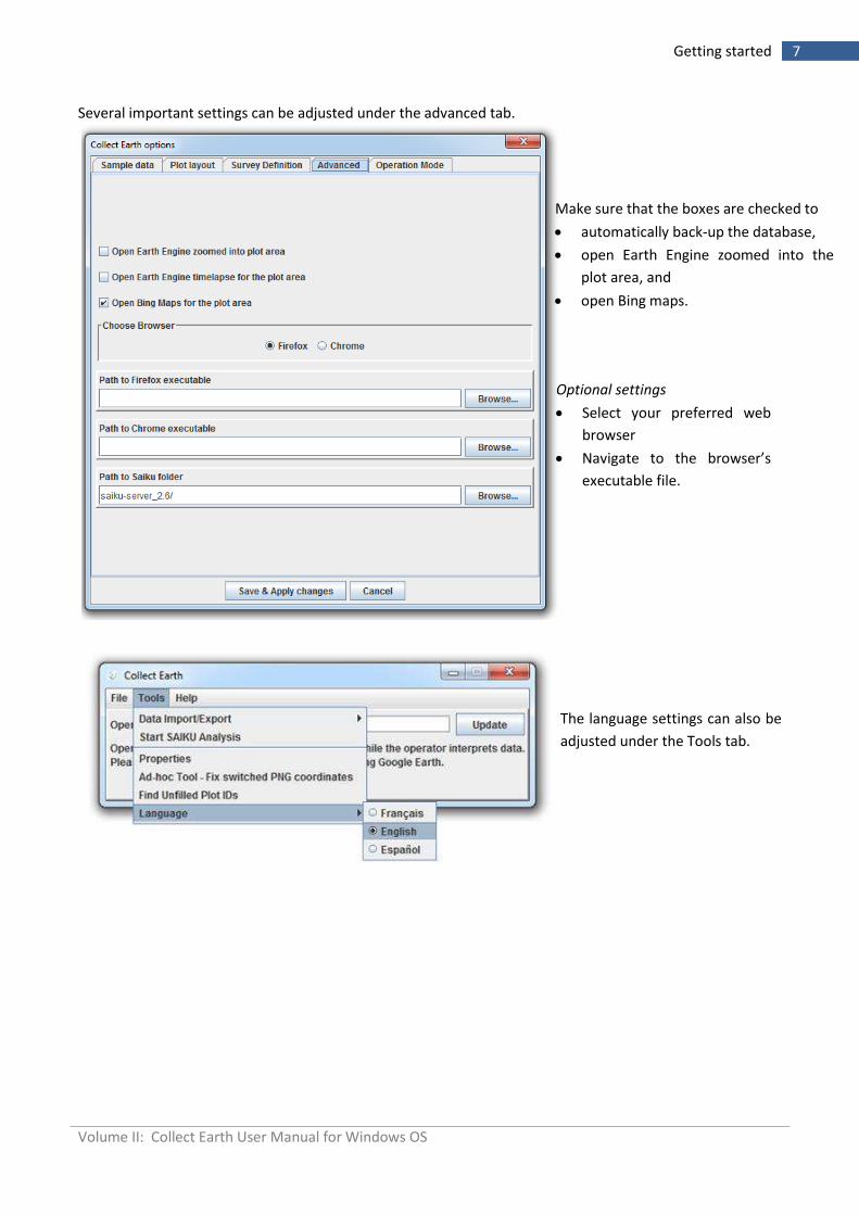
Several important settings can be adjusted under the advanced tab.
Optional settings
Select your preferred web
browser
Navigate to the browser’s
executable file.
The language settings can also be
adjusted under the Tools tab.
Make sure that the boxes are checked to
automatically back-up the database,
open Earth Engine zoomed into the
plot area, and
open Bing maps.
Volume II: Collect Earth User Manual for Windows OS
8 Getting started
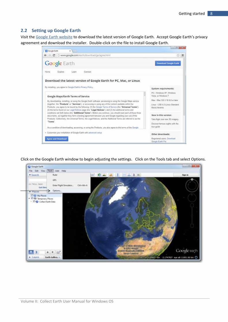
2.2 Setting up Google Earth
Visit the Google Earth website to download the latest version of Google Earth. Accept Google Earth’s privacy
agreement and download the installer. Double-click on the file to install Google Earth.
Click on the Google Earth window to begin adjusting the settings. Click on the Tools tab and select Options.
Volume II: Collect Earth User Manual for Windows OS
9 Getting started
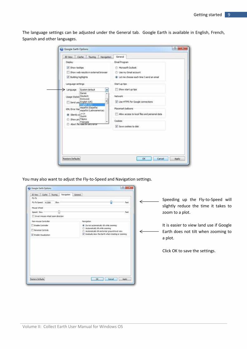
The language settings can be adjusted under the General tab. Google Earth is available in English, French,
Spanish and other languages.
You may also want to adjust the Fly-to-Speed and Navigation settings.
Speeding up the Fly-to-Speed will
slightly reduce the time it takes to
zoom to a plot.
It is easier to view land use if Google
Earth does not tilt when zooming to
a plot.
Click OK to save the settings.
Volume II: Collect Earth User Manual for Windows OS
10 Assessing land use and land use change
3 Assessing land use and land use change
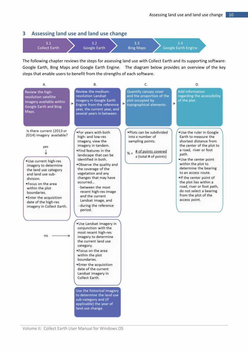
The following chapter reviews the steps for assessing land use with Collect Earth and its supporting software:
Google Earth, Bing Maps and Google Earth Engine. The diagram below provides an overview of the key
steps that enable users to benefit from the strengths of each software.
3.1 Collect Earth
3.2 Google Earth
3.3 Bing Maps
3.4 Google Earth Engine
Volume II: Collect Earth User Manual for Windows OS
11 Assessing land use and land use change
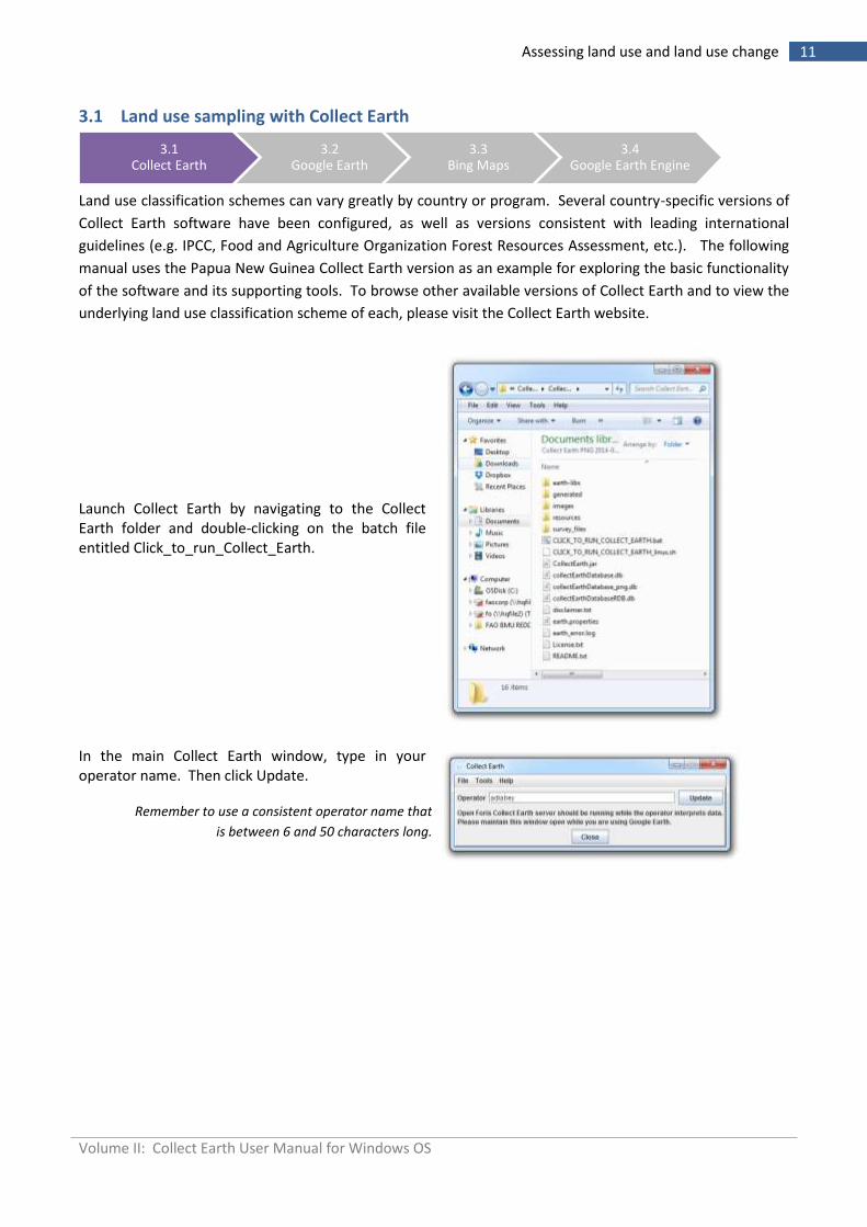
3.1 Land use sampling with Collect Earth
Land use classification schemes can vary greatly by country or program. Several country-specific versions of
Collect Earth software have been configured, as well as versions consistent with leading international
guidelines (e.g. IPCC, Food and Agriculture Organization Forest Resources Assessment, etc.). The following
manual uses the Papua New Guinea Collect Earth version as an example for exploring the basic functionality
of the software and its supporting tools. To browse other available versions of Collect Earth and to view the
underlying land use classification scheme of each, please visit the Collect Earth website.
Launch Collect Earth by navigating to the Collect Earth folder and double-clicking on the batch file entitled Click_to_run_Collect_Earth.
In the main Collect Earth window, type in your operator name. Then click Update.
3.1 Collect Earth
3.2 Google Earth
3.3 Bing Maps
3.4 Google Earth Engine
Remember to use a consistent operator name that
is between 6 and 50 characters long.
Volume II: Collect Earth User Manual for Windows OS
12 Assessing land use and land use change
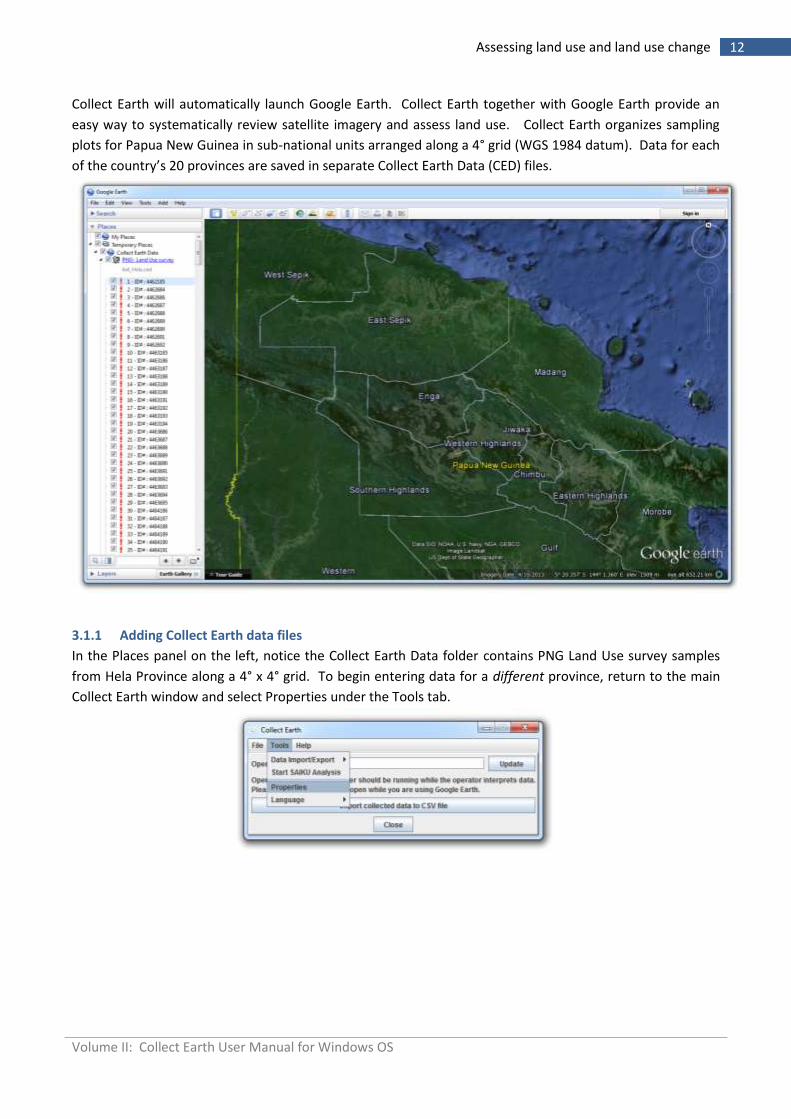
Collect Earth will automatically launch Google Earth. Collect Earth together with Google Earth provide an
easy way to systematically review satellite imagery and assess land use. Collect Earth organizes sampling
plots for Papua New Guinea in sub-national units arranged along a 4° grid (WGS 1984 datum). Data for each
of the country’s 20 provinces are saved in separate Collect Earth Data (CED) files.
3.1.1 Adding Collect Earth data files
In the Places panel on the left, notice the Collect Earth Data folder contains PNG Land Use survey samples
from Hela Province along a 4° x 4° grid. To begin entering data for a different province, return to the main
Collect Earth window and select Properties under the Tools tab.
Volume II: Collect Earth User Manual for Windows OS
13 Assessing land use and land use change
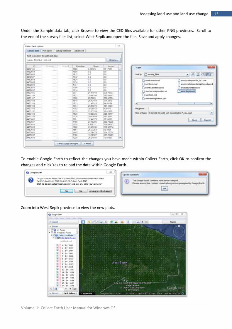
Under the Sample data tab, click Browse to view the CED files available for other PNG provinces. Scroll to
the end of the survey files list, select West Sepik and open the file. Save and apply changes.
To enable Google Earth to reflect the changes you have made within Collect Earth, click OK to confirm the
changes and click Yes to reload the data within Google Earth.
Zoom into West Sepik province to view the new plots.
Volume II: Collect Earth User Manual for Windows OS
14 Assessing land use and land use change
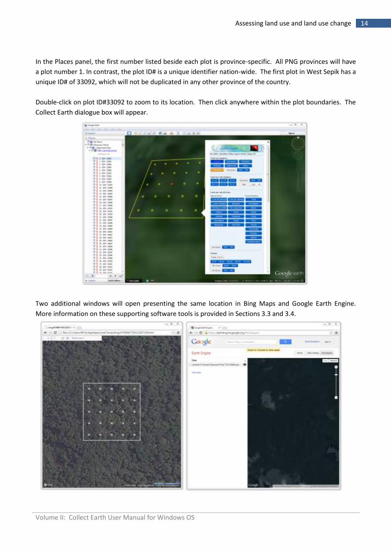
In the Places panel, the first number listed beside each plot is province-specific. All PNG provinces will have
a plot number 1. In contrast, the plot ID# is a unique identifier nation-wide. The first plot in West Sepik has a
unique ID# of 33092, which will not be duplicated in any other province of the country.
Double-click on plot ID#33092 to zoom to its location. Then click anywhere within the plot boundaries. The
Collect Earth dialogue box will appear.
Two additional windows will open presenting the same location in Bing Maps and Google Earth Engine.
More information on these supporting software tools is provided in Sections 3.3 and 3.4.
Volume II: Collect Earth User Manual for Windows OS
15 Assessing land use and land use change
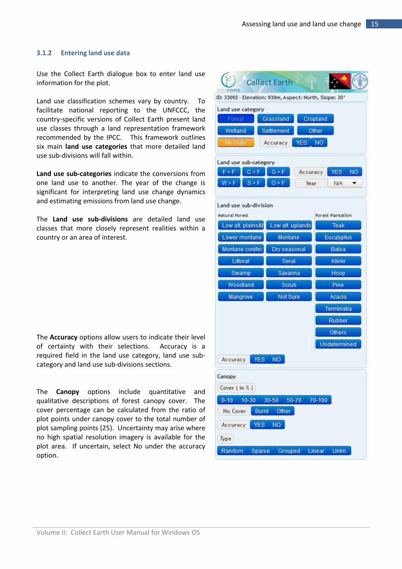
3.1.2 Entering land use data
Use the Collect Earth dialogue box to enter land use information for the plot. Land use classification schemes vary by country. To facilitate national reporting to the UNFCCC, the country-specific versions of Collect Earth present land use classes through a land representation framework recommended by the IPCC. This framework outlines six main land use categories that more detailed land use sub-divisions will fall within. Land use sub-categories indicate the conversions from one land use to another. The year of the change is significant for interpreting land use change dynamics and estimating emissions from land use change. The Land use sub-divisions are detailed land use classes that more closely represent realities within a country or an area of interest. The Accuracy options allow users to indicate their level of certainty with their selections. Accuracy is a required field in the land use category, land use sub-category and land use sub-divisions sections. The Canopy options include quantitative and qualitative descriptions of forest canopy cover. The cover percentage can be calculated from the ratio of plot points under canopy cover to the total number of plot sampling points (25). Uncertainty may arise where no high spatial resolution imagery is available for the plot area. If uncertain, select No under the accuracy option.
Volume II: Collect Earth User Manual for Windows OS
16 Assessing land use and land use change
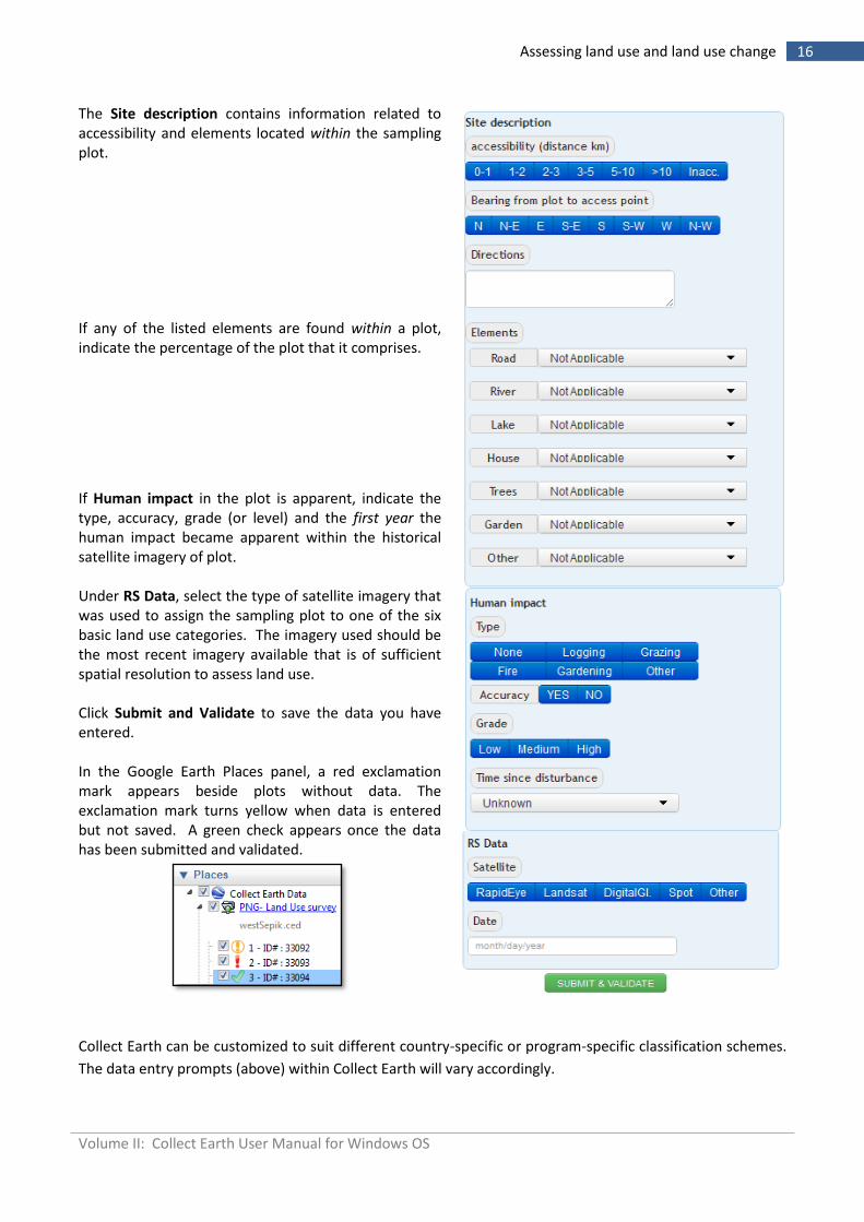
The Site description contains information related to accessibility and elements located within the sampling plot. If any of the listed elements are found within a plot, indicate the percentage of the plot that it comprises.
If Human impact in the plot is apparent, indicate the type, accuracy, grade (or level) and the first year the human impact became apparent within the historical satellite imagery of plot. Under RS Data, select the type of satellite imagery that was used to assign the sampling plot to one of the six basic land use categories. The imagery used should be the most recent imagery available that is of sufficient spatial resolution to assess land use. Click Submit and Validate to save the data you have entered. In the Google Earth Places panel, a red exclamation mark appears beside plots without data. The exclamation mark turns yellow when data is entered but not saved. A green check appears once the data has been submitted and validated.
Collect Earth can be customized to suit different country-specific or program-specific classification schemes.
The data entry prompts (above) within Collect Earth will vary accordingly.
Volume II: Collect Earth User Manual for Windows OS
17 Assessing land use and land use change
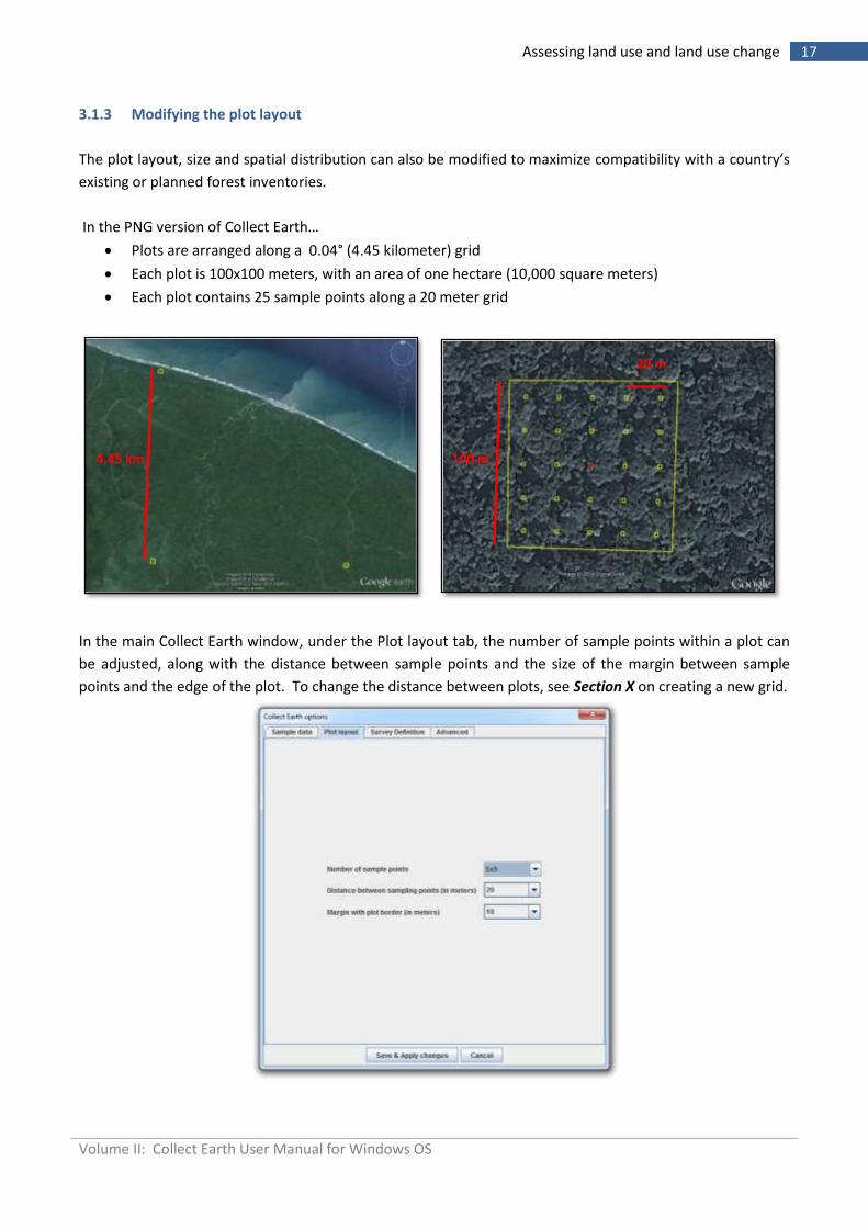
3.1.3 Modifying the plot layout
The plot layout, size and spatial distribution can also be modified to maximize compatibility with a country’s
existing or planned forest inventories.
In the PNG version of Collect Earth…
Plots are arranged along a 0.04° (4.45 kilometer) grid
Each plot is 100x100 meters, with an area of one hectare (10,000 square meters)
Each plot contains 25 sample points along a 20 meter grid
In the main Collect Earth window, under the Plot layout tab, the number of sample points within a plot can
be adjusted, along with the distance between sample points and the size of the margin between sample
points and the edge of the plot. To change the distance between plots, see Section X on creating a new grid.
4.45 km
kmm
100 m
kmm
20 m
kmm
Volume II: Collect Earth User Manual for Windows OS
18 Assessing land use and land use change
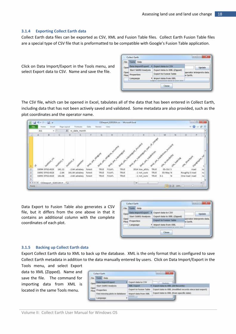
3.1.4 Exporting Collect Earth data
Collect Earth data files can be exported as CSV, XML and Fusion Table files. Collect Earth Fusion Table files
are a special type of CSV file that is preformatted to be compatible with Google’s Fusion Table application.
Click on Data Import/Export in the Tools menu, and select Export data to CSV. Name and save the file.
The CSV file, which can be opened in Excel, tabulates all of the data that has been entered in Collect Earth,
including data that has not been actively saved and validated. Some metadata are also provided, such as the
plot coordinates and the operator name.
Data Export to Fusion Table also generates a CSV file, but it differs from the one above in that it contains an additional column with the complete coordinates of each plot.
3.1.5 Backing up Collect Earth data
Export Collect Earth data to XML to back up the database. XML is the only format that is configured to save
Collect Earth metadata in addition to the data manually entered by users. Click on Data Import/Export in the
Tools menu, and select Export
data to XML (Zipped). Name and
save the file. The command for
importing data from XML is
located in the same Tools menu.
Volume II: Collect Earth User Manual for Windows OS
19 Assessing land use and land use change
3.2 Navigating and organizing with Google Earth
Google Earth serves as the main interface for Collect Earth software. Adjusting certain settings and
familiarizing yourself with the basic functionality of Google Earth can enhance the experience of using
Collect Earth. Below are a few tips.
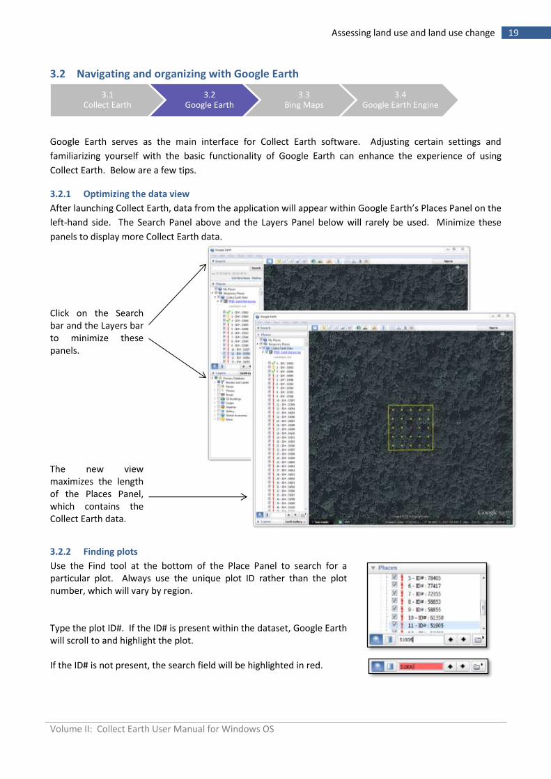
3.2.1 Optimizing the data view
After launching Collect Earth, data from the application will appear within Google Earth’s Places Panel on the
left-hand side. The Search Panel above and the Layers Panel below will rarely be used. Minimize these
panels to display more Collect Earth data.
Click on the Search bar and the Layers bar to minimize these panels.
The new view maximizes the length of the Places Panel, which contains the Collect Earth data.
3.2.2 Finding plots
Use the Find tool at the bottom of the Place Panel to search for a particular plot. Always use the unique plot ID rather than the plot number, which will vary by region. Type the plot ID#. If the ID# is present within the dataset, Google Earth will scroll to and highlight the plot. If the ID# is not present, the search field will be highlighted in red.
3.1 Collect Earth
3.2 Google Earth
3.3 Bing Maps
3.4 Google Earth Engine
Volume II: Collect Earth User Manual for Windows OS
20 Assessing land use and land use change
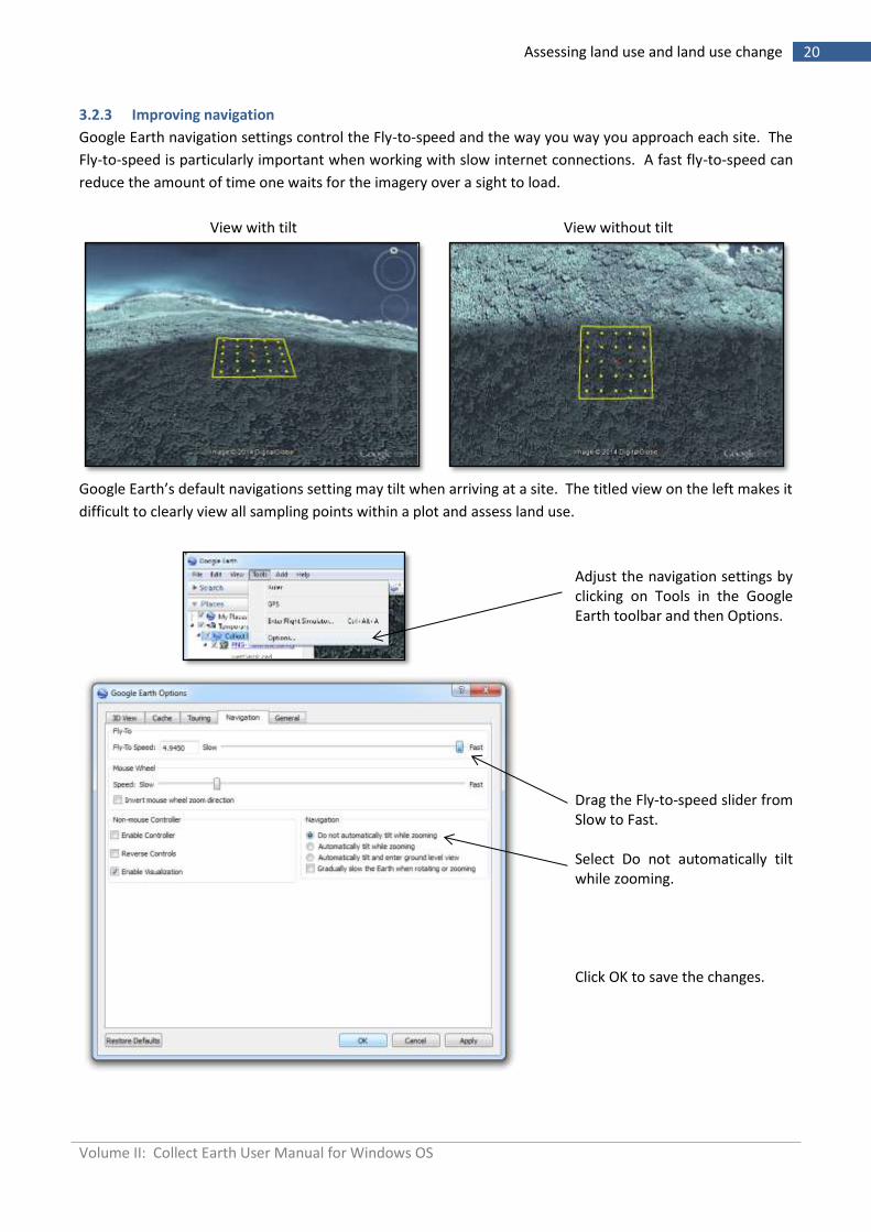
3.2.3 Improving navigation
Google Earth navigation settings control the Fly-to-speed and the way you way you approach each site. The
Fly-to-speed is particularly important when working with slow internet connections. A fast fly-to-speed can
reduce the amount of time one waits for the imagery over a sight to load.
View with tilt View without tilt
Google Earth’s default navigations setting may tilt when arriving at a site. The titled view on the left makes it
difficult to clearly view all sampling points within a plot and assess land use.
Adjust the navigation settings by clicking on Tools in the Google Earth toolbar and then Options.
Drag the Fly-to-speed slider from Slow to Fast. Select Do not automatically tilt while zooming. Click OK to save the changes.
Volume II: Collect Earth User Manual for Windows OS
21 Assessing land use and land use change
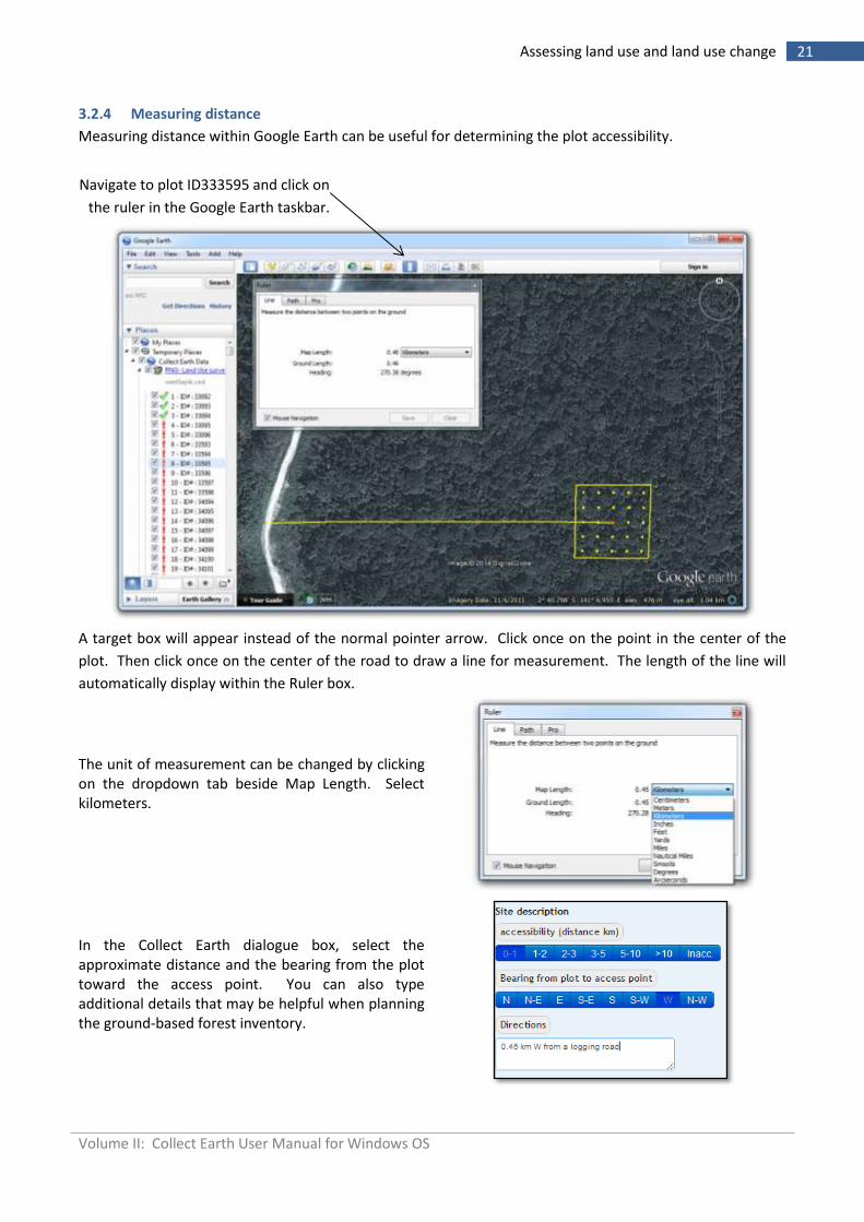
3.2.4 Measuring distance
Measuring distance within Google Earth can be useful for determining the plot accessibility.
A target box will appear instead of the normal pointer arrow. Click once on the point in the center of the
plot. Then click once on the center of the road to draw a line for measurement. The length of the line will
automatically display within the Ruler box.
The unit of measurement can be changed by clicking on the dropdown tab beside Map Length. Select kilometers.
In the Collect Earth dialogue box, select the approximate distance and the bearing from the plot toward the access point. You can also type additional details that may be helpful when planning the ground-based forest inventory.
Navigate to plot ID333595 and click on
the ruler in the Google Earth taskbar.
Volume II: Collect Earth User Manual for Windows OS
22 Assessing land use and land use change
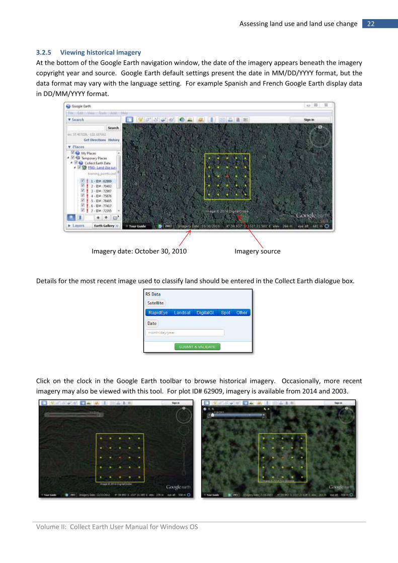
3.2.5 Viewing historical imagery
At the bottom of the Google Earth navigation window, the date of the imagery appears beneath the imagery
copyright year and source. Google Earth default settings present the date in MM/DD/YYYY format, but the
data format may vary with the language setting. For example Spanish and French Google Earth display data
in DD/MM/YYYY format.
Imagery date: October 30, 2010 Imagery source
Details for the most recent image used to classify land should be entered in the Collect Earth dialogue box.
Click on the clock in the Google Earth toolbar to browse historical imagery. Occasionally, more recent
imagery may also be viewed with this tool. For plot ID# 62909, imagery is available from 2014 and 2003.
Volume II: Collect Earth User Manual for Windows OS
23 Assessing land use and land use change
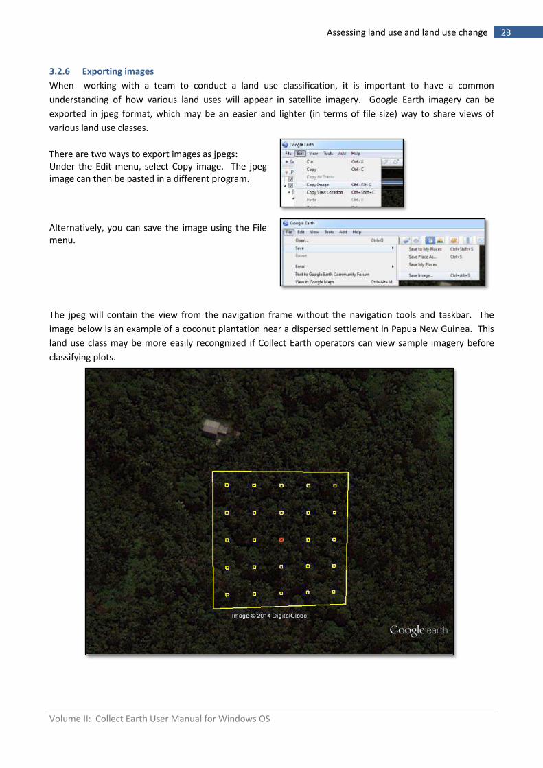
3.2.6 Exporting images
When working with a team to conduct a land use classification, it is important to have a common
understanding of how various land uses will appear in satellite imagery. Google Earth imagery can be
exported in jpeg format, which may be an easier and lighter (in terms of file size) way to share views of
various land use classes.
There are two ways to export images as jpegs: Under the Edit menu, select Copy image. The jpeg image can then be pasted in a different program. Alternatively, you can save the image using the File menu.
The jpeg will contain the view from the navigation frame without the navigation tools and taskbar. The
image below is an example of a coconut plantation near a dispersed settlement in Papua New Guinea. This
land use class may be more easily recongnized if Collect Earth operators can view sample imagery before
classifying plots.
Volume II: Collect Earth User Manual for Windows OS
24 Assessing land use and land use change
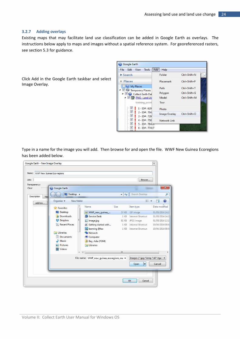
3.2.7 Adding overlays
Existing maps that may facilitate land use classification can be added in Google Earth as overlays. The
instructions below apply to maps and images without a spatial reference system. For georeferenced rasters,
see section 5.3 for guidance.
Click Add in the Google Earth taskbar and select Image Overlay.
Type in a name for the image you will add. Then browse for and open the file. WWF New Guinea Ecoregions
has been added below.
Volume II: Collect Earth User Manual for Windows OS
25 Assessing land use and land use change
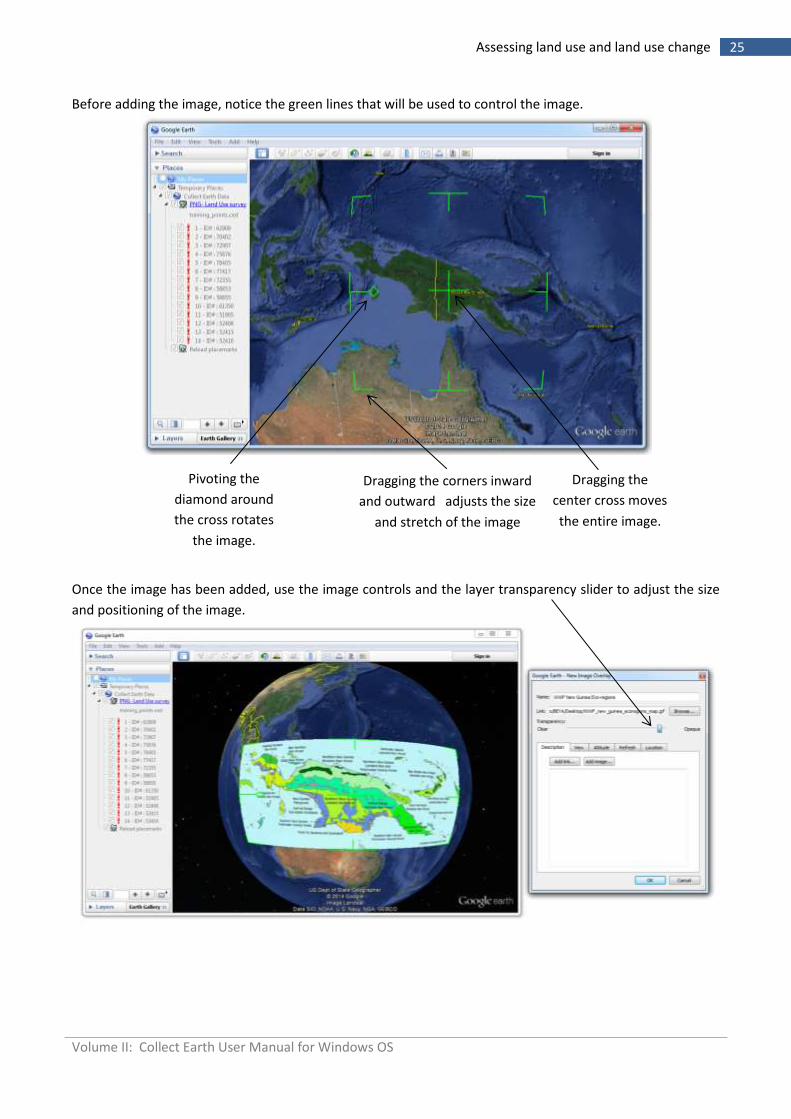
Before adding the image, notice the green lines that will be used to control the image.
Once the image has been added, use the image controls and the layer transparency slider to adjust the size
and positioning of the image.
Dragging the corners inward
and outward adjusts the size
and stretch of the image
Dragging the
center cross moves
the entire image.
Pivoting the
diamond around
the cross rotates
the image.
Volume II: Collect Earth User Manual for Windows OS
26 Assessing land use and land use change
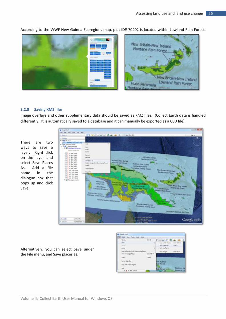
According to the WWF New Guinea Ecoregions map, plot ID# 70402 is located within Lowland Rain Forest.
3.2.8 Saving KMZ files
Image overlays and other supplementary data should be saved as KMZ files. (Collect Earth data is handled
differently. It is automatically saved to a database and it can manually be exported as a CED file).
There are two ways to save a layer. Right click on the layer and select Save Places As. Add a file name in the dialogue box that pops up and click Save.
Alternatively, you can select Save under the File menu, and Save places as.
Volume II: Collect Earth User Manual for Windows OS
27 Assessing land use and land use change
3.3 Exploring new perspectives with Bing Maps
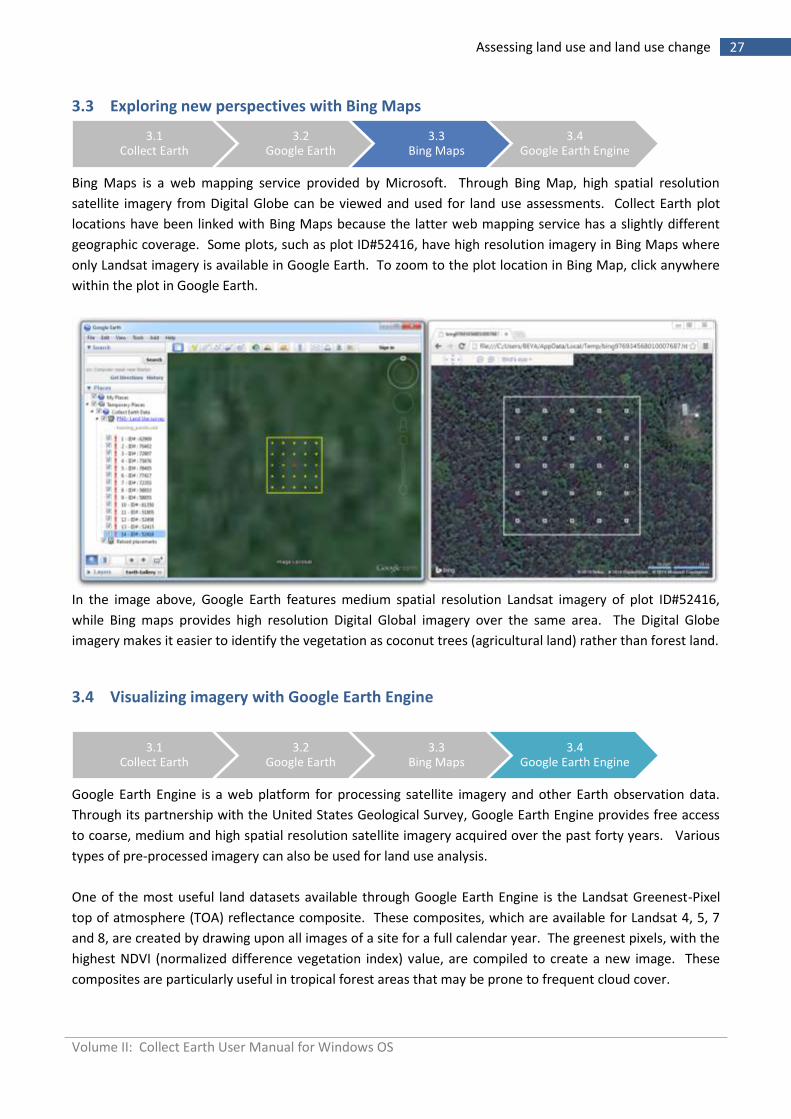
Bing Maps is a web mapping service provided by Microsoft. Through Bing Map, high spatial resolution
satellite imagery from Digital Globe can be viewed and used for land use assessments. Collect Earth plot
locations have been linked with Bing Maps because the latter web mapping service has a slightly different
geographic coverage. Some plots, such as plot ID#52416, have high resolution imagery in Bing Maps where
only Landsat imagery is available in Google Earth. To zoom to the plot location in Bing Map, click anywhere
within the plot in Google Earth.
In the image above, Google Earth features medium spatial resolution Landsat imagery of plot ID#52416,
while Bing maps provides high resolution Digital Global imagery over the same area. The Digital Globe
imagery makes it easier to identify the vegetation as coconut trees (agricultural land) rather than forest land.
3.4 Visualizing imagery with Google Earth Engine
Google Earth Engine is a web platform for processing satellite imagery and other Earth observation data.
Through its partnership with the United States Geological Survey, Google Earth Engine provides free access
to coarse, medium and high spatial resolution satellite imagery acquired over the past forty years. Various
types of pre-processed imagery can also be used for land use analysis.
One of the most useful land datasets available through Google Earth Engine is the Landsat Greenest-Pixel
top of atmosphere (TOA) reflectance composite. These composites, which are available for Landsat 4, 5, 7
and 8, are created by drawing upon all images of a site for a full calendar year. The greenest pixels, with the
highest NDVI (normalized difference vegetation index) value, are compiled to create a new image. These
composites are particularly useful in tropical forest areas that may be prone to frequent cloud cover.
3.1 Collect Earth
3.2 Google Earth
3.3 Bing Maps
3.4 Google Earth Engine
3.1 Collect Earth
3.2 Google Earth
3.3 Bing Maps
3.4 Google Earth Engine
Volume II: Collect Earth User Manual for Windows OS
28 Assessing land use and land use change
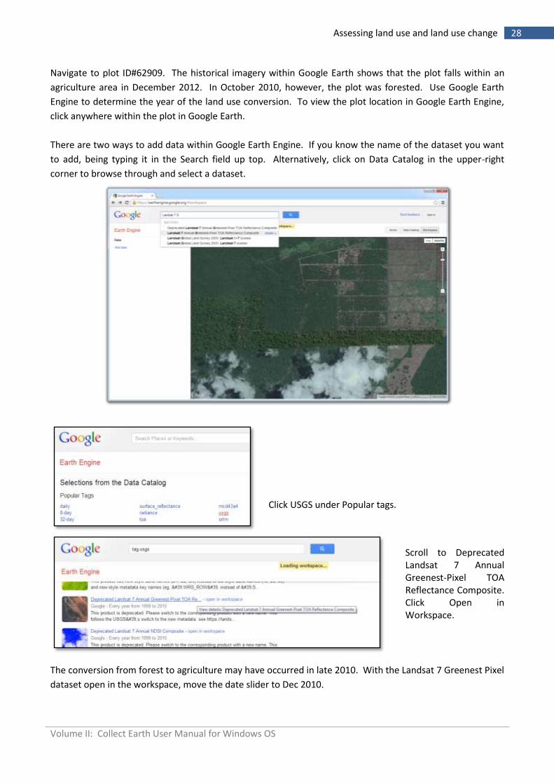
Navigate to plot ID#62909. The historical imagery within Google Earth shows that the plot falls within an
agriculture area in December 2012. In October 2010, however, the plot was forested. Use Google Earth
Engine to determine the year of the land use conversion. To view the plot location in Google Earth Engine,
click anywhere within the plot in Google Earth.
There are two ways to add data within Google Earth Engine. If you know the name of the dataset you want
to add, being typing it in the Search field up top. Alternatively, click on Data Catalog in the upper-right
corner to browse through and select a dataset.
Click USGS under Popular tags.
Scroll to Deprecated Landsat 7 Annual Greenest-Pixel TOA Reflectance Composite. Click Open in Workspace.
The conversion from forest to agriculture may have occurred in late 2010. With the Landsat 7 Greenest Pixel
dataset open in the workspace, move the date slider to Dec 2010.
Volume II: Collect Earth User Manual for Windows OS
29 Assessing land use and land use change
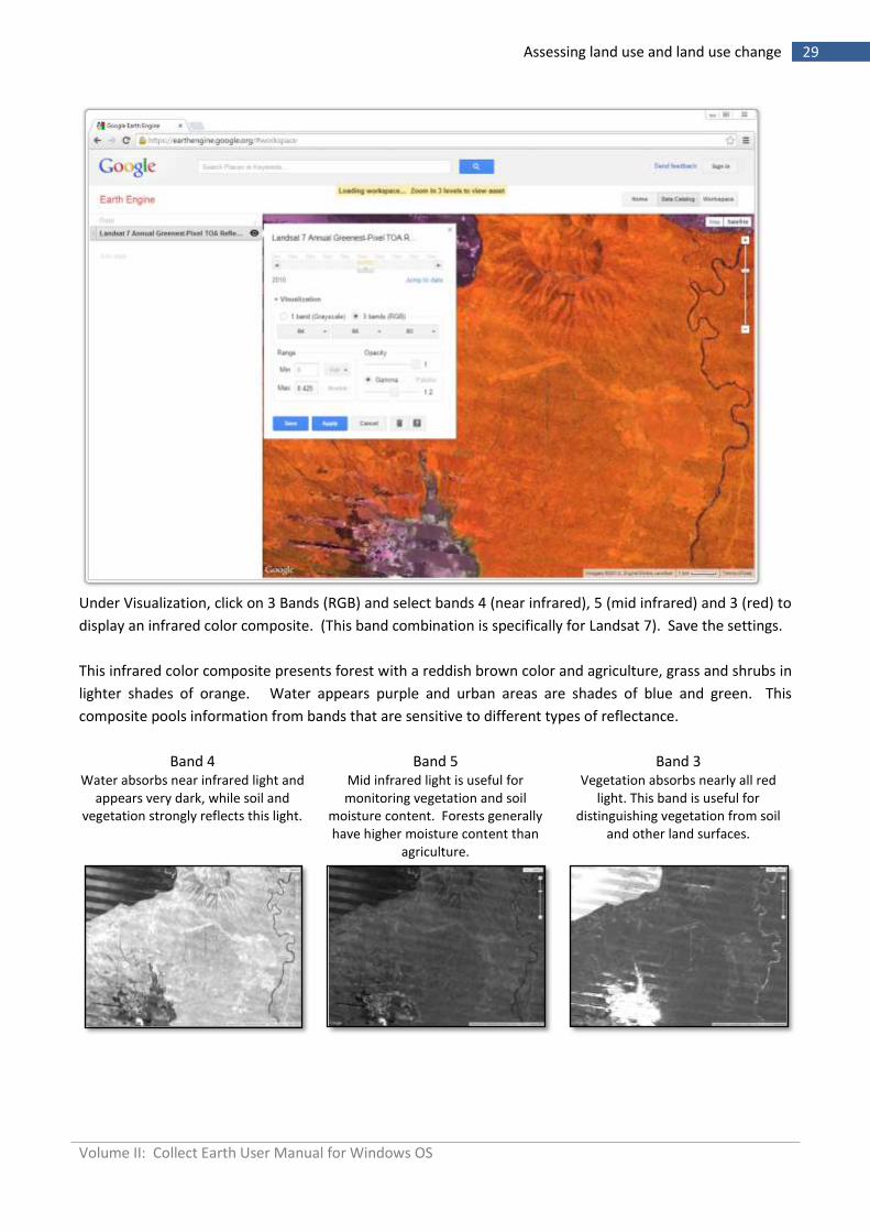
Under Visualization, click on 3 Bands (RGB) and select bands 4 (near infrared), 5 (mid infrared) and 3 (red) to
display an infrared color composite. (This band combination is specifically for Landsat 7). Save the settings.
This infrared color composite presents forest with a reddish brown color and agriculture, grass and shrubs in
lighter shades of orange. Water appears purple and urban areas are shades of blue and green. This
composite pools information from bands that are sensitive to different types of reflectance.
Band 4 Band 5 Band 3 Water absorbs near infrared light and
appears very dark, while soil and vegetation strongly reflects this light.
Mid infrared light is useful for monitoring vegetation and soil
moisture content. Forests generally have higher moisture content than
agriculture.
Vegetation absorbs nearly all red light. This band is useful for
distinguishing vegetation from soil and other land surfaces.
Volume II: Collect Earth User Manual for Windows OS
30 Assessing land use and land use change
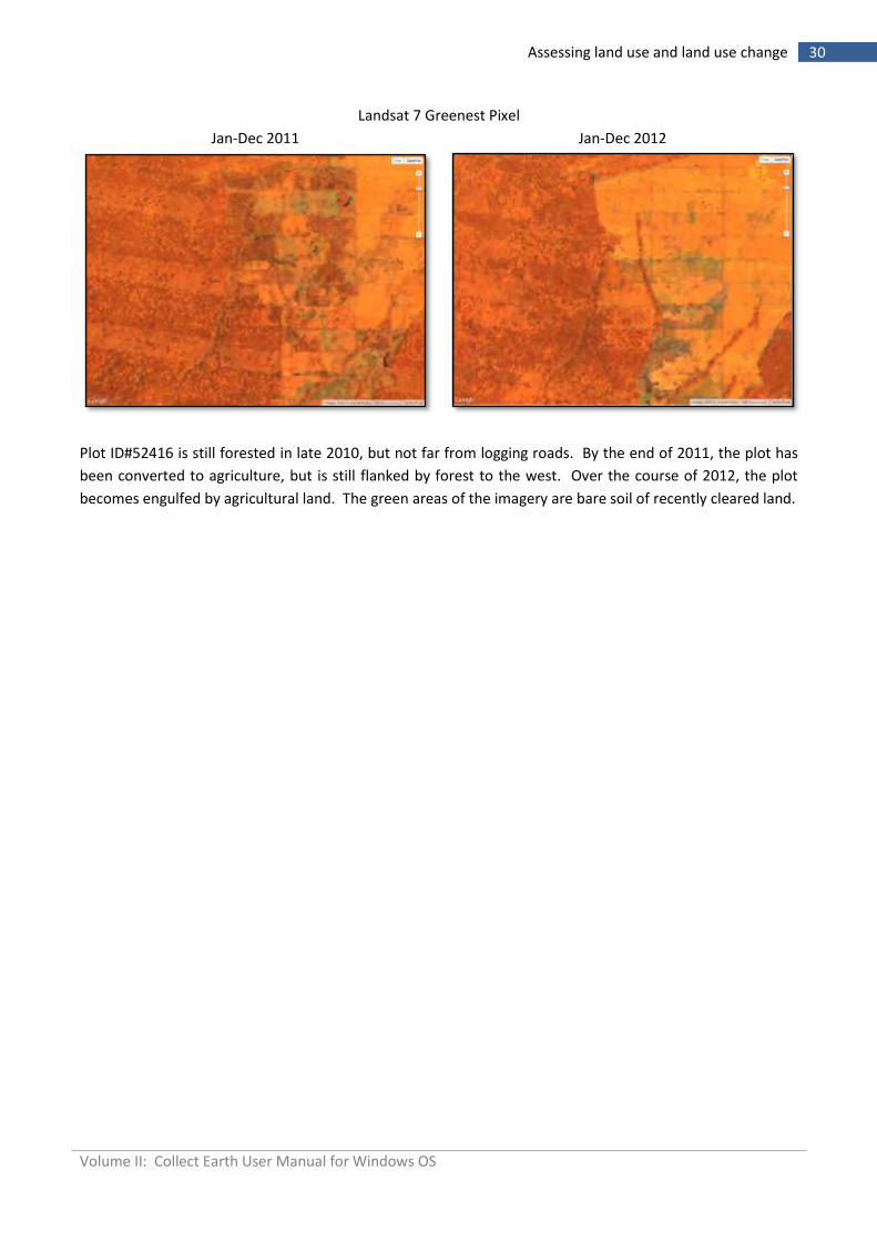
Landsat 7 Greenest Pixel
Jan-Dec 2011 Jan-Dec 2012
Plot ID#52416 is still forested in late 2010, but not far from logging roads. By the end of 2011, the plot has
been converted to agriculture, but is still flanked by forest to the west. Over the course of 2012, the plot
becomes engulfed by agricultural land. The green areas of the imagery are bare soil of recently cleared land.
Volume II: Collect Earth User Manual for Windows OS
31 Analyzing data with Saiku Server
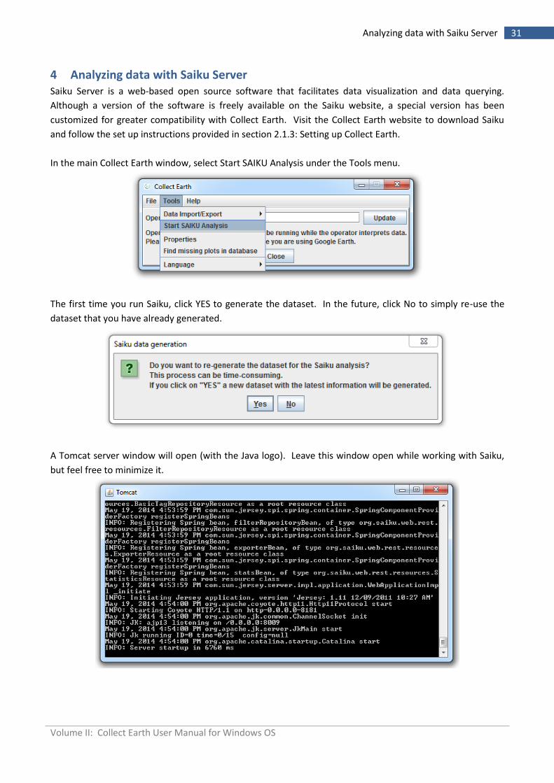
4 Analyzing data with Saiku Server Saiku Server is a web-based open source software that facilitates data visualization and data querying.
Although a version of the software is freely available on the Saiku website, a special version has been
customized for greater compatibility with Collect Earth. Visit the Collect Earth website to download Saiku
and follow the set up instructions provided in section 2.1.3: Setting up Collect Earth.
In the main Collect Earth window, select Start SAIKU Analysis under the Tools menu.
The first time you run Saiku, click YES to generate the dataset. In the future, click No to simply re-use the
dataset that you have already generated.
A Tomcat server window will open (with the Java logo). Leave this window open while working with Saiku,
but feel free to minimize it.
Volume II: Collect Earth User Manual for Windows OS
32 Analyzing data with Saiku Server
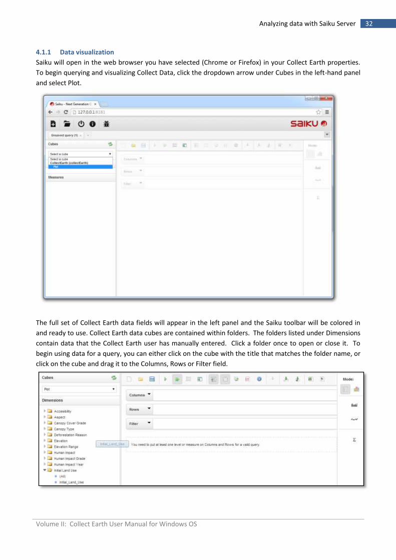
4.1.1 Data visualization
Saiku will open in the web browser you have selected (Chrome or Firefox) in your Collect Earth properties.
To begin querying and visualizing Collect Data, click the dropdown arrow under Cubes in the left-hand panel
and select Plot.
The full set of Collect Earth data fields will appear in the left panel and the Saiku toolbar will be colored in
and ready to use. Collect Earth data cubes are contained within folders. The folders listed under Dimensions
contain data that the Collect Earth user has manually entered. Click a folder once to open or close it. To
begin using data for a query, you can either click on the cube with the title that matches the folder name, or
click on the cube and drag it to the Columns, Rows or Filter field.
Volume II: Collect Earth User Manual for Windows OS
33 Analyzing data with Saiku Server
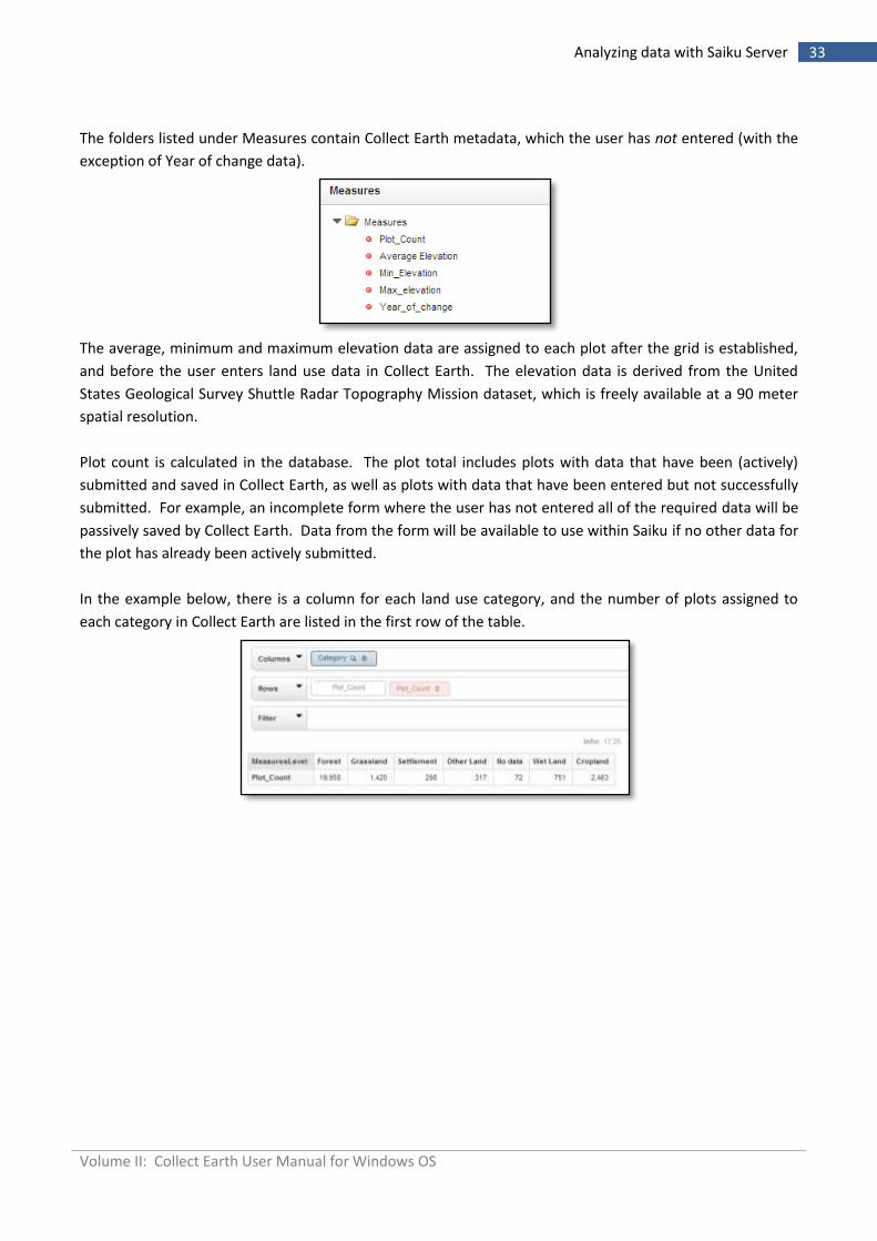
The folders listed under Measures contain Collect Earth metadata, which the user has not entered (with the
exception of Year of change data).
The average, minimum and maximum elevation data are assigned to each plot after the grid is established,
and before the user enters land use data in Collect Earth. The elevation data is derived from the United
States Geological Survey Shuttle Radar Topography Mission dataset, which is freely available at a 90 meter
spatial resolution.
Plot count is calculated in the database. The plot total includes plots with data that have been (actively)
submitted and saved in Collect Earth, as well as plots with data that have been entered but not successfully
submitted. For example, an incomplete form where the user has not entered all of the required data will be
passively saved by Collect Earth. Data from the form will be available to use within Saiku if no other data for
the plot has already been actively submitted.
In the example below, there is a column for each land use category, and the number of plots assigned to
each category in Collect Earth are listed in the first row of the table.
Volume II: Collect Earth User Manual for Windows OS
34 Analyzing data with Saiku Server
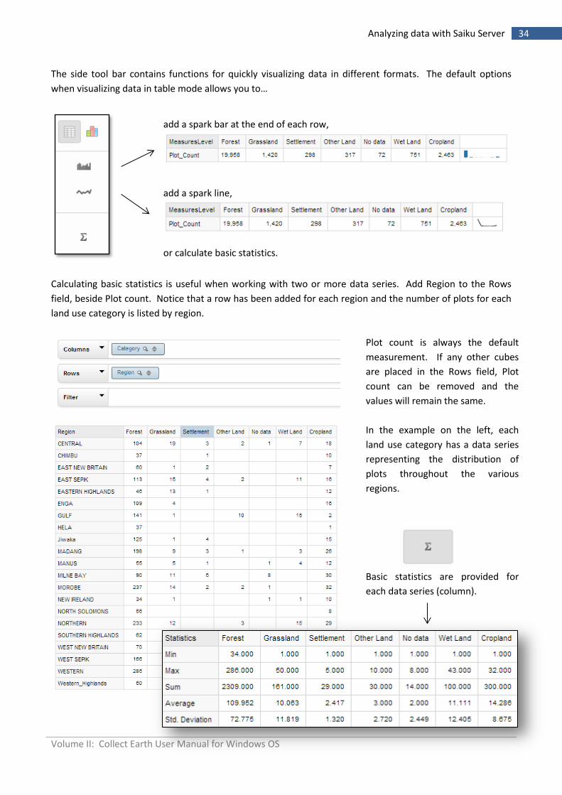
The side tool bar contains functions for quickly visualizing data in different formats. The default options
when visualizing data in table mode allows you to…
add a spark bar at the end of each row,
add a spark line,
or calculate basic statistics.
Calculating basic statistics is useful when working with two or more data series. Add Region to the Rows
field, beside Plot count. Notice that a row has been added for each region and the number of plots for each
land use category is listed by region.
Plot count is always the default
measurement. If any other cubes
are placed in the Rows field, Plot
count can be removed and the
values will remain the same.
In the example on the left, each
land use category has a data series
representing the distribution of
plots throughout the various
regions.
Basic statistics are provided for
each data series (column).
Volume II: Collect Earth User Manual for Windows OS
35 Analyzing data with Saiku Server
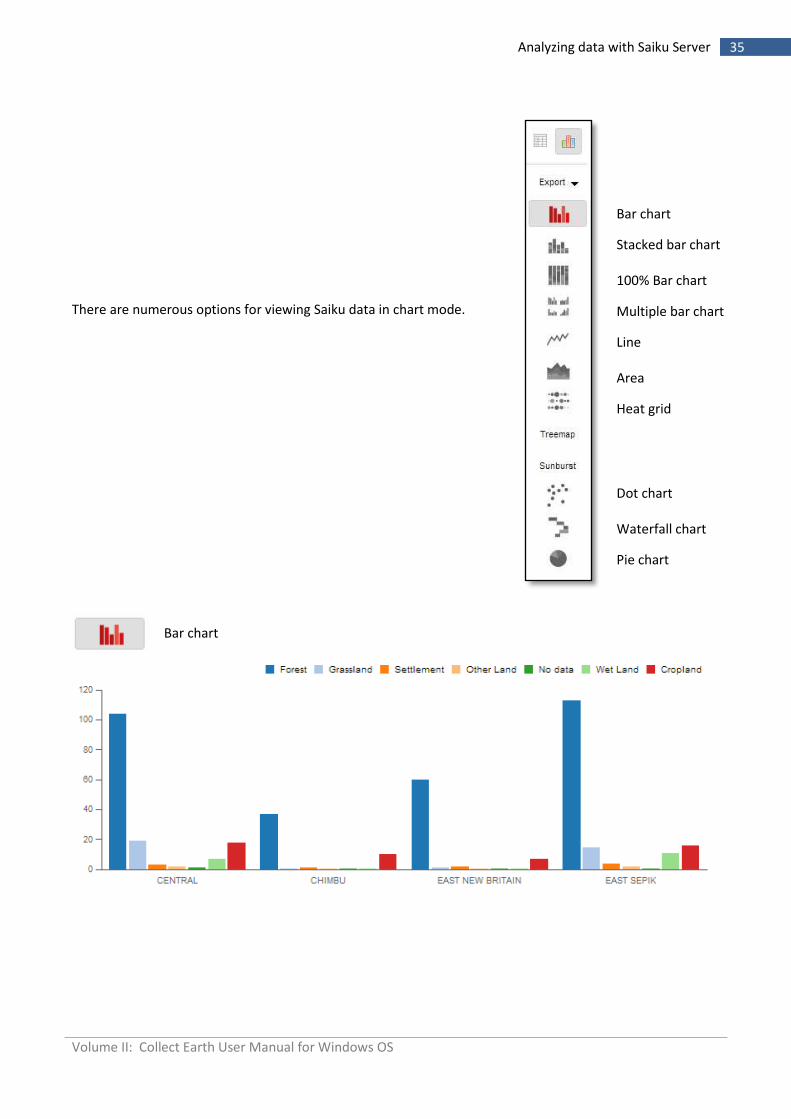
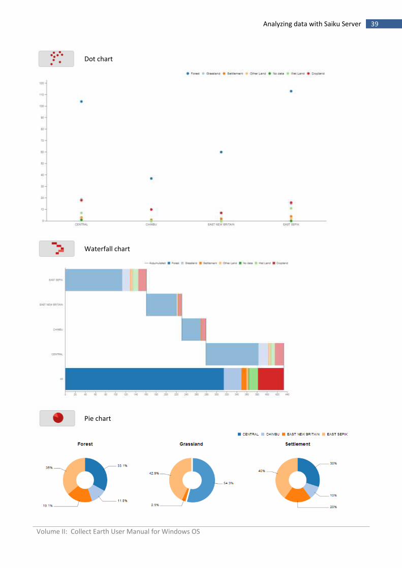
There are numerous options for viewing Saiku data in chart mode.
Bar chart
Stacked bar chart 100% Bar chart
Multiple bar chart
Line Area
Heat grid
Dot chart Waterfall chart
Pie chart
Bar chart
Volume II: Collect Earth User Manual for Windows OS
36 Analyzing data with Saiku Server
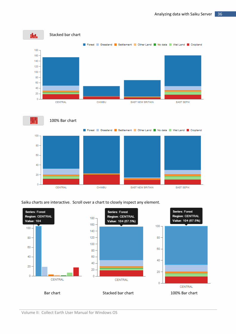
Stacked bar chart
100% Bar chart
Saiku charts are interactive. Scroll over a chart to closely inspect any element.
Bar chart Stacked bar chart 100% Bar chart
Volume II: Collect Earth User Manual for Windows OS
37 Analyzing data with Saiku Server
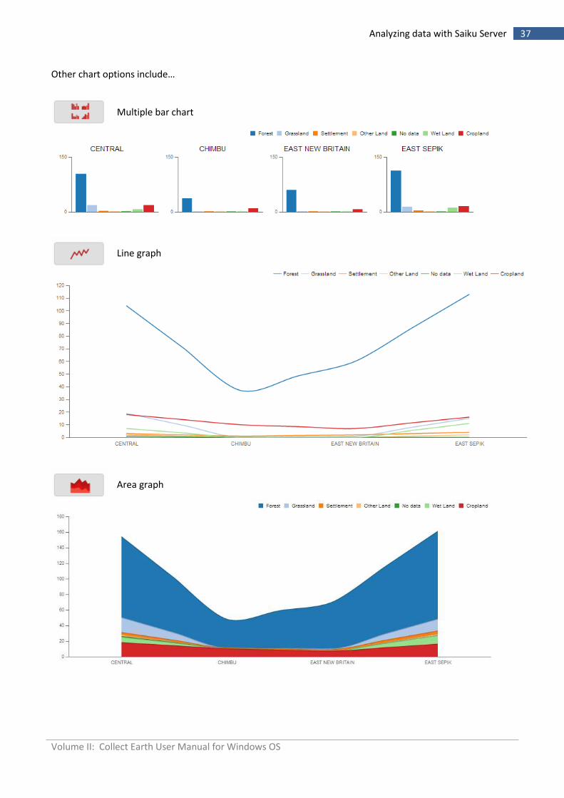
Other chart options include…
Multiple bar chart
Line graph
Area graph
Volume II: Collect Earth User Manual for Windows OS
38 Analyzing data with Saiku Server
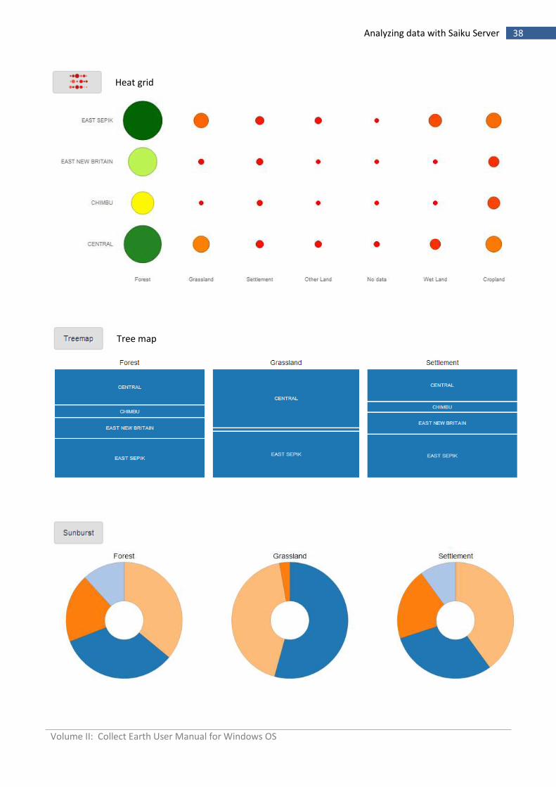
Heat grid
Tree map
Volume II: Collect Earth User Manual for Windows OS
39 Analyzing data with Saiku Server
Dot chart
Waterfall chart
Pie chart
Volume II: Collect Earth User Manual for Windows OS
40 Analyzing data with Saiku Server
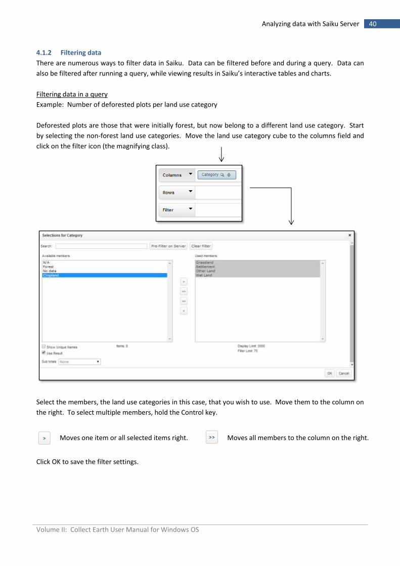
4.1.2 Filtering data
There are numerous ways to filter data in Saiku. Data can be filtered before and during a query. Data can
also be filtered after running a query, while viewing results in Saiku’s interactive tables and charts.
Filtering data in a query
Example: Number of deforested plots per land use category
Deforested plots are those that were initially forest, but now belong to a different land use category. Start
by selecting the non-forest land use categories. Move the land use category cube to the columns field and
click on the filter icon (the magnifying class).
Select the members, the land use categories in this case, that you wish to use. Move them to the column on
the right. To select multiple members, hold the Control key.
Moves one item or all selected items right.
Moves all members to the column on the right.
Click OK to save the filter settings.
Volume II: Collect Earth User Manual for Windows OS
41 Analyzing data with Saiku Server
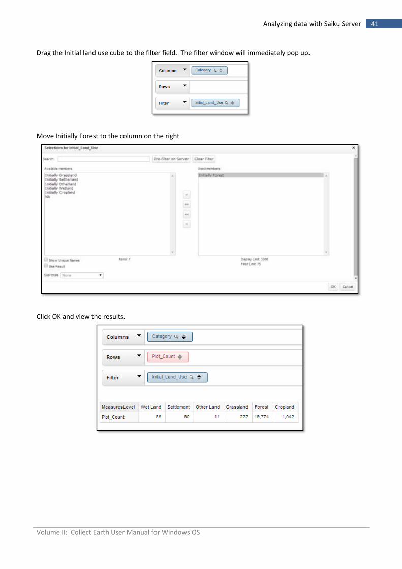
Drag the Initial land use cube to the filter field. The filter window will immediately pop up.
Move Initially Forest to the column on the right
Click OK and view the results.
Volume II: Collect Earth User Manual for Windows OS
42 Analyzing data with Saiku Server
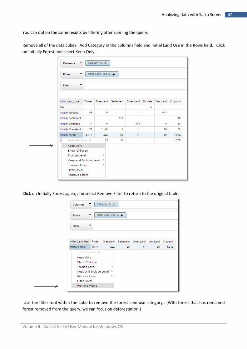
You can obtain the same results by filtering after running the query.
Remove all of the data cubes. Add Category in the columns field and Initial Land Use in the Rows field. Click
on Initially Forest and select Keep Only.
Click on Initially Forest again, and select Remove Filter to return to the original table.
Use the filter tool within the cube to remove the forest land use category. (With forest that has remained
forest removed from the query, we can focus on deforestation.)
Volume II: Collect Earth User Manual for Windows OS
43 Analyzing data with Saiku Server
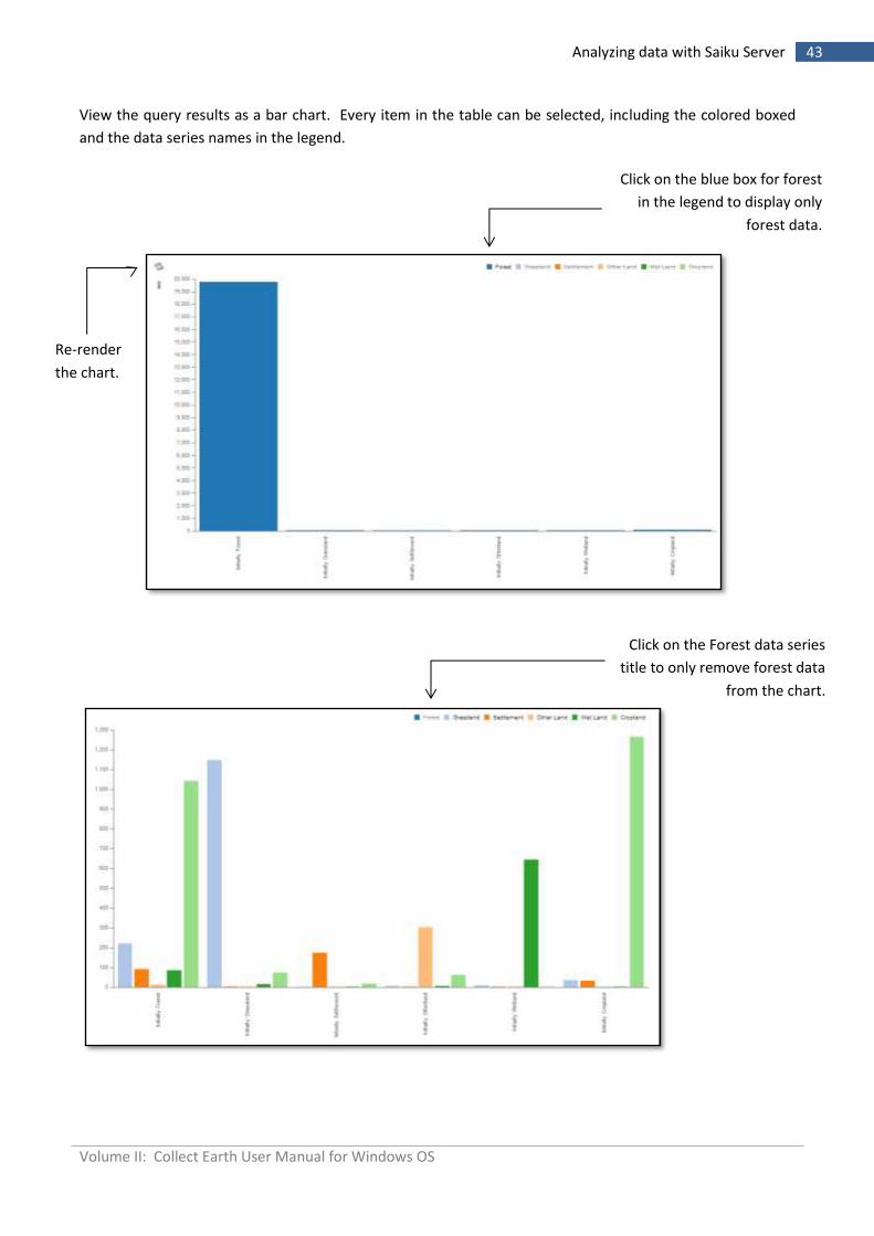
View the query results as a bar chart. Every item in the table can be selected, including the colored boxed
and the data series names in the legend.
Click on the blue box for forest
in the legend to display only
forest data.
Re-render
the chart.
Click on the Forest data series
title to only remove forest data
from the chart.
Volume II: Collect Earth User Manual for Windows OS
44 Analyzing data with Saiku Server
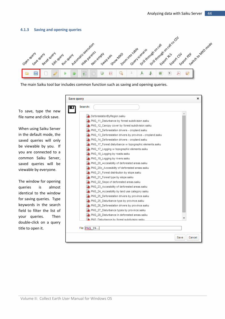
4.1.3 Saving and opening queries
The main Saiku tool bar includes common function such as saving and opening queries.
Open qu
ery
Save
query
Reset q
uery
Edit
query
Run query
Autom
atic
execu
tion
Hide p
aren
ts
Non-em
pty
Swap a
xis
Show M
XD
Zoom
into
table
Query s
cenar
io
Drill t
hrough
on ce
ll
Drill t
hrough
on ce
ll to CS
V
Export
XLS
Export
CSV
Export
Switc
h to M
XD mode
To save, type the new
file name and click save.
When using Saiku Server
in the default mode, the
saved queries will only
be viewable by you. If
you are connected to a
common Saiku Server,
saved queries will be
viewable by everyone.
The window for opening
queries is almost
identical to the window
for saving queries. Type
keywords in the search
field to filter the list of
your queries. Then
double-click on a query
title to open it.
Volume II: Collect Earth User Manual for Windows OS
45 Analyzing data with Saiku Server
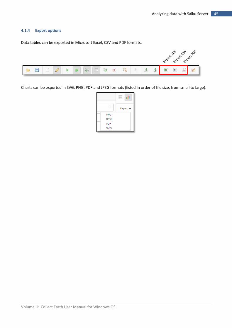
4.1.4 Export options
Data tables can be exported in Microsoft Excel, CSV and PDF formats.
Charts can be exported in SVG, PNG, PDF and JPEG formats (listed in order of file size, from small to large).
Open qu
ery
Save
query
Reset q
uery
Edit
query
Run query
Autom
atic
execu
tion
Hide p
aren
ts
Non-em
pty
Swap a
xis
Show M
XD
Zoom
into
table
Query s
cenar
io
Drill t
hrough
on ce
ll
Drill t
hrough
on ce
ll to CS
V
Export
XLS
Export
CSV
Export
Switc
h to M
XD mode
Volume II: Collect Earth User Manual for Windows OS
46 Analyzing data with Saiku Server
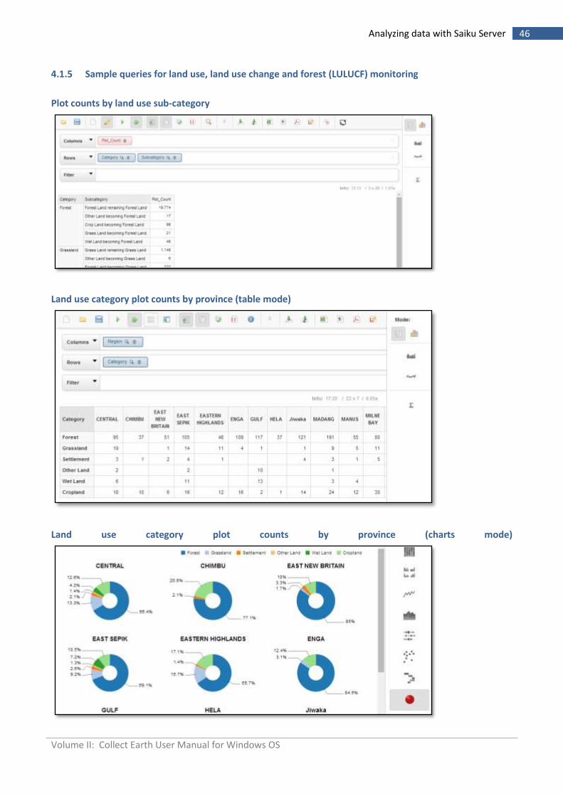
4.1.5 Sample queries for land use, land use change and forest (LULUCF) monitoring
Plot counts by land use sub-category
Land use category plot counts by province (table mode)
Land use category plot counts by province (charts mode)
Volume II: Collect Earth User Manual for Windows OS
47 Analyzing data with Saiku Server
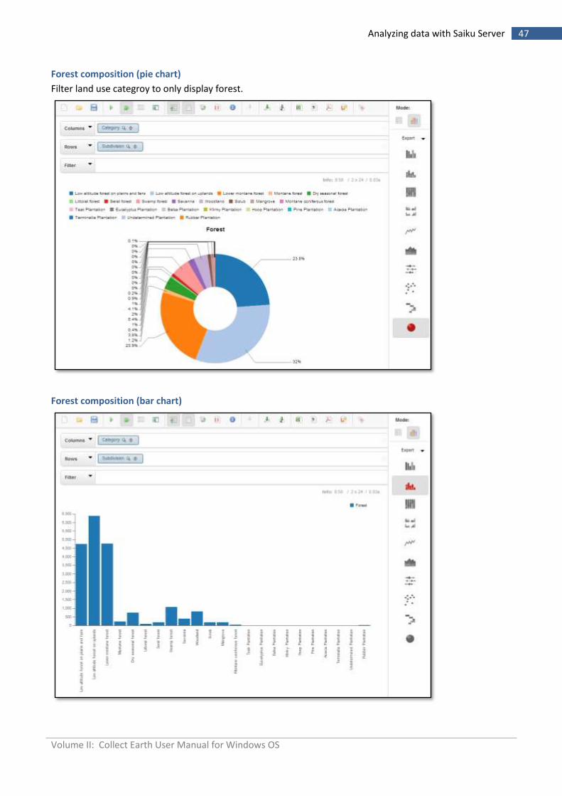
Forest composition (pie chart)
Filter land use categroy to only display forest.
Forest composition (bar chart)
Volume II: Collect Earth User Manual for Windows OS
48 Analyzing data with Saiku Server
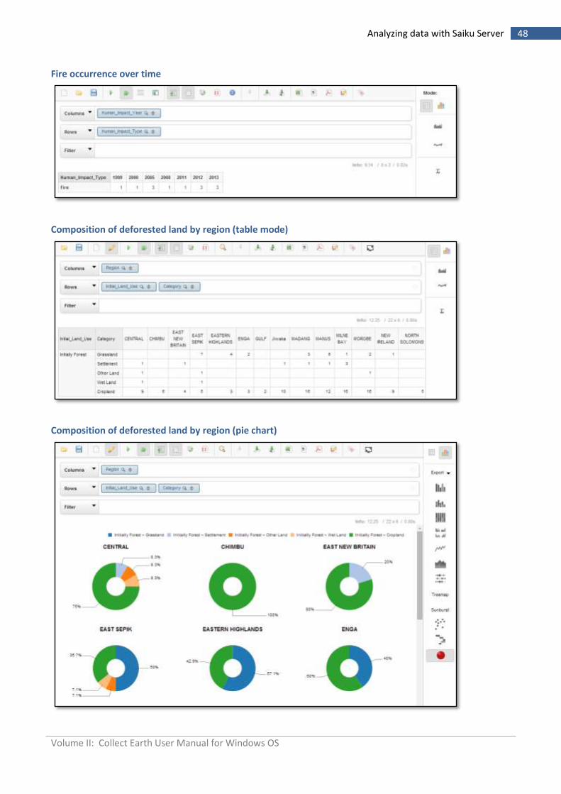
Fire occurrence over time
Composition of deforested land by region (table mode)
Composition of deforested land by region (pie chart)
Volume II: Collect Earth User Manual for Windows OS
49 Analyzing data with Saiku Server
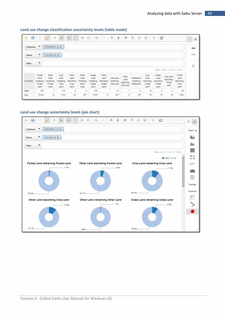
Land use change classification uncertainty levels (table mode)
Land use change uncertainty levels (pie chart)
Volume II: Collect Earth User Manual for Windows OS
50 Processing geospatial data with QGIS
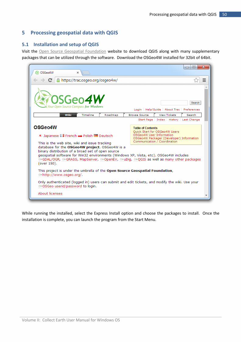
5 Processing geospatial data with QGIS
5.1 Installation and setup of QGIS
Visit the Open Source Geospatial Foundation website to download QGIS along with many supplementary
packages that can be utilized through the software. Download the OSGeo4W installed for 32bit of 64bit.
While running the installed, select the Express Install option and choose the packages to install. Once the
installation is complete, you can launch the program from the Start Menu.
Volume II: Collect Earth User Manual for Windows OS
51 Processing geospatial data with QGIS
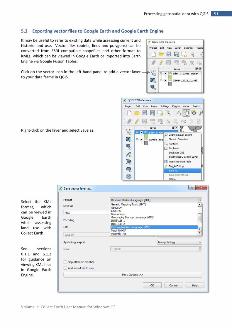
5.2 Exporting vector files to Google Earth and Google Earth Engine
It may be useful to refer to existing data while assessing current and historic land use. Vector files (points, lines and polygons) can be converted from ESRI compatible shapefiles and other format to KMLs, which can be viewed in Google Earth or imported into Earth Engine via Google Fusion Tables. Click on the vector icon in the left-hand panel to add a vector layer to your data frame in QGIS.
Right-click on the layer and select Save as.
Select the KML format, which can be viewed in Google Earth while assessing land use with Collect Earth. See sections 6.1.1 and 6.1.2 for guidance on viewing KML files in Google Earth Engine.
Volume II: Collect Earth User Manual for Windows OS
52 Processing geospatial data with QGIS
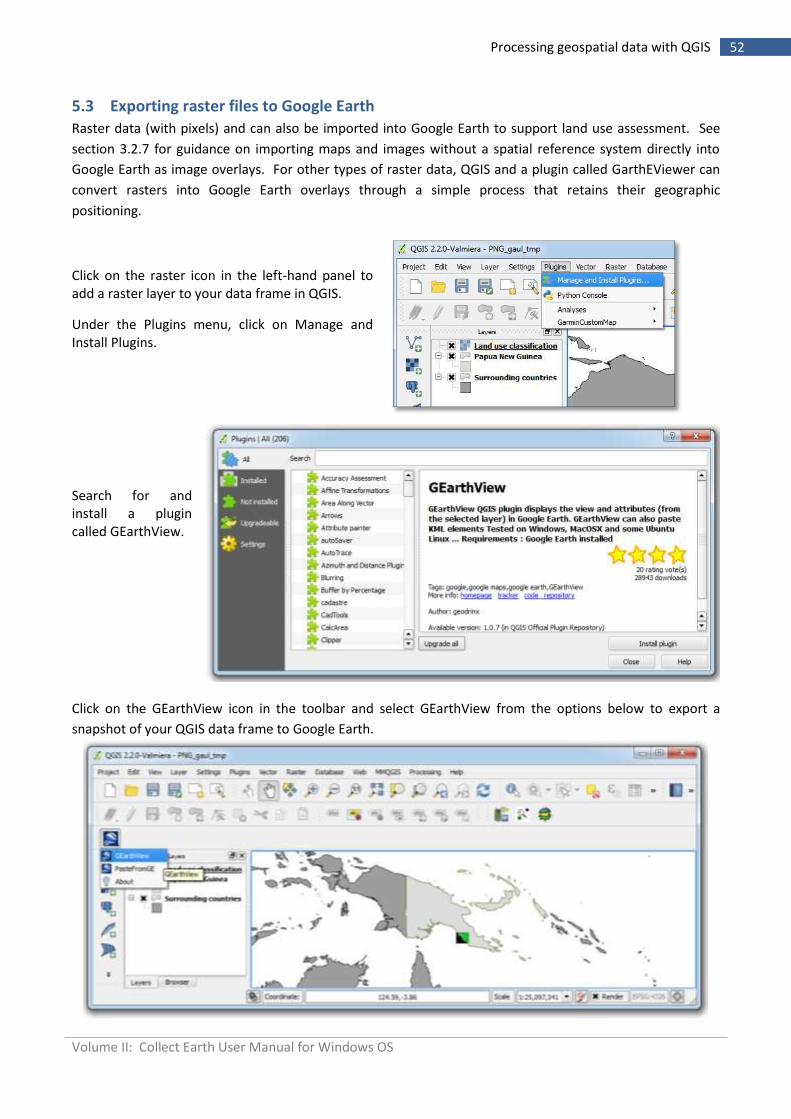
5.3 Exporting raster files to Google Earth
Raster data (with pixels) and can also be imported into Google Earth to support land use assessment. See
section 3.2.7 for guidance on importing maps and images without a spatial reference system directly into
Google Earth as image overlays. For other types of raster data, QGIS and a plugin called GarthEViewer can
convert rasters into Google Earth overlays through a simple process that retains their geographic
positioning.
Click on the raster icon in the left-hand panel to add a raster layer to your data frame in QGIS.
Under the Plugins menu, click on Manage and Install Plugins.
Search for and install a plugin called GEarthView.
Click on the GEarthView icon in the toolbar and select GEarthView from the options below to export a
snapshot of your QGIS data frame to Google Earth.
Volume II: Collect Earth User Manual for Windows OS
53 Processing geospatial data with QGIS
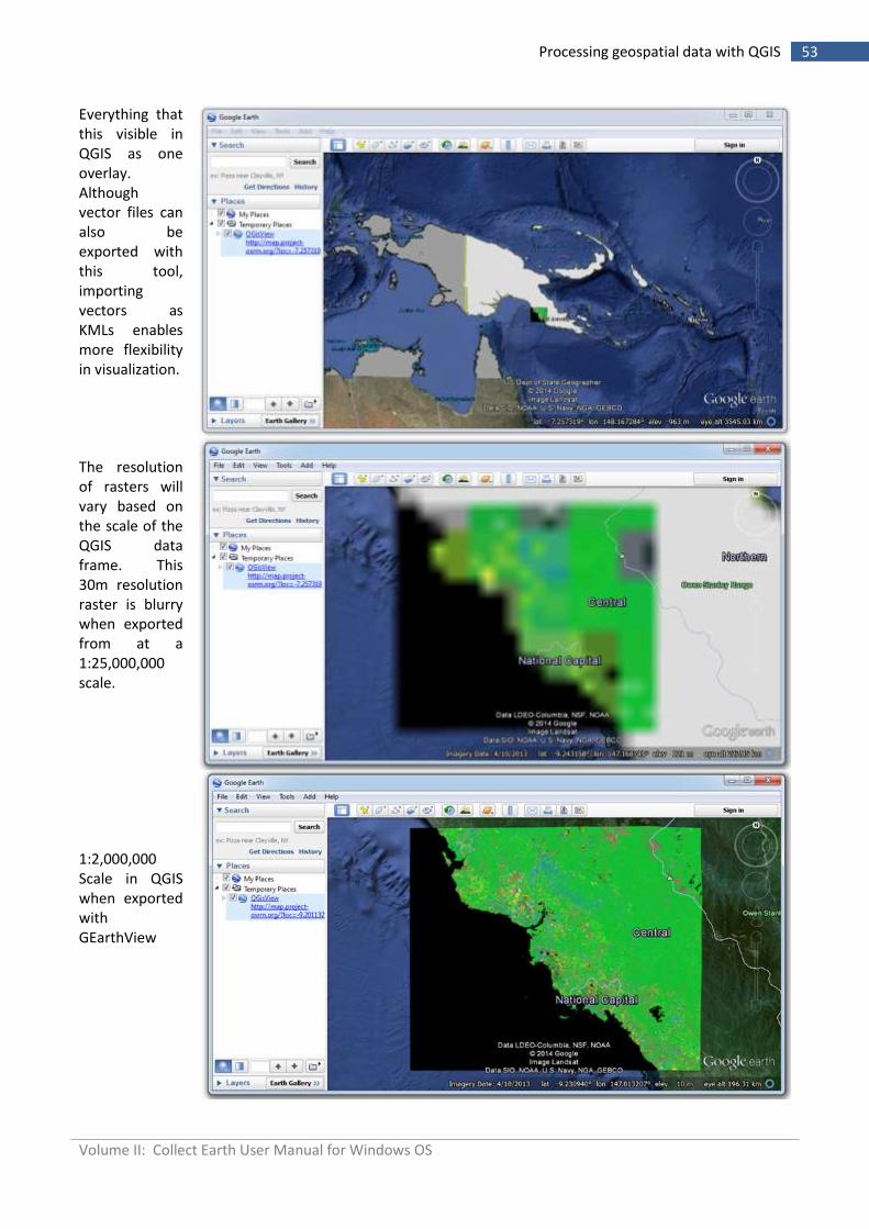
Everything that this visible in QGIS as one overlay. Although vector files can also be exported with this tool, importing vectors as KMLs enables more flexibility in visualization.
The resolution of rasters will vary based on the scale of the QGIS data frame. This 30m resolution raster is blurry when exported from at a 1:25,000,000 scale.
1:2,000,000 Scale in QGIS when exported with GEarthView
Volume II: Collect Earth User Manual for Windows OS
54 Processing geospatial data with QGIS
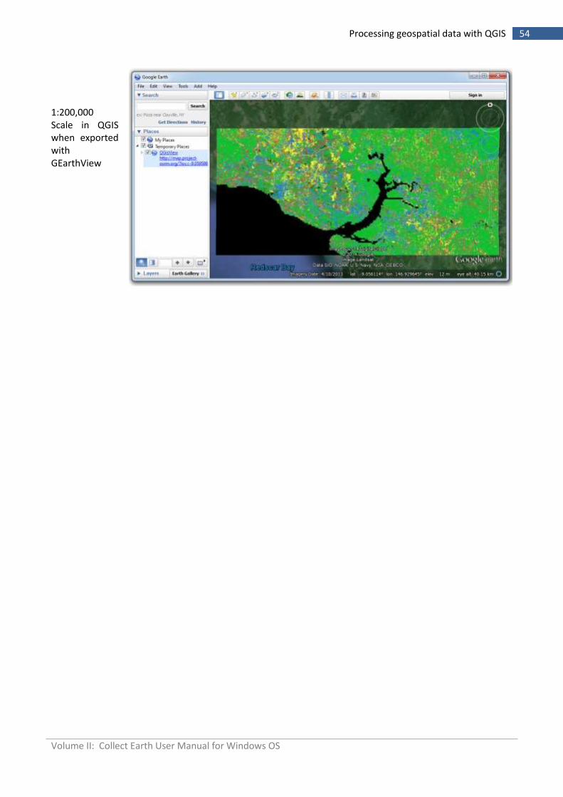
1:200,000 Scale in QGIS when exported with GEarthView
Volume II: Collect Earth User Manual for Windows OS
55 Processing geospatial data with QGIS
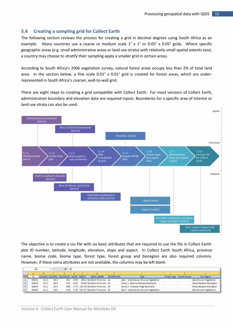
5.4 Creating a sampling grid for Collect Earth
The following section reviews the process for creating a grid in decimal degrees using South Africa as an
example. Many countries use a coarse or medium scale 1° x 1° or 0.05° x 0.05° grids. Where specific
geographic areas (e.g. small administrative areas or land use strata) with relatively small spatial extents exist,
a country may choose to stratify their sampling apply a smaller grid in certain areas.
According to South Africa’s 2006 vegetation survey, natural forest areas occupy less than 2% of total land
area. In the section below, a fine scale 0.01° x 0.01° grid is created for forest areas, which are under-
represented in South Africa’s coarser, wall-to-wall grid.
There are eight steps to creating a grid compatible with Collect Earth. For most versions of Collect Earth,
administration boundary and elevation data are required inputs. Boundaries for a specific area of interest or
land use strata can also be used.
The objective is to create a csv file with six basic attributes that are required to use the file in Collect Earth:
plot ID number, latitude, longitude, elevation, slope and aspect. In Collect Earth South Africa, province
name, biome code, biome type, forest type, forest group and bioregion are also required columns.
However, if these extra attributes are not available, the columns may be left blank.
Volume II: Collect Earth User Manual for Windows OS
56 Processing geospatial data with QGIS
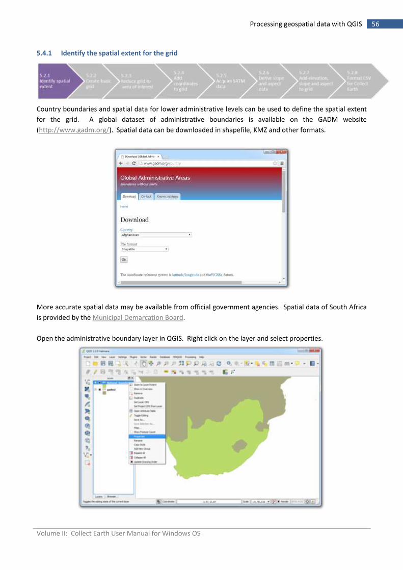
5.4.1 Identify the spatial extent for the grid
Country boundaries and spatial data for lower administrative levels can be used to define the spatial extent
for the grid. A global dataset of administrative boundaries is available on the GADM website
(http://www.gadm.org/). Spatial data can be downloaded in shapefile, KMZ and other formats.
More accurate spatial data may be available from official government agencies. Spatial data of South Africa
is provided by the Municipal Demarcation Board.
Open the administrative boundary layer in QGIS. Right click on the layer and select properties.
Volume II: Collect Earth User Manual for Windows OS
57 Processing geospatial data with QGIS
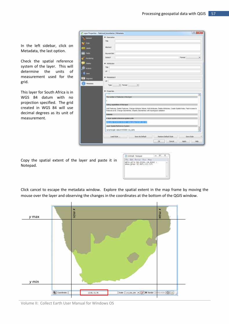
In the left sidebar, click on Metadata, the last option. Check the spatial reference system of the layer. This will determine the units of measurement used for the grid. This layer for South Africa is in WGS 84 datum with no projection specified. The grid created in WGS 84 will use decimal degrees as its unit of measurement.
Copy the spatial extent of the layer and paste it in Notepad.
Click cancel to escape the metadata window. Explore the spatial extent in the map frame by moving the
mouse over the layer and observing the changes in the coordinates at the bottom of the QGIS window.
y max
y min
x min
x max
Volume II: Collect Earth User Manual for Windows OS
58 Processing geospatial data with QGIS
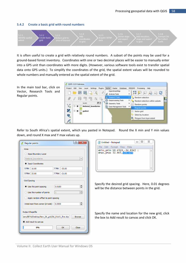
5.4.2 Create a basic grid with round numbers
It is often useful to create a grid with relatively round numbers. A subset of the points may be used for a
ground-based forest inventory. Coordinates with one or two decimal places will be easier to manually enter
into a GPS unit than coordinates with more digits. (However, various software tools exist to transfer spatial
data onto GPS units.) To simplify the coordinates of the grid, the spatial extent values will be rounded to
whole numbers and manually entered as the spatial extent of the grid.
In the main tool bar, click on Vector, Research Tools and Regular points.
Refer to South Africa’s spatial extent, which you pasted in Notepad. Round the X min and Y min values
down, and round X max and Y max values up.
Specify the desired grid spacing. Here, 0.01 degrees will be the distance between points in the grid. Specify the name and location for the new grid, click the box to Add result to canvas and click OK.
Volume II: Collect Earth User Manual for Windows OS
59 Processing geospatial data with QGIS
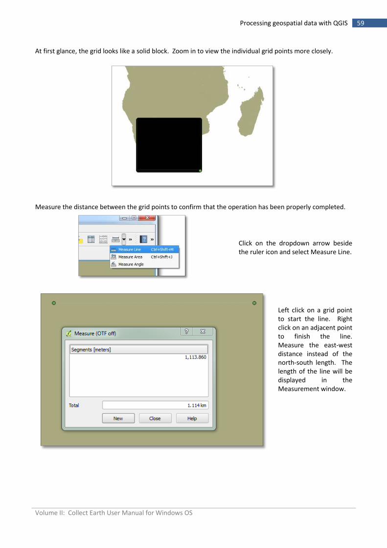
At first glance, the grid looks like a solid block. Zoom in to view the individual grid points more closely.
Measure the distance between the grid points to confirm that the operation has been properly completed.
Click on the dropdown arrow beside the ruler icon and select Measure Line.
Left click on a grid point to start the line. Right click on an adjacent point to finish the line. Measure the east-west distance instead of the north-south length. The length of the line will be displayed in the Measurement window.
Volume II: Collect Earth User Manual for Windows OS
60 Processing geospatial data with QGIS
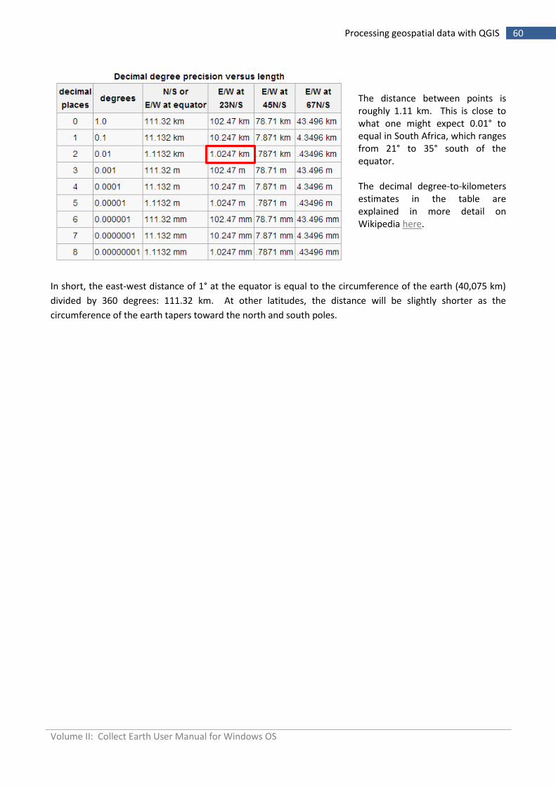
The distance between points is roughly 1.11 km. This is close to what one might expect 0.01° to equal in South Africa, which ranges from 21° to 35° south of the equator. The decimal degree-to-kilometers estimates in the table are explained in more detail on Wikipedia here.
In short, the east-west distance of 1° at the equator is equal to the circumference of the earth (40,075 km)
divided by 360 degrees: 111.32 km. At other latitudes, the distance will be slightly shorter as the
circumference of the earth tapers toward the north and south poles.
Volume II: Collect Earth User Manual for Windows OS
61 Processing geospatial data with QGIS
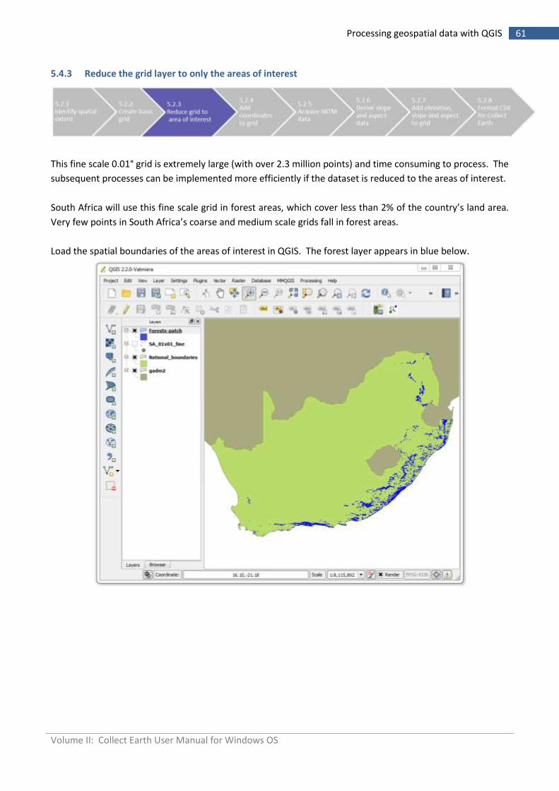
5.4.3 Reduce the grid layer to only the areas of interest
This fine scale 0.01° grid is extremely large (with over 2.3 million points) and time consuming to process. The
subsequent processes can be implemented more efficiently if the dataset is reduced to the areas of interest.
South Africa will use this fine scale grid in forest areas, which cover less than 2% of the country’s land area.
Very few points in South Africa’s coarse and medium scale grids fall in forest areas.
Load the spatial boundaries of the areas of interest in QGIS. The forest layer appears in blue below.
Volume II: Collect Earth User Manual for Windows OS
62 Processing geospatial data with QGIS
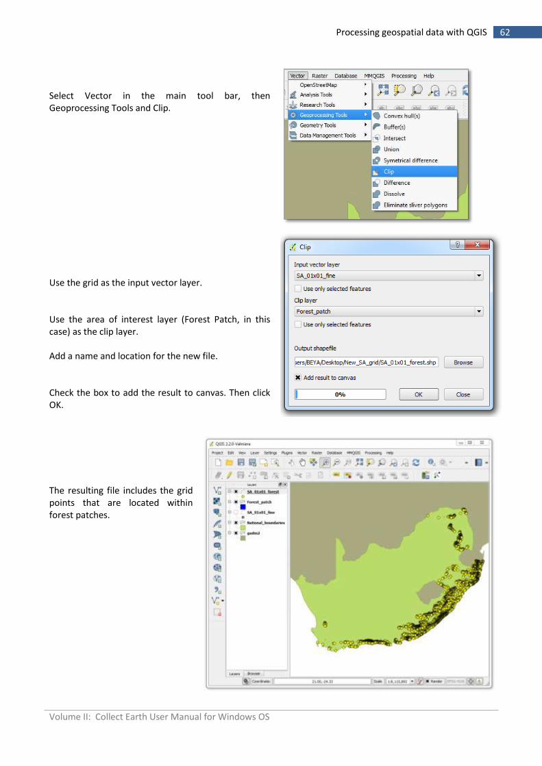
Select Vector in the main tool bar, then Geoprocessing Tools and Clip.
Use the grid as the input vector layer. Use the area of interest layer (Forest Patch, in this case) as the clip layer. Add a name and location for the new file. Check the box to add the result to canvas. Then click OK.
The resulting file includes the grid points that are located within forest patches.
Volume II: Collect Earth User Manual for Windows OS
63 Processing geospatial data with QGIS
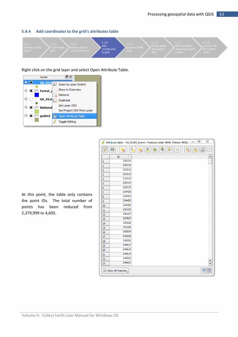
5.4.4 Add coordinates to the grid’s attributes table
Right click on the grid layer and select Open Attribute Table.
At this point, the table only contains
the point IDs. The total number of
points has been reduced from
2,379,999 to 4,605.
Volume II: Collect Earth User Manual for Windows OS
64 Processing geospatial data with QGIS
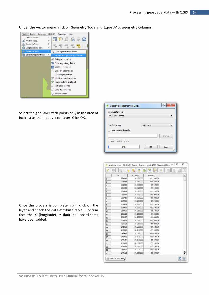
Under the Vector menu, click on Geometry Tools and Export/Add geometry columns.
Select the grid layer with points only in the area of interest as the Input vector layer. Click OK.
Once the process is complete, right click on the layer and check the data attribute table. Confirm that the X (longitude), Y (latitude) coordinates have been added.
Volume II: Collect Earth User Manual for Windows OS
65 Processing geospatial data with QGIS
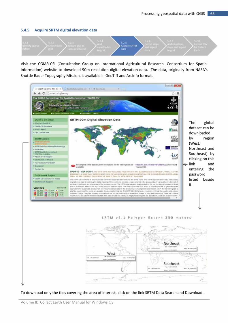
5.4.5 Acquire SRTM digital elevation data
Visit the CGIAR-CSI (Consultative Group on International Agricultural Research, Consortium for Spatial
Information) website to download 90m resolution digital elevation data. The data, originally from NASA’s
Shuttle Radar Topography Mission, is available in GeoTiff and ArcInfo format.
The global dataset can be downloaded by region (West, Northeast and Southeast) by clicking on this link and entering the password listed beside it.
To download only the tiles covering the area of interest, click on the link SRTM Data Search and Download.
Volume II: Collect Earth User Manual for Windows OS
66 Processing geospatial data with QGIS
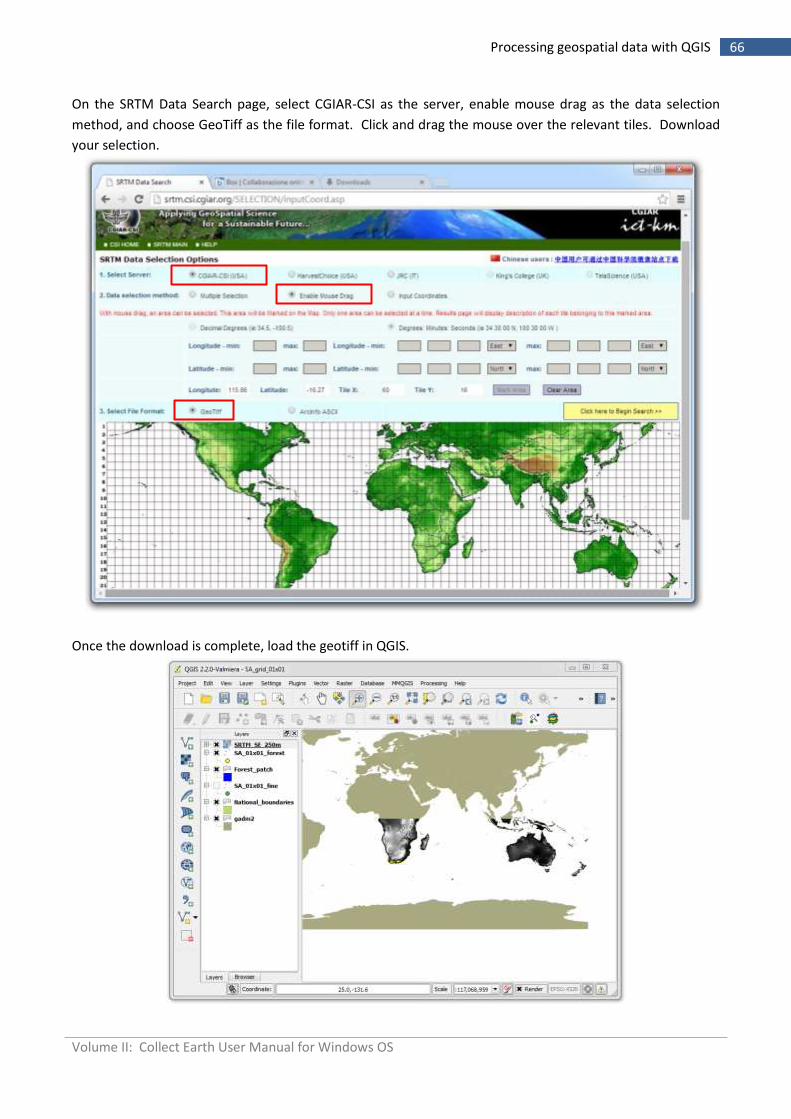
On the SRTM Data Search page, select CGIAR-CSI as the server, enable mouse drag as the data selection
method, and choose GeoTiff as the file format. Click and drag the mouse over the relevant tiles. Download
your selection.
Once the download is complete, load the geotiff in QGIS.
Volume II: Collect Earth User Manual for Windows OS
67 Processing geospatial data with QGIS
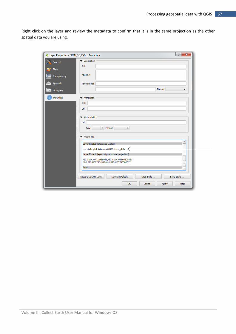
Right click on the layer and review the metadata to confirm that it is in the same projection as the other
spatial data you are using.
Volume II: Collect Earth User Manual for Windows OS
68 Processing geospatial data with QGIS
5.4.6 Derive slope and aspect data from digital elevation data
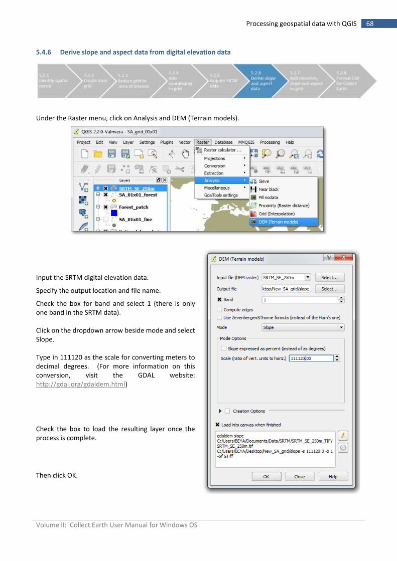
Under the Raster menu, click on Analysis and DEM (Terrain models).
Input the SRTM digital elevation data.
Specify the output location and file name.
Check the box for band and select 1 (there is only one band in the SRTM data). Click on the dropdown arrow beside mode and select Slope. Type in 111120 as the scale for converting meters to decimal degrees. (For more information on this conversion, visit the GDAL website: http://gdal.org/gdaldem.html) Check the box to load the resulting layer once the process is complete.
Then click OK.
Volume II: Collect Earth User Manual for Windows OS
69 Processing geospatial data with QGIS
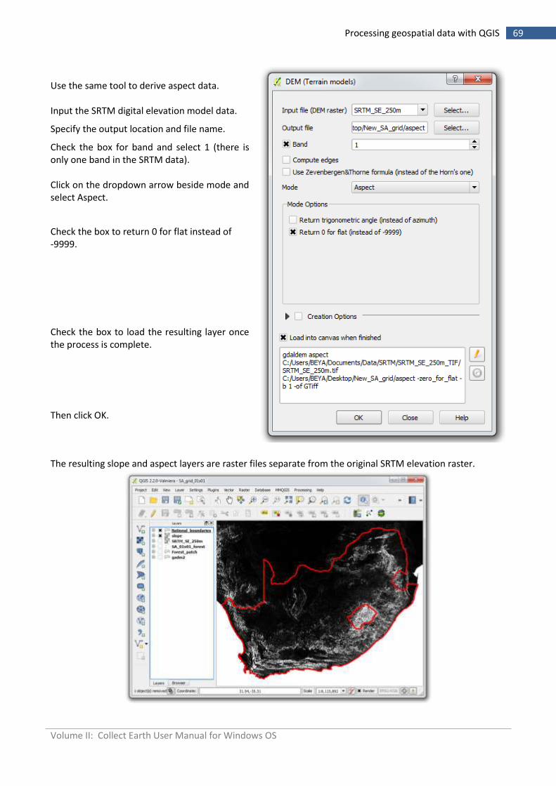
Use the same tool to derive aspect data. Input the SRTM digital elevation model data.
Specify the output location and file name.
Check the box for band and select 1 (there is only one band in the SRTM data). Click on the dropdown arrow beside mode and select Aspect.
Check the box to return 0 for flat instead of -9999. Check the box to load the resulting layer once the process is complete.
Then click OK.
The resulting slope and aspect layers are raster files separate from the original SRTM elevation raster.
Volume II: Collect Earth User Manual for Windows OS
70 Processing geospatial data with QGIS
5.4.7 Add elevation, slope and aspect data to the grid
There are two parts to this step. In the first part, elevation, slope and aspect data are extracted from the
rasters and associated with each point in the forest grid. This results in three separate point files. The
second part involves consolidating the elevation, slope and aspect data into the main forest grid file, which
already contains the point coordinates.
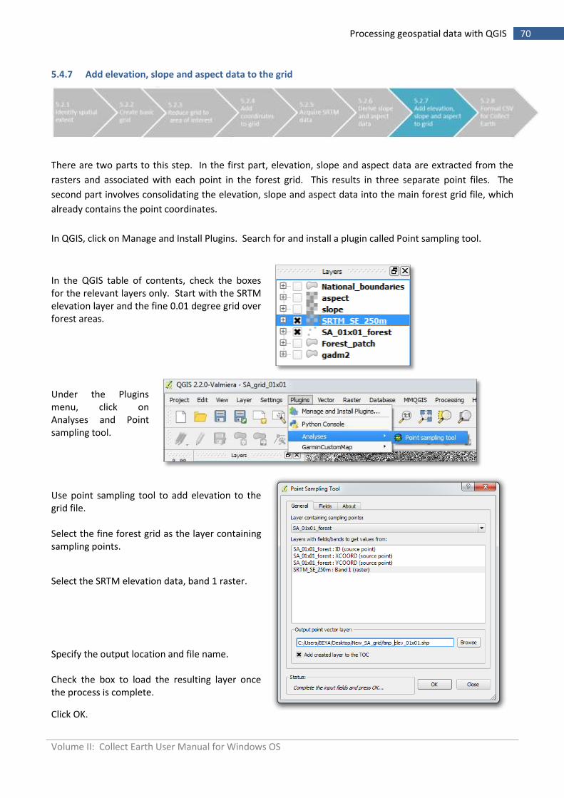
In QGIS, click on Manage and Install Plugins. Search for and install a plugin called Point sampling tool.
In the QGIS table of contents, check the boxes for the relevant layers only. Start with the SRTM elevation layer and the fine 0.01 degree grid over forest areas.
Under the Plugins menu, click on Analyses and Point sampling tool.
Use point sampling tool to add elevation to the grid file. Select the fine forest grid as the layer containing sampling points.
Select the SRTM elevation data, band 1 raster.
Specify the output location and file name. Check the box to load the resulting layer once the process is complete.
Click OK.
Volume II: Collect Earth User Manual for Windows OS
71 Processing geospatial data with QGIS
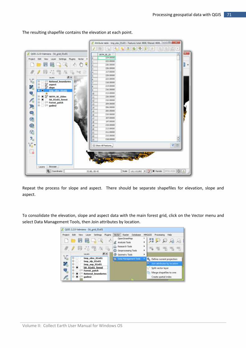
The resulting shapefile contains the elevation at each point.
Repeat the process for slope and aspect. There should be separate shapefiles for elevation, slope and
aspect.
To consolidate the elevation, slope and aspect data with the main forest grid, click on the Vector menu and
select Data Management Tools, then Join attributes by location.
Volume II: Collect Earth User Manual for Windows OS
72 Processing geospatial data with QGIS
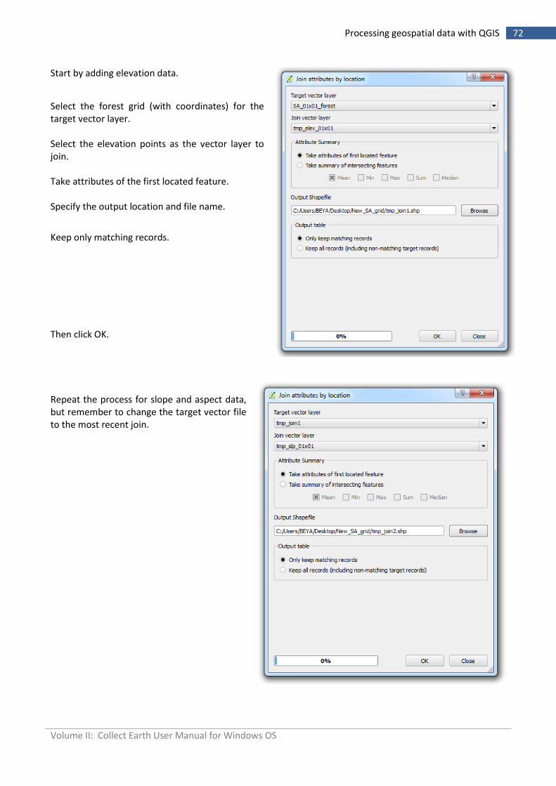
Start by adding elevation data.
Select the forest grid (with coordinates) for the target vector layer. Select the elevation points as the vector layer to join. Take attributes of the first located feature. Specify the output location and file name.
Keep only matching records.
Then click OK.
Repeat the process for slope and aspect data, but remember to change the target vector file to the most recent join.
Volume II: Collect Earth User Manual for Windows OS
73 Processing geospatial data with QGIS
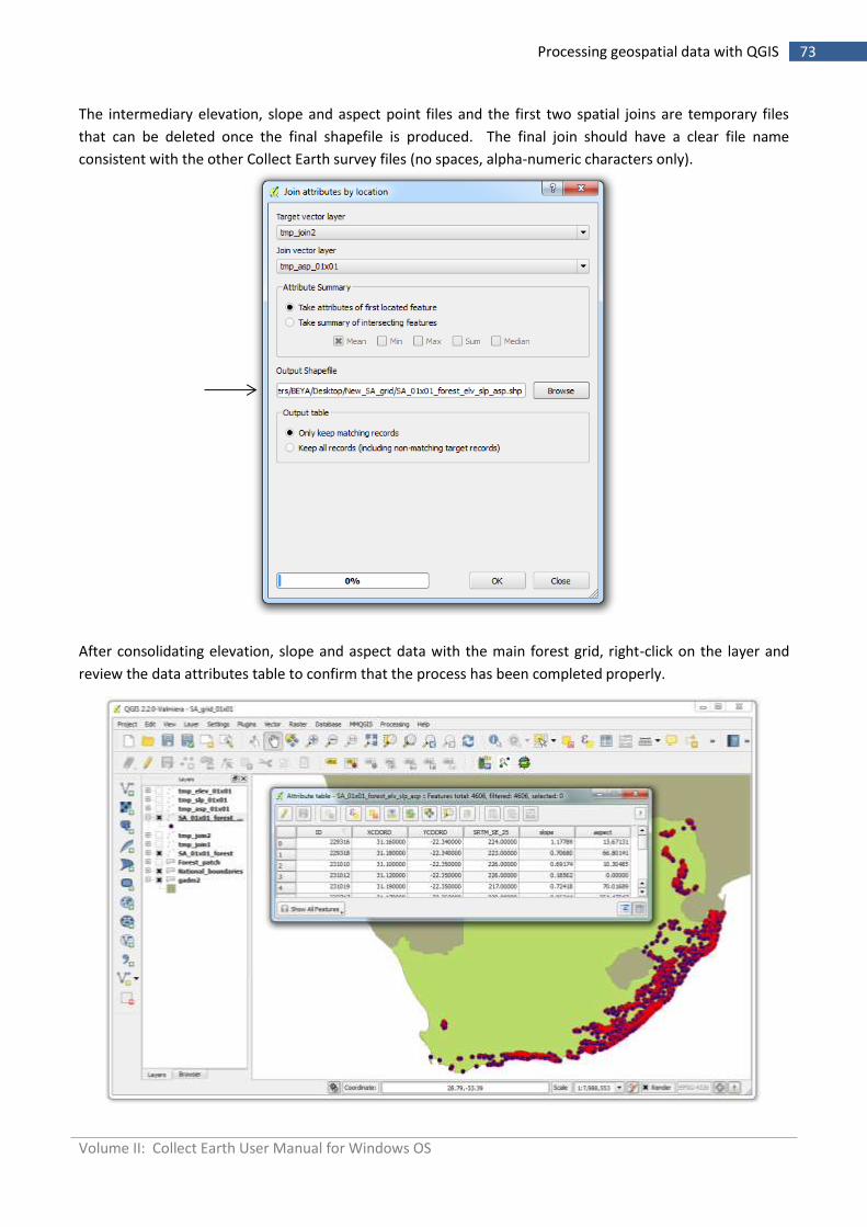
The intermediary elevation, slope and aspect point files and the first two spatial joins are temporary files
that can be deleted once the final shapefile is produced. The final join should have a clear file name
consistent with the other Collect Earth survey files (no spaces, alpha-numeric characters only).
After consolidating elevation, slope and aspect data with the main forest grid, right-click on the layer and
review the data attributes table to confirm that the process has been completed properly.
Volume II: Collect Earth User Manual for Windows OS
74 Processing geospatial data with QGIS
5.4.8 Format the grid as a CSV compatible with Collect Earth
Collect Earth uses grids in csv format with six basic attributes in a particular order:
plot ID number
latitude (y coordinate)
longitude (x coordinate)
elevation
slope
aspect
Collect Earth South Africa draws upon several additional attributes. Again, the order of the columns is
important for compatibility, but the columns can be empty if such data is not available or up-to-date:
ADM1_NAME (province name)
BIOMECODE
Type
Forest Type
Forest Group
Bio Region
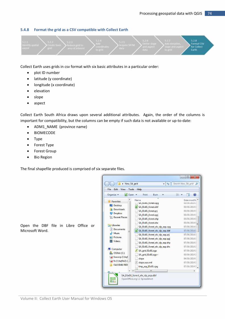
The final shapefile produced is comprised of six separate files.
Open the DBF file in Libre Office or Microsoft Word.
Volume II: Collect Earth User Manual for Windows OS
75 Processing geospatial data with QGIS
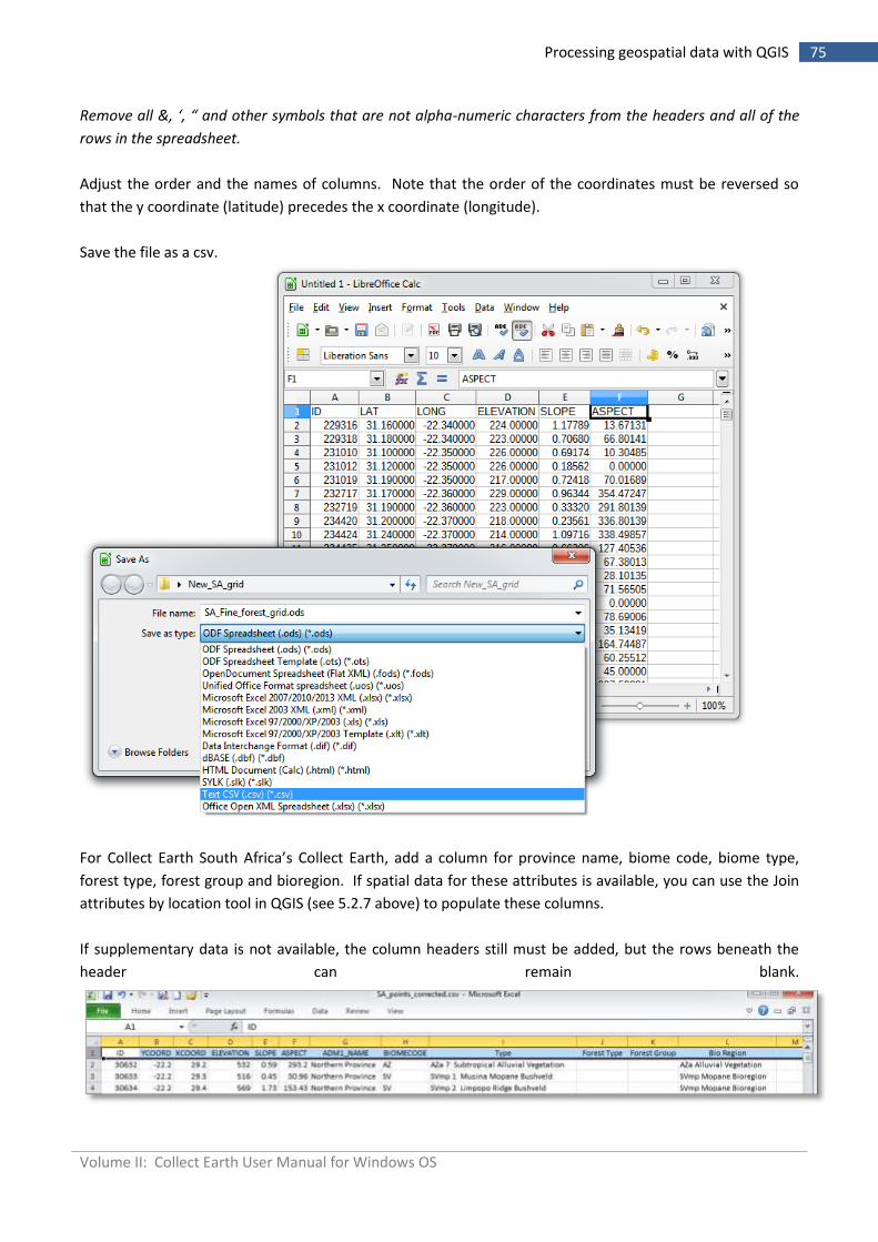
Remove all &, ‘, “ and other symbols that are not alpha-numeric characters from the headers and all of the
rows in the spreadsheet.
Adjust the order and the names of columns. Note that the order of the coordinates must be reversed so
that the y coordinate (latitude) precedes the x coordinate (longitude).
Save the file as a csv.
For Collect Earth South Africa’s Collect Earth, add a column for province name, biome code, biome type,
forest type, forest group and bioregion. If spatial data for these attributes is available, you can use the Join
attributes by location tool in QGIS (see 5.2.7 above) to populate these columns.
If supplementary data is not available, the column headers still must be added, but the rows beneath the
header can remain blank.
Volume II: Collect Earth User Manual for Windows OS
76 Processing geospatial data with QGIS
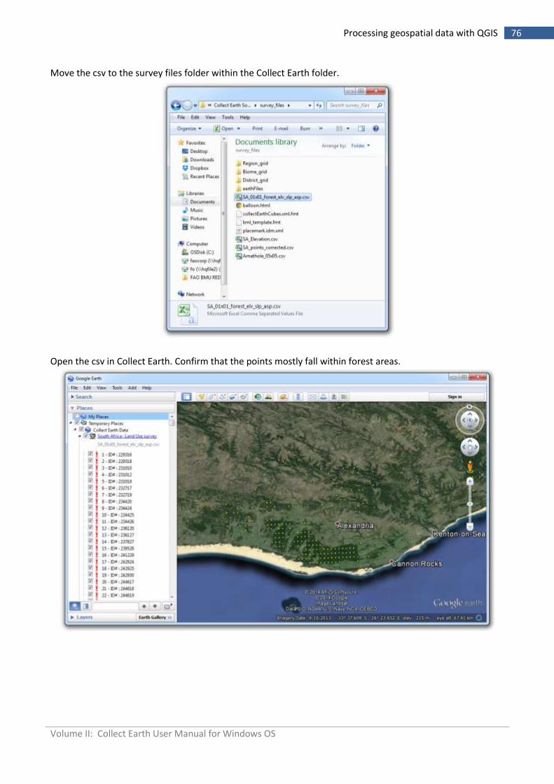
Move the csv to the survey files folder within the Collect Earth folder.
Open the csv in Collect Earth. Confirm that the points mostly fall within forest areas.
Volume II: Collect Earth User Manual for Windows OS
77 Processing geospatial data with QGIS
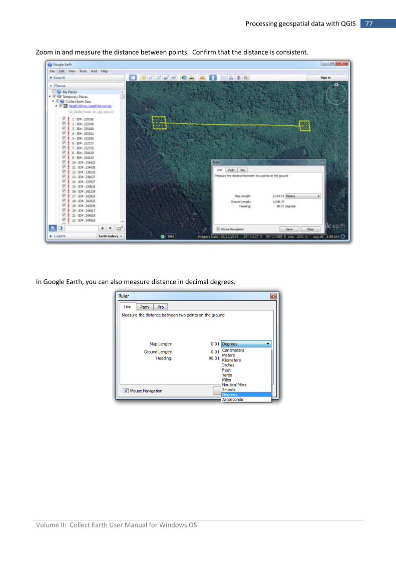
Zoom in and measure the distance between points. Confirm that the distance is consistent.
In Google Earth, you can also measure distance in decimal degrees.
Volume II: Collect Earth User Manual for Windows OS
78 Synergies between the Collect Earth sampling and Wall-to-Wall mapping
6 Synergies between the Collect Earth sampling and Wall-to-Wall mapping
6.1 Preparing vector data in Google Fusion Tables
6.1.1 Importing Collect Earth data into Google Fusion Tables
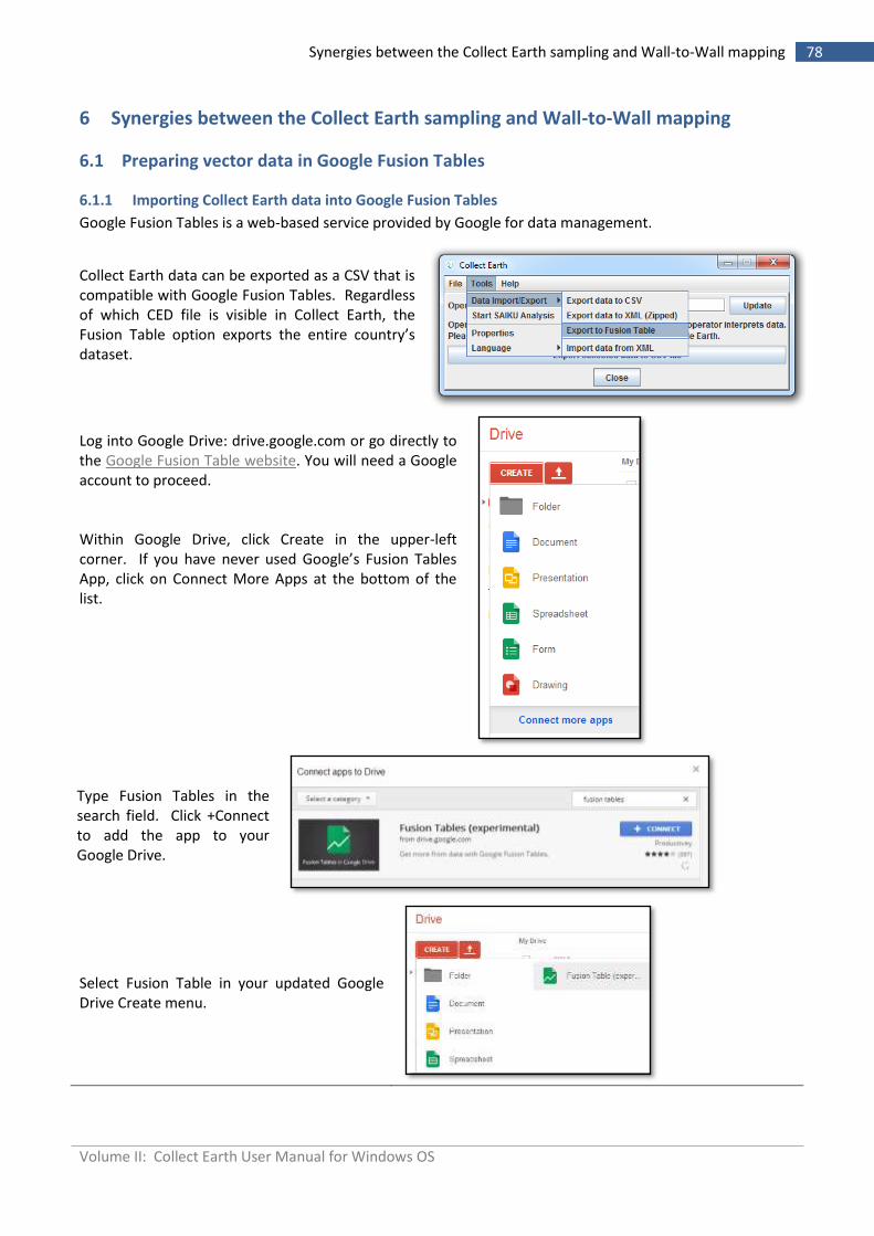
Google Fusion Tables is a web-based service provided by Google for data management.
Collect Earth data can be exported as a CSV that is compatible with Google Fusion Tables. Regardless of which CED file is visible in Collect Earth, the Fusion Table option exports the entire country’s dataset.
Log into Google Drive: drive.google.com or go directly to the Google Fusion Table website. You will need a Google account to proceed. Within Google Drive, click Create in the upper-left corner. If you have never used Google’s Fusion Tables App, click on Connect More Apps at the bottom of the list.
Type Fusion Tables in the search field. Click +Connect to add the app to your Google Drive.
Select Fusion Table in your updated Google Drive Create menu.
Volume II: Collect Earth User Manual for Windows OS
79 Synergies between the Collect Earth sampling and Wall-to-Wall mapping
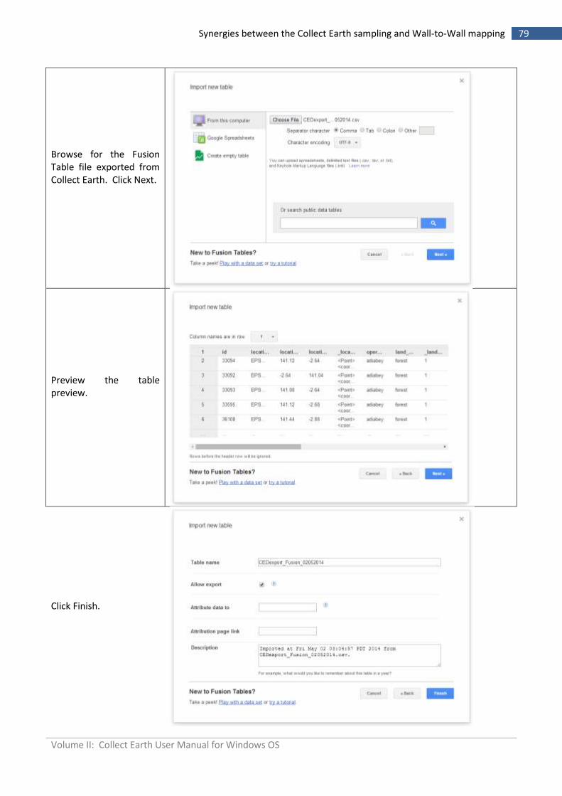
Browse for the Fusion Table file exported from Collect Earth. Click Next.
Preview the table preview.
Click Finish.
Volume II: Collect Earth User Manual for Windows OS
80 Synergies between the Collect Earth sampling and Wall-to-Wall mapping
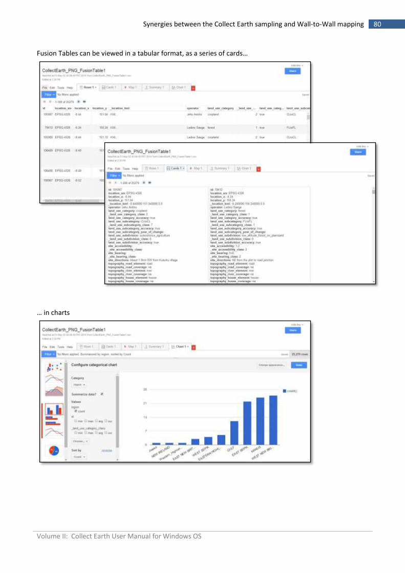
Fusion Tables can be viewed in a tabular format, as a series of cards…
… in charts
Volume II: Collect Earth User Manual for Windows OS
81 Synergies between the Collect Earth sampling and Wall-to-Wall mapping
… or in a map. This last option is useful for quickly reviewing spatial data that will be used in Earth Engine.
If Google Fusion Tables has difficultly geocoding the data, Earth Engine may not be able to display it. Collect
Earth facilitates data compatibility by concatenating the coordinates of each point into a single column, that
is identified as the location
column. Vector data from
other sources can also be
imported into Fusion Tables
(and later imported into Earth
Engine). If the data does not
properly geocode, the data
may be poorly positioned or a
message may appear
regarding the lack of a
location column.
To indicate which column contains the location data, return to the Rows tab, click on the header or the column that contains location data and select Change.
Click on the dropdown arrow under Type and select Location. Save changes.
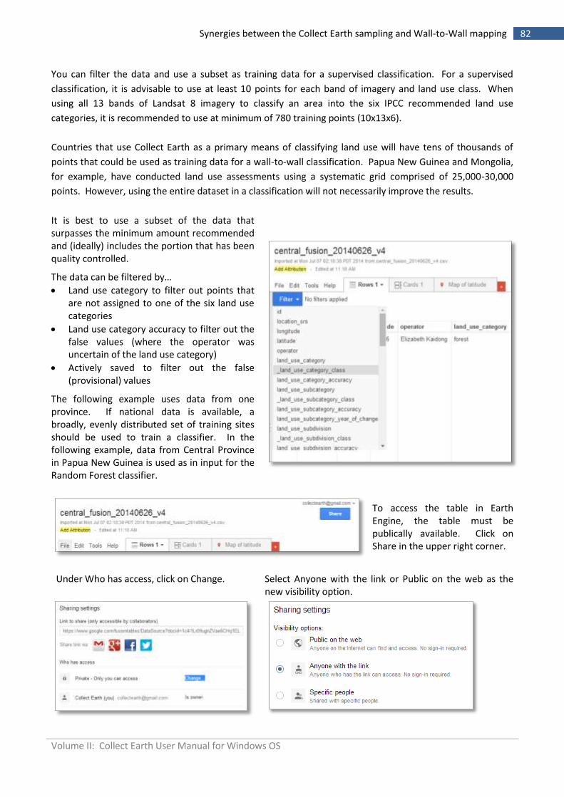
Volume II: Collect Earth User Manual for Windows OS
82 Synergies between the Collect Earth sampling and Wall-to-Wall mapping
You can filter the data and use a subset as training data for a supervised classification. For a supervised
classification, it is advisable to use at least 10 points for each band of imagery and land use class. When
using all 13 bands of Landsat 8 imagery to classify an area into the six IPCC recommended land use
categories, it is recommended to use at minimum of 780 training points (10x13x6).
Countries that use Collect Earth as a primary means of classifying land use will have tens of thousands of
points that could be used as training data for a wall-to-wall classification. Papua New Guinea and Mongolia,
for example, have conducted land use assessments using a systematic grid comprised of 25,000-30,000
points. However, using the entire dataset in a classification will not necessarily improve the results.
It is best to use a subset of the data that surpasses the minimum amount recommended and (ideally) includes the portion that has been quality controlled.
The data can be filtered by…
Land use category to filter out points that are not assigned to one of the six land use categories
Land use category accuracy to filter out the false values (where the operator was uncertain of the land use category)
Actively saved to filter out the false (provisional) values
The following example uses data from one province. If national data is available, a broadly, evenly distributed set of training sites should be used to train a classifier. In the following example, data from Central Province in Papua New Guinea is used as in input for the Random Forest classifier.
To access the table in Earth Engine, the table must be publically available. Click on Share in the upper right corner.
Under Who has access, click on Change.
Select Anyone with the link or Public on the web as the new visibility option.
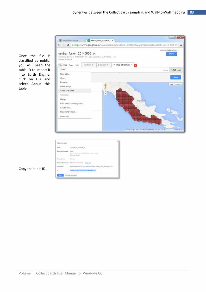
Volume II: Collect Earth User Manual for Windows OS
83 Synergies between the Collect Earth sampling and Wall-to-Wall mapping
Once the file is classified as public, you will need the table ID to import it into Earth Engine. Click on File and select About this table.
Copy the table ID.
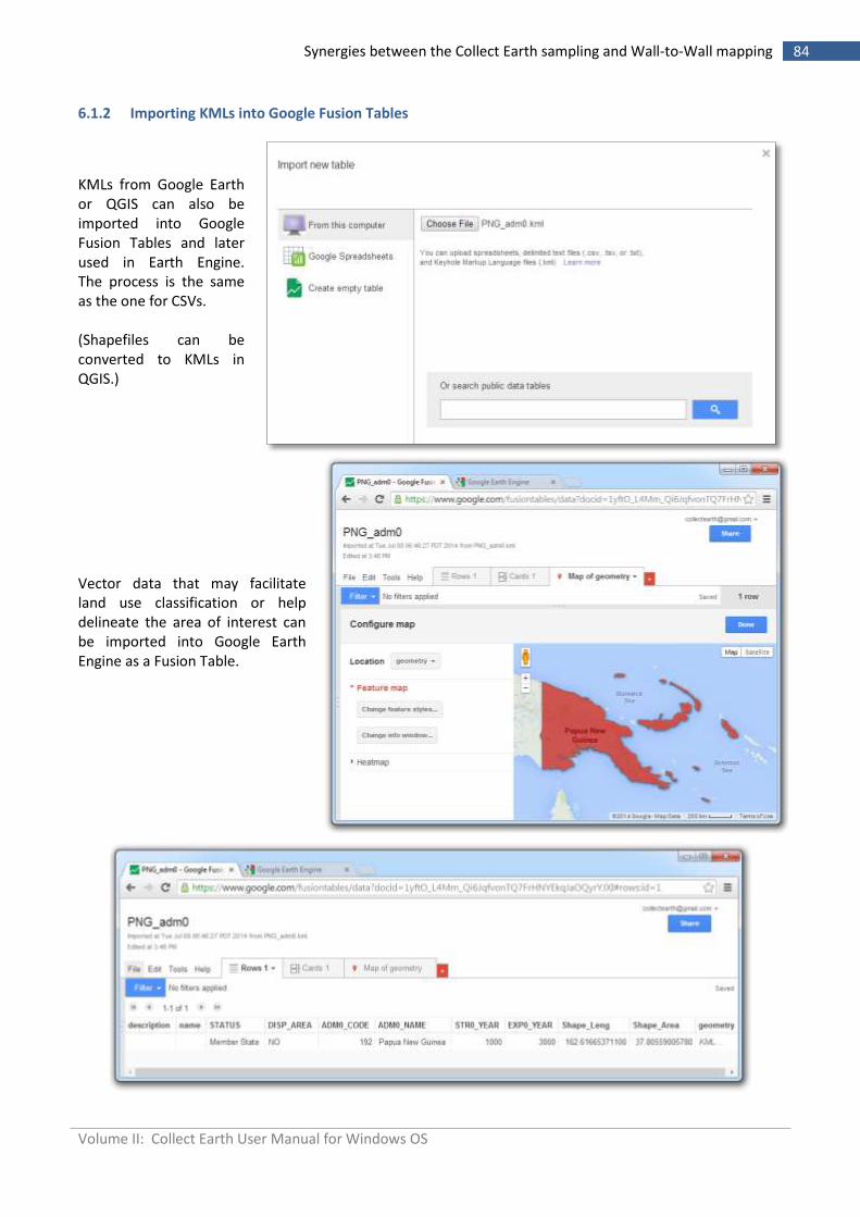
Volume II: Collect Earth User Manual for Windows OS
84 Synergies between the Collect Earth sampling and Wall-to-Wall mapping
6.1.2 Importing KMLs into Google Fusion Tables
KMLs from Google Earth or QGIS can also be imported into Google Fusion Tables and later used in Earth Engine. The process is the same as the one for CSVs. (Shapefiles can be converted to KMLs in QGIS.)
Vector data that may facilitate land use classification or help delineate the area of interest can be imported into Google Earth Engine as a Fusion Table.
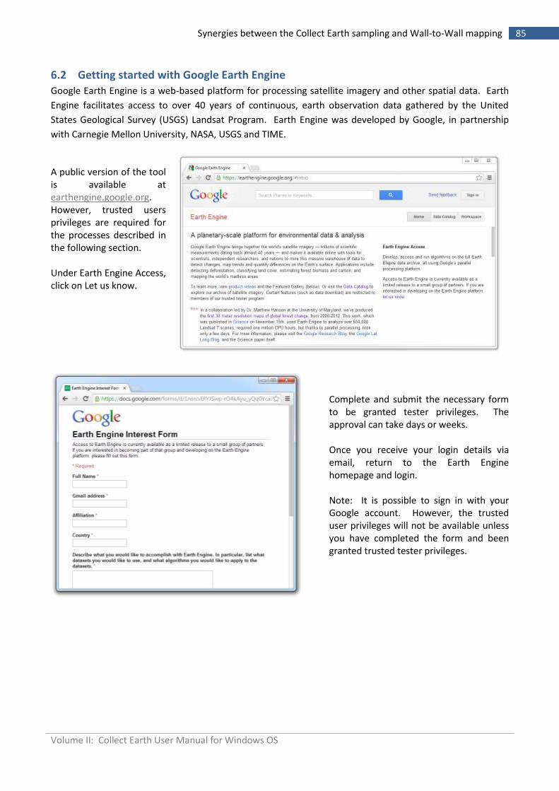
Volume II: Collect Earth User Manual for Windows OS
85 Synergies between the Collect Earth sampling and Wall-to-Wall mapping
6.2 Getting started with Google Earth Engine
Google Earth Engine is a web-based platform for processing satellite imagery and other spatial data. Earth
Engine facilitates access to over 40 years of continuous, earth observation data gathered by the United
States Geological Survey (USGS) Landsat Program. Earth Engine was developed by Google, in partnership
with Carnegie Mellon University, NASA, USGS and TIME.
A public version of the tool is available at earthengine.google.org. However, trusted users privileges are required for the processes described in the following section. Under Earth Engine Access, click on Let us know.
Complete and submit the necessary form to be granted tester privileges. The approval can take days or weeks. Once you receive your login details via email, return to the Earth Engine homepage and login. Note: It is possible to sign in with your Google account. However, the trusted user privileges will not be available unless you have completed the form and been granted trusted tester privileges.
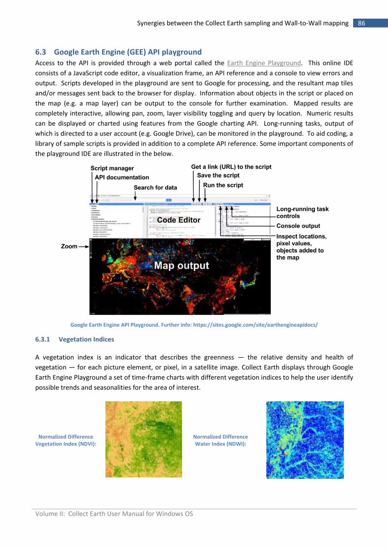
Volume II: Collect Earth User Manual for Windows OS
86 Synergies between the Collect Earth sampling and Wall-to-Wall mapping
6.3 Google Earth Engine (GEE) API playground
Access to the API is provided through a web portal called the Earth Engine Playground. This online IDE
consists of a JavaScript code editor, a visualization frame, an API reference and a console to view errors and
output. Scripts developed in the playground are sent to Google for processing, and the resultant map tiles
and/or messages sent back to the browser for display. Information about objects in the script or placed on
the map (e.g. a map layer) can be output to the console for further examination. Mapped results are
completely interactive, allowing pan, zoom, layer visibility toggling and query by location. Numeric results
can be displayed or charted using features from the Google charting API. Long-running tasks, output of
which is directed to a user account (e.g. Google Drive), can be monitored in the playground. To aid coding, a
library of sample scripts is provided in addition to a complete API reference. Some important components of
the playground IDE are illustrated in the below.
Google Earth Engine API Playground. Further info: https://sites.google.com/site/earthengineapidocs/
6.3.1 Vegetation Indices
A vegetation index is an indicator that describes the greenness — the relative density and health of
vegetation — for each picture element, or pixel, in a satellite image. Collect Earth displays through Google
Earth Engine Playground a set of time-frame charts with different vegetation indices to help the user identify
possible trends and seasonalities for the area of interest.
Normalized Difference Vegetation Index (NDVI):
Normalized Difference Water Index (NDWI):
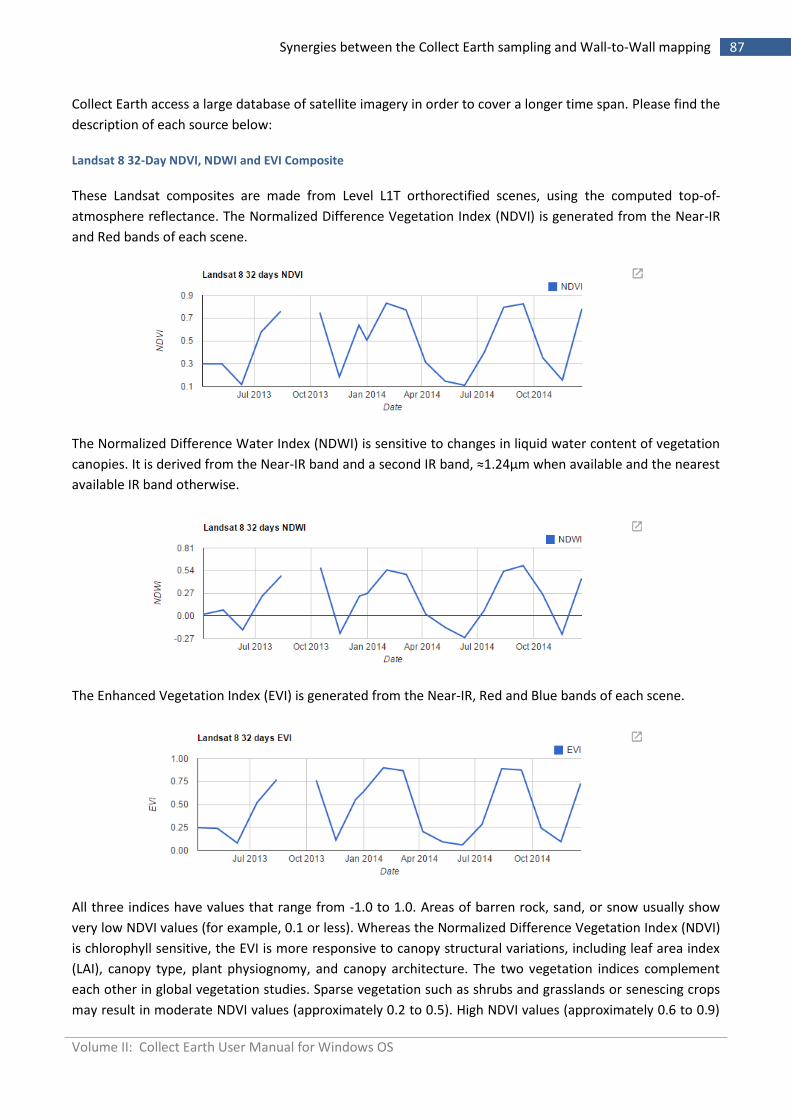
Volume II: Collect Earth User Manual for Windows OS
87 Synergies between the Collect Earth sampling and Wall-to-Wall mapping
Collect Earth access a large database of satellite imagery in order to cover a longer time span. Please find the
description of each source below:
Landsat 8 32-Day NDVI, NDWI and EVI Composite
These Landsat composites are made from Level L1T orthorectified scenes, using the computed top-of-
atmosphere reflectance. The Normalized Difference Vegetation Index (NDVI) is generated from the Near-IR
and Red bands of each scene.
The Normalized Difference Water Index (NDWI) is sensitive to changes in liquid water content of vegetation
canopies. It is derived from the Near-IR band and a second IR band, ≈1.24μm when available and the nearest
available IR band otherwise.
The Enhanced Vegetation Index (EVI) is generated from the Near-IR, Red and Blue bands of each scene.
All three indices have values that range from -1.0 to 1.0. Areas of barren rock, sand, or snow usually show
very low NDVI values (for example, 0.1 or less). Whereas the Normalized Difference Vegetation Index (NDVI)
is chlorophyll sensitive, the EVI is more responsive to canopy structural variations, including leaf area index
(LAI), canopy type, plant physiognomy, and canopy architecture. The two vegetation indices complement
each other in global vegetation studies. Sparse vegetation such as shrubs and grasslands or senescing crops
may result in moderate NDVI values (approximately 0.2 to 0.5). High NDVI values (approximately 0.6 to 0.9)
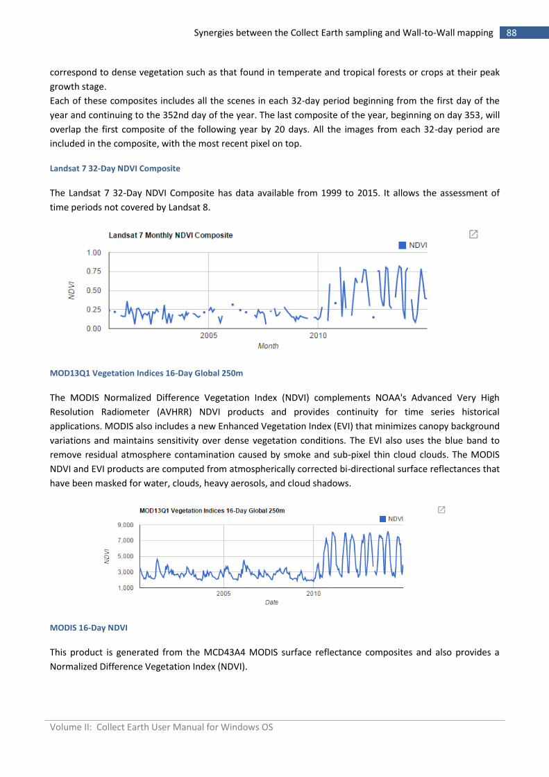
Volume II: Collect Earth User Manual for Windows OS
88 Synergies between the Collect Earth sampling and Wall-to-Wall mapping
correspond to dense vegetation such as that found in temperate and tropical forests or crops at their peak
growth stage.
Each of these composites includes all the scenes in each 32-day period beginning from the first day of the
year and continuing to the 352nd day of the year. The last composite of the year, beginning on day 353, will
overlap the first composite of the following year by 20 days. All the images from each 32-day period are
included in the composite, with the most recent pixel on top.
Landsat 7 32-Day NDVI Composite
The Landsat 7 32-Day NDVI Composite has data available from 1999 to 2015. It allows the assessment of
time periods not covered by Landsat 8.
MOD13Q1 Vegetation Indices 16-Day Global 250m
The MODIS Normalized Difference Vegetation Index (NDVI) complements NOAA's Advanced Very High
Resolution Radiometer (AVHRR) NDVI products and provides continuity for time series historical
applications. MODIS also includes a new Enhanced Vegetation Index (EVI) that minimizes canopy background
variations and maintains sensitivity over dense vegetation conditions. The EVI also uses the blue band to
remove residual atmosphere contamination caused by smoke and sub-pixel thin cloud clouds. The MODIS
NDVI and EVI products are computed from atmospherically corrected bi-directional surface reflectances that
have been masked for water, clouds, heavy aerosols, and cloud shadows.
MODIS 16-Day NDVI
This product is generated from the MCD43A4 MODIS surface reflectance composites and also provides a
Normalized Difference Vegetation Index (NDVI).
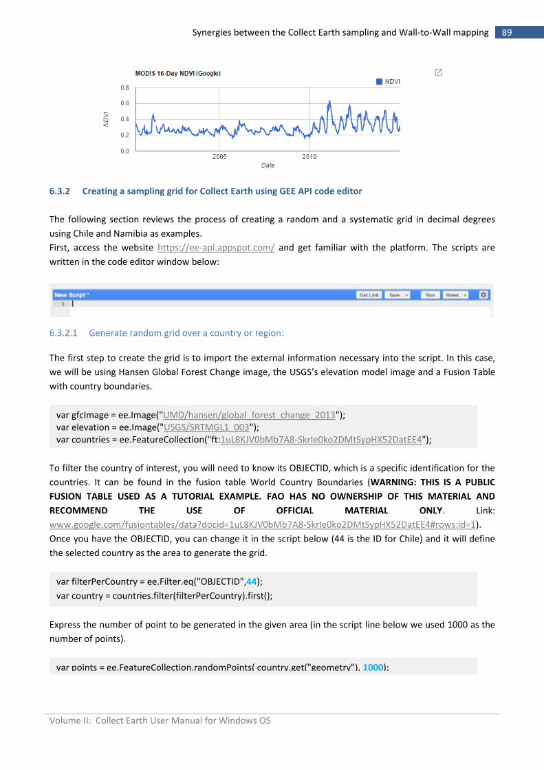
Volume II: Collect Earth User Manual for Windows OS
89 Synergies between the Collect Earth sampling and Wall-to-Wall mapping
6.3.2 Creating a sampling grid for Collect Earth using GEE API code editor
The following section reviews the process of creating a random and a systematic grid in decimal degrees
using Chile and Namibia as examples.
First, access the website https://ee-api.appspot.com/ and get familiar with the platform. The scripts are
written in the code editor window below:
6.3.2.1 Generate random grid over a country or region:
The first step to create the grid is to import the external information necessary into the script. In this case,
we will be using Hansen Global Forest Change image, the USGS’s elevation model image and a Fusion Table
with country boundaries.
To filter the country of interest, you will need to know its OBJECTID, which is a specific identification for the
countries. It can be found in the fusion table World Country Boundaries (WARNING: THIS IS A PUBLIC
FUSION TABLE USED AS A TUTORIAL EXAMPLE. FAO HAS NO OWNERSHIP OF THIS MATERIAL AND
RECOMMEND THE USE OF OFFICIAL MATERIAL ONLY. Link:
www.google.com/fusiontables/data?docid=1uL8KJV0bMb7A8-SkrIe0ko2DMtSypHX52DatEE4#rows:id=1).
Once you have the OBJECTID, you can change it in the script below (44 is the ID for Chile) and it will define
the selected country as the area to generate the grid.
Express the number of point to be generated in the given area (in the script line below we used 1000 as the
number of points).
var gfcImage = ee.Image("UMD/hansen/global_forest_change_2013"); var elevation = ee.Image("USGS/SRTMGL1_003"); var countries = ee.FeatureCollection("ft:1uL8KJV0bMb7A8-SkrIe0ko2DMtSypHX52DatEE4");
var filterPerCountry = ee.Filter.eq("OBJECTID",44);
var country = countries.filter(filterPerCountry).first();
var points = ee.FeatureCollection.randomPoints( country.get("geometry"), 1000);
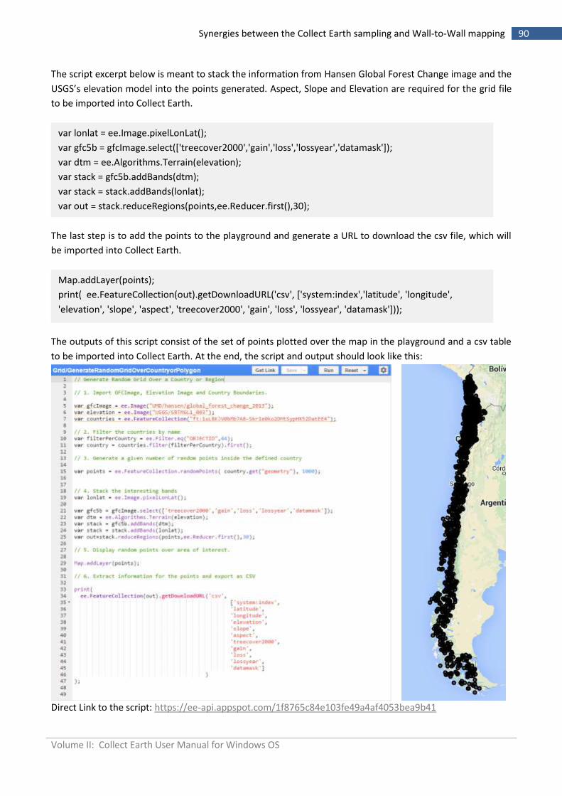
Volume II: Collect Earth User Manual for Windows OS
90 Synergies between the Collect Earth sampling and Wall-to-Wall mapping
The script excerpt below is meant to stack the information from Hansen Global Forest Change image and the
USGS’s elevation model into the points generated. Aspect, Slope and Elevation are required for the grid file
to be imported into Collect Earth.
The last step is to add the points to the playground and generate a URL to download the csv file, which will
be imported into Collect Earth.
The outputs of this script consist of the set of points plotted over the map in the playground and a csv table
to be imported into Collect Earth. At the end, the script and output should look like this:
Direct Link to the script: https://ee-api.appspot.com/1f8765c84e103fe49a4af4053bea9b41
var lonlat = ee.Image.pixelLonLat();
var gfc5b = gfcImage.select(['treecover2000','gain','loss','lossyear','datamask']);
var dtm = ee.Algorithms.Terrain(elevation);
var stack = gfc5b.addBands(dtm);
var stack = stack.addBands(lonlat);
var out = stack.reduceRegions(points,ee.Reducer.first(),30);
Map.addLayer(points);
print( ee.FeatureCollection(out).getDownloadURL('csv', ['system:index','latitude', 'longitude',
'elevation', 'slope', 'aspect', 'treecover2000', 'gain', 'loss', 'lossyear', 'datamask']));
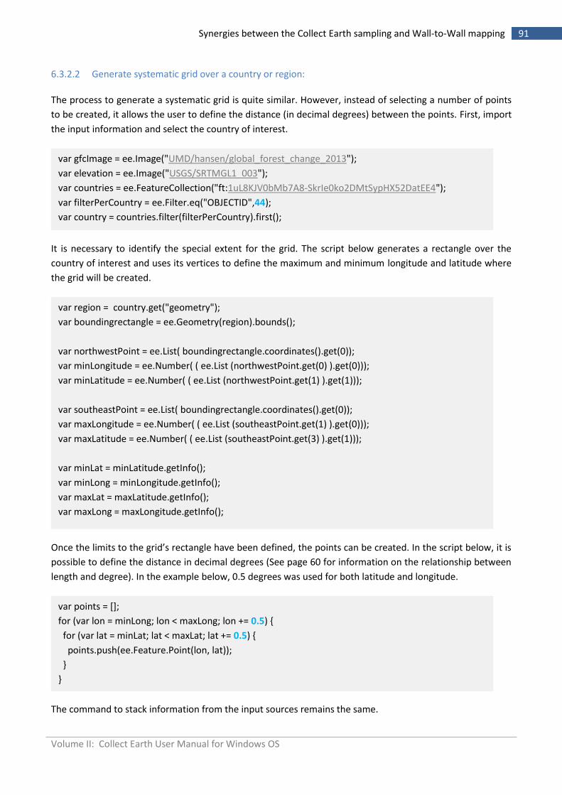
Volume II: Collect Earth User Manual for Windows OS
91 Synergies between the Collect Earth sampling and Wall-to-Wall mapping
6.3.2.2 Generate systematic grid over a country or region:
The process to generate a systematic grid is quite similar. However, instead of selecting a number of points
to be created, it allows the user to define the distance (in decimal degrees) between the points. First, import
the input information and select the country of interest.
It is necessary to identify the special extent for the grid. The script below generates a rectangle over the
country of interest and uses its vertices to define the maximum and minimum longitude and latitude where
the grid will be created.
Once the limits to the grid’s rectangle have been defined, the points can be created. In the script below, it is
possible to define the distance in decimal degrees (See page 60 for information on the relationship between
length and degree). In the example below, 0.5 degrees was used for both latitude and longitude.
The command to stack information from the input sources remains the same.
var gfcImage = ee.Image("UMD/hansen/global_forest_change_2013");
var elevation = ee.Image("USGS/SRTMGL1_003");
var countries = ee.FeatureCollection("ft:1uL8KJV0bMb7A8-SkrIe0ko2DMtSypHX52DatEE4");
var filterPerCountry = ee.Filter.eq("OBJECTID",44);
var country = countries.filter(filterPerCountry).first();
var region = country.get("geometry");
var boundingrectangle = ee.Geometry(region).bounds();
var northwestPoint = ee.List( boundingrectangle.coordinates().get(0));
var minLongitude = ee.Number( ( ee.List (northwestPoint.get(0) ).get(0)));
var minLatitude = ee.Number( ( ee.List (northwestPoint.get(1) ).get(1)));
var southeastPoint = ee.List( boundingrectangle.coordinates().get(0));
var maxLongitude = ee.Number( ( ee.List (southeastPoint.get(1) ).get(0)));
var maxLatitude = ee.Number( ( ee.List (southeastPoint.get(3) ).get(1)));
var minLat = minLatitude.getInfo();
var minLong = minLongitude.getInfo();
var maxLat = maxLatitude.getInfo();
var maxLong = maxLongitude.getInfo();
var points = [];
for (var lon = minLong; lon < maxLong; lon += 0.5) {
for (var lat = minLat; lat < maxLat; lat += 0.5) {
points.push(ee.Feature.Point(lon, lat));
}
}
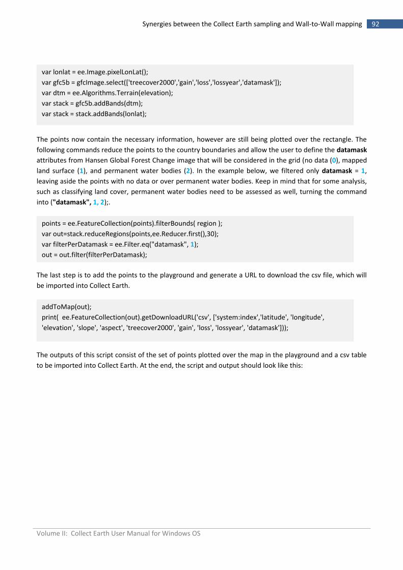
Volume II: Collect Earth User Manual for Windows OS
92 Synergies between the Collect Earth sampling and Wall-to-Wall mapping
The points now contain the necessary information, however are still being plotted over the rectangle. The
following commands reduce the points to the country boundaries and allow the user to define the datamask
attributes from Hansen Global Forest Change image that will be considered in the grid (no data (0), mapped
land surface (1), and permanent water bodies (2). In the example below, we filtered only datamask = 1,
leaving aside the points with no data or over permanent water bodies. Keep in mind that for some analysis,
such as classifying land cover, permanent water bodies need to be assessed as well, turning the command
into ("datamask", 1, 2);.
The last step is to add the points to the playground and generate a URL to download the csv file, which will
be imported into Collect Earth.
The outputs of this script consist of the set of points plotted over the map in the playground and a csv table
to be imported into Collect Earth. At the end, the script and output should look like this:
var lonlat = ee.Image.pixelLonLat();
var gfc5b = gfcImage.select(['treecover2000','gain','loss','lossyear','datamask']);
var dtm = ee.Algorithms.Terrain(elevation);
var stack = gfc5b.addBands(dtm);
var stack = stack.addBands(lonlat);
points = ee.FeatureCollection(points).filterBounds( region );
var out=stack.reduceRegions(points,ee.Reducer.first(),30);
var filterPerDatamask = ee.Filter.eq("datamask", 1);
out = out.filter(filterPerDatamask);
addToMap(out);
print( ee.FeatureCollection(out).getDownloadURL('csv', ['system:index','latitude', 'longitude',
'elevation', 'slope', 'aspect', 'treecover2000', 'gain', 'loss', 'lossyear', 'datamask']));
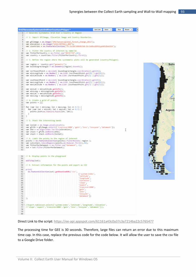
Volume II: Collect Earth User Manual for Windows OS
93 Synergies between the Collect Earth sampling and Wall-to-Wall mapping
Direct Link to the script: https://ee-api.appspot.com/61161a43c0a37c3a7214ba22c5765477
The processing time for GEE is 30 seconds. Therefore, large files can return an error due to this maximum
time cap. In this case, replace the previous code for the code below. It will allow the user to save the csv file
to a Google Drive folder.
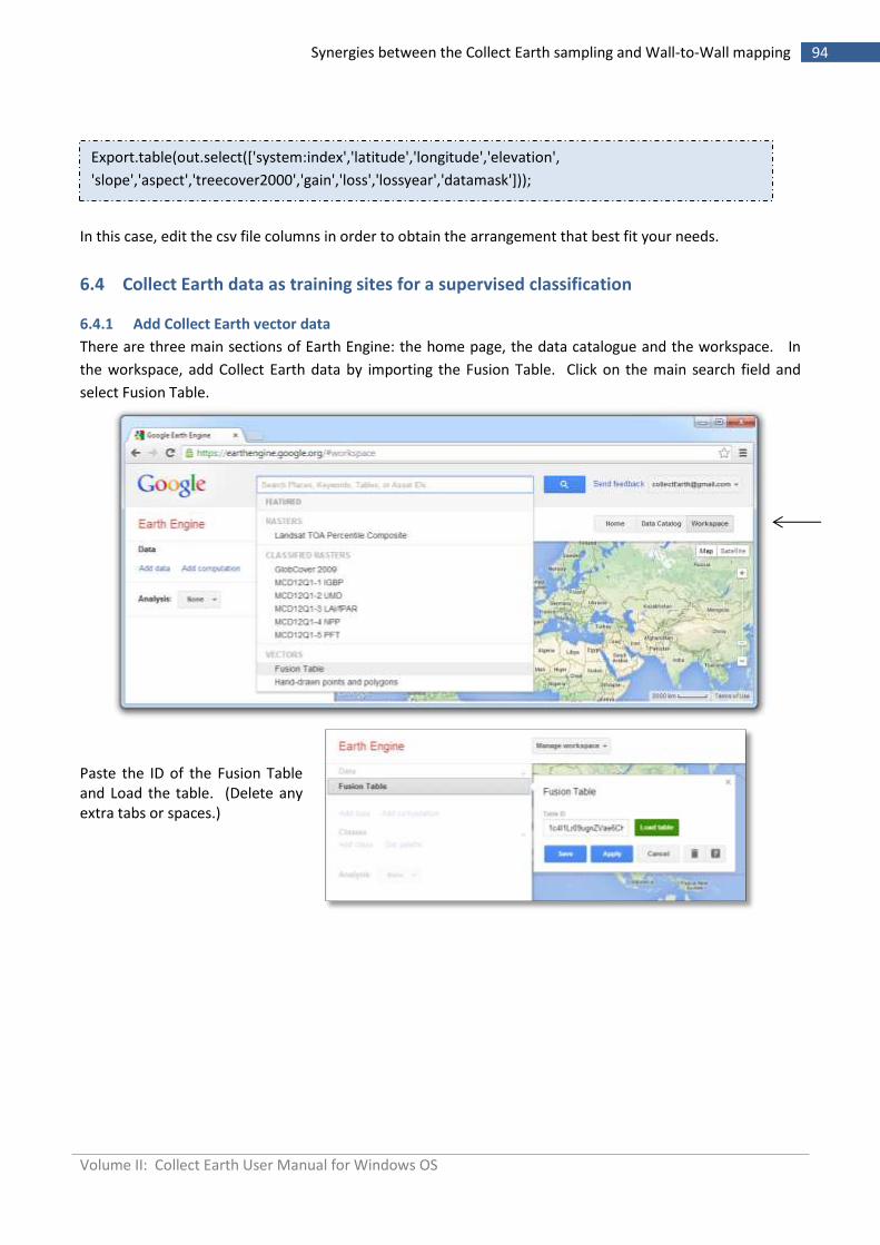
Volume II: Collect Earth User Manual for Windows OS
94 Synergies between the Collect Earth sampling and Wall-to-Wall mapping
In this case, edit the csv file columns in order to obtain the arrangement that best fit your needs.
6.4 Collect Earth data as training sites for a supervised classification
6.4.1 Add Collect Earth vector data
There are three main sections of Earth Engine: the home page, the data catalogue and the workspace. In
the workspace, add Collect Earth data by importing the Fusion Table. Click on the main search field and
select Fusion Table.
Paste the ID of the Fusion Table and Load the table. (Delete any extra tabs or spaces.)
Export.table(out.select(['system:index','latitude','longitude','elevation',
'slope','aspect','treecover2000','gain','loss','lossyear','datamask']));
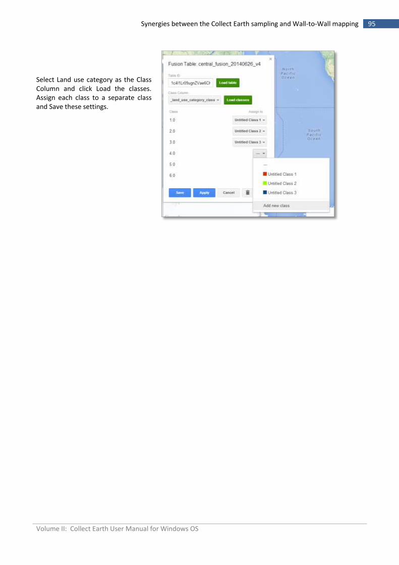
Volume II: Collect Earth User Manual for Windows OS
95 Synergies between the Collect Earth sampling and Wall-to-Wall mapping
Select Land use category as the Class Column and click Load the classes. Assign each class to a separate class and Save these settings.
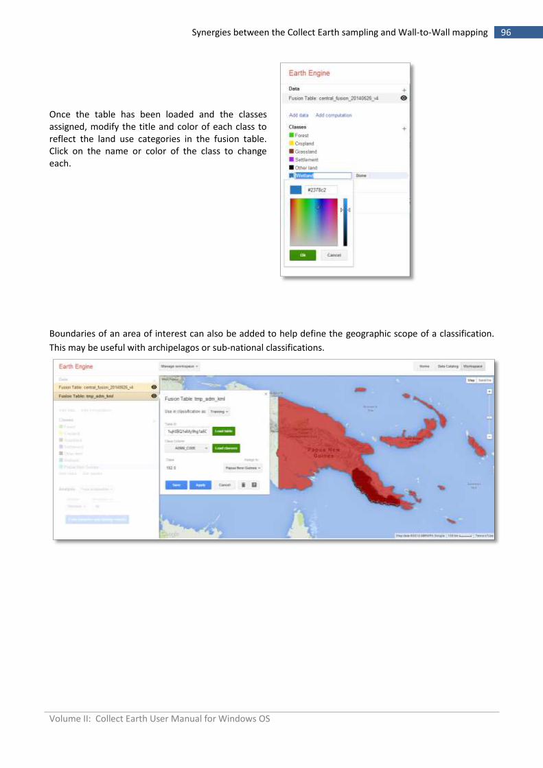
Volume II: Collect Earth User Manual for Windows OS
96 Synergies between the Collect Earth sampling and Wall-to-Wall mapping
Boundaries of an area of interest can also be added to help define the geographic scope of a classification.
This may be useful with archipelagos or sub-national classifications.
Once the table has been loaded and the classes assigned, modify the title and color of each class to reflect the land use categories in the fusion table. Click on the name or color of the class to change each.
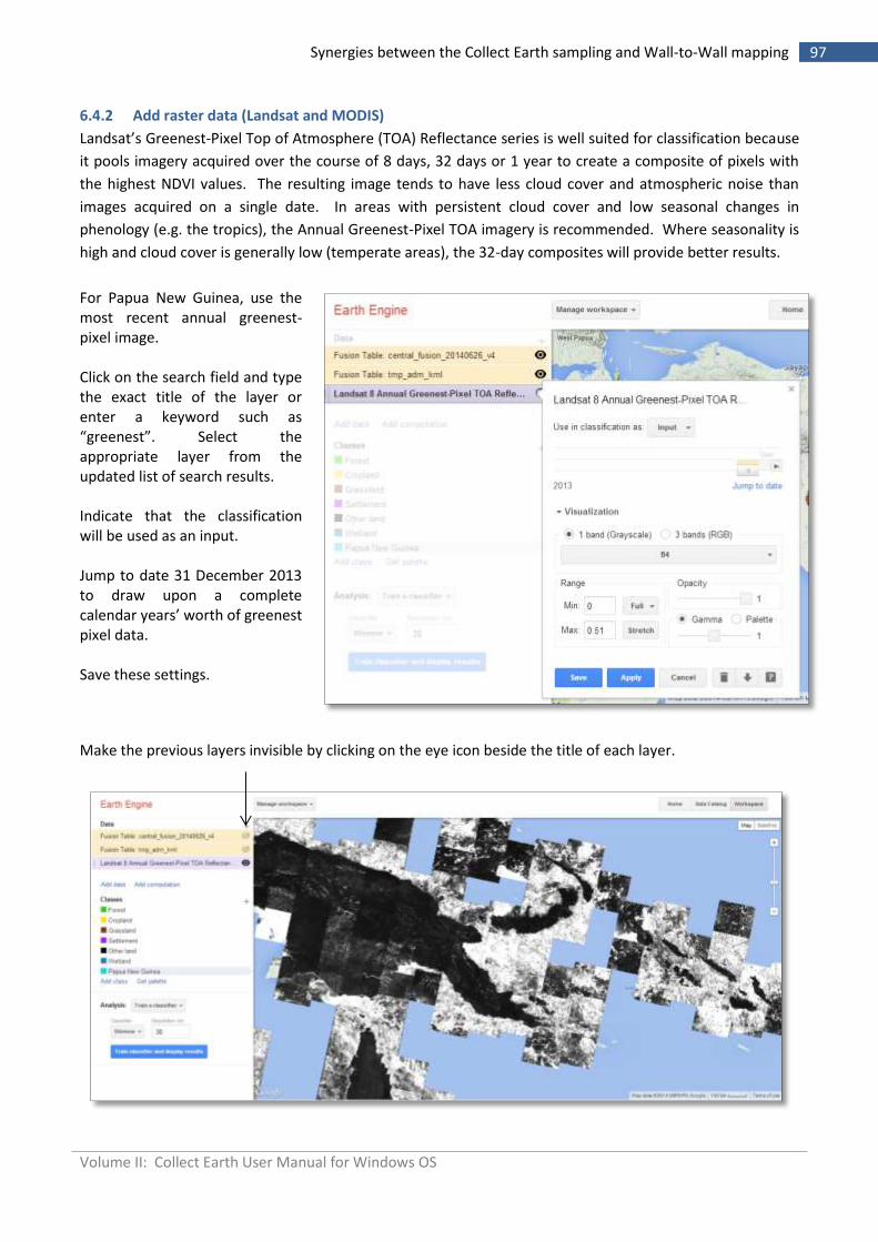
Volume II: Collect Earth User Manual for Windows OS
97 Synergies between the Collect Earth sampling and Wall-to-Wall mapping
6.4.2 Add raster data (Landsat and MODIS)
Landsat’s Greenest-Pixel Top of Atmosphere (TOA) Reflectance series is well suited for classification because
it pools imagery acquired over the course of 8 days, 32 days or 1 year to create a composite of pixels with
the highest NDVI values. The resulting image tends to have less cloud cover and atmospheric noise than
images acquired on a single date. In areas with persistent cloud cover and low seasonal changes in
phenology (e.g. the tropics), the Annual Greenest-Pixel TOA imagery is recommended. Where seasonality is
high and cloud cover is generally low (temperate areas), the 32-day composites will provide better results.
For Papua New Guinea, use the most recent annual greenest-pixel image. Click on the search field and type the exact title of the layer or enter a keyword such as “greenest”. Select the appropriate layer from the updated list of search results. Indicate that the classification will be used as an input. Jump to date 31 December 2013 to draw upon a complete calendar years’ worth of greenest pixel data. Save these settings.
Make the previous layers invisible by clicking on the eye icon beside the title of each layer.
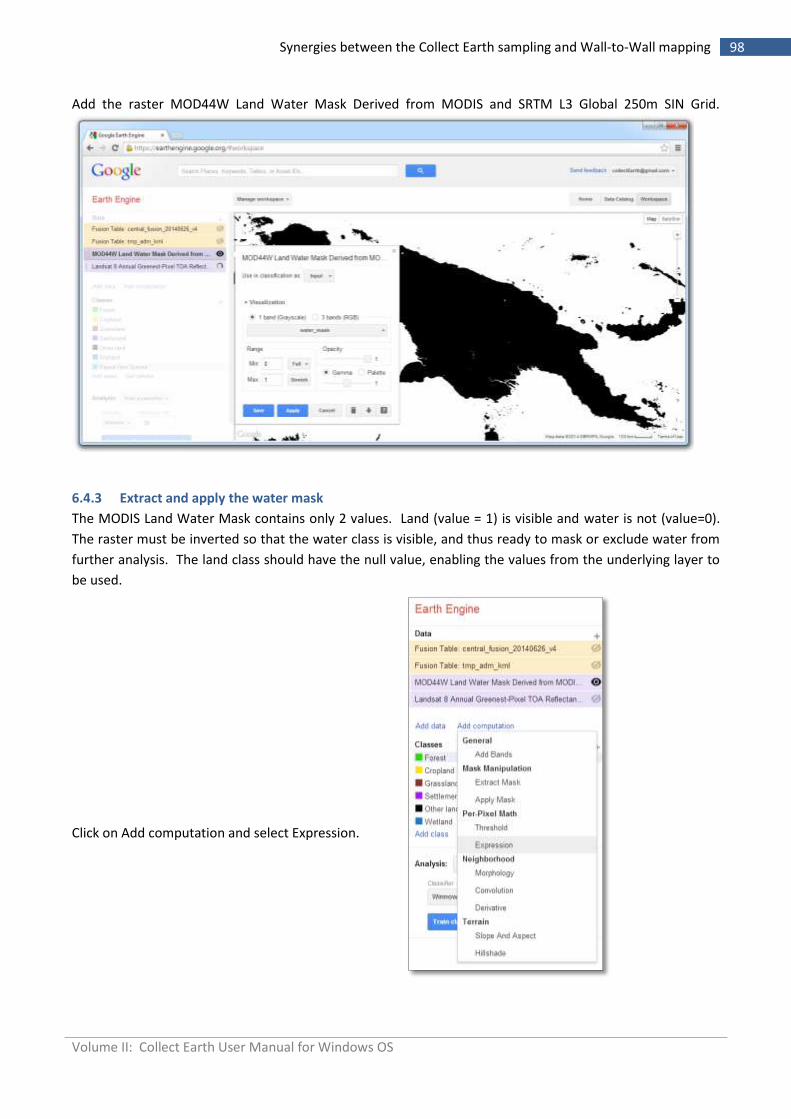
Volume II: Collect Earth User Manual for Windows OS
98 Synergies between the Collect Earth sampling and Wall-to-Wall mapping
Add the raster MOD44W Land Water Mask Derived from MODIS and SRTM L3 Global 250m SIN Grid.
6.4.3 Extract and apply the water mask
The MODIS Land Water Mask contains only 2 values. Land (value = 1) is visible and water is not (value=0).
The raster must be inverted so that the water class is visible, and thus ready to mask or exclude water from
further analysis. The land class should have the null value, enabling the values from the underlying layer to
be used.
Click on Add computation and select Expression.
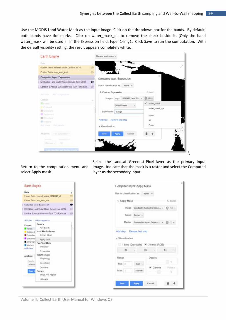
Volume II: Collect Earth User Manual for Windows OS
99 Synergies between the Collect Earth sampling and Wall-to-Wall mapping
Use the MODIS Land Water Mask as the input image. Click on the dropdown box for the bands. By default,
both bands have tics marks. Click on water_mask_qa to remove the check beside it. (Only the band
water_mask will be used.) In the Expression field, type: 1-img1. Click Save to run the computation. With
the default visibility setting, the result appears completely white.
\
Return to the computation menu and select Apply mask.
Select the Landsat Greenest-Pixel layer as the primary input image. Indicate that the mask is a raster and select the Computed layer as the secondary input.
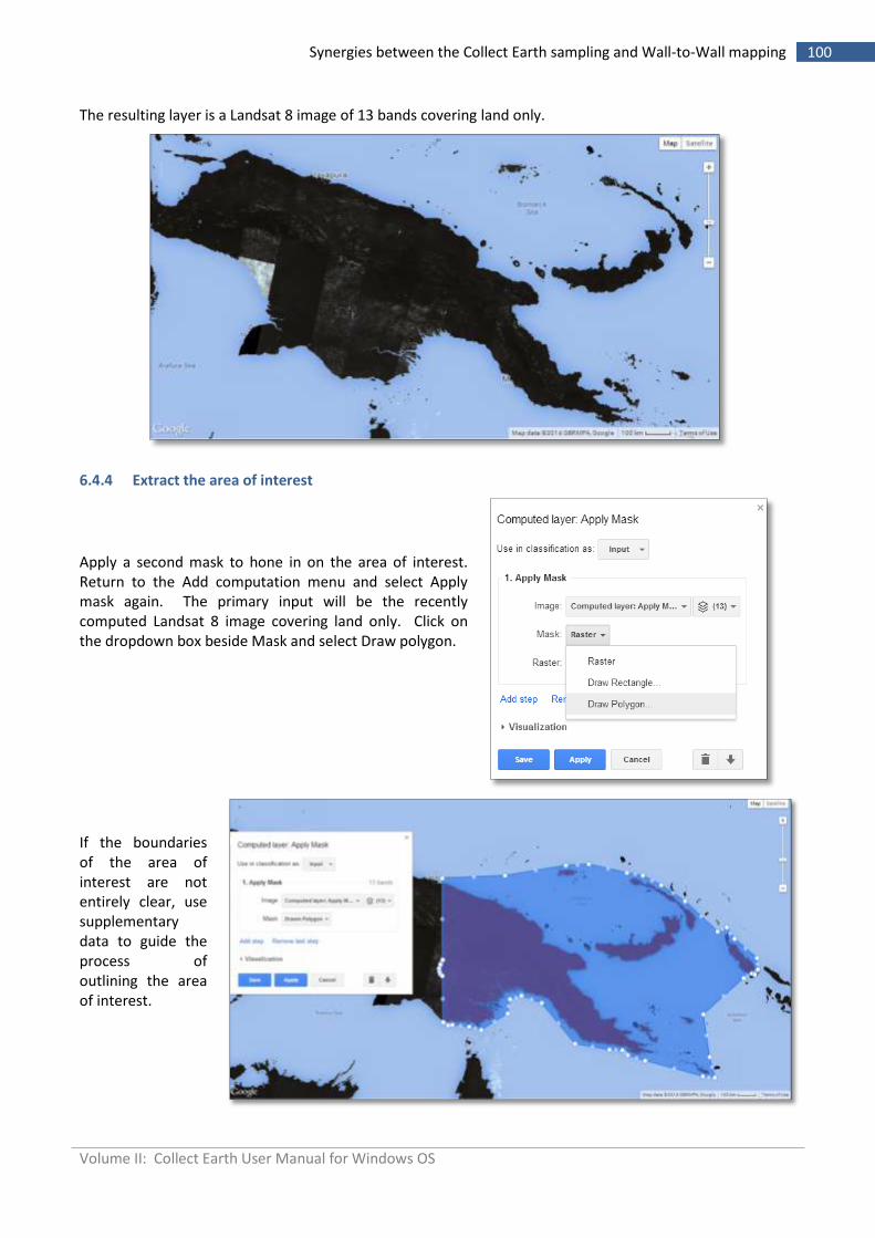
Volume II: Collect Earth User Manual for Windows OS
100 Synergies between the Collect Earth sampling and Wall-to-Wall mapping
The resulting layer is a Landsat 8 image of 13 bands covering land only.
6.4.4 Extract the area of interest
Apply a second mask to hone in on the area of interest. Return to the Add computation menu and select Apply mask again. The primary input will be the recently computed Landsat 8 image covering land only. Click on the dropdown box beside Mask and select Draw polygon.
If the boundaries of the area of interest are not entirely clear, use supplementary data to guide the process of outlining the area of interest.
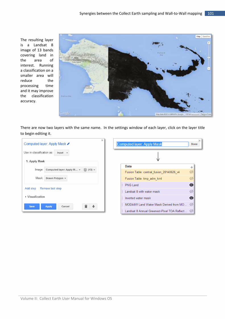
Volume II: Collect Earth User Manual for Windows OS
101 Synergies between the Collect Earth sampling and Wall-to-Wall mapping
The resulting layer is a Landsat 8 image of 13 bands covering land in the area of interest. Running a classification on a smaller area will reduce the processing time and it may improve the classification accuracy.
There are now two layers with the same name. In the settings window of each layer, click on the layer title
to begin editing it.
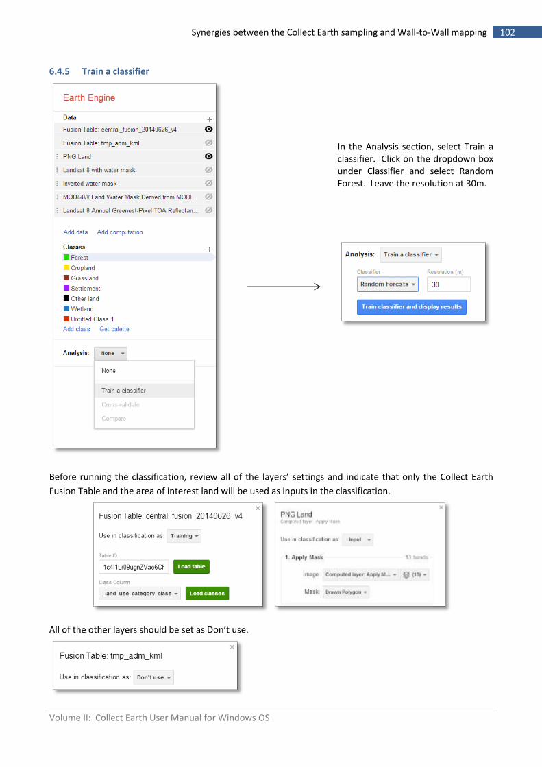
Volume II: Collect Earth User Manual for Windows OS
102 Synergies between the Collect Earth sampling and Wall-to-Wall mapping
6.4.5 Train a classifier
In the Analysis section, select Train a classifier. Click on the dropdown box under Classifier and select Random Forest. Leave the resolution at 30m.
Before running the classification, review all of the layers’ settings and indicate that only the Collect Earth
Fusion Table and the area of interest land will be used as inputs in the classification.
All of the other layers should be set as Don’t use.
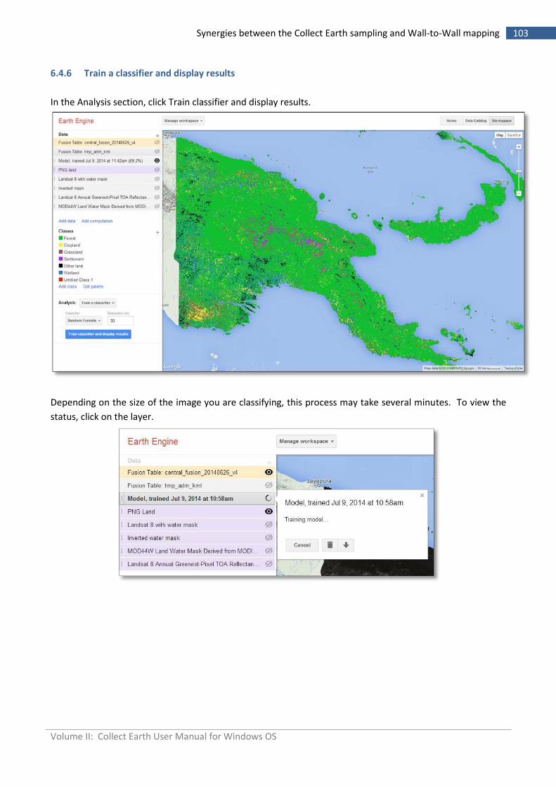
Volume II: Collect Earth User Manual for Windows OS
103 Synergies between the Collect Earth sampling and Wall-to-Wall mapping
6.4.6 Train a classifier and display results
In the Analysis section, click Train classifier and display results.
Depending on the size of the image you are classifying, this process may take several minutes. To view the
status, click on the layer.
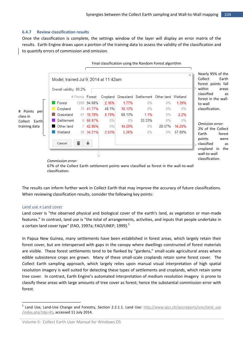
Volume II: Collect Earth User Manual for Windows OS
104 Synergies between the Collect Earth sampling and Wall-to-Wall mapping
6.4.7 Review classification results
Once the classification is complete, the settings window of the layer will display an error matrix of the
results. Earth Engine draws upon a portion of the training data to assess the validity of the classification and
to quantify errors of commission and omission.
Final classification using the Random Forest algorithm
# Points per class in Collect Earth training data
Commission error: 67% of the Collect Earth settlement points were classified as forest in the wall-to-wall classification.
Nearly 95% of the Collect Earth forest points fall within areas classified as forest in the wall-to-wall classification. Omission error: 2% of the Collect Earth forest points were classified as cropland in the wall-to-wall classification.
The results can inform further work in Collect Earth that may improve the accuracy of future classifications.
When reviewing classification results, consider the following key points:
Land use ≠ Land cover
Land cover is "the observed physical and biological cover of the earth's land, as vegetation or man-made
features." In contrast, land use is "the total of arrangements, activities, and inputs that people undertake in
a certain land cover type" (FAO, 1997a; FAO/UNEP, 1999).5
In Papua New Guinea, many settlements have been established in forest areas, which largely retain their
forest cover, but are interspersed with gaps in the canopy where dwellings constructed of forest materials
are visible. These forest settlements tend to be flanked by “gardens,” small-scale agricultural areas where
edible subsistence crops are grown. Many of these small-scale croplands retain some forest cover. The
Collect Earth sampling approach, which largely relies upon manual visual interpretation of high spatial
resolution imagery is well suited for detecting these types of settlements and croplands, which retain some
tree cover. In contrast, Earth Engine’s automated interpretation of medium resolution imagery is prone to
classify these areas with large amounts of tree cover as forest; hence the substantial commission error with
forest.
5 Land Use, Land-Use Change and Forestry, Section 2.2.1.1. Land Use: http://www.ipcc.ch/ipccreports/sres/land_use
/index.php?idp=45, accessed 11 July 2014.
Volume II: Collect Earth User Manual for Windows OS
105 Synergies between the Collect Earth sampling and Wall-to-Wall mapping
Classification objective
The validity of the classification is nearly 90%. While this figure is important, the validity of a particular class
may be of greater importance depending upon how the wall-to-wall classification will be used. If this
classification were intended to determine the spatial extent of forest and potential forest inventory sites,
this classification with 95% validity in the forest class might be suitable. However, a map with less than 50%
classification validity for the cropland, settlement and other land and would be inadequate for national
reporting of land use, land use change and forestry to the UNFCCC. This is particularly problematic because
such high levels of commission error with forest land is likely to inflate carbon stock values.
Stratified sampling and adequate sampling sizes
Drawing upon over one thousand training points, the Random Forest algorithm performs extremely well
when classifying forest areas. The remaining classes have 93% - 99.6% fewer training points, and
consequently, poorly defined class boundaries Increasing the number of training points for these under
represented classes through a stratified-random sampling scheme may improve the overall validity of the
classification.
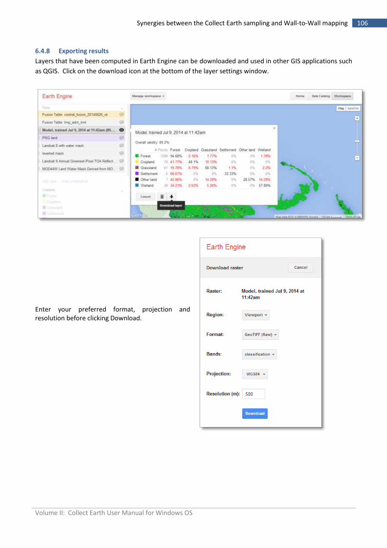
Volume II: Collect Earth User Manual for Windows OS
106 Synergies between the Collect Earth sampling and Wall-to-Wall mapping
6.4.8 Exporting results
Layers that have been computed in Earth Engine can be downloaded and used in other GIS applications such
as QGIS. Click on the download icon at the bottom of the layer settings window.
Enter your preferred format, projection and resolution before clicking Download.
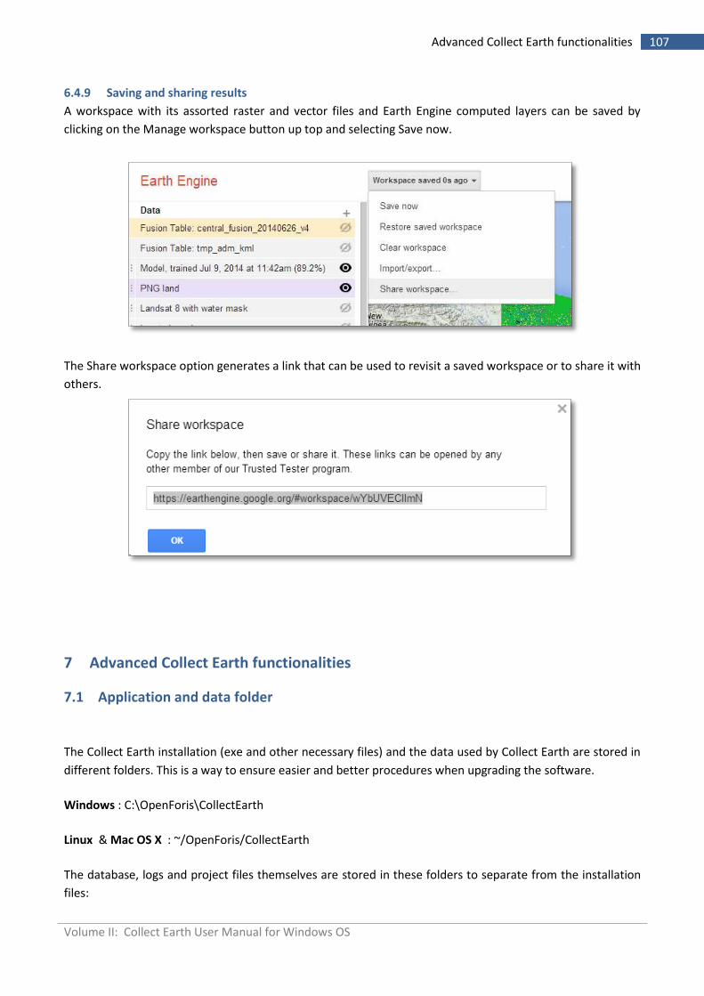
Volume II: Collect Earth User Manual for Windows OS
107 Advanced Collect Earth functionalities
6.4.9 Saving and sharing results
A workspace with its assorted raster and vector files and Earth Engine computed layers can be saved by
clicking on the Manage workspace button up top and selecting Save now.
The Share workspace option generates a link that can be used to revisit a saved workspace or to share it with
others.
7 Advanced Collect Earth functionalities
7.1 Application and data folder
The Collect Earth installation (exe and other necessary files) and the data used by Collect Earth are stored in
different folders. This is a way to ensure easier and better procedures when upgrading the software.
Windows : C:\OpenForis\CollectEarth
Linux & Mac OS X : ~/OpenForis/CollectEarth
The database, logs and project files themselves are stored in these folders to separate from the installation
files:
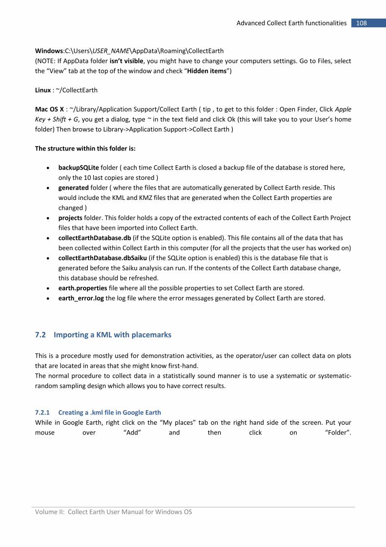
Volume II: Collect Earth User Manual for Windows OS
108 Advanced Collect Earth functionalities
Windows:C:\Users\USER_NAME\AppData\Roaming\CollectEarth
(NOTE: If AppData folder isn’t visible, you might have to change your computers settings. Go to Files, select
the “View” tab at the top of the window and check “Hidden items”)
Linux : ~/CollectEarth
Mac OS X : ~/Library/Application Support/Collect Earth ( tip , to get to this folder : Open Finder, Click Apple
Key + Shift + G, you get a dialog, type ~ in the text field and click Ok (this will take you to your User’s home
folder) Then browse to Library->Application Support->Collect Earth )
The structure within this folder is:
backupSQLite folder ( each time Collect Earth is closed a backup file of the database is stored here,
only the 10 last copies are stored )
generated folder ( where the files that are automatically generated by Collect Earth reside. This
would include the KML and KMZ files that are generated when the Collect Earth properties are
changed )
projects folder. This folder holds a copy of the extracted contents of each of the Collect Earth Project
files that have been imported into Collect Earth.
collectEarthDatabase.db (if the SQLite option is enabled). This file contains all of the data that has
been collected within Collect Earth in this computer (for all the projects that the user has worked on)
collectEarthDatabase.dbSaiku (if the SQLite option is enabled) this is the database file that is
generated before the Saiku analysis can run. If the contents of the Collect Earth database change,
this database should be refreshed.
earth.properties file where all the possible properties to set Collect Earth are stored.
earth_error.log the log file where the error messages generated by Collect Earth are stored.
7.2 Importing a KML with placemarks
This is a procedure mostly used for demonstration activities, as the operator/user can collect data on plots
that are located in areas that she might know first-hand.
The normal procedure to collect data in a statistically sound manner is to use a systematic or systematic-
random sampling design which allows you to have correct results.
7.2.1 Creating a .kml file in Google Earth
While in Google Earth, right click on the “My places” tab on the right hand side of the screen. Put your
mouse over “Add” and then click on “Folder”.
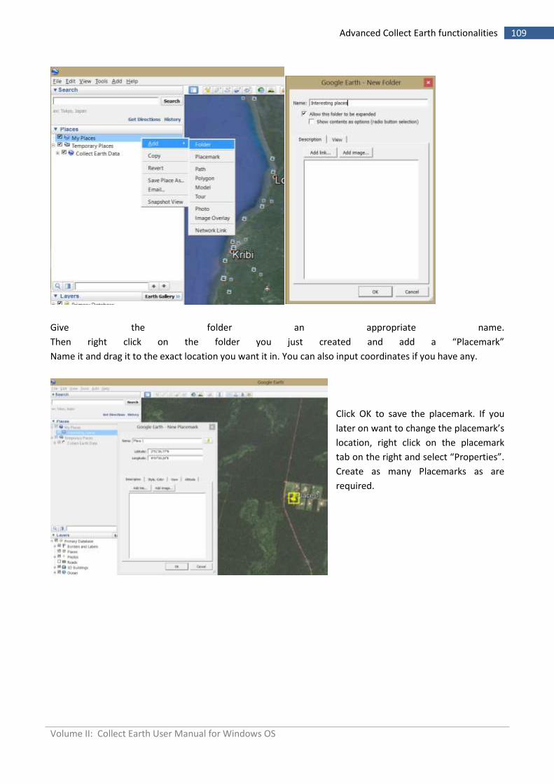
Volume II: Collect Earth User Manual for Windows OS
109 Advanced Collect Earth functionalities
Give the folder an appropriate name.
Then right click on the folder you just created and add a “Placemark”
Name it and drag it to the exact location you want it in. You can also input coordinates if you have any.
Click OK to save the placemark. If you
later on want to change the placemark’s
location, right click on the placemark
tab on the right and select “Properties”.
Create as many Placemarks as are
required.
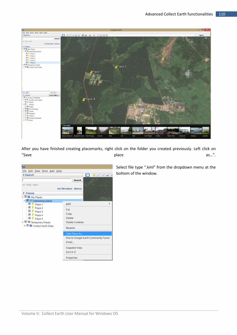
Volume II: Collect Earth User Manual for Windows OS
110 Advanced Collect Earth functionalities
After you have finished creating placemarks, right click on the folder you created previously. Left click on
“Save place as…”.
Select file type “.kml” from the dropdown menu at the
bottom of the window.
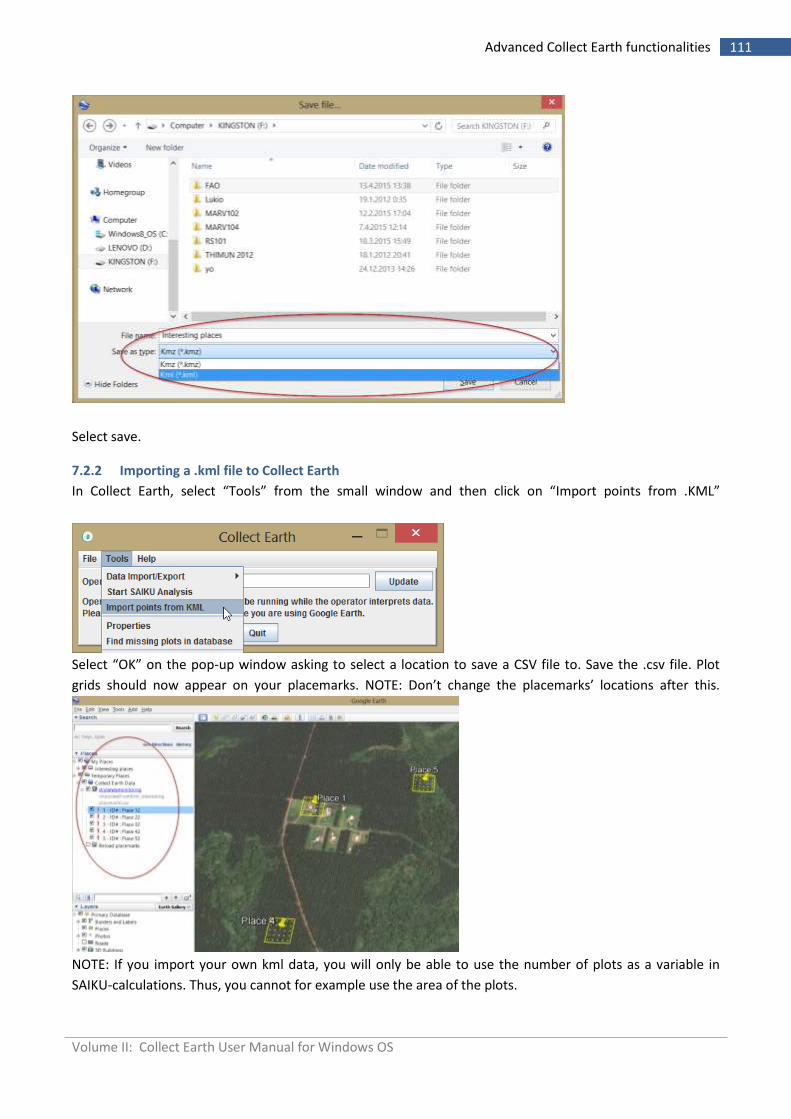
Volume II: Collect Earth User Manual for Windows OS
111 Advanced Collect Earth functionalities
Select save.
7.2.2 Importing a .kml file to Collect Earth
In Collect Earth, select “Tools” from the small window and then click on “Import points from .KML”
Select “OK” on the pop-up window asking to select a location to save a CSV file to. Save the .csv file. Plot
grids should now appear on your placemarks. NOTE: Don’t change the placemarks’ locations after this.
NOTE: If you import your own kml data, you will only be able to use the number of plots as a variable in
SAIKU-calculations. Thus, you cannot for example use the area of the plots.
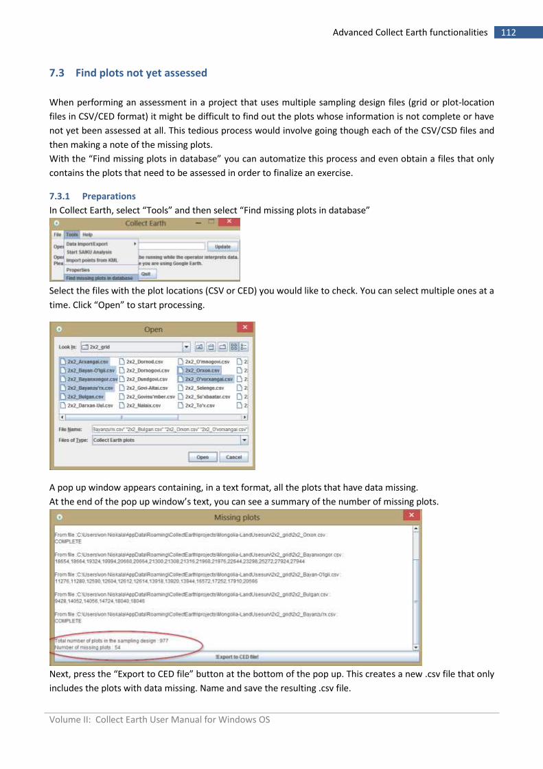
Volume II: Collect Earth User Manual for Windows OS
112 Advanced Collect Earth functionalities
7.3 Find plots not yet assessed
When performing an assessment in a project that uses multiple sampling design files (grid or plot-location
files in CSV/CED format) it might be difficult to find out the plots whose information is not complete or have
not yet been assessed at all. This tedious process would involve going though each of the CSV/CSD files and
then making a note of the missing plots.
With the “Find missing plots in database” you can automatize this process and even obtain a files that only
contains the plots that need to be assessed in order to finalize an exercise.
7.3.1 Preparations
In Collect Earth, select “Tools” and then select “Find missing plots in database”
Select the files with the plot locations (CSV or CED) you would like to check. You can select multiple ones at a
time. Click “Open” to start processing.
A pop up window appears containing, in a text format, all the plots that have data missing.
At the end of the pop up window’s text, you can see a summary of the number of missing plots.
Next, press the “Export to CED file” button at the bottom of the pop up. This creates a new .csv file that only
includes the plots with data missing. Name and save the resulting .csv file.
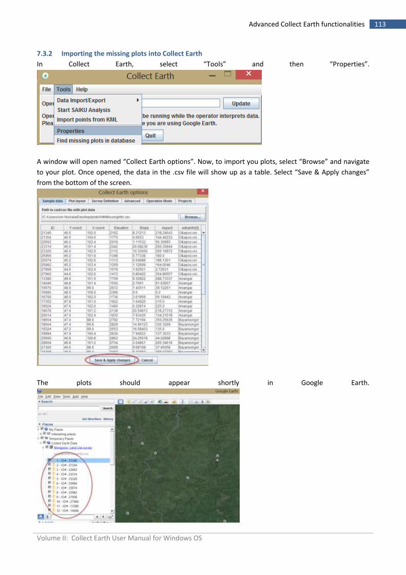
Volume II: Collect Earth User Manual for Windows OS
113 Advanced Collect Earth functionalities
7.3.2 Importing the missing plots into Collect Earth
In Collect Earth, select “Tools” and then “Properties”.
A window will open named “Collect Earth options”. Now, to import you plots, select “Browse” and navigate
to your plot. Once opened, the data in the .csv file will show up as a table. Select “Save & Apply changes”
from the bottom of the screen.
The plots should appear shortly in Google Earth.
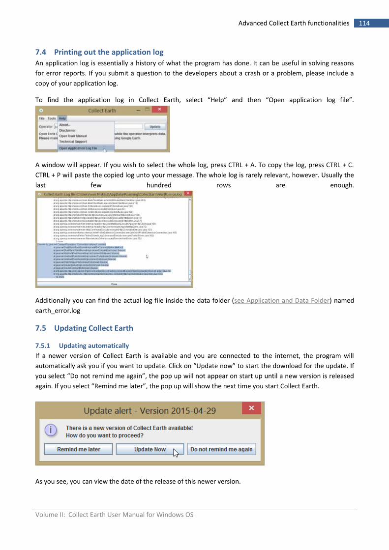
Volume II: Collect Earth User Manual for Windows OS
114 Advanced Collect Earth functionalities
7.4 Printing out the application log
An application log is essentially a history of what the program has done. It can be useful in solving reasons
for error reports. If you submit a question to the developers about a crash or a problem, please include a
copy of your application log.
To find the application log in Collect Earth, select “Help” and then “Open application log file”.
A window will appear. If you wish to select the whole log, press CTRL + A. To copy the log, press CTRL + C.
CTRL + P will paste the copied log unto your message. The whole log is rarely relevant, however. Usually the
last few hundred rows are enough.
Additionally you can find the actual log file inside the data folder (see Application and Data Folder) named
earth_error.log
7.5 Updating Collect Earth
7.5.1 Updating automatically
If a newer version of Collect Earth is available and you are connected to the internet, the program will
automatically ask you if you want to update. Click on “Update now” to start the download for the update. If
you select “Do not remind me again”, the pop up will not appear on start up until a new version is released
again. If you select “Remind me later”, the pop up will show the next time you start Collect Earth.
As you see, you can view the date of the release of this newer version.
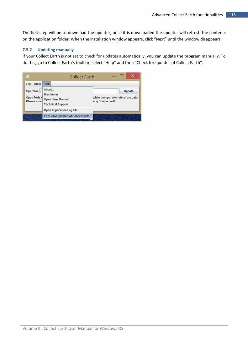
Volume II: Collect Earth User Manual for Windows OS
115 Advanced Collect Earth functionalities
The first step will be to download the updater, once it is downloaded the updater will refresh the contents
on the application folder. When the installation window appears, click “Next” until the window disappears.
7.5.2 Updating manually
If your Collect Earth is not set to check for updates automatically, you can update the program manually. To
do this; go to Collect Earth’s toolbar, select “Help” and then “Check for updates of Collect Earth”.
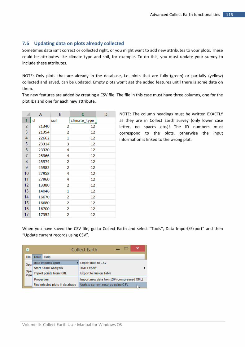
Volume II: Collect Earth User Manual for Windows OS
116 Advanced Collect Earth functionalities
7.6 Updating data on plots already collected Sometimes data isn’t correct or collected right, or you might want to add new attributes to your plots. These
could be attributes like climate type and soil, for example. To do this, you must update your survey to
include these attributes.
NOTE: Only plots that are already in the database, i.e. plots that are fully (green) or partially (yellow)
collected and saved, can be updated. Empty plots won’t get the added features until there is some data on
them.
The new features are added by creating a CSV file. The file in this case must have three columns, one for the
plot IDs and one for each new attribute.
NOTE: The column headings must be written EXACTLY
as they are in Collect Earth survey (only lower case
letter, no spaces etc.)! The ID numbers must
correspond to the plots, otherwise the input
information is linked to the wrong plot.
When you have saved the CSV file, go to Collect Earth and select “Tools”, Data Import/Export” and then
“Update current records using CSV”.
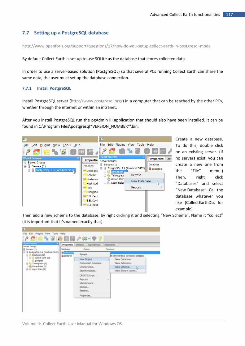
Volume II: Collect Earth User Manual for Windows OS
117 Advanced Collect Earth functionalities
7.7 Setting up a PostgreSQL database
http://www.openforis.org/support/questions/17/how-do-you-setup-collect-earth-in-postgresql-mode
By default Collect Earth is set up to use SQLite as the database that stores collected data.
In order to use a server-based solution (PostgreSQL) so that several PCs running Collect Earth can share the
same data, the user must set up the database connection.
7.7.1 Install PostgreSQL
Install PostgreSQL server (http://www.postgresql.org/) in a computer that can be reached by the other PCs,
whether through the internet or within an intranet.
After you install PostgreSQL run the pgAdmin III application that should also have been installed. It can be
found in C:\Program Files\postgresql*VERSION_NUMBER*\bin.
Create a new database.
To do this, double click
on an existing server. (If
no servers exist, you can
create a new one from
the “File” menu.)
Then, right click
“Databases” and select
“New Database”. Call the
database whatever you
like (CollectEarthDb, for
example).
Then add a new schema to the database, by right clicking it and selecting “New Schema”. Name it “collect”
(it is important that it’s named exactly that).
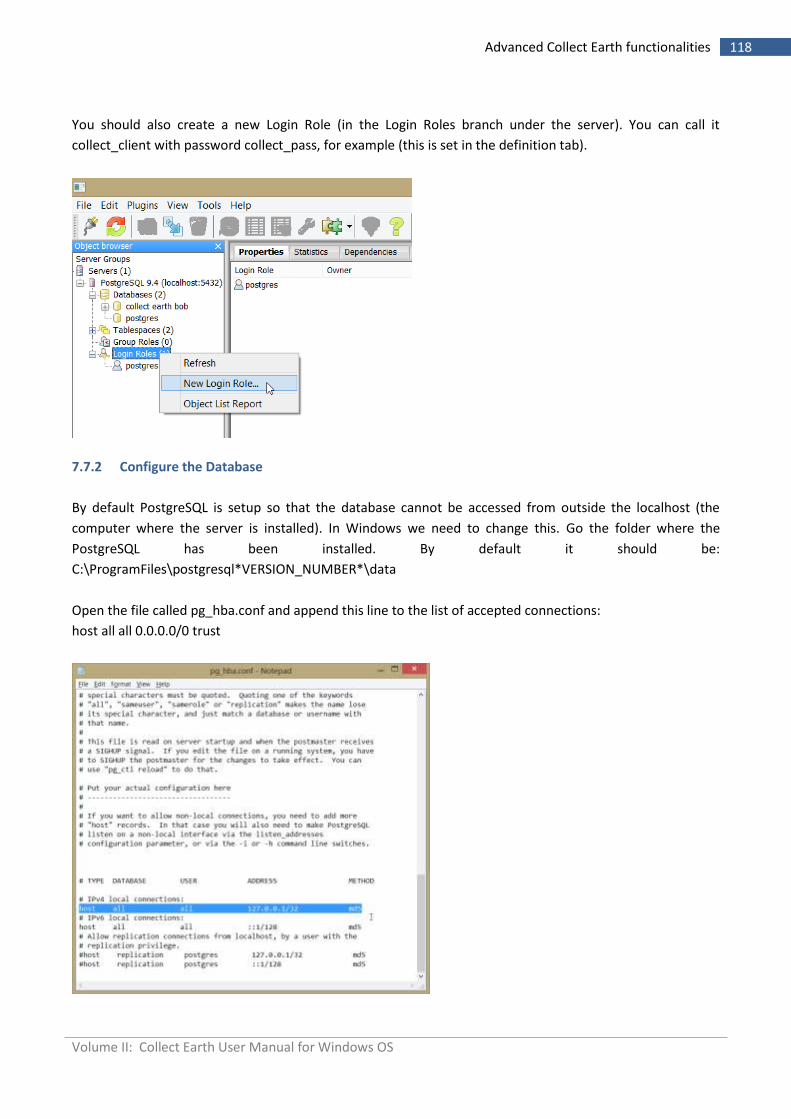
Volume II: Collect Earth User Manual for Windows OS
118 Advanced Collect Earth functionalities
You should also create a new Login Role (in the Login Roles branch under the server). You can call it
collect_client with password collect_pass, for example (this is set in the definition tab).
7.7.2 Configure the Database
By default PostgreSQL is setup so that the database cannot be accessed from outside the localhost (the
computer where the server is installed). In Windows we need to change this. Go the folder where the
PostgreSQL has been installed. By default it should be:
C:\ProgramFiles\postgresql*VERSION_NUMBER*\data
Open the file called pg_hba.conf and append this line to the list of accepted connections:
host all all 0.0.0.0/0 trust
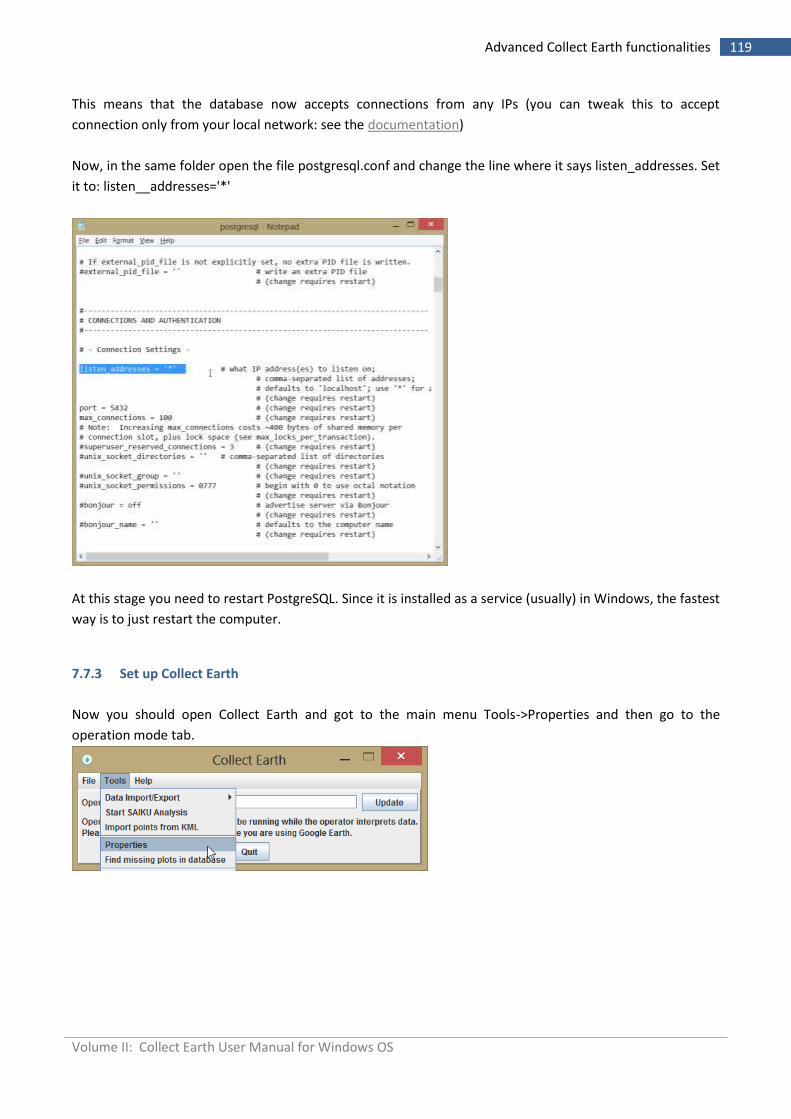
Volume II: Collect Earth User Manual for Windows OS
119 Advanced Collect Earth functionalities
This means that the database now accepts connections from any IPs (you can tweak this to accept
connection only from your local network: see the documentation)
Now, in the same folder open the file postgresql.conf and change the line where it says listen_addresses. Set
it to: listen__addresses='*'
At this stage you need to restart PostgreSQL. Since it is installed as a service (usually) in Windows, the fastest
way is to just restart the computer.
7.7.3 Set up Collect Earth
Now you should open Collect Earth and got to the main menu Tools->Properties and then go to the
operation mode tab.
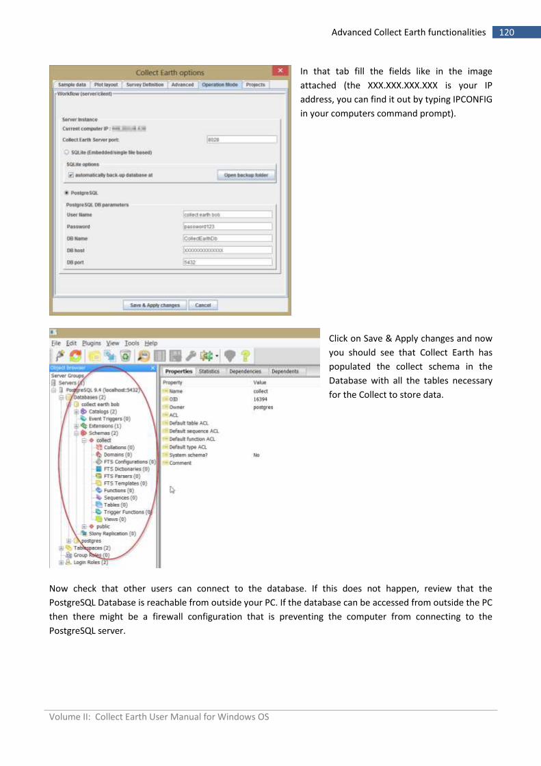
Volume II: Collect Earth User Manual for Windows OS
120 Advanced Collect Earth functionalities
In that tab fill the fields like in the image
attached (the XXX.XXX.XXX.XXX is your IP
address, you can find it out by typing IPCONFIG
in your computers command prompt).
Click on Save & Apply changes and now
you should see that Collect Earth has
populated the collect schema in the
Database with all the tables necessary
for the Collect to store data.
Now check that other users can connect to the database. If this does not happen, review that the
PostgreSQL Database is reachable from outside your PC. If the database can be accessed from outside the PC
then there might be a firewall configuration that is preventing the computer from connecting to the
PostgreSQL server.
Volume II: Collect Earth User Manual for Windows OS
121 Advanced Collect Earth functionalities
i Add two countries whose suggestions or participation in the project have been particularly useful for improving Collect Earth ii Add names of individuals who have made valuable contributions to the development of Collect Earth and/or this user
manual