Visualizing Field-Measured Seismic DataTung-Ju Hsieh∗

National Taipei University of TechnologyCheng-Kai Chen†

University of California, DavisKwan-Liu Ma‡

University of California, Davis

ABSTRACT

This paper presents visualization of field-measured, time-varyingmultidimensional earthquake accelerograph readings. Direct vol-ume rendering is used to depict the space-time relationships ofseismic readings collected from sensor stations in an intuitive waysuch that the progress of seismic wave propagation of an earthquakeevent can be directly observed. The resulting visualization revealsthe sequence of seismic wave initiation, propagation, attenuationover time, and energy releasing events. We provide a case study onthe magnitude scale Mw 7.6 Chi-Chi earthquake in Taiwan, whichis the most thoroughly recorded earthquake event ever in the his-tory. More than 400 stations recorded this event, and the readingsfrom this event increased global strong-motion records five folds.Each station measured east-west, north-south, and vertical com-ponent of acceleration for approximately 90 seconds. The sensornetwork released the initial raw data within minutes after the Chi-Chi mainshock. It is essential to have a visualization system forfast data exploring and analyzing, offering crucial visual analyti-cal information for scientists to make quick judgments. Raw datarequires preprocessing before it can be rendered. We generated asequence of ground-motion wave-field maps of 350× 200 regulargrid covers the entire Taiwan island from the sensor network read-ings. The result is a total of 1000 ground-motion wave-field mapswith 0.1 second interval, forming a 1000×350×200 volume dataset. We show that visualizing the time-varying component of thedata spatially uncovers the changing features hidden in the data.

Index Terms: I.3.8 [Computer Graphics]: Applications; I.3.3[Computer Graphics]: Picture/Image Generation

1 INTRODUCTION

In many areas of seismological science and earthquake engineering,the multi-channel and time-varying components add difficulties indata exploration. The field-measured data collected from an ac-celerograph instrumentation can contain thousands of time stepsand each time step has readings from three channels (east-west,north-south, vertical). The collection of readings from a sensor net-work requires a huge amount of storage which creates challengesfor subsequent analysis. Without proper tools, it is difficult to un-cover and observe the complex physical and mechanical phenom-ena contained in these data sets. In addition, the release of sen-sor network readings is crucial for providing needed information inearthquake hazard response, damage assessment, and rescue plan-ning. In the long term, the collection of sensor network readingsserves as a statistical database for estimating earthquake occurrenceprobability and establishing safety factor design codes for civil in-frastructure and buildings. These earthquake resistant structural de-sign specifications are based on the history of earthquake records,and structural engineers rely on them to design proper structural el-ements of a building. If the safety factor is set too high, it increases

∗e-mail: tjh@csie.ntut.edu.tw†e-mail:ckchen@ucdavis.edu‡e-mail:ma@cs.ucdavis.edu

121 E

22 N

23 N

24 N

25 N

122 E120 E

(a) (b) 0 (gal) >400

Acceleration

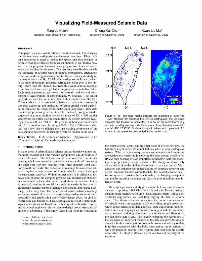
Figure 1: (a) The blue marks indicate the locations of over 446TSMIP stations that recorded the Chi-Chi earthquake; the red crossindicates the location of epicenter. It is so far the most thoroughlyrecorded earthquake ever. (b) Snapshots of acceleration wave-fieldmap at UTC 17:47:50. Surface fitting with biharmonic operator in 2Dis used to complete the unsampled areas on the map.

the constructional costs. On the other hand, if it is set too low, thebuildings might suffer structural failures when a large earthquakestrikes. When a large earthquake occurs, scientists and engineersare particularly interested in studying the peak ground acceleration(PGA) map because it is an important influencing factor in choos-ing the proper safety design standards. The ability to interactivelydetect and explore the hidden phenomena in data is essential. Visu-alization can enhance the understanding of complex behavior anddetect important features within the data. It is desirable for a visual-ization system to provide the functionality for changing viewpointsand modifying color mappings and classification functions at an in-teractive rate.

This paper presents a study of a unique field-measured seismicdata set, capturing 1999 Chi-Chi earthquake in Taiwan, using acustom-made interactive volume visualization system. Unlike con-ventional approaches, we treat time-varying 2D data as volumedata. This allows scientists to capture the entire time evolutionof seismic waves propagation in 3D, providing unique properties,which draws attention to data analysis. Data exploration function-alities such as changing viewpoints, zooming in and out, and inter-active volume rendering of seismic data allows us to fully observethe data from start to end. This greatly enhances the perception ofthe sequence of important features in the data and provides uniqueclues for further investigations. When the volume rendering of datais further augmented with the PGA information, the directions ofwave propagation emerge from volume data and become clearlyobservable. It is highly affected by the mechanical property of themedium.

2 EARTHQUAKE MONITORING

Earthquake is one of the most devastating forces in nature. Instru-mentation, observation, and archiving of strong ground motionsprovide valuable data that holds the key to do analysis and thuscan aid in earthquake hazard mitigation and understanding of seis-mic wave propagation. The Taiwan Strong-Motion InstrumentationProgram (TSMIP) completed the installation of strong-motion ac-celerographs in 1996 before the Chi-Chi earthquake occurred. Thestrong-motion sensors record the dynamic surface motion. Thereare approximately 700 digital accelerographs in free-field stations,and more than 50 real-time seismic arrays installed in buildings andbridges. With 3 km station spacing of free-field accelerographs inurban area, Taiwan has the densest strong-motion instrument net-work in the world [20] compared to 25 km spacing of K-net strongmotion seismograph network in Japan [15]. Typical accelerographshave ±2 g scale, 200 or higher sampling rate, 16-bit precision, and20 second pre-event recording with a Global Positioning System(GPS) receiver that can be used to synchronize the internal clock toCoordinated Universal Time (UTC) [23].

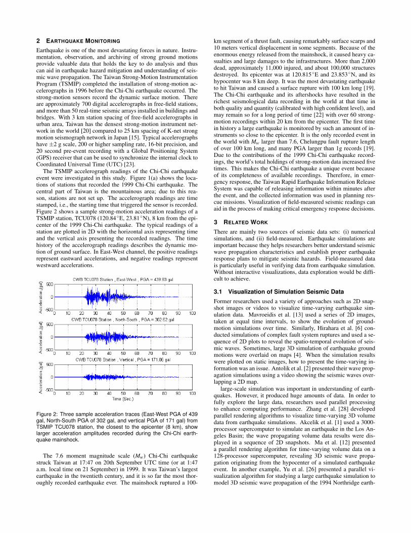
The TSMIP accelerograph readings of the Chi-Chi earthquakeevent were investigated in this study. Figure 1(a) shows the loca-tions of stations that recorded the 1999 Chi-Chi earthquake. Thecentral part of Taiwan is the mountainous area; due to this rea-son, stations are not set up. The accelerograph readings are timestamped, i.e., the starting time that triggered the sensor is recorded.Figure 2 shows a sample strong-motion acceleration readings of aTSMIP station, TCU078 (120.84◦E, 23.81◦N), 8 km from the epi-center of the 1999 Chi-Chi earthquake. The typical readings of astation are plotted in 2D with the horizontal axis representing timeand the vertical axis presenting the recorded readings. The timehistory of the accelerograph readings describes the dynamic mo-tion of ground surface. In East-West channel, the positive readingsrepresent eastward accelerations, and negative readings representwestward accelerations.

Figure 2: Three sample acceleration traces (East-West PGA of 439gal, North-South PGA of 302 gal, and vertical PGA of 171 gal) fromTSMIP TCU078 station, the closest to the epicenter (8 km), showlarger acceleration amplitudes recorded during the Chi-Chi earth-quake mainshock.

The 7.6 moment magnitude scale (Mw) Chi-Chi earthquakestruck Taiwan at 17:47 on 20th September UTC time (or at 1:47a.m. local time on 21 September) in 1999. It was Taiwan’s largestearthquake in the twentieth century, and it is so far the most thor-oughly recorded earthquake ever. The mainshock ruptured a 100-

km segment of a thrust fault, causing remarkably surface scarps and10 meters vertical displacement in some segments. Because of theenormous energy released from the mainshock, it caused heavy ca-sualties and large damages to the infrastructures. More than 2,000dead, approximately 11,000 injured, and about 100,000 structuresdestroyed. Its epicenter was at 120.815◦E and 23.853◦N, and itshypocenter was 8 km deep. It was the most devastating earthquaketo hit Taiwan and caused a surface rupture with 100 km long [19].The Chi-Chi earthquake and its aftershocks have resulted in therichest seismological data recording in the world at that time inboth quality and quantity (calibrated with high confident level), andmay remain so for a long period of time [22] with over 60 strong-motion recordings within 20 km from the epicenter. The first timein history a large earthquake is monitored by such an amount of in-struments so close to the epicenter. It is the only recorded event inthe world with Mw larger than 7.6, Chelungpu fault rupture lengthof over 100 km long, and many PGA larger than 1g records [19].Due to the contributions of the 1999 Chi-Chi earthquake record-ings, the world’s total holdings of strong-motion data increased fivetimes. This makes the Chi-Chi earthquake a unique event becauseof its completeness of available recordings. Therefore, in emer-gency response, the Taiwan Rapid Earthquake Information ReleaseSystem was capable of releasing information within minutes afterthe event, and the collected information was used in planning res-cue missions. Visualization of field-measured seismic readings canaid in the process of making critical emergency response decisions.

3 RELATED WORK

There are mainly two sources of seismic data sets: (i) numericalsimulations, and (ii) field-measured. Earthquake simulations areimportant because they helps researchers better understand seismicwave propagation characteristics and establish proper earthquakeresponse plans to mitigate seismic hazards. Field-measured datais particularly useful in verifying data from earthquake simulation.Without interactive visualizations, data exploration would be diffi-cult to achieve.

3.1 Visualization of Simulation Seismic DataFormer researchers used a variety of approaches such as 2D snap-shot images or videos to visualize time-varying earthquake sim-ulation data. Mavroeidis et al. [13] used a series of 2D images,taken at equal time intervals, to show the evolution of ground-motion simulations over time. Similarly, Hirahara et al. [6] con-ducted simulations of complex fault system ruptures and used a se-quence of 2D plots to reveal the spatio-temporal evolution of seis-mic waves. Sometimes, large 3D simulation of earthquake groundmotions were overlaid on maps [4]. When the simulation resultswere plotted on static images, how to present the time-varying in-formation was an issue. Antolik et al. [2] presented their wave prop-agation simulations using a video showing the seismic waves over-lapping a 2D map.

large-scale simulation was important in understanding of earth-quakes. However, it produced huge amounts of data. In order tofully explore the large data, researchers used parallel processingto enhance computing performance. Zhang et al. [28] developedparallel rendering algorithms to visualize time-varying 3D volumedata from earthquake simulations. Akcelik et al. [1] used a 3000-processor supercomputer to simulate an earthquake in the Los An-geles Basin; the wave propagating volume data results were dis-played in a sequence of 2D snapshots. Ma et al. [12] presenteda parallel rendering algorithm for time-varying volume data on a128-processor supercomputer, revealing 3D seismic wave propa-gation originating from the hypocenter of a simulated earthquakeevent. In another example, Yu et al. [26] presented a parallel vi-sualization algorithm for studying a large earthquake simulation tomodel 3D seismic wave propagation of the 1994 Northridge earth-

quake. Chourasia et al. [5] presented a cast study of visualizinglarge-scale earthquake simulations on a supercomputer, encodingthe rendered images into animations. These works dealt with dataof simulation results. This decomposition of simulation and visual-ization became undesired as the large simulations moved into teras-cale and petascale. In contrast, Tu et al. [24] presented another typeof system, which simulation components and visualization weretightly coupled together so that real-time rendering of simulationdata was made possible. Chopra et al. [3] presented a visualizationwork of earthquake simulation data to enhance collaboration be-tween structural engineers, seismologists, and computer scientistsin an immersive virtual environment to present the simulation databetter. These simulations provide a mean to better understand theearthquake, however, it is also important to verify simulation resultswith field-collected seismic data. Komatitsch et al. [7] conducted aglobal-scale simulation of seismic wave propagation and superim-posed the simulation data over field-measured waveforms data.

3.2 Visualization of Field-Measured Seismic Data

Large field-measured seismic data sets posed significant challengesfor processing and analyzing. Yuen et al. [27] presented a web-based system for visualizing seismic data in a grid environment. Aconventional approach to analyze the field-collected data sets wasto study earthquake induced effects as time histories by plottingand comparing discrete waveforms. Wolfe et al. [25] presented avisualization system for examining the seismic volume data gener-ated from ultrasound reflections, looking for high-amplitude seis-mic events through a synoptic view of the interior. Tools were de-veloped for interpreting and illustrating 2D slices of seismic vol-umetric reflection data [16]. Nayak et al. [14] used 3D glyphs,graphics primitives or symbols with various geometric and color at-tributes, to represent the measured seismic data. These glyphs wererendered in real time and combined with a 3D topography terrainmap. In particular, 3D visualization can provide visual clues viaan intuitive representation of the time-varying information that isdifficult to represent with traditional 2D techniques. Visual analyt-ics tools are aimed to aid the process of analyzing field-measuredseismic data sets and leading to new discoveries. When properlygeoreferenced and treated, seismic data sets can be presented in anatural form that facilitates the understanding of governing mech-anisms. For example, the peak ground-motion map can be com-puted from sensor readings of an earthquake. It is a static mapshowing the recorded peak values of different locations during anearthquake.

A series of 2D ground-motion wave-field maps over time can begenerated from the field-measured records of an earthquake event.A single ground-motion wave-field map only shows a snapshot ofacceleration readings at a particular time. In contrast, a sequence ofground-motion wave-field maps show the initiation and propagationprogress of ground motions. These wave-filed maps can be used togenerate a video clip for further analysis. From the playback of avideo clip, the time history of ground motions can be observed. Us-ing the sensor network readings from the 1999 Chi-Chi earthquake,Shin and Teng [19] produced a video of 100 time frames, presentedat one frame per second, showing the ground motions from startto finish throughout the island. In their approach, each station wastreated as a pixel and interpolation was used to fill the empty pixelsbetween stations. In addition, they used a low-pass filter to trim thehigh frequency portion of the signals to avoid breaking up wave-field maps. From the playback of the video, major energy releaseswere determined in time and space. A major energy release was de-fined as an event that emerged at the surface in an area of nearly 10km in radius with accelerations of 350 gal and larger. They pointedout that major energy releases happened at 11, 14, 15, 16, 18, 19,20, 21, 23, 27, 29, 30, 32, 34, 43, and 50 seconds from origin time.Some of the major energy releases were from adjacent active faults

triggered by the bursts of extensive energy releases of the main-shock. From the examination of the time-space relationship of themajor energy releases, they further concluded that there was no par-ticular order with which these energy releases took place, Shin andTeng called this type of rupture jumping dislocations. Stress fieldwas irregular along the fault zones; dislocation occurred where thestress concentration exceeded the rock strength.

In order to fully present the time history of the field-measuredground motions, new approaches are needed to provide a spatiallyand temporally anchored, visual representation of the earthquakephenomenon. Different from previous methods of using a video toshow the time-history of the sensor readings, Romero Summet [17]presented a system to visualize the entire contents of a video bystacking frames up in sequence. This approach enabled longitudi-nal analysis of the aggregation of contents in a video. In a similarway, a sequence of wave-filed maps can be stacked up in 3D. In thispaper, a new approach was presented to visualize the world’s mostcomplete field-measured earthquake ground-motion readings. Vol-ume rendering techniques were used to examine the unstructuredtime-varying seismic data. Compared to conventional approaches,volume rendering provided new perspectives to look at the data.These visual paradigms provided an enhanced understanding of thefield-measured seismic data. When coupled with feature extractingtechniques, interactive visualization played a crucial role in explor-ing the seismic data.

4 VISUALIZATION OF ACCELEROGRAPH READINGS

Since most of the TSMIP accelerographs have absolute timingtuned with GPS receiver timing and all stations have accurate rela-tive timing, a common time reference was inputted into all records.The seismic sensor readings from the Chi-Chi earthquake was usedto generate a sequence of ground-motion wave-field maps. Be-cause the TSMIP sensor network has the densest station distribu-tion in the world, the resolution produced from the raw data wasenhanced significantly, showing more completed ground-motionwave-field maps. Our seismologist collaborator suggested that sur-face fitting [18] should be used to interpolate the regular grid map.It models a surface (fits grid values) from scattered data in theform of z(x,y) for each channel. Using biharmonic operator in2D achieves minimum curvature interpolation of irregularly spacedsampled points, so the result surface always passes through the sam-pled data points. Since scientists are mostly interested in studyingenergy, absolute values are used for the readings of the three chan-nels in this study. Figure 1(b) shows a snapshot of ground-motionwave-field map (regular grid of resolution 350×200) generated byusing surface fitting. Each pixel presents an area of approximately1 km2. The color transfer function input is calculated from the am-plitude of the three channels (east-west, north-south, vertical). Theregion of over 400 gal acceleration is indicated in red, while theregion of lower acceleration is in blue.

In this research, a total of 1000 ground-motion wave-field mapswith a 0.1 second interval are generated from the sensor networkreadings of the 1999 Chi-Chi earthquake. These maps are stackedup in sequence to form a 1000×350×200 volume data to presentthe time-varying information in spatial form. This approach allowsthe time-varying information to be presented spatially. Volume ren-dering is used because it provides a means to present the seismicwave propagation sequence of an earthquake over time, allowingseismologists to observe the seismic wave propagation at a glance.Volume rendering is particularly useful in presenting the spatio-temporal relationship of the energy releases in volume data. Thepurpose is to discover the size and shape of the energy releasesthrough color-coding the volume data.

4.1 Direct Volume Rendering of Wave-Field VolumeDirect volume rendering using ray casting is a well-developed ren-dering technique that can visualize the internal structure of the 3Dvolume data. It displays the data directly without constructing geo-metric primitives to the samples first. Modern programmable GPUsaccelerates ray casting, making volume rendering more usable andattractive. Formerly, Kruger and Westermann [8] presented a GPU-based ray caster implemented in the fragment shader with earlytermination and empty space skipping features. Another exam-ple, Lum et al. [11] presented a GPU-based volume rendering tech-nique for interactive visualization of the time-varying volume data.In their design, a palette-based decoding technique was developedto fully utilize the texture mapping capability. The incrementalsubrange integration was proposed [10] to speed up pre-integratedvolume rendering, which can minimize artifacts caused by regularsampling and generate high-quality visualization. A single-pass raycaster was developed by [21] to perform pre-integrated direct vol-ume rendering.

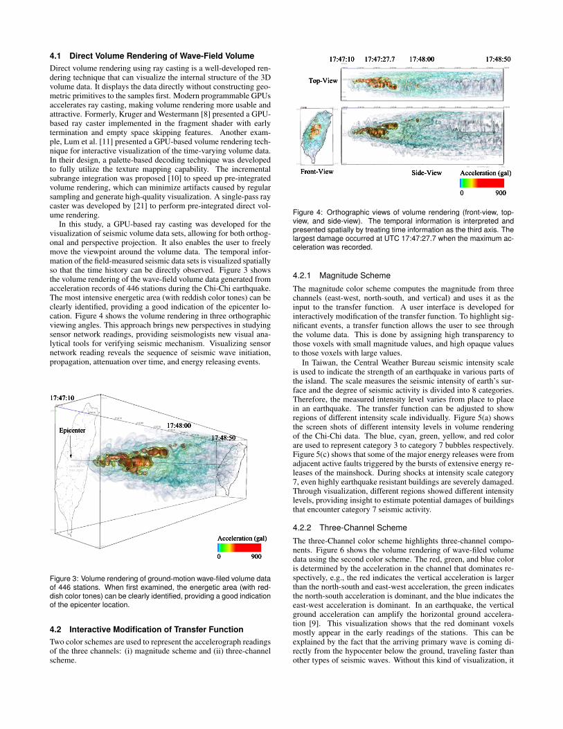
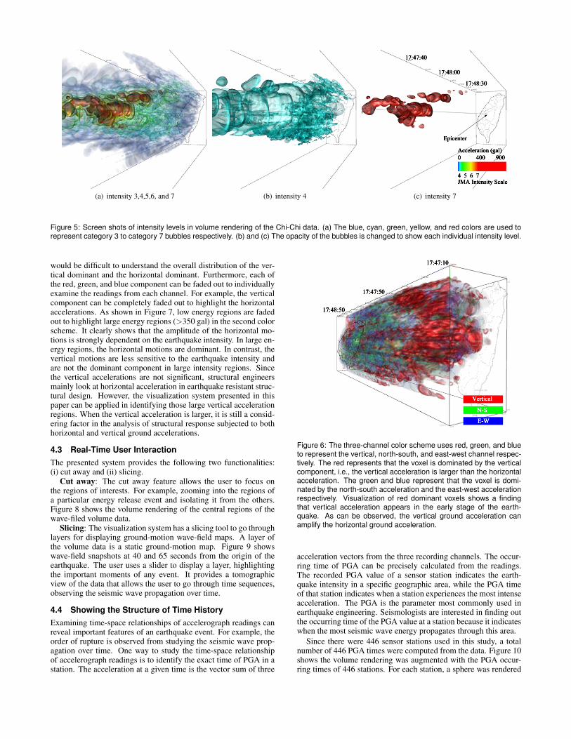
In this study, a GPU-based ray casting was developed for thevisualization of seismic volume data sets, allowing for both orthog-onal and perspective projection. It also enables the user to freelymove the viewpoint around the volume data. The temporal infor-mation of the field-measured seismic data sets is visualized spatiallyso that the time history can be directly observed. Figure 3 showsthe volume rendering of the wave-field volume data generated fromacceleration records of 446 stations during the Chi-Chi earthquake.The most intensive energetic area (with reddish color tones) can beclearly identified, providing a good indication of the epicenter lo-cation. Figure 4 shows the volume rendering in three orthographicviewing angles. This approach brings new perspectives in studyingsensor network readings, providing seismologists new visual ana-lytical tools for verifying seismic mechanism. Visualizing sensornetwork reading reveals the sequence of seismic wave initiation,propagation, attenuation over time, and energy releasing events.

Epicenter

Acceleration (gal)

17:47:10

17:48:00

17:48:50

0 900

Figure 3: Volume rendering of ground-motion wave-filed volume dataof 446 stations. When first examined, the energetic area (with red-dish color tones) can be clearly identified, providing a good indicationof the epicenter location.

4.2 Interactive Modification of Transfer FunctionTwo color schemes are used to represent the accelerograph readingsof the three channels: (i) magnitude scheme and (ii) three-channelscheme.

Acceleration (gal)

0 900

Front-View Side-View

Top-View

17:47:10 17:48:00 17:48:5017:47:27.7

Figure 4: Orthographic views of volume rendering (front-view, top-view, and side-view). The temporal information is interpreted andpresented spatially by treating time information as the third axis. Thelargest damage occurred at UTC 17:47:27.7 when the maximum ac-celeration was recorded.

4.2.1 Magnitude Scheme

The magnitude color scheme computes the magnitude from threechannels (east-west, north-south, and vertical) and uses it as theinput to the transfer function. A user interface is developed forinteractively modification of the transfer function. To highlight sig-nificant events, a transfer function allows the user to see throughthe volume data. This is done by assigning high transparency tothose voxels with small magnitude values, and high opaque valuesto those voxels with large values.

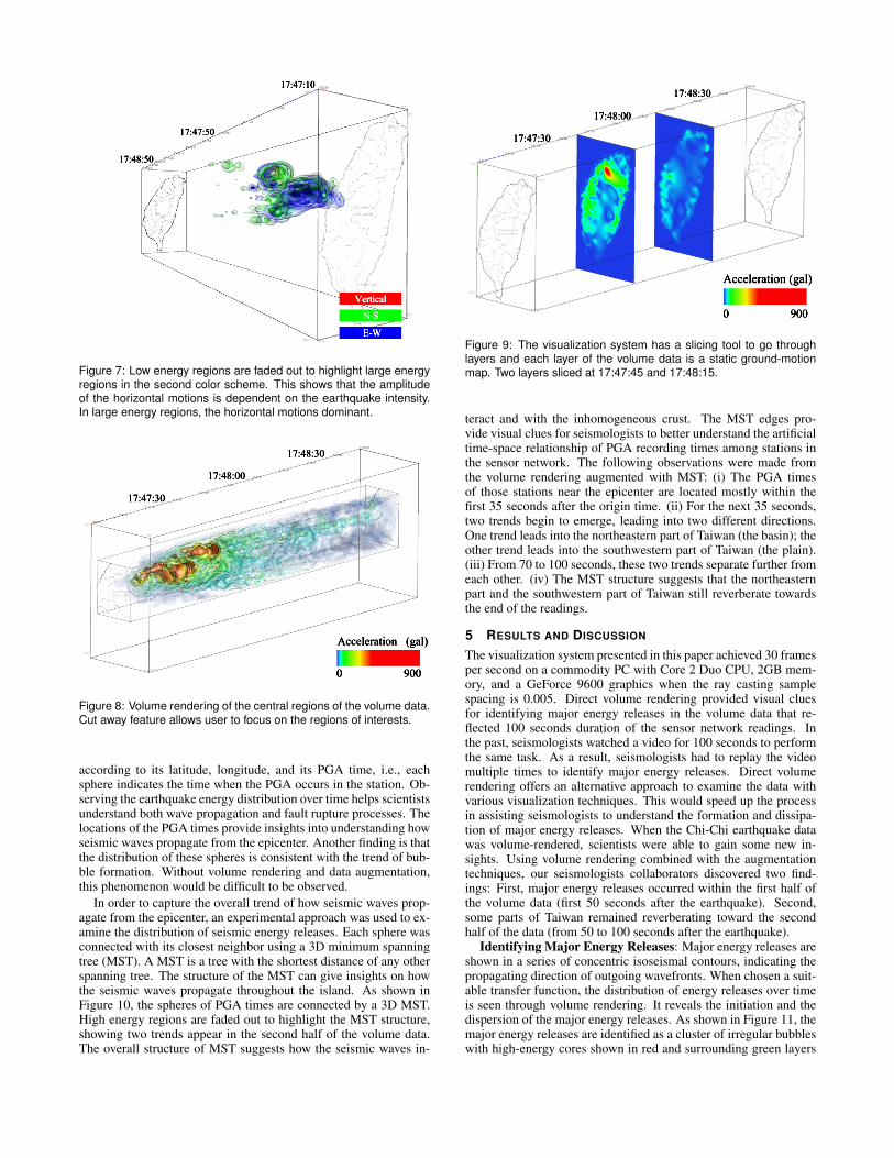
In Taiwan, the Central Weather Bureau seismic intensity scaleis used to indicate the strength of an earthquake in various parts ofthe island. The scale measures the seismic intensity of earth’s sur-face and the degree of seismic activity is divided into 8 categories.Therefore, the measured intensity level varies from place to placein an earthquake. The transfer function can be adjusted to showregions of different intensity scale individually. Figure 5(a) showsthe screen shots of different intensity levels in volume renderingof the Chi-Chi data. The blue, cyan, green, yellow, and red colorare used to represent category 3 to category 7 bubbles respectively.Figure 5(c) shows that some of the major energy releases were fromadjacent active faults triggered by the bursts of extensive energy re-leases of the mainshock. During shocks at intensity scale category7, even highly earthquake resistant buildings are severely damaged.Through visualization, different regions showed different intensitylevels, providing insight to estimate potential damages of buildingsthat encounter category 7 seismic activity.

4.2.2 Three-Channel Scheme

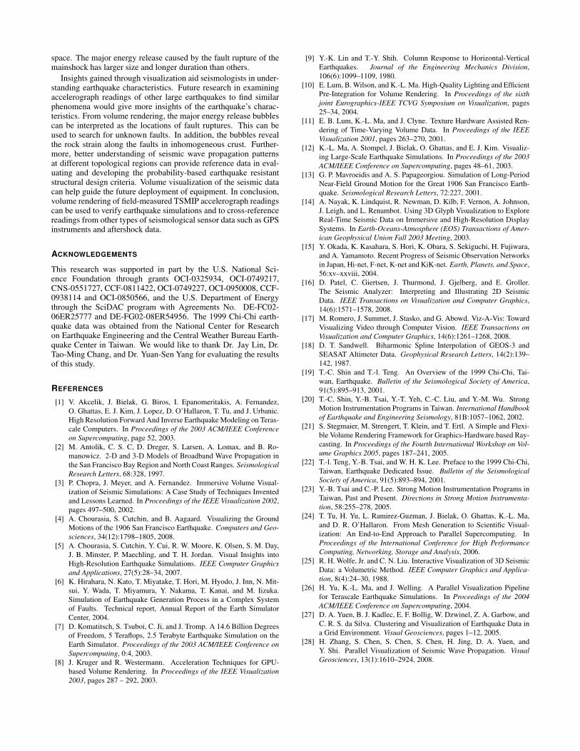
The three-Channel color scheme highlights three-channel compo-nents. Figure 6 shows the volume rendering of wave-filed volumedata using the second color scheme. The red, green, and blue coloris determined by the acceleration in the channel that dominates re-spectively, e.g., the red indicates the vertical acceleration is largerthan the north-south and east-west acceleration, the green indicatesthe north-south acceleration is dominant, and the blue indicates theeast-west acceleration is dominant. In an earthquake, the verticalground acceleration can amplify the horizontal ground accelera-tion [9]. This visualization shows that the red dominant voxelsmostly appear in the early readings of the stations. This can beexplained by the fact that the arriving primary wave is coming di-rectly from the hypocenter below the ground, traveling faster thanother types of seismic waves. Without this kind of visualization, it

(a) intensity 3,4,5,6, and 7 (b) intensity 4

JMA Intensity Scale

Epicenter

17:47:40

17:48:00

17:48:30

4 5 6 7

Acceleration (gal)0 400 900

(c) intensity 7

Figure 5: Screen shots of intensity levels in volume rendering of the Chi-Chi data. (a) The blue, cyan, green, yellow, and red colors are used torepresent category 3 to category 7 bubbles respectively. (b) and (c) The opacity of the bubbles is changed to show each individual intensity level.

would be difficult to understand the overall distribution of the ver-tical dominant and the horizontal dominant. Furthermore, each ofthe red, green, and blue component can be faded out to individuallyexamine the readings from each channel. For example, the verticalcomponent can be completely faded out to highlight the horizontalaccelerations. As shown in Figure 7, low energy regions are fadedout to highlight large energy regions (>350 gal) in the second colorscheme. It clearly shows that the amplitude of the horizontal mo-tions is strongly dependent on the earthquake intensity. In large en-ergy regions, the horizontal motions are dominant. In contrast, thevertical motions are less sensitive to the earthquake intensity andare not the dominant component in large intensity regions. Sincethe vertical accelerations are not significant, structural engineersmainly look at horizontal acceleration in earthquake resistant struc-tural design. However, the visualization system presented in thispaper can be applied in identifying those large vertical accelerationregions. When the vertical acceleration is larger, it is still a consid-ering factor in the analysis of structural response subjected to bothhorizontal and vertical ground accelerations.

4.3 Real-Time User InteractionThe presented system provides the following two functionalities:(i) cut away and (ii) slicing.

Cut away: The cut away feature allows the user to focus onthe regions of interests. For example, zooming into the regions ofa particular energy release event and isolating it from the others.Figure 8 shows the volume rendering of the central regions of thewave-filed volume data.

Slicing: The visualization system has a slicing tool to go throughlayers for displaying ground-motion wave-field maps. A layer ofthe volume data is a static ground-motion map. Figure 9 showswave-field snapshots at 40 and 65 seconds from the origin of theearthquake. The user uses a slider to display a layer, highlightingthe important moments of any event. It provides a tomographicview of the data that allows the user to go through time sequences,observing the seismic wave propagation over time.

4.4 Showing the Structure of Time HistoryExamining time-space relationships of accelerograph readings canreveal important features of an earthquake event. For example, theorder of rupture is observed from studying the seismic wave prop-agation over time. One way to study the time-space relationshipof accelerograph readings is to identify the exact time of PGA in astation. The acceleration at a given time is the vector sum of three

Vertical

N-S

E-W

17:48:50

17:47:10

17:47:50

Figure 6: The three-channel color scheme uses red, green, and blueto represent the vertical, north-south, and east-west channel respec-tively. The red represents that the voxel is dominated by the verticalcomponent, i.e., the vertical acceleration is larger than the horizontalacceleration. The green and blue represent that the voxel is domi-nated by the north-south acceleration and the east-west accelerationrespectively. Visualization of red dominant voxels shows a findingthat vertical acceleration appears in the early stage of the earth-quake. As can be observed, the vertical ground acceleration canamplify the horizontal ground acceleration.

acceleration vectors from the three recording channels. The occur-ring time of PGA can be precisely calculated from the readings.The recorded PGA value of a sensor station indicates the earth-quake intensity in a specific geographic area, while the PGA timeof that station indicates when a station experiences the most intenseacceleration. The PGA is the parameter most commonly used inearthquake engineering. Seismologists are interested in finding outthe occurring time of the PGA value at a station because it indicateswhen the most seismic wave energy propagates through this area.

Since there were 446 sensor stations used in this study, a totalnumber of 446 PGA times were computed from the data. Figure 10shows the volume rendering was augmented with the PGA occur-ring times of 446 stations. For each station, a sphere was rendered

Vertical

N-S

E-W

17:48:50

17:47:50

17:47:10

Figure 7: Low energy regions are faded out to highlight large energyregions in the second color scheme. This shows that the amplitudeof the horizontal motions is dependent on the earthquake intensity.In large energy regions, the horizontal motions dominant.

Acceleration (gal)

0 900

17:47:30

17:48:00

17:48:30

Figure 8: Volume rendering of the central regions of the volume data.Cut away feature allows user to focus on the regions of interests.

according to its latitude, longitude, and its PGA time, i.e., eachsphere indicates the time when the PGA occurs in the station. Ob-serving the earthquake energy distribution over time helps scientistsunderstand both wave propagation and fault rupture processes. Thelocations of the PGA times provide insights into understanding howseismic waves propagate from the epicenter. Another finding is thatthe distribution of these spheres is consistent with the trend of bub-ble formation. Without volume rendering and data augmentation,this phenomenon would be difficult to be observed.

In order to capture the overall trend of how seismic waves prop-agate from the epicenter, an experimental approach was used to ex-amine the distribution of seismic energy releases. Each sphere wasconnected with its closest neighbor using a 3D minimum spanningtree (MST). A MST is a tree with the shortest distance of any otherspanning tree. The structure of the MST can give insights on howthe seismic waves propagate throughout the island. As shown inFigure 10, the spheres of PGA times are connected by a 3D MST.High energy regions are faded out to highlight the MST structure,showing two trends appear in the second half of the volume data.The overall structure of MST suggests how the seismic waves in-

0 900

Acceleration (gal)

17:47:30

17:48:00

17:48:30

Figure 9: The visualization system has a slicing tool to go throughlayers and each layer of the volume data is a static ground-motionmap. Two layers sliced at 17:47:45 and 17:48:15.

teract and with the inhomogeneous crust. The MST edges pro-vide visual clues for seismologists to better understand the artificialtime-space relationship of PGA recording times among stations inthe sensor network. The following observations were made fromthe volume rendering augmented with MST: (i) The PGA timesof those stations near the epicenter are located mostly within thefirst 35 seconds after the origin time. (ii) For the next 35 seconds,two trends begin to emerge, leading into two different directions.One trend leads into the northeastern part of Taiwan (the basin); theother trend leads into the southwestern part of Taiwan (the plain).(iii) From 70 to 100 seconds, these two trends separate further fromeach other. (iv) The MST structure suggests that the northeasternpart and the southwestern part of Taiwan still reverberate towardsthe end of the readings.

5 RESULTS AND DISCUSSION

The visualization system presented in this paper achieved 30 framesper second on a commodity PC with Core 2 Duo CPU, 2GB mem-ory, and a GeForce 9600 graphics when the ray casting samplespacing is 0.005. Direct volume rendering provided visual cluesfor identifying major energy releases in the volume data that re-flected 100 seconds duration of the sensor network readings. Inthe past, seismologists watched a video for 100 seconds to performthe same task. As a result, seismologists had to replay the videomultiple times to identify major energy releases. Direct volumerendering offers an alternative approach to examine the data withvarious visualization techniques. This would speed up the processin assisting seismologists to understand the formation and dissipa-tion of major energy releases. When the Chi-Chi earthquake datawas volume-rendered, scientists were able to gain some new in-sights. Using volume rendering combined with the augmentationtechniques, our seismologists collaborators discovered two find-ings: First, major energy releases occurred within the first half ofthe volume data (first 50 seconds after the earthquake). Second,some parts of Taiwan remained reverberating toward the secondhalf of the data (from 50 to 100 seconds after the earthquake).

Identifying Major Energy Releases: Major energy releases areshown in a series of concentric isoseismal contours, indicating thepropagating direction of outgoing wavefronts. When chosen a suit-able transfer function, the distribution of energy releases over timeis seen through volume rendering. It reveals the initiation and thedispersion of the major energy releases. As shown in Figure 11, themajor energy releases are identified as a cluster of irregular bubbleswith high-energy cores shown in red and surrounding green layers

0 900

17:47:10 17:48:00 17:48:50

Acceleration (gal)

Figure 10: Volume rendering is augmented with the PGA occurring times of 446 stations connected by a 3D minimum spanning tree. It providesinsights into understanding how seismic waves propagate from epicenter. Another finding is that the distribution of these spheres is consistentwith the trend of bubble formation.

of shells. The evolution of these bubbles provides a good indica-tion of how seismic waves propagate throughout the island. Exam-ining major energy releases leads to the following observations: (i)Major energy releases are mostly spotted in the early stage of theearthquake. (ii) These bubble-shape regions indicate the locationsof strong energy releases. The epicenter can be identified by look-ing at the volume rendering directly. In fact, the epicenter is locatednear the first few major energy releases. (iii) The amount of energyreleased in an earthquake can be roughly estimated from the size ofthe bubble-shaped regions. Volume rendering showed the durationand impact areas of major energy releases. The spatial relationshipbetween these bursts of energy indicated the order of ruptures. Asseismic waves initiated from the epicenter and propagated outward,nearby faults were triggered into motion. The rupture dislocationphenomena can be identified in volume rendering. These findingsfrom direct visual observation pointed out a new direction for fur-ther investigation. Our collaborators used direct volume render-ing to search for high energy bubbles in the surrounding areas ofthe epicenter and farther regions. Seismologists explained that ma-jor energy releases farther away from the epicenter were caused byseismic waves bringing energy to trigger fault ruptures and releas-ing more energy in return. In fact, the Chi-Chi earthquake triggeredtwo Mw 6 events on two other known faults nearby to the Chi-Chimainshock epicenter.

Identifying Soft Surface Sediments Effects: When the Chi-Chi earthquake volume data was georeferenced with digital terrainmodels, it indicated information of topographic effects. Toward thesecond half of the data, the volume rendering showed that the basinon Taiwan’s northern tip, the deposition plain on northeast coast,and the western plain remained reverberating with motions. In con-trast, the other parts of Taiwan almost stop all seismic activities.This finding is consistent with the fact that soft surface sedimentsamplify and prolong ground motions [19].

6 CONCLUSIONS

Because of the high density of strong-motion sensor stations fromthe TSMIP sensor network, the 1999 Chi-Chi earthquake data setshave the richest recordings in modern times. The rupturing pro-cess and the wave propagation were well recorded. A volume datawas made from the accelerograph readings of the earthquake. Com-pared with conventional methods plotting ground accelerations on a2D map, volume rendering of the accelerograph readings providesalternative aspects to examine the time-space relationships of un-usual events in the data. The case study presented in this paper

0 900

Acceleration (gal)

17:47:20 17:47:40 17:48:00

Figure 11: Volume rendering of the first half of the Chi-Chi earth-quake volume data. The red bubble-shape regions indicate the loca-tions and durations of major energy releases.

demonstrates the use of volume rendering for data exploration andvisual analysis. We also augment visualizations with careful colorcoding, PGA times, and the MST.

From volume rendering, our collaborators in Taiwan NationalCenter for Research on Earthquake Engineering have been able togain the following insights: (i) Interesting features in the data can beidentified when interactively adjusting the transfer function. Mag-nitude color scheme is used to classify regions into different seismicintensity levels. The three-channel color scheme shows that the ver-tical accelerations are larger than the horizontal accelerations in theearly readings of the stations. (ii) The distribution of PGA timesand the structure of MST suggest the overall propagation structure.Two trends emerge in the second half of the volume data, one trendis guided toward the northeastern basin, the other trend is guidedtoward the southwestern sedimentary plain. This demonstrates softsediments can trap, amplify, and prolong seismic activities. (iii)Volume rendering is used to identify regions with strong accelera-tions, as known as major energy releases, which are shown as ir-regular contiguous bubbles. The size of the bubbles is determinedby the amount of energy release. (iv) Seismologists conclude thatmajor energy releases do not occur in particular order in time or

space. The major energy release caused by the fault rupture of themainshock has larger size and longer duration than others.

Insights gained through visualization aid seismologists in under-standing earthquake characteristics. Future research in examiningaccelerograph readings of other large earthquakes to find similarphenomena would give more insights of the earthquake’s charac-teristics. From volume rendering, the major energy release bubblescan be interpreted as the locations of fault ruptures. This can beused to search for unknown faults. In addition, the bubbles revealthe rock strain along the faults in inhomogeneous crust. Further-more, better understanding of seismic wave propagation patternsat different topological regions can provide reference data in eval-uating and developing the probability-based earthquake resistantstructural design criteria. Volume visualization of the seismic datacan help guide the future deployment of equipment. In conclusion,volume rendering of field-measured TSMIP accelerograph readingscan be used to verify earthquake simulations and to cross-referencereadings from other types of seismological sensor data such as GPSinstruments and aftershock data.

ACKNOWLEDGEMENTS

This research was supported in part by the U.S. National Sci-ence Foundation through grants OCI-0325934, OCI-0749217,CNS-0551727, CCF-0811422, OCI-0749227, OCI-0950008, CCF-0938114 and OCI-0850566, and the U.S. Department of Energythrough the SciDAC program with Agreements No. DE-FC02-06ER25777 and DE-FG02-08ER54956. The 1999 Chi-Chi earth-quake data was obtained from the National Center for Researchon Earthquake Engineering and the Central Weather Bureau Earth-quake Center in Taiwan. We would like to thank Dr. Jay Lin, Dr.Tao-Ming Chang, and Dr. Yuan-Sen Yang for evaluating the resultsof this study.

REFERENCES

[1] V. Akcelik, J. Bielak, G. Biros, I. Epanomeritakis, A. Fernandez,O. Ghattas, E. J. Kim, J. Lopez, D. O’Hallaron, T. Tu, and J. Urbanic.High Resolution Forward And Inverse Earthquake Modeling on Teras-cale Computers. In Proceedings of the 2003 ACM/IEEE Conferenceon Supercomputing, page 52, 2003.

[2] M. Antolik, C. S. C, D. Dreger, S. Larsen, A. Lomax, and B. Ro-manowicz. 2-D and 3-D Models of Broadband Wave Propagation inthe San Francisco Bay Region and North Coast Ranges. SeismologicalResearch Letters, 68:328, 1997.

[3] P. Chopra, J. Meyer, and A. Fernandez. Immersive Volume Visual-ization of Seismic Simulations: A Case Study of Techniques Inventedand Lessons Learned. In Proceedings of the IEEE Visualization 2002,pages 497–500, 2002.

[4] A. Chourasia, S. Cutchin, and B. Aagaard. Visualizing the GroundMotions of the 1906 San Francisco Earthquake. Computers and Geo-sciences, 34(12):1798–1805, 2008.

[5] A. Chourasia, S. Cutchin, Y. Cui, R. W. Moore, K. Olsen, S. M. Day,J. B. Minster, P. Maechling, and T. H. Jordan. Visual Insights intoHigh-Resolution Earthquake Simulations. IEEE Computer Graphicsand Applications, 27(5):28–34, 2007.

[6] K. Hirahara, N. Kato, T. Miyatake, T. Hori, M. Hyodo, J. Inn, N. Mit-sui, Y. Wada, T. Miyamura, Y. Nakama, T. Kanai, and M. Iizuka.Simulation of Earthquake Generation Process in a Complex Systemof Faults. Technical report, Annual Report of the Earth SimulatorCenter, 2004.

[7] D. Komatitsch, S. Tsuboi, C. Ji, and J. Tromp. A 14.6 Billion Degreesof Freedom, 5 Teraflops, 2.5 Terabyte Earthquake Simulation on theEarth Simulator. Proceedings of the 2003 ACM/IEEE Conference onSupercomputing, 0:4, 2003.

[8] J. Kruger and R. Westermann. Acceleration Techniques for GPU-based Volume Rendering. In Proceedings of the IEEE Visualization2003, pages 287 – 292, 2003.

[9] Y.-K. Lin and T.-Y. Shih. Column Response to Horizontal-VerticalEarthquakes. Journal of the Engineering Mechanics Division,106(6):1099–1109, 1980.

[10] E. Lum, B. Wilson, and K.-L. Ma. High-Quality Lighting and EfficientPre-Integration for Volume Rendering. In Proceedings of the sixthjoint Eurographics-IEEE TCVG Symposium on Visualization, pages25–34, 2004.

[11] E. B. Lum, K.-L. Ma, and J. Clyne. Texture Hardware Assisted Ren-dering of Time-Varying Volume Data. In Proceedings of the IEEEVisualization 2001, pages 263–270, 2001.

[12] K.-L. Ma, A. Stompel, J. Bielak, O. Ghattas, and E. J. Kim. Visualiz-ing Large-Scale Earthquake Simulations. In Proceedings of the 2003ACM/IEEE Conference on Supercomputing, pages 48–61, 2003.

[13] G. P. Mavroeidis and A. S. Papageorgiou. Simulation of Long-PeriodNear-Field Ground Motion for the Great 1906 San Francisco Earth-quake. Seismological Research Letters, 72:227, 2001.

[14] A. Nayak, K. Lindquist, R. Newman, D. Kilb, F. Vernon, A. Johnson,J. Leigh, and L. Renambot. Using 3D Glyph Visualization to ExploreReal-Time Seismic Data on Immersive and High-Resolution DisplaySystems. In Earth-Oceans-Atmosphere (EOS) Transactions of Amer-ican Geophysical Union Fall 2003 Meeting, 2003.

[15] Y. Okada, K. Kasahara, S. Hori, K. Obara, S. Sekiguchi, H. Fujiwara,and A. Yamamoto. Recent Progress of Seismic Observation Networksin Japan, Hi-net, F-net, K-net and KiK-net. Earth, Planets, and Space,56:xv–xxviii, 2004.

[16] D. Patel, C. Giertsen, J. Thurmond, J. Gjelberg, and E. Groller.The Seismic Analyzer: Interpreting and Illustrating 2D SeismicData. IEEE Transactions on Visualization and Computer Graphics,14(6):1571–1578, 2008.

[17] M. Romero, J. Summet, J. Stasko, and G. Abowd. Viz-A-Vis: TowardVisualizing Video through Computer Vision. IEEE Transactions onVisualization and Computer Graphics, 14(6):1261–1268, 2008.

[18] D. T. Sandwell. Biharmonic Spline Interpolation of GEOS-3 andSEASAT Altimeter Data. Geophysical Research Letters, 14(2):139–142, 1987.

[19] T.-C. Shin and T.-l. Teng. An Overview of the 1999 Chi-Chi, Tai-wan, Earthquake. Bulletin of the Seismological Society of America,91(5):895–913, 2001.

[20] T.-C. Shin, Y.-B. Tsai, Y.-T. Yeh, C.-C. Liu, and Y.-M. Wu. StrongMotion Instrumentation Programs in Taiwan. International Handbookof Earthquake and Engineering Seismology, 81B:1057–1062, 2002.

[21] S. Stegmaier, M. Strengert, T. Klein, and T. Ertl. A Simple and Flexi-ble Volume Rendering Framework for Graphics-Hardware.based Ray-casting. In Proceedings of the Fourth International Workshop on Vol-ume Graphics 2005, pages 187–241, 2005.

[22] T.-l. Teng, Y.-B. Tsai, and W. H. K. Lee. Preface to the 1999 Chi-Chi,Taiwan, Earthquake Dedicated Issue. Bulletin of the SeismologicalSociety of America, 91(5):893–894, 2001.

[23] Y.-B. Tsai and C.-P. Lee. Strong Motion Instrumentation Programs inTaiwan, Past and Present. Directions in Strong Motion Instrumenta-tion, 58:255–278, 2005.

[24] T. Tu, H. Yu, L. Ramirez-Guzman, J. Bielak, O. Ghattas, K.-L. Ma,and D. R. O’Hallaron. From Mesh Generation to Scientific Visual-ization: An End-to-End Approach to Parallel Supercomputing. InProceedings of the International Conference for High PerformanceComputing, Networking, Storage and Analysis, 2006.

[25] R. H. Wolfe, Jr. and C. N. Liu. Interactive Visualization of 3D SeismicData: a Volumetric Method. IEEE Computer Graphics and Applica-tion, 8(4):24–30, 1988.

[26] H. Yu, K.-L. Ma, and J. Welling. A Parallel Visualization Pipelinefor Terascale Earthquake Simulations. In Proceedings of the 2004ACM/IEEE Conference on Supercomputing, 2004.

[27] D. A. Yuen, B. J. Kadlec, E. F. Bollig, W. Dzwinel, Z. A. Garbow, andC. R. S. da Silva. Clustering and Visualization of Earthquake Data ina Grid Environment. Visual Geosciences, pages 1–12, 2005.

[28] H. Zhang, S. Chen, S. Chen, S. Chen, H. Jing, D. A. Yuen, andY. Shi. Parallel Visualization of Seismic Wave Propagation. VisualGeosciences, 13(1):1610–2924, 2008.