Seismic quiescence precursors to two M7 earthquakes on ... · PDF fileSeismic quiescence precursors to two M7 earthquakes on Sakhalin Island, measured by two methods ... two main shocks

Earth Planets Space, 56, 725–740, 2004

Seismic quiescence precursors to two M7 earthquakes on Sakhalin Island,measured by two methods

Max Wyss1, Gennady Sobolev2, and James D. Clippard3

1World Agency of Planetary Monitoring and Earthquake Risk Reduction, Geneva2Russian Academy of Sciences, Moscow, Russia

3Shell International Exploration and Production B.V., Rijswijk

(Received September 11, 2003; Revised March 11, 2004; Accepted March 15, 2004)

Two large earthquakes occurred during the last decade on Sakhalin Island, the Mw7.6 Neftegorskoe earthquakeof 27 May 1995 and the Mw6.8 Uglegorskoe earthquake of 4 August 2000, in the north and south of the island,respectively. Only about five seismograph stations record earthquakes along the 1000 km, mostly strike-slip plateboundary that transects the island from north to south. In spite of that, it was possible to investigate seismicitypatterns of the last two to three decades quantitatively. We found that in, and surrounding, their source volumes,both of these main shocks were preceded by periods of pronounced seismic quiescence, which lasted 2.5 ± 0.5years. The distances to which the production of earthquakes was reduced reached several hundred kilometers. Theprobability that these periods of anomalously low seismicity occurred by chance is estimated to be about 1% to 2%.These conclusions were reached independently by the application of two methods, which are based on differentapproaches. The RTL-algorithm measures the level of seismic activity in moving time windows by counting thenumber of earthquakes, weighted by their size, and inversely weighted by their distance, in time and space from thepoint of observation. The Z -mapping approach measures the difference of the seismicity rate, within moving timewindows, to the background rate by the standard deviate Z . This generates an array of comparisons that cover all ofthe available time and space, and that can be searched for all anomalous departures from the normal seismicity rate.The RTL-analysis was based on the original catalog with K -classes measuring the earthquake sizes; the Z -mappingwas based on the catalog with K transformed into magnitudes. The RTL-analysis started with data from 1980, theZ -mapping technique used the data from 1974 on. In both methods, cylindrical volumes, centered at the respectiveepicenters, were sampled. The Z-mapping technique additionally investigated the seismicity in about 1000 volumescentered at the nodes of a randomly placed regular grid with node spacing of 20 km. The fact that the two methodsyield almost identical results strongly suggests that the observed precursory quiescence anomalies are robust andreal. If the seismicity on Sakhalin Island is monitored at a completeness-level an order of magnitude below thepresent one, then it may be possible to detect future episodes of quiescence in real time.Key words: Earthquake prediction, seismic quiescence, seismicity patterns.

1. IntroductionPrecursory seismic quiescence is the inner part of the

doughnut pattern proposed by Mogi (1969) on the basis ofvisual inspection of seismicity maps. Wyss and Habermann(1988b) defined the phenomenon formally. Their amendeddefinition reads as follows. “Seismic quiescence is a de-crease of mean seismicity rate as compared to the back-ground rate in the same crustal volume, judged significant bysome clearly defined standard. The rate decrease takes placewithin part, or all, of the source volume of the subsequentmain shock, and it extends up to the time of the main shock,or may be separated from it by a relatively short period ofincreased seismicity rate. Usually, the rate decrease is largerthan 40%, and takes place in all magnitude bands.” The pro-posal of precursory quiescence to aftershocks by Matsu’ura(1986) was accepted by the IASPEI sub-commission onearthquake prediction as a precursor phenomenon (Wyss,

Copy right c© The Society of Geomagnetism and Earth, Planetary and Space Sciences(SGEPSS); The Seismological Society of Japan; The Volcanological Society of Japan;The Geodetic Society of Japan; The Japanese Society for Planetary Sciences; TERRA-PUB.

1991). However, the proposal of Wyss (1997a) of quiescencebefore main shocks as a precursor was placed in the “un-decided” category by the experts working on behalf of thatsame sub-commission (Wyss, 1997b). Thus, the hypothesisof precursory seismic quiescence is not universally accepted,although at least 80 authors have published case histories ofthis phenomenon.Case histories are not a sufficiently rigorous approach to

test a hypothesis. However, lacking the resources to con-duct a global survey of the seismicity patterns before all largeearthquakes in all catalogs, or to attempt real time identifica-tion of the phenomenon by monitoring seismicity, case histo-ries are the only way to learn more about precursory seismicquiescence. Case histories have value if quantitative and rig-orous methods are used, which measure the amount of therate decrease, the statistical significance of this change, thespatial extent of the anomaly, and, if possible, estimate theprobability that it occurred by chance.If several main shocks have occurred within an area cov-

ered by a local or regional earthquake catalog, one can testthe hypothesis for all of these events (Arabasz and Wyss,

725

726 M. WYSS AND J. D. CLIPPARD: SEISMIC QUIESCENCE PRECURSOR ON SAKHALIN

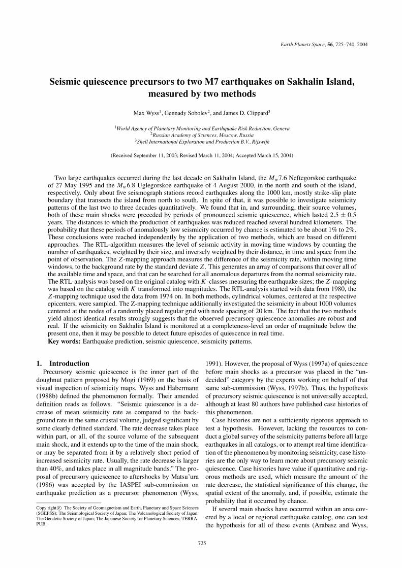
Fig. 1. Epicenter map of Sakhalin Island for 1974–1995.4 and M ≥ 3.4.The solid straight line marks the 1995 aftershock zone. The rectangleshows one of the definitions of the area of precursory quiescence.

1996b). However, often, there is only one large event avail-able for analysis (e.g. Wyss et al., 1997; Wyss and Marty-rosian, 1998). On Sakhalin Island, two main shocks of M7class occurred during the period for which modern seismicitydata are available; the Mw7.6 (Ms7.6) Neftegorskoe earth-quake of May 27, 1995, and the Mw6.8 (Ms7.1) Uglegorskoeearthquake of Aug. 4, 2000. Here, we examine the hypothe-sis that both of these large ruptures were preceded by seismic

quiescence in and near their source volumes.There exist different approaches to measure, map and

evaluate possible episodes of seismic quiescence. This hasthe disadvantage that the results reported by different authorsmay not be easily compared, but it has the advantage that onemay gain more confidence in a pattern that is detected bydifferent methods. Also, the uncertainties in the results maybe estimated by comparison and additional insights may begained because of intrinsic differences in the statistical char-acterization of anomalies. In the following, we present theanalysis of seismicity patterns in Sakhalin Island by two ap-proaches.

2. DataEarthquakes are produced at a relatively low rate all along

Sakhalin Island, which extends approximately 1000 km fromnorth to south (Fig. 1). Currently, there are about five seis-mograph stations monitoring this seismicity, with additionalreadings supplied from stations in Kamchatka and the Rus-sian mainland. The catalog for Sakhalin Island, of the Rus-sian Academy of Sciences (RAS), contains 2166 events withdepths less than 80 km for the period 1974–2002. About90% of the hypocenters in the catalog have depths H < 80km. In this depth-interval, 92% are shallower than 20 km.In the RAS catalog, the size of the earthquakes is mea-

sured by the energy class K , from which the magnitude,ML H , can be calculated by

ML H = (K − 1.2)/2 (1)

for events with depth H < 80 km (Soloviev and Solovieva,1967). The analysis using the RTL-algorithm was performedbased on the K -classification. In the Z -value method, mag-nitudes were used. The approach of dealing with the het-erogeneity of reporting, which is present in all catalogs, wasalso different in the two methods of analysis.Aftershocks add noise to both methods of seismicity rate

analysis used here. Therefore, we used declustered catalogsas the basic data sets. For the RTL-analysis, we eliminatedaftershocks using the program written by Smirnov (1998) onthe basis of the algorithm of Molchan and Dmitrieva (1991).In this approach, the principle of separating aftershocks fromother events, which are called background, is based on thecomparison of their functions and their distribution in timeand space. Background events are assumed to be uniformlydistributed in space and time. Aftershocks are assumed tobe normally (Gaussian) distributed in space and temporallygoverned by the Omori law. For the Z -value analysis, thealgorithm by Reasenberg (1985) was used for declustering.This method eliminates aftershocks, as well as clusters ofevents judged sufficiently close to each other in space andtime to be considered interdependent. With this algorithm,only 10% of the events are judged to be clusters, exclud-ing the aftershock sequence to the 1995 main shock. TheZ -analysis was done with both the raw and declustered cata-logs, and the differences in results are insignificant.The minimum magnitude of complete reporting (Mc and

the corresponding Kc) is defined as the magnitude to whichthe Gutenberg-Richter frequency-magnitude power law isvalid. Changes of this parameter with time are of concernto all investigations of seismicity rate. For this reason, we

M. WYSS AND J. D. CLIPPARD: SEISMIC QUIESCENCE PRECURSOR ON SAKHALIN 727

investigated the level and the stability of Kc and Mc. Forthe data set using K as measure of the earthquake size, itwas found that Kc = 8, using the algorithm developed bySmirnov (1998). This method is based on verification of thehypothesis that the observed size distribution agrees with theGutenberg-Richter relation. For the Z -value study the sameprinciple was used, but the catalog with M as the measure ofsize was searched for changes of Mc as a function of time,using the software package ZMAP (Wiemer, 2001). Thisanalysis showed that Mc was stable from 1974 on. For mostyears Mc = 3.4, especially in the 1970s and early 1980s.Mc = 3.4 corresponds to Kc = 8, according to (1).The reporting rate in the catalog was approximately con-

stant over long periods, but two instances of significantchange can be seen in cumulative plots of earthquakes asa function of time. These occurred in 1980 and in 1988.We investigated them by the algorithmGENAS (Habermann,1983) to determine if they showed features of artificial re-porting rate changes, such as are observed due to inadver-tent changes in magnitude scale. The magnitude signatures(Habermann, 1987) of both rate changes did not show fea-tures that could have been interpreted as magnitude shifts.We therefore accepted the catalog from 1974 on withoutchanges in the Z -value analysis. For the analysis with theRTL-algorithm, a different decision was made. Although itwas also found that the catalog was approximately completeat the Kc = 8 level back to 1974, the RTL-analysis was sen-sitive to the reporting change in 1980. It turned out that be-fore this time there were no K -values given between 8.5 and9, but afterwards all decimal K -values were present. There-fore, 1980 was selected as the starting date for data used inthe RTL-analysis.We consequently performed our analysis on several data

sets. (1) The declustered catalog with M ≥ Mc for the pe-riod 1974–1995.4, N = 401 events (Fig. 1). (2) All eventsreported in the catalog for the period 1974–1995.4, assum-ing that the percentage of incompletely recorded events re-mained the same through time. The number of events in thiscatalog were Nall = 529. (3) The catalog with aftershocksremoved and with K ≥ 8 for the period 1980–1995.4, forwhich N (K8) = 283.

In the end, the results of the two methods, using somewhatdifferent criteria to select the data, agree. This shows thatthe details of the data selection do not produce the observedanomalies.

3. Sakhalin Tectonics and Main Shock Source Pa-rameters

The seismic activity in Sakhalin Island is due to a stillpoorly understood plate boundary (Chapman and Solomon,1976; Seno et al., 1996). A near-vertical strike-slip faultzone, striking essentially NS, passes through the entire is-land, separating the Asian plate from the Okhotsk plate(Zanyukov, 1971). The seismicity is low and large fault rup-tures occur relatively infrequently.On May 27, 1995, an Mw7.6 earthquake devastated the

city of Neftegorsk in northern Sakhalin (Arefiev et al., 2000).This was one of the worst earthquake disasters in Russianhistory because 2800 people perished in the city of Nefte-gorsk. The length of the aftershock area was about 60 km,

and the rupture length of the main shock, estimated from sur-face wave analysis, was 20–30 km (Katsumata et al., 2002).A surface rupture of 35 km length and 7 m maximum dis-placement was mapped (Shimamoto et al., 1996). The rup-ture occurred along the previously mapped Gyrgylan’i-Ossoifault (Fournier et al., 1994). The extent of the aftershockzone according to Katsumata et al. (2002) is shown as a solidline in Fig. 1.

4. Methods4.1 The Z -value methodIn the Z -value method, we compare the mean seismicity

rate during a limited period and in a given area to the over-all average rate in that area. The intent is to detect possi-ble periods of anomalously low seismicity just before mainshocks near their epicenters, and to evaluate the statisticalsignificance of such a quiescence compared with all otherrate decreases that may have happened at random times andlocations. To achieve this, we rely on the standard deviate,Z , to estimate the significance of the rate change,

Z = (M1 − M2)/(S1/n1 + S2/n2)1/2 (2)

where M is the mean rate, S the variance and n the numberof events in the first and second period to be compared. Thelarger the Z -value, the more significant the observed differ-ence. Large numbers of samples enhance, large variancesin the samples diminish, the significance. This parametricstatistical method is based on the assumption of normallydistributed samples, but is approximately valid for other dis-tributions when the sample size is large.Samples for which the rate is to be compared with the

background rate are selected as follows. At every node ofa grid with spacing 20 km that covers the study area, thenearest N events are selected (N = 100, 150, 200 in differentruns). In each sample of N events, the rate inside a windowof Tw is compared to the rate in the rest of that sample (Tw =1.5, 2, 2.5 years). The window is placed at every possibleposition in time, from the beginning to the end, stepping byone month. A total of 256 Z -values are therefore calculatedfor the period 1974–1995.4 at each of the approximately1000 nodes. The set of Z -values thus generated for eachnode is defined as the ‘lta-function’ because the rate withinthe window is compared to the Long Term Average rate. Itcan be plotted as a function of time, at any given node, forvisual assessment of statistical significance of a rate change.Usually, we generate a Z -map from these results, defin-

ing the areas of exceptionally anomalous rates (e.g. Wiemerand Wyss, 1994), given the position of Tw just before themain shock, and at any other time of interest. In the caseof the Neftegorskoe earthquake, the density of earthquakesis so low that the samples overlap substantially. As a conse-quence, it makes no sense to plot a map. Nevertheless, thearray of about 2.6·105 Z -values generated is useful to answerthe question: Did at any time, and at any position in space anepisode of quiescence occur, similar to the one we propose asprecursor? If the answer is “no, not at similar significance,”then we claim that the quiescence hypothesis is tenable.Another common sense approach to define the volume of

possible precursory quiescence, is to sample the source vol-ume with a geometrically simple shape (circle or rectangle)


and to compare the rate in the last Tw with the previous back-ground rate in this sample. If quiescence is seen in such asample, then the size of the circle or rectangle is increased,until the significance of the quiescence, as measured by theZ -value, diminishes. This approach is based on the hypoth-esis that the quiescence is tied to the source volume and itssurroundings.To reduce subjectivity in the sampling to a minimum,

we use simple geometrical shapes and window steps in 0.5years, only. The position of the grid, which forms the cen-ter points of circular areas in which we search for anomaliesthat may exist in random locations and times, is chosen atrandom. The statistical significance of the observed maxi-mal Z -value are finally estimated by generating large num-bers of data sets with the same properties as the one at hand,and by computing a distribution of maximum Z -values forthe random data sets.4.2 The RTL-algorithmThe RTL-method uses three functions to measure the

state of seismicity at a given location as a function of time.R(x, y, z, t) assigns a decreasing weight to each earthquakein the catalog as a function of epicentral distance from thepoint of interest, T (x, y, z, t) decreases the weight of eachevent as a function of the difference from the time of interest,and L(x, y, z, t) weighs the contribution to the algorithm bythe rupture length of each event (Huang et al., 2002, 2001;Sobolev, 2001; Sobolev and Tyupkin, 1997, 1999).These functions are defined as

R(x, y, z, t) = [� exp(−ri/ro)] − Rltr

T (x, y, z, t) = [� exp(−(t − ti )/to)] − Tltr (3)

L(x, y, z, t) = [�(li/ri )p] − Lltr .

In these formulas, x , y, z, and t are the coordinates, thedepth and the analysis time, respectively. ri is the epicentraldistance from the location selected for analyses, ti is the oc-currence time of the past seismic events, and li is the lengthof rupture. The Rltr , Tltr , Lltr are the long-term averagesof these functions. By subtracting them, they eliminate thelinear trends of the corresponding functions. ro is a coef-ficient that characterizes the diminishing influence of moredistant seismic events; to is the coefficient characterizing therate at which the preceding seismic events are “forgotten”as the time of analysis moves on; and p is the coefficientthat characterizes the contribution of size of each precedingevent. With p = 1, 2 or 3, this quantity is proportional tosource length, square of rupture, or the energy, respectively.

R, T and L are dimensionless functions. They are fur-ther normalized by their standard deviations, σR , σT , and σL ,respectively. The product of the above three functions is cal-culated as the RTL-parameter, which describes the deviationfrom the background level of seismicity and is in units of thestandard deviation, σ = σRσT σL .

RT L = R(x, y, z, t)T (x, y, z, t)L(x, y, z, t). (4)

Various combinations of the R, T and L functions havebeen tested when evaluating the algorithm RTL. The fluctu-ations of their product have been found to be highly sensi-tive to quiescence anomalies and to be characterized by lowbackground noise.

A decrease of RTL means a decrease of seismicity com-pared to the background rate around the investigated place (aseismic quiescence). A recovery stage from the quiescenceto the background level can be considered as foreshock ac-tivation (in a broad sense). The RTL-method evaluates boththe seismic quiescence and the following stage of activation.In addition, the location of the maximum expression of ananomaly can be found by performing the RTL-calculationswith the centers of the sampling circles at the nodes of a grid.The original catalog for Sakhalin, prepared by the Geo-

physical Service of the RAS, contains the events character-ized by energy class K = log E , where E is the seismicenergy of the events in J . The length of rupture, li , in the L-function was calculated by the formula (Riznichenko, 1976).

Log l (km) = 0.244 log K − 2.266. (5)

5. Quiescence Measured by Z-values5.1 The Neftegorskoe Mw7.6 earthquake of May 27,

1995The cumulative numbers of earthquakes as a function of

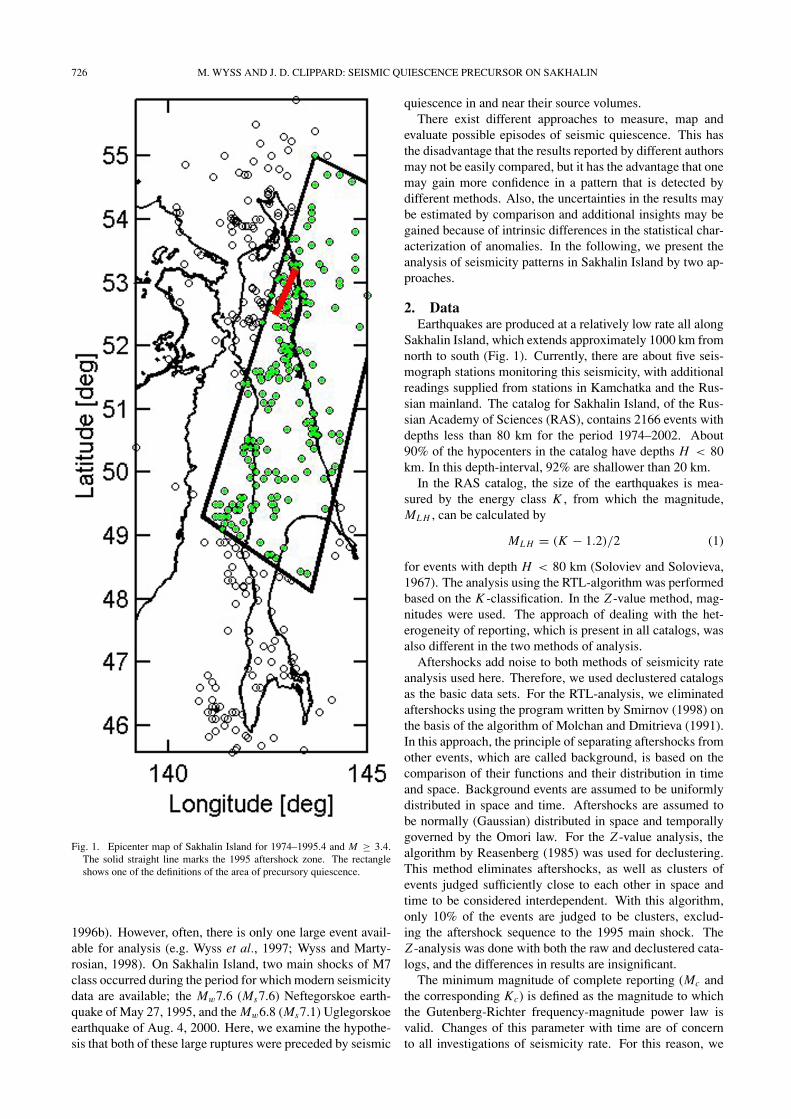
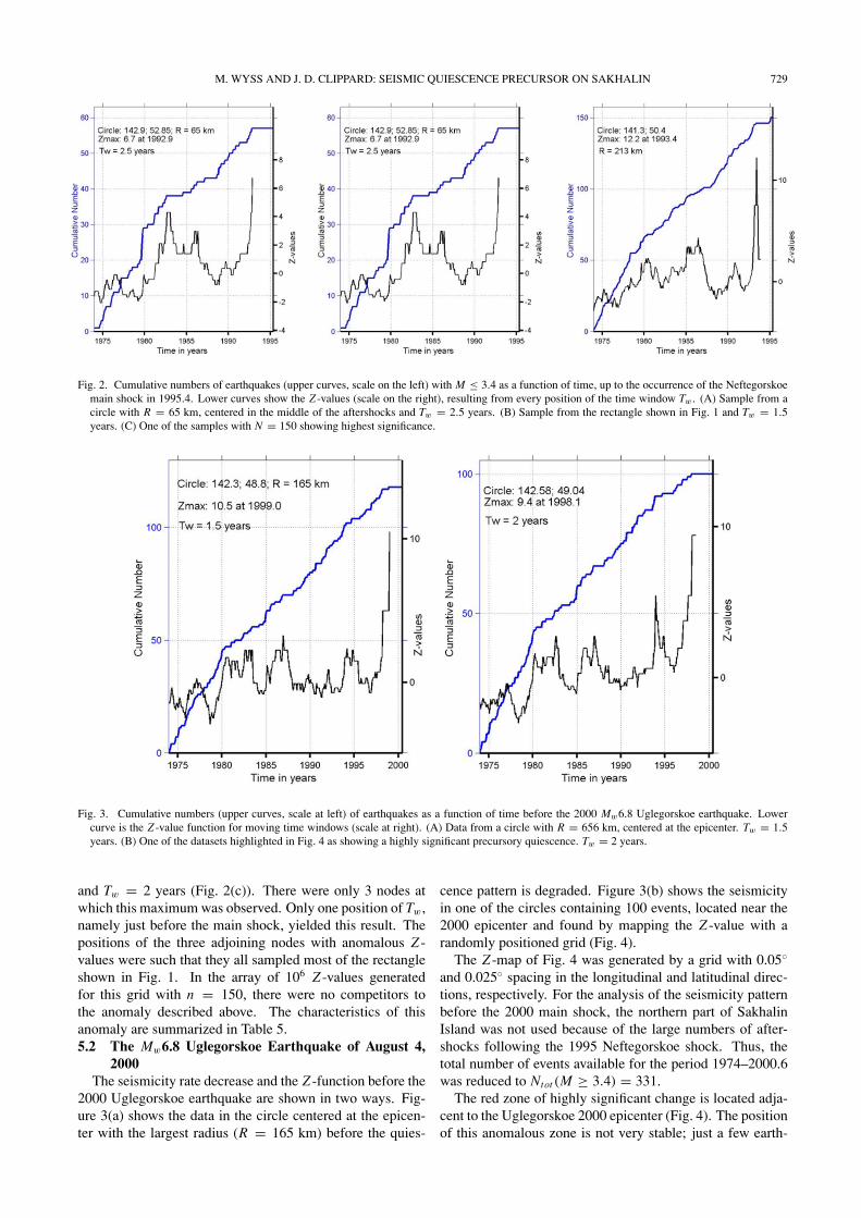
time for a circle with R = 65 km centered in the middle ofthe 1995 aftershock area (52.85◦N/142.9◦E), as mapped byKatsumata et al. (2002) shows an anomaly of no earthquakesduring the 2.7 years before the main shock (Fig. 2(a)). Dur-ing the first 18.7 years, 57 earthquakes occurred, which av-erages to a rate of 3 events/year. Thus, during the 2.7 yearspreceding the Neftegorskoe shock, nine events are expected,but none was recorded. If the radius is increased beyond 65km, a couple of earthquakes are picked up during the lasttwo years, and the pattern of quiescence is degraded. WithTw = 2.5 years and R = 65 km, the comparison of theseismicity rate during the last two years with the backgroundrate results in Z = 6.7. In this approach to identify the quies-cence, we simply increased the radius of a circle around thecenter of the aftershock activity until the anomalous patternwas degraded.In a second approach, we selected earthquakes inside a

rectangle with two sides parallel to the Neftegorskoe rupture.For small dimensions of this rectangle, the sample was ap-proximately the same as that selected by the circle and seenin Fig. 2(a). We then moved each side of the rectangle asfar away from the epicenter as we could without degradingthe pattern of precursory seismic quiescence. In this way,one finds that to the south, east and north the boundary canbe moved quite far (rectangle in Fig. 1), without degradingthe quiescence pattern (Fig. 2(b)). A single earthquake ispicked up near 52N/143E during the last two years beforethe main shock. Toward the west, however, some earth-quakes are picked up for this period from the cluster near52.3N/142E, degrading the pattern substantially. Hence wefind the limits of the rectangle as shown in Fig. 1.In this rectangle, with dimensions of 600 by 200 km,

210 earthquakes were recorded during the first 17.7 years,on average 12 events/year. During the last 1.8 years, oneearthquake was observed, instead of the 21 expected ones.With Tw = 1.5 years, the comparison of the rate during theanomalous time to the background leads to Z = 10.0.

Using the gridding approach, placing the grid at random,a maximum value of Z = 12.1 was found for N = 150


Fig. 2. Cumulative numbers of earthquakes (upper curves, scale on the left) with M ≤ 3.4 as a function of time, up to the occurrence of the Neftegorskoemain shock in 1995.4. Lower curves show the Z -values (scale on the right), resulting from every position of the time window Tw . (A) Sample from acircle with R = 65 km, centered in the middle of the aftershocks and Tw = 2.5 years. (B) Sample from the rectangle shown in Fig. 1 and Tw = 1.5years. (C) One of the samples with N = 150 showing highest significance.

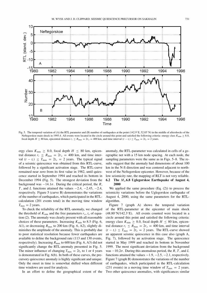
Fig. 3. Cumulative numbers (upper curves, scale at left) of earthquakes as a function of time before the 2000 Mw6.8 Uglegorskoe earthquake. Lowercurve is the Z -value function for moving time windows (scale at right). (A) Data from a circle with R = 656 km, centered at the epicenter. Tw = 1.5years. (B) One of the datasets highlighted in Fig. 4 as showing a highly significant precursory quiescence. Tw = 2 years.

and Tw = 2 years (Fig. 2(c)). There were only 3 nodes atwhich this maximumwas observed. Only one position of Tw,namely just before the main shock, yielded this result. Thepositions of the three adjoining nodes with anomalous Z -values were such that they all sampled most of the rectangleshown in Fig. 1. In the array of 106 Z -values generatedfor this grid with n = 150, there were no competitors tothe anomaly described above. The characteristics of thisanomaly are summarized in Table 5.5.2 The Mw6.8 Uglegorskoe Earthquake of August 4,

2000The seismicity rate decrease and the Z -function before the

2000 Uglegorskoe earthquake are shown in two ways. Fig-ure 3(a) shows the data in the circle centered at the epicen-ter with the largest radius (R = 165 km) before the quies-

cence pattern is degraded. Figure 3(b) shows the seismicityin one of the circles containing 100 events, located near the2000 epicenter and found by mapping the Z -value with arandomly positioned grid (Fig. 4).The Z -map of Fig. 4 was generated by a grid with 0.05◦

and 0.025◦ spacing in the longitudinal and latitudinal direc-tions, respectively. For the analysis of the seismicity patternbefore the 2000 main shock, the northern part of SakhalinIsland was not used because of the large numbers of after-shocks following the 1995 Neftegorskoe shock. Thus, thetotal number of events available for the period 1974–2000.6was reduced to Ntot (M ≥ 3.4) = 331.

The red zone of highly significant change is located adja-cent to the Uglegorskoe 2000 epicenter (Fig. 4). The positionof this anomalous zone is not very stable; just a few earth-


Fig. 4. Map of Z-values that result if the rate in the two years after 1998 is compared to the background rate before that time. For sampling, nodes werespaced 0.05 and 0.025 along the abscissa and ordinate respectively. At each node, the nearest 100 events were selected. Because of the low seismicity,the radii are typically 100 to 150 km, overlapping each other to a large extent. This means that the samples for the red area come from latitudes 47.5 to50.5, approximately. Dots mark epicenters. The star shows the epicenter of the 2000 Sakhalin main shock.

quakes can shift it by a few 10s of kilometers. This instabilityis due to the relatively low seismicity rate in all of Sakhalin.In such a case, the occurrence of a few events can degradethe significance of rate change.Both examples of cumulative seismicity curves show very

clear quiescence during the 1.5 to 2.5 years before the 2000main shock (Fig. 3). In the circle centered at the epicenter,117 events occurred during the first 25 years, yielding a meanrate of 4.9 events/year. Thus, 12 earthquakes are expectedduring the 2.5 years before the main shock, but only one was

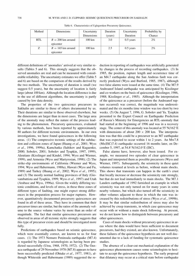
observed. The parameters of this anomaly are summarizedin Table 6.

6. Quiescence Measured by the RTL-Algorithm6.1 The Neftegorskoe Mw7.6 earthquake of May 27,

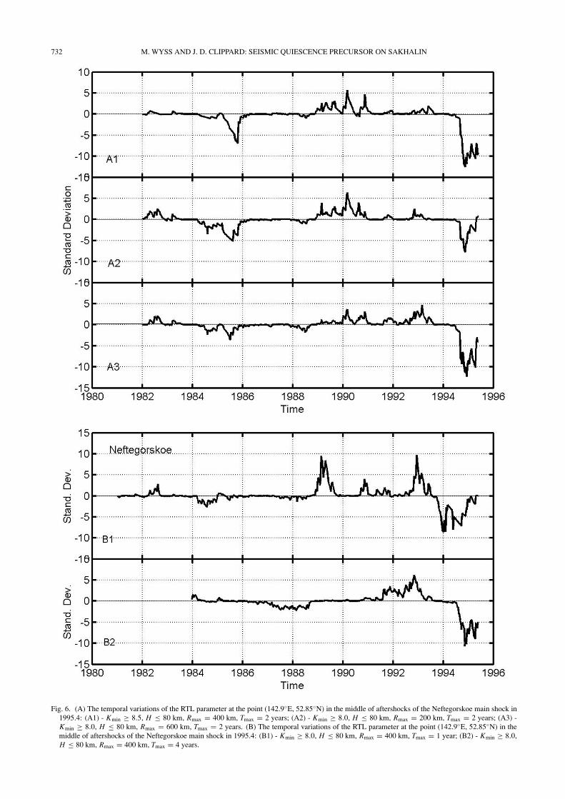
1995Figure 5 (curve A) shows the temporal variation

of the RTL-parameter at the center of the aftershocks(52.85◦N/142.9◦E). The events used were located in a cir-cle around this point and satisfied the following criteria: en-


Fig. 5. The temporal variation of (A) the RTL parameter and (B) number of earthquakes at the point (142.9◦E, 52.85◦N) in the middle of aftershocks of theNeftegorskoe main shock in 1995.4. All events were located in the circle around this point and satisfied the following criteria: energy class Kmin ≥ 8.0,focal depth H ≤ 80 km, epicentral distance ri ≤ Rmax = 2ro = 400 km, and time interval (t − ti ) ≤ Tmax = 2to = 2 years.

ergy class Kmin ≥ 8.0, focal depth H ≤ 80 km, epicen-tral distance ri ≤ Rmax = 2ro = 400 km, and time inter-val (t − ti ) ≤ Tmax = 2to = 2 years. The typical signalof a seismic quiescence was obtained from this RTL-curve,followed by a significant activation stage. The RTL-curveremained near zero from its first value in 1982, until quies-cence started in September 1994 and reached its bottom inDecember 1994 (Fig. 5). The strongest deviation from thebackground was −14.1σ . During the critical period, the R,T , and L functions attained the values −2.4, −2.45, −2.4,respectively. Figure 5 (curve B) demonstrates the variationsof the number of earthquakes, which participated in the RTL-calculation (201 events total) in the moving time windowTmax = 2 years.To check the reliability of the RTL-anomaly, we changed

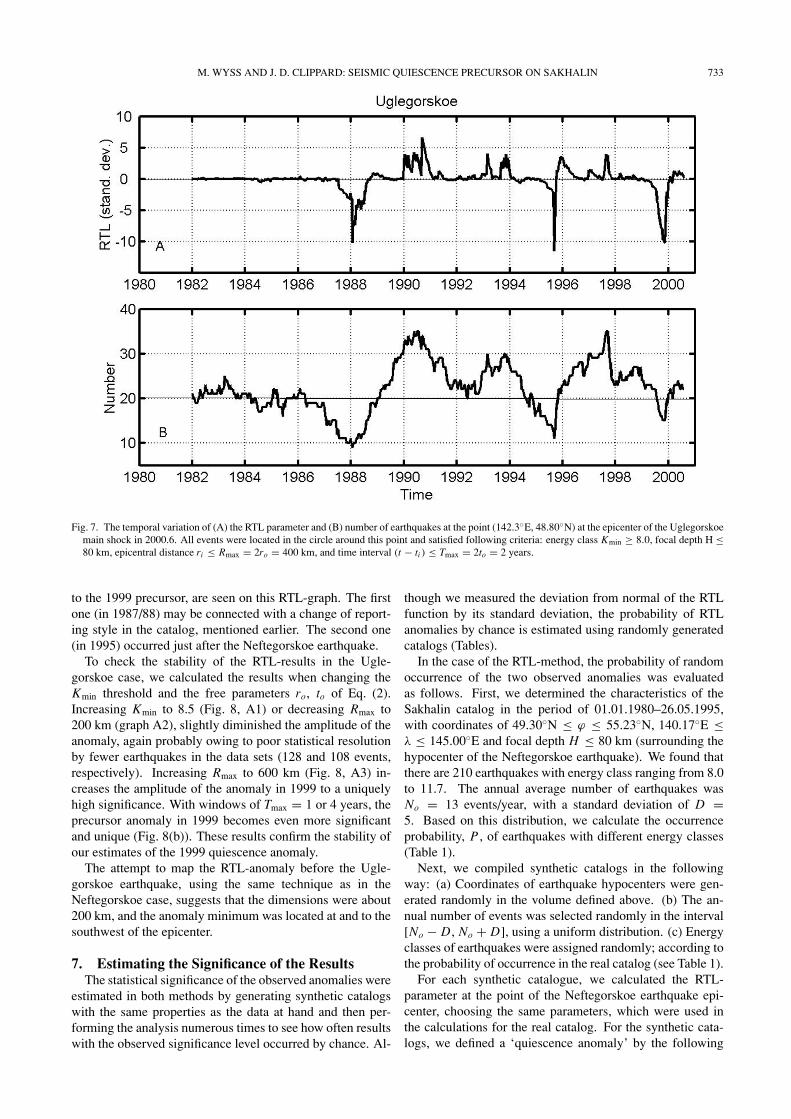
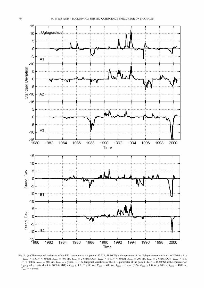
the threshold of Kmin and the free parameters ro, to of equa-tion (2). The anomaly was clearly present with all reasonablechoices of these parameters. Increasing Kmin to 8.5 (Fig. 6,A1), or decreasing Rmax to 200 km (Fig. 6, A2), slightly di-minishes the amplitude of the anomaly. This is probably dueto poor statistical resolution because fewer earthquakes areavailable to define the background rate (113 and 130 events,respectively). Increasing Rmax to 600 km (Fig. 6, A3) did notsignificantly change the RTL-anomaly presented in Fig. 5.The minor influence of changing Tmax = 2to to 1 or 4 yearsis demonstrated in Fig. 6(b). In both of these curves, the pre-cursory quiescence anomaly is highly significant and unique.Only the onset in time is somewhat shifted when differenttime windows are used for analysis.In an effort to define the geographical extent of the

anomaly, the RTL-parameter was calculated in cells of a ge-ographic net with a 15 km node spacing. At each node, thesampling parameters were the same as in Figs. 5–8. The re-sults suggest that the anomaly had dimensions of about 100km in the N-S direction and was centered adjacent to north-west of the Neftegorskoe epicenter. However, because of thelow seismicity rate, the mapping of RLT is not very reliable.6.2 The Mw6.8 Uglegorskoe Earthquake of August 4,

2000We applied the same procedure (Eq. (2)) to process the

seismicity variations before the Uglegorskoe earthquake ofAugust 4, 2000, using the same parameters for the RTL-algorithm.Figure 7 (graph A) shows the temporal variation

of the RTL-parameter at the epicenter of main shock(48.80◦N/142.3◦E). All events counted were located in acircle around this point and satisfied the following criteria:energy class Kmin ≥ 8.0, focal depth H ≤ 80 km, epicen-tral distance ri ≤ Rmax = 2ro = 400 km, and time interval(t − ti ) ≤ Tmax = 2to = 2 years. The RTL-curve showedan apparent seismic quiescence in this case also (graph A,Fig. 7), followed by an activation stage. The quiescencestarted in May 1999 and reached its bottom in November1999. The most significant deviation from the backgroundwas −10.2σ . During this anomalous period, the R, T , and Lfunctions attained the values −1.9, −2.5, −2.1, respectively.Figure 7 (graph B) demonstrates the variations of the numberof earthquakes, which participated in the RTL-calculation(231 events) in a moving time window of Tmax = 2 years.Two other quiescence anomalies, with significances similar


Fig. 6. (A) The temporal variations of the RTL parameter at the point (142.9◦E, 52.85◦N) in the middle of aftershocks of the Neftegorskoe main shock in1995.4: (A1) - Kmin ≥ 8.5, H ≤ 80 km, Rmax = 400 km, Tmax = 2 years; (A2) - Kmin ≥ 8.0, H ≤ 80 km, Rmax = 200 km, Tmax = 2 years; (A3) -Kmin ≥ 8.0, H ≤ 80 km, Rmax = 600 km, Tmax = 2 years. (B) The temporal variations of the RTL parameter at the point (142.9◦E, 52.85◦N) in themiddle of aftershocks of the Neftegorskoe main shock in 1995.4: (B1) - Kmin ≥ 8.0, H ≤ 80 km, Rmax = 400 km, Tmax = 1 year; (B2) - Kmin ≥ 8.0,H ≤ 80 km, Rmax = 400 km, Tmax = 4 years.


Fig. 7. The temporal variation of (A) the RTL parameter and (B) number of earthquakes at the point (142.3◦E, 48.80◦N) at the epicenter of the Uglegorskoemain shock in 2000.6. All events were located in the circle around this point and satisfied following criteria: energy class Kmin ≥ 8.0, focal depth H ≤80 km, epicentral distance ri ≤ Rmax = 2ro = 400 km, and time interval (t − ti ) ≤ Tmax = 2to = 2 years.

to the 1999 precursor, are seen on this RTL-graph. The firstone (in 1987/88) may be connected with a change of report-ing style in the catalog, mentioned earlier. The second one(in 1995) occurred just after the Neftegorskoe earthquake.To check the stability of the RTL-results in the Ugle-

gorskoe case, we calculated the results when changing theKmin threshold and the free parameters ro, to of Eq. (2).Increasing Kmin to 8.5 (Fig. 8, A1) or decreasing Rmax to200 km (graph A2), slightly diminished the amplitude of theanomaly, again probably owing to poor statistical resolutionby fewer earthquakes in the data sets (128 and 108 events,respectively). Increasing Rmax to 600 km (Fig. 8, A3) in-creases the amplitude of the anomaly in 1999 to a uniquelyhigh significance. With windows of Tmax = 1 or 4 years, theprecursor anomaly in 1999 becomes even more significantand unique (Fig. 8(b)). These results confirm the stability ofour estimates of the 1999 quiescence anomaly.The attempt to map the RTL-anomaly before the Ugle-

gorskoe earthquake, using the same technique as in theNeftegorskoe case, suggests that the dimensions were about200 km, and the anomaly minimum was located at and to thesouthwest of the epicenter.

7. Estimating the Significance of the ResultsThe statistical significance of the observed anomalies were

estimated in both methods by generating synthetic catalogswith the same properties as the data at hand and then per-forming the analysis numerous times to see how often resultswith the observed significance level occurred by chance. Al-

though we measured the deviation from normal of the RTLfunction by its standard deviation, the probability of RTLanomalies by chance is estimated using randomly generatedcatalogs (Tables).In the case of the RTL-method, the probability of random

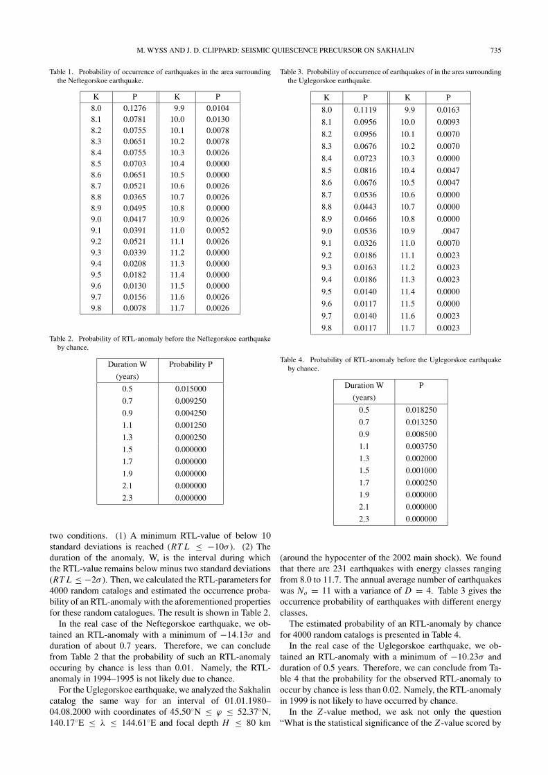
occurrence of the two observed anomalies was evaluatedas follows. First, we determined the characteristics of theSakhalin catalog in the period of 01.01.1980–26.05.1995,with coordinates of 49.30◦N ≤ ϕ ≤ 55.23◦N, 140.17◦E ≤λ ≤ 145.00◦E and focal depth H ≤ 80 km (surrounding thehypocenter of the Neftegorskoe earthquake). We found thatthere are 210 earthquakes with energy class ranging from 8.0to 11.7. The annual average number of earthquakes wasNo = 13 events/year, with a standard deviation of D =5. Based on this distribution, we calculate the occurrenceprobability, P , of earthquakes with different energy classes(Table 1).Next, we compiled synthetic catalogs in the following

way: (a) Coordinates of earthquake hypocenters were gen-erated randomly in the volume defined above. (b) The an-nual number of events was selected randomly in the interval[No − D, No + D], using a uniform distribution. (c) Energyclasses of earthquakes were assigned randomly; according tothe probability of occurrence in the real catalog (see Table 1).For each synthetic catalogue, we calculated the RTL-

parameter at the point of the Neftegorskoe earthquake epi-center, choosing the same parameters, which were used inthe calculations for the real catalog. For the synthetic cata-logs, we defined a ‘quiescence anomaly’ by the following


Fig. 8. (A) The temporal variations of the RTL parameter at the point (142.3◦E, 48.80◦N) at the epicenter of the Uglegorskoe main shock in 2000.6: (A1)- Kmin ≥ 8.5, H ≤ 80 km, Rmax = 400 km, Tmax = 2 years; (A2) - Kmin ≥ 8.0, H ≤ 80 km, Rmax = 200 km, Tmax = 2 years; (A3) - Kmin ≥ 8.0,H ≤ 80 km, Rmax = 600 km, Tmax = 2 years. (B) The temporal variations of the RTL parameter at the point (142.3◦E, 48.80◦N) at the epicenter ofUglegorskoe main shock in 2000.6: (B1) - Kmin ≥ 8.0, H ≤ 80 km, Rmax = 400 km, Tmax = 1 year; (B2) - Kmin ≥ 8.0, H ≤ 80 km, Rmax = 400 km,Tmax = 4 years.


Table 1. Probability of occurrence of earthquakes in the area surroundingthe Neftegorskoe earthquake.

K P K P8.0 0.1276 9.9 0.01048.1 0.0781 10.0 0.01308.2 0.0755 10.1 0.00788.3 0.0651 10.2 0.00788.4 0.0755 10.3 0.00268.5 0.0703 10.4 0.00008.6 0.0651 10.5 0.00008.7 0.0521 10.6 0.00268.8 0.0365 10.7 0.00268.9 0.0495 10.8 0.00009.0 0.0417 10.9 0.00269.1 0.0391 11.0 0.00529.2 0.0521 11.1 0.00269.3 0.0339 11.2 0.00009.4 0.0208 11.3 0.00009.5 0.0182 11.4 0.00009.6 0.0130 11.5 0.00009.7 0.0156 11.6 0.00269.8 0.0078 11.7 0.0026

Table 2. Probability of RTL-anomaly before the Neftegorskoe earthquakeby chance.

Duration W Probability P

(years)

0.5 0.015000

0.7 0.009250

0.9 0.004250

1.1 0.001250

1.3 0.000250

1.5 0.000000

1.7 0.000000

1.9 0.000000

2.1 0.000000

2.3 0.000000

two conditions. (1) A minimum RTL-value of below 10standard deviations is reached (RT L ≤ −10σ ). (2) Theduration of the anomaly, W, is the interval during whichthe RTL-value remains below minus two standard deviations(RT L ≤ −2σ ). Then, we calculated the RTL-parameters for4000 random catalogs and estimated the occurrence proba-bility of an RTL-anomaly with the aforementioned propertiesfor these random catalogues. The result is shown in Table 2.In the real case of the Neftegorskoe earthquake, we ob-

tained an RTL-anomaly with a minimum of −14.13σ andduration of about 0.7 years. Therefore, we can concludefrom Table 2 that the probability of such an RTL-anomalyoccuring by chance is less than 0.01. Namely, the RTL-anomaly in 1994–1995 is not likely due to chance.For the Uglegorskoe earthquake, we analyzed the Sakhalin

catalog the same way for an interval of 01.01.1980–04.08.2000 with coordinates of 45.50◦N ≤ ϕ ≤ 52.37◦N,140.17◦E ≤ λ ≤ 144.61◦E and focal depth H ≤ 80 km

Table 3. Probability of occurrence of earthquakes of in the area surroundingthe Uglegorskoe earthquake.

K P K P

8.0 0.1119 9.9 0.0163

8.1 0.0956 10.0 0.0093

8.2 0.0956 10.1 0.0070

8.3 0.0676 10.2 0.0070

8.4 0.0723 10.3 0.0000

8.5 0.0816 10.4 0.0047

8.6 0.0676 10.5 0.0047

8.7 0.0536 10.6 0.0000

8.8 0.0443 10.7 0.0000

8.9 0.0466 10.8 0.0000

9.0 0.0536 10.9 .0047

9.1 0.0326 11.0 0.0070

9.2 0.0186 11.1 0.0023

9.3 0.0163 11.2 0.0023

9.4 0.0186 11.3 0.0023

9.5 0.0140 11.4 0.0000

9.6 0.0117 11.5 0.0000

9.7 0.0140 11.6 0.0023

9.8 0.0117 11.7 0.0023

Table 4. Probability of RTL-anomaly before the Uglegorskoe earthquakeby chance.

Duration W P

(years)

0.5 0.018250

0.7 0.013250

0.9 0.008500

1.1 0.003750

1.3 0.002000

1.5 0.001000

1.7 0.000250

1.9 0.000000

2.1 0.000000

2.3 0.000000

(around the hypocenter of the 2002 main shock). We foundthat there are 231 earthquakes with energy classes rangingfrom 8.0 to 11.7. The annual average number of earthquakeswas No = 11 with a variance of D = 4. Table 3 gives theoccurrence probability of earthquakes with different energyclasses.The estimated probability of an RTL-anomaly by chance

for 4000 random catalogs is presented in Table 4.In the real case of the Uglegorskoe earthquake, we ob-

tained an RTL-anomaly with a minimum of −10.23σ andduration of 0.5 years. Therefore, we can conclude from Ta-ble 4 that the probability for the observed RTL-anomaly tooccur by chance is less than 0.02. Namely, the RTL-anomalyin 1999 is not likely to have occurred by chance.In the Z -value method, we ask not only the question

“What is the statistical significance of the Z -value scored by


Fig. 9. Alarm cube with Tw = 2 years and N = 100 events at each node, inwhich the time at each node is marked (circle), if Z ≤ 9.4. The durationof the time window is indicated by a vertical bar. In this 3-D presentation,the two horizontal axes are the latitude and longitude, the vertical axisshows time. For this Z -level, only one alarm-group is seen, located nearthe 2000 main shock epicenter and during the period just before it. Therest of the volume of time and space does not show a single anomaly,although more than 105 Z -value estimates exist.

the proposed precursor anomaly?” but also ”How often doesa similarly significant quiescence happen without a mainshock following it?” This second question addresses the pos-sibility that transients in the Earth may cause instances ofquiescence without following main shocks. To answer thefirst question, we also generate synthetic catalogs and simu-late the experiment many times, using the same parametersas in the real catalog. The only difference to the RTL-methodis that we do not pay attention to the magnitude distributionin the catalog, because this parameter is not used in the Z -map approach. To answer the second question, we searchthe results from the real catalog for episodes of highly sig-nificant quiescence at locations and times that are not relatedto main shocks. This is easily possible because we generatedan array of Z -values that compare the rate within all 2-yearwindows, and at every possible position in time, to the back-ground rate, at about 1000 locations.For the probability that the two anomalies are observed

by chance, the routines programmed in ZMAP version 5(Wiemer, 2001) also calculate values between 1% and 2%.For a graphical presentation of the answer to the secondquestion, ZMAP generates an alarm cube image (Fig. 9).For this 3-D presentation, one selects an ‘alarm-level,’ theZ -value above which one wishes to see the position in spaceand times of all occurrences. For both Sakhalin main shocks,

the alarm cubes show only the anomaly just before the re-spective main shocks (e.g. Fig. 9), if the alarm level is sethigh. This means that in both cases no alarms exist that rivalthe precursory alarm in statistical significance.

8. DiscussionThe data quality is satisfactory from the point of view of

homogeneous reporting. We detected a change in the re-porting procedure at the beginning of 1980 that disturbedthe RTL-algorithm and reduced the significance of the Z -value analysis. This was caused by the change to reportingall decimal K -classes after 1980.0, whereas before classeswere given in bins of 0.5 units only. Another change of re-porting appears to have happened in 1988.0, affecting mainlythe southern part of Sakhalin Island. The cause of this appar-ent change is not known.Visual inspection of the two quiescence anomalies is sub-

jectively striking. The cumulative number plots in Figs. 2and 3 climb at an approximately steady rate until the seis-micity stops completely during the last 2.5 years. Quantita-tive measurements of the significance and the uniqueness ofthese observations are necessary, however, to establish themas significant anomalies. The first step toward establishingthe statistical significance is the calculation of the parameterslta (Figs. 2 and 3) and RTL (Figs. 5, 6, 7 and 8) by the twomethods employed here, respectively. These curves showthat the quiescence anomalies in 1994 in the north and in1999 in the south are very clearly defined by the algorithms.The statistical significance of the two seismic quiescence

anomalies in northern and southern Sakhalin is finally es-tablished at the 98% to 99% confidence level by calculatingthe probability that they may occur by chance in data setsartificially generated and modeled on the real data set (Ta-bles 2 and 4). Some of the assumptions made for estimat-ing these significance levels are approximations. This meansthat the exact level of significance could be challenged onthe grounds that different assumptions should be used. Nev-ertheless, it is clear that at the very high significances wecalculate, other reasonable assumptions will also lead to highsignificances. In addition, we investigate the uniqueness ofthe anomalies, below. If those anomalies have never hap-pened at any time and in any volume, then we make a genericargument that these excursions from the mean are not nor-mal. These two lines of reasoning together make a strongcase that the phenomenon of anomalous quiescence is real.The uniqueness of the anomalies is established by a search

in all of Sakhalin and during all of time (covered by the cat-alog) for periods of quiescence with similar statistical sig-nificance as the two anomalies discussed above. In the Z -map method, the search was performed using the grid with20 km node separation and moving the window by steps ofthree months. In the RTL-method, the node separation was100 km. Neither method detected any other anomaly withanywhere near the significance of that observed before theNeftegorskoe earthquake. For the Uglegorskoe anomaly, theRTL-method found one false alarm with a value of −10.5sigma (compared to the precursor anomaly in 2000 of −10.2sigma). This false RTL-alarm is seen in Figs. 7 and 8 in1987. The RTL-method detected no other anomalies withvalues less than −5 sigma. Using the Zmap method, the


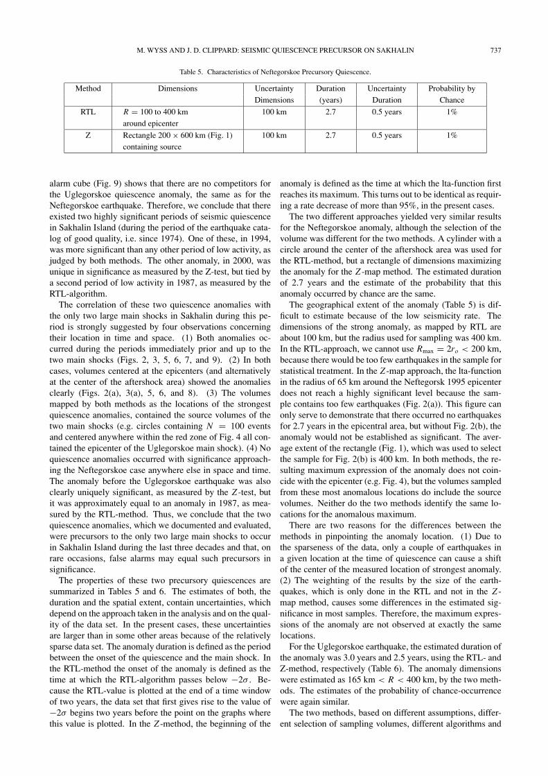
Table 5. Characteristics of Neftegorskoe Precursory Quiescence.

Method Dimensions Uncertainty Duration Uncertainty Probability byDimensions (years) Duration Chance

RTL R = 100 to 400 km 100 km 2.7 0.5 years 1%around epicenter

Z Rectangle 200 × 600 km (Fig. 1) 100 km 2.7 0.5 years 1%containing source

alarm cube (Fig. 9) shows that there are no competitors forthe Uglegorskoe quiescence anomaly, the same as for theNeftegorskoe earthquake. Therefore, we conclude that thereexisted two highly significant periods of seismic quiescencein Sakhalin Island (during the period of the earthquake cata-log of good quality, i.e. since 1974). One of these, in 1994,was more significant than any other period of low activity, asjudged by both methods. The other anomaly, in 2000, wasunique in significance as measured by the Z-test, but tied bya second period of low activity in 1987, as measured by theRTL-algorithm.The correlation of these two quiescence anomalies with

the only two large main shocks in Sakhalin during this pe-riod is strongly suggested by four observations concerningtheir location in time and space. (1) Both anomalies oc-curred during the periods immediately prior and up to thetwo main shocks (Figs. 2, 3, 5, 6, 7, and 9). (2) In bothcases, volumes centered at the epicenters (and alternativelyat the center of the aftershock area) showed the anomaliesclearly (Figs. 2(a), 3(a), 5, 6, and 8). (3) The volumesmapped by both methods as the locations of the strongestquiescence anomalies, contained the source volumes of thetwo main shocks (e.g. circles containing N = 100 eventsand centered anywhere within the red zone of Fig. 4 all con-tained the epicenter of the Uglegorskoe main shock). (4) Noquiescence anomalies occurred with significance approach-ing the Neftegorskoe case anywhere else in space and time.The anomaly before the Uglegorskoe earthquake was alsoclearly uniquely significant, as measured by the Z -test, butit was approximately equal to an anomaly in 1987, as mea-sured by the RTL-method. Thus, we conclude that the twoquiescence anomalies, which we documented and evaluated,were precursors to the only two large main shocks to occurin Sakhalin Island during the last three decades and that, onrare occasions, false alarms may equal such precursors insignificance.The properties of these two precursory quiescences are

summarized in Tables 5 and 6. The estimates of both, theduration and the spatial extent, contain uncertainties, whichdepend on the approach taken in the analysis and on the qual-ity of the data set. In the present cases, these uncertaintiesare larger than in some other areas because of the relativelysparse data set. The anomaly duration is defined as the periodbetween the onset of the quiescence and the main shock. Inthe RTL-method the onset of the anomaly is defined as thetime at which the RTL-algorithm passes below −2σ . Be-cause the RTL-value is plotted at the end of a time windowof two years, the data set that first gives rise to the value of−2σ begins two years before the point on the graphs wherethis value is plotted. In the Z -method, the beginning of the

anomaly is defined as the time at which the lta-function firstreaches its maximum. This turns out to be identical as requir-ing a rate decrease of more than 95%, in the present cases.The two different approaches yielded very similar results

for the Neftegorskoe anomaly, although the selection of thevolume was different for the two methods. A cylinder with acircle around the center of the aftershock area was used forthe RTL-method, but a rectangle of dimensions maximizingthe anomaly for the Z -map method. The estimated durationof 2.7 years and the estimate of the probability that thisanomaly occurred by chance are the same.The geographical extent of the anomaly (Table 5) is dif-

ficult to estimate because of the low seismicity rate. Thedimensions of the strong anomaly, as mapped by RTL areabout 100 km, but the radius used for sampling was 400 km.In the RTL-approach, we cannot use Rmax = 2ro < 200 km,because there would be too few earthquakes in the sample forstatistical treatment. In the Z -map approach, the lta-functionin the radius of 65 km around the Neftegorsk 1995 epicenterdoes not reach a highly significant level because the sam-ple contains too few earthquakes (Fig. 2(a)). This figure canonly serve to demonstrate that there occurred no earthquakesfor 2.7 years in the epicentral area, but without Fig. 2(b), theanomaly would not be established as significant. The aver-age extent of the rectangle (Fig. 1), which was used to selectthe sample for Fig. 2(b) is 400 km. In both methods, the re-sulting maximum expression of the anomaly does not coin-cide with the epicenter (e.g. Fig. 4), but the volumes sampledfrom these most anomalous locations do include the sourcevolumes. Neither do the two methods identify the same lo-cations for the anomalous maximum.There are two reasons for the differences between the

methods in pinpointing the anomaly location. (1) Due tothe sparseness of the data, only a couple of earthquakes ina given location at the time of quiescence can cause a shiftof the center of the measured location of strongest anomaly.(2) The weighting of the results by the size of the earth-quakes, which is only done in the RTL and not in the Z -map method, causes some differences in the estimated sig-nificance in most samples. Therefore, the maximum expres-sions of the anomaly are not observed at exactly the samelocations.For the Uglegorskoe earthquake, the estimated duration of

the anomaly was 3.0 years and 2.5 years, using the RTL- andZ-method, respectively (Table 6). The anomaly dimensionswere estimated as 165 km < R < 400 km, by the two meth-ods. The estimates of the probability of chance-occurrencewere again similar.The two methods, based on different assumptions, differ-

ent selection of sampling volumes, different algorithms and


Table 6. Characteristics of Uglegorskoe Precursory Quiescence.

Method Dimensions Uncertainty Duration Uncertainty Probability byDimensions (years) Duration Chance

RTL R = 200 km around 100 km 3.0 0.5 years 2%epicenter

Z R = 165 km around 100 km 2.5 0.5 years 2%epicenter

different definitions of ‘anomalies’ arrived at very similar re-sults (Tables 5 and 6). This strongly suggests that the ob-served anomalies are real and can be measured with consid-erable reliability. The uncertainty estimates we offer (Table 5and 6) are based on the comparison of the results derived bythe two methods. The uncertainty of duration is small (wesuggest 0.5 years), but the uncertainty of location is fairlylarge (about 100 km). Although the location difference is dueto the use of different algorithms, the uncertainty is partlycaused by low data density.The properties of the two quiescence precursors in

Sakhalin are similar to those of others documented by us.Their durations are similar to those observed elsewhere, butthe dimensions are larger than in most cases. The large areaof the anomaly may reflect the nature of the process lead-ing to the phenomenon. Precursory quiescences, evaluatedby various methods, have been reported by approximately80 authors for different tectonic environments. In our owninvestigations, we have found quiescences in the followingareas. (1) The compressive tectonic settings of the subduc-tion and collision zones of Japan (Huang et al., 2001; Wysset al., 1996, 1999a), Kamchatka (Saltikov and Kugaenko,2000; Sobolev, 2001; Sobolev and Tyupkin, 1997, 1999),Aleutians (Kisslinger and Kindel, 1994; Wyss and Wiemer,1999), and Armenia (Wyss and Martyrosian, 1998); (2) Thestrike-slip environments of California (Wiemer and Wyss,1994; Wyss and Habermann, 1988a), Hawaii (Wyss and Fu,1989) and Turkey (Huang et al., 2002; Wyss et al., 1995);and (3) The mostly normal faulting provinces of Italy (Gio-vambattista and Tyupkin, 1999; Wyss et al., 1997) and Utah(Arabasz and Wyss, 1996a). Given the widely differing tec-tonic conditions, and levels of stress, in these three zones ofdifferent types of faulting, one might expect strong differ-ences in the preparation process for major ruptures. How-ever, quantitatively documented precursory quiescences arefound in all of these areas. They have in common that theirprecursor times are similar, but the ratios of the anomaly vol-ume to the source volume varies by more than an order ofmagnitude. The fact that similar quiescence precursors areobserved in areas of all tectonic styles strongly suggests thatthis type of precursor exists and should be investigated morefully.Predictions of earthquakes based on seismic quiescence,

which were essentially correct, are known to us for fourcases. (1) The 1973 Nemuro Peninsula earthquake (M7.4)is regarded by Japanese seismologists as having been pre-dicted successfully (Utsu, 1968, 1970, 1972). (2) The Oax-aca earthquake of 29 November 1978 (M7.8) appears to havebeen successfully predicted (Ohtake et al., 1977, 1981), al-though Whiteside and Habermann (1989) suggested the re-

duction in reporting of earthquakes was artificially generatedby changes in the process of recording earthquakes. (3) In1985, the position, rupture length and occurrence time ofan M4.7 earthquake along the San Andreas fault was cor-rectly predicted (Wyss and Burford, 1985, 1987), althoughtwo false alarms were issued at the same time. (4) The M7.9Andreanof Island earthquake was anticipated by Kisslingerand co-workers on the basis of quiescence (Kisslinger, 1986,1988; Kisslinger et al., 1985). Although the interpretationof the quiescence as a precursor (before the Andreanof rup-ture occurred) was correct, the magnitude was underesti-mated and the six months time window was too short by twoweeks. (5) On August 7, 1996, G. Sobolev and Yu. Tyupkinpresented to the Expert Council on Earthquake Predictionof Russia’s Ministry for Emergencies an RTL-anomaly thathad started at the beginning of 1996 and was in a recoverystage. The center of this anomaly was located at 55◦N/162◦Ewith dimensions of about 200 × 200 km. The interpreta-tion was that this could be a precursor to an M7 earthquakethat was expected to occur within 1 to 2 years. An Mw7.8(Ms(ISC)7.4) earthquake occurred 16 months later, on De-cember 5, 1997, at 54.8◦N/162.0◦E (ISC).False alarms have, however, also been issued. For ex-

ample, we measured two episodes of clear quiescence inJapan and interpreted them as possible precursors (Wyss andWiemer, 1997). Subsequently, the seismicity in these quietvolumes resumed at levels as before, without main shocks.This shows that transients can happen in the earth’s crustthat locally increase or decrease the seismicity rate strongly,but that do not lead immediately to main shocks. The M7.1Landers earthquake of 1992 furnished an example in whichseismicity was not only turned on for many years in somenearby volumes, but which also turned off the seismicity inother volumes adjacent to those in which the rate was in-creased by this redistributions of stress (Wyss et al., 1999b).It may be that similar redistribution of stress may also beachieved by creep transients, in which case quiescence mayoccur with or without a main shock following. At present,we do not know how to distinguish between precursory andother quiescences.Cases of main shocks without precursory quiescence in ar-

eas where the data would have been sufficient to documentprecursors, had they existed, are also known. Unfortunately,these failures of the quiescence hypothesis are not well doc-umented due to a lack of funding for systematic quiescencestudies.The absence of a clear-cut mechanical explanation of the

quiescence phenomenon causes some seismologists to hesi-tate to accept the quiescence hypothesis. The early proposalthat dilatancy may occur at a critical state before earthquake


ruptures and cause hardening of source volumes (Scholz etal., 1973) has never been disproved, but it has gone out ofvogue. In the two Sakhalin cases analysed here, it is diffi-cult to imagine that dilatancy hardening could occur in vol-umes with dimensions of several hundred kilometers. Theidea that precursory creep might cause a redistribution (withlocal reduction) of stress, and hence quiescence, is also old(e.g. Sobolev, 1995; Stuart, 1979). It is also not easy to ac-cept the idea that strain softening might influence volumes atlarge distances. However, the evidence associated with somerecent earthquakes clearly shows that the seismicity budgetat large distances can be influenced strongly and over longperiods (e.g. Bodin et al., 1994; Gomberg and Davis, 1996;Harris and Simpson, 1992; Hill et al., 1993, 1995; Stein etal., 1992; Wyss and Wiemer, 2000). Correlation with mea-surements of other parameters, such as crustal deformations,could be helpful in formulating an authoritative model forthe phenomenon of precursory quiescence and for a betterunderstanding of the initiation process of major crustal fail-ure along faults better.Although we are far from believing that earthquake pre-

diction could soon become commonplace, it seems not un-reasonable to work toward achieving some successes in fa-vorable cases. Once Sakhalin has a new seismograph net-work, it would be possible to detect episodes of quies-cence as demonstrated here. However, it would not be easyto predict the location or magnitude of a possible futuremain shock. The location cannot be pinpointed because theanomalous volumes were large (half of Sakhalin Island). Toestimate the magnitude would also be difficult, because thefeatures of the two anomalies reported here are very similar,although the magnitudes of the main shocks are not (Mw6.8and Mw7.6). Nevertheless, we think it would be a mistakenot to try and gather experience with forecasting earthquakesbased on precursory seismic quiescence, a phenomenon thatsometimes produces clear signals.

Acknowledgments. We thank Sakhalin Energy Investment Co.(SEIC) for supporting this research. SEIC is the operator of theSakhalin II oil and gas venture, and is making significant upgradesto the island’s infrastructure, including the seismic monitoring net-work. We also thank the Russian Academy of Sciences for supply-ing the data, and S. Wiemer for his software ZMAP and advice forplotting.

ReferencesArabasz, W. T. and M. Wyss, Quiescence in Utah, EOS, 102, 9999, 1996a.Arabasz, W. T. and M. Wyss, Significant precursory seismic quiescences in

the extensional Wasatch front region Utah, EOS, 77, F455, 1996b.Arefiev, S., E. Rogozhin, R. Tatevossian, L. Rivera, and A. Cisternas, The

Neftegorsk (Sakhalin Island) 1995 earthquake: A rare interplate event,Geophys. J. Int., 143, 595–607, 2000.

Bodin, P., R. Bilham, J. Behr, J. Gomberg, and K. W. Hudnut, Slip triggeredon southern California faults by the 1992 Jushoa Tree, Landers and BigBear earthquakes, Bull. Seism. Soc. Am., 84, 806–816, 1994.

Chapman, M. E. and S. C. Solomon, North American-Eurasian plate bound-ary in northeast Asia, J. Geophys. Res., 81, 921–930, 1976.

Fournier, M., L. Jolivet, P. Huchon, K. F. Sergeyev, and L. S. Oscorbin,Neogene strike-slip faulting in Sakhalin and the Japan Sea opening, J.Geophys. Res., 99, 2701–2725, 1994.

Giovambattista, R. D. and Y. S. Tyupkin, The fine structure of the dynamicsof seismicity before m >= 4.5 earthquakes in the area of Reggio Emilia(Northern Italy), Annali di Geofisica, 42(5), 897–909, 1999.

Gomberg, J. and S. Davis, Stress/strain changes and triggered seismicityfollowing the Mw7.3 Landers, California, earthquake, J. Geophys. Res.,

101, 751–764, 1996.Habermann, R. E., Teleseismic detection in the Aleutian Island arc, J. Geo-

phys. Res., 88, 5056–5064, 1983.Habermann, R. E., Man-made changes of Seismicity rates, Bull. Seism. Soc.

Am., 77, 141–159, 1987.Harris, R. A. and R. W. Simpson, Changes in static stress on southern

California faults after the 1992 Landers earthquake, Nature, 360, 251–254, 1992.

Hill, D. P. et al., Seismicity remotely triggered by the magnitude 7.3 Lan-ders, California, earthquake, Science, 260, 1617–1623, 1993.

Hill, D. P., M. J. S. Josnston, and J. O. Langbein, Response of Long Valleycaldera to the Mw=7.3 Landers, California, earthquake, J. Geophys. Res.,100, 12985–13005, 1995.

Huang, Q., G. Sobolev, and T. Nagao, Characteristics of seismic quiescenceand activation patterns before the M = 7.2 Kobe earthquake, January 17,1995, Tectonophysics, 337, 99–116, 2001.

Huang, Q., A. O. Oncel, and G. A. Sobolev, Precursory seismicity changesassociated with the Mw=7.4 Izmit earthquake, August 17 1999, Geophys.J. Int., 151, 235–242, 2002.

Katsumata, K., M. Kasahara, M. Ichiyanagi, M. Kikuchi, R.-S. Sen, C.-U. Kim, A. Ivaschenko, and R. Tatevossian, The May 27, 1995 Ms =7.6 Northern Sakhalin earthquake: An earthquake on an uncertain plateboundary, Bull. Seism. Soc. Am., 94, 117–130, 2004.

Kisslinger, C., Seismicity patterns in the Adak seismic zone and the short-term outlook for a major earthquake, in Meeting of the National Earth-quake Prediction Evaluation Council, pp. 119–134, Anchorage, Alaska,1986.

Kisslinger, C., An experiment in earthquake prediction and the 7 May 1986Andreanof Islands earthquake, Bull. Seism. Soc. Am., 78, 218–229, 1988.

Kisslinger, C., C. McDonald, and J. R. Bowman, Precursory time-spacepatterns of seismicity and their relation to fault processes in the centralAleutian Islands seismic zone, in IASPEI, 23d general assembly, pp. 32,Tokyo, Japan, 1985.

Kisslinger, K. and B. Kindel, A comparison of seismicity rates near Adakisland, Alaska, September 1988 through May 1990 with rates before the1982 to 1986 apparent quiescence, Bull. Seism. Soc. Am., 84, 1560–1570,1994.

Matsu’ura, R. S., Precursory quiescence and recovery of aftershock activitybefore some large aftershocks, Bull. Earthq. Res. Inst., 61, 1–65, 1986.

Mogi, K., Some features of recent Seismic activity in and near Japan (2),Activity before and after great earthquakes, Bull. Earthq. Res. Inst., Univ.of Tokyo, 47, 395–417, 1969.

Molchan, G. M. and O. E. Dmitrieva, Identification of aftershocks: Reviewand new approaches, Computative Seismology, 24, 19–50, 1991 (in Rus-sian).

Ohtake, M., T. Matumoto, and G. V. Latham, Seismicity gap near Oaxaca,Southern Mexico, as a probable precursor to a large earthquake, Pageoph,115, 375–385, 1977.

Ohtake, M., T. Matumoto, and G. V. Latham, Evaluation of the forecastof the 1978 Oaxaca, Southern Mexico earthquake based on a precursorySeismic quiescence, in: Earthquake Prediction, Maurice Ewing Series,Amer. Geophys. Union, 4, 53–62, 1981.

Reasenberg, P. A., Second-order moment of Central California Seismicity,J. Geophys. Res., 90, 5479–5495, 1985.

Riznichenko, Y. V., Dimensions of the crustal earthquake focus and theseismic moment, Research in Earthquake Physics M., Nauka, 9–27, 1976(in Russian).

Saltikov, V. A. and Y. A. Kugaenko, Seismic quiescence before two strongearthqaukes 1996 on Kamchatka, Volkanologiya i Seismologiya, 1, 57–65, 2000.

Scholz, C. H., L. R. Sykes, and Y. P. Aggarwal, Earthquake prediction: aphysical basis, Science, 181, 803–810, 1973.

Seno, T., T. Sakurai, and S. Stein, Can the Okhotsk plate be discriminatedfrom the North American plate?, J. Geophys. Res., 101, 11305–11315,1996.

Shimamoto, T., M. Watanabe, Y. Suzuki, A. Kozhurin, M. Strel’tsov, andE. Rogozhin, Surface faults and damage associated with the 1995 Nefte-gorsk earthquake, J. Geol. Soc. Japan, 102, 894–907, 1996 (in Japanese).

Smirnov, V. B., Earthquake catalogs: Evaluation of data completeness,Volkanologiya i Seismologiya, 19, 433–446, 1998.

Sobolev, G., The examples of earthquake preparation in Kamchatka andJapan, Tectonophysics, 338, 269–279, 2001.

Sobolev, G. A., Fundamentals of Earthquake Prediction, 162 pp., Electro-magnetic Research Center, Moscow, 1995.

Sobolev, G. A. and Y. S. Tyupkin, Low-seismicity precursors of large earth-quakes in Kamchatka, Volcanology and Seismology, 18, 433–446, 1997.


Sobolev, G. A. and Y. S. Tyupkin, Precursory phases, seismicity precursors,and earthquake prediction in Kamchatka, Volkanologiya i Seismologiya,20, 615–627, 1999.

Soloviev, S. L. and O. N. Solovieva, The relation between the energy classand magnitude of Kuril earthquakes, Fizika Zemly, 2, 13–23, 1967 (inRussian).

Stein, R. S., G. C. P. King, and J. Lin, Change in failure stress on the SanAndreas and surrounding faults caused by the 1992 M = 7.4 Landersearthquake, Science, 258, 1328–1332, 1992.

Stuart, W. D., Strain softening prior to two-dimensional strike slip earth-quakes, J. Geophys. Res., 84, 1063–1070, 1979.

Utsu, T., Seismic activity in Hokkaido and its vicinity, Geophys. Bull.Hokkaido Univ., 20, 51–75, 1968 (in Japanese).

Utsu, T., Seismic activity and seismic observation in Hokkaido in recentyears, Report of the Coodinating Committee for Earthquake Prediction,2, 1–2, 1970 (in Japanese).

Utsu, T., Large earthquakes near Hokkaido and the expectancy of the oc-currence of a large earthquakes off Nemuro, Report of the CoodinatingCommitee for Earthquake Prediction, 7, 7–13, 1972 (in Japanese).

Whiteside, L. and R. E. Habermann, The seismic quiescence prior to the1978 Oaxaca, Mexico, earthquake is not a precursor to that earthquake,abstract, in IASPEI, 25th General Assembly, pp. 339, Istanbul, Turkey,1989.

Wiemer, S., A software package to analyze seismicity: ZMAP, Seismologi-cal Research Letters, 373–382, 2001.

Wiemer, S. and M. Wyss, Seismic quiescence before the Landers (M = 7.5)and Big Bear (M = 6.5) 1992 earthquakes, Bull. Seism. Soc. Am., 84,900–916, 1994.

Wyss, M., Evaluation of Proposed Earthquake Precursors, 94 pp., Wash-ington, 1991.

Wyss, M., Nomination of precursory seismic quiescence as a significantprecursor, Pure and Applied Geophysics, 149, 79–114, 1997a.

Wyss, M., Second round of evaluations of proposed earthquake precursors,Pure and Applied Geophysics, 149, 3–16, 1997b.

Wyss, M. and R. O. Burford, Current episodes of seismic quiescence alongthe San Andreas Fault between San Juan Bautista and Stone Canyon,California: Possible precursors to local moderate main shocks, U.S. Geol.Survey open-file report, 85-754, 367-426, 1985.

Wyss, M. and R. O. Burford, A predicted earthquake on the San Andreasfault, California, Nature, 329, 323–325, 1987.

Wyss, M. and Z. X. Fu, Precursory seismic quiescence before the January

1982 Hilea Hawaii earthquake, Bull. Seism. Soc. Am., 79, 756–773, 1989.Wyss, M. and R. E. Habermann, Precursory quiescence before the August

1982 Stone Canyon, San Andreas fault, earthquakes, Pure and AppliedGeophysics, 126, 333–356, 1988a.

Wyss, M. and R. E. Habermann, Precursory Seismic quiescence, Pure andApplied Geophysics, 126, 319–332, 1988b.

Wyss, M. and A. H. Martyrosian, Seismic quiescence before the M7, 1988,Spitak earthquake, Armenia, Geophysical Journal International, 124,329–340, 1998.

Wyss, M. and S. Wiemer, Two current seismic quiescences within 40 km ofTokyo, Geophysical Journal International, 128, 459–473, 1997.

Wyss, M. and S. Wiemer, How can one test the seismic gap hypothesis? TheCase of repeated ruptures in the Aleutians., Pure and Applied Geophysics,155, 259–278, 1999.

Wyss, M. and S. Wiemer, Change in the probability for earthquakes inSouthern California due to the Landers magnitude 7.3 earthquake, Sci-ence, 290, 1334–1338, 2000.

Wyss, M., M. Westerhaus, H. Berkhemer, and R. Ates, Precursory seismicquiescence in the Mudurnu Valley, North Anatolian fault zone, Turkey,Geophysical Journal International, 123, 117–124, 1995.

Wyss, M., K. Shimazaki, and T. Urabe, Quantitative mapping of a precur-sory quiescence to the Izu-Oshima 1990 (M6.5) earthquake, Japan, Geo-physical Journal International, 127, 735–743, 1996.

Wyss, M., R. Console, and M. Murru, Seismicity rate change before theIrpinia (M = 6.9) 1980 earthquake, Bull. Seism. Soc. Am., 87, 318–326,1997.

Wyss, M., A. Hasegawa, S. Wiemer, and N. Umino, Quantitative mappingof precursory seismic quiescence before the 1989, M7.1, off-Sanrikuearthquake, Japan, Annali di Geophysica, 42, 851–869, 1999a.

Wyss, M., S. Hreinsdottir, and D. A. Marriott, Southern extent of the Oc-tober 1999 M7.1 Hector Mine earthquake limited by Coulomb stresschanges due to the M7.3 Landers earthquake of 1992, EOS, abstract,1999b (in press).

Zanyukov, V. N., The central Sakhalin fault and its role in the tectonicevolution of the island, Dokl. Akad. Nauk SSSR, Engl. Transl., 196, 85,1971.

M. Wyss (e-mail: [email protected]), G. Sobolev, and J. D. Clip-pard

Documents

Seismic quiescence precursors to two M7 earthquakes on ... · PDF fileSeismic quiescence precursors to two M7 earthquakes on Sakhalin Island, measured by two methods ... two main shocks