Rochester Institute of Technology Rochester Institute of Technology

RIT Scholar Works RIT Scholar Works

Theses

2007

Visualization analysis of astrophysics n-bodied problem using Visualization analysis of astrophysics n-bodied problem using

image morphological processing techniques image morphological processing techniques

Thomas J. Borrelli

Follow this and additional works at: https://scholarworks.rit.edu/theses

Recommended Citation Recommended Citation Borrelli, Thomas J., "Visualization analysis of astrophysics n-bodied problem using image morphological processing techniques" (2007). Thesis. Rochester Institute of Technology. Accessed from

This Master's Project is brought to you for free and open access by RIT Scholar Works. It has been accepted for inclusion in Theses by an authorized administrator of RIT Scholar Works. For more information, please contact ritscholarworks@rit.edu.

Visualization Analysis of Astrophysics N-Bodied Problem using

Image Morphological Processing Techniques

by T.J. Borrelli

tjb1655 [ at ] cs.rit.edu

Masters Project

Supervised by

Graduate Coordinator Hans-Peter Bischof Department of Computer Science

Golisano College of Computing and Information Sciences Rochester Institute of Technology

Rochester, New York

January 5th, 2007

Approved by: Hans-Peter Bischof Graduate Coordinator, Department of Computer Science Roger Gaborski Professor, Department of Computer Science Rajendra K. Raj Professor, Department of Computer Science

2

For Liz

3

ACKNOWLEDGEMENTS

I would like to thank a great many people who have helped me a great deal over the course of my time here at RIT, thus far: First and Foremost, my Chair: Dr. Hans-Peter Bischof, my Reader: Dr. Roger Gaborski, my Observer: Dr. Rajendra K. Raj, Dr. Edith Hemaspaandra, Dr. Leon Reznik. I would like to thank Ed Dale. I would like to thank some of my fellow students in the vision lab: Jeremy Paskali, Dave Burlone (the glue), Jon Lareau, Dave Wollenhaupt, Karthik Chandrasekaran, David Stawski, Tim Garwood. In addition, I would like to thank all of my friends and family for their support and encouragement, Kristina and Frank Villone. I would like to thank my very close friends Bunny Dugo and Jason Marsherall for everything they have done. I would also like to thank my band: Friday Never Happened (http://www.myspace.com/fridayneverhappened). Finally, I would like to thank Liz Tinelli, who gave me something to think about besides my Master’s Project.

4

“We know there's an answer We know by going home we'll find it by ourselves.”

- Cartel, “A”

“Our hopes and expectations Black holes and revelations.”

- Muse, “Starlight”

5

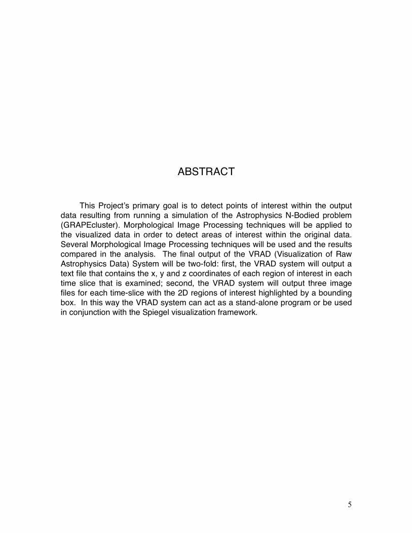
ABSTRACT

This Project’s primary goal is to detect points of interest within the output data resulting from running a simulation of the Astrophysics N-Bodied problem (GRAPEcluster). Morphological Image Processing techniques will be applied to the visualized data in order to detect areas of interest within the original data. Several Morphological Image Processing techniques will be used and the results compared in the analysis. The final output of the VRAD (Visualization of Raw Astrophysics Data) System will be two-fold: first, the VRAD system will output a text file that contains the x, y and z coordinates of each region of interest in each time slice that is examined; second, the VRAD system will output three image files for each time-slice with the 2D regions of interest highlighted by a bounding box. In this way the VRAD system can act as a stand-alone program or be used in conjunction with the Spiegel visualization framework.

6

TABLE OF CONTENTS

1. Introduction

2. Problem Statement and Research Objective

3. Literature Review

4. Design

4.1 Architecture

4.2 Input

4.3 Output(s)

4.3.1 Text file

4.3.2 A Series of Time-Stamped Images for XY, XZ and YZ

Views

5 Implementation Details

5.1 Data Representation

5.2 Higher Level Implementation Details

5.3 Lower Level Implementation Details

5.3.1 VRAD

5.3.2 Parse script

5.3.3 Getdata

5.3.4 Morph

5.3.5 Run

5.3.6 Zerotxt

7

5.3.7 Postpro

5.4 Overall Picture – GRAPEcluster and Spiegel

6 Results

6.1 Type of Particle and View (Gas)

6.1.1 For Gas Top (XY)

6.1.2 For Gas XZ

6.1.3 For Gas YZ

6.2 Other Types of Particles

6.2.1 Star

6.2.2 Cloud

6.2.3 Dark Matter

6.3 New Methodology vs Old (a comparison)

7 Discussion/Comparison and Implications

8 Research Dependencies

9 Future Work

9.1 VRAD – Further Optimizations

9.2 Spiegel – Visualization Framework

9.3 GRAPECluster – Interactivity

10 Conclusions

11 Works Cited

Appendix: Deliverables

8

A) VRAD – overall system (UNIX script)

B) Parse script – parse out useful info from text file (UNIX script)

C) Getdata – convert from text to image (MATLAB code)

D) Morph – perform morphological operations (MATLAB code)

E) Run – perform getdata and morph on a set of files (MATLAB code)

F) Zerotxt – text overlaid on image (MATLAB code)

G) Postpro – post-processing (MATLAB code)

9

1. INTRODUCTION

The Astrophysics N-Bodied problem is one where we wish to study the interactions between N particles in a system. These interactions are governed by Astrophysical laws and properties and can be calculated. However, as N gets larger the number of calculations that must be made in order to accurately represent these values grows exponentially. Since every particle exerts a force on every other particle the complexity of the computation is O(N2). Since a rather large amount of data is produced by this simulation, we wish to have a way to focus on areas of interest that may be present in the data collected. Close to 40GB of data related to the N-Bodied problem has currently been collected using the Grape Cluster hardware/software. One of the goals of this project is to find the temporal and/or spatial correlation between sets of data in connected snapshots over time. This will be achieved by using various morphological techniques such as majority, open and close operations, in image processing including open and close and comparing their results with the current approach of applying computer graphics techniques such as skeletonization and splatting [1]. Once we locate the areas of interest from within the visualization system, we wish to go back and see what this tells us about the structure of our data. MATLAB has a number of built in functions that can aid us in our endeavor to analyze the data to pick out the pieces of information that are important. Since 40GB is simply too large a data set to be able to visually represent everything, it is our hope that the analysis of the data in this way will yield useful results that can be applied in general to the raw data in order to illuminate areas that are of interest. The VRAD (Visualization of Raw Astrophysical Data) system will take the data (or visualization of the raw data for simplification) and identify areas of interest within the image visualized. In order to do this we must define what we think is “interesting.” Within this context, “interesting” refers to a collection of particles that occupies a relatively small region of the image and appears to be having very close interactions between the particles that are members of the object. This information is important to us, so that we can further analyze the nature of the particles’ interactions. For example, is a new galaxy forming? Do we have some anomalous astrophysical event occurring? If so, this section of the data can be further analyzed by astrophysicists to yield new information about the nature of galaxy interactions. Since the data itself is keeping track of particles for each time-slice, this lends itself well to the above-mentioned analysis. What ends up happening is we see a connection forming between the particles in one time-frame and another. Sometimes this change will be great enough for the system to lose interest in a region of space for a time, other times the interactions will cause one region

10

which was previously uninteresting to become of interest. We wish to be able to classify objects of “interest”. If we apply the morphological operations on a black and white image we can classify objects within the visualized data. The morphological operations discussed below perform bit operations on a black and white image that is the result of converting the original image or plot generated from the GRAPEcluster data, into a black and white image that will consist of “on” bits and “off” bits (ones and zeroes). Based on this, we generate new images that we can then perform connected component analysis on to discover our areas of interest. This classification scheme is heavily dependent upon which morphological operations are applied and in what order. The issue of Data Scaling will need to be addressed. When something out of ordinary happens we may define this to be of interest. Some interesting events may be the interaction of several particles, the clustering of particles together or the movement and tracking of particles over time. As a “proof of concept” the demo for this system included the following process: read image file in that is the output of the Spiegel visualization system, convert to binary image with pixel values 1 and 0, perform morphological operations, dilate, label the resulting objects in the image, draw bounding box around resulting objects in image, overlay bounding box over original image, showing focus of attention. Do this for each frame represented by approximately 400 .png images. Write the output images into a directory and create a movie based upon those output images. The final deliverable for this Project will read in the raw Astrophysical data itself (that is the output of the GRAPEcluster Simulation) and graph that data in three dimensions to show not only the length and width of what is deemed interesting, but also how deep the interesting event occurs. Another property to investigate in this project is to look at the interaction between particles over time. This may also be of interest. For the purposes of this Project focusing on a subset of the problem of “interest” which is find interesting gas formations. This can later be expanded upon once we can better define what we find interesting. A more thorough and complete analysis of the four-dimensional data is mentioned as a possible future direction for this research. One advantage of this approach is that it is useful for tracking local phenomena meaning areas of interest that are confined to a relatively small dimensions as opposed to interesting events that may be occurring over a large area of the image. One way to possibly work around that issue is to use a different combination of morphological operators in order to get a different labeling of our objects of interest. Another possible area of investigation would be to process the image at different scales.

11

The VRAD (Visualization of Raw Astrophysics Data) system will fit into the overall framework of the Grapecluster and Spiegel visualization system as follows:

Figure 1.1: VRAD in the overall GRAPEcluster and Spiegel framework The Input to the VRAD system is the output data from the GRAPEcluster N-body simulation. This data is then analyzed using the morphological techniques to yield positions that we can then focus a camera on in the Spiegel visualization system.

Input Data Extractor

VRAD

Visualizer Camera

12

2. Problem Statement and Research Objective

Throughout this research the overall objective would be to create an overall system for visualization of Astrophysical Data in which the user would be able to control the visualization and simulation. This would build upon some existing technology in the field for visualizing this data and would also incorporate novel techniques in the field of Image Processing and Artificial Intelligence in order to gain useful information from and visualize that data. The research conducted will apply towards the entire chain of the system, from the initial conditions put in by the Astrophysicists to the N-Body simulator itself. The output of the GRAPE cluster is then analyzed by my current work (VRAD) and the output of that system is sent to the Spiegel visualization system written in Java (jogl). The output is in the form of x, y and z coordinates and time t. This data is used to focus a camera on this spatial-temporal location.

While the overall objective and goal of this research is visualization, the

system will have two tangible outcomes. The first is in the form of an output file that will contain the location of the regions of interest for each time-slice. The output file will contain the object number, time, x position, y position, z position, x length, y length and z length. With this information we can plug-in to a visualization framework that was built specifically for observation of Astrophysical data. With this information we can track and follow an object over time to see what information this reveals to us about galaxy formations and possibly Astrophysical phenomena. In this way the system acts as an add-in to a larger system. However, VRAD can also act as a stand-alone system that can be used to visualize the raw data itself, once GRAPE Cluster has produced output. The VRAD system identifies objects of interest in images that are mapped from thee-dimensional space and we can use the resulting images that are generated to produce a time-sensitive movie of the evolution of particle interactions.

We want to apply image morphological processing techniques (such as Majority and Dilate) to the idea of object recognition of interest in Astrophysical data. If we can do this, then we have successfully applied known techniques of image processing to a known area, in a novel way. It is the hope that if we can do this, we can reveal more information about the inner structure of the data than previously.

13

The planned way in which Research will be conducted for this project will

be as follows: First off, there will be a review of relevant literature in the field as discussed above. Next we will run experiments of the system and test it’s relative effectiveness when pointing out objects of interest by examining the output of the system. The system will, by default, also do some visualization while the main output of the system will a text file that is used by another component to focus a camera on a region of interest. With this internal visualization we will be able to empirically determine the correctness of our methods. Since “Interest” is a possibly debatable terms, we may need to define more clearly what exactly constitutes an area of interest in order to make more valid claims as to the correctness of the system. However, at this juncture a merely subjective approach may be equally valid for preliminary testing purposes. That is to say that we can determine if something is or is not “of interest” and then go from there.

In addition, one method of methodological verification will come when we

resent our findings to the Astrophysicists themselves and they tell us whether the results are truly “of interest” or if some of the results were anticipated. It may be helpful to present some sort of confusion matrix of identification objects as interesting, where mislabeled objects that are false positives are in one field and false negatives in another.

14

3. LITERATURE REVIEW In the Campanelli paper [1], the authors formulated a problem in the field of Astrophysics related to the study of “fully nonlinear and pertubative evolutions of non-rotating black holes with odd-parity distortions.” The paper is a scientific one and thus it is most likely that a quantitative approach is employed since the scientific method is one example of a quantitative approach. Even more that that there appeared to be a great deal of mathematical formulation and solving in the paper and that, too, is related to the quantitative research methodology. The main research question being asked in this paper by the authors would seem to be: “what are the results of nonlinear perturbative evolution of black holes?” Through a complex analytical analysis and computation, the authors arrive at a conclusion. [1].

The authors’ research orientation clearly seems to be quantitative and concerned with the scientific method for discovery and analysis. The authors solve subsets of a mathematical problem in astrophysics based upon similar methods of their predecessors mentioned in the “literature review.” The paper does appear to be internally consistent with itself.

This question is fairly interesting for this paper due to the fact that like the other paper, it is very difficult to gain any actual empirical evidence for the correctness (or incorrectness) of a particular theory or hypothesis. Instead simulations are often run given a set of initial conditions and then the output is compared to our hypothesis to see if the original hypothesis was correct. The problem inherit in this approach is that it may be the case that the simulation itself is incorrect. That is to say there may be some artifacts in the way that the simulation was coded that may be showing us something that is not there. Nonetheless, again there exists a very close relationship between the theoretical and research perspectives since they are intrinsically connected with one another.

The authors do indeed evaluate and mention other relevant literature related to the topic covered in the paper. They mention methods described by other authors in formulating the complex set of mathematical equations needed to understand the data. Specifically mentioned are odd-parity and even-parity distortions and more complete coverage of these topics in other papers. Additionally things like the Einstein equations decomposition and other methods are described by the authors as standard practice for interpretation of these types of equations.

The paper is well, written and does successfully reference several other papers that one might want to read as well in an effort to more fully understand all the equations and mathematics that go into solving such a complex set of

15

equations. This paper, I believe, takes a step in being able to understand more about the nature of black holes. The more subsets of this problem that can be solved in a similar manner, the more we will begin to understand black holes and the nature of the universe. [1]. The authors of [10] do a good job of some basic astrophysics that is relatively accessible to someone like myself. Unfortunately, as mentioned in another question no specific references are included in this background areas, presumably because any real astrophysicist would be intimately aware of the sets of equations that are being used here. Even though this paper was written back in 1992, many of the ideas and methods employed are still helpful and relevant to the other new work that I have seen in the area. [10]. For reference [2], this is not a paper but an overall project spearheaded by Dr. Hans-Peter Bischof in the Computer Science department and involving members of the Physics department such as Dr. Stefan Harfst and Dr. David Merritt. A Dedicated Parallel Platform for Astrophysical Dynamics. One of the most CPU-intensive calculations in astrophysics is the gravitational N-body problem, in which a set of N particles representing stars move in response to the gravitational force generated by the N-1 other particles. The problem is hard because the number of interactions scales as O(N2), and because stars often form tightly-bound binary systems requiring short time steps. The state-of-the-art way to deal with the N-body problem is via special-purpose computers called GRAPEs (GRAvity PipEline). They are manufactured in Tokyo by the Hamamatsu Metrix Corporation .

The GRAPE boards compute the inverse-square force for large numbers of particles simultaneously, at speeds greatly in excess of a general-purpose supercomputer.

The next step in special-purpose hardware for the gravitational N-body problem is the GRAPE cluster, a Beowulf cluster in which each node is connected to a GRAPE accelerator board. The largest such cluster, comprising 32 nodes, has recently been constructed at the Rochester Institute of Technology by David Merritt in the Department of Physics in collaboration with Dr. R. Spurzem of the Astronomisches Rechen-Institut at the University of Heidelberg. Called "gravitySimulator," this computational platform runs at 4 Tflops, making it one of the fastest computers in the world at the time [2]. Reference number 4 in our works cited list is not a paper, however with the addition of Ed’s work, much has been done in the area of visualizing the N-Body astrophysics problem. This area of research would most likely fit under Relevant tab. With this software addition it became possible to visualize the data in new and interesting ways and made future work in the area of visualizing N-Body data possible. [4].

16

The GRAPEcluster Project is a group of students, postdocs and faculty from the astrophysics and computer science departments who meet once a week to work together on problems relating to the GRAPE cluster. Topics under discussion include algorithm development; visualization software; and scientific research, focusing on the formation and evolution of galactic nuclei and supermassive black holes. [2]. Paper [3] deals with several portable and relatively efficient implementations for the N-Body methods including the Fast Multipole Method, a more adaptive version of Anderson’s Method and the Barnes-Hut method that is also mentioned in other literature which I have read. The program is based on a distributed system. This allows one to break down the problem and use a “divide-and-conquer” approach. [3]. The authors employ the Barnes-Hut Method and Fast Multipole Methods as well as previous literature in the field. The difference in this paper is that they exploit temporal locality in order to obtain more optimal network efficiency when on a distributed system. [11]. Paper [5] deals specifically with the area of research that I wish to focus on: Visualizing N-Body Data in a novel way. This paper uses the computer animation techniques of skeletonization and splatting in order to visualize the inner structure of this data. The hope is that by visualizing the data in this way, we can further examine astrophysical phenomena thought to be present in the data. The approach described as applied to the specific domain in this way is a novel approach to the astrophysics N-Bodied problem as there are few similar hardware/software simulations available to begin with, let alone the specific way outlined below to analyze the data. Thus, almost any venture in the field would automatically be the exploration of an open problem. Visualization Analysis of Astrophysics N-Bodied Problem using Image Morphological Processing Techniques in 3 Dimensions. The goal of his approach would be to detect points of “interest“ within the output data resulting from running a simulation of the Astrophysics N-Bodied problem using the GRAPEcluster hardware/software [2]. The application of Morphological Image Processing techniques will be applied to the visualized data in order to detect areas of interest within the original data. Several Morphological Image Processing techniques will be used and the results compared in the analysis. The final output of the system will be the x, y and z coordinates of regions of interest and the x-width, y-width and z-width of the parallelepiped that can then be used by Spiegel to focus the camera on.

17

The Astrophysics N-Bodied problem is one where we wish to study the interactions between N particles in a system. These interactions are governed by the Astrophysical laws and properties and can be calculated. However, as N gets larger the number of calculations that must be made in order to accurately represent these values grows exponentially. Since every particle exerts a force on every other particle the complexity of the computation becomes O(N2). Since a large amount of data is produced by this simulation, we wish to have a way to focus on areas of interest that may be present in the data collected. Close to 40GB of data related to the N-Bodied problem, has currently been collected, using the Grape Cluster hardware/software. One of the goals of this project would be to find the temporal and/or spatial correlation between sets of data in each snapshot over time. This will be achieved by using various morphological techniques in image processing and comparing their results with the current approach of applying computer graphics techniques such as skeletonization and splatting. Once the areas of interest are located, from within the visualization system, we wish to go back and see what this tells us about the structure of our data. MATLAB has a number of built in functions that can aid us in our endeavor to analyze the data to pick out the pieces of information that are important. Since approximately 40GB is simply too large a data set to be able to visually represent everything, it is our hope that the analysis of the data in this way will yield useful results that can be applied in general to the raw data in order to illuminate those areas which are of interest. The VRAD system takes the raw data output from the GRAPEcluster simulation and identifies areas of interest within the image visualized. There is also the capacity within the VRAD system to take image files previously generated from the Spiegel visualization framework and perform the same analysis on them. In order to do this we must define what we think is “interesting.” Within this context, “interesting” refers to a collection of particles that occupies a relatively small region of the image and appears to be having very close interactions between the particles that are members of the object. This information is important to us, so that we can further analyze the nature of the particles’ interactions. For example, is a new galaxy forming? Do we have some anomalous astrophysical event occurring? If so, this section of the data can be further analyzed by astrophysicists to yield new information about the nature of galaxy interactions. If we can keep track of individual units across time-slices, this will lend itself well to future analysis. We wish to be able to classify objects of “interest”. If we apply the morphological operations on a black and white image we can classify objects within the visualized data. The morphological operations discussed below perform bit operations on a black and white image that is the result of converting the original image or plot generated from the Grapecluster data, into a

18

black and white image that will consist of “on” bits and “off” bits. Based on this, we generate new images that we can then perform connected component analysis on to discover our areas of interest. This classification scheme is heavily dependent upon which morphological operations are applied and in what order. The issue of Data Scaling will need to be addressed. In Saliency and Novelty detection events will happen that happen a lot. When something out of ordinary happens we may define this to be of interest. Some interesting events may be the interaction of several particles. [5]. The authors of paper [6] report on astrophysical N-Body simulation performed with a treecode on a 32 pipeline processor specialized for gravitational force calculations: the GRAPE-5 (Gravity Pipe 5) system. The paper performs calculations based on an N-Body simulation with 2.1 million particles and achieves a performance of 5.92 Gflops average over 8.37 hours. [6]. The authors of paper [7] also employ a similar approach to that of [10]. The paper makes mention of a variety of methods dealing with the N-Body problem in Astrophysics. The paper mentions recent discovery of methods involving a tree structure that can be built and maintained across a networks so that the problem can be more easily parallelized and a “divide-and-conquer” approach may possibly be employed [7]. The results were comparable to those obtained in the Warren/Salmon papers [10]. This paper would best fit under the Overview Papers tab. This paper reviews some relevant methods for being able to visualize the results of a scientific or engineering problem. The paper breaks down the taxonomic specifications between the scientific opportunities involved in modeling things like molecules and brain structure and more engineering oriented problems such as computing fluid dynamics. The findings that different types of visualization are required for different tasks may seem fairly obvious, however it is an important distinction to make. We should endeavor to create the right kind of visualization model for the experiments that we run. The impact that this could have on my future work will include the classification of the kind of problem that we are really dealing with when speaking of the N-Body problem, thus being able to provide the most suited visualization techniques. [8].

The authors, Warren and Salmon, formulate a well-known problem within the field of Astrophysics: The N-Body problem. The real underlying problem with trying to discover knowledge about astrophysics lies in the fact that it is impossible to conduct direct experiments on galaxies themselves, as the authors point out. Rather, scientists have to build models and simulations and test their theories and hypotheses on those. The overall significance of this issue is relatively clear since the authors chose to attack a well-known problem and then

19

present the results in terms of how much processing power they were able to get out of the hardware they chose to run the simulation on.

Quantitative research is much more applicable for this discipline, especially within the context of the Scientific Method. One possible hypothesis (although it is not completely clear) may be that through supplying the correct Initial Conditions to the equations representing Newtonian Gravity, one can effectively know how the formation of galaxies occurs in the cosmos. To this effect the authors further explain that they are setting out to test a procedure for parallelizing the computation of approximations of astrophysical equations. These approximations are already known and it is primarily the author’s intent to show the procedure and results that they have obtained, than to go about making and testing a given hypothesis about the formation of galaxies. It is conceivable that future papers that would use this work, have make and tested hypotheses related to the formation of galaxies and have determined whether that original hypothesis was correct, however that does not seem to be the goal here.

The authors’ research orientation is quantitative in nature. Measuring and observing astrophysical phenomena and using those observations as inputs to a simulation would fit under the quantitative approach. The way that the authors approach the quantitative research orientation appears, at least within the context of the paper, to be internally consistent with itself. That is to say there does not appear to be any point when the authors are claiming to be using more a qualitative approach, nor does it seem that they are in any way misrepresenting themselves or their data quantitatively, since they run the given simulation on the machines they have at their disposal and arrive at a number of computations per second.

For the purpose of this paper the relationships between the research and theoretical perspectives are intrinsically tied to one another. This means that the whole reason for testing out a particular hypothesis in the simulation is to verify it’s validity in accordance with the present theory at the time. Since we cannot run experiments on galaxies (as the authors state) since that would take billions of years to empirically verify the hypotheses that we are attempting to verify, we must therefore use the simulation given a set of initial conditions and compare the results of the simulation with the theory or hypothesis.

While there is no section set aside specifically for reviewing relevant literature within the field that the authors are studying, the authors do evaluate and reference some literature related to the topic at hand. Interestingly enough it seems that most of the literature discussed is on the simulation/computing side related to the problem of astrophysical simulation, while the actually physics background information is discussed but no reference information is included as to the source of such information. Perhaps it is because a general familiarity

20

among the scientific community in regards to the problem is assumed for anyone who will be reading this paper (published in IEEE). In any case the authors do at several points make mention of other similar simulations or experimentations that are also in the fields. One interesting mention of another paper includes on page 574 when the authors decide to run further simulations based upon the annunciation of the “microwave background anisotropy” by the COBE satellite that is mentioned by two other papers. So, apparently with this new information, the authors are able to form more completely the set of input parameters for the simulations.

The basic components of this study design seem to be as good as they can be given the situation that we are dealing with: Trying to simulate the complex formation of galaxies over the course of billions of years. The authors make light of this somewhat in section one where they say that “Astrophysics is at a disadvantage to some of the more terrestrial sciences … An investigator can easily change the recipe for making a superconductor. On the other hand, the recipe for making a galaxy requires 1045 grams of mater, and several billion years of ‘baking’ … With numerical methods, however, one can simulate the behavior of 1047 grams of matter over a span of 1010 years. The accuracy and validity of the measurements comes into play in the simulations as well since we cannot directly empirically observe anything cosmologically in these experiments all the observations must be made from the simulations themselves. These authors are primarily concerned with being able to run the simulation in an effective and efficient manner. In the section where the authors analyze the run-time of recent simulations they analysis of the data seems to be fairly accurate and thorough. The authors go through the trouble of specifying how many flops each interaction costs on a small scale for each kind of computation. However, there may be some overhead factors that are not explicitly taken into consideration. The measurements are in terms of FLOPS (floating point operations per second) and according to the authors are measured by internal diagnostics compiled by the program (the simulation, presumably) when run. Thus, if set up correctly these, measurements should be rather precise. The analysis of the date is therefore relatively accurate and relevant to the research question at hand. The conclusions of this paper seem to be valid and consistent with the metrics and measures of performing the research. The authors make mention of possible future work including limitations of the current code and the possible presence of new (i.e. better) numerical techniques being developed for future application and analysis.

In my opinion the authors do use an element of emotion in the paper that I feel adds to the overall feel. For example on the first page the authors say: “… the recipe for making a galaxy requires 1045 grams of matter, and several billion years of ‘baking,’ which is far beyond the patience of most scientists. This sort of tongue-in-cheek example of gently poking fun at other disciplines as being

21

easier to analyze and test theories for is prevalent throughout the paper. The use of this kind of humor is used sparingly enough to add something to the paper without distracting from its overall message, I feel. The authors also obviously feel very passionately abut this project by the first sentence of section one: “The process by which galaxies form is undoubtedly among the most important unsolved problems in physics.” This really leaves little room for interpretation, however it is likely that this is true anyway and that most scientists would agree with this point. In his paper [5], the author describes how to visualize the inner structure of N-Body data using computer animation techniques of Splatting and Skeletonizaion. The goal of this work was to visualize Astrophysical Phenomena that is thought to be present. Splatting is a technique used for volume rendering that is similar to ray tracing, only in three dimensions. Splatting can be conceptualized as the flattening of a three dimensional voxel onto a two-dimensional image plane. With Splatting each voxel is projected onto the image plane using a Gaussian kernel function.

With Skeletonization, the aim is to portray the “essential topology” of an object by preserving the elemental structure of an object and leaving out many of the details. Skeletonization of a rectangle would include a skeleton shape representative of the length with branches into each of the four corners. With Skeletonization, however, some unwanted artifacts of the data emerged that would not be wanted in a visualization of the data. The approach of drawing a bounding box around objects of interest is not a new one, but has been used in image processing fields for quite some time. In fact in a thesis paper by Paskali [9], the author uses a means of object tracking and draws bounding boxes around the regions of interest based upon biological models of attention and novelty. In the author’s examples he is mostly interested in the motion of people and vehicles in order to determine what is novel in the scene [9].

22

4. DESIGN

4.1 Architecture

The overall architecture of the system is as follows: a UNIX script aptly titled “vrad” is used to invoke the system. The script contains first another UNIX script named “parse” that parses through the input text file that is the output of the GRAPEcluster simulation. The “parse” script reads from a specific location where the GRAPEcluster output data is currently stored and filters out only the x, y and z information for a specific type of particle over a user-specified time interval. The output of this script is a new file which is stored locally and is smaller in size than the original.

Next “vrad” executes the command “matlab –r “run;exit” ” which

runs the MATLAB in command-line mode. The MATLAB file run contains two other MATLAB functions that are to be executed: getdata.m and morph.m. Getdata takes the file created by the parse script and converts it into an .png image file based upon a 2D projection of the 3D space represented by the data file. This is done in the XY, YZ and XZ dimensions in order to obtain three image files for each time interval represented in the input data.. Next, Morph.m takes the image files created by Getdata.m and runs a set of morphological operations on them to determine the areas of interest for each separate image. The output of this function is twofold: first, a text file with each line corresponding to the x, y and z data as well as the time index from which the area of interest was detected; second another image for each of the XY, YZ and XZ views with the specific area of interest bounded by a rectangle. In this way we can combine the output images for each view (XY, YZ and XZ) to created a timed movie and visualize how the areas of interest change over time.

The Morph.m file also includes a function that is used to overlay the

time stamp information onto the image, which is useful so that the user can see the time interval and interactions of particles at specific time indices.

From here the system executes a post processing function in

MATLAB named postpro.m that takes the output file created by the Morph.m function and implements object tracking.

23

In this way the system is unique in that it can either act as a stand-alone program merely taking in the input as the output of the GRAPEcluster simulation and then producing visualizations with the areas of interest highlighted in each time frame or it can be incorporated into the overall Spiegel visualization framework add-in as mentioned above. This is accomplished by reading in the output file created by VRAD into Spiegel and pointing the camera at the spatial location specified [2].

4.2 Input The Input to the VRAD system, as mentioned above is the text file

output from the GRAPEcluster simulation. This file contains information related to dispersion of four different types of particles in three-dimensional space. The four types of particles are: Star, Cloud, Gas and Dark Matter. For the this analysis, we look at one type of particle at a time (i.e. for a given execution of the VRAD system). There is an output file for each time-slice from the GRAPEcluster. Within each file, each particle is represented by a line showing the various attributes of the particle. id mass x y z … ipt … 1 1.7039E-05 -8.3096E+00 -7.9625E+00 1.7795E-01 … 1 … 2 1.6828E-05 -1.2659E+01 -1.0378E+01 6.5997E-03 … 1 … 3 1.7101E-05 -2.1093E+01 -1.2123E+01 -5.1354E-01 … 1 … 4 1.6908E-05 -2.3068E+01 -6.2324E+00 1.7259E-01 … 1 … 5 1.7012E-05 -1.8001E+01 -9.9293E+00 -3.0026E-01 … 1 … . . . 445435 1.9363E-05 3.5438E+01 1.0143E+01 -7.5912E-01 … 4 … 445436 1.9363E-05 1.0301E+01 -4.8686E+00 4.7373E+00 … 4 … 445437 1.9363E-05 1.5090E+01 2.3221E-01 1.7954E+00 … 4 … 445438 1.9363E-05 3.5675E+01 -1.2064E+01 9.5013E+00 … 4 … 445439 1.9363E-05 1.9877E+01 7.3966E+00 4.8282E-01 … 4 …

24

4.3 Output(s)

As mentioned previously mentioned the output of the VRAD system is two-fold: first the VRAD system will output a text file that contains the x, y and z coordinates of each region of interest in each time slice that is examined; second, the VRAD system will output an three image files for each time-slice with the 2D regions of interest bounded by a bounding box. In this way the VRAD system can act as a stand-alone program or be used in conjunction with the Spiegel visualization framework.

The text file is of the following form: field one is the unique object identifier,

field two is the object number which is tracked over different time indices, field three indicated whether an object has come from the splitting or merging of another object, field four is the view (XY, YZ or XZ), field five is the time index, field six, seven and eight are the x, y and z starting positions that bind the object of interest, fields nine, ten and eleven are the lengths in the x, y and z dimensions of the bounding region. The text file looks like this: ( “outputfile.txt” ):

1 XY 00000 33.71 -3.14 0.03 26.57 26.57 5.48 2 XY 00000 -6.29 -23.14 0.03 26.57 26.57 5.48 1 XZ 00000 33.71 0.03 -4.29 26.57 5.48 8.29 2 XZ 00000 -6.29 0.03 -4.00 26.57 5.48 8.00 1 YZ 00000 0.03 24.29 -5.14 5.48 47.71 10.00 1 XY 00005 32.29 -2.86 0.03 26.00 26.57 5.48 2 XY 00005 -5.43 -23.43 0.03 26.86 27.43 5.48 1 XZ 00005 33.43 0.03 -4.00 27.43 5.48 8.57 2 XZ 00005 -5.14 0.03 -4.00 27.43 5.48 10.86 1 YZ 00005 0.03 24.00 -4.29 5.48 47.71 9.71 . . . 1 XY 02000 30.00 -24.29 0.03 4.00 4.00 5.48 2 XY 02000 19.14 -12.57 0.03 34.00 27.43 5.48 1 XZ 02000 42.86 0.03 -1.43 3.71 5.48 3.71 2 XZ 02000 32.57 0.03 -2.57 6.86 5.48 4.29 3 XZ 02000 19.43 0.03 -4.86 34.86 5.48 8.57 1 YZ 02000 0.03 33.14 -1.71 5.48 4.29 4.00 2 YZ 02000 0.03 26.00 -1.43 5.48 3.71 3.71 3 YZ 02000 0.03 16.86 -3.43 5.48 33.43 7.43 4 YZ 02000 0.03 -20.29 -2.57 5.48 7.14 4.86

25

Another output file is created that specifically deals with the output tracking in the XY plane: ( “object” ):

id obj from view t x y z xlen ylen zlen 1 1 0 XY 00000 33.71 -3.14 0.03 26.57 26.57 5.48 2 2 0 XY 00000 -6.29 -23.14 0.03 26.57 26.57 5.48 3 1 0 XY 00005 32.29 -2.86 0.03 26.00 26.57 5.48 4 2 0 XY 00005 -5.43 -23.43 0.03 26.86 27.43 5.48 5 1 0 XY 00010 32.57 -2.86 0.03 27.14 26.86 5.48 6 2 0 XY 00010 -4.86 -22.86 0.03 26.86 27.14 5.48 7 1 0 XY 00015 31.71 -3.14 0.03 27.14 27.71 5.48 8 2 0 XY 00015 -4.00 -22.86 0.03 27.43 27.71 5.48 9 1 0 XY 00020 31.14 -2.86 0.03 27.71 28.00 5.48 10 2 0 XY 00020 -3.43 -22.86 0.03 27.71 28.00 5.48 . . . 1722 612 0 XY 01990 18.57 -8.00 0.03 3.71 4.29 5.48 1723 613 0 XY 01990 13.14 -16.00 0.03 28.29 31.14 5.48 1724 614 0 XY 01990 0.57 30.29 0.03 3.71 3.71 5.48 1725 599 0 XY 01995 28.86 -25.14 0.03 4.00 4.57 5.48 1726 612 0 XY 01995 18.86 -6.86 0.03 4.00 4.29 5.48 1727 613 0 XY 01995 15.14 -15.71 0.03 30.29 30.57 5.48 1728 614 0 XY 01995 0.00 29.71 0.03 4.00 4.00 5.48 1729 615 0 XY 01995 -40.86 -0.29 0.03 4.00 3.71 5.48 1730 599 0 XY 02000 30.00 -24.29 0.03 4.00 4.00 5.48 1731 616 613 XY 02000 19.14 -12.57 0.03 34.00 27.43 5.48

This file is used as input to the Spiegel visualization framework in order to focus the camera on a specific region of interest for a duration of time. For example, suppose we had a region of interest that existed for the first 25 frames of data, we would want to focus the camera on this region during the time when the region was considered interesting by the system. Sometimes what ends up happening is that due to the reclassification of objects over time, the system looses interest in one object, however another object becomes interesting. This happens when a splitting or merging of particles occurs. When this happens we want the system to be able to identify the new region of interest as being closely related to the previous region of interest, as opposed to a whole new region. This is done by comparing the size and location information derived from the data, to the

26

previously recorded information. If the data matches above a certain threshold, we can safely classify the new region as a continuation of the previous one. If not, then we label it as a truly new region and the Spiegel visualization framework would devote a new camera to focus on this region.

In addition to the text file Image files created by application of morph on the output of the getdata images are created for each data file:

Figure 4.1: Image with bounding boxes around regions of interest

27

Figure 4.2: VRAD architecture

VRAD

Run

Morph Getdata

Parse

Postpro

Zerotxt

28

Figure 4.3: VRAD’s Output

This figure shows the output from the GRAPEcluster simulation being fed in as the input to VRAD. Then VRAD produces two outputs. The first is a text file that shows the locations of regions of interest over time. This text file is read in by a script and converted to a form that can be read in as input to the Spiegel visualization framework. The input directs the placement and movement of cameras within Spiegel to focus on the interesting events. The second output of VRAD is a series of time-indexed images that are assembled according to the time-stamp information, into a movie file. By looking at the movie file we can begin to gain an understanding about the structure of the simulation data.

Data

VRAD

Text file Images

Script Movie

Spiegel

Camera

29

5. IMPLEMENTATION DETAILS 5.1 Data Representation For a problem of this nature it is helpful to have an idea how the data that we will be working with is formulated and laid out. Field identifier Description

Id Particle index starting from 1 (not unique across time slices)

Mass Particle mass (may not be constant)

x, y, z Particle position

vx, vy, vz Particle velocity in x, y and z directions

Pot Potential

H Particle radius (undefined for stars and dark matter)

U Internal specific energy (gas particles only)

Rho Mass density of the gas at the position of particle (gas and

cloud particles)

T Temperature, or same as rho

Tob Time of birth (when particle first introduced into simulation)

Ipt Particle type: 1 – stars, 2 – clouds, 3 – gas, 4 – dark mater

Icomp Galaxy component: 1 – disc, 2 – bulge, 3 – halo

Igal Galaxy identifier (if two or more galaxies)

Icol Same as ipt

Table 1: Data Representation

30

Figure 5.1: Example Image output of Spiegel visualization system

The above example is one of the output images from the Spiegel visualization system [4].

31

5.2 Higher Level Implementation Details

A) VRAD – overall system (UNIX script)

B) Parse script – parse out useful info from text file (UNIX script)

C) Getdata – convert from text to image (MATLAB code)

D) Morph – perform morphological operations (MATLAB code)

E) Run – perform getdata and morph on a set of files (MATLAB code)

F) Zerotxt – text overlaid on image (MATLAB code)

G) Postpro – post-processing (MATLAB code)

The VRAD can act as either a stand-alone (with respect to the Spiegel visualization framework) or add-on to Spiegel visualization framework. In it’s current state the system accepts an image, or series of images that is the output from the Spiegel visualization system and from that, find the areas of interest within each image. The system can also take the raw data that is generated from the GRAPEcluster simulation. Based upon this information and comparing it to the images generated from plotting the raw data itself over time, the goal is for the VRAD system to output the x, y and z coordinates and approximate x-length, y-length and z-length for a parallelepiped around the region of interest. These coordinates can then be fed to the Spiegel visualization system as camera coordinates to focus on. Additionally a time indicator is included in the image output, so that we know when these interesting events are occurring. For each data file the time is indicated, so we can analyze each one separately. The VRAD system projects two dimensions onto an image file for processing. There are three separate views that are considered, XY, YZ and XZ. Taking into account information in all three dimensions. 5.3 Lower Level Implementation Details

5.3.1 VRAD – overall system (UNIX script)

This is the script that is used to run the system. The command issued is: ./vrad The script runs another UNIX script (parse), opens MATLAB up with

32

the command-line option, does some file clean-up and formatting and then exits.

5.3.2 Parse script – parse out useful info from text file (UNIX script)

This script takes the raw data results from the GRAPEcluster simulation and filters out the unnecessary lines leaving only the relevant data. For this project, we are primarily concerned with Gas particles, and their X, Y, Z positions. 5.3.3 Getdata – convert from text to image (MATLAB code)

Getdata.m is a MATLAB function that takes the new data file(s) written by the parse script and converts maps them to an image file based on the following formula: pixely = round(res*(-1*a(i)-min_a)/(max_a - min_a)); pixelx = round(res*(b(i)-min_b)/(max_b - min_b));

The output of Getdata.m is an image file related to each input data file.

5.3.4 Morph – perform morphological operations (MATLAB code) Morph.m is a MATLAB function that performs the morphological operations or majority and dilate on the input image. Next, using bwlabel to find the bounding box around each object in the image, morph.m takes the coordinates and superimposes them over the original image generated from Getdata.m. In addition, a time indicatior and cross-hairs are overlayed onto each image resulting in one output image with the regions of interested bounded by red rectangles. 5.3.5 Run – (MATLAB code) Run.m is a MATLAB file that perform getdata and morph on a set of files. 5.3.6 Zerotxt - (MATLAB code) Zeroxtx.m is the MATLAB function that is used to superimpose text onto the image. In this case the text indicates the time stamp information originally contained in the data files. 5.3.7 Postpro – (MATLAB code)

33

Postpro.m is the MATLAB function used to connect objects in

the output file “object”. This is used so that the camera in Spiegel can focus on an object for a period of time, until it merges or splits to become another object. In this we VRAD can be used to help track objects of interest over time using the Spiegel visualization framework.

Morph:

1. For each image we wish to analyze, read in image and convert the image to a grayscale intensity image to remove unnecessary color information

2. Convert the grayscale image to a black and white image represented by

1s and 0s to indicate the presence or absence of a particle so that we can then perform the following morphological operations on the images

3. Perform the following morphological operations on the image

o Bothat – performs binary closure (dilation followed by erosion) and subtracts the original image

o Tophat – returns the image minus the binary opening of the image o Clean – removes isolated pixels (individual 1’s surrounded by 0’s) o Close – performs binary closure (dilation followed by erosion) o Majority – sets a pixel to 1 if five or more pixels in its 3x3

neighborhood are 1s, otherwise sets it to 0 o Open – implements binary opening (erosion followed by dilation) o Remove – removes interior pixels – sets a pixel to 0 if all of it’s 4-

connected neighbors are 1, leaving only the boundary pixels on o Skel – removes pixels on the boundaries of objects, keeps object

together o Spur – removes ‘spur’ or peninsula pixels that are otherwise

isolated by 0’s o Dilation – if ANY pixel in input pixel’s neighborhood is 1, the output

pixel is 1, otherwise the output pixel is 0 o Erosion – if EVERY pixel in the input pixel’s neighborhood is 1, the

output pixel is 1, otherwise the output pixel is 0 [6]

4. Analyze results of previous steps morphological operations and then apply the dilate operation (repeat dilation operation, until distinct objects appear)

5. Then apply MATLAB function bwlabel to label the distinct objects that

appear in our image

34

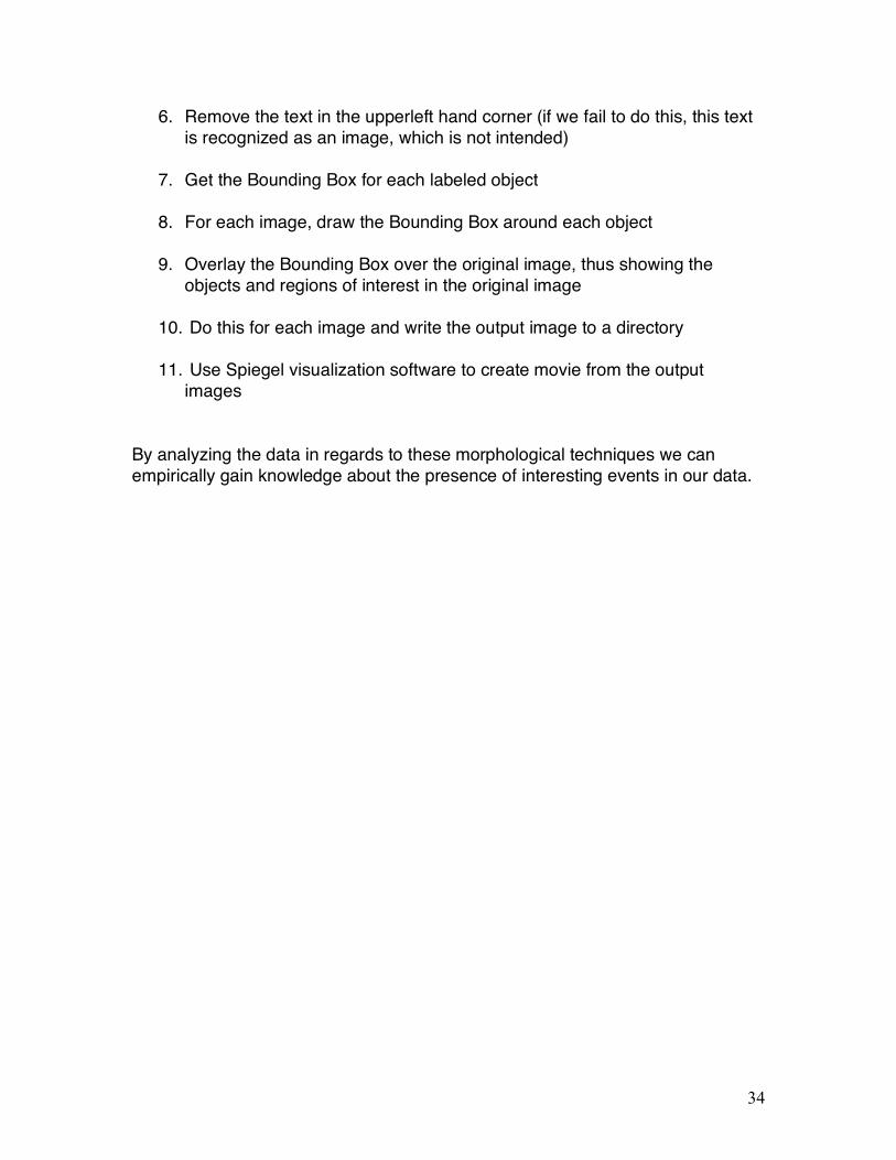
6. Remove the text in the upperleft hand corner (if we fail to do this, this text is recognized as an image, which is not intended)

7. Get the Bounding Box for each labeled object

8. For each image, draw the Bounding Box around each object

9. Overlay the Bounding Box over the original image, thus showing the

objects and regions of interest in the original image

10. Do this for each image and write the output image to a directory

11. Use Spiegel visualization software to create movie from the output images

By analyzing the data in regards to these morphological techniques we can empirically gain knowledge about the presence of interesting events in our data.

35

Figure 5.2: Original Image (generated from Getdata.m)

36

Figure 5.3: output after majority operation performed

37

Figure 5.4: output after Thicken operation performed

38

Figure 5.5: output after Dilate operation applied (six times)

39

Figure 5.5: output after label image is applied and bounding boxes computed

40

Figure 5.6: output after bounding boxes positions are applied to original image

41

Figure 5.7: Majority Morphological Operation applied to test image

42

5.4 Overall picture – GRAPEcluster and Spiegel

The output from the VRAD system can then be utilized by the Spiegel visualization framework in order to point a camera at the region of interest specified in the output file created by VRAD. In addition another object tracking file is included in the output so that when a region of interested is merged or splits with another region of interested the Spiegel visualization framework knows to move the camera to the correct location. Otherwise we would have rather short-lived objects and not as much continuity for object tracking. The output from the GRAPEcluster simulation is the input to VRAD. VRAD produces two outputs. The first is a text file that shows the locations of regions of interest over time. This text file is read in by a script and converted to a form that can be read in as input to the Spiegel visualization framework. The input directs the placement and movement of cameras within Spiegel to focus on the interesting events. The second output of VRAD is a series of time-indexed images that are assembled according to the time-stamp information, into a movie file. By looking at the movie file we can begin to gain an understanding about the structure of the simulation data.

43

6. RESULTS

DELIVERABLES

Deliverables for this Masters Project will include:

• MATLAB code used to perform image processing • Any other code or scripts needed to run the image processing

techniques implemented in MATLAB

• Documentation of MATLAB code and any other tools and utilities used for this project

• Output images resulting from running the MATLAB code

• Output movies generated from output images using Spiegel

visualization software

44

6.1 Gas View

Figure 6.1: Gas particle, XY view

In this view (XY) we can clearly see two distinct regions that represent galaxies comprised of individual particles. As the system is run, the galaxies come closer and close together until they merge and then some of the particles are flung out of the immediate vicinity of the center and form other clusters or particles. It is here that we would look for likely cases to further investigate some of the observed Astrophysical phenomena. Much of the information of revealed by the VRAD system is from this top (XY) view with Gas particles.

45

Figure 6.2: Gas particle, YZ view

In this view (YZ) we see that the vast majority of interesting events occur along a very similarly shaped rectangle. In fact using this view along, it is very difficult to ascertain any usable information about the placement of a camera in three-dimensional space. Where this view helps, is when used in conjunction with information from the other views to obtain a more realistic representation of three-dimensions.

46

Figure 6.3: Gas particle, XZ view

In this view (XZ) we also see that majority of interesting events occur along a very similarly shaped rectangle. In fact using this view along, it is very difficult to ascertain any usable information about the placement of a camera in three-dimensional space. Where this view helps, is when used in conjunction with information from the other views to obtain a more realistic representation of three-dimensions.

47

6.2 Other Types of Particles:

Figure 6.4: Star particle, Top (XY) view

The results when VRAD is used to process data that is filtered to include only star particles is as shown above. The input to the system in this case was the output from the Spiegel Visualization system [4].

48

Figure 6.5: Cloud particle, Top (XY) view

The results when VRAD is used to process data that is filtered to include only cloud particles is as shown above. The input to the system in this case was the output from the Spiegel Visualization system [4]. The output in this case is very similar to that of the Star particles.

49

Figure 6.6: Dark Matter particle, Top (XY) view

Finally, when VRAD is used to process data that is filtered to include only Dark Matter particles only, the results are as shown. Pay particular attention to the lower right hand side of the image. This is where the system detects interesting events. As in the previous two examples, the input to the system in this case was the output from the Spiegel Visualization system [4]. In the case of Dark Matter this technique is completely ineffective since the particles seem to occupy almost all points in our defined space. Some small pockets of Dark Matter are identified in the lower right, however this appears to be more of an artifact of the program than an indication of an Astrophysical phenomena.

50

7. DISCUSSION, COMPARISONS and IMPLICATIONS Using a set of morphological operations for image processing we hope to show that there exists a spatial and temporal correlation between the sets of data that has been gathered from running the GRAPEcluster simulation of the N-Bodied Astrophysics problem. Using this correlation, a future project in this area could include a concentration on investigating why these interesting events are occurring. Once the locations of regions of interest have been detected by the VRAD system, we can use it’s output to feed into the Spiegel framework for the x, y, z and time location to look for events of interest. It is the hope that in doing so we can detect peculiar or anomalous astrophysical phenomena. Using the images generated from previous work in Spiegel visualization, new images with bounding box regions around the areas of interest have been generated. When combined with a time element to form a movie version, we can see how what is defined as an area of interest changes over time. The same is likely to be true for the three dimensional case where we have parallelepipeds surrounding regions of interest in 3D space.

Figure 7.1

This figure was obtained from running the proof-of-concept program created from [9].

51

The author of paper [9] employs this bounding box approach that is fairly common within the field of novelty detection. In this example our areas of interest are defined within the context of a still, image. However, the program itself was designed to operate on a video, i.e. a sequence of images. Based on the differences from one frame to the next the system will track certain objects as being “novel.” This approach, in some ways, parallels that which happens in human visual systems. When presented with a stationary background and a moving object in the foreground, the eye tends to focus on the moving object. The goal of this approach is described in [9] is to “classify the degree of interest of events with respect to previous events in a video stream.” Within this context the degree of interest is associated with how similar an event is compared to some previous event. The higher the similarity between a newly observed event and a previous event, the lower the interest in the new event. Novelty as defined in this system can be understood as a search for something that has never been witnessed before (or has been forgotten). The IVEE system, which stands for Interesting Video Event Extraction is a component of a larger system called VENUS (Video Exploitation and Novelty Understanding in Streams). IVEE focuses assigns a degree of interest for events in the input video stream. The output of IVEE includes the coordinates of said interesting events, the interesting video stream, the memory of interesting events and the missed events list [9]. The approach that the VRAD system takes is different in that in the VRAD system we do not directly look at a sequence of images from a video, but a snapshot of them at one time-slice. An interesting byproduct of this apparent time-independent analysis is that when we do end up looking at two images side-by-side (for example when we create a time-stamped movie file based on the output images) there does appear to be a very strong correlation of position over time. Future work may focus on a more robust implementation of time-sensitive particle movement as well.

52

Figure 7.2 (source [5])

In paper [5], the author chooses a unique approach to visualization of the N-body data, skeletonization. While there is certainly a good deal of merit to this approach, it does, seem to introduce some peculiar artifacts that may lead to an incorrect understanding of the data. Some of the results of this skeletonization produced long, thin “legs” of the galaxies that were not really indicative of the overall structure of the data. In contrast, the approach followed in this project does not have the same kinds of artifacts.

The approach employed in this project is very similar to the Point Rendering approach used by E. Dale [5]. Using that work as a basis, the project includes as one output the two-dimensional Point Rendering for each of the three

53

views (XY, YZ, XZ) for each time-stamped indexed data file. The results produced by the Spiegel visualization and VRAD were nearly identical:

Figure 7.3 Output from Spiegel [5] and output from Getdata.m of VRAD

The above figure shows side-by-side the output from [5] and output from Getdata.m module of VRAD. Notice they are very similar. The other views are also represent this similarity. Note that this is before the timestamp is applied to the image which takes place in zerotxt.m of VRAD.

54

Figure 7.4 Output image Spiegel and VRAD for time index 00500 In contrast is the image above which is the output file resulting from the

same time-slice data as both of the previous images. In figure 7.x above we have two images, the first was generated from the Spiegel Visualization system [4] and then run through morph.m (part of VRAD). The second image was generated from the raw data output of the GRAPEcluster through VRAD. While there are some subtle differences in the final output, the output is fairly consistent. Some of the differences may be a result of scaling.

What we have chosen to implement in VRAD is a special case

dimensional reduction done to reduce the run-time complexity of the overall system. Instead of analyzing the entire three-dimensional space we convert the data given to three separate views representing two dimensions each. We have the XY, YZ and XZ views. When looking at the results of the morphological operations on all three views on one thing that is clear is that there does not seem to be very many objects of interested in both the YZ and XZ views. Where we get the most objects of interest is the XY or top view. Thus, under certain conditions we may be justified in viewing and paying closest attention to this view. There are, however, conditions where this reduction may be inappropriate, such as when we have three-dimensional structure of a sphere and we wish to visualize the center. It would be difficult using this view paradigm to accurately represent the inner structure of the data in the manor. The application of Image Processing and Connected Component analysis within the context of Astrophysical phenomena is, as far as I know, an almost completely open and novel approach to the problem. While other similar simulations have been utilized in the past, it is the data analysis that is different here and the intent is that this analysis will add to our knowledge of the universe.

55

Since there are few similar hardware/software simulations available for analysis of the Astrophysics N-Body problem to begin with and with the novel approach outlined for treating the data as an image, almost any venture into the field would necessarily be the exploration of an open problem. The goal of his approach would be to detect points of “interest“ within the output data resulting from running a simulation of the Astrophysics N-Bodied problem using the GRAPEcluster hardware/software [2]. The application of Morphological Image Processing techniques will be applied to the visualized data in order to detect areas of interest within the original data. Several Morphological Image Processing techniques will be used and the results compared in the analysis. The final output of the system will be the x, y and z coordinates of regions of interest and the x-width, y-width and z-width of the parallelepiped that can then be used by Spiegel to focus the camera on. The Astrophysics N-Bodied problem is one where we wish to study the interactions between N particles in a system. These interactions are governed by the Astrophysical laws and properties and can be calculated. However, as N gets larger the number of calculations that must be made in order to accurately represent these values grows exponentially. Since every particle exerts a force on every other particle the complexity of the computation becomes O(N2). Since a rather large amount of data is produced by this simulation, we wish to have a way to focus on areas of interest that may be present in the data collected. Close to 40GB of data related to the N-Bodied problem, has currently been collected, using the Grape Cluster hardware/software. One of the goals of this project would be to find the temporal and/or spatial correlation between sets of data in each snapshot over time. This will be achieved by using various morphological techniques in image processing and comparing their results with the current approach of applying computer graphics techniques such as skeletonization and splatting. Once the areas of interest are located, from within the visualization system, we wish to go back and see what this tells us about the structure of our data. MATLAB has a number of built in functions that can aid us in our endeavor to analyze the data to pick out the pieces of information that are important. Since on the order of 40GB is simply too large a data set to be able to visually represent everything, it is our hope that the analysis of the data in this way will yield useful results that can be applied in general to the raw data in order to illuminate those areas which are of interest. The system will take the data (or visualization of the raw data for simplification) and identify areas of interest within the image visualized. In order to do this we must define what we think is “interesting.” Within this context, “interesting” refers to a collection of particles that occupies a relatively small region of the image and appears to be having very close interactions between the particles that are members of the object. Particles that are grouped together in

56

this manner may be the result of an astrophysical phenomenon. This information is important to us, so that we can further analyze the nature of the particles’ interactions. For example, is a new galaxy forming? Do we have some anomalous astrophysical event occurring? If so, this section of the data can be further analyzed by astrophysicists to yield new information about the nature of galaxy interactions. Another open-ended question in Astrophysics is “How do galaxies form?” With the GRAPEcluster simulation we can gain a great deal of knowledge relevant to the interaction of these particle within the context of galaxy formations. It is possible, therefore, that this data analysis will yield some Knowledge Discovery. If we can keep track of individual units across time-slices, this will lend itself well to future analysis. We wish to be able to classify objects of “interest”. If we apply the morphological operations on a black and white image we can classify objects within the visualized data. The morphological operations discussed below perform bit operations on a black and white image that is the result of converting the original image or plot generated from the Grapecluster data, into a black and white image that will consist of “on” bits and “off” bits. Based on this, we generate new images that we can then perform connected component analysis on to discover our areas of interest. This classification scheme is heavily dependent upon which morphological operations are applied and in what order. The issue of Data Scaling will need to be addressed. In Saliency and Novelty detection events will happen that happen a lot. When something out of ordinary happens we may define this to be of interest. Some interesting events may be the interaction of several particles. As a “proof of concept” the demo for this system included the following process: read image file in that is the output of the Spiegel visualization system, convert to binary image with pixel values 1 and 0, perform morphological operations, dilate, label the resulting objects in the image, draw bounding box around resulting objects in image, overlay bounding box over original image, showing focus of attention. Do this for each frame represented by approximately 400 .png images. Write the output images into a directory and create a movie based upon those output images. The final deliverable for this Project will read in the raw Astrophysical data itself (that is the output of the Grapecluster Simulation) and graph that data in three dimensions to show not only the length and width of what is deemed interesting, but also how deep the interesting event occurs. Another consideration to make with this Project is to look at the interaction between particles over time. This may also be of interest. For the purposes of this Project focusing on a subset of the problem of “interest” which is find interesting gas formations. Within the context of this research there are 4 types of particles: Star, Cloud, Gas and Dark Matter. For now, the intent is to focus on

57

Gas particles and groupings of Gas particles that are deemed interesting. The interest value is determined by grouping. This can later be expanded upon once we can better define what we find interesting. One side-effect of this approach is that it is most useful for tracking local phenomena meaning areas of interest that are confined to a relatively small dimensions as opposed to interesting events that may be occurring over a large area of the image. One way to possibly work around that issue is to use a different combination of morphological operators in order to get a different labeling of our objects of interest. The projected impact of my intended area of research would possibly be a new understanding of the fundamental ways in which galaxies are formed. By drawing attention to specific regions of interest within our three dimensional space, we can further analyze the interactions between the particles involved and potentially add to the general knowledge of the nature of galaxy formations. Since an exhaustive analysis of all the data points is impractical, the limitation to the further study of only those areas of the data that are interesting will free up time for a more in-depth study of these interactions.

58

8. RESEARCH DEPENDENCIES The Computer Vision and Acoustics Lab (70-3400) in the Golisano College of Computing and Information Sciences at the Rochester Institute of Technology.

• Mac computer with OS X version 10.4.6 o Unix derivative: Darwin 8.0 o Shell: GNU bash, version 2.05b.0(1)-release (powerpc-apple-

darwin8.0) o Dual 1.8 GHz PowerPC G5 o Memory – 2.5 GB DDR SDRAM o Model - PowerMac 7.2 o CPU Type – PowerPC 970 (2.2) o L2 Cache (per CPU) – 512 KB o Bus Speed – 900MHz o Graphics Card – GeForce FX 5200

64 MB VRAM manufacturer: nVIDIA

• MATLAB for Macs version 7.0.0.19901 (R14) • Spiegel visualization framework for GRAPEcluster data Visualization

59

9. FUTURE WORK 9.1 VRAD

Some future work to be done internally with the VRAD system would include further optimizations of selecting areas of interest based upon which type of particle we are looking for. For example, right now the VRAD system is specifically optimized for the detection of interesting Gas particles. Eventually we would like to be able to select which type of particles (or all of the four different kinds) and determine the areas of interest within each segment of particle-types. In order to do this we must first more thoroughly define what we mean by an “area of interest” especially since with particle types such as Dark Matter which seems to have no definitive structure within this data set representation, it is difficult to ascertain which regions are really areas of interest and which are not.

Another advancement to be made on VRAD would be more robust object

tracking that will keep track of the relevant information from frame to frame and be able to track, within a threshold value the probability of an object being in a certain location in the following frame.

As mentioned previously, VRAD does not directly take information from one frame and compare that with the next. Instead we analyze each image file separately. An interesting byproduct of this apparent time-independent analysis is that when we do end up looking at two images side-by-side (for example when we create a time-stamped movie file based on the output images) there does appear to be a very strong correlation of position over time. Future work may focus on a more robust implementation of time-sensitive particle movement as well.

What we have chosen to implement in VRAD is a special case dimensional reduction done to reduce the run-time complexity of the overall system. Instead of analyzing the entire three-dimensional space we convert the data given to three separate views representing two dimensions each. We have the XY, YZ and XZ views. When looking at the results of the morphological operations on all three views on one thing that is clear is that there does not seem to be very many objects of interested in both the YZ and XZ views. Where we get the most objects of interest is the XY or top view. Thus, under certain conditions we may be justified in viewing and paying closest attention to this view. There are, however, conditions where this reduction may be inappropriate, such as when we have three-dimensional structure of a sphere and we wish to visualize the center. It would be difficult using this view paradigm to accurately represent the inner structure of the data in the manor. In future versions of VRAD, we would like to do a true three-dimensional analysis using an analogous three-dimensional version of morphological processing that would involve particles at voxel

60

locations. In addition, a more thorough and complete analysis of the four-dimensional data, with time included would be a worthy focus of research attention. This will likely be done by utilizing some sort of pre-buffer/post-buffer in order to compare information presented in one time slice to the information that is present in the preceding and following time-slice. This may involve a higher-level abstraction layer that looks at the output of each image and compares them to see the real evolution of the particles over time as more continuous as opposed to clearly discrete time-slices as the current system analyzes.

Additionally the future plans for VRAD include the ability to analyze and

visualize additional attributes of the data. These include, Velocity, Time of Birth, Potential Energy and others. Some additional attributes may be derived as well such as acceleration and resting energy of the particles. The visualization of which, could also prove useful to Astrophysicists.

9.2 Spiegel

With the addition of functional object tracking to VRAD the applications within Spiegel are such that we can now look at an object and track that particular object over some time interval that it will remain interesting. Future versions of Spiegel aim at being more interactive for the user to be able to better visualize and explore the data in real-time.

9.3 GRAPEcluster The long-term effect of this interactivity is hopefully the ability for the end

user (Astrophysicist) to be able to determine the presence of before unseen Astrophysical phenomena. With this system we will be able to focus on those segments of the data that provide the most information about the simulation.

61

10. CONCLUSION This Project’s has shown it’s primary goal of being able to detect points of interest within the output data resulting from running a simulation of the Astrophysics N-Bodied problem (GRAPEcluster). The data was first read in and parsed according to the type of particle we are interested in. Then, for each time slice, three images were created representing the XY, YZ and XZ plane projections. Next the application of Morphological Image Processing techniques were utilized to the visualized data in order to detect areas of interest. Several Morphological Image Processing techniques were tested in an effort to provide what was believed to be the closest solution involving regions of interest. The final output of the VRAD (Visualization of Raw Astrophysics Data) System was: first a text file that contained the x, y and z coordinates of each region of interest in each time slice that was examined; second, three image files for each time-slice with the 2D regions of interest bounded by a bounding box. In this way the VRAD system can act as a stand-alone program or be used in conjunction with the Spiegel visualization framework.

62

11. WORKS CITED [1] Baker, J., Brandt, S., Campanelli, M. “Nonlinear and perturbative evolution of distorted black holes: Odd-parity modes.” Physical Review D, Volume 62, 127701. 2000. [2] Bischoff, H.P., The GRAPE Cluster Project. http:/www.cs.rit.edu/~grapecluster. Date Accessed: 11/25/2006. [3] Blackston, D., Suel, Torsten. “Hightly Portable and Efficient Implementations of Parallel Adaptive N-Body Methods.” 1997. [4] Dale, E. Adding jogl to spiegel visualization framework. Honors Capstone Project, May 2006. [5] Dale, E. “Visualizing the Inner Structure of N-Body Data using Splatting and Skeletonization”. Master’s Thesis. 2006. [6] Kawai, A., Fukushige, T., Makino, Junichiro. “$7.0/Mflops Astrophysicsal N-Body Simulation with Treeecode on GRAPE-5”. ACM 1999. [7] Liu, P., Bhatt, S.N. “Experiences with Parallel N-Body Simulation”. SPAA. 1994. [8] McCormick, B.H. “Visualization in Scientific Computing”. Computer Graphics 21, 6. ACM SIGGRAPH. November, 1987. [9] Paskali, J. “Master’s Thesis (Draft): IVEE: Interesting Video Event Extraction”. December, 2006. [10] Salmon, J.K., Warren, M.S. “Astrophysical N-Body Simulations Using Heirarchcal Tree Data Structure.” Conference on High Performance Networking and Computing archive. Proceedings of the 1992 ACM/IEEE conference on Supercomputing table. Pages: 570 – 576. 1992 [11] Singh, J.P., Hennessy, J.L., Gupta, A. “Implications of Hierarchical N-Body Methods for Multiprocessor Architectures”. ACM Transactions on Computer Systems, Vol 13, No 2. May 1995.

63

APPENDIX: DELIVERABLES VRAD – UNIX script: #!/bin/bash # Usage: ./vrad # Author: T.J. Borrelli # set matlab path PATH=$PATH:/Applications/MATLAB7/bin # parse data (./parse 2000 for all ) ./parse 2000 echo "Finished parsing..." echo "" echo "Beginning MATLAB..." # run matlab with getdata and morph on each data file matlab -r "run; exit" echo "MATLAB finished execution" echo "" # remove unnecessary files echo "removing data*.png files in current directory" rm -rf data*.png # created output text file in correct format # cat -n outputfile.txt > outputfile.tmp mv outputfile.txt ./TJOUTPUT # post processing cat ./TJOUTPUT/outputfile.txt | grep XY | awk '{print $1 " " $3 " " $4 " " $5 " " $6 " " $7 " " $8 " " $9}' > ./TJOUTPUT/XYall # bring up MATLAB again for post processing matlab -r "postpro;exit" # formatting cat -n ./TJOUTPUT/object.txt > ./TJOUTPUT/object.tmp a=$'\041id' b=$'\040obj\100' k=$'from\100'

64

c=$'view\100' d=$'t\100' e=$'x\100' f=$'y\100' g=$'z\100' h=$'xlen\100' i=$'ylen\100' j=$'zlen\100' z=$a$b$k$c$d$e$f$g$h$i$j filename="./TJOUTPUT/object.tmp" cat - $filename<<<${z} > ./TJOUTPUT/object.tmp2 tr '@' '\t' < ./TJOUTPUT/object.tmp2 > ./TJOUTPUT/object.tmp3 sed 's/!/ /g' < ./TJOUTPUT/object.tmp3 > ./TJOUTPUT/object # clean up rm -rf ./TJOUTPUT/object.tmp rm -rf ./TJOUTPUT/object.tmp2 rm -rf ./TJOUTPUT/object.tmp3 rm -rf ./TJOUTPUT/object.txt mkdir ./TJOUTPUT/XY mkdir ./TJOUTPUT/XZ mkdir ./TJOUTPUT/YZ rm -rf ./TJOUTPUT/object.txt rm -rf ./TJOUTPUT/XYall rm -rf ./TJOUTPUT/outputfile rm -rf ./TJOUTPUT/finalout.txt mv ./TJOUTPUT/data*_XY.png ./TJOUTPUT/XY mv ./TJOUTPUT/data*_XZ.png ./TJOUTPUT/XZ mv ./TJOUTPUT/data*_YZ.png ./TJOUTPUT/YZ echo "" echo "completed execution!"

65

Parse – UNIX script #!/bin/bash # Usage: ./parse stop_time (if none is entered just parses 1st entry) # Author: T.J. Borrelli # /Data/snap_mw_interact2b/mw_xxxxxmyr.dat # dir = /Data/snap_mw_interact2b # clean up data directory echo "removing files in ./Data directory" rm -rf ./Data/*.txt # stop_time timeval=$1 # read the raw data files and write to local file for ((i=0; i <= timeval; i+=5));do interval=`printf "%05g" $i` echo "reading /Data/snap_mw_interact2b/mw_${interval}myr.dat" echo "writing ./Data/data${interval}.txt" # parse $18==1 for star particles # parse $18==2 for cloud particles # parse $18==3 for gas particles # parse $18==4 for dark matter # corrected parser for x y z cat /Data/snap_mw_interact2b/mw_${interval}myr.dat | awk '$18==3' | awk '{print $3 " " $4 " " $5}' > ./Data/data${interval}.txt echo "" done echo "regular execution"

66

Getdata.m – MATLAB file function [] = getdata(varargin) % Usage: getdata(filename) % converts raw text data to image file % Author: T.J. Borrelli % x and y resolution on image %print-out default for command-line %rows = 432; %cols = 576; res = 350; if (nargin == 0) inputfilename = 'data00000.txt'; elseif (nargin == 1) inputfilename = varargin{1}; else error('Usage Error'); end a=[]; b=[]; c=[]; % data in form of 'data00000.txt' [fid, mes] = fopen(['./Data/' inputfilename]); in = fscanf(fid, '%g'); % separate x, y and z out into arrays from file input for i=1:numel(in) if( mod(i, 3) == 1) a = [a in(i)]; elseif( mod(i, 3) == 2) b = [b in(i)]; elseif( mod(i,3) == 0) c = [c in(i)]; end end

67

% create image representing the spatial locations of the particles newimg = zeros(res, res, 3); % need a constant location to look at so that when images are combined % to create movies it isn't jumpy min_a = -50; max_a = 50; min_b = -50; max_b = 50; min_c = -50; max_c = 50; % for each particle present convert to pixel location for i=1:numel(a) % this is for xy (TOP) pixely = round(res*(-1*a(i)-min_a)/(max_a - min_a)); pixelx = round(res*(b(i)-min_b)/(max_b - min_b)); % try for xz %%pixely = round(res*(-1*a(i)-min_a)/(max_a - min_a)); %%pixelx = round(res*(c(i)-min_c)/(max_c - min_c)); % now try for yz %pixely = round(res*(-1*b(i)-min_b)/(max_b- min_b)); %pixelx = round(res*(c(i)-min_c)/(max_c - min_c)); % error checking, can't have pixel values less than 0 if (pixelx <= 0) pixelx = 1; end if (pixely <= 0) pixely = 1; end if (pixelx > res) pixelx = res; end if (pixely > res) pixely = res; end % make blue somewhat more visible % based on spiegel visualization output newimg(pixelx, pixely,1) = 46/255;

68

newimg(pixelx, pixely,2) = 76/255; newimg(pixelx, pixely,3) = 255/255; end % show and write the image imshow(newimg); imwrite(newimg, [inputfilename(1:(end-4)) '_XY' '.png']); % do the same for XZ view newimg = zeros(res, res, 3); for i=1:numel(b) % try for xz pixely = round(res*(-1*a(i)-min_a)/(max_a - min_a)); pixelx = round(res*(c(i)-min_c)/(max_c - min_c)); if (pixelx <= 0) pixelx = 1; end if (pixely <= 0) pixely = 1; end if (pixelx > res) pixelx = res; end if (pixely > res) pixely = res; end % make blue somewhat more visible newimg(pixelx, pixely,1) = 46/255; newimg(pixelx, pixely,2) = 76/255; newimg(pixelx, pixely,3) = 255/255; end % show and write the image imshow(newimg); imwrite(newimg, [inputfilename(1:(end-4)) '_XZ' '.png']); % YZ view newimg = zeros(res, res, 3); for i=1:numel(c) % for YZ

69

pixely = round(res*(-1*b(i)-min_b)/(max_b- min_b)); pixelx = round(res*(c(i)-min_c)/(max_c - min_c)); if (pixelx <= 0) pixelx = 1; end if (pixely <= 0) pixely = 1; end if (pixelx > res) pixelx = res; end if (pixely > res) pixely = res; end % make blue somewhat more visible newimg(pixelx, pixely,1) = 46/255; newimg(pixelx, pixely,2) = 76/255; newimg(pixelx, pixely,3) = 255/255; end imshow(newimg); imwrite(newimg, [inputfilename(1:(end-4)) '_YZ' '.png']);

70

Morph.m – MATLAB file function morph(varargin) % image morphological operation manipulation function % % performs morphological operations on images % USAGE: morph [-v] inputdir outputdir % Author: T.J. Borrelli % get args y = nargin; vout = 0; rows = 350; cols = 350; % morph run with no arguments if (nargin == 0) inputfilename = 'data00000.png'; elseif (nargin == 1) inputfilename = varargin{1}; else error( 'Usage error'); %exit; end %%%%%%%%%%%%%%%%%%%%%% image = imread(inputfilename); %grayscale = rgb2gray(image); bwimg = rgb2gray(image); % reverse black and white for raw data %bwimg = im2bw(grayscale); %bwimg = ~bwimg; figure, imshow(bwimg); title('black and white'); % everwhere we had bwimg change to rgb image:

71

%newrgbimg = zeros(360, 360, 3); %newrgbimg = zeros(rows, cols , 3); %newrgbimg(:,:,1) = bwimg; %newrgbimg(:,:,2) = bwimg; %newrgbimg(:,:,3) = bwimg; % make pretty colors (like blue) % where we have a value ... %[a, b] = find(newrgbimg(:,:,1) == 1); % color it blue %for i=1:numel(a) %newrgbimg(a(i), b(i), 1) = 0; %newrgbimg(a(i), b(i), 3) = 0; % newrgbimg(a(i), b(i), 3) = 255; %end % ADD EROSION FOR COMMAND LINE %bwimg = bwmorph(bwimg, 'erode'); % functions that yield interesting results imbothat = bwmorph(bwimg, 'bothat'); imtophat = bwmorph(bwimg, 'tophat'); imclean = bwmorph(bwimg, 'clean'); imclose = bwmorph(bwimg, 'close'); immajority = bwmorph(bwimg, 'majority'); imopen = bwmorph(bwimg, 'open'); imremove = bwmorph(bwimg, 'remove'); imskel = bwmorph(bwimg, 'skel'); imspur = bwmorph(bwimg, 'spur'); % functions that do not perform quite as well for this application imthin = bwmorph(bwimg, 'thin'); imthicken = bwmorph(bwimg, 'thicken'); imshrink = bwmorph(bwimg, 'shrink'); imhbreak = bwmorph(bwimg, 'hbreak'); imfill = bwmorph(bwimg, 'fill'); imdilate = bwmorph(bwimg, 'dilate'); imdiag = bwmorph(bwimg, 'diag'); imbridge = bwmorph(bwimg, 'bridge'); imerode = bwmorph(bwimg, 'erode');

72

% majority then fill doesn't work too well % try majority then thicken immajoritythicken = bwmorph(immajority, 'thicken'); % and majority then dilate 2x immajoritydilate = bwmorph(immajority, 'dilate', 2); % majorith then dilate 4x immajority4dilate = bwmorph(immajority, 'dilate', 4); immajority6dilate = bwmorph(immajority, 'dilate', 6); %%%%%%%%%%%%%%%%%%%%%%%%%%% %Usable morphological functions % figure, imshow(imbothat); % title('bothat'); % % figure, imshow(imclean); % title('clean'); % % figure, imshow(imopen); % title('open'); % figure, imshow(immajority); title('majority'); %%%%%%%%%%%%%%%%%%%%%%%%%% %figure, imshow(imtophat); %title('tophat'); %figure, imshow(imclose); %title('close'); %figure, imshow(imbridge); %title('bridge'); %figure, imshow(imremove); %title('remove '); %figure, imshow(imskel); %title('skel'); %figure, imshow(imspur); %title('spur');

73

%show the results of some morphological functions figure, imshow(immajoritythicken); title('majority then thicken'); %%%%%%%%%%%%%%%%%%%%%%%%%%%%%%%%%%%% % uncomment the for "verbose" output %figure, imshow(immajority4dilate); %title('majority then dilate 4x'); figure, imshow(immajority6dilate); title('majority then dilate 6x'); %fix to prevent objects that touch the edge to fail detection c = numel(immajority6dilate(1,:)); r = numel(immajority6dilate(:,1)); %immajority6dilate(1, 1:350) = 0; immajority6dilate(1, 1:c) = 0; %immajority6dilate(1:350, 1) = 0; immajority6dilate(1:r, 1) = 0; %immajority6dilate(350, 1:350) = 0; immajority6dilate(r, 1:c) = 0; %immajority6dilate(1:350, 350) = 0; immajority6dilate(1:r, c) = 0; IM = bwlabel(immajority6dilate); map = [ 0 0 0; jet(5)]; fid = fopen('outputfile.txt','a'); %fwrite(fid, ul_corner_x, 'double'); % WE WANT TO OUTPUT TO A FILE IN THIS ORDER: % id; t; x; y; z; lenx; leny; lenz; %%fprintf(fid, 'id\tt\tx\ty\t z\tlenx\t leny\t lenz\n'); stats = regionprops(IM, 'BoundingBox');

74

% for each object, draw bounding box for i = 1:numel(stats) ul_corner_x = round(stats(i).BoundingBox(1)); ul_corner_y = round(stats(i).BoundingBox(2)); x_width = round(stats(i).BoundingBox(3)); y_width = round(stats(i).BoundingBox(4)); % pixel value/res is a percentage % multiply times the range in the data (max-min) and add the minimum position % to arrive at location in x, y, z space... % Invert the formula from Getdata %output_x = ul_corner_x/rows * 96.76 + -48.483; output_x = 50 - ul_corner_x * 100/rows; % this is "y" %output_y = ul_corner_y/cols * 96.338 + -48.1920; output_y = ul_corner_y*100/cols + -50; % this is "z" %output_z = mean(c) output_z = .0297; % "x" length -- * range(a) xlen = x_width/rows * 100; % "y" length -- * range(b) ylen = y_width/cols * 100; % "z" length - std(c) zlen = 5.4763; time = inputfilename(5:(end-4)); view = time((end-1):end); time = time(1:(end-3)); %TAB DELIMITED DATA fprintf(fid, '%i\t', i); fprintf(fid, '%s\t', view); fprintf(fid, '%s\t', time); if ( inputfilename(11:(end-4)) == 'XZ') { fprintf(fid, '%6.2f\t', output_x); fprintf(fid, '%6.2f\t', output_z); fprintf(fid, '%6.2f\t', output_y); fprintf(fid, '%6.2f\t', xlen);

75

fprintf(fid, '%6.2f\t', zlen); fprintf(fid, '%6.2f\t\n', ylen); }; elseif ( inputfilename(11:(end-4)) == 'YZ') { fprintf(fid, '%6.2f\t', output_z) fprintf(fid, '%6.2f\t', output_x); fprintf(fid, '%6.2f\t', output_y); fprintf(fid, '%6.2f\t', zlen); fprintf(fid, '%6.2f\t', xlen); fprintf(fid, '%6.2f\t\n', ylen); }; else { fprintf(fid, '%6.2f\t', output_x); fprintf(fid, '%6.2f\t', output_y); fprintf(fid, '%6.2f\t', output_z); fprintf(fid, '%6.2f\t', xlen); fprintf(fid, '%6.2f\t', ylen); fprintf(fid, '%6.2f\t\n', zlen); }; end %save outputfile -ASCII -APPEND %not great for tab delimiting: %save ('outputfile.txt', 'i', 'output_y', 'output_z', 'ylen', 'zlen', '-ASCII', '-DOUBLE', '-TABS', '-APPEND') % top of box IM( ul_corner_y, ul_corner_x:ul_corner_x+x_width) = 5; grayscale( ul_corner_y, ul_corner_x:ul_corner_x+x_width) = 255; bwimg( ul_corner_y, ul_corner_x:ul_corner_x+x_width) = 1; image( ul_corner_y, ul_corner_x:ul_corner_x+x_width, 1 ) = 255; image( ul_corner_y, ul_corner_x:ul_corner_x+x_width, 2 ) = 0; image( ul_corner_y, ul_corner_x:ul_corner_x+x_width, 3 ) = 0;

76

% bottom of box IM( ul_corner_y+y_width, ul_corner_x:ul_corner_x+x_width) = 5; grayscale( ul_corner_y+y_width, ul_corner_x:ul_corner_x+x_width) = 255; bwimg( ul_corner_y+y_width, ul_corner_x:ul_corner_x+x_width) = 1; image( ul_corner_y+y_width, ul_corner_x:ul_corner_x+x_width, 1) = 255; image( ul_corner_y+y_width, ul_corner_x:ul_corner_x+x_width, 2) = 0; image( ul_corner_y+y_width, ul_corner_x:ul_corner_x+x_width, 3) = 0; % right of box IM( ul_corner_y:ul_corner_y+y_width, ul_corner_x+x_width) = 5; grayscale( ul_corner_y:ul_corner_y+y_width, ul_corner_x+x_width) = 255; bwimg( ul_corner_y:ul_corner_y+y_width, ul_corner_x+x_width) = 1; image( ul_corner_y:ul_corner_y+y_width, ul_corner_x+x_width, 1) = 255; image( ul_corner_y:ul_corner_y+y_width, ul_corner_x+x_width, 2) = 0; image( ul_corner_y:ul_corner_y+y_width, ul_corner_x+x_width, 3) = 0; % left of box IM( ul_corner_y:ul_corner_y+y_width, ul_corner_x) = 5; grayscale( ul_corner_y:ul_corner_y+y_width, ul_corner_x) = 255; bwimg( ul_corner_y:ul_corner_y+y_width, ul_corner_x) = 1; image( ul_corner_y:ul_corner_y+y_width, ul_corner_x, 1) = 255; image( ul_corner_y:ul_corner_y+y_width, ul_corner_x, 2) = 0; image( ul_corner_y:ul_corner_y+y_width, ul_corner_x, 3) = 0;

77

end % draw cross-hairs on new image image(rows/2-5:rows/2+5, cols/2,1)=255; image(rows/2-5:rows/2+5, cols/2,2)=255; image(rows/2-5:rows/2+5, cols/2,3)=255; image(rows/2, cols/2-5:cols/2+5,1)=255; image(rows/2, cols/2-5:cols/2+5,2)=255; image(rows/2, cols/2-5:cols/2+5,3)=255; % close file fclose(fid); % Labled Image Map figure, imshow(IM+1, map); title('Labled Image'); % to display results %figure, imshow(image); %title('Original Image'); %draw bounding boxes around areas of interest in grayscale image %figure, imshow(grayscale); %title('Grayscale Image with Bounding Boxes'); [success message messageid] = mkdir('TJOUTPUT'); % for creating intermediary images: %imwrite( grayscale, ['TJOUTPUT/', inputfilename(1:(end-4)), '.png'] ); %imwrite( image, ['TJOUTPUT/', inputfilename(1:(end-4)), '.png'] ); %imwrite( bwimg, ['TJOUTPUT/', inputfilename(1:(end-4)), '.png'] ); %imwrite( newrgbimg, ['TJOUTPUT/', inputfilename(1:(end-4)), '.png'] ); %%imwrite( image, ['TJOUTPUT/', inputfilename(1:(end-4)), '.png'] );

78

% need to subtract 48 in order to convert properly from char to int image = zerotxt(image, uint8(inputfilename(5))-48, 1); image = zerotxt(image, uint8(inputfilename(6))-48, 2); image = zerotxt(image, uint8(inputfilename(7))-48, 3); image = zerotxt(image, uint8(inputfilename(8))-48, 4); image = zerotxt(image, uint8(inputfilename(9))-48, 5); imwrite( image, ['TJOUTPUT/', inputfilename(1:(end-4)), '.png'] ); figure, imshow(image); title('image'); % clean up by closing all figures close all; % deallocate memory so we don't continue to get malloc errors clear all; pack;

79

Run.m – MATLAB file function [] = run % Usage: run % Author: T.J. Borrelli % runs getdata for of all *.txt files in ./Data % start at .1 to avoid 0% complete message percentcomp = .1; files = dir( './Data/data*.txt') for i = 1:numel(files) getdata( files(i).name ) end % runs morph for each .png file in current directory files = dir( '*.png'); for i = 1:numel(files) morph( files(i).name ); % show progress for morph if abs( ( i / numel(files) ) - percentcomp ) < 0.01 disp( [ num2str( percentcomp * 100 ), '% complete (morph).' ] ); percentcomp = percentcomp + 0.1; end end

80

Zerotxt.m – MATLAB function varargout = zerotxt(varargin) % filename digit and position % digit can be 0 or 1 for now % position is going to be 1,2,3,4 or 5 eventually % purpose: to print out time stamps on image file % overlay text on to image... % Usage: newimage = zerotxt(image, digit, position); % Author: T.J. Borrelli pos = 0; if (nargin == 0) inputfilename = 'a.png'; dig = 0; r = 1; c = 1; elseif (nargin == 1) inputfilename = 'a.png' dig = varargin{1}; r = 1; c = 1; % for position elseif (nargin == 2) inputfilename = varargin{1}; dig = varargin{2}; %pos = varargin{2}; r = 1; c = 1; % use this elseif ( nargin == 3) inputfilename = varargin{1}; dig = varargin{2}; pos = varargin{3}; % for row and column info elseif (nargin == 4) inputfilename = varargin{1}; dig = varargin{2}; r = varargin{3}; c = varargin{4}; else

81

error( 'Usage error'); %exit; end; % 1st position if (pos == 1) r = 8; c = 20; % 2nd position elseif (pos == 2) r = 8; c = 30; % 3rd position elseif ( pos == 3) r = 8; c = 40; % 4th position elseif ( pos ==4 ) r = 8; c = 50; % 5th position elseif ( pos == 5) r = 8; c = 60; else r = 1; c = 1; end %I2 = imread(inputfilename); I2 = inputfilename; % zero if ( dig == 0) I2(r, c+1:c+5,1) = 255; I2(r, c+1:c+5,2) = 255; I2(r+1, c:c+6, 1) = 255; I2(r+1, c:c+6, 2) = 255;

82

I2(r+2:r+8, c:c+1, 1) = 255; I2(r+2:r+8, c:c+1, 2) = 255; I2(r+2:r+8, c+5:c+6, 1) = 255; I2(r+2:r+8, c+5:c+6, 2) = 255; I2(r+9, c+1:c+5, 1) = 255; I2(r+9, c+1:c+5, 2) = 255; I2(r+10, c+1:c+5, 1) = 255; I2(r+10, c+1:c+5, 2) = 255; % one elseif ( dig == 1 ) I2(r:r+11, c+2:c+4,1) = 255; I2(r:r+11, c+2:c+4,2) = 255; I2(r+3, c:c+1,1) = 255; I2(r+3, c:c+1,2) = 255; I2(r+4, c:c+2,1) = 255; I2(r+4, c:c+2,2) = 255; %two elseif ( dig == 2) I2(r:r+1, c:c+5, 1) = 255; I2(r:r+1, c:c+5, 2) = 255; I2(r+2:r+5, c+4:c+5, 1) = 255; I2(r+2:r+5, c+4:c+5, 2) = 255; I2(r+4:r+5, c:c+5, 1) = 255; I2(r+4:r+5, c:c+5, 2) = 255; I2(r+6:r+9, c:c+1, 1) = 255; I2(r+6:r+9, c:c+1, 2) = 255; I2(r+8:r+9, c:c+5, 1) = 255; I2(r+8:r+9, c:c+5, 2) = 255; % three elseif ( dig == 3) I2(r:r+1, c:c+5, 1) = 255; I2(r:r+1, c:c+5, 2) = 255;

83

I2(r+2:r+5, c+4:c+5, 1) = 255; I2(r+2:r+5, c+4:c+5, 2) = 255; I2(r+4:r+5, c:c+5, 1) = 255; I2(r+4:r+5, c:c+5, 2) = 255; I2(r+6:r+9, c+4:c+5, 1) = 255; I2(r+6:r+9, c+4:c+5, 2) = 255; I2(r+8:r+9, c:c+5, 1) = 255; I2(r+8:r+9, c:c+5, 2) = 255; % four elseif ( dig == 4) I2(r:r+3, c+4:c+5, 1) = 255; I2(r:r+3, c+4:c+5, 2) = 255; I2(r:r+5, c:c+1, 1) = 255; I2(r:r+5, c:c+1, 2) = 255; I2(r+4:r+5, c:c+5, 1) = 255; I2(r+4:r+5, c:c+5, 2) = 255; I2(r+6:r+9, c+4:c+5, 1) = 255; I2(r+6:r+9, c+4:c+5, 2) = 255; % five elseif ( dig == 5) I2(r:r+1, c:c+5, 1) = 255; I2(r:r+1, c:c+5, 2) = 255; I2(r+2:r+5, c:c+1, 1) = 255; I2(r+2:r+5, c:c+1, 2) = 255; I2(r+4:r+5, c:c+5, 1) = 255; I2(r+4:r+5, c:c+5, 2) = 255; I2(r+6:r+9, c+4:c+5, 1) = 255; I2(r+6:r+9, c+4:c+5, 2) = 255; I2(r+8:r+9, c:c+5, 1) = 255; I2(r+8:r+9, c:c+5, 2) = 255;

84

% six elseif ( dig == 6) I2(r:r+9, c:c+1, 1) = 255; I2(r:r+9, c:c+1, 2) = 255; I2(r+4:r+5, c:c+5, 1) = 255; I2(r+4:r+5, c:c+5, 2) = 255; I2(r+6:r+9, c+4:c+5, 1) = 255; I2(r+6:r+9, c+4:c+5, 2) = 255; I2(r+8:r+9, c:c+5, 1) = 255; I2(r+8:r+9, c:c+5, 2) = 255; % seven elseif ( dig == 7) I2(r:r+1, c:c+5, 1) = 255; I2(r:r+1, c:c+5, 2) = 255; I2(r+2:r+9, c+4:c+5, 1) = 255; I2(r+2:r+9, c+4:c+5, 2) = 255; % eight elseif ( dig == 8) I2(r:r+1, c:c+5, 1) = 255; I2(r:r+1, c:c+5, 2) = 255; I2(r+2:r+5, c+4:c+5, 1) = 255; I2(r+2:r+5, c+4:c+5, 2) = 255; I2(r+4:r+5, c:c+5, 1) = 255; I2(r+4:r+5, c:c+5, 2) = 255; I2(r+6:r+9, c:c+1, 1) = 255; I2(r+6:r+9, c:c+1, 2) = 255; I2(r+8:r+9, c:c+5, 1) = 255; I2(r+8:r+9, c:c+5, 2) = 255; I2(r+2:r+5, c:c+1, 1) = 255; I2(r+2:r+5, c:c+1, 2) = 255; I2(r+4:r+5, c:c+5, 1) = 255; I2(r+4:r+5, c:c+5, 2) = 255; I2(r+6:r+9, c+4:c+5, 1) = 255;

85

I2(r+6:r+9, c+4:c+5, 2) = 255; % nine elseif ( dig == 9 ) I2(r:r+3, c+4:c+5, 1) = 255; I2(r:r+3, c+4:c+5, 2) = 255; I2(r:r+5, c:c+1, 1) = 255; I2(r:r+5, c:c+1, 2) = 255; I2(r+4:r+5, c:c+5, 1) = 255; I2(r+4:r+5, c:c+5, 2) = 255; I2(r+6:r+9, c+4:c+5, 1) = 255; I2(r+6:r+9, c+4:c+5, 2) = 255; I2(r:r+1, c:c+5, 1) = 255; I2(r:r+1, c:c+5, 2) = 255; I2(r+4:r+5, c:c+5, 1) = 255; I2(r+4:r+5, c:c+5, 2) = 255; I2(r+6:r+9, c+4:c+5, 1) = 255; I2(r+6:r+9, c+4:c+5, 2) = 255; I2(r+8:r+9, c:c+5, 1) = 255; I2(r+8:r+9, c:c+5, 2) = 255; end %figure, imshow(I2) %title(' ZEROS '); %imwrite( I2, 'temp.png' ); varargout{1} = I2; % zero hard-coded %I2(12, 66:70,1) = 255; % I2(12, 66:70,2) = 255; % I2(13, 65:71, 1) = 255; % I2(13, 65:71, 2) = 255; % I2(14:20, 65:66, 1) = 255; % I2(14:20, 65:66, 2) = 255;

86

% I2(14:20, 70:71, 1) = 255; % I2(14:20, 70:71, 2) = 255; % I2(21, 66:70, 1) = 255; % I2(21, 66:70, 2) = 255; % I2(22, 66:70, 1) = 255; % I2(22, 66:70, 2) = 255;

87

Postpro.m – MATLAB file

function [] = postpro % post process data in 'outputfile' % for object tracking over time % Usage: postpro % Author: T.J. Borrelli % read in file for processing % 8 fields: % obj time x y z xl yl zl [fid, mes] = fopen('./TJOUTPUT/XYall' ); in2 = fscanf(fid, '%g'); f1= []; f2= []; f3= []; f4= []; f5= []; f6= []; f7= []; f8= []; % separate fields into separate arrays for processing for i=1:numel(in2) if( mod(i, 8) == 1) f1 = [f1 in2(i)]; elseif( mod(i, 8) == 2) f2 = [f2 in2(i)]; elseif( mod(i,8) == 3) f3 = [f3 in2(i)]; elseif ( mod(i,8) == 4) f4 = [f4 in2(i)]; elseif ( mod(i, 8) == 5) f5 = [f5 in2(i)]; elseif ( mod(i, 8) == 6) f6 = [f6 in2(i)]; elseif ( mod(i, 8) == 7) f7 = [f7 in2(i)]; elseif ( mod(i, 8) == 0)

88

f8 = [f8 in2(i)]; end end % close input file fclose(fid); % write a new file [fid, mes] = fopen('./TJOUTPUT/finalout.txt', 'w'); % want to read in values for frame 1 % count the number of objects in each frame... % counter for objects objcount = 0; % index of first object in new frame firstobj = 1; % number of objects in prev frame numobj = 1; best=[]; fromobj= []; index = 1; % for every object (every line in outputfile) for i=1:numel(f1) % increment object counter? incobj = 0; % for each new frame we need to relabel objects % since whenever we have a lower object number we started a new frame if ( i > 1 && f2(i) > f2(i-1)) fprintf(fid, '\nNEW FRAME HERE!'); % count number of objects in last frame numobj = i - firstobj;

89

% detect the index of the first object in the new frame firstobj = i; % want to match each new object we find in current frame % to an object in previous frame... need to know #objects in prev % frame fprintf(fid, '\nnumber of objects in previous frame: %i', numobj); % first object in new frame index % find largest from previous frame large = 0; for j=0:numobj if ( (i > 1) && (f6(i-numobj+j)*f7(i-numobj+j)) > large) large = f6(i-numobj+j)*f7(i-numobj+j); index = i-numobj+j; end % the last time through if ( j == (numobj-1)) % the largest from prev frame: fprintf(fid, '\nThe Largest from Previous Frame: %i\n', index); %%fromobj = [fromobj f1(index)]; else % fromobj = [fromobj 0]; end end end % to determine whether object is preserved over time-slice for j =0:numobj % important fields for XY: 3 4 6 7 (x y xl yl)

90

% emperically determined threshold value of 4 to be better than 3 or 5 %if ( i > 1 && (abs((f3(i)-f3(i-numobj+j))) + abs((f4(i)-f4(i-numobj+j))) < 4)) if ( i > 1 && (f2(i) ~= f2(i-numobj+j)) &&(abs((f3(i)-f3(i-numobj+j))) < 4) && (abs((f4(i)-f4(i-numobj+j))) < 4)) f1(i) = f1(i-numobj+j); incobj = 1; %fromobj = [ fromobj 0 ]; else %fromobj = [fromobj f1(index)]; end end % print out index for each rob fprintf(fid, '%i ', i); % when we have a new object if ( incobj == 0) objcount = objcount + 1; fprintf(fid, 'NEW OBJ: %i ', objcount); % if object is large enough ... then move camera if ( (i > 1) && (f2(i) ~= f2(i-numobj)) && f6(i)*f7(i) > 400) incobj = 1; % need largest from previous frame fromobj = [fromobj f1(index)]; %fprintf(fid, 'FRM HERE: %i', f1(i-numobj)); %%fromobj = [fromobj f1(i-numobj)]; else fromobj = [fromobj 0]; end f1(i) = objcount; else fromobj = [fromobj 0];

91

end % print out results fprintf(fid, '%i\t', f1(i)); fprintf(fid, '%05u\t', f2(i)); fprintf(fid, '%6.2f\t', f3(i)); fprintf(fid, '%6.2f\t', f4(i)); fprintf(fid, '%6.2f\t', f6(i)); fprintf(fid, '%6.2f\t\n', f7(i)); end fclose(fid); % write a new file [fid, mes] = fopen('./TJOUTPUT/object.txt', 'w'); % verified format, this does same as before (11/10) % no 'id' yet do that with cat -n later: % obj from view time x y z xl yl zl for i=1:numel(f1) fprintf(fid, '%i\t', f1(i)); fprintf(fid, '%i\t', fromobj(i)); fprintf(fid, 'XY\t'); fprintf(fid, '%05u\t', f2(i)); fprintf(fid, '%6.2f\t', f3(i)); fprintf(fid, '%6.2f\t', f4(i)); fprintf(fid, '%6.2f\t', f5(i)); fprintf(fid, '%6.2f\t', f6(i)); fprintf(fid, '%6.2f\t', f7(i)); fprintf(fid, '%6.2f\t\n', f8(i)); end % close output file fclose(fid);