on June 28, 2018http://rsif.royalsocietypublishing.org/Downloaded from

rsif.royalsocietypublishing.org

ResearchCite this article: Windsor SP, Bomphrey RJ,

Taylor GK. 2014 Vision-based flight control in

the hawkmoth Hyles lineata. J. R. Soc. Interface

11: 20130921.

http://dx.doi.org/10.1098/rsif.2013.0921

Received: 8 October 2013

Accepted: 18 November 2013

Subject Areas:biomechanics

Keywords:flight control, flight dynamics, insect flight,

optomotor, hawkmoth, Hyles lineata

Author for correspondence:Graham K. Taylor

e-mail: graham.taylor@zoo.ox.ac.uk

†Present address: Department of Aerospace

Engineering, University of Bristol, University

Walk, Bristol, BS8 1TR, UK.‡Present address: Structure & Motion Lab, The

Royal Veterinary College, University of London,

Hawkshead Lane, North Mymms, Herts. AL9

7TA, UK.

Electronic supplementary material is available

at http://dx.doi.org/10.1098/rsif.2013.0921 or

via http://rsif.royalsocietypublishing.org.

& 2013 The Authors. Published by the Royal Society under the terms of the Creative Commons AttributionLicense http://creativecommons.org/licenses/by/3.0/, which permits unrestricted use, provided the originalauthor and source are credited.

Vision-based flight control in thehawkmoth Hyles lineata

Shane P. Windsor†, Richard J. Bomphrey‡ and Graham K. Taylor

Department of Zoology, University of Oxford, South Parks Road, Oxford OX1 3PS, UK

Vision is a key sensory modality for flying insects, playing an important role in

guidance, navigation and control. Here, we use a virtual-reality flight simulator

to measure the optomotor responses of the hawkmoth Hyles lineata, and use a

published linear-time invariant model of the flight dynamics to interpret the

function of the measured responses in flight stabilization and control. We

recorded the forces and moments produced during oscillation of the visual

field in roll, pitch and yaw, varying the temporal frequency, amplitude or

spatial frequency of the stimulus. The moths’ responses were strongly depen-

dent upon contrast frequency, as expected if the optomotor system uses

correlation-type motion detectors to sense self-motion. The flight dynamics

model predicts that roll angle feedback is needed to stabilize the lateral

dynamics, and that a combination of pitch angle and pitch rate feedback is

most effective in stabilizing the longitudinal dynamics. The moths’ responses

to roll and pitch stimuli coincided qualitatively with these functional pre-

dictions. The moths produced coupled roll and yaw moments in response to

yaw stimuli, which could help to reduce the energetic cost of correcting head-

ing. Our results emphasize the close relationship between physics and

physiology in the stabilization of insect flight.

1. IntroductionLike most high-performance aircraft, insects use feedback control to help stabil-

ize their flight. The feedback control system of an aircraft serves to modify the

airframe’s natural flight dynamics, so as to correct any instabilities and improve

overall flight performance. The feedback control systems of insects have pre-

sumably evolved in concert with their flight morphology to achieve the same

ends, but physiological studies of insect flight control have been largely

divorced from physical studies of insect flight dynamics. Recent efforts combin-

ing modelling approaches with measurements of motor outputs have begun to

bridge this gap [1–8], but whereas the physiology of insect flight control is

understood well from a mechanistic perspective, it remains poorly understood

on a functional level. In this study, we characterize the optomotor response

properties of hawkmoths experimentally, before relating these properties func-

tionally to flight stabilization and control with the aid of a published model of

hawkmoth flight dynamics.

Insects use a combination of visual and mechanosensory feedback to stabil-

ize and control flight. For example, the antennae are used to sense airflow in

most insects, and are involved in inertial sensing of body rotations in hawk-

moths [9–11]. The optomotor response properties that we measure in this

study are therefore only one part of a bigger picture, but they are an important

part of that picture in hawkmoths, which rely heavily upon vision in flight

[12–14]. In common with other flying insects, hawkmoths possess motion-

sensitive visual interneurons that respond to the optic flow generated by

relative motion of wide-field visual stimuli [15–17]. The spatio-temporal sensi-

tivity of these neurons appears to be tuned to the behavioural characteristics of

the species concerned. For example, the visual interneurons of hawkmoths

which fly in daylight, or which hover, typically have a faster response and a

higher spatial resolution than those of species which are nocturnal or which

rsif.royalsocietypublishing.orgJ.R.Soc.Interface

11:20130921

2

on June 28, 2018http://rsif.royalsocietypublishing.org/Downloaded from

do not hover [15–17]. Our study species, Hyles lineata(Fabricius), is a mainly crepuscular pollinator of the nectar-

producing flowers at which it hovers to feed, so we would

expect its visual system to have a comparatively fast response.

Such findings offer broad insights into the visual ecology of

flight, but do not relate vision to the insect’s flight dynamics

in a quantitative way.

Free-flight studies obviously have an important part to

play in understanding how optomotor responses function

under normal closed-loop conditions, but while it is possible

to manipulate the dynamics of a free-flying insect to some

extent [18], an insect’s control responses can be measured

completely separately from its flight dynamics through

tethering. Rigidly tethering an insect leaves its controller

physiologically intact, but eliminates the flight dynamics

that would normally close its feedback loops [19,20]. It is of

course possible that the insect might somehow perceive that

it was tethered, and that it might alter the physiological prop-

erties of its control system to compensate, whether through

learning, feedback or neuronal adaptation. There is no

empirical evidence of any systematic time variance in our

data (see §3), so although we cannot completely eliminate

the possibility that tethering affects the physiological proper-

ties of the control system, we interpret the responses that we

measure under the premise that the insect does not alter the

physiological properties of its control system when tethered.

In other words, we interpret the functional properties of

optomotor responses measured in tethered flight conditional

upon the assumption that the controller continues to behave

as if the sensory input that it receives were still being

obtained under normal closed-loop conditions. It is impor-

tant to note that assuming that tethering has no effect upon

the physiological properties of the control system is not the

same as assuming that tethering has no measurable effect

upon the output of the control system. For example, an inte-

gral controller would be expected to saturate in the presence

of any persistent non-zero deviation from the insect’s com-

manded state that tethering might impose [20], but this

does not appear to be an issue here, because the responses

that we have measured are evidently not saturated (see §3).

Most optomotor studies of tethered flight have measu-

red only a single component of the total force or moment

produced in response to only a single component of rotation

or translation of the visual field, and have presented visual

stimuli that stimulate only a part of the visual field (see

[21,22] for reviews). Here, we measure all six components

of force and moment produced in response to rotation of

the entire visual field about three orthogonal axes, and use

these measurements to characterize the overall response

properties of the optomotor control system. Frequency

domain approaches have been used successfully to charac-

terize optomotor responses in a number of other insects

[1,3,7,8,12,14], and we follow the same basic approach here.

Having characterized the optomotor responses experi-

mentally, we use a published theoretical flight dynamics

model [23–25] to predict the natural flight dynamics of the

insect (i.e. the free motions of the uncontrolled system).

Any unstable modes of motion in the natural flight dyna-

mics of the real insect must be stabilized by feedback

control, and we therefore use the natural modes predic-

ted by the theoretical flight dynamics model to provide

functional interpretations of the optomotor responses that

we measure.

2. Experimental methods2.1. AnimalsHyles lineata pupae were obtained from breeding colonies two

or three generations removed from wild stock. Pupae were

stored at 128C until required, and were warmed to 268C to

induce eclosion. We used a total of 17 adults (body mass:

0.58+ 0.17 g; body length: 33.7+ 2.5 mm; wingbeat fre-

quency: 41.1+2.4 Hz; mean+ s.d.). Each moth was flown

for the first time 2 to 3 days post-eclosion, and on up to

5 days in total. Moths were cooled to 48C and placed on a

chilled stage for tethering, using CO2 anaesthesis if required.

The dorsal surface of the thorax was cleared of scales, and

bonded to an aluminium tether using cyanoacrylate. The

tether was bevelled to reproduce the 408 body angle typical

of hovering hawkmoths [26]. At the beginning of each exper-

iment, the moth was weighed and given 0.5 h to acclimate to

laboratory light levels and temperature (268C). At the end of

each experiment, the moth was removed from the simula-

tor, weighed, fed honey solution until sated and then stored

overnight at 128C.

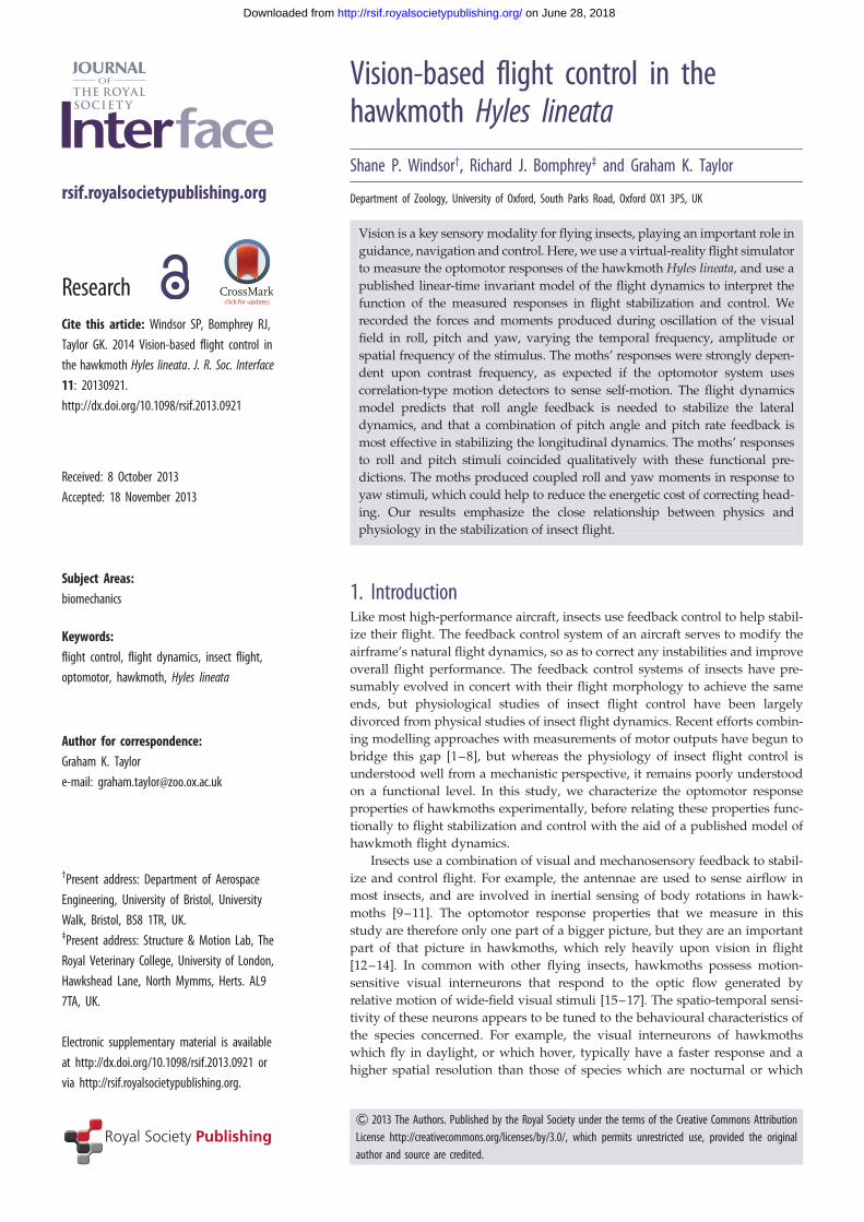
2.2. Experimental apparatusWe measured the forces and moments produced by H. lineata in

response to moving wide-field visual stimuli (figure 1a).

The moths were tethered to a six-component strain gauge

balance (Nano17, ATI Industrial Automation, NC, USA), with

constant voltage excitation provided by a signal conditioning

amplifier (2210A, Vishay, NC, USA). The amplified signals

were low-pass filtered at 1 kHz, and sampled at 10 kHz (Power-

Lab/16SP, ADInstruments, NSW, Australia). The moths were

mounted at the centre of a 1 m diameter hollow clear acrylic

sphere coated with rear-projection paint (Rear Projection

Screen Goo, Goo Systems, NV, USA). Two data projectors

with DC lamps (LT170, NEC, Japan) were retrofitted with

specialized micromirror chipsets (ALP-2, ViALUX, Chemnitz,

Germany), and used to project eight-bit greyscale 1024 � 768

pixel images at 144 Hz onto the surface of the sphere (see

§2.4 for details of stimulus design). The light levels inside the

sphere (80 lux) were similar to those which would be encoun-

tered by the moths around dusk. The moths were not

provided with any extrinsic airflow, but the flows induced by

their own wingbeat would have induced a significant airflow

stimulus over the antennae, as is known to be the case during

hovering [27].

2.3. Axis systemsWe used a right-handed axis system to define the moth’s

body axes, with the origin of the body axis system located

at the centre of mass of the moth. We resolved the forces

and moments in these body axes, and used the same set of

body axes to describe the visual stimuli that we presented.

The body axis system was oriented with its y-axis (i.e. pitch

axis) normal to the moth’s symmetry plane, and with its

x-axis (i.e. roll axis) and z-axis (i.e. yaw axis) fixed by aligning

the z-axis with the gravity vector when the moth was tethered

(figure 1b). The same body-fixed axis system was used when

modelling the flight dynamics, with the z-axis of the body

axes fixed so as to be aligned with the gravity vector at

equilibrium. For the purposes of the flight dynamics model-

ling, we used (u,v,w) and ( p,q,r) to represent the (x,y,z)

(a) (b) (c)

1

25

3

4

roll

pitch

yaw

6

40°

rotation axis

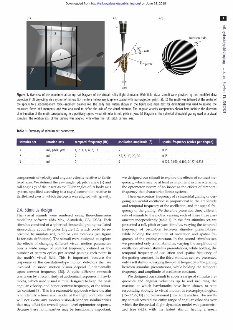
Figure 1. Overview of the experimental set-up. (a) Diagram of the virtual-reality flight simulator. Wide-field visual stimuli were provided by two modified dataprojectors (1,2) projecting via a system of mirrors (3,4), onto a hollow acrylic sphere coated with rear-projection paint (5). (b) The moth was tethered at the centre ofthe sphere to a six-component force – moment balance (6). The body axis system shown in the figure (see main text for definitions) was used to resolve themeasured forces and moments, and was also used to define the axis of the visual stimulus. The angular velocity components shown here indicate the directionof self-motion of the moth corresponding to a positively signed visual stimulus in roll, pitch or yaw. (c) Diagram of the spherical sinusoidal grating used as a visualstimulus. The rotation axis of the grating was aligned with either the roll, pitch or yaw axis.

Table 1. Summary of stimulus set parameters.

stimulus set rotation axis temporal frequency (Hz) oscillation amplitude (88888) spatial frequency (cycles per degree)

1 roll, pitch, yaw 1, 2, 3, 4, 6, 8, 12 5 0.05

2 roll 2 2.5, 5, 10, 20, 30 0.05

3 roll 2 5 0.025, 0.050, 0.100, 0.167, 0.333

rsif.royalsocietypublishing.orgJ.R.Soc.Interface

11:20130921

3

on June 28, 2018http://rsif.royalsocietypublishing.org/Downloaded from

components of velocity and angular velocity relative to Earth-

fixed axes. We defined the yaw angle (c), pitch angle (u) and

roll angle (g) of the insect as the Euler angles of its body axis

system, specified according to a (z,y,x) convention relative to

Earth-fixed axes in which the z-axis was aligned with gravity.

2.4. Stimulus designThe visual stimuli were rendered using three-dimension

modelling software (3ds Max, Autodesk, CA, USA). Each

stimulus consisted of a spherical sinusoidal grating oscillated

sinusoidally about its poles (figure 1c), which could be re-

oriented to simulate roll, pitch or yaw rotations (see figure

1b for axis definitions). The stimuli were designed to explore

the effects of changing different visual motion parameters

over a wide range of contrast frequency, defined as the

number of pattern cycles per second passing each point in

the moth’s visual field. This is important, because the

responses of the correlation-type motion detectors that are

involved in insect motion vision depend fundamentally

upon contrast frequency [28]. A quite different approach

was taken by a recent study of abdominal responses in hawk-

moths, which used visual stimuli designed to keep the peak

angular velocity, and hence contrast frequency, of the stimu-

lus constant [8]. This is a reasonable approach where the aim

is to identify a linearized model of the flight controller, but

will not excite any motion vision-dependent nonlinearities

that may affect the overall system-level optomotor response.

Because these nonlinearities may be functionally important,

we designed our stimuli to explore the effects of contrast fre-

quency, which may be at least as important in characterizing

the optomotor system of an insect as the effects of temporal

frequency that characterize linear systems.

The mean contrast frequency of a sinusoidal grating under-

going sinusoidal oscillation is proportional to the amplitude

and temporal frequency of the oscillation, and the spatial fre-

quency of the grating. We therefore presented three different

sets of stimuli to the moths, varying each of these three par-

ameters independently (table 1). In this first stimulus set, we

presented a roll, pitch or yaw stimulus, varying the temporal

frequency of oscillation between stimulus presentations,

while holding the amplitude of oscillation and spatial fre-

quency of the grating constant. In the second stimulus set,

we presented only a roll stimulus, varying the amplitude of

oscillation between stimulus presentations, while holding the

temporal frequency of oscillation and spatial frequency of

the grating constant. In the third stimulus set, we presented

only a roll stimulus, varying the spatial frequency of the grating

between stimulus presentations, while holding the temporal

frequency and amplitude of oscillation constant.

We designed our stimuli to cover a range of stimulus fre-

quencies and angular velocities up to and including the

maxima at which hawkmoths have been shown to stop

responding strongly to visual motion in electrophysiological

[15–17,29,30] and behavioural [12–14,31] studies. The result-

ing stimuli covered the entire range of angular velocities over

which the theoretical flight dynamics model was parametri-

zed (see §4.1), with the fastest stimuli having a mean

0

50

100

150

Mro

ll po

wer

N2

m2 s

10–1

2

0

20

40

60

80

stim

ulus

pow

erde

g2 s

0 5 10 15

0.5

1.0

cohe

renc

efrequency (Hz)

(a)

(b)

(c)

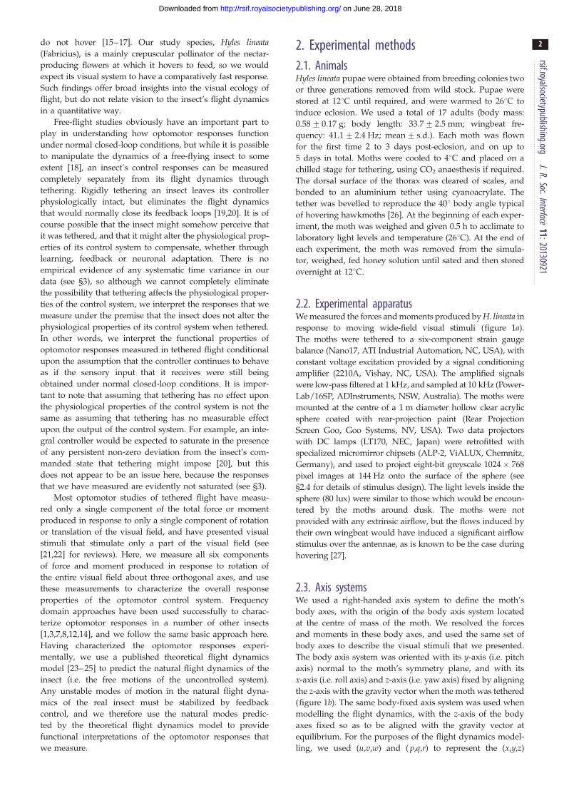
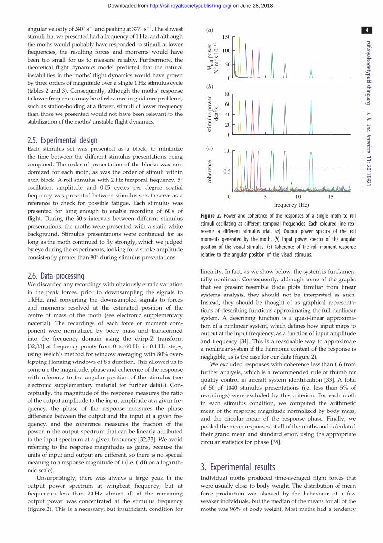
Figure 2. Power and coherence of the responses of a single moth to rollstimuli oscillating at different temporal frequencies. Each coloured line rep-resents a different stimulus trial. (a) Output power spectra of the rollmoments generated by the moth. (b) Input power spectra of the angularposition of the visual stimulus. (c) Coherence of the roll moment responserelative to the angular position of the visual stimulus.

rsif.royalsocietypublishing.orgJ.R.Soc.Interface

11:20130921

4

on June 28, 2018http://rsif.royalsocietypublishing.org/Downloaded from

angular velocity of 2408 s–1 and peaking at 3778 s–1. The slowest

stimuli that we presented had a frequency of 1 Hz, and although

the moths would probably have responded to stimuli at lower

frequencies, the resulting forces and moments would have

been too small for us to measure reliably. Furthermore, the

theoretical flight dynamics model predicted that the natural

instabilities in the moths’ flight dynamics would have grown

by three orders of magnitude over a single 1 Hz stimulus cycle

(tables 2 and 3). Consequently, although the moths’ response

to lower frequencies may be of relevance in guidance problems,

such as station-holding at a flower, stimuli of lower frequency

than those we presented would not have been relevant to the

stabilization of the moths’ unstable flight dynamics.

2.5. Experimental designEach stimulus set was presented as a block, to minimize

the time between the different stimulus presentations being

compared. The order of presentation of the blocks was ran-

domized for each moth, as was the order of stimuli within

each block. A roll stimulus with 2 Hz temporal frequency, 58oscillation amplitude and 0.05 cycles per degree spatial

frequency was presented between stimulus sets to serve as a

reference to check for possible fatigue. Each stimulus was

presented for long enough to enable recording of 60 s of

flight. During the 30 s intervals between different stimulus

presentations, the moths were presented with a static white

background. Stimulus presentations were continued for as

long as the moth continued to fly strongly, which we judged

by eye during the experiments, looking for a stroke amplitude

consistently greater than 908 during stimulus presentations.

2.6. Data processingWe discarded any recordings with obviously erratic variation

in the peak forces, prior to downsampling the signals to

1 kHz, and converting the downsampled signals to forces

and moments resolved at the estimated position of the

centre of mass of the moth (see electronic supplementary

material). The recordings of each force or moment com-

ponent were normalized by body mass and transformed

into the frequency domain using the chirp-Z transform

[32,33] at frequency points from 0 to 60 Hz in 0.1 Hz steps,

using Welch’s method for window averaging with 80% over-

lapping Hanning windows of 8 s duration. This allowed us to

compute the magnitude, phase and coherence of the response

with reference to the angular position of the stimulus (see

electronic supplementary material for further detail). Con-

ceptually, the magnitude of the response measures the ratio

of the output amplitude to the input amplitude at a given fre-

quency, the phase of the response measures the phase

difference between the output and the input at a given fre-

quency, and the coherence measures the fraction of the

power in the output spectrum that can be linearly attributed

to the input spectrum at a given frequency [32,33]. We avoid

referring to the response magnitudes as gains, because the

units of input and output are different, so there is no special

meaning to a response magnitude of 1 (i.e. 0 dB on a logarith-

mic scale).

Unsurprisingly, there was always a large peak in the

output power spectrum at wingbeat frequency, but at

frequencies less than 20 Hz almost all of the remaining

output power was concentrated at the stimulus frequency

(figure 2). This is a necessary, but insufficient, condition for

linearity. In fact, as we show below, the system is fundamen-

tally nonlinear. Consequently, although some of the graphs

that we present resemble Bode plots familiar from linear

systems analysis, they should not be interpreted as such.

Instead, they should be thought of as graphical representa-

tions of describing functions approximating the full nonlinear

system. A describing function is a quasi-linear approxima-

tion of a nonlinear system, which defines how input maps to

output at the input frequency, as a function of input amplitude

and frequency [34]. This is a reasonable way to approximate

a nonlinear system if the harmonic content of the response is

negligible, as is the case for our data (figure 2).

We excluded responses with coherence less than 0.6 from

further analysis, which is a recommended rule of thumb for

quality control in aircraft system identification [33]. A total

of 50 of 1040 stimulus presentations (i.e. less than 5% of

recordings) were excluded by this criterion. For each moth

in each stimulus condition, we computed the arithmetic

mean of the response magnitude normalized by body mass,

and the circular mean of the response phase. Finally, we

pooled the mean responses of all of the moths and calculated

their grand mean and standard error, using the appropriate

circular statistics for phase [35].

3. Experimental resultsIndividual moths produced time-averaged flight forces that

were usually close to body weight. The distribution of mean

force production was skewed by the behaviour of a few

weaker individuals, but the median of the means for all of the

moths was 96% of body weight. Most moths had a tendency

phas

e (°

) co

here

nce

frequency (Hz) frequency (Hz)20 40 80 120 240 20 40 80 120 240 20 40 80 120 240

frequency (Hz)mean angular velocity

(deg s–1)mean angular velocity

(deg s–1)mean angular velocity

(deg s–1)

(a)

(b)

(c)

(d)

(e)

( f )

(g)

(h)

(i)

0.3

0.5

1

234

mag

nitu

de

N m

kg–1

deg

–1 1

0–3

–360

–270

–180

–90

0

90

1 2 4 6 8 120.6

0.8

1 16 17 17 16 17 16 16

1 2 4 6 8 12

13 14 15 15 15 14 15

1 2 4 6 8 12

10 15 14 15 14 14 12

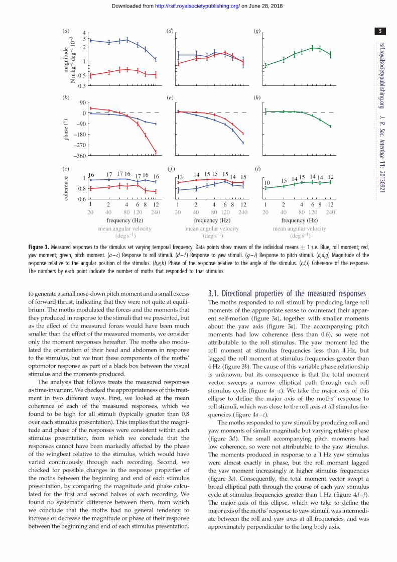
Figure 3. Measured responses to the stimulus set varying temporal frequency. Data points show means of the individual means+ 1 s.e. Blue, roll moment; red,yaw moment; green, pitch moment. (a – c) Response to roll stimuli. (d – f ) Response to yaw stimuli. (g – i) Response to pitch stimuli. (a,d,g) Magnitude of theresponse relative to the angular position of the stimulus. (b,e,h) Phase of the response relative to the angle of the stimulus. (c,f,i) Coherence of the response.The numbers by each point indicate the number of moths that responded to that stimulus.

rsif.royalsocietypublishing.orgJ.R.Soc.Interface

11:20130921

5

on June 28, 2018http://rsif.royalsocietypublishing.org/Downloaded from

to generate a small nose-down pitch moment and a small excess

of forward thrust, indicating that they were not quite at equili-

brium. The moths modulated the forces and the moments that

they produced in response to the stimuli that we presented, but

as the effect of the measured forces would have been much

smaller than the effect of the measured moments, we consider

only the moment responses hereafter. The moths also modu-

lated the orientation of their head and abdomen in response

to the stimulus, but we treat these components of the moths’

optomotor response as part of a black box between the visual

stimulus and the moments produced.

The analysis that follows treats the measured responses

as time-invariant. We checked the appropriateness of this treat-

ment in two different ways. First, we looked at the mean

coherence of each of the measured responses, which we

found to be high for all stimuli (typically greater than 0.8

over each stimulus presentation). This implies that the magni-

tude and phase of the responses were consistent within each

stimulus presentation, from which we conclude that the

responses cannot have been markedly affected by the phase

of the wingbeat relative to the stimulus, which would have

varied continuously through each recording. Second, we

checked for possible changes in the response properties of

the moths between the beginning and end of each stimulus

presentation, by comparing the magnitude and phase calcu-

lated for the first and second halves of each recording. We

found no systematic difference between them, from which

we conclude that the moths had no general tendency to

increase or decrease the magnitude or phase of their response

between the beginning and end of each stimulus presentation.

3.1. Directional properties of the measured responsesThe moths responded to roll stimuli by producing large roll

moments of the appropriate sense to counteract their appar-

ent self-motion (figure 3a), together with smaller moments

about the yaw axis (figure 3a). The accompanying pitch

moments had low coherence (less than 0.6), so were not

attributable to the roll stimulus. The yaw moment led the

roll moment at stimulus frequencies less than 4 Hz, but

lagged the roll moment at stimulus frequencies greater than

4 Hz (figure 3b). The cause of this variable phase relationship

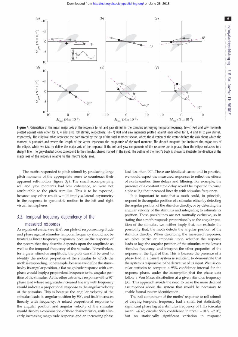
is unknown, but its consequence is that the total moment

vector sweeps a narrow elliptical path through each roll

stimulus cycle (figure 4a–c). We take the major axis of this

ellipse to define the major axis of the moths’ response to

roll stimuli, which was close to the roll axis at all stimulus fre-

quencies (figure 4a–c).

The moths responded to yaw stimuli by producing roll and

yaw moments of similar magnitude but varying relative phase

(figure 3d). The small accompanying pitch moments had

low coherence, so were not attributable to the yaw stimulus.

The moments produced in response to a 1 Hz yaw stimulus

were almost exactly in phase, but the roll moment lagged

the yaw moment increasingly at higher stimulus frequencies

(figure 3e). Consequently, the total moment vector swept a

broad elliptical path through the course of each yaw stimulus

cycle at stimulus frequencies greater than 1 Hz (figure 4d–f).The major axis of this ellipse, which we take to define the

major axis of the moths’ response to yaw stimuli, was intermedi-

ate between the roll and yaw axes at all frequencies, and was

approximately perpendicular to the long body axis.

–10

–5

0

5

10

–7°

Mya

w (

N m

10–6

)

(a)

–13°

(b)

8°

(c)

Mroll (N m 10–6)

Mya

w (

N m

10–6

)

(d)

–10 0 10

–10

–5

0

5

10

–34°

Mroll (N m 10–6)

(e)

–10 0 10

–40°

Mroll (N m 10–6)

( f )

–10 0 10

–49°

stim

ulus

angl

e

Figure 4. Orientation of the mean major axis of the response to roll and yaw stimuli in the stimulus set varying temporal frequency. (a – c) Roll and yaw momentsplotted against each other for 1, 4 and 8 Hz roll stimuli, respectively. (d – f ) Roll and yaw moments plotted against each other for 1, 4 and 8 Hz yaw stimuli,respectively. The elliptical orbits represent the path traced by the tip of the total moment vector, where the direction of the vector defines the axis about which themoment is produced and where the length of the vector represents the magnitude of the total moment. The dashed magenta line indicates the major axis ofthe ellipse, which we take to define the major axis of the response. If the roll and yaw components of the response are in phase, then the ellipse collapses to astraight line. The grey-shaded circles correspond to the stimulus phases marked in the inset. The outline of the moth’s body is shown to illustrate the direction of themajor axis of the response relative to the moth’s body axes.

rsif.royalsocietypublishing.orgJ.R.Soc.Interface

11:20130921

6

on June 28, 2018http://rsif.royalsocietypublishing.org/Downloaded from

The moths responded to pitch stimuli by producing large

pitch moments of the appropriate sense to counteract their

apparent self-motion (figure 3g). The small accompanying

roll and yaw moments had low coherence, so were not

attributable to the pitch stimulus. This is to be expected,

because any other result would imply a lateral asymmetry

in the response to symmetric motion in the left and right

visual hemispheres.

3.2. Temporal frequency dependency of themeasured responses

As explained earlier (see §2.6), our plots of response magnitude

and phase against stimulus temporal frequency should not be

treated as linear frequency responses, because the response of

the system that they describe depends upon the amplitude as

well as the temporal frequency of the stimulus. Nevertheless,

for a given stimulus amplitude, the plots can still be used to

identify the motion properties of the stimulus to which the

moth is responding. For example, because we define the stimu-

lus by its angular position, a flat magnitude response with zero

phase would imply a proportional response to the angular pos-

ition of the stimulus. At the other extreme, a response with a 908phase lead whose magnitude increased linearly with frequency

would indicate a proportional response to the angular velocity

of the stimulus. This is because the angular velocity of the

stimulus leads its angular position by 908, and itself increases

linearly with frequency. A mixed proportional response to

the angular position and angular velocity of the stimulus

would display a combination of these characteristics, with a lin-

early increasing magnitude response and an increasing phase

lead less than 908. These are idealized cases, and in practice,

we would expect the measured responses to reflect the effects

of nonlinearities, time delays and filtering. For example, the

presence of a constant time delay would be expected to cause

a phase lag that increased linearly with stimulus frequency.

It is important to note that a moth could, in principle,

respond to the angular position of a stimulus either by detecting

the angular position of the stimulus directly, or by detecting the

angular velocity of the stimulus and integrating to estimate its

position. These possibilities are not mutually exclusive, so in

stating that a moth responds proportionally to the angular pos-

ition of the stimulus, we neither imply that, nor exclude the

possibility that, the moth detects the angular position of the

stimulus directly. When describing the measured responses,

we place particular emphasis upon whether the response

leads or lags the angular position of the stimulus at the lowest

stimulus frequency, and interpret the other properties of the

response in the light of this. This is because the presence of a

phase lead in a causal system is sufficient to demonstrate that

the system is responsive to the derivative of its input. We use cir-

cular statistics to compute a 95% confidence interval for the

response phase, under the assumption that the phase data

follow a Von Mises distribution at a given stimulus frequency

[35]. This approach avoids the need to make the more detailed

assumptions about the system that would be necessary to

enable formal system identification.

The roll component of the moths’ response to roll stimuli

of varying temporal frequency had a small but statistically

significant phase lag at a stimulus frequency of 1 Hz (circular

mean: –6.48; circular 95% confidence interval: –10.8, –2.08),but no statistically significant variation in response

rsif.royalsocietypublishing.orgJ.R.Soc.Interface

11:20130921

7

on June 28, 2018http://rsif.royalsocietypublishing.org/Downloaded from

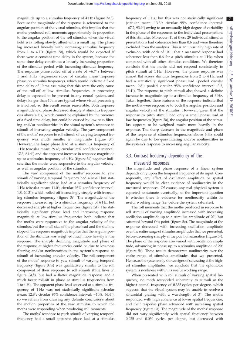
magnitude up to a stimulus frequency of 4 Hz (figure 3a,b).

Because the magnitude of the response is referenced to the

angular position of the visual stimulus, this implies that the

moths produced roll moments approximately in proportion

to the angular position of the roll stimulus when the visual

field was rolling slowly, albeit with a small lag. The phase

lag increased linearly with increasing stimulus frequency

from 1 to 4 Hz (figure 3b), which would be expected if

there were a constant time delay in the system, because the

same time delay constitutes a linearly increasing proportion

of the stimulus period with increasing stimulus frequency.

The response phase rolled off at a rate of –6.78 s between

1 and 4 Hz (regression slope of circular mean response

phase on stimulus frequency), which would indicate a fixed

time delay of 19 ms assuming that this were the only cause

of the roll-off at low stimulus frequencies. A processing

delay is expected to be present in any neural system, and

delays longer than 10 ms are typical where visual processing

is involved, so this result seems reasonable. Both response

magnitude and phase decreased sharply at stimulus frequen-

cies above 4 Hz, which cannot be explained by the presence

of a fixed time delay, but could be caused by low-pass filter-

ing and/or nonlinearities in the visual system’s response to

stimuli of increasing angular velocity. The yaw component

of the moths’ response to roll stimuli of varying temporal fre-

quency was much smaller in magnitude (figure 3a).

However, the large phase lead at a stimulus frequency of

1 Hz (circular mean: 39.48; circular 95% confidence interval:

17.3, 61.48) and the apparent increase in response magnitude

up to a stimulus frequency of 4 Hz (figure 3b) together indi-

cate that the moths were responsive to the angular velocity,

as well as angular position, of the stimulus.

The yaw component of the moths’ response to yaw

stimuli of varying temporal frequency had a small but stat-

istically significant phase lead at a stimulus frequency of

1 Hz (circular mean: 11.08; circular 95% confidence interval:

1.8, 20.38), which rolled off increasingly steeply with increas-

ing stimulus frequency (figure 3e). The magnitude of the

response increased up to a stimulus frequency of 6 Hz, but

decreased sharply at higher frequencies (figure 3d ). The stat-

istically significant phase lead and increasing response

magnitude at low-stimulus frequencies both indicate that

the moths were responsive to the angular velocity of the

stimulus, but the small size of the phase lead and the shallow

slope of the response magnitude implies that the angular pos-

ition of the stimulus was weighted much more heavily in the

response. The sharply declining magnitude and phase of

the response at higher frequencies could be due to low-pass

filtering and/or nonlinearities in the system’s response to

stimuli of increasing angular velocity. The roll component

of the moths’ response to yaw stimuli of varying temporal

frequency (figure 3d,e) was qualitatively similar to the roll

component of their response to roll stimuli (blue lines in

figure 3a,b), but had a flatter magnitude response and a

much faster roll-off in phase at stimulus frequencies from

1 to 4 Hz. The apparent phase lead observed at a stimulus fre-

quency of 1 Hz was not statistically significant (circular

mean: 12.88; circular 95% confidence interval: –10.8, 36.48),so we refrain from drawing any definite conclusions about

the motion properties of the yaw stimulus to which the

moths were responding when producing roll moments.

The moths’ response to pitch stimuli of varying temporal

frequency had a small apparent phase lead at a stimulus

frequency of 1 Hz, but this was not statistically significant

(circular mean: 13.38; circular 95% confidence interval:

–67.2, 93.98) owing to an unusually high degree of variability

in the phase of the responses to the individual presentations

of this stimulus. Moreover, 11 of these 29 individual stimulus

presentations had coherence less than 0.6 and were therefore

excluded from the analysis. This is an unusually high rate of

exclusion, with odds of 10 : 1 that a measured response had

coherence less than 0.6 for a pitch stimulus at 1 Hz, when

compared with all other stimulus conditions. We therefore

conclude that the moths did not respond consistently to

pitch stimuli at 1 Hz. However, the phase response was

almost flat across stimulus frequencies from 2 to 4 Hz, and

had a statistically significant phase lead (pooled circular

mean: 9.88; pooled circular 95% confidence interval: 3.2,

16.48). The response to pitch stimuli also showed a definite

increase in magnitude up to a stimulus frequency of 6 Hz.

Taken together, these features of the response indicate that

the moths were responsive to both the angular position and

angular velocity of the stimulus. However, given that the

response to pitch stimuli had only a small phase lead at

low frequencies (figure 3h), the angular position of the stimu-

lus appears to be weighted much more heavily in the

response. The sharp decrease in the magnitude and phase

of the response at stimulus frequencies above 6 Hz could

again be due to low-pass filtering and/or nonlinearities in

the system’s response to increasing angular velocity.

3.3. Contrast frequency dependency of themeasured responses

The magnitude and phase response of a linear system

depends only upon the temporal frequency of its input. Con-

sequently, any effect of oscillation amplitude or spatial

frequency would be clear evidence of nonlinearity in the

measured responses. Of course, any real physical system is

expected to saturate eventually, so the important question

is whether there is evidence for nonlinearity within its

useful working range (i.e. before the system saturates).

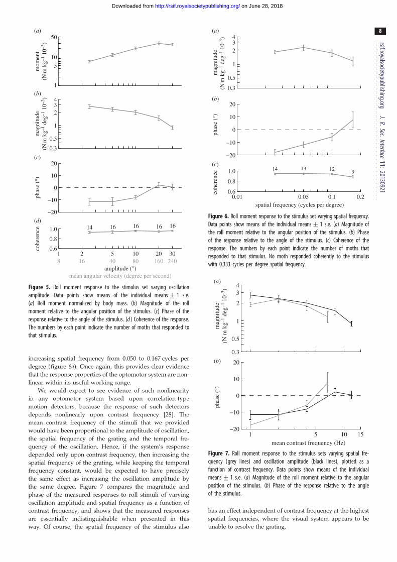
The roll moments that the moths produced in response to

roll stimuli of varying amplitude increased with increasing

oscillation amplitude up to a stimulus amplitude of 208, but

saturated beyond this point (figure 5a). The magnitude of the

response decreased with increasing oscillation amplitude

over the entire range of stimulus amplitudes that we presented,

before decreasing sharply at the point of saturation (figure 5b).

The phase of the response also varied with oscillation ampli-

tude, advancing in phase up to a stimulus amplitude of 208(figure 5c). These results demonstrate nonlinearity over the

entire range of stimulus amplitudes that we presented.

Hence, as the system only shows signs of saturating at the high-

est stimulus amplitudes, we conclude that the optomotor

system is nonlinear within its useful working range.

When presented with roll stimuli of varying spatial fre-

quency, no moth responded coherently to stimuli at the

highest spatial frequency of 0.333 cycles per degree, which

suggests that the visual system may be unable to resolve a

sinusoidal grating with a wavelength of 38. The moths

responded with high coherence at lower spatial frequencies,

and their response phase advanced with increasing spatial

frequency (figure 6b). The magnitude of the moths’ response

did not vary significantly with spatial frequency between

0.025 and 0.050 cycles per degree, but decreased with

mom

ent

(N m

kg–1

10–3

)

0.3

0.5

1

234

mag

nitu

de(N

m k

g–1 d

eg–1

10–3

)

–20

–10

0

10

20

phas

e (°

)

1 2 5 10 20 300.6

0.8

1.0 14 16 16 16 16

amplitude (°)

cohe

renc

e

1

5

10

50(a)

(b)

(c)

(d)

168 40 80 160 240

mean angular velocity (degree per second)

Figure 5. Roll moment response to the stimulus set varying oscillationamplitude. Data points show means of the individual means+ 1 s.e.(a) Roll moment normalized by body mass. (b) Magnitude of the rollmoment relative to the angular position of the stimulus. (c) Phase of theresponse relative to the angle of the stimulus. (d ) Coherence of the response.The numbers by each point indicate the number of moths that responded tothat stimulus.

−20

–10

0

10

20

phas

e (°

)

0.01 0.05 0.1 0.20.6

0.8

1.0 9121314

spatial frequency (cycles per degree)

cohe

renc

e

(a)

(b)

(c)

0.3

0.5

1

234

mag

nitu

de(N

m k

g–1 d

eg–1

10–3

) Figure 6. Roll moment response to the stimulus set varying spatial frequency.Data points show means of the individual means+ 1 s.e. (a) Magnitude ofthe roll moment relative to the angular position of the stimulus. (b) Phaseof the response relative to the angle of the stimulus. (c) Coherence of theresponse. The numbers by each point indicate the number of moths thatresponded to that stimulus. No moth responded coherently to the stimuluswith 0.333 cycles per degree spatial frequency.

phas

e (°

)

(a)

(b)

0.3

0.5

1

2

34

mag

nitu

de(N

m k

g–1 d

eg–1

10–3

)

1 5 10 15−20

−10

0

10

20

mean contrast frequency (Hz)

Figure 7. Roll moment response to the stimulus sets varying spatial fre-quency (grey lines) and oscillation amplitude (black lines), plotted as afunction of contrast frequency. Data points show means of the individualmeans+ 1 s.e. (a) Magnitude of the roll moment relative to the angularposition of the stimulus. (b) Phase of the response relative to the angleof the stimulus.

rsif.royalsocietypublishing.orgJ.R.Soc.Interface

11:20130921

8

on June 28, 2018http://rsif.royalsocietypublishing.org/Downloaded from

increasing spatial frequency from 0.050 to 0.167 cycles per

degree (figure 6a). Once again, this provides clear evidence

that the response properties of the optomotor system are non-

linear within its useful working range.

We would expect to see evidence of such nonlinearity

in any optomotor system based upon correlation-type

motion detectors, because the response of such detectors

depends nonlinearly upon contrast frequency [28]. The

mean contrast frequency of the stimuli that we provided

would have been proportional to the amplitude of oscillation,

the spatial frequency of the grating and the temporal fre-

quency of the oscillation. Hence, if the system’s response

depended only upon contrast frequency, then increasing the

spatial frequency of the grating, while keeping the temporal

frequency constant, would be expected to have precisely

the same effect as increasing the oscillation amplitude by

the same degree. Figure 7 compares the magnitude and

phase of the measured responses to roll stimuli of varying

oscillation amplitude and spatial frequency as a function of

contrast frequency, and shows that the measured responses

are essentially indistinguishable when presented in this

way. Of course, the spatial frequency of the stimulus also

has an effect independent of contrast frequency at the highest

spatial frequencies, where the visual system appears to be

unable to resolve the grating.

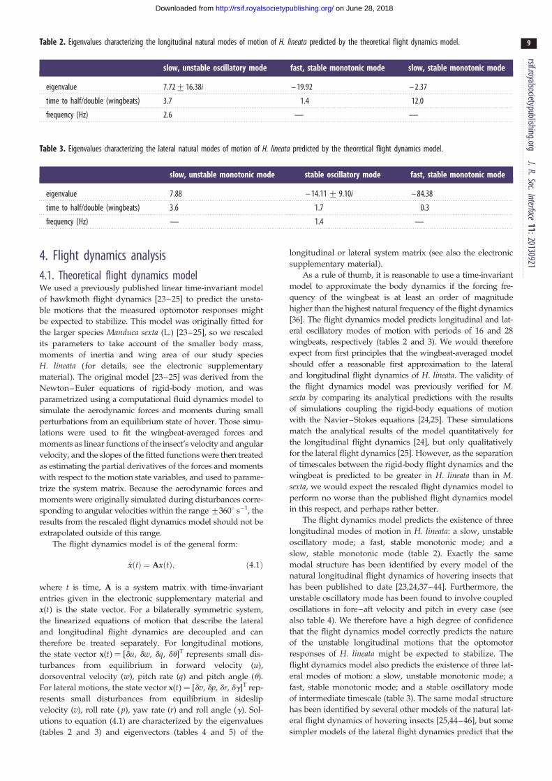
Table 3. Eigenvalues characterizing the lateral natural modes of motion of H. lineata predicted by the theoretical flight dynamics model.

slow, unstable monotonic mode stable oscillatory mode fast, stable monotonic mode

eigenvalue 7.88 – 14.11+ 9.10i – 84.38

time to half/double (wingbeats) 3.6 1.7 0.3

frequency (Hz) — 1.4 —

Table 2. Eigenvalues characterizing the longitudinal natural modes of motion of H. lineata predicted by the theoretical flight dynamics model.

slow, unstable oscillatory mode fast, stable monotonic mode slow, stable monotonic mode

eigenvalue 7.72+16.38i – 19.92 – 2.37

time to half/double (wingbeats) 3.7 1.4 12.0

frequency (Hz) 2.6 — —

rsif.royalsocietypublishing.orgJ.R.Soc.Interface

11:20130921

9

on June 28, 2018http://rsif.royalsocietypublishing.org/Downloaded from

4. Flight dynamics analysis4.1. Theoretical flight dynamics modelWe used a previously published linear time-invariant model

of hawkmoth flight dynamics [23–25] to predict the unsta-

ble motions that the measured optomotor responses might

be expected to stabilize. This model was originally fitted for

the larger species Manduca sexta (L.) [23–25], so we rescaled

its parameters to take account of the smaller body mass,

moments of inertia and wing area of our study species

H. lineata (for details, see the electronic supplementary

material). The original model [23–25] was derived from the

Newton–Euler equations of rigid-body motion, and was

parametrized using a computational fluid dynamics model to

simulate the aerodynamic forces and moments during small

perturbations from an equilibrium state of hover. Those simu-

lations were used to fit the wingbeat-averaged forces and

moments as linear functions of the insect’s velocity and angular

velocity, and the slopes of the fitted functions were then treated

as estimating the partial derivatives of the forces and moments

with respect to the motion state variables, and used to parame-

trize the system matrix. Because the aerodynamic forces and

moments were originally simulated during disturbances corre-

sponding to angular velocities within the range +3608 s–1, the

results from the rescaled flight dynamics model should not be

extrapolated outside of this range.

The flight dynamics model is of the general form:

_xðtÞ ¼ AxðtÞ; ð4:1Þ

where t is time, A is a system matrix with time-invariant

entries given in the electronic supplementary material and

x(t) is the state vector. For a bilaterally symmetric system,

the linearized equations of motion that describe the lateral

and longitudinal flight dynamics are decoupled and can

therefore be treated separately. For longitudinal motions,

the state vector x(t) ¼ [du, dw, dq, du]T represents small dis-

turbances from equilibrium in forward velocity (u),

dorsoventral velocity (w), pitch rate (q) and pitch angle (u).

For lateral motions, the state vector x(t) ¼ [dv, dp, dr, dg]T rep-

resents small disturbances from equilibrium in sideslip

velocity (v), roll rate ( p), yaw rate (r) and roll angle (g). Sol-

utions to equation (4.1) are characterized by the eigenvalues

(tables 2 and 3) and eigenvectors (tables 4 and 5) of the

longitudinal or lateral system matrix (see also the electronic

supplementary material).

As a rule of thumb, it is reasonable to use a time-invariant

model to approximate the body dynamics if the forcing fre-

quency of the wingbeat is at least an order of magnitude

higher than the highest natural frequency of the flight dynamics

[36]. The flight dynamics model predicts longitudinal and lat-

eral oscillatory modes of motion with periods of 16 and 28

wingbeats, respectively (tables 2 and 3). We would therefore

expect from first principles that the wingbeat-averaged model

should offer a reasonable first approximation to the lateral

and longitudinal flight dynamics of H. lineata. The validity of

the flight dynamics model was previously verified for M.sexta by comparing its analytical predictions with the results

of simulations coupling the rigid-body equations of motion

with the Navier–Stokes equations [24,25]. These simulations

match the analytical results of the model quantitatively for

the longitudinal flight dynamics [24], but only qualitatively

for the lateral flight dynamics [25]. However, as the separation

of timescales between the rigid-body flight dynamics and the

wingbeat is predicted to be greater in H. lineata than in M.sexta, we would expect the rescaled flight dynamics model to

perform no worse than the published flight dynamics model

in this respect, and perhaps rather better.

The flight dynamics model predicts the existence of three

longitudinal modes of motion in H. lineata: a slow, unstable

oscillatory mode; a fast, stable monotonic mode; and a

slow, stable monotonic mode (table 2). Exactly the same

modal structure has been identified by every model of the

natural longitudinal flight dynamics of hovering insects that

has been published to date [23,24,37–44]. Furthermore, the

unstable oscillatory mode has been found to involve coupled

oscillations in fore–aft velocity and pitch in every case (see

also table 4). We therefore have a high degree of confidence

that the flight dynamics model correctly predicts the nature

of the unstable longitudinal motions that the optomotor

responses of H. lineata might be expected to stabilize. The

flight dynamics model also predicts the existence of three lat-

eral modes of motion: a slow, unstable monotonic mode; a

fast, stable monotonic mode; and a stable oscillatory mode

of intermediate timescale (table 3). The same modal structure

has been identified by several other models of the natural lat-

eral flight dynamics of hovering insects [25,44–46], but some

simpler models of the lateral flight dynamics predict that the

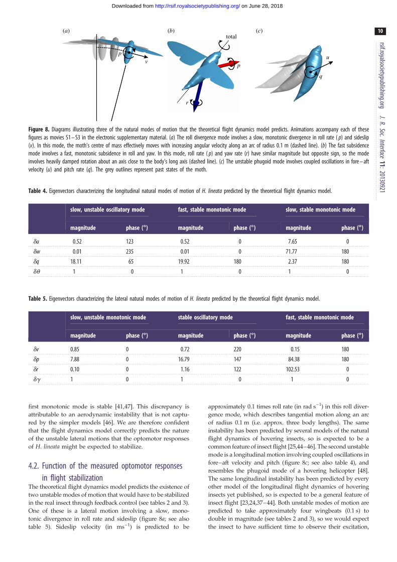
vu

q

p

(a) (b) (c)

p

total

r

Figure 8. Diagrams illustrating three of the natural modes of motion that the theoretical flight dynamics model predicts. Animations accompany each of thesefigures as movies S1 – S3 in the electronic supplementary material. (a) The roll divergence mode involves a slow, monotonic divergence in roll rate ( p) and sideslip(v). In this mode, the moth’s centre of mass effectively moves with increasing angular velocity along an arc of radius 0.1 m (dashed line). (b) The fast subsidencemode involves a fast, monotonic subsidence in roll and yaw. In this mode, roll rate ( p) and yaw rate (r) have similar magnitude but opposite sign, so the modeinvolves heavily damped rotation about an axis close to the body’s long axis (dashed line). (c) The unstable phugoid mode involves coupled oscillations in fore – aftvelocity (u) and pitch rate (q). The grey outlines represent past states of the moth.

Table 4. Eigenvectors characterizing the longitudinal natural modes of motion of H. lineata predicted by the theoretical flight dynamics model.

slow, unstable oscillatory mode fast, stable monotonic mode slow, stable monotonic mode

magnitude phase (88888) magnitude phase (88888) magnitude phase (88888)

du 0.52 123 0.52 0 7.65 0

dw 0.01 235 0.01 0 71.77 180

dq 18.11 65 19.92 180 2.37 180

du 1 0 1 0 1 0

Table 5. Eigenvectors characterizing the lateral natural modes of motion of H. lineata predicted by the theoretical flight dynamics model.

slow, unstable monotonic mode stable oscillatory mode fast, stable monotonic mode

magnitude phase (88888) magnitude phase (88888) magnitude phase (88888)

dv 0.85 0 0.72 220 0.15 180

dp 7.88 0 16.79 147 84.38 180

dr 0.10 0 1.16 122 102.53 0

dg 1 0 1 0 1 0

rsif.royalsocietypublishing.orgJ.R.Soc.Interface

11:20130921

10

on June 28, 2018http://rsif.royalsocietypublishing.org/Downloaded from

first monotonic mode is stable [41,47]. This discrepancy is

attributable to an aerodynamic instability that is not captu-

red by the simpler models [46]. We are therefore confident

that the flight dynamics model correctly predicts the nature

of the unstable lateral motions that the optomotor responses

of H. lineata might be expected to stabilize.

4.2. Function of the measured optomotor responsesin flight stabilization

The theoretical flight dynamics model predicts the existence of

two unstable modes of motion that would have to be stabilized

in the real insect through feedback control (see tables 2 and 3).

One of these is a lateral motion involving a slow, mono-

tonic divergence in roll rate and sideslip (figure 8a; see also

table 5). Sideslip velocity (in ms–1) is predicted to be

approximately 0.1 times roll rate (in rad s–1) in this roll diver-

gence mode, which describes tangential motion along an arc

of radius 0.1 m (i.e. approx. three body lengths). The same

instability has been predicted by several models of the natural

flight dynamics of hovering insects, so is expected to be a

common feature of insect flight [25,44–46]. The second unstable

mode is a longitudinal motion involving coupled oscillations in

fore–aft velocity and pitch (figure 8c; see also table 4), and

resembles the phugoid mode of a hovering helicopter [48].

The same longitudinal instability has been predicted by every

other model of the longitudinal flight dynamics of hovering

insects yet published, so is expected to be a general feature of

insect flight [23,24,37–44]. Both unstable modes of motion are

predicted to take approximately four wingbeats (0.1 s) to

double in magnitude (see tables 2 and 3), so we would expect

the insect to have sufficient time to observe their excitation,

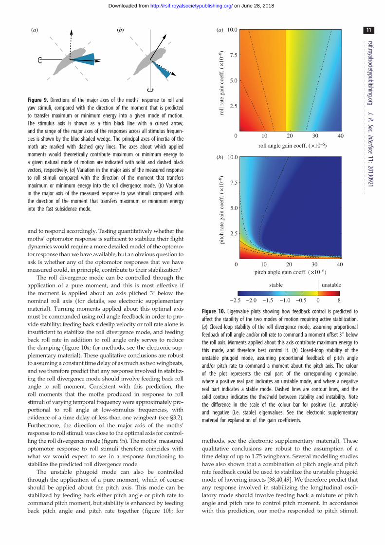
(a) (b)

Figure 9. Directions of the major axes of the moths’ response to roll andyaw stimuli, compared with the direction of the moment that is predictedto transfer maximum or minimum energy into a given mode of motion.The stimulus axis is shown as a thin black line with a curved arrow,and the range of the major axes of the responses across all stimulus frequen-cies is shown by the blue-shaded wedge. The principal axes of inertia of themoth are marked with dashed grey lines. The axes about which appliedmoments would theoretically contribute maximum or minimum energy toa given natural mode of motion are indicated with solid and dashed blackvectors, respectively. (a) Variation in the major axis of the measured responseto roll stimuli compared with the direction of the moment that transfersmaximum or minimum energy into the roll divergence mode. (b) Variationin the major axis of the measured response to yaw stimuli compared withthe direction of the moment that transfers maximum or minimum energyinto the fast subsidence mode.

stable unstable

−2.5 −2.0 −1.5 −1.0 −0.5 0 8

roll angle gain coeff. ( ×10–6)

(a)

10 20 30 400

2.5

5.0

7.5

10.0

(b)

10 20 30 400

2.5

5.0

7.5

10.0

roll

rate

gai

n co

eff.

(×

10–6

)pi

tch

rate

gai

n co

eff.

(×

10–6

)

pitch angle gain coeff. ( ×10–6)

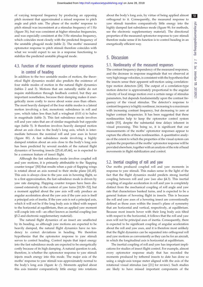
Figure 10. Eigenvalue plots showing how feedback control is predicted toaffect the stability of the two modes of motion requiring active stabilization.(a) Closed-loop stability of the roll divergence mode, assuming proportionalfeedback of roll angle and/or roll rate to command a moment offset 38 belowthe roll axis. Moments applied about this axis contribute maximum energy tothis mode, and therefore best control it. (b) Closed-loop stability of theunstable phugoid mode, assuming proportional feedback of pitch angleand/or pitch rate to command a moment about the pitch axis. The colourof the plot represents the real part of the corresponding eigenvalue,where a positive real part indicates an unstable mode, and where a negativereal part indicates a stable mode. Dashed lines are contour lines, and thesolid contour indicates the threshold between stability and instability. Notethe difference in the scale of the colour bar for positive (i.e. unstable)and negative (i.e. stable) eigenvalues. See the electronic supplementarymaterial for explanation of the gain coefficients.

rsif.royalsocietypublishing.orgJ.R.Soc.Interface

11:20130921

11

on June 28, 2018http://rsif.royalsocietypublishing.org/Downloaded from

and to respond accordingly. Testing quantitatively whether the

moths’ optomotor response is sufficient to stabilize their flight

dynamics would require a more detailed model of the optomo-

tor response than we have available, but an obvious question to

ask is whether any of the optomotor responses that we have

measured could, in principle, contribute to their stabilization?

The roll divergence mode can be controlled through the

application of a pure moment, and this is most effective if

the moment is applied about an axis pitched 38 below the

nominal roll axis (for details, see electronic supplementary

material). Turning moments applied about this optimal axis

must be commanded using roll angle feedback in order to pro-

vide stability: feeding back sideslip velocity or roll rate alone is

insufficient to stabilize the roll divergence mode, and feeding

back roll rate in addition to roll angle only serves to reduce

the damping (figure 10a; for methods, see the electronic sup-

plementary material). These qualitative conclusions are robust

to assuming a constant time delay of as much as two wingbeats,

and we therefore predict that any response involved in stabiliz-

ing the roll divergence mode should involve feeding back roll

angle to roll moment. Consistent with this prediction, the

roll moments that the moths produced in response to roll

stimuli of varying temporal frequency were approximately pro-

portional to roll angle at low-stimulus frequencies, with

evidence of a time delay of less than one wingbeat (see §3.2).

Furthermore, the direction of the major axis of the moths’

response to roll stimuli was close to the optimal axis for control-

ling the roll divergence mode (figure 9a). The moths’ measured

optomotor response to roll stimuli therefore coincides with

what we would expect to see in a response functioning to

stabilize the predicted roll divergence mode.

The unstable phugoid mode can also be controlled

through the application of a pure moment, which of course

should be applied about the pitch axis. This mode can be

stabilized by feeding back either pitch angle or pitch rate to

command pitch moment, but stability is enhanced by feeding

back pitch angle and pitch rate together (figure 10b; for

methods, see the electronic supplementary material). These

qualitative conclusions are robust to the assumption of a

time delay of up to 1.75 wingbeats. Several modelling studies

have also shown that a combination of pitch angle and pitch

rate feedback could be used to stabilize the unstable phugoid

mode of hovering insects [38,40,49]. We therefore predict that

any response involved in stabilizing the longitudinal oscil-

latory mode should involve feeding back a mixture of pitch

angle and pitch rate to control pitch moment. In accordance

with this prediction, our moths responded to pitch stimuli

rsif.royalsocietypublishing.orgJ.R.Soc.Interface

11:20130921

12

on June 28, 2018http://rsif.royalsocietypublishing.org/Downloaded from

of varying temporal frequency by producing an opposing

pitch moment that approximated a mixed response to pitch

angle and pitch rate. The phase of the moths’ response to

pitch stimuli was inconsistent at a stimulus frequency of 1 Hz

(figure 3h), but was consistent at higher stimulus frequencies,

and was especially consistent at the 3 Hz stimulus frequency,

which coincides most closely with the predicted frequency of

the unstable phugoid mode (table 2). The moths’ measured

optomotor response to pitch stimuli therefore coincides with

what we would expect to see in a response functioning to

stabilize the predicted unstable phugoid mode.

4.3. Function of the measured optomotor responsesin control of heading

In addition to the two unstable modes of motion, the theor-

etical flight dynamics model also predicts the existence of

four stable modes of motion in the natural flight dynamics

(tables 2 and 3). Motions that are naturally stable do not

require stabilization through feedback control, but they are

important nonetheless, because their damping makes it ener-

getically more costly to move about some axes than others.

The most heavily damped of the four stable modes is a lateral

motion involving a fast, monotonic subsidence in roll and

yaw, which takes less than half a wingbeat (0.01 s) to halve

in magnitude (table 3). This fast subsidence mode involves

roll and yaw rates that are of similar magnitude but opposite

sign (table 5). It therefore involves heavily damped motion

about an axis close to the body’s long axis, which is inter-

mediate between the nominal roll and yaw axes in hover

(figure 8b). A fast subsidence mode involving a highly

damped rotation about an axis close to the body’s long axis

has been predicted by several models of the natural flight

dynamics of hovering insects [25,41,45,46], so is expected to

be a common feature of insect flight.

Although the fast subsidence mode involves coupled roll

and yaw motions, it is primarily attributable to the ‘flapping

counter torque’ [50] that results when a pair of flapping wings

is rotated about an axis normal to their stroke plane [41,45].

This axis is always close to the yaw axis in hovering flight, so

to a first approximation, the fast subsidence mode is driven by

yaw rate damping. Flapping counter torques have been dis-

cussed extensively in the context of yaw turns [18,50–52], but

a moment applied about the yaw axis will only produce an

angular acceleration about the yaw axis if the yaw axis is itself

a principal axis of inertia. If the yaw axis is not a principal axis,

which it will not be if the long body axis is tilted with respect

to the horizontal at equilibrium, then an applied yaw moment

will couple into roll—an effect known as inertial coupling (see

§5.2 and electronic supplementary material).

The natural flight dynamics of an insect are unaffected

by its heading, so although yaw motions are expected to be

heavily damped, the natural flight dynamics have no ten-

dency to correct deviations in heading. We therefore

hypothesize that the optomotor response to yaw stimuli

serves to control heading. Control inputs that inject energy

into the fast subsidence mode are expected to be energetically

costly because of its high damping. A natural question to ask,

therefore, is whether the optomotor response to yaw stimuli

injects much energy into this mode. The major axis of the

moths’ response to yaw stimuli was approximately normal to

the body’s long axis (figure 4e–f ). Moments applied about

this axis transfer comparatively little energy into rotations

about the body’s long axis, by virtue of being applied almost

orthogonal to it. Consequently, the measured response to

yaw stimuli transfers comparatively little energy into the

highly damped fast subsidence mode (figure 9b; for methods,

see the electronic supplementary material). The directional

properties of the measured optomotor response to yaw stimuli

therefore make sense if its function is to control heading in an

energetically efficient way.

5. Discussion5.1. Nonlinearity of the measured responsesThe contrast frequency dependency of the measured responses,

and the decrease in response magnitude that we observed at

very high image velocities, is consistent with the hypothesis that

the insects sense their apparent self-motion using correlation-

type motion detectors [28]. The output of a correlation-type

motion detector is approximately proportional to the angular

velocity of local image motion over a certain range of stimulus

parameters, but depends fundamentally upon the contrast fre-

quency of the visual stimulus. The detector’s response to

contrast frequency is highly nonlinear, increasing to a maximum

with increasing contrast frequency, but decreasing to zero at

higher contrast frequencies. It has been suggested that these

nonlinearities help to keep the optomotor control system

stable [53], despite the substantial time delays inherent in

visual processing. This being so, it is significant that our

measurements of the moths’ optomotor responses appear to

capture the effects of these nonlinearities. A quantitative analy-

sis of the extent to which the properties of the visual system can

explain the properties of the moths’ optomotor response will be

provided elsewhere, together with an analysis of the role of head

movements in flight stabilization and control.

5.2. Inertial coupling of roll and yawOur moths produced coupled roll and yaw moments in

response to yaw stimuli. This makes sense in the light of the

fact that the flight dynamics model predicts strong inertial

coupling between roll and yaw (see also §4.3). This inertial

coupling of angular acceleration in roll and yaw is completely

distinct from the mechanical coupling of roll angle and yaw

rate that characterizes banked turns, and is expected to be a

general feature of hovering flight in insects. This is because

the roll and yaw axes of a hovering insect are conventionally

defined as those axes within the insect’s plane of symmetry

that are horizontal and vertical, respectively, at equilibrium.

Because most insects hover with their long body axis tilted

with respect to the horizontal, it follows that the roll and yaw

axes will not be principal axes of inertia. Consequently, there

is expected to be significant coupling of angular acceleration

about the roll and yaw axes, and it is therefore most unlikely

that the flight dynamics can be separated into orthogonal roll

and yaw motions as conveniently as they can be for an aircraft,

in which the longitudinal axis is horizontal at equilibrium.

The inertial coupling of roll and yaw has important impli-

cations for studies of insect flight control. For example, almost

every optomotor response study that has recorded the

moments produced by tethered insects to date has done so

using a single-axis torque meter aligned with the axis of the

rotational visual stimulus (see [21] for review). Such studies

are likely to have missed important components of the

rsif.royalsocietypublishing.orgJ.R.Soc.Interface

11:20130921

13

on June 28, 2018http://rsif.royalsocietypublishing.org/Downloaded from

optomotor response—especially in respect of yaw stimuli,

which we have shown elicit roll and yaw moments of similar

magnitude in hawkmoths. In a similar vein, several recent

studies of turning flight have treated free-flying insects as if

they were constrained to rotate about only the yaw axis

[18,50–52,54]. This treatment makes sense only if the yaw

axis is a principal axis of the body, and does not fully account

for the insect’s inertial properties if it is not.

5.3. Wider implicationsOur results show how the physiological responses of insects

can be related to the physics of their natural flight dynamics.

We have shown by example how a theoretical flight dynamics

model can be used to make detailed predictions about the

natural flight dynamics of an insect. The model predicts

the existence of two unstable modes of motion in the flight

dynamics of the uncontrolled system, so if the same instabilities

are present in the natural flight dynamics of the real insect, then

they must necessarily be stabilized through feedback control.

The model predicts that roll angle feedback without roll rate

feedback is appropriate to stabilize the lateral flight dynamics

through the application of a roll moment, but that a combi-

nation of pitch angle and pitch rate feedback will be most

effective in stabilizing the longitudinal flight dynamics

through the application of a pitch moment. The optomotor

responses that we have measured involve feeding back roll

angle to roll moment, and feeding back pitch angle and pitch

rate to pitch moment. The measured optomotor respon-

ses therefore coincide qualitatively with the control responses

that we would expect to see in a control system functioning

to stabilize the unstable modes of motion whose existence is

predicted by the theoretical flight dynamics model. Further-

more, the response properties that we have measured match

qualitatively those that would be expected given the known

properties of the interneurons that are responsible for proces-

sing motion vision. Our conclusions are therefore consistent

with the broader hypothesis that the sensorimotor systems of

insects are matched directly to the modes of motion that they

control [22]. Future work will test this mode-sensing hypo-

thesis directly by designing the visual stimuli that we present

to coincide with the non-orthogonal directions that we predict

are most relevant to the flight dynamics.

Acknowledgements. We thank Tony Price and John Hogg for technicalsupport in building the simulator and Rafał Zbikowski for manyhelpful discussions.

Funding statement. The research leading to these results has receivedfunding from the European Research Council under the EuropeanCommunity’s Seventh Framework Programme (FP7/2007-2013)/ERC grant agreement no. 204513. The virtual-reality flight simula-tor was built under BBSRC Research grant no. BBC5185731. R.J.B.is supported by EPSRC Fellowship EP/H004025/1.

References

1. Tanaka K, Kawachi K. 2006 Response characteristicsof visual altitude control system in Bombusterrestris. J. Exp. Biol. 209, 4533 – 4545.(doi:10.1242/jeb.02552)

2. Fry SN, Rohrseitz N, Straw AD, Dickinson MH. 2009Visual control of flight speed in Drosophilamelanogaster. J. Exp. Biol. 212, 1120 – 1130.(doi:10.1242/jeb.020768)

3. Graetzel CF, Nelson BJ, Fry SN. 2010 Frequencyresponse of lift control in Drosophila. J. R. Soc.Interface 7, 1603 – 1616. (doi:10.1098/rsif.2010.0040)

4. Straw AD, Lee S, Dickinson MH. 2010 Visualcontrol of altitude in flying Drosophila.Curr. Biol. 20, 1550 – 1556. (doi:10.1016/j.cub.2010.07.025)

5. Theobald JC, Ringach DL, Frye MA. 2010 Dynamicsof optomotor responses in Drosophila toperturbations in optic flow. J. Exp. Biol. 213,1366 – 1375. (doi:10.1242/jeb.037945)

6. Rohrseitz N, Fry SN. 2011 Behavioural systemidentification of visual flight speed control inDrosophila melanogaster. J. R. Soc. Interface 8,171 – 185. (doi:10.1098/rsif.2010.0225)

7. Roth E, Reiser MB, Dickinson MH, Cowan NJ. 2012 Atask-level model for optomotor yaw regulation inDrosophila melanogaster: a frequency-domain systemidentification approach. In IEEE 51st Annu. Conf. onDecision and Control (CDC), 10-13 December 2012,Maui, HI. IEEE. pp. 3721 – 3726.

8. Dyhr JP, Morgansen KA, Daniel TL, Cowan NJ. 2013Flexible strategies for flight control: an active role

for the abdomen. J. Exp. Biol. 216, 1523 – 1536.(doi:10.1242/jeb.077644)

9. Sane SP, Dieudonne A, Willis MA, Daniel TL. 2007Antennal mechanosensors mediate flight control inmoths. Science 315, 863 – 866. (doi:10.1126/science.1133598)

10. Hinterwirth AJ, Daniel TL. 2010 Antennae in thehawkmoth Manduca sexta (Lepidoptera,Sphingidae) mediate abdominal flexion in responseto mechanical stimuli. J. Comp. Physiol. A 196,947 – 956. (doi:10.1007/s00359-010-0578-5)

11. Hinterwirth AJ, Medina B, Lockey J, Otten D, VoldmanJ, Lang JH, Hildebrand JG, Daniel TL. 2012 Wirelessstimulation of antennal muscles in freely flyinghawkmoths leads to flight path changes. PLoS ONE 7,e52725. (doi:10.1371/journal.pone.0052725)

12. Farina WM, Varju D, Zhou Y. 1994 The regulation ofdistance to dummy flowers during hovering flight inthe hawk moth Macroglossum stellatarum. J. Comp.Physiol. A 174, 239 – 247. (doi:10.1007/BF00193790)

13. Farina WM, Kramer D, Varju D. 1995 The response ofthe hovering hawk moth Macroglossum stellatarumto translatory pattern motion. J. Comp. Physiol. A176, 551 – 562. (doi:10.1007/BF00196420)

14. Kern R, Varju D. 1998 Visual position stabilizationin the hummingbird hawk moth, Macroglossumstellatarum L. I. Behavioural analysis. J. Comp.Physiol. A 182, 225 – 237. (doi:10.1007/s003590050173)

15. O’Carroll DC, Bidwell NJ, Laughlin SB, Warrant EJ.1996 Insect motion detectors matched to visual

ecology. Nature 382, 63 – 66. (doi:10.1038/382063a0)

16. O’Carroll DC, Laughlin SB, Bidwell NJ, Harris RA. 1997Spatio-temporal properties of motion detectorsmatched to low image velocities in hovering insects.Vision Res. 37, 3427 – 3439. (doi:10.1016/S0042-6989(97) 00170-3)

17. Theobald JC, Warrant EJ, O’Carroll DC. 2010 Wide-field motion tuning in nocturnal hawkmoths.Proc. R. Soc. B 277, 853 – 860. (doi:10.1098/rspb.2009.1677)

18. Ristroph L, Bergou AJ, Ristroph G, Coumes K,Berman GJ, Guckenheimer J, Wang ZJ, Cohen I.2010 Discovering the flight autostabilizer of fruitflies by inducing aerial stumbles. Proc. Natl Acad.Sci. USA 107, 4820 – 4824. (doi:10.1073/pnas.1000615107)

19. Taylor GK, Zbikowski R. 2005 Nonlinear time-periodic models of the longitudinal flightdynamics of desert locusts Schistocerca gregaria.J. R. Soc. Interface 2, 197 – 221. (doi:10.1098/rsif.2005.0036)

20. Taylor GK, Bacic M, Bomphrey RJ, Carruthers AC,Gillies J, Walker SM, Thomas ALR. 2008 Newexperimental approaches to the biology of flightcontrol systems. J. Exp. Biol. 211, 258 – 266.(doi:10.1242/jeb.012625)

21. Taylor GK. 2001 Mechanics and aerodynamics ofinsect flight control. Biol. Rev. 76, 449 – 471.(doi:10.1017/S1464793101005759)

22. Taylor GK, Krapp HG. 2007 Sensory systems andflight stability: what do insects measure and why?

rsif.royalsocietypublishing.orgJ.R.Soc.Interface

11:20130921

14

on June 28, 2018http://rsif.royalsocietypublishing.org/Downloaded from

In Advances in insect physiology: insect mechanicsand control (eds J Casas, S Simpson), volume 34 ofAdvances in Insect Physiology, pp. 231 – 316.London, UK: Elsevier Academic Press.

23. Sun M, Wang J, Xiong Y. 2007 Dynamic flightstability of hovering insects. Acta Mech. Sin. 23,231 – 246. (doi:10.1007/s10409-007-0068-3)

24. Zhang Y-L, Sun M. 2010 Dynamic flight stability ofhovering model insects: theory versus simulationusing equations of motion coupled with Navier –Stokes equations. Acta Mech. Sin. 26, 509 – 520.(doi:10.1007/s10409-010-0360-5)

25. Zhang Y-L, Wu J-H, Sun M. 2012 Lateral dynamicflight stability of hovering insects: theory vs.numerical simulation. Acta Mech. Sin. 28, 221 – 231.(doi:10.1007/s10409-012-0011-0)

26. Willmott AP, Ellington CP. 1997 The mechanics offlight in the hawkmoth Manduca sexta.I. Kinematics of hovering and forward flight. J. Exp.Biol. 200, 2705 – 2722.

27. Sane SP, Jacobson NP. 2006 Induced airflow inflying insects II. Measurement of inducedflow. J. Exp. Biol. 209, 43 – 56. (doi:10.1242/jeb.01958)

28. Reichardt W. 1987 Evaluation of optical motioninformation by movement detectors. J. Comp.Physiol. 161, 533 – 547. (doi:10.1007/BF00603660)

29. Kern R. 1998 Visual position stabilization in thehummingbird hawk moth, Macroglossumstellatarum L. II. Electrophysiological analysis ofneurons sensitive to wide-field image motion.J. Comp. Physiol. A 182, 239 – 249. (doi:10.1007/s003590050174)

30. Sprayberry JDH. 2009 Responses of descendingvisually-sensitive neurons in the hawkmoth,Manduca sexta, to three-dimensional flower-likestimuli. J. Insect Sci. 9: 7. (doi:10.1673/031.009.0701)

31. Sprayberry JDH, Daniel TL. 2007 Flower tracking inhawkmoths: behavior and energetics. J. Exp. Biol.210, 37 – 45. (doi:10.1242/jeb.02616)

32. Bendat JS, Piersol AG. 1993 Engineering applications ofcorrelation and spectral analysis. New York, NY: Wiley.

33. Tischler MB, Remple RK. 2006 Aircraft and rotorcraftsystem identification: engineering methods withflight-test examples. Reston, VA: American Instituteof Aeronautics and Astronautics.

34. Slotine JJ, Wilson EL. 1991 Applied nonlinear control.Englewood Cliffs, NJ: Prentice Hall.

35. Berens P. 2009 CircStat: a Matlab toolbox for circularstatistics. J. Stat. Meth. 31, 1 – 21.

36. Taylor G, Thomas A. 2003 Dynamic flightstability in the desert locust Schistocercagregaria. J. Exp. Biol. 206, 2803 – 2829.(doi:10.1242/jeb.00501)

37. Sun M, Xiong Y. 2005 Dynamic flight stability of ahovering bumblebee. J. Exp. Biol. 208, 447 – 459.(doi:10.1242/jeb.01407)

38. Sun M, Wang JK. 2007 Flight stabilization control ofa hovering model insect. J. Exp. Biol. 210,2714 – 2722. (doi:10.1242/jeb.004507)

39. Faruque I, Humbert JS. 2010 Dipteran insect flightdynamics. Part 1 longitudinal motion about hover.J. Theor. Biol. 264, 538 – 552. (doi:10.1016/j.jtbi.2010.02.018)

40. Cheng B, Deng X, Hedrick TL. 2011 Themechanics and control of pitching manoeuvresin a freely flying hawkmoth (Manduca sexta).J. Exp. Biol. 214, 4092 – 4106. (doi:10.1242/jeb.062760)

41. Cheng B, Deng X. 2011 Translational and rotationaldamping of flapping flight and its dynamics andstability at hovering. IEEE Trans. Robot. 27,849 – 864. (doi:10.1109/TRO.2011.2156170)

42. Mou X, Sun M. 2012 Dynamic flight stability of amodel hoverfly in inclined-stroke-plane hovering.J. Bionic Eng. 9, 294 – 303. (doi:10.1016/S1672-6529(11)60123-6)

43. Wu JH, Sun M. 2012 Floquet stability analysis of thelongitudinal dynamics of two hovering modelinsects. J. R. Soc. Interface 9, 2033 – 2046. (doi:10.1098/rsif.2012.0072)

44. Liang B, Sun M. 2013 Nonlinear flight dynamics andstability of hovering model insects. J. R. Soc.Interface 10, 20130269. (doi:10.1098/rsif.2013.0269)

45. Zhang Y, Sun M. 2010 Dynamic flight stability of ahovering model insect: lateral motion. Acta Mech. Sin.26, 175 – 190. (doi:10.1007/s10409-009-0303-1)

46. Xu N, Sun M. 2013 Lateral dynamic flight stabilityof a model bumblebee in hovering and forwardflight. J. Theor. Biol. 319, 102 – 115. (doi:10.1016/j.jtbi.2012.11.033)

47. Faruque I, Humbert JS. 2010 Dipteran insect flightdynamics. Part 2: lateral-directional motion abouthover. J. Theor. Biol. 265, 306 – 313. (doi:10.1016/j.jtbi.2010.05.003)

48. Padfield GD. 1996 Helicopter flight dynamics: thetheory and application of flying qualities andsimulation modeling. Oxford, UK: Blackwell Science.

49. Xiong Y, Sun M. 2009 Stabilization control of abumblebee in hovering and forward flight. Acta Mech.Sin. 25, 13 – 21. (doi:10.1007/s10409-008-0184-8)

50. Hedrick TL, Cheng B, Deng X. 2009 Wingbeat timeand the scaling of passive rotational damping inflapping flight. Science 324, 252 – 255. (doi:10.1126/science.1168431)

51. Hedrick TL, Robinson AK. 2010 Within-wingbeatdamping: dynamics of continuous free-flight yawturns in Manduca sexta. Biol. Lett. 6, 422 – 425.(doi:10.1098/rsbl.2010.0083)

52. Dickson WB, Polidoro P, Tanner MM, Dickinson MH.2010 A linear systems analysis of the yaw dynamicsof a dynamically scaled insect model. J. Exp. Biol.213, 3047 – 3061. (doi:10.1242/jeb.042978)

53. Warzecha A-K, Egelhaaf M. 1996 Intrinsic propertiesof biological motion detectors prevent theoptomotor control system from getting unstable.Phil. Trans. R. Soc. Lond. B 351, 1579 – 1591.(doi:10.1098/rstb.1996.0142)

54. Fry SN, Sayaman R, Dickinson MH. 2003 Theaerodynamics of free-flight maneuvers inDrosophila. Science 300, 495 – 498. (doi:10.1126/science.1081944)