Embed Size (px)
Citation preview
NATIONAL AERONAUTICS AND SPACE ADMINISTRATION
Technical Memorandum 33-466
VISCEL - A
Volume i, Revision 1
General-Purpose Computer Programfor Analysis of Linear Viscoelastic Structures
User's Manual
K. K. Gupta
F. A. Akyuz
E. Heer
Reproduced by
NATIONAL TECHNICALINFORMATION SERVICE
U SDepartment of CommerceSpringfield VA 22151 _
JET PROPULSION LABORATORY
CALIFORNIA INSTITUTE OF TECHNOLOGY
PASADENA, CALIFORNIA
October 1, 1972
https://ntrs.nasa.gov/search.jsp?R=19720025541 2018-07-03T03:59:07+00:00Z

NATIONAL AERONAUTICS AND SPACE ADMINISTRATION
Technical Memorandum 33-466
Volume /, Revision 1
VISCEL-A General-Purpose Computer Programfor Analysis of Linear Viscoelastic Structures
User's Manual
K. K. Gupta
F. A. Akyuz
E. Heer
JET PROPULSION LABORATORY
CALIFORNIA INSTITUTE OF TECHNOLOGY
PASADENA, CALIFORNIA
October 1, 1972
C

Prepared Under Contract No. NAS 7-100National Aeronautics and Space Administration

PEMWg~z )1tNG PAGE BLANK NOTi' I'iLIMil
PREFACE
The work described in this report was performed by the Applied
Mechanics Division of the Jet Propulsion Laboratory.
JPL Technical Memorandum 33-466, Vol. I, Rev. 1 Preceding page blank | iii

ACKNOWLEDGMENT
The authors wish to thank Dr. M. R. Trubert for his continued
support and encouragement throughout this program. Thanks are also
due to Dr. A. M. Salama, Mr. G. W. Lewis, and Mr. E. N. Duran for
their assistance in the development of this work.
Editorial assistance of Mr. Harold M. Yamamoto is acknowledged
with sincere appreciation.
JPL Technical Memorandum 33-466, Vol. 1, Rev. 1iv

CONTENTS
I.
II.
III.
Introduction.
Basic Capabilities of the VISCEL Program ..............
Numerical Formulation of the Linear ThermoviscoelasticProblem.
A. Basic Approach ....................
B. Analysis Review ...................
C. Special Incremental Procedure .........
IV. Input Preparation for VISCEL .............
A. VISCEL Control Cards for UNIVAC 1108/EXEComputer .
B. Input of Problem Data ...............
V. Description of VISCEL Output .............
VI. Error Messages and Diagnostics ...........
VII. Concluding Remarks. ...................
EC 8. . . . . . . . .
References .
TABLES
1. Input items (summary of options, contents, and formats)
2. Permanent and modifiable input items ..............
3. Summary of output items ........................
FIGURES
1. Schematic representation of the material propertiesand external disturbances at t ..
2. Typical ~ interval setup ........................
3. Physical arrangement of data deck for the VISCELprogram . . . . . . . . . . . . . . . . . . . . . . . . . . . . . . . . . .
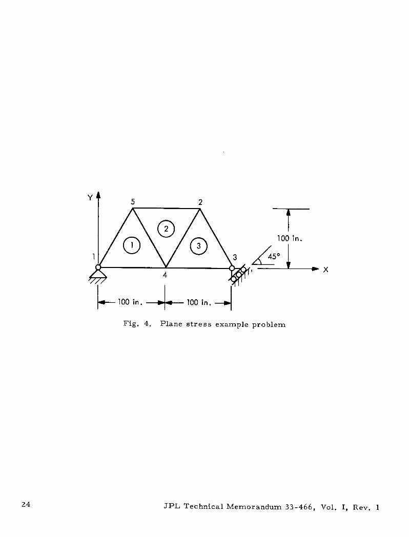
4. Plane stress example problem ...................
5. VISCEL input data for plane stress example problem .....
JPL Technical Memorandum 33-466, Vol. I, Rev. 1
1
2
........ . . . . . . . . . . . . . . . . . . 2
. . . . 2
. . . . 6
. . . . · 9
... . 10
.. . 10
1Z
.. . 15
.. . 15
. . 16
16
17
19
20
21
22
23
24
25
. . . . . .
v

CONTENTS (contd)
Appendix:
TABLES
Various Reference Tables and Figures ..............
A-1. Deflection degrees of freedom at a point for differentcases of structures ...........................
A-2. Types of structures that VISCEL can handle
A-3. Element properties .
A-4. Necessary and optional information for elementdefinition.
A-5. Types of elements available for different cases ofstructures .
A-6 Convention for ordering the vertices of elements .
A-7. The functions of the FORTRAN units as used in VISCEL . . .
A-8. Summary of the problem control card (input item 2) ofinput data ..................................
A-9. Description of element data for different element types . . .
A-10. Table for determining the direction of local y axis and thesign of angle 0 ..............................
A- 1l. List of output items .
A-12. Meanings of the components of stresses at mesh pointsof two- and three-dimensional continua ..............
A-13. List of error messages
FIGURES
A-1.
A-2.
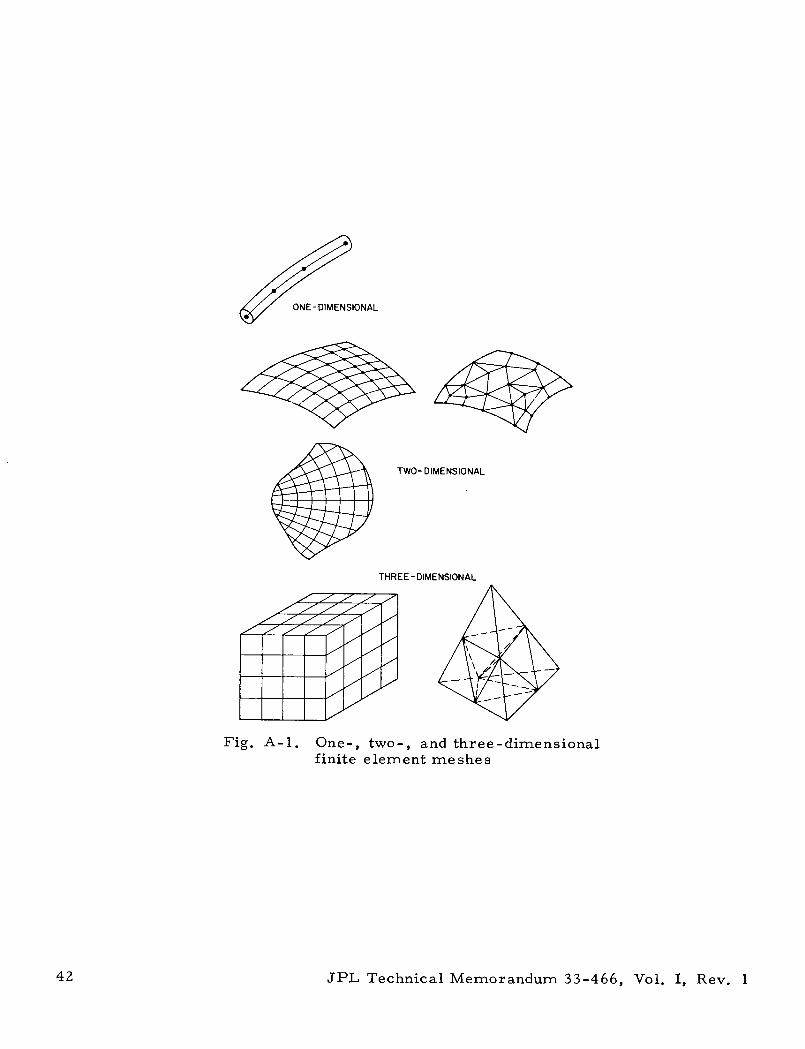
One-, two-, and three-dimensional finite element meshes..
Description of the material ......................
vi JPL Technical Memorandum 33-466, Vol. I, Rev. 1
27
28
29
30
31
32
33
34
35
37
38
39
40
41
42
43

ABSTRACT
This revised user's manual describes the details of a general-purpose
computer program VISCEL (VISCoELastic analysis) which has been devel-
oped for the analysis of equilibrium problems of linear thermoviscoelastic
structures. The program, an extension of the linear equilibrium problem
solver ELAS, is an updated and extended version of its earlier form (written
in FORTRAN II for the IBM 7094 computer). A synchronized material prop-
erty concept utilizing incremental time steps and the finite element matrix
displacement approach has been adopted for the current analysis. Resulting
recursive equations incorporating memory of material properties are solved
at the end of each time step of the general step-by-step procedure in the
time domain. A special option enables employment of constant time steps in
the logarithmic scale, thereby reducing computational efforts resulting from
accumulative material memory effects. A wide variety of structures with
elastic or viscoelastic material properties can be analyzed by VISCEL.
The program is written in FORTRAN V language for the UNIVAC 1108
computer operating under the EXEC 8 system. Dynamic storage allocation
is automatically effected by the program, and the user may request up to
195K core memory in a 260K UNIVAC 1108/EXEC 8 machine. The physical
program VISCEL, consisting of about 7200 instructions, has four distinct
links (segments), and the compiled program occupies a maximum of about
11700 words decimal of core storage. VISCEL is stored on magnetic tape,
and is available from the Computer Software Management and Information
Center (COSMIC).
JPL Technical Memorandum 33-466, Vol. I, Rev. 1 vii

VISCEL - A GENERAL-PURPOSE COMPUTER PROGRAM FOR
ANALYSIS OF LINEAR VISCOELASTIC STRUCTURES
USER'S MANUAL
I. INTRODUCTION
The general-purpose digital computer program VISCEL is capable of
solving equilibrium problems associated with one-, two-, or three-
dimensional linear viscoelastic structures (Fig. A-1). Since the program is
an extension of the linear equilibrium problem solver ELAS (Ref. 1), its sol-
ution at the beginning of the initial time step yields elastic solution of struc-
tures. Basic inputs of VISCEL, thus, are the same as in ELAS; additional
inputs are, however, necessary for VISCEL, which represent changes in
material properties and loading in the time domain. Other important features
of the program include dynamic memory allocation, optional node relabelling
scheme, boundary condition imposition during assembly of the stiffness
matrix and its storage within a variable bandwidth. The program is further
divided into four distinct links, namely, input, generation, deflection, and
stress links.
This user's manual describes the numerical problem formulation, input
preparation, output description, and other relevant details of the program.
The physical program is available from COSMIC. 1
Volume II of this report is the program manual, which contains the
lists of variables, subroutines, and flow charts as well as other pertinent
program information (Ref. 2).
1 Computer Software Management and Information Center, Computer Center,University of Georgia, Athens, Georgia 30601, telephone: (404) 452-3265.
JPL Technical Memorandum 33-466, Vol. I, Rev. 1 1

II. BASIC CAPABILITIES OF THE VISCEL PROGRAM
The basic capabilities and the initial inputs of VISCEL are the same as
the linear equilibrium problem solver ELAS (Ref. 1). In order to achieve a
self-contained report, this report includes several tables and figures from
Ref. 1; they are provided in the Appendix in appropriate order. Thus,
Tables A-1 and A-2 describe, respectively, the various structures that can
be solved by VISCEL and their compatible combinations. Also, information
regarding various available finite elements is given in Tables A-3, A-4, and
A-5. Further, the usual conventions for ordering of element nodes are
explained in Table A-6. VISCEL can handle any material, namely, isotropic,
orthotropic, or anisotropic; their input requirements are described in
Fig. A-2.
III. NUMERICAL FORMULATION OF THE LINEAR THERMOVISCO-ELASTIC PROBLEM
Reference 3 gives complete derivation of the numerical formulations of
the linear thermoviscoelastic problem, whereas Ref. 4 presents details of
the finite element technique. However, such formulations are summarized
below in a simplified manner for completeness of this report.
A. Basic Approach
The fundamental equilibrium problem in structural analysis can be
formulated as differential equations with appropriate boundary conditions;
alternatively, an equivalent extremum formulation may be developed based
on the principle of minimum potential energy and its complement (Ref. 5).
In this work, structural discretization is achieved by the finite element dis-
placement matrix technique, a variant of the well-known Ritz method for the
minimization of the total potential energy functional 4 associated with admis-
sible displacement trial functions. The admissible functions are restricted
to be sufficiently smooth, usually being algebraic or trigonometric polyno-
mials, and, furthermore, they are required to satisfy essential boundary
conditions arising from the requirement of geometric compatibility. This is
achieved by expressing the trial solution in terms of a set of linearly inde-
pendent known functions and undetermined parameters and then minimizing
the functional with respect to such parameters.
JPL Technical Memorandum 33-466, Vol. I, Rev. 12

In the finite element method, a structure is discretized by any suitable
random mesh, and a family of piecewise continuous displacement fields is
prescribed for each element, which are finally expressed in terms of their
nodal function values. Such nodal displacements are the undetermined
parameters to be determined from the extremum principle, the fundamental
assumption in the procedure being that the total potential energy of the entire
structure is equal to the sum of potential energies of the individual elements
(Ref. 4). Such an assumption is valid provided the displacement functions
and their derivatives of order one less than the highest one appearing in the
functional are continuous at interelement boundaries; this ensures that values
of highest derivatives occurring in the total potential energy functional +
remains finite (Ref. 4). Obviously, the greater the number of chosen unde-
termined parameters, i. e., finer the finite element mesh, the lower the
value of the total potential energy would be, yielding even better approxima-
tions. Whereas ~ approaches its minimum value from above, the corres-
ponding strain energy value is always underestimated, and hence the present
approach computes lower bounds of associated displacements. The finite
element procedure thus gives a stationary value of 4 for the variations of the
unknown nodal displacements. Because of its resemblance to the piecewise
Ritz procedure, any particular nodal parameter is only influenced by its
adjacent elements, and hence the final stiffness matrix is highly banded in
nature for most practical problems. It can further be shown that the minim-
ization process of total potential energy of the entire structure with respect
to each unknown nodal displacement is equivalent to the appropriate summa-
tion of such process for all individual elements with respect to their nodal
parameters. For quadratic functionals, the piecewise Ritz procedure for
each element yields symmetric linear equations in the element displacement
vector. The minimization process for the entire structure then leads to the
set of linear, simultaneous equations:
a-= Kq+ P = k eqe+ pe E ( 1)aq
JPL Technical Memorandum 33-466, Vol. I, Rev. 1 3

where
ke = element stiffness matrix
eq = element nodal displacement vector
pe = equivalent nodal load vector
with appropriate summation over all elements based on nodal connectivity.
Such equations are further positive definite for stable structures and may be
solved by standard processes to yield the undetermined nodal displacements.
Computation of stresses, etc., is performed next by the usual procedure.
The program starts with the computation of element stiffness matrices
already derived above.
In viscoelasticity, the creep strain rate or the relaxation stress
response is dependent not only on the current stress and strain state, but
also on the entire history of its development in the time domain. Associated
numerical computation procedures usually adopt a step-by-step incremental
process, which normally requires knowledge of stress and strain at all pre-
ceding intervals. This enables computation of stresses/strains at a given
time implied by some relevant law of the characteristic functions. Usually
such material properties are strongly dependent on time and temperature.
The viscoelastic equations are developed as finite difference equations in
time and finite element matrix equations in space (Ref. 3). This computer
program is based on linear thermoviscoelastic formulations utilizing a
"synchronized" material property concept for thermorheologically simple
materials. The fundamental assumptions may be summarized as follows:
(1) Material properties. The material properties may be
temperature-dependent and are assumed to behave in a thermo-
rheologically simple way; thus, for temperature changes, the
characteristic functions, both creep and relaxation, show pure
shift when they are plotted against the logarithm of time.
Such materials are better suited for a complete characterization
over a large range of time and temperature scale since their
theological behavior can be described for the entire temperature
range as a single function of reduced time and temperature.
JPL Technical Memorandum 33-466, Vol. I, Rev. 14

Thus, when any characteristic function, such as the relaxation
modulus, is plotted against reduced time, all curves will fall on
the single curve for initial temperature T o . Hence it is then
necessary to determine relaxation/creep functions for one tem-
perature only.
The shift functions may sometimes be dependent on stresses,
requiring determination of the shift function at the end of each
time step. However, such considerations are excluded in the
present version of the program. The material can be isotropic,
orthotropic, or general (Fig. A-2), provided they are properly
defined by experimental results. For this analysis, it is
required to have a knowledge of the modulus functions (relaxation-
type functions). Furthermore, the material is assumed to be at
least slightly compressible.
The concept of synchronized material properties is that all
material properties are functions of only one parameter 6. The
same concept applies to external loadings, both mechanical
and/or thermal. The parameter J may be time, reduced time,
or any other suitable variable. Material and load data are con-
sidered in functional form (Fig. 1), which are to be presented at
each time step, in the shape of predetermined tabulated values
obtained either experimentally or derived from analytical con-
siderations; any interaction between them is assumed to be
included in such values.
(2) Linear viscoelastic behavior. Strains are linear functions of
stresses, but are strongly dependent on loading history, implying
that if all loads are doubled, all deformations will be doubled too.
Thus, creep/relaxation laws are linear in stress/strain and as
such the principle of superposition is valid for such cases.
Further geometric nonlinearies, e. g., large strain or large
deformations, are not considered for the current analysis.
(3) Deflection boundary conditions. Deflection boundary conditions
are assumed to remain unaltered throughout the entire time
domain of computation, being fixed initially at the beginning of
JPL Technical Memorandum 33-466, Vol. I, Rev. 1 5

the initial time step. The solution at the beginning of such initial
time step corresponds to the usual linear elastic analysis of the
structure.
B. Analysis Review
Numerical formulation of the step-by-step linear thermoviscoelastic
analysis procedure for quasi-static problems may now be summarized. A
basic assumption in the analysis is that the materials are thermorheologi-
cally simple in nature. Such an assumption is necessary so that the charac-
teristic functions may be singly defined for the entire temperature range in
the time domain. The usual field equations for viscoelastic materials may
then be extended for the thermoviscoelastic case. This is achieved by intro-
ducing the concept of a "reduced time" when all characteristic functions ful-
fill the same time-temperature shift and can be represented as a function of
reduced time:
ft dT
g(xh't) J a[T(xh,T)] (2)
in which a(T) is the time shift function usually determined experimentally as
a function of temperature T only. Such shift function dependence on time t
and position xh
within the material region is implicit through T, and may be
sometimes described by the well-known Williams-Landel-Ferry (WLF)
equation. Relationship (2) signifies that all the characteristic functions,
such as relaxation moduli of a thermoviscoelastic material at any arbitrary
temperature T corresponding to time t, may now be expressed by their
behavior at reference temperature T o on the new reduced time scale i.
Each relaxation modulus, signifying relaxation stress variation for unit
strain applied initially, may then be expressed as
T T 0Eijk2 (t) = Eijk (i = j = k = = 1, 2, 3) (3)
Eijke(t) being the general anisotropic relaxation moduli having 21 independent
components. The constitutive equations for the usual viscoelastic case may
JPL Technical Memorandum 33-466, Vol. I, Rev. 16

be derived by approximating strain variations by the sum of a series of
step functions, which corresponds to a series of relaxation displacement
inputs. Constitutive equations are obtained, from superposition principles,
in the form of hereditary integrals. For the present thermoviscoelastic
case, the constitutive equations may simply be derived from such relations
for the corresponding viscoelastic case by utilizing Eq. (3):
ij (X h t) f Eijk (Xh t) - w(xh, T)]
Xa [ek (xhT) - ak (xh T)O(xh T)] d T (4)
o.. E e~. e + Ek(dT (5)ij iijk( k(O) ijke( aT k - ) (5)
in which ek2 (O) is the initially induced step strain at t = 0, the correspond-
ing first term being the effect of such initial strain at time (xh, t). The
kernel of the hereditary integral Eijk2[ (xh, t) - (Xh, T)] may be considered
as the memory function transforming the influence of pulse strain at time T
to the time instant t. In addition to Eq. (4), two more equations are
required to completely define the field equations:
(1) Equilibrium equations
-. . . + f . = 0 (6)1J, j 1
(2) Strain-displacement equations
1e -(u. + u. ) (7)eij =2 (i, j j, i
where fi is the body force component per unit volume. The field equations
may next be expressed as incremental field equations when the time domain
JPL Technical Memorandum 33-466, Vol. I, Rev. 1 7

is subdivided into arbitrary intervals At(m). Equations (6) and (7) and the
stresses of Eq. (5) then take the following form:
a + af. = 0ij(m), j l(m) = 0
ij(m) 2 i(m),j j(m), i
(8)
tij(n) )
0-ij (n) = Eijk2(9 (n)) ek2(0) + Eijk£( (n) - ') aT (ek - akee) dT
Finally, Eq. (9) may be approximated and expressed in the matrix
form as follows:
m=n
n} = [E(ni)]{eo + E [E(0n - n-l)]{ Aemm=l
- A(a6)m}
The continuum is next divided into small finite elements, and piece-
wise continuous displacement fields are prescribed for each of such ele-
ments in terms of their time-dependent nodal function values. Minimization
of the total potential energy with respect to such parameters then yields the
incremental equilibrium load-deflection equations of the entire structure.
Such step-by-step incremental equations may finally be written in the global
coordinate system:
[Kn, n-l]{AUn = (P} -
n
+Em=l
m=n - 1
m=l[Kn, m-1] {AUm} - [Kn] {U}
4Tn m-} +FnIn, m-lJ + nF
JPL Technical Memorandum 33-466, Vol. I, Rev. 1
(9)
(10)
(11)
8

with
i[K j] = stiffness matrix derived from material matrix computed
for the reduced time difference =Aij
= %j - Ci
Pn}= external load vector at step n
{Tn, m1 }= forces due to temperature changes
{F} = body forces vector
and in which the summation, as usual, signifies the memory of the material.
The element stresses may then be obtained from Eq. (10), when element
strains are derived from the usual relationship:
e eue = XUe
-eU = au
e = bu
U e , ie being element nodal displacements in the global and local coordinate
systems, respectively, Xthe direction cosine matrix, and U and e are
displacements and strains within the element.
C. Special Incremental Procedure
It is apparent from the nature of Eq. (11) that computation time may
be excessive after a few time steps. This is because at each time step,
recomputation of solution results is required for all preceding time steps,
which are then added to obtain the final solution. However, in order to
minimize such computation efforts, the program provides an option by which
time steps may be so chosen that previous time intervals become a subset
JPL Technical Memorandum 33-466, Vol. I, Rev. 1 9

of the following time intervals. Thus, the parameter i may be expressed as
the summation of incremental Al's as follows (Ref. 2):
M N(i) i- )jj i N1i ) j N( i ) A i i ( 1 2 )
i=l j=l
where M defines the total number of time step groups, and N(i) is the number
of steps in the ith group. The values of M and N can be suitably chosen by
the user, and this scheme may be employed to solve the recursive Eqs. (10)
and (11), provided material property and external loads are available for
each jl. Figure 2 shows details of such a computation scheme for values of
M = 3, N(1) = 2, N(2) = 3, and N(3) = 2. In such cases the time intervals
tend to remain constant in the logarithmic scale; thus, it is then possible to
cover a long time domain with relatively small computational effort.
IV. INPUT PREPARATION FOR VISCEL
The program VISCEL is assumed to be stored on a tape (say,
number 12345), which contains the symbolic and relocatable program
elements. Data deck corresponding to any problem must be preceded by
a set of control cards which are first described below. The actual data deck
preparation is explained next.
A. VISCEL Control Cards for UNIVAC 1108/EXEC 8 Computer
Depending on the size of the problem to be solved, the user may
request for an appropriate core storage. Such values are assigned to an
integer LDATA, to be calculated approximately from Ref. 2, Fig. 1, in
which for most problems the major storage space would be required for
elements of the upper symmetric half of the stiffness matrix. The program
is compiled for LDATA = 20000 words decimal storage, and if more storage
is requested, this is achieved by recompilation of two small programs
COMBK and MAIN, the block data and the main driver programs,
respectively.
Furthermore, as explained in Ref. 2 (pp. 3-4), various Fastrand
(drum) file storage units are utilized as additional stores during execution
JPL Technical Memorandum 33-466, Vol. I, Rev. 110

of the program; their functions are summarized in Table A-7. Unless
specified, the UNIVAC 1108 system automatically allocates 128 tracks to
each of the units, which, however, may be inadequate for solution of large
order problems. It is then necessary to increase the number of data tracks
for such units by inserting relevant control cards in the run stream.
Control cards corresponding to the two sets of values of LDATA are
as follows:
(1)
not requir
Control cards with LDATA < 20000
The following run stream may be used for problems which do
:e more than 20000 words storage for the COMMON:
@RUN,/TPC RUNID, ACCOUNT, PROJECT, TIME, PAGES
@MSG, READ TAPE 12345
@ASG, T TAPE, T, 12345R
@ FREE TPF$
@ASG, T TPF$, F///500
@ COPY, G TAPE, TPF$
@ FREE TAPE
I @ASG, T UNIT NUMBER, F2///1000
@XQT ABSEL
VISCEL INPUT CARDS
@FIN
(2) Card input with LDATA > 20000 (say, LDATA = 80000)
When COMMON requirements are greater than 20000 (say,
80000), the following typical run stream may be adopted:
@RUN, /TPC RUNID, ACCOUNT, PROJECT, TIME, PAGES
@MSG, READ TAPE 12345
@ASG, T TAPE, T, 12345R
@ FREE TPF$
@ASG, T TPF$, F///500
JPL Technical Memorandum 33-466, Vol. I, Rev. 1 11

@COPY, G TAPE, TPF$
@FREE TAPE
L@ASG, T UNIT NUMBER, F2///lOOOj
@FOR, S COMBK, COMBK, COMBK
-2, 2
PARAMETER LDATA = 80000
@FOR, S MAIN, MAIN, MAIN
-2, 2
PARAMETER LDATA = 80000
@PACK
@PREP
@MAP, EN MAPEL, ABSEL
@XQT ABSEL
VISCEL INPUT CARDS
@FIN
Requests for additional storage tracks for the Fastrand units may be made
by inserting control cards, shown above within the dotted boundaries.
B. Input of Problem Data
The physical arrangement of the data deck which follows the control
cards (explained in previous section) is depicted in Fig. 3. This deck
corresponds to values M = 2, N(1) = 2, N(2) = 3 in the time domain
defined by Eq. (12). VISCEL input data may be as described below, with
reference to Table 1 describing input items; the integers of the problem
control card (Table 1, input item 2) is explained in Table A-8.
Data Group 1: Basic input for the elastic problem which also
corresponds to the initial time solution of the
viscoelastic problem
JPL Technical Memorandum 33-466, Vol. I, Rev. 112

Data Group 2: Data for multiple solutions of the elastic problem
or
Data for viscoelastic incremental solution in the
time domain
The nature of the data in group 2, if any, is determined by the con-
tents (ISUCA value) of the END card in the master (initial time) deck (input
item 19, Table 1) and the subsequent additional input data decks for visco-
elastic problems. Field specification for the END card is as follows:
70X, 17, 3HEND (13)
in which the I7 field corresponds to the integer ISUCA, which is to be set
as follows:
(1) ISUCA = 0 For linear elastic problems
(2) ISUCA < 0 For multiple runs
(3) ISUCA > 0 For linear viscoelastic problems
(4) ISUCA = 1 For master and following deck
(5) ISUCA > 1 For following additional decks in increasing
sequence
Thus, in the viscoelastic case, the first card following the data of
the previous time step is the problem control card, equivalent to input
item 2 of the initial time step, containing information on modifiable input
items. The modified information is provided next, followed by the END
card with the ISUCA value which determines the nature of the data, if any,
in the succeeding step. A numerical example of a two-dimensional plane
stress problem (Fig. 4) with irregular mesh labeling is chosen to elaborate
on the preparation of the data; the complete input data are presented in
Fig. 5 with M = 2, N(1) = 4, and N(2) = 2 values selected for the incre-
mental time scheme of Eq. (12). Node relabeling may be requested by
using appropriate option in input item 17 of Table 1.
Relevant details on permanent and modifiable input items are provided
in Table 2. Element data corresponding to input item 16 of Table 1 is
described in Table A-9. Also, input items 13, 15, and 18 in the same table
may be specifically described as follows:
JPL Technical Memorandum 33-466, Vol. I, Rev. 1 13

(1) Input item 13 (angle types - fixing local y and z axes)
In connection with element type 4 (Table A-3), the input corre-
sponding to column 16 of Table A-4 consists of a list of + angles
in degree units. The 4 values are assigned quantities with abso-
lute values less than 90 deg and. are defined as the angle between
the local y and. global Y axes. Let the direction cosine vectors
be denoted by (fxX' fxY' lxZ)' (1yX' fyY' Iyz ) and ( zX' £zY' izZ)
in which the local x axis is assumed. to coincide with the nodal
line 1-2 (Table A-3). Then the signs of fxX' yX' and Ify are
used. to determine the sign of q; such procedure is summarized
in Table A-10.
(2) Input item 15 (deflection boundary conditions)
The deflection boundary condition relations may be written as
(Ref. 1):
u, j = + aui + a2ui, j + (14)
when coefficients a, al, a2
. , and the input pairs (i,j),
(i',j'), (i",j"), .. ., are the relevant inputs as follows:
i,j i,j a0
i, j i',j' a1
i,j i", j" a 2
in which the first two pairs along each row are the two degrees
of freedom, under consideration and the related one, the third
scaler relating such two deflection components.
JPL Technical Memorandum 33-466, Vol. I, Rev. 114

(3) Input item 18 (concentrated load input)
The inputs for the prescribed force boundary conditions for
concentrated loads are as follows:
i,j P
i',j' P'
where P., I twhere Pij Pi.,j I , ... , are the prescribed. concentrated nodal
loads at nodes i, it , ... , corresponding to degrees of freedom
j,j't ,..., respectively. Apart from concentrated. loads, the ele-
ments may be subjected. to any pressure as well as temperature
loading as indicated, in Table A-4.
V. DESCRIPTION OF VISCEL OUTPUT
Table A-11 provides a list of output items of the initial time step
solution, whereas Table 3 summarizes such items for the entire visco-
elastic problem with an input index value INP set to 1 for the elastic solution.
The definition of stress components at mesh points is given in Table A-1Z.
VI. ERROR MESSAGES AND DIAGNOSTICS
The error messages shown in Table A-13 are usually related to the
initial time step solution. Error message 10 in particular needs a detailed
explanation, which appears either for geometrically unstable structures, or
when the structure is not adequately supported. The last number appearing
in the error message, if negative, indicates the mesh number to be checked
carefully for existence of any unknown deformation. However, if the num-
ber is positive, then it is first necessary to find from output item 10 of
Table A-11 the pair of numbers with the second number identical to this
error message number. The first number of the pair is called IBB,
denoting the equation number in the reduced set of the stiffness matrix.
Then column IBB of output item 10 of Table A-11 is searched for the row
having the same IBB number found previously, such that the column IBO
contains the number -1. The mesh number in that row happens to be the
trouble spot, whereas the defective direction is the one appearing in the
JPL Technical Memorandum 33-466, Vol. I, Rev. 1 15

table heading of the output item. In such case, the element descriptions,
material matrices, and geometric continuity around the mesh point are to
be checked to correct the situation.
VII. CONCLUDING REMARKS
This user's manual describes in detail the information necessary to
utilize the computer program VISCEL for the solution of thermoviscoelastic
problems associated with practical structures. Extensive applications of
the problem are envisaged in the analysis of a wide variety of practical
structures including solid propellant rocket motors, spacecraft components
such as solar panels, etc. In order to make this document complete, some
information, including most tables and figures in the Appendix, have been
reproduced from Ref. 1.
REFERENCES
1. Utku, S., and Akyuz, F.A., ELAS -A General-Purpose ComputerProgram for the Equilibrium Problems of Linear Structures:Vol. I. User's Manual, Technical Report 32-1240. Jet PropulsionLaboratory, Pasadena, Calif., Feb. 1, 1968.
2. Gupta, K.K., and Akyuz, F.A., VISCEL--A General-PurposeComputer Program for Analysis of Linear Viscoelastic Structures:Vol. II. Program Manual, Technical Memorandum 33-466. JetPropulsion Laboratory, Pasadena, Calif., July 15, 1972.
3. Heer, E., and Chen, J. C., Finite Element Formulation for LinearThermoviscoelastic Materials, Technical Report 32-1381. JetPropulsion Laboratory, Pasadena, Calif., June 1, 1969.
4. Zienkiewicz, O. C., The Finite Element Method in EngineeringScience. McGraw-Hill Book Co., Inc., New York, 1971.
5. Crandall, S.H., Engineering Analysis. McGraw-Hill Book Co., Inc.,New York, 1956.
JPL Technical Memorandum 33-466, Vol. I, Rev. 116

Table 1. Input items (summary of options, contents, and formats)
Input Conditions Formatitem determining List of input statements that read the associated input item card(s)' (outside parentheses indicate theNo. options possibility of multiple cards)
1 (Bi, i = 1, 14) The card may contain any alphanumeric message 14A6
2 IN, IT, IDEG, ITYPE, IGEM, ISTR, IH, 18, IBN, IP, IPRS, IMAT, NTIC, 214, 611, 314, 1012, 911, 3F5.4, E10.5ISDT, ISDY, ISDZ, IARE, IMMX, IMMY, IMMZ, IMFI, INX, INP, ISHUF, (see Table A-8 for details)ICOR, B1UN, IMES, IPIR, ITAP, ITAS, G1, G2, G3, ACEL
3 b ITYPE = 0 (i, Ei, Gi, a
i, i = 1, IMAT) (3(12, 3E8.5))
ITYPE = 1 (i, D1i, D 2i, D14i, D22,, D24i D44, D' D06 D66i'"al, (12, 9E8.5/12, 2E8.5)
a2, i= 1, IMAT)
ITYPE = 2 (i, D0,, D1 D3i, D24i , D D22i, D23i D24i i, D2i (12, 9E8.5/12, 9E8.5/12, 6E8.5)
D26i, D 3 3 i, D34i, D 3 5i, D36i' D44i, D 45i D4 6 i, i, D 5 5 ,i D5,6i
D66 i, 5ai, a ,, i = 1, IMAT)
4 1 < IPRS < 99 (i, Pi, i = 1, IPRS) (8(12, E8.5))
IPRS = 0 No input card
5 1 < NTIC < 99 (i, h i , i = 1, NTIC) (8(12, E8.5))
NTIC = 0 No input card
6 1 < ISDT < 99 (i At, i = 1, ISDT) (8(12, E8.5))
ISDT = 0 No input card
7 1 < ISDY < 99 (i, (ct/ay)i, i = 1, ISDY) (8(12, E8.5))
ISDY = 0 No input card
8 1 < ISDZ < 99 (i, (at/az)i, i = 1, ISDZ) (8(12, E8.5))
ISDZ = 0 No input card
9 1 < IARE < 99 (i, Ai, i = 1, IARE) (8(12, E8.5))
IARE = 0 No input card
10 1 < IMMX < 99 (i, Ci, i = 1, IMMX) (8(12, E8.5))
IMMX = 0 No input card
11 1 < IMMY < 99 (i, IC, i = 1, IMMY) (8(12, E8.5))
IMMY = 0 No input card
12 1 < IMMZ < 99 (i, l i = 1, IMMZ) (8(12, E8.5))
IMMZ = 0 No input card
13 1 < IMFI < 99 (i, I i = 1, IMFI) | (8(12, E8.5))
IMFI = 0 No input card
14 ICOR = 0 (j, , Yj,Zj, j = 1, IN (14, 3E12.4, 40X) or (40X, 14, 3E12.4) or2 < IN < 9999 (2(14, 3E12.4))
ICOR = 1 Input card(s) should be as required by the user's version of subroutine CORG (see Ref. 1)
JPL Technical Memorandum 33-466, Vol. I, Rev. 1 17

Table 1 (contd)
Input Conditions Format
item determining List of input statements that read the associated input item card(s)" (outside parentheses indicate the
No. options possibility of multiple cards)
15 IBUN = 0 (ikiki Iakk 1, BN) (5(14,11, 14, 11, F6.0))1 < IBN < 9999
IBUN = 1 Input card(s) should be as required by the user's version of subroutine BUNG (see Ref. 1)
16 IMES = 0 (MM,,, J W,,,, J2 W,,, J3W,,, J4W.,,, J5W, ..... m = 1, IT) (2014) (see Table A-9 for variables of
1 < IT < 9999 | the list)
IMES = 1 Input card(s) should be as required by the user's version of subroutine MESG (see Ref. 1)
17 ISHUF = 0or 1 No input card
ISHUF = 2 (Ni, i = 1, IN) (2014)
ISHUF = 3 (N i , IMAX i , i = 1, IN) (2014)
18 1 < IP < 9999 (il, j, P, I = 1, IP) (5(14, 11, E11.4))
iP = 0 No input card
19 No list (the card is punched END in the last three columns) 70X, 17, 3HEND (ISUCA value)
20 No input for standard VISCEL; otherwise input of certain user's subroutines (see Ref. 1)
VISCEL PROBLEM CONTROL CARD, PROVIDES MODIFIABLE INFORMATION
MODIFIED INFORMATIONS
19 END card 70X, 17, 3HEND (ISUCA value)
PROCESS TO BE REPEATED
FOR SUBSEQUENT TIME STEPS
aNomenclature
p pressure 1, moment of inertia about local z axis
h thickness ¢ angle determining the orientation of principal axes of cross section
At temperature increase in overall coordinate system
a t/dy temperature gradient in local y-axis direction X, Y, Z overall coordinates of mesh points
d t/dz temperature gradient in local z-axis direction x, y, z local coordinatesA cross-sectional area ,, , index pairs and the constant of the kth dbc input unit (see SectionA cross-sectional area II-D)
Ill-D)
C torsional constant il,j1 ,P, index pair and constant of the Ith concentrated load input unit (see
I, moment of inertia about local y axis Section IV-B)
bThe symbols shown in Input Item 3 are defined in Figs. A-2c, 2d, and 2e.
JPL Technical Memorandum 33-466, Vol. I, Rev. 118

Table 2. Permanent and. modifiable input items
Description of input item Qualifications
Existencein themasterdeck
Existencein the
successivedecks
1 Title card For master deck only *
2 Control card For master and successive decks * *
Modifiable information
3 Material types For master and successive decks o
4 Pressure types For master and successive decks o o
5 Thickness types For master and successive decks o o
6 Temperature increase types For master and successive decks o o
7 Temperature gradient types For master and successive decks o o-local y-axis direction
8 Temperature gradient types For master and successive decks o o-local z-axis direction
9 Cross-sectional area types For master and successive decks o o
10 Torsional constant types For master and successive decks o o
11 y-moment-of-inertia types For master and successive decks o o
12 z-moment-of-inertia types For master and successive decks o o
13 Angle types-fixing local y and For master and successive decks o oz axes
Permanent information
14 Mesh point coordinates For master deck only o
15 Deflection boundary conditions For master deck only o
16 Element descriptions For master deck only o
17 Relabelling information For master deck only o
Modifiable information
18 Concentrated loads For master and successive decks o o
19 End card For master and successive decks * *
* = the card(s) must exist.
o = the card(s) exist optionally depending on the control constant in the control card and relate to themodifiable information.
- = the card(s) must not exist.
JPL Technical Memorandum 33-466, Vol. I, Rev. 1
Input itemnumber
19

Table 3. Summary of output items
Output Output for linear elastic solution or Output for linearitem initial time solution of linear iscoelastic solution
number viscoelastic problems
Linear elastic problem or linear visco-elastic problem
(1) Title of the problem(2) Table for control constants
Modifiable information (material prop-erties, pressure types, etc.)
Nodal coordinates
Mesh topology; element property types
Relabelling message
Topology of the reduced stiffness matrix
Stiffness matrix requires.... storagelocations
Total common length is (decimal)....storage locations
Count of main diagonal elements of rowlisted stiffness matrix
Force and displacement boundary condi-tions in directions 1 (2, 3,4, 5, 6)
Input link took.... seconds
Generation link took .... seconds
Nodal deflections
Forces acting at the nodes
Deflection link took.... seconds
Stresses at the nodes
Stress link took.... seconds
Number of equal time stepgroup....
Number of time steps in thegroup ....
Modifiable information (mate-rial properties, pressuretypes, etc.)
Input link took.... seconds
Generation link took.... seconds
Accumulative nodal deflections
Forces acting at the nodes
Deflection link took.... seconds
Stresses at the nodes
Stress link took.... seconds
JPL Technical Memorandum 33-466, Vol. I, Rev. 1
1
2
3
4
5
6
7
8
9
10
13
17
19
20
21
22
25
j
20

t4
(a) ELASTIC MODULUS
(b) SHEAR MODULUS
CC(c) COEFFICIENT OF EXPANSION
(d) EXTERNAL PRESSURE
Fig. 1. Schematic representation of thematerial properties and externaldisturbances at it
(e) TEMPERATURE CHANGE
(f) OTHER PROPERTIES (MODIFIABLE),CONCENTRATED LOAD, ETC.
JPL Technical Memorandum 33-466, Vol. I, Rev. 1
E
G
a
p
T
P
.1
21

'GROUP 3 "
'TYPICAL MATERIAL PROPERTY OR EXTERNAL DISTURBANCE CURVE (CM)
E
=41 :2
t_2t(12 1i- =2 i=36Fig. 2. Typical interval setup
Fig. 2. Typical ~ interval setup
JPL Technical Memorandum 33-466, Vol. I, Rev. 122

Fig. 3. Physical arrangement of data deck for the VISCEL program
JPL Technical Memorandum 33-466, Vol. I, Rev. 1 23
Y 5 2
4
100 in. I_ 100 in.
Fig. 4. Plane stress example problem
JPL Technical Memorandum 33-466, Vol. I, Rev. 1
100 in.
X1
24

ooII 11
) LU
Il) I-Cl
o - I I 1 1
L0
ru
II IIl.oa
..~j
0uJ
N
II II
0 0
D
w~LACn
',
-e -
1W1 I 1
I -u
I
4-UJ
i1
ruFN1
w
ZOIIIW ll
I I I
I I I
1 1-1
m
1 1 l
l I
I I
-1
J +
1
I I
I I
I I
I 'I
I I
I I
+1
I
I I
I I
N
o0
wU
.U_
121 I laSilm
i
I {
p L
l I
I *I I
1!.!;I
I IX
T1
I I
I 1l1
I I
I I
I I
I IIII
oo
LU
Na
e,1
rL
I N
r Lo
1J
oo
l
I I
I I
i 1
1 1 I
I I
I I
I I
::dA
I o ¢
rj oCo
LE+
I -_ I 0
o l-
ol
=
N_
0
N
-O
+ _
_U
n _
aE
NIO
3I
c +
+
+ +
+
+
+
+
+
+L
.I LuJ Lu
LuJ
ul
-uI
Lu
LU LU
1I
I T
0
T
NI
1-
I N
m
In
N
aN
O
I
N
e e+E
rr nr S
llII--7
I--Ji
02zs
u:0j
w0 4
cc
2 <
-
40
cw
0
0 D.
Ez
LU LU
I-
I
LU
o w
II �-
.z2one
049xw
zreclM
ad-
JPL
T
ech
nic
al M
em
ora
ndum
33-4
66,
Vol.
I, R
ev.
1
oz
0
-
I4II222222 7I
9IIII1;822I2IiI,
NL_
=
I
ILL
dV
lI
Nn81
dNI
AWW
IIU
Ii;_
a)
-o0i--i
a)U)
a()0--4o;4o- ML)
13L
CIwN -
.L~AI tq
22II2II
C
dl
HII
ZI O|
I I I I I I I I
I |r O | I I I I
I N
II I I N
_01111
1 11
.I1
.-1.
T-
LU
-II-
Z-J
0z0
iaL
LU-
0.Cr
I I I
I I
I I I
I 1 -n i 1
1 u1
I I .I
I I
I I
I I
I I 0 1 I
I 1-1
E| L
T=
o
4 -I
i T
+
1
IiI.19pIII.IaI.9.RIIII
IIPIIIIPIPIP1i
ore~
-jI
'tF-I1-I.Z_-
DIII ,I7FI7r'.
.4-Z
0
11IiIL
9
E 1:
25

II II
U
0.kLU
0
IIl Z I
IL
UV
rI
FE
[
+iL
UI C
lJ N
IL
ti
zLu
N
N
-II
II
LU
C
-=A
VCC
p-i
iU
N
NII
II
U
.
Ca
-
--=
-rFE,
I1 1 1 )
I I
I+tU
.
LI]I
N~-
u.T-l I
--~J~
TIIErV
ulI
EE "VIE
1+===2
1l
_ T
r
I X
Ll
I c
Is
I _ _
| I
L1
v I
2 L
aWn
_ I
_ 2 II
nw
0
w
-V
N
r 0
r_ 0N
C
1
_
n _N
N
N
N
_
n N
N
N
S
+ +
+ _
_ +
+
+ +
Cr
_ N
e
N
N
N
_ N
LU U
U
U
U
U
J Ir,
_ _
0 0o
=o
.
0
.n 0
N
_ 0
N
_ N
|
.a
O
N
N
d O
av
r =
_
_1
_
_ _
_ _
1
_
0 At
M
z 0
2 0Z
L
Z
0 0
w
wL
U'
LUI LU
0 2
cc L
, ...
9 Ca
C
I
-j00c
422
z
JPL
T
ech
nic
al M
em
ora
ndum
33
-46
6,
Vol.
I, R
ev.
1
-rM
II II
C C-
cL4C
n=
=Z
z
EC
CCJIC
2IG89
F0-
430o,- C)
by-4
,
i I
zl Z
I9
OH
I-r
IrX
1 1
=
o8I
24Ii:
I I
M
I X
:IT
-1
I I
I I
I I
I I
I I
I I
I I
I I
I I
1
2II9Ii21IIIIIa2IIIIIi71i4RI9AI
API
R99AI
IAI
IIII9VII
I -I :4
CPI!Z
I9i!IIIIG
I I-IIII-I-a -
II-1313-I-9-9-IA-
IIR-
I-I-Ii7
1-rrL- -10 e-T
'1C
.7aIII WI
IIIIII::1
u
iGI
2
5Io
tK1
Is
IIr+
-+
-I
jIIIIIIIIII
26

APPENDIX
VARIOUS REFERENCE TABLES AND FIGURES
JPL Technical Memorandum 33-466, Vol. I, Rev. 1 27

Table A-1. Deflection degrees of freedom at a pointfor different cases of structures
Column number 1 2 3 4 5 6 7
E
,~-au 0) ° e E E E 0
o \ .o - as w r ,- a
E E E 0
Case a 0 0
description r E0~ 0~ 0 r Co wo z
1 Planar truss 2
2 Space truss :::. : R8?:_ _ 3
3 Planar frame 3
4 Space frame 6
5 Gridwork frame I I I 3
6 Plane stress R : 8:: 2
7 Plane strain ''' R 2
8 Plate bending 3
9 General solid 9 9 : 3
10 General shell;bend. memb............
11 General shell, membrane ; : R 3
12 Solid of revolution 2
13 Shell of revolution, membrane 2
14 Shell of rev.; bend., memb. 3
4X, Y, Z refer to the axes of the overall coordinate system.
JPL Technical Memorandum 33-466, Vol. I, Rev. 128

Table A-2. Types of structures that VISCEL can handle
11 12 13 14
E E
E E
1E E
4 5pace frame __ ......E,
51 Gridwork fDram ion ,R _
Planar truss- -
8 Plate bending -a. aR i _ g _ g av&'+r~s-v Ra ....................12 Spl a e strss
7 Planar framns (e. 04 41 0 0 0
Se Plate ben g :
1~ase 2 S o li o fi re o lutis
1 3 Shell ofDeseroltion membrane
5 1 Gridwork frame ! ... . . ...... .....
1 Plane stress:
14 Spae framev t; bending, membrane
14 Shell of revolution; bending, membrane
1Cases 6 and 7 may not exist simultaneously.
JPL Technical Memorandum 33-466, Vol. I, Rev. 1
1 2 1 3 4 1 5 1 6 1 7 1 8 1 9 110Case numberI
L
29

0 .
o N
0 o
0
0c
_ 0
>
.- o
c
O
oO
0
e-o0
0Eo o
_00 .
00noIF0I
ZI
.'E0
-o
Dre
ex o
9 0.
g,o
o ~.~Et 7e -
0 0
0
o f9
0 *
o~
D_
e e
0-
e'0
-
D0"
.0,
&
-o
oD_
.- .C
0.
0 0
E
0 _
NO >
0 D
0
0 *.
'0
0 0~
~~
~
-u
ew
ep
e jo
w
eis
As elu
!pJooI0
l Li
0 0
i U
U
U
U
<
< <1
< (ulul
t uer~
sesupoo
D~
l ·
· []
[] [
· ·
· ·
· ·
~3 3
c3 q
· ·
4 '
i:e oin
pn
jip 04 podB
sJ 44!M
WeIsA
s >.
.*
' *
..
o 0
0 0
0 0
0 0
0e)D
u!pJ00oo IID
JeAO
JO
uo
UojuIa!J0
') 0
0 I
ID
0 s!.o
Aowl e
inssa
id
944
qIP4m
P [
~ (
( (
uo euD
ld ID
pou JO
eU
l IDPON
..
..I
.,
.-
-- -
--
N
u0!48Jrp
S!Ix
(N (N
(N (N
'2 (
y (N 0N
(N
sN
(N
· ··
· ··
·ID
!JGID
WlS
J! P
U
0o4 U
U!I[
p ·
1P
ON
_
a pesn
eq A
ow
UluewIG S!L4I W
!Lm
JoI C
N
(Z-III
elqo
J) ezn
4.n
J4s
*0
'ON
esD
3
0
l1 'U
°!4d
!1~
sep91
logdw
ap
1 0
'0
91 0
'0 N
'
N
' '0
N
, '0
P
I '
N
(f In)
ueWO
ele JO
j spAo/
Jo J0qtw
nN
o oal 'e
pou je
d w
op
ee
q
JO se
eJB
eo(
( (
0 C
(o
r(
(N
n (
'0 '0
C. (N
(
(N C
N
,)
SW
I '(se9
!'BA
e) sO
epou JO
Jqw
nN
c
N
N
( V
(N
0C
( (N
) (
.(
(N
c c c c~~~~~~~~~oa
....i
r
-0:
E
0 E
0
0 m
E
E
C4
Aj~
eoeS
4u9u~
j3
* 0)
9)
9 0
0 0
0 09
0 0
E
0 2 o
0
X~lewoe84uewel~l E
E
E
E
E
'
a
-- 3ji3O
eqwnu
odA,
3I-I-
IMI1
(2
I oI
raqw
unu
edA
l 4uaw
91
1 -
-( N
(N
'0
91 '0
N,
0 0
0 oI
-( N
(N
n
01 '0
N
0
JP
L T
ech
nic
al M
em
ora
nd
um
33-4
66,
Vol.
I, R
ev
. 1
0D
o-o.oc
.o
[] oXq o2
[:1
0]S-4I
.Q cE
-o 11Hu
30
I
i

Table A-4. Necessary and optional information for element definition
1 2 3 4 5 6 7 8 9 10 11 12 13 14 15 16 17 1 18 19 20
EA -t
2 . A Ac E 8
0 3 3
C CP~~~~
>. .>.., = ~ ~ A A . C. - - .-xS x S, S S A * x Cx C 3
...C I> :.- -f t t - -
-E c E --E -3~~~~~ ~~~ ~~~~~~~ ) C0. . 0 .
£ - .W. >. >. cc C E e 0C - - - - - Z
C -0I, -0 I
A. - z -z z z u, . 0 ~ . .-L
2 ~ ~~~~ ~~ 2:::*::::.;:::::::::2
>.- .2U C ~ A A A A A A A -- a a1 aP a a a a 0 .3 : * * *
* ;:2:: C:C:C:C::C;C:* :: 02::: a 0. 0E Ea E w ! E E* 0 0 0 0 0 ~~ ~~ ~~~~0 0 0 2 C * *
2
.......... ........ .........i .......... in f
.-. .. . .. . .. . .
...... ........ ......... ................ .. . .. .... ... ..... ....... ... . .... ....... .... ... . . .6 . ................ . . .. ii i ,.... .. .... .. . .... ...7
8
10
1 2
13
14
15
16
17
18 f' //E3 Necessary inform ation Optional information
JPL Technical Memorandum 33-466, Vol. I, Rev. 1 31

Table A-5. Types of elements available fordifferent cases of structures
Column number 1 2 3 4 5 6 7 8
E dm E!escri ' *E E
4 Space sfr e 2 C -4description r f r m
1 Planar truss .
2 Space truss
3 Planar frame
4 Space frame
5 Gridwork frame
6 Plane stress
7 Plane strain i i _
8 Plate bending
9 General solid 1
10 General shell; bending, membrane
11 General shell, membrane
12 Solid of revolution
13 1Shell of revolution, membrane '
14 Shell of revolution; bending, membrane _ !,
JPL Technical Memorandum 33-466, Vol. I, Rev. 132

Table A-6. Convention for ordering thevertices of elements
Element
type First Other verticesnumber vertex
1 Any The remaining
2 Any The remaining
3 Any The remaining
4 Any The remaining
5 Any Counterclockwise sequence about overall Z axis
6 Any Counterclockwise sequence about overall Z axis
7 Any Counterclockwise sequence about overall Z axis
8 Any Counterclockwise sequence about overall Z axis
9 Any Counterclockwise sequence for the first three vertices
about the normal of their plane, heading towards
the fourth vertex
10 Any *
11 Any Clockwise sequence about local normal**
12 Any Counterclockwise sequence about local normal**
13 Any Counterclockwise sequence about local normal**
14 Any Counterclockwise sequence about local normal**
15 Any Counterclockwise sequence about overall Z axis
16 Any Counterclockwise sequence about overall Z axis
17 *** The remaining
18 The remaining
*Counterclockwise sequence for the first four vertices on the same faceabout the normal heading towards the other four vertices. The fifthvertex lies diagonally across the first vertex. The last four vertices alsoestablish a counterclockwise sequence about the normal of their face,heading towards the first four vertices.
**Local normals head always to the same side of the space divided bythe middle surface.
***The one with smaller meridional arc length (the meridional curve shouldhave a direction).
JPL Technical Memorandum 33-466, Vol. I, Rev. 1 33

Table A-7. The functions of the FORTRAN units as used in VISCEL
JPL Technical Memorandum 33-466, Vol. I, Rev. 1
FORT RANunit Function of the unit
number
1 System
2 Chain
3 Scratch for topological information generated in Link 3
4 Storage for deflections
5 Input
6 Output
7 Punch
8 Overlays for FORTRAN IV
9 Storage for material elastic constants
10 Storage for material expansion coefficients
11 Storage for temperature changes
12 Storage for elemental stiffness matrices
13 Storage for overall stiffness matrices
14 Scratch for elemental stiffness matrices
Scratch for incremental deflections for ISTEP = 1
15 Storage for stiffness matrix decomposed by Choleski scheme
34
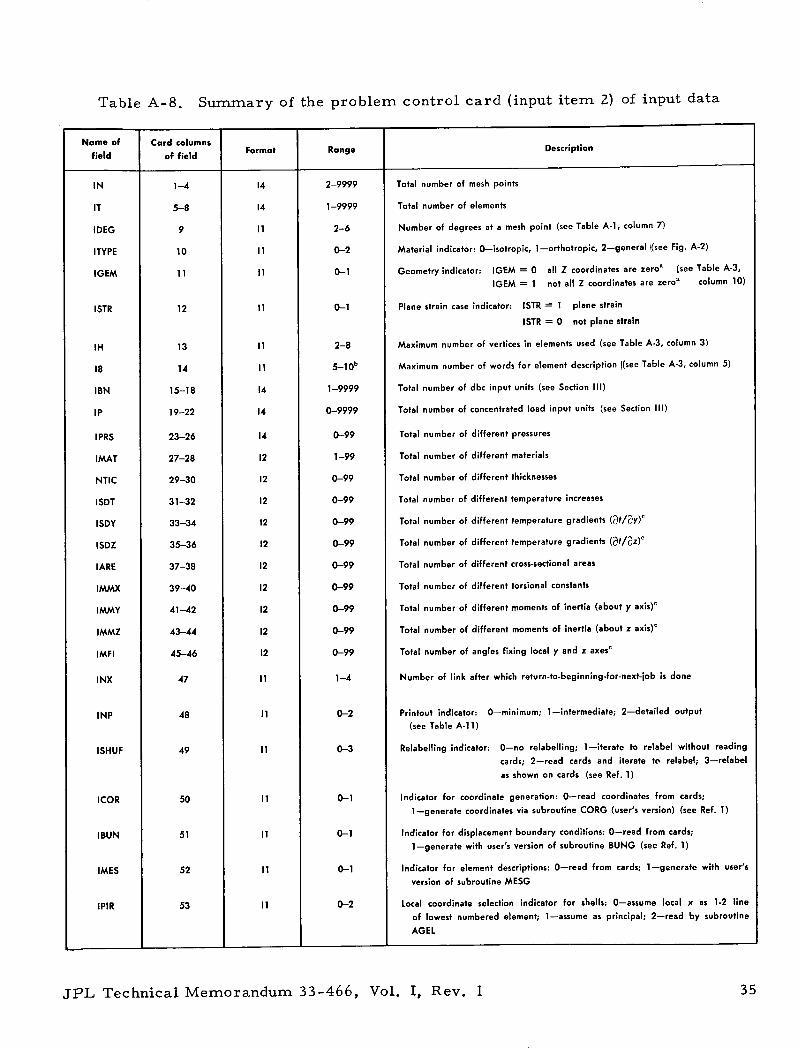
Table A-8. Summary of the problem control card. (input item 2) of input data
Name of Card columnsfield of field Format Range Description
-IIN 1-4 14 2-9999 Total number of mesh points
IT 5-8 14 1-9999 Total number of elements
IDEG 9 11 2-6 Number of degrees at a mesh point (see Table A-1, column 7)
ITYPE 10 11 0-2 Material indicator: 0-isotropic, 1-orthotropic, 2-general (see Fig. A-2)
IGEM 11 0-1 Geometry indicator: IGEM = 0 all Z coordinates are zeroa (see Table A-3,IGEM = 1 not all Z coordinates are zero a column 10)
ISTR 12 11 0-1 Plane strain case indicator: ISTR = 1 plane strain
ISTR = 0 not plane strain
IH 13 11 2-8 Maximum number of vertices in elements used (see Table A-3, column 3)
18 14 11 5-10 b Maximum number of words for element description I(see Table A-3, column 5)
IBN 15-18 14 1-9999 Total number of dbc input units (see Section III)
IP 19-22 14 0-9999 Total number of concentrated load input units (see Section III)
IPRS 23-26 14 0-99 Total number of different pressures
IMAT 27-28 12 1-99 Total number of different materials
NTIC 29-30 12 0-99 Total number of different thicknesses
ISDT 31-32 12 0-99 Total number of different temperature increases
ISDY 33-34 12 0-99 Total number of different temperature gradients (at/ly)'
ISDZ 35-36 12 0-99 Total number of different temperature gradients (at/az)e
IARE 37-38 12 0-99 Total number of different cross-sectional areas
IMMX 39-40 12 0-99 Total number of different torsional constants
IMMY 41-42 12 0-99 Total number of different moments of inertia (about y axis)'
IMMZ 43-44 12 0-99 Total number of different moments of inertia (about z axis)C
IMFI 45-46 12 0-99 Total number of angles fixing local y and z axes'
INX 47 II 1-4 Number of link after which return-to-beginning-for-next-job is done
INP 48 11 0-2 Printout indicator: 0-minimum; 1-intermediate; 2-detailed output(see Table A-11)
ISHUF 49 11 0-3 Relabelling indicator: 0-no relabelling; 1-iterate to relabel without readingcards; 2-read cards and iterate to relabel; 3-relabelas shown on cards (see Ref. 1)
ICOR 50 11 0-1 Indicator for coordinate generation: 0-read coordinates from cards;1-generate coordinates via subroutine CORG (user's version) (see Ref. 1)
IBUN 51 11 0-1 Indicator for displacement boundary conditions: 0-read from cards;1-generate with user's version of subroutine BUNG (see Ref. 1)
IMES 52 1 II 0-1 Indicator for element descriptions: 0-read from cards; 1-generate with user'sversion of subroutine MESG
IPIR 53 11 0-2 Local coordinate selection indicator for shells: 0-assume local x as 1-2 lineof lowest numbered element; 1-assume as principal; 2-read by subroutineAGEL
JPL Technical Memorandum 33-466, Vol. I, Rev. 1
]I
I I
35

Table A-8 (contd)
JPL Technical Memorandum 33-466, Vol. I, Rev. 1
Name of Card columnsfaeld of foeld Range Format Descriptionfield of field
ITAP 54 11 0-9 Chain tape number for program (if zero, program assumes 2)
ITAS 55 11 0-9 Chain tape number for intermediate storage
G1 56-60 F5.4 (- 1.)-( 1.) Cosine of the angle of acceleration vector with X axis"
G2 61-65 F5.4 (-1.)-(I1.) Cosine of the angle of acceleration vector with Y axis"
G3 66-70 F5.4 (-1 .)-(1.) Cosine of the angle of acceleration vector with Z axis'
ACELd 71-80 E10.3 Any Magnitude of acceleration vector times unit mass (unit weight)
ax, Y, Z refer to overall coordinate system.
bWhen 18 = 10, zero should be punched in column 14.
¢x, y, z refer to the local coordinate system of the element.
din element type 3, ACEL means weight per unit length.
36

Oz
3 +
3 i
i i
+
+
8~
~~
~
8
-~~
~
~ -
++
++
~~
~~
~~
~~
~~
~~
~~
~U
U
U
U
U~
U
U
U
+
+
N
N
N
-~~
~~
~~
~~
~
U
U4
U)
8 ~
§8
8 8
8 8
3 +
+
+
+
+
+
+
+
+
+
+
+
+
.
+
+
+
C
C
C
U
U
U
U
+
U
+
U- +
<~~~u~~Gu
G
0G
<~
__4
~0
I -4
-
I- I-C
E
I-4
--4
-I
--4
-4
-EI
-4U
J
U
U
U
04 U
U
S
U
U
U
U
aa oJJ
""x8X
~~
~~
~~
g
+
+
+
++
++
++
+
+
++
+
++
(4N
0N
JP
L T
ech
nic
al M
em
ora
ndum
33-4
66,
Vo
l. I,
Rev.
1
U)
')0-4 a4
0 r.I
Q)
-oIH 0or.-44-Pc
-40)
C6Q
)
-0
0a-oE0_E 00.ae
0.D
o ZE
1.
ILM
Z
.
E
x x
t >
° u
o0o
0 f
0 ozo
o
00
0---
0 0
0 .0
S;
n Oo
0 00
t tE
-0 -
0
C
C
C
0
Eg
Ea E
E
o o
E! E
E
E
e e
E
E
Y22ZaE
E
0
, N
_ a
_S
.> ap
a
SS
,,:
r000
.o.
o.
eO
C
oo
o
o0u
020E
E
S290O
>5 N
x
>
N
NoS
o.0
>
Eg
E E
g E
s~o
o -
E
o0
s 0
@:
n n f
o 0
0
± I-
U
4 f U
-o -
Y
C
9
E
-o
o oD
--
z 8
<:
$
o -
I o
, B
E
@ T
L
8° E
O
-'.°
E
° a
11
a Z
37
~0

Table A-10. Table for determining the direction of local y axisand the sign of angle q
JPL Technical Memorandum 33-466, Vol. I, Rev. 1
Parameter o l X 0.0001 IiXXI < 00001| Parameter IIQXI >0.0001 I2xzi >0. 0001 ixZI x 0.0001
Positive direction Such that Such that Such thatfor local y axis 'yy = cos 2 =os = Cos
Sign of P Negative Sign of 2yX** Sign of 2 '*the sign
of (izYsX)X
*If (2Y2xX) is zero, its sign may be assumed negative.**If yX is zero, its sign may be assumed positive.
38

Table A-11. List of output items
JPL Technical Memorandum 33-466, Vol. I, Rev. 1 39

Table A-12. Meanings of the components of stresses attwo- and three-dimensional continua
mesh points of
ElementClass Structure First Second Third Fourth Fifth Sixth
typeNo. No type component component component component component component
1 5, 6 2-D elasticity a, o2T 7,* 0 t 0 0
2 7, 8 Plate, bending 0 0 0 Ml Ml M,2
3 15, 16 Solid of revolution al a2 oa 2, 0 0
4 9, 10 General solid ao, 2 a3 r ,2 1' 3 r23
5 17 Shell of revolution, membrane N, N, 0 0 0 0
6 18 Shell of revolution, membrane and N, N2 0 M, M2 0
bending
7 13, 14 Shell, membrane N, N2 N12 0 0 0
8 11, 12 Shell, membrane and bending N, N2 N12 M, M2 M2
'~Nomenclature:
cr,, a2, o normal stresses N, N, membrane normal forces M,, M2
bending stress couples *o, for plane-strain case
T12, T13, '2. shear stresses N,,2 membrane shear M,, twist stress couple tT7' for plane-strain case
3 3 &3
2T13 2 2 -- 2 N2 -2 2 2--2
M1 2 M1
STRESS I MEMBRANE FORCES I STRESS COUPLES
The axis labels 1, 2, and 3 stand for KSI, ETA and ZTA (direction cosines for local axes), respectively
JPL Technical Memorandum 33-466, Vol. I, Rev. 140

Table A-13. List of error messages
No. Error message
1. INPUT ERROR
2. THE FOLLOWING DISPLACEMENT BOUNDARY CONDITION(S)CAUSE(S) MORE THAN ONE MULTIPLE CONNECTION FORTHE UNKNOWNS. THEY ARE IGNORED
3. i: IN ELEMENT ... , ERROR IN MESH TOPOLOGY INFORMA-TION. NO CORRECTION IS MADE. ii: IN ELEMENT ......
PROPERTY TYPE NUMBER(S) IS OUTSIDE THE RANGE. THETYPE NUMBER(S) IS ASSUMED LARGEST POSSIBLE
4. ELEMENT ... IS UNACCEPTABLE. DISREGARDED
5. WARNING. LESS THAN 12750 DECIMAL LOCATIONS AREAVAILABLE FOR THE NEXT LINK PROGRAMS. THOUGH IT
MAY BE SUICIDAL, EXECUTION CONTINUES
6. THE POINT ... DOES NOT APPEAR IN THE MESH
TOPOLOGY
7. DUMMY AREA OVERLAPS COMMON AREA BY ... DECIMAL
LOCATIONS. RECOMPILE BY CHANGING THE EQUIVA-LENCES OF DUMMY AND BB IN LINKS 1 AND 3, RE-SPECTIVELY
8. ELEMENT ...... IS UNACCEPTABLE. DISREGARDED
9. THE VOLUME OF ELEMENT ...... IS TOO SMALL...DISREGARDED
10. STIFFNESS MATRIX IS NOT POSITIVE DEFINITE ...
11. NO SCRATCH TAPE IS GIVEN OR ERROR IN SCRATCH TAPE
12. MORE THAN 12 NON-ONE-DIMENSIONAL ELEMENTS AT
NODE ...
13. NODAL STRESS COMPUTATION IS DELETED DUE TO
PRECEDING
14. NO SCRATCH TAPE. STRESS LINK IS NOT EXECUTED
15. ERROR IN READING ELEMENT SETS FROM TAPE ITAS. STRESSLINK EXECUTION IS DELETED......
16. NOT ENOUGH INDEPENDENT INFORMATION AVAILABLE
17. ERROR IN MESH TOPOLOGY. NODE ASSUMED INTERNAL
18. MORE THAN 4 MATERIALS, FIRST 4 CONSIDERED
19. MORE THAN 4 CLASSES, FIRST 4 CONSIDERED
20. MORE THAN 19 ELEMENTS, FIRST 19 CONSIDERED
21. NOT ENOUGH INFORMATION FOR BEST-FIT QUADRATICBEST-FIT PLANE IS USED
22. NOT ENOUGH INFORMATION FOR MIDDLE SURFACE NOR-MAL. APPROXIMATE XII AND ZTA VALUES ARE USED
23. SCRATCH AREA FF OVERLAPS WITH RESIDUAL AREA. PUSHFF FURTHER DOWN BY RECOMPILING LINK 4.
I
JPL Technical Memorandum 33-466, Vol. I, Rev. 1
I-1
41
ONE-DIMENSIONAL
TWO- DIMENSIONAL
THREE-DIMENSIONAL
Fig. A-1. One-, two-, and three-dimensionalfinite element meshes
JPL Technical Memorandum 33-466, Vol. I, Rev. 142

z THIRD MATERIALI AXIS
Aa,
_v
I,
0x / / SECONDMATERIALAXIS
FIRST MATERIALAXIS u, v, w ARE DISPLACEMENTS
au av aw au avEC = - e = --, Cy =' - + -ax ay az ay ax
aw au av awy = - + -. Yu = - + -ax az ax ay
/ eS D,, D12
a2'
/ 7ru \ SYM
T y'/.
D,3 D14 De D,6 E eS
D23 D24 D2 5 26 e D03 D34 s 05 6 :J e
D0 D45 D06 YI\ 7 ,
D55 D y-r
MATERIAL({) = [D]{(). [D]: MATRIX
VECTOR OF
THERMALa {c EXPANSION
COEFFICIENTS
(b)
(a)
GENERAL CASE
DEj D,2
D22
[D.] =
SYM
Di3 D14 D1o DmD23 D24 D25 D26
D3a D34 Da3 D36
Dm D45s D6D55 Dso
D6 6
[a] = [a,, a,, a3]
INPUT: D,, D, D13, D, 013, D, D2,, D, D
D23, 024, D054, D3, D34, D3, D, D
D36, D44, D45, De6, Ds3, D5G, D6
al, a2, 03
(e)
Fig. A-2. Description of the material
JPL Technical Memorandum 33-466, Vol. I, Rev. 1NASA - JPL - Coml., L.A., Calif.
43
ISOTROPIC CASE
aE bE bE O O O
aE bE O O O0
aE O O 0[Do] = G 0
SYM G 0
G (4G-E) G (2G)a -= -,b =---
E (3G--E) E (3G-E)
[a] = [aa, a]
INPUT: E, G,G.
ORTHOTROPIC CASE
Dj, D 0 * D 0 0D2 * D24 0 0
[D~] t O 0 0
SYM D~s D,,_ D6G
* IN PLANE-STRAIN CASE D02, OTHERWISE 0
t IN PLANE-STRAIN CASE NOT NECESSARY,OTHERWISE 0
[a] = [ar, a, O ]
INPUT: D;,, D;2, D;4, D02, D2, D;J, Ds5, D0, DoG
(C) (d)
F
(4)= CE,