Embed Size (px)
Citation preview
NASA Technical Memorandum 110260
U. S. Army Research Laboratory Memorandum Report 325
A Viscoelastic Higher-Order Beam FiniteElement
Arthur IL JohnsonVehicle Structures Directorate
U.S. Army Research Laboratory
Langley Research Center, Hampton, Virginia
Alexander Tessler
Langley Research Center, Hampton, Virginia
June 1996
National Aeronautics and
Space Administration
Langley Research Center
Hampton, Virginia 23681-0001
https://ntrs.nasa.gov/search.jsp?R=19960028587 2018-07-13T04:36:22+00:00Z

A Viscoelastic Higher-Order Beam Finite Element
A. R. Johnson* and A. Tessler
Computational Structures Branch
NASA Langley Research Center, MS 240
Hampton, VA 23681-0001
ABSTRACT
A viscoelastic internal variable constitutive theory is applied to a higher-order elastic
beam theory and finite element formulation. The behavior of the viscous material in the
beam is approximately modeled as a Maxwell solid. The finite element formulation
requires additional sets of nodal variables for each relaxation time constant needed by the
Maxwell solid. Recent developments in modeling viscoelastic material behavior with strain
variables that are conjugate to the elastic strain measures are combined with advances in
modeling through-the-thickness stresses and strains in thick beams. The result is a viscous
thick-beam finite element that possesses superior characteristics for transient analysis since
its nodal viscous forces are not linearly dependent on the nodal velocities, which is the case
when damping matrices are used. Instead, the nodal viscous forces are directly dependent
on the material's relaxation spectrum and the history of the nodal variables through a
differential form of the constitutive law for a Maxwell solid. The thick beam quasistatic
analysis is explored herein as a first step towards developing more complex viscoelastic
models for thick plates and shells, and for dynamic analyses.
The internal variable constitutive theory is derived directly from the Boltzmann
superposition theorem. The mechanical strains and the conjugate internal strains are shown
to be related through a system of first-order, ordinary differential equations. The total time-
dependent stress is the superposition of its elastic and viscous components. Equations of
motion for the solid are derived from the virtual work principle using the total time-
dependent stress. Numerical examples for the problems of relaxation, creep, and cyclic
creep are carried out for a beam made from an orthotropic Maxwell solid.
INTRODUCTION
Advanced composites technology has led to the use of highly viscous, low-modulus
materials that are combined with the Iraditional high-modulus, load carrying materials to
produce stiff, highly damped structures. The quasi-static and dynamic analyses of such
Vehicle Structures Directorate, Army Research Laboratory.
2
structuresrequireimprovementsin thematerialdampingrepresentationover the standard
proportionaldamping schemes. Halpin and PaganoI demonstratedthat the relaxation
moduli for anisotropicsolidsproducesymmetricmatricesthatcanbeexpandedin a Prony
seriesform (i.e., a seriesof exponentiallydecayingterms). Early viscoelasticmodelsfor
small deformationsof compositesfocused on computing the complex moduli for
anisotropicsolids from the elastic propertiesof the fibers and the complex moduluspropertiesof the matrix 2'3. Recently, various classical constitutive models have been used
including generalized Maxwell and Kelvin-Voigt solids 4_. These constitutive models have
practical value since they provide adequate approximations for the dynamic softening and
hysteresis effects - the phenomena that are not directly proportional to strain rates.
In this paper, a brief review of the history integral form of the Maxwell solid is
presented to provide background for the differential constitutive law. The interested reader
is referred to Coleman and Noll 6 and Schapery 7 for more comprehensive discussions on the
subject. A new differential constitutive law for the Maxwell solid is then derived. This
form is a special case of the model developed by Johnson and Stacer s for large strain
viscoelastic deformations of rubber. It has also been used by Johnson et al. 9'10 to formulate
a viscoelastic, large-displacement shell finite element. The differential constitutive law is
then combined with the higher-order beam theory and finite element formulation of
Tessler 11providing viscoelastic capability for thick beams. The additional strain variables
required in the constitutive law are replaced with element nodal variables that are conjugate
to the elastic nodal variables. This results in only minor modifications to the elastic finite
element code. Finally, several numerical examples are presented demonstrating the
viscoelastic, thick-beam response under quasi-static loading.
MAXWELL SOLID IN HISTORY INTEGRAL FORM
The stress-strain relation for a linear elastic material can be written in the tensor form as
¢_ij : Cijklekl (1)
where CTij are the stress components, Cijkl are the elastic stiffness coefficients, and Ekl
are the strains. When a linear viscoelastic material is subjected to an instantaneous
incremental strain, AEkl, the time dependent stress takes the form
trij(t) = CijklAekt + tr_j(t) (2)
3
where the viscous stresses, tTij (t), are monotonically decreasing functions of time. The
Boltzmann superposition method is often used to approximate Eq(2) as follows. The
V
viscous stresses, Gij (t), are factored such that
v = v (t)Aek l (3)aij(t) Cijkl
V
The functions Cijkt (t) are referred to as time dependent moduli. These monotonically
decreasing functions are approximated in time using a Prony series, i.e.,
tN
V *
Cijkt(t) = COt I _., e _'_ (4)n=i
where _'n, Cijkl >- O. The stresses then become
tN
(:Tij (t) = CqktAe_l + _., Cijkle zn Aekt (5)n=l
The above approximation is extended to the case of a continuously deforming solid by
associating the continuous time dependent strain with an incremental strain history and
convoluting Eq(5) in time. The approximation to the time dependent stresses becomes
M N M (t-tin)
£Tij(t)-: Cijk' Z AmEkl -1- Z Ci_k' Z n(t- t m )e "n AmEk I (6)m=l n=l m=l
where the strain increments are set at times t m for m = 1, ..., M, and use is made of the
Heaviside unit step function, H(t - t m ). At this juncture, it is often customary to define
the viscous moduli as functions of the relative time, t - t m , i.e.,
N (t-tin)
• Cijkl( t- tm): Z C_jklH(t-tm)e Tn (7)n=l
The constitutive model in Eq(6) then takes the form
M M
(_ij( t)-- Cijkl Z mmEkl "F Z *Cijkl(t- tm)mmEkl (8>m=l m=l
Assuming that strains are smooth functions of time, and taking the limit as
Amt = tm+ l - t m --_ 0 for all m, gives rise to
4
tde kl ( _ )
tYij(t ) = Cijklekl(t) + _ *Cijkl(t-- "C) d'c (9)dz
r _ -oQ
where it is noted once again that the viscous moduli, *Cijkl (t- T), are monotonically
decreasing in time. Eq(9) is often referred to as the history integral for a linear Maxwell
solid.
In many practical applications, adequate time-dependent stress predictions can be
obtained with only several terms in the Prony series, Eq(4). The constitutive model as
presented in Eq(9) requires that the history of the measurable kinematics, Ek/('t'), be
known in addition to the Prony series. This leads to computational algorithms that must
determine how much of the history to retain in order to update the viscous stress
approximation as time evolves.
MAXWELL SOLID IN DIFFERENTIAL FORM
Following Johnson et al., s-l° new constitutive equations for a linear viscous solid are
derived. The new constitutive equations are in differential form and they are equivalent to
the history integral form just described. Departing from the history integral formulation at
Eq(6), defining internal strain variables, n ekl, which relate to the strains as,
(t-tin)
A m ;Ekl(t- t m ) = n(t- trn )e rn Amek I (10)
introducing Eq(10) into Eq(6) and factoring out Cijkl, the stresses appear as
M N M
tTij(t) = Cijkl Z Amekl + C_jkl Z Z Am ;Ekl( t- tm ) (11)m=l n=l m=l
Following the Maxwell solid formulation, it is assumed that the strains are smooth
functions of time. In the limit as Amt = tin+ 1 - t m ---) 0 for all m, Eq(11) becomes
N t
fro(t) = Cijklekl(t)+ C_k I _ f dnekl(t- V) (12)
n=l r=_
It is desirable to derive a differential equation for the time dependent strain variables. In the
limit as A m t ---> 0, Eq(10) becomes
(t-r)
d ekl(t- r)= n(t- r, dekl(r ) (13)
Integrating Eq(13) with respect to the history, "t', yields
(t--'_)
, ekt(t) i ¢,,= e drdT
Differentiating Eq(14) with respect to the current time, t, yields
- e rn dv +
dt v n _=--_ d'c
de_t(t)
dt
(14)
(15)
Substituting Eq(14) into Eq(15) yields the differential equations for the internal strain
variables in the form
dn Ekl n Ekl dEkl-- + - for each n. (16)
dt z n dt
Introducing Eq(14) into Eq(12) results in the stress equation given by
N
trij(t ) = Cijklekz(t) + Cijkt _., nEkl(t) (17)n=l
Eqs(16) and (17) represent the constitutive model in differential form. Note that this
particular form is for the case of a material with a relaxation modulus given by Eq(4).
Also, for a material whose modulus is expressed by Eq(4), the constitutive model of
Eqs(16) and (17) is equivalent to the history integral model given by Eq(9). In what
follows, the differential form of the constitutive model is explored in the context of a
higher-order beam theory and its associated finite element.
VISCOELASTIC HIGHER-ORDER BEAM
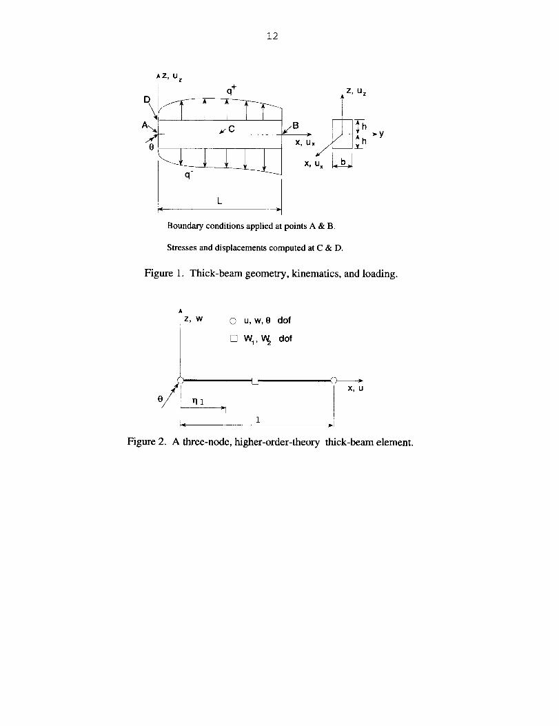
In this section a quasi-static Maxwell solid version of Tessler's 11 higher-order beam
theory is formulated and a simple beam finite element is derived. The beam dimensions and
sign convention are shown in Figure 1. The viscoelastic constitutive model for the beam
that is consistent with Eqs(16) and (17) can be written in matrix form as
N
and
S(t) : Ce+* C_ _ e(t)n=l
dne e de--'JC I'l __
dt "t"n dt
(18)
for each n. (19)
where
6
sT =(O'x.x, O'zz, "£xz)
eT ezz,rxz)
• r(. • .)n e = nExx, nl_zz, n_txz
["Cll Cl3 0
C =/C13 C33 0 and
Lo 0 C55
*C=
*Cll
*C13
*Cl3
*C3 3
0O],0
C55
where
- 14(h(3 - 5 2 ) 5(1-5 2 )hv135(4 752) _0z(5) = , Oxz(5)-
_0x(5) = 17 ' 17 4
The simplest finite element approximation of this beam theory, as explored in Ref. [ 11 ],
involves a three-node configuration (see Figure 2) which is achieved by the following
interpolations
u(rl, t ) = (1 - r/)u 0 (t) +/_U 1 (t) (25)
Wl(X,t) W2(X,t )g'zz -- + dPz (5) 2 + (Px (5) O(X,t),x (23)
h h
}txz =Oxz(5)(w(x,t), x +O(x,t)) (24)
where 5 = Z/h denotes a nondimensional thickness coordinate and 2h is the total
thickness. Note that u(x,t) represents the midplane (i.e. reference plane) axial
displacement, O(x, t) is the bending rotation of the cross-section of the beam, w(x, t) is
the weighted-average deflection, j_ and w I (x,t) and w2(x,t ) are the higher-order
transverse displacement variables enabling a parabolic distribution of u z (x, Z, t) through
the thickness. The above displacement assumptions give rise to the following thickness
distributions for the strains: a linear axial strain, a cubic transverse normal strain, and a
quadratic transverse shear strain, t_ These strain components have the following form
Cxx = u(x,t), x +hSO(x,t), x (22)
(21)
u x (x,z,t) = u(x,t) + hSO(x,t )
(x,z,t) = w(x,t) + 5wl (x,t) + (5U z\ 2 51) w2 (x,t)
(2O)
In this higher-order theory, the components of the displacement vector are approximated
through the beam thickness by way of five kinematic variables, i.e.,
7
o(_,t) --(1- ,;)Oo(0 +oo, It)x
w(r/, t)= (1 - r/)w 0 (t) + ?']W 1 (t)- _ 7"/(1-- r/)(0 0 (t)- 01 (t))
wl (rl, t) = Wl (t)
w2 (rl, t) = W2 (t)
where r] = x/1 is the nondimensional element length coordinate.
(26)
(27)
(28)
(29)
Note that the nodal
degrees-of-freedom at the two ends of the element are subscripted with indices 0 and 1.
Since the strains do not possess derivatives of the w 1(r/, t) and w 2 (r], t) variables,
these variables need not be continuous at the element nodes and, hence, their simplest
approximation is constant for each element. Their corresponding degrees-of-freedom are
attributed to a node at the element midspan.
For a quasi-static loading, the virtual work statement for an element of volume V
with the differential form of the Maxwell constitutive law included can be written as
N
I +EI =0 30)n=l
where the first integral represents the intemal virtual work done by the elastic stresses, the
second is the internal virtual work done by the viscous stresses, and _l/]/ is the virtual
work done by the external forces. Introducing Eqs(25)-(29) into Eqs(20)-(21) and
substituting the results into Eqs(22)-(24) yields finite element approximations of the strains
in terms of the nodal variables, i.e.,
e = Bu (31)
where
B
1 z 1 z0 0 0 - 0 -
i i i i
0 0 1 _qjx 1 qjz 0 0 Cx1 h h 2 1
o Cxz Cxz o o o Cxz _xz1 2 1 2
(32)
and u T : (u O, wo,O O, W 1, W2,Ul, W 1 ,01) denotes the element nodal displacement
vector.
A set of analogous nodal variables, n U, and corresponding viscous strains, n e, are
introduced. These are related by
8
ne=B nU
The virtual work statement for an element then becomes
N
u fB CBaV +E :- IB *cBdv :u- - on=l
By defining the integrals in Eq(34) as stiffness matrices, there results
N
E* T* *urk &l+ nu k Snu-_W =0n=l
Since Eq(19) irnplies_ =_2e when t is constant,
form
urk NE* T*-t- n u k t_u-t_W =0n=l
(33)
(34)
(35)
the virtual work takes on a simpler
This implies that at any given time the element equilibrium equations are
N
(36)
n=l
where f denotes the element consistent load vector due to the external loading.
Introducing Eqs(31) and (33) into the differential equations for the strain variables in
Eq(19) yields
dnu nU du-- + - for each n (38)
dt "¢n dt
The global equilibrium equations are determined by the standard assembly of the
element equations, Eqs(37). Note, there is no assembly for Eqs(38). The variables n U
are independent from element to element (recall, these variables carry the time dependent
information for the material within the element). The global equilibrium equations at a
given time are
Kug = Fmech - Fvisc (39)
where Ugdenotes the global nodal variable vector, K is the elastic stiffness matrix,
Fmech is the global force vector due to mechanical loads, and Fvisc is the assembled
N
vector for Z *k *u. The viscoelastic problem is solved by simultaneously integrating
n=l
ku+_*k *nU=f for each element (37)
the differential and algebraic equations expressed by Eqs(38) and (39), where the latter is
subject to the appropriate boundary restraints.
As far as the finite element implementation is concerned, a conventional linearly elastic
code can be readily adapted to perform the viscoelastic analysis for a Maxwell material,
i.e., for a material whose relaxation stiffness coefficients can be modeled with a Prony
series. First, the instantaneous stiffness coefficients, *Cijkl, are used in place of the elastic
values to compute the element viscous stiffness matrices, * k, which are stored for
>k
repeated use. The internal nodal variables for each element, n U, are set equal to their
initial values and stored. A predictor-corrector algorithm is then used to integrate Eqs(38)
and (39) in time. The predictor-corrector integration algorithm used in this effort is
described in the Appendix.
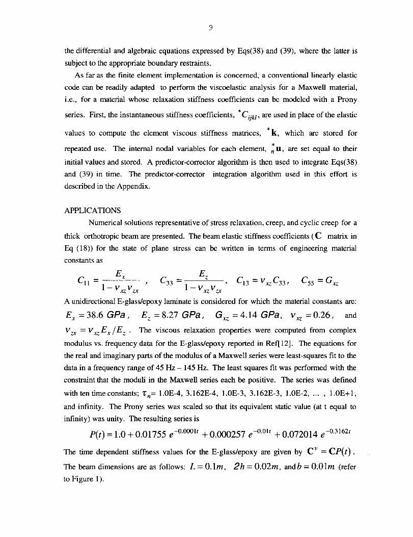
APPLICATIONS
Numerical solutions representative of stress relaxation, creep, and cyclic creep for a
thick orthotropic beam are presented. The beam elastic stiffness coefficients (C matrix in
Eq (18)) for the state of plane stress can be written in terms of engineering material
Ex E zCll = , C33 - , C13 -- VxzC33 , C55 = Gxz
1 - Vxz Vzx l - Vxz Vzx
A unidirectional E-glass/epoxy laminate is considered for which the material constants are:
E x=38.6 GPa, E z =8.27 GPa, Gxz =4.14 GPa, Vxz =0.26, and
Vzx = VxzE x/E z . The viscous relaxation properties were computed from complex
modulus vs. frequency data for the E-glass/epoxy reported in Ref[12]. The equations for
the real and imaginary parts of the modulus of a Maxwell series were least-squares fit to the
data in a frequency range of 45 Hz - 145 Hz. The least squares fit was performed with the
constraint that the moduli in the Maxwell series each be positive. The series was defined
with ten time constants; "t'n= 1.0E-4, 3.162E-4, 1.0E-3, 3.162E-3, 1.0E-2 ..... 1.0E+I,
and infinity. The Prony series was scaled so that its equivalent static value (at t equal to
infinity) was unity. The resulting series is
P(t) = 1.0 + 0.01755 e -°'°°°it + 0.000257 e -°'°it + 0.072014 e -0"3162/
The time dependent stiffness values for the E-glass/epoxy are given by C v = CP(t).
The beam dimensions are as follows: L = 0.1m, 2h = 0.02m, andb = 0.01m (refer
to Figure 1).
constants as
10
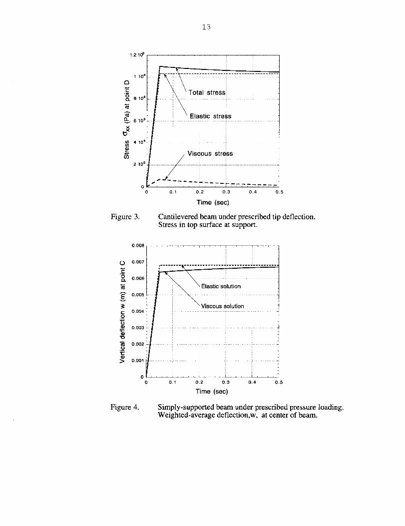
Example 1. A cantilever beam with w, u, 0 fixed at point A has a prescribed
deflection w at point B that is ramped from 0 to -1 cm in 0.05 sec and then held constant
at -1 cm. Figure 3 depicts the value of the maximum axial stress computed at point D as a
function of time. Also shown are the elastic and viscous stress components comprising the
total stress. The decay of the total viscoelastic stress to its elastic value as time is increased
demonstrates the expected step-strain relaxation behavior.
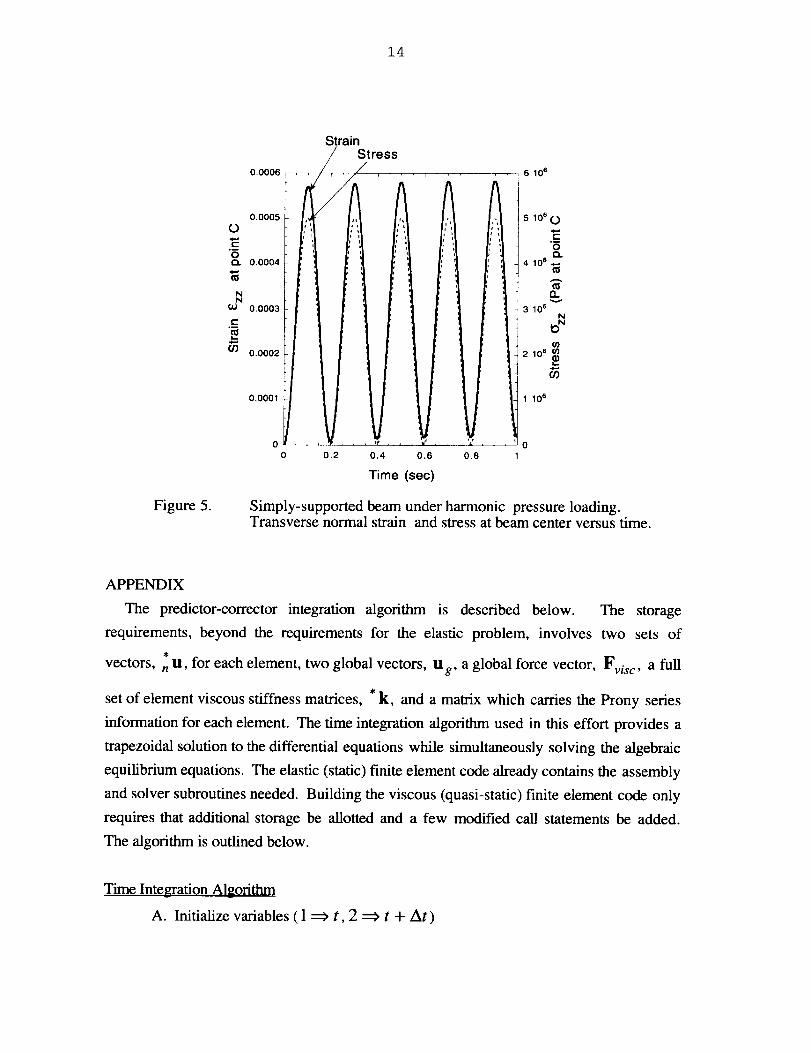
Example 2. A simply-supported beam with w and u fixed at point A and w fixed at
point B is subject to a uniform, top-surface pressure, q+ (t). The time-dependent value of
the pressure is ramped from 0.0 to 1.0 MPa in 0.05 sec and then held constant. Figure 4
shows the value of the w deflection at the midspan of the beam. The viscous solution
shows the expected creep response.
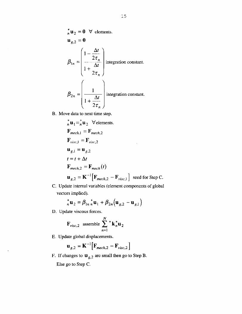
Example 3. The simply-supported beam in the preceding example is subject to a
harmonic pressure loading given by
q+(t) = 0, t < 0 and q+ (t) = 0.05 * (1 - COS(50Zrt)) MPa, t > 0
Figure 5 depicts the transverse normal stress and strain values at the midspan (point C)
versus time. The upward drift of the maximum and minimum values of the strain
demonstrates cyclic creep.
CONCLUSION
A differential form of the Maxwell viscous solid constitutive theory has been derived
and implemented within a higher-order-theory beam finite element. The finite element
formulation is attractive for several reasons: (1) The constitutive constants are the same as
those needed in the classical history-integral model, and they are also readily available from
step-strain relaxation tests, (2) The state variables are conjugate to the elastic strain
measures; hence, they are consistent with the kinematic assumptions of the elastic
formulation, (3) The update of the state variables can be performed in a parallel computing
environment, allowing the viscous force vector in the equations of motion to be determined
efficiently within the predictor-corrector algorithm, (4) Applications of time-dependent
displacements and loads are performed within the same finite element algorithm, and (5)
The higher-order beam theory accounts for both transverse shear and transverse normal
11
deformations-- theeffectsthat needto be accountedfor in thick and highly orthotropic
beams and high-frequency dynamics.
The computational examples for the problems of relaxation, creep, and cyclic creep
clearly demonstrated the predictive capabilities of the finite element formulation.
REFERENCES
1. Halpin, J. C., and Pagano, N. J., Observations on linear anisotropic viscoelasticity, J.
Composite Materials, 2, No. 1, 68-80 (1968).
2. Hashin, Z., Complex moduli of viscoelastic composites - I. General theory and
applications to particulate composites, Int. J. Solids Structures, 6, 539-552 (1970).
3. Hashin, Z., Complex moduli of viscoelastic composites - II. Fiber reinforced materials,
Int. J. Solids and Structures, 6, 797-807 (1970).
4. Argyris, J., St. Doltsinis, I., and daSilva, V. D., Constitutive modelling and
computation of non-linear viscoelastic solids, Part I. Rheological models and numerical
integration techniques, Comput. Methods Appl. Mech. Engrg., 88, 135-163 (1991).
5. Shaw, S., Warby, M. K., and Whiteman, J. R., Numerical techniques for problems of
quasistatic and dynamic viscoelasticity, in "The Mathematics of Finite Elements and
Applications," edited by J. R. Whiteman, John Wiley & Sons (1994).
6. Coleman, B. D., and Noll, W., Foundations of linear viscoelasticity, Reviews of
Modem Physics, 33, No.2, 239-249 (1961).
7. Schapery, R. A., Viscoelastic behavior and analysis of composite materials, in
"Composite Materials", 2, edited by G. P. Sendeckyj, Academic Press (1974).
8. Johnson, A. R., and Stacer, R. G., Rubber viscoelasticity using the physically
constrained system's stretches as internal variables, Rubber Chemistry and Technology,
66, No.4, 567-577 (1993).
9. Johnson, A. R., Tanner, J. A., and Mason, A. J., A kinematically driven anisotropic
viscoelastic constitutive model applied to tires, in "Computational Modeling of Tires,"
compiled by A. K. Noor and J. A. Tanner, NASA Conference Publication 3306, August
1995.
10. Johnson, A. R., Tanner, J. A., and Mason, J. A., A viscoelastic model for tires
analyzed with nonlinear shell elements, presented at the Fourteenth Annual Meeting and
Conference on Tire Science and Technology, University of Akron, March 1995.
11. Tessler, A., A two-node beam element including transverse shear and transverse
normal deformations, Int. J. for Numer. Methods Eng., 32, 1027-1039 (1991).
12. Gibson, R. F., and Plunkett, R., Dynamic mechanical behavior of fiber-reinforced
composites: Measurement and analysis, J. Composite Materials, 10, 325-341 (1976).
12
Z, U z
q+ z, uz
A-.
Xp U x
k L
q
Boundary conditions applied at points A & B.
Stresses and displacements computed at C & D.
Figure 1. Thick-beam geometry, kinematics, and loading.
Z, W 0 u,w,O dof
[] w,, _ dof
> X, U
nz
Figure 2. A three-node, higher-order-theory thick-beam element.
13
oo
Figure 3.
Total stressl
Elastic stress
Viscous stress
0.1 0.2 0.3 0.4 0.5
Time (sec)
Cantilevered beam under prescribed tip deflection.Stress in top surface at support.
oE"5Q..
Ev
t-O
.E
(9
B
"o
.o1_"
>
ooo8 t
0.007
0.006
0.005
0.004
0.003
0.002
O.O01
0
0
.... ] ...... I
i
i/ iiltiiii ill¸i :........ _-.... "......... -,......... , ........ -
0.1 0.2 0.3 0.4 0.5
Time (sec)
Figure 4. Simply-supported beam under prescribed pressure loading.Weighted-average deflection,w, at center of beam.
14
Figure5.
Strain/ Stress
0.0006 ....... 6 106
n
0.0005 II 5 108
"0_.. 0.0004 4 10s;
ra_ 0.0003 3 10 s N
0.0002 2 108
co
0.0001 1 106
0 0
0 0.2 0.4 0.6 0.8 1
Time (sec)
Simply-supported beam under harmonic pressure loading.Transverse normal strain and stress at beam center versus time.
APPENDIX
The predictor-corrector integration algorithm is described below. The storage
requirements, beyond the requirements for the elastic problem, involves two sets of
vectors, n U, for each element, two global vectors, u g, a global force vector, Fvisc, a full
set of element viscous stiffness matrices, * k, and a matrix which carries the Prony series
information for each element. The time integration algorithm used in this effort provides a
trapezoidal solution to the differential equations while simultaneously solving the algebraic
equilibrium equations. The elastic (static) finite element code already contains the assembly
and solver subroutines needed. Building the viscous (quasi-static) finite element code only
requires that additional storage be allotted and a few modified call statements be added.
The algorithm is outlined below.
Time Integration Algorithm
A. Initialize variables ( 1 =¢, t, 2 =:_ t + At)
3_5
nU2 =0
Ug,2 = 0
V elements.
Ii
_2n = / 1At1+--
2_" n
B. Move data to next time step.
n U 1 -- n U 2 V elements.
Fmech,l - Fmech,2
Fvisc,i = Fvisc,2
Ug,1 = Ug,2
t=t + At
integration constant.
integration constant.
Fmech,2 -- Fmech ( t )
Ug,2 -" K -1 [Fmech,2 - Fvisc,l ] seed for Step C.
C. Update internal variables (element components of global
vectors implied).
nU2 =J_ln -k-J_2n Ug,2 --Ug,1nal
D. Update viscous forces.
N
Fvisc,2 assemble Z * knU2n=l
E. Update global displacements.
Ug,2 -- K-l[Fmech,2 - Fvisc,2 ]
F. If changes to Ug,2 are small then go to Step B.
Else go to Step C.
REPORT DOCUMENTATION PAGE FormApprovedOMB No. 0704-0188
_ _. ,o.-mn_pnm_.p_ • .---.-__., -, _omlpmmg_, re'm,amg m_udin¢_b burckmest_me or anyothir ii_¢t of ttm
H_nway. um zo4,Amngto_VA 2_02-4302,andtot_eOIk:eclMaJw(lemmlandl__RMuclionPm/pct(0"/O_0188),_DC 20503.
1. AGENCY UeE ONLY (Leave b/ank) 2. REPORT DATE
June 1996
4. TITLE AND SIJa_; i LE 5. FUNDING NUMBERS
A Viscoelastic Higher-Order Beam Finite Element 505-63-53-01
e. AUTHOR(S)
Arthur R. Johnson and Alexander Tessler
7. PERFOR'--';;_k3 C.n36tANIZATION NAME(S) AND ADDRESS(B)
NASA Langley Research Center
Hampton, VA 23681-0001 and
Vehicle Structures Directorate
U.S. Army Research Laboratory
NASA Langley Research Center, Hampton, VA 23681-0001
9. spo_,_iNG / li,:,_n'ORm AGENCYNA_) ANDAOO_F.SS(EB)
National Aeronautics and Space AdministrationWashington, DC 20546-0001 andU.S. Army Research LaboratoryAdelphi, MD 20783-1145
_. RSJ_o,rrTVR ANo OATESCOVERB
Technical Memorandum
8. PERFORMING ORGANIZATIONREPORT NUMBER
lO. SPONSORING I MONITORINGAGENCY REPORT NUMBER
NASA TM- 110260ARL-MR-325
.. SUFeLE_NTANV_¥-=S
Paper presented at MAFELAP 1996, June 25-28, 1996, Uxbridge, United I_ngdom.
12L D_THi BUTION I AVAILABILITY STATEMENT
Unclassified- Unlimited
Subject Category 39
12b. DISTRIBUTION CODE
OF REPORT
UNCLASSIFIED
NSN 7540-01-280-5500
l& SECURITY C_iACATIONOF THIS PAGE
UNCLASSIFIED
!17. SECUFoT_ CLASSIFICATION
14. SUB,JF.CT TERMS
Viscoelasticity; Thick beams; Beam finite elements; and Maxwell Solid.
19. SECURITY CLASSIRCATIONOF ABSTRACT
UNCLASSIFIED
15. NUMBER OF PAGES
16
16. PRICE CODE
A03
20. UMIT&TION OF ABSTRACT
Standard Form 298 (Rev. 2-89)Pre_flbed byANSISKL Z30-182ge.-l_
13. Au._HACT (M_ 2_0 mx'cb)
A viscoelastic internal variable oonslimdve theory is applied to a higher-order elastic beam theory and finite element formulation. The
behavior of the viscous material in the beam is approximately modeled as a Maxwell solid. The finite element formulation requires
additional sets of nodal variables for each relaxali(m time constmu needed by the Maxwell solid. Recent developments in modeling
viscoelastic mau=ial behavic_ with strain variables that axe conjugate to the elastic strain measuzes are combined with advances in
modeling through-the-thickness stresses and strains in lttick beams. The result is a viscous fltick-beam finite element that possesses
superior characteristics f(x transient analysis since its nodal viscous forces _e not linearly dependent on the nodal velocities, which is the
case whe_ damping malrices &e used. Instead, ll_e nodal viscous forces are directly dependent on the mat_al's relaxation spectrum and
the history of the nodal variables through a differential form of the constitutive law for a Maxwell solid. The thick beam quasistatic
analysis is explored herein as a first step towards developing more c_nplex viscoelastic models for thick plates and shells, and for
dynamic enaly_s.
The internal variable constitutive theory is derived directly f_:nn the Bolt2mumn superposition theorem. The mechanical slzains and
the conjugate internal strains are shown to be related through a system of first-order, ordinm 3, differential equations. The total
lime-depender stress is the superposifio_ of its elastic and viscous comlxments. Equation,s of motion for the mlld are derived from the
virtual work principle using the toud lime-depeadent stre_s. Numerical examples for the problems of relaxation, creep, and cyclic creepare carried out for a besm m_d_ from an ortholronic Maxwell _lid.