1

VINS-Mono: A Robust and Versatile MonocularVisual-Inertial State Estimator

Tong Qin, Peiliang Li, and Shaojie Shen

Abstract—A monocular visual-inertial system (VINS), con-sisting of a camera and a low-cost inertial measurement unit(IMU), forms the minimum sensor suite for metric six degrees-of-freedom (DOF) state estimation. However, the lack of directdistance measurement poses significant challenges in terms ofIMU processing, estimator initialization, extrinsic calibration,and nonlinear optimization. In this work, we present VINS-Mono: a robust and versatile monocular visual-inertial stateestimator. Our approach starts with a robust procedure forestimator initialization and failure recovery. A tightly-coupled,nonlinear optimization-based method is used to obtain highaccuracy visual-inertial odometry by fusing pre-integrated IMUmeasurements and feature observations. A loop detection module,in combination with our tightly-coupled formulation, enablesrelocalization with minimum computation overhead. We addi-tionally perform four degrees-of-freedom pose graph optimiza-tion to enforce global consistency. We validate the performanceof our system on public datasets and real-world experimentsand compare against other state-of-the-art algorithms. We alsoperform onboard closed-loop autonomous flight on the MAVplatform and port the algorithm to an iOS-based demonstration.We highlight that the proposed work is a reliable, complete,and versatile system that is applicable for different applicationsthat require high accuracy localization. We open source ourimplementations for both PCs1 and iOS mobile devices2.

Index Terms—Monocular visual-inertial systems, state estima-tion, sensor fusion, simultaneous localization and mapping

I. INTRODUCTION

STATE estimation is undoubtedly the most fundamentalmodule for a wide range of applications, such as robotic

navigation, autonomous driving, virtual reality (VR), andaugmented reality (AR). Approaches that use only a monocularcamera have gained significant interests by the community dueto their small size, low-cost, and easy hardware setup [1]–[5]. However, monocular vision-only systems are incapable ofrecovering the metric scale, therefore limiting their usage inreal-world robotic applications. Recently, we see a growingtrend of assisting the monocular vision system with a low-cost inertial measurement unit (IMU). The primary advantageof this monocular visual-inertial system (VINS) is to havethe metric scale, as well as roll and pitch angles, all observ-able. This enables navigation tasks that require metric stateestimates. In addition, the integration of IMU measurementscan dramatically improve motion tracking performance bybridging the gap between losses of visual tracks due to

T. Qin, P. Li, and S. Shen are with the Department of Electronic andComputer Engineering, Hong Kong University of Science and Technology.e-mail: tqinab, pliap@connect.ust.hk, eeshaojie@ust.hk

1https://github.com/HKUST-Aerial-Robotics/VINS-Mono2https://github.com/HKUST-Aerial-Robotics/VINS-Mobile

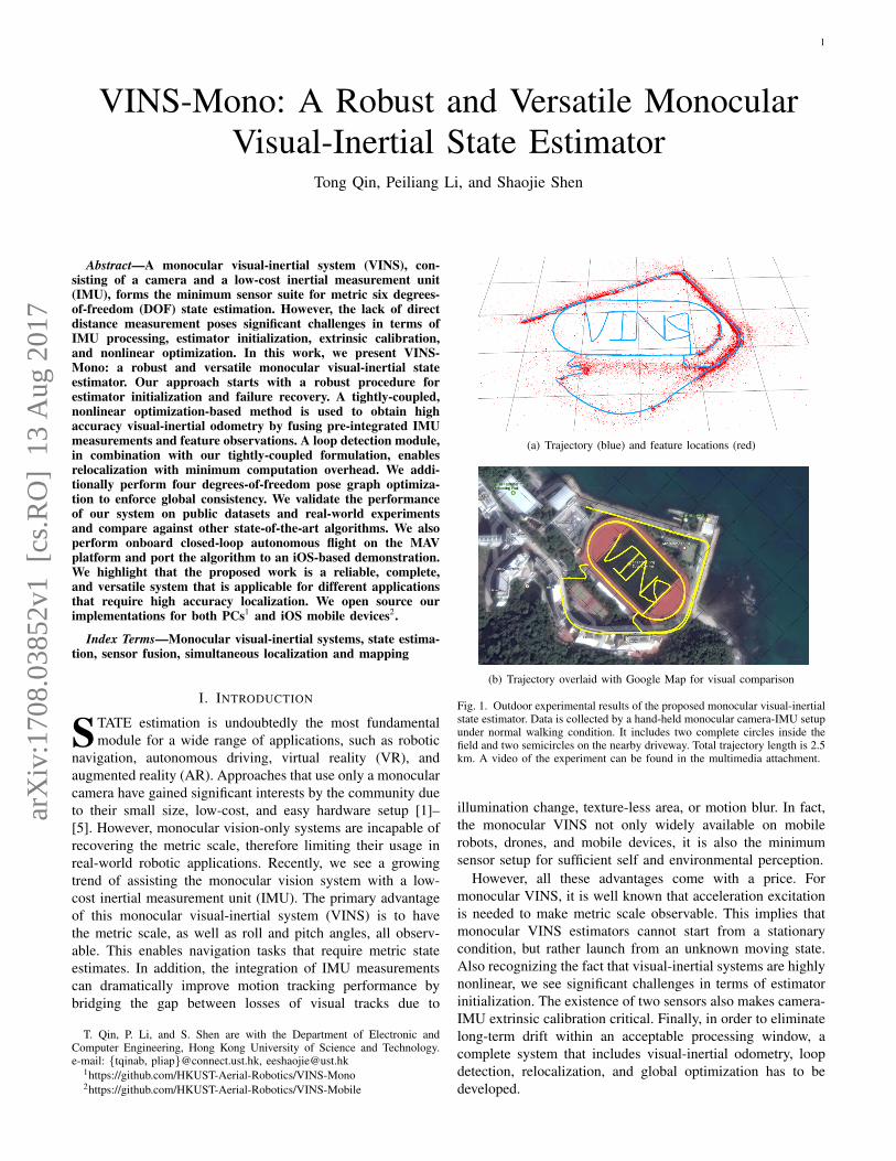
(a) Trajectory (blue) and feature locations (red)

(b) Trajectory overlaid with Google Map for visual comparison

Fig. 1. Outdoor experimental results of the proposed monocular visual-inertialstate estimator. Data is collected by a hand-held monocular camera-IMU setupunder normal walking condition. It includes two complete circles inside thefield and two semicircles on the nearby driveway. Total trajectory length is 2.5km. A video of the experiment can be found in the multimedia attachment.

illumination change, texture-less area, or motion blur. In fact,the monocular VINS not only widely available on mobilerobots, drones, and mobile devices, it is also the minimumsensor setup for sufficient self and environmental perception.

However, all these advantages come with a price. Formonocular VINS, it is well known that acceleration excitationis needed to make metric scale observable. This implies thatmonocular VINS estimators cannot start from a stationarycondition, but rather launch from an unknown moving state.Also recognizing the fact that visual-inertial systems are highlynonlinear, we see significant challenges in terms of estimatorinitialization. The existence of two sensors also makes camera-IMU extrinsic calibration critical. Finally, in order to eliminatelong-term drift within an acceptable processing window, acomplete system that includes visual-inertial odometry, loopdetection, relocalization, and global optimization has to bedeveloped.

arX

iv:1

708.

0385

2v1

[cs

.RO

] 1

3 A

ug 2

017

2

To address all these issues, we propose VINS-Mono, arobust and versatile monocular visual-inertial state estimator.Our solution starts with on-the-fly estimator initialization. Thesame initialization module is also used for failure recovery.The core of our solution is a robust monocular visual-inertialodometry (VIO) based on tightly-coupled sliding window non-linear optimization. The monocular VIO module not only pro-vides accurate local pose, velocity, and orientation estimates,it also performs camera-IMU extrinsic calibration and IMUbiases correction in an online fashion. Loops are detected usingDBoW2 [6]. Relocalization is done in a tightly-coupled settingby feature-level fusion with the monocular VIO. This enablesrobust and accurate relocalization with minimum computationoverhead. Finally, geometrically verified loops are added into apose graph, and thanks to the observable roll and pitch anglesfrom the monocular VIO, a four degrees-of-freedom (DOF)pose graph is performed to ensure global consistency.

VINS-Mono combines and improves the our previous workson monocular visual-inertial fusion [7]–[10]. It is built ontop our tightly-coupled, optimization-based formulation formonocular VIO [7], [8], and incorporates the improved ini-tialization procedure introduced in [9]. The first attempt ofporting to mobile devices was given in [10]. Further im-provements of VINS-Mono comparing to our previous worksinclude improved IMU pre-integration with bias correction,tightly-coupled relocalization, global pose graph optimization,extensive experimental evaluation, and a robust and versatileopen source implementation.

The whole system is complete and easy-to-use. It has beensuccessfully applied to small-scale AR scenarios, medium-scale drone navigation, and large-scale state estimation tasks.Superior performance has been shown against other state-of-the-art methods. To this end, we summarize our contributionsas follow:

• A robust initialization procedure that is able to bootstrapthe system from unknown initial states.

• A tightly-coupled, optimization-based monocular visual-inertial odometry with camera-IMU extrinsic calibrationand IMU bias estimation.

• Online loop detection and tightly-coupled relocalization.• Four DOF global pose graph optimization.• Real-time performance demonstration for drone naviga-

tion, large-scale localization, and mobile AR applications.• Open-source release for both the PC version that is fully

integrated with ROS, as well as the iOS version that runson iPhone6s or above.

The rest of the paper is structured as follows. In Sect. II,we discuss relevant literature. We give an overview of thecomplete system pipeline in Sect. III. Preprocessing stepsfor both visual and pre-integrated IMU measurements arepresented in Sect. IV. In Sect. V, we discuss the estimatorinitialization procedure. A tightly-coupled, self-calibrating,nonlinear optimization-based monocular VIO, is presentedin Sect. VI. Tightly-coupled relocalization and global posegraph optimization are presented in Sect. VII and Sect. VIIIrespectively. Implementation details and experimental resultsare shown in Sect. IX. Finally, the paper is concluded with a

discussion and possible future research directions in Sect. X.

II. RELATED WORK

Scholarly works on monocular vision-based state estima-tion/odometry/SLAM are extensive. Noticeable approachesinclude PTAM [1], SVO [2], LSD-SLAM [3], DSO [5], andORB-SLAM [4]. It is obvious that any attempts to give a fullrelevant review would be incomplete. In this section, however,we skip the discussion on vision-only approaches, and onlyfocus on the most relevant results on monocular visual-inertialstate estimation.

The simplest way to deal with visual and inertial mea-surements is loosely-coupled sensor fusion [11], [12], whereIMU is treated as an independent module to assist vision-onlypose estimates obtained from the visual structure from motion.Fusion is usually done by an extended Kalman filter (EKF),where IMU is used for state propagation and the vision-onlypose is used for the update. Further on, tightly-coupled visual-inertial algorithms are either based on the EKF [13]–[15] orgraph optimization [7], [8], [16], [17], where camera and IMUmeasurements are jointly optimized from the raw measurementlevel. A popular EKF based VIO approach is MSCKF [13],[14]. MSCKF maintains several previous camera poses in thestate vector, and uses visual measurements of the same featureacross multiple camera views to form multi-constraint update.SR-ISWF [18], [19] is an extension of MSCKF. It uses square-root form [20] to achieve single-precision representation andavoid poor numerical properties. This approach employs theinverse filter for iterative re-linearization, making it equalto optimization-based algorithms. Batch graph optimizationor bundle adjustment techniques maintain and optimize allmeasurements to obtain the optimal state estimates. To achieveconstant processing time, popular graph-based VIO meth-ods [8], [16], [17] usually optimize over a bounded-size slidingwindow of recent states by marginalizing out past states andmeasurements. Due to high computational demands of iterativesolving of nonlinear systems, few graph-based can achievereal-time performance on resource-constrained platforms, suchas mobile phones.

For visual measurement processing, algorithms can be cat-egorized into either direct or indirect method according tothe definition of visual residual models. Direct approaches[2], [3], [21] minimize photometric error while indirect ap-proaches [8], [14], [16] minimize geometric displacement.Direct methods require a good initial guess due to their smallregion of attraction, while indirect approaches consume extracomputational resources on extracting and matching features.Indirect approaches are more frequently found in real-worldengineering deployment due to its maturity and robustness.However, direct approaches are easier to be extended for densemapping as they are operated directly on the pixel level.

In practice, IMUs usually acquire data at a much higher ratethan the camera. Different methods have been proposed to han-dle the high rate IMU measurements. The most straightforwardapproach is to use the IMU for state propagation in EKF-basedapproaches [11], [13]. In a graph optimization formulation, anefficient technique called IMU pre-integration is developed in

3

+$/ '6

'6 /$(,1$&/ 1(-,

$ 12/$$1$"1(-, ,#/ ")(,&(0(-,-,*5

%(02 *(,$/1( **(&,+$,1

,(1( *(6$# $0*(#(,&(,#-4 $4$01*#$01 .1(+(6 1(-,

! 0$#

$5%/ +$ 1 ! 0$

--. $1$"1$#1 1$0%/-+--.*-02/$

*-! *-0$/ .'.1(+(6 1(-,$"1

$5%/ +$

,(1( *(6 1(-,$"1$ 02/$+$,1/$./-"$00(,&$"1

-" *(02 *(,$/1( *#-+$1/54(1'$*-" *(6 1(-,$"1

$ 12/$$1/($3 *$0

--0$/ .'.1(+(6 1(-,

$0

/ 1$-0$

+$/ / 1$-0$

/-. & 1(-,

-1(-,

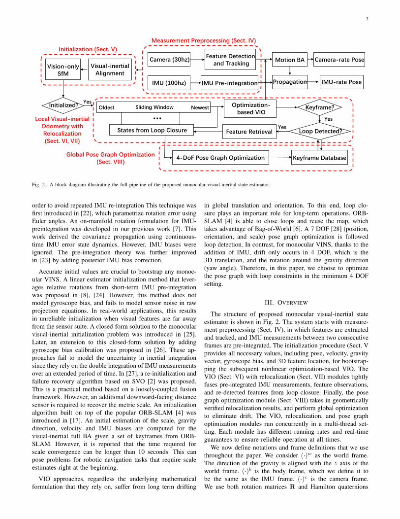
Fig. 2. A block diagram illustrating the full pipeline of the proposed monocular visual-inertial state estimator.

order to avoid repeated IMU re-integration This technique wasfirst introduced in [22], which parametrize rotation error usingEuler angles. An on-manifold rotation formulation for IMU-preintegration was developed in our previous work [7]. Thiswork derived the covariance propagation using continuous-time IMU error state dynamics. However, IMU biases wereignored. The pre-integration theory was further improvedin [23] by adding posterior IMU bias correction.

Accurate initial values are crucial to bootstrap any monoc-ular VINS. A linear estimator initialization method that lever-ages relative rotations from short-term IMU pre-integrationwas proposed in [8], [24]. However, this method does notmodel gyroscope bias, and fails to model sensor noise in rawprojection equations. In real-world applications, this resultsin unreliable initialization when visual features are far awayfrom the sensor suite. A closed-form solution to the monocularvisual-inertial initialization problem was introduced in [25].Later, an extension to this closed-form solution by addinggyroscope bias calibration was proposed in [26]. These ap-proaches fail to model the uncertainty in inertial integrationsince they rely on the double integration of IMU measurementsover an extended period of time. In [27], a re-initialization andfailure recovery algorithm based on SVO [2] was proposed.This is a practical method based on a loosely-coupled fusionframework. However, an additional downward-facing distancesensor is required to recover the metric scale. An initializationalgorithm built on top of the popular ORB-SLAM [4] wasintroduced in [17]. An initial estimation of the scale, gravitydirection, velocity and IMU biases are computed for thevisual-inertial full BA given a set of keyframes from ORB-SLAM. However, it is reported that the time required forscale convergence can be longer than 10 seconds. This canpose problems for robotic navigation tasks that require scaleestimates right at the beginning.

VIO approaches, regardless the underlying mathematicalformulation that they rely on, suffer from long term drifting

in global translation and orientation. To this end, loop clo-sure plays an important role for long-term operations. ORB-SLAM [4] is able to close loops and reuse the map, whichtakes advantage of Bag-of-World [6]. A 7 DOF [28] (position,orientation, and scale) pose graph optimization is followedloop detection. In contrast, for monocular VINS, thanks to theaddition of IMU, drift only occurs in 4 DOF, which is the3D translation, and the rotation around the gravity direction(yaw angle). Therefore, in this paper, we choose to optimizethe pose graph with loop constraints in the minimum 4 DOFsetting.

III. OVERVIEW

The structure of proposed monocular visual-inertial stateestimator is shown in Fig. 2. The system starts with measure-ment preprocessing (Sect. IV), in which features are extractedand tracked, and IMU measurements between two consecutiveframes are pre-integrated. The initialization procedure (Sect. Vprovides all necessary values, including pose, velocity, gravityvector, gyroscope bias, and 3D feature location, for bootstrap-ping the subsequent nonlinear optimization-based VIO. TheVIO (Sect. VI) with relocalization (Sect. VII) modules tightlyfuses pre-integrated IMU measurements, feature observations,and re-detected features from loop closure. Finally, the posegraph optimization module (Sect. VIII) takes in geometricallyverified relocalization results, and perform global optimizationto eliminate drift. The VIO, relocalization, and pose graphoptimization modules run concurrently in a multi-thread set-ting. Each module has different running rates and real-timeguarantees to ensure reliable operation at all times.

We now define notations and frame definitions that we usethroughout the paper. We consider (·)w as the world frame.The direction of the gravity is aligned with the z axis of theworld frame. (·)b is the body frame, which we define it tobe the same as the IMU frame. (·)c is the camera frame.We use both rotation matrices R and Hamilton quaternions

4

q to represent rotation. We primarily use quaternions in statevectors, but rotation matrices are also used for conveniencerotation of 3D vectors. qwb ,p

wb are rotation and translation

from the body frame to the world frame. bk is the bodyframe while taking the kth image. ck is the camera framewhile taking the kth image. ⊗ represents the multiplicationoperation between two quaternions. gw = [0, 0, g]T is thegravity vector in the world frame. Finally, we denote (·) asthe noisy measurement or estimate of a certain quantity.

IV. MEASUREMENT PREPROCESSING

This section presents preprocessing steps for both inertialand monocular visual measurements. For visual measurements,we track features between consecutive frames and detect newfeatures in the latest frame. For IMU measurements, we pre-integrate them between two consecutive frames. Note that themeasurements of the low-cost IMU that we use are affectedby both bias and noise. We therefore especially take bias intoaccount in the IMU pre-integration process.

A. Vision Processing Front-end

For each new image, existing features are tracked by theKLT sparse optical flow algorithm [29]. Meanwhile, new cor-ner features are detected [30] to maintain a minimum number(100-300) of features in each image. The detector enforces auniform feature distribution by setting a minimum separationof pixels between two neighboring features. 2D Features arefirstly undistorted and then projected to a unit sphere afterpassing outlier rejection. Outlier rejection is performed usingRANSAC with fundamental matrix model [31].

Keyframes are also selected in this step. We have two crite-ria for keyframe selection. The first one is the average parallaxapart from the previous keyframe. If the average parallax oftracked features is between the current frame and the latestkeyframe is beyond a certain threshold, we treat frame as anew keyframe. Note that not only translation but also rotationcan cause parallax. However, features cannot be triangulated inthe rotation-only motion. To avoid this situation, we use short-term integration of gyroscope measurements to compensaterotation when calculating parallax. Note that this rotationcompensation is only used to keyframe selection, and is notinvolved in rotation calculation in the VINS formulation. Tothis end, even if the gyroscope contains large noise or is biased,it will only result in suboptimal keyframe selection results,and will not directly affect the estimation quality. Anothercriterion is tracking quality. If the number of tracked featuresgoes below a certain threshold, we treat this frame as a newkeyframe. This criterion is to avoid complete loss of featuretracks.

B. IMU Pre-integration

IMU Pre-integration was first proposed in [22], whichparametrized rotation error in Euler angle. An on-manifoldrotation formulation for IMU pre-integration was developedin our previous work [7]. This work derived the covariancepropagation using continuous-time IMU error state dynamics.

However, IMU biases were ignored. The pre-integration theorywas further improved in [23] by adding posterior IMU biascorrection. In this paper, we extend the IMU pre-integrationproposed in our previous work [7] by incorporating IMU biascorrection.

The raw gyroscope and accelerometer measurements fromIMU, ω and a, are given by:

at = at + bat + Rtwgw + na

ωt = ωt + bwt+ nw.

(1)

IMU measurements, which are measured in the body frame,combines the force for countering gravity and the platformdynamics, and are affected by acceleration bias ba, gyroscopebias bw, and additive noise. We assume that the additive noisein acceleration and gyroscope measurements are Gaussian,na ∼ N (0,σ2

a), nw ∼ N (0,σ2w). Acceleration bias and

gyroscope bias are modeled as random walk, whose derivativesare Gaussian, nba ∼ N (0,σ2

ba), nbw ∼ N (0,σ2

bw):

bat = nba , bwt= nbw . (2)

Given two time instants that correspond to image framesbk and bk+1, position, velocity, and orientation states canbe propagated by inertial measurements during time interval[tk, tk+1] in the world frame:

pwbk+1= pwbk + vwbk∆tk

+

∫∫t∈[tk,tk+1]

(Rwt (at − bat − na)− gw) dt2

vwbk+1= vwbk +

∫t∈[tk,tk+1]

(Rwt (at − bat − na)− gw) dt

qwbk+1= qwbk ⊗

∫t∈[tk,tk+1]

1

2Ω(ωt − bwt

− nw)qbkt dt,

(3)

where

Ω(ω) =

[−bωc× ω−ωT 0

], bωc× =

0 −ωz ωyωz 0 −ωx−ωy ωx 0

.(4)

∆tk is the duration between the time interval [tk, tk+1].It can be seen that the IMU state propagation requires

rotation, position and velocity of frame bk. When these startingstates change, we need to re-propagate IMU measurements.Especially in the optimization-based algorithm, every time weadjust poses, we will need to re-propagate IMU measurementsbetween them. This propagation strategy is computationallydemanding. To avoid re-propagation, we adopt pre-integrationalgorithm.

After change the reference frame from the world frame tothe local frame bk, we can only pre-integrate the parts whichare related to linear acceleration a and angular velocity ω asfollows:

Rbkw pwbk+1

= Rbkw (pwbk + vwbk∆tk −

1

2gw∆t2k) +αbkbk+1

Rbkw vwbk+1

= Rbkw (vwbk − gw∆tk) + βbkbk+1

qbkw ⊗ qwbk+1= γbkbk+1

,

(5)

5

x"x# x$

x%

f#f'

x'

f$f"

x(' x(" x(#

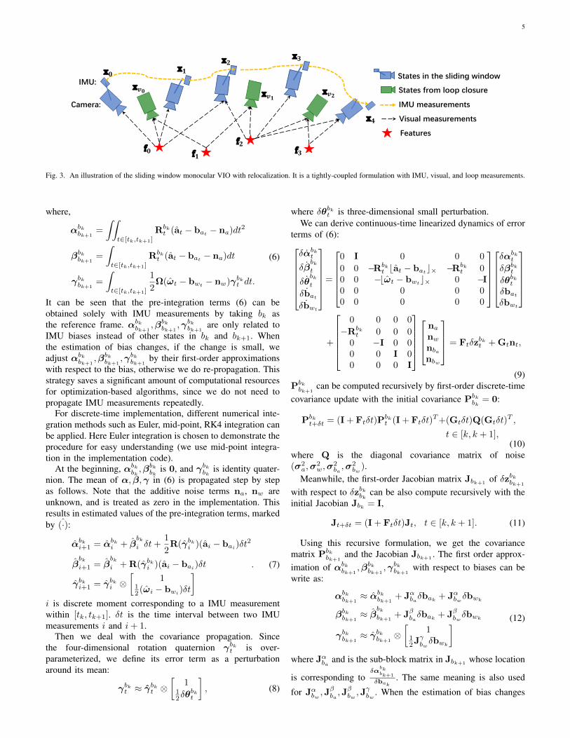
Fig. 3. An illustration of the sliding window monocular VIO with relocalization. It is a tightly-coupled formulation with IMU, visual, and loop measurements.

where,

αbkbk+1=

∫∫t∈[tk,tk+1]

Rbkt (at − bat − na)dt2

βbkbk+1=

∫t∈[tk,tk+1]

Rbkt (at − bat − na)dt

γbkbk+1=

∫t∈[tk,tk+1]

1

2Ω(ωt − bwt

− nw)γbkt dt.

(6)

It can be seen that the pre-integration terms (6) can beobtained solely with IMU measurements by taking bk asthe reference frame. αbkbk+1

,βbkbk+1,γbkbk+1

are only related toIMU biases instead of other states in bk and bk+1. Whenthe estimation of bias changes, if the change is small, weadjust αbkbk+1

,βbkbk+1,γbkbk+1

by their first-order approximationswith respect to the bias, otherwise we do re-propagation. Thisstrategy saves a significant amount of computational resourcesfor optimization-based algorithms, since we do not need topropagate IMU measurements repeatedly.

For discrete-time implementation, different numerical inte-gration methods such as Euler, mid-point, RK4 integration canbe applied. Here Euler integration is chosen to demonstrate theprocedure for easy understanding (we use mid-point integra-tion in the implementation code).

At the beginning, αbkbk ,βbkbk

is 0, and γbkbk is identity quater-nion. The mean of α,β,γ in (6) is propagated step by stepas follows. Note that the additive noise terms na, nw areunknown, and is treated as zero in the implementation. Thisresults in estimated values of the pre-integration terms, markedby (·):

αbki+1 = αbki + βbki δt+

1

2R(γbki )(ai − bai)δt

2

βbki+1 = β

bki + R(γbki )(ai − bai)δt

γbki+1 = γbki ⊗[

112 (ωi − bwi)δt

] . (7)

i is discrete moment corresponding to a IMU measurementwithin [tk, tk+1]. δt is the time interval between two IMUmeasurements i and i+ 1.

Then we deal with the covariance propagation. Sincethe four-dimensional rotation quaternion γbkt is over-parameterized, we define its error term as a perturbationaround its mean:

γbkt ≈ γbkt ⊗

[1

12δθ

bkt

], (8)

where δθbkt is three-dimensional small perturbation.We can derive continuous-time linearized dynamics of error

terms of (6):δαbkt

δβbkt

δθbkt

δbatδbwt

=

0 I 0 0 0

0 0 −Rbkt bat − batc× −Rbk

t 00 0 −bωt − bwt

c× 0 −I0 0 0 0 00 0 0 0 0

δαbktδβbktδθbktδbatδbwt

+

0 0 0 0

−Rbkt 0 0 0

0 −I 0 00 0 I 00 0 0 I

nanwnbanbw

= Ftδzbkt + Gtnt,

(9)Pbkbk+1

can be computed recursively by first-order discrete-timecovariance update with the initial covariance Pbk

bk= 0:

Pbkt+δt = (I + Ftδt)P

bkt (I + Ftδt)

T+(Gtδt)Q(Gtδt)T ,

t ∈ [k, k + 1],(10)

where Q is the diagonal covariance matrix of noise(σ2

a,σ2w,σ

2ba,σ2

bw).

Meanwhile, the first-order Jacobian matrix Jbk+1of δzbkbk+1

with respect to δzbkbk can be also compute recursively with theinitial Jacobian Jbk = I,

Jt+δt = (I + Ftδt)Jt, t ∈ [k, k + 1]. (11)

Using this recursive formulation, we get the covariancematrix Pbk

bk+1and the Jacobian Jbk+1

. The first order approx-imation of αbkbk+1

,βbkbk+1,γbkbk+1

with respect to biases can bewrite as:

αbkbk+1≈ αbkbk+1

+ Jαbaδbak + Jαbwδbwk

βbkbk+1≈ β

bkbk+1

+ Jβbaδbak + Jβbwδbwk

γbkbk+1≈ γbkbk+1

⊗[

112Jγbwδbwk

] (12)

where Jαba and is the sub-block matrix in Jbk+1whose location

is corresponding toδα

bkbk+1

δbak. The same meaning is also used

for Jαbw ,Jβba,Jβbw ,J

γbw

. When the estimation of bias changes

6

Fig. 4. An illustration of the visual-inertial alignment process for estimatorinitialization.

slightly, we use (12) to correct pre-integration results approx-imately instead of re-propagation.

Now we are able to write down the IMU measurementmodel with its corresponding covariance Pbk

bk+1:

αbkbk+1

βbkbk+1

γbkbk+1

00

=

Rbkw (pwbk+1

− pwbk + 12gw∆t2k − vwbk∆tk)

Rbkw (vwbk+1

+ gw∆tk − vwbk)

qw−1

bk⊗ qwbk+1

babk+1− babk

bwbk+1− bwbk

.(13)

V. ESTIMATOR INITIALIZATION

Monocular tightly-coupled visual-inertial odometry is ahighly nonlinear system. Since the scale is not directly ob-servable from a monocular camera, it is hard to directly fusethese two measurements without good initial values. One mayassume a stationary initial condition to start the monocularVINS estimator. However, this assumption is inappropriateas initialization under motion is frequently encountered inreal-world applications. The situation becomes even morecomplicated when IMU measurements are corrupted by largebias. In fact, initialization is usually the most fragile step formonocular VINS. A robust initialization procedure is neededto ensure the applicability of the system.

We adopt a loosely-coupled sensor fusion method to getinitial values. We find that vision-only SLAM, or Structurefrom Motion (SfM), has a good property of initialization.In most cases, a visual-only system can bootstrap itself byderived initial values from relative motion methods, such asthe eight-point [32] or five-point [33] algorithms, or estimatingthe homogeneous matrices. By aligning metric IMU pre-integration with the visual-only SfM results, we can roughlyrecover scale, gravity, velocity, and even bias. This is sufficientfor bootstrapping a nonlinear monocular VINS estimator, asshown in Fig. 4.

In contrast to [17], which simultaneously estimates gyro-scope and accelerometer bias during the initialization phase,we choose to ignore accelerometer bias terms in the initialstep. Accelerometer bias is coupled with gravity, and due to thelarge magnitude of the gravity vector comparing to platformdynamics, and the relatively short during of the initializationphase, these bias terms are hard to be observed. A detailedanalysis of accelerometer bias calibration is presented in ourprevious work [34].

A. Sliding Window Vision-Only SfM

The initialization procedure starts with a vision-only SfMto estimate a graph of up-to-scale camera poses and featurepositions.

We maintain a sliding window of frames for boundedcomputational complexity. Firstly, we check feature correspon-dences between the latest frame and all previous frames. If wecan find stable feature tracking (more than 30 tracked features)and sufficient parallax (more than 20 rotation-compensatedpixels) between the latest frame and any other frames in thesliding window. we recover the relative rotation and up-to-scale translation between these two frames using the Five-pointalgorithm [33]. Otherwise, we keep the latest frame in thewindow and wait for new frames. If the five-point algorithmsuccess, we arbitrarily set the scale and triangulate all featuresobserved in these two frames. Based on these triangulatedfeatures, a perspective-n-point (PnP) method [35] is performedto estimate poses of all other frames in the window. Finally,a global full bundle adjustment [36] is applied to minimizethe total reprojection error of all feature observations. Sincewe do not yet have any knowledge about the world frame,we set the first camera frame (·)c0 as the reference framefor SfM. All frame poses (pc0ck ,qc0ck ) and feature positions arerepresented with respect to (·)c0 . Suppose we have a roughmeasure extrinsic parameters (pbc,q

bc) between the camera and

the IMU, we can translate poses from camera frame to body(IMU) frame,

qc0bk = qc0ck ⊗ (qbc)−1

spc0bk = spc0ck −Rc0bk

pbc,(14)

where s the scaling parameter that aligns the visual structureto the metric scale. Solving this scaling parameter is the keyto achieve successful initialization.

B. Visual-Inertial Alignment

1) Gyroscope Bias Calibration: Consider two consecutiveframes bk and bk+1 in the window, we get the rotation qc0bk andqc0bk+1

from the visual SfM, as well as the relative constraintγbkbk+1

from IMU pre-integration. We linearize the IMU pre-integration term with respect to gyroscope bias and minimizethe following cost function:

minδbw

∑k∈B

∥∥∥qc0bk+1

−1⊗ qc0bk ⊗ γbkbk+1

∥∥∥2γbkbk+1

≈ γbkbk+1⊗[

112Jγbwδbw

],

(15)

where B indexes all frames in the window. We have the firstorder approximation of γbkbk+1

with respect to the gyroscopebias using the bias Jacobian derived in Sect. IV-B. In such way,we get an initial calibration of the gyroscope bias bw. Thenwe re-propagate all IMU pre-integration terms αbkbk+1

, βbkbk+1

,and γbkbk+1

using the new gyroscope bias.2) Velocity, Gravity Vector and Metric Scale Initialization:

After the gyroscope bias is initialized, we move on to initialize

7

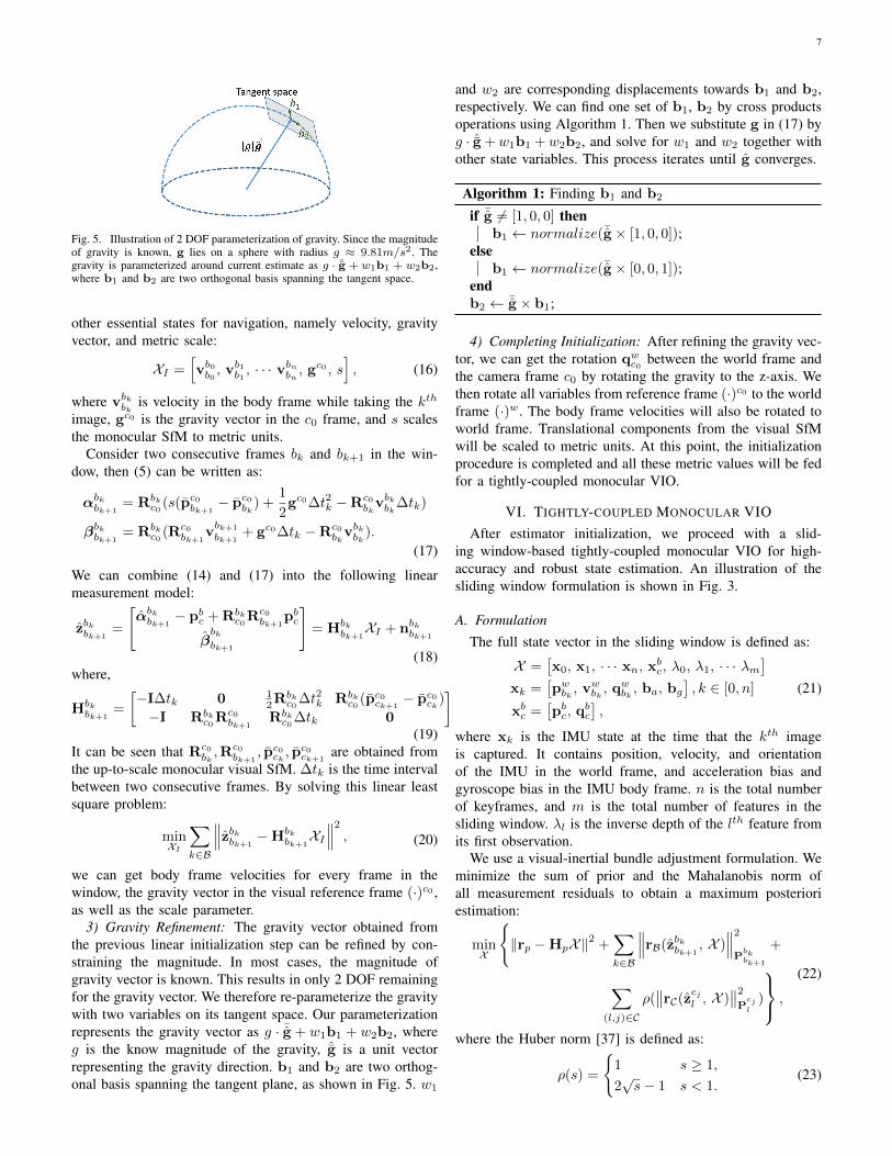
Fig. 5. Illustration of 2 DOF parameterization of gravity. Since the magnitudeof gravity is known, g lies on a sphere with radius g ≈ 9.81m/s2. Thegravity is parameterized around current estimate as g · ˆg + w1b1 + w2b2,where b1 and b2 are two orthogonal basis spanning the tangent space.

other essential states for navigation, namely velocity, gravityvector, and metric scale:

XI =[vb0b0 , vb1b1 , · · · v

bnbn, gc0 , s

], (16)

where vbkbk is velocity in the body frame while taking the kth

image, gc0 is the gravity vector in the c0 frame, and s scalesthe monocular SfM to metric units.

Consider two consecutive frames bk and bk+1 in the win-dow, then (5) can be written as:

αbkbk+1= Rbk

c0 (s(pc0bk+1− pc0bk) +

1

2gc0∆t2k −Rc0

bkvbkbk∆tk)

βbkbk+1= Rbk

c0 (Rc0bk+1

vbk+1

bk+1+ gc0∆tk −Rc0

bkvbkbk ).

(17)

We can combine (14) and (17) into the following linearmeasurement model:

zbkbk+1=

[αbkbk+1

− pbc + Rbkc0Rc0

bk+1pbc

βbkbk+1

]= Hbk

bk+1XI + nbkbk+1

(18)where,

Hbkbk+1

=

[−I∆tk 0 1

2Rbkc0 ∆t2k Rbk

c0 (pc0ck+1− pc0ck)

−I Rbkc0Rc0

bk+1Rbkc0 ∆tk 0

](19)

It can be seen that Rc0bk,Rc0

bk+1, pc0ck , p

c0ck+1

are obtained fromthe up-to-scale monocular visual SfM. ∆tk is the time intervalbetween two consecutive frames. By solving this linear leastsquare problem:

minXI

∑k∈B

∥∥∥zbkbk+1−Hbk

bk+1XI∥∥∥2 , (20)

we can get body frame velocities for every frame in thewindow, the gravity vector in the visual reference frame (·)c0 ,as well as the scale parameter.

3) Gravity Refinement: The gravity vector obtained fromthe previous linear initialization step can be refined by con-straining the magnitude. In most cases, the magnitude ofgravity vector is known. This results in only 2 DOF remainingfor the gravity vector. We therefore re-parameterize the gravitywith two variables on its tangent space. Our parameterizationrepresents the gravity vector as g · ¯g + w1b1 + w2b2, whereg is the know magnitude of the gravity, ˆg is a unit vectorrepresenting the gravity direction. b1 and b2 are two orthog-onal basis spanning the tangent plane, as shown in Fig. 5. w1

and w2 are corresponding displacements towards b1 and b2,respectively. We can find one set of b1, b2 by cross productsoperations using Algorithm 1. Then we substitute g in (17) byg · ˆg +w1b1 +w2b2, and solve for w1 and w2 together withother state variables. This process iterates until g converges.

Algorithm 1: Finding b1 and b2

if ¯g 6= [1, 0, 0] thenb1 ← normalize(¯g × [1, 0, 0]);

elseb1 ← normalize(¯g × [0, 0, 1]);

endb2 ← ¯g × b1;

4) Completing Initialization: After refining the gravity vec-tor, we can get the rotation qwc0 between the world frame andthe camera frame c0 by rotating the gravity to the z-axis. Wethen rotate all variables from reference frame (·)c0 to the worldframe (·)w. The body frame velocities will also be rotated toworld frame. Translational components from the visual SfMwill be scaled to metric units. At this point, the initializationprocedure is completed and all these metric values will be fedfor a tightly-coupled monocular VIO.

VI. TIGHTLY-COUPLED MONOCULAR VIOAfter estimator initialization, we proceed with a slid-

ing window-based tightly-coupled monocular VIO for high-accuracy and robust state estimation. An illustration of thesliding window formulation is shown in Fig. 3.

A. FormulationThe full state vector in the sliding window is defined as:

X =[x0, x1, · · · xn, xbc, λ0, λ1, · · · λm

]xk =

[pwbk , vwbk , qwbk , ba, bg

], k ∈ [0, n]

xbc =[pbc, qbc

],

(21)

where xk is the IMU state at the time that the kth imageis captured. It contains position, velocity, and orientationof the IMU in the world frame, and acceleration bias andgyroscope bias in the IMU body frame. n is the total numberof keyframes, and m is the total number of features in thesliding window. λl is the inverse depth of the lth feature fromits first observation.

We use a visual-inertial bundle adjustment formulation. Weminimize the sum of prior and the Mahalanobis norm ofall measurement residuals to obtain a maximum posterioriestimation:

minX

‖rp −HpX‖2 +

∑k∈B

∥∥∥rB(zbkbk+1, X )

∥∥∥2P

bkbk+1

+

∑(l,j)∈C

ρ(∥∥rC(zcjl , X )

∥∥2P

cjl

)

,

(22)

where the Huber norm [37] is defined as:

ρ(s) =

1 s ≥ 1,

2√s− 1 s < 1.

(23)

8

rB(zbkbk+1, X ) and rC(z

cjl , X ) are residuals for IMU and visual

measurements respectively. Detailed definition of the residualterms will be presented in Sect. VI-B and Sect. VI-C. B is theset of all IMU measurements, C is the set of features whichhave been observed at least twice in the current sliding win-dow. rp, Hp is the prior information from marginalization.Ceres Solver [38] is used for solving this nonlinear problem.

B. IMU Measurement Residual

Consider the IMU measurements within two consecutiveframes bk and bk+1 in the sliding window, according to theIMU measurement model defined in (13), the residual for pre-integrated IMU measurement can be defined as:

rB(zbkbk+1, X ) =

δαbkbk+1

δβbkbk+1

δθbkbk+1

δbaδbg

=

Rbkw (pwbk+1

− pwbk + 12gw∆t2k − vwbk∆tk)− αbkbk+1

Rbkw (vwbk+1

+ gw∆tk − vwbk)− βbkbk+1

2[qw

−1

bk⊗ qwbk+1

⊗ (γbkbk+1)−1]xyz

babk+1− babk

bwbk+1− bwbk

,(24)

where[·]xyz

extracts the vector part of a quaternion q for errorstate representation. δθbkbk+1

is the three dimensional error-

state representation of quaternion. [αbkbk+1, β

bkbk+1

, γbkbk+1]T are

pre-integrated IMU measurement terms using only noisy ac-celerometer and gyroscope measurements within the time in-terval between two consecutive image frames. Accelerometerand gyroscope biases are also included in the residual termsfor online correction.

C. Visual Measurement Residual

In contrast to traditional pinhole camera models that definereprojection errors on a generalized image plane, we definethe camera measurement residual on a unit sphere. The opticsfor almost all types of cameras, including wide-angle, fisheyeor omnidirectional cameras, can be modeled as a unit rayconnecting the surface of a unit sphere. Consider the lth

feature that is first observed in the ith image, the residualfor the feature observation in the jth image is defined as:

rC(zcjl , X ) =

[b1 b2

]T · ( ˆPcjl −Pcjl‖Pcjl ‖

)

ˆPcjl = πc−1

(

[ucjl

vcjl

])

Pcjl = Rcb(R

bjw (Rw

bi(Rbc

1

λlπc

−1(

[ucilvcil

])

+ pbc) + pwbi − pwbj )− pbc),

(25)

where [ucil , vcil ] is the first observation of the lth feature that

happens in the ith image. [ucjl , v

cjl ] is the observation of the

Tangent plane

Unit sphere

!"

#$"%

||#$"%||

#'$"%

()*+

*,

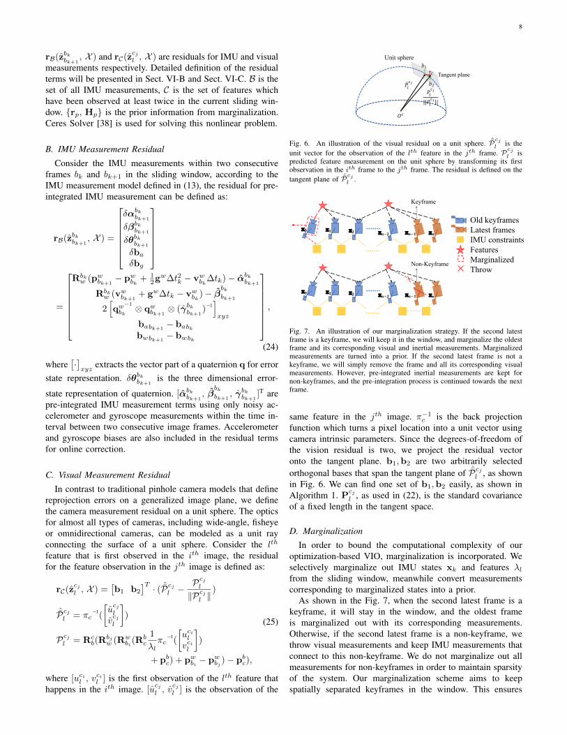
Fig. 6. An illustration of the visual residual on a unit sphere. ˆPcjl is the

unit vector for the observation of the lth feature in the jth frame. Pcjl is

predicted feature measurement on the unit sphere by transforming its firstobservation in the ith frame to the jth frame. The residual is defined on thetangent plane of ˆPcj

l .

Old keyframesLatest framesIMU constraintsFeaturesMarginalizedThrow

Keyframe

x" x# x$ x%&#x%&$ x%

Non-Keyframe

x" x# x$ x%&#x%&$ x%

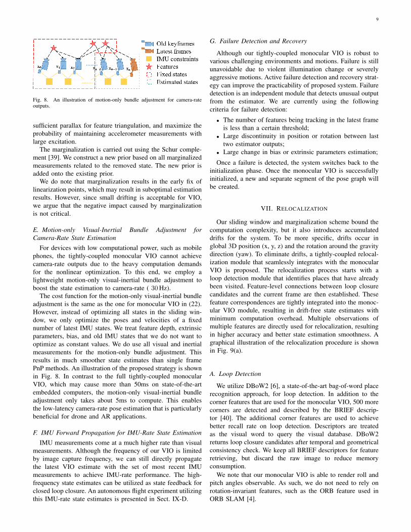
Fig. 7. An illustration of our marginalization strategy. If the second latestframe is a keyframe, we will keep it in the window, and marginalize the oldestframe and its corresponding visual and inertial measurements. Marginalizedmeasurements are turned into a prior. If the second latest frame is not akeyframe, we will simply remove the frame and all its corresponding visualmeasurements. However, pre-integrated inertial measurements are kept fornon-keyframes, and the pre-integration process is continued towards the nextframe.

same feature in the jth image. π−1c is the back projectionfunction which turns a pixel location into a unit vector usingcamera intrinsic parameters. Since the degrees-of-freedom ofthe vision residual is two, we project the residual vectoronto the tangent plane. b1,b2 are two arbitrarily selectedorthogonal bases that span the tangent plane of ˆPcjl , as shownin Fig. 6. We can find one set of b1,b2 easily, as shown inAlgorithm 1. P

cjl , as used in (22), is the standard covariance

of a fixed length in the tangent space.

D. Marginalization

In order to bound the computational complexity of ouroptimization-based VIO, marginalization is incorporated. Weselectively marginalize out IMU states xk and features λlfrom the sliding window, meanwhile convert measurementscorresponding to marginalized states into a prior.

As shown in the Fig. 7, when the second latest frame is akeyframe, it will stay in the window, and the oldest frameis marginalized out with its corresponding measurements.Otherwise, if the second latest frame is a non-keyframe, wethrow visual measurements and keep IMU measurements thatconnect to this non-keyframe. We do not marginalize out allmeasurements for non-keyframes in order to maintain sparsityof the system. Our marginalization scheme aims to keepspatially separated keyframes in the window. This ensures

9

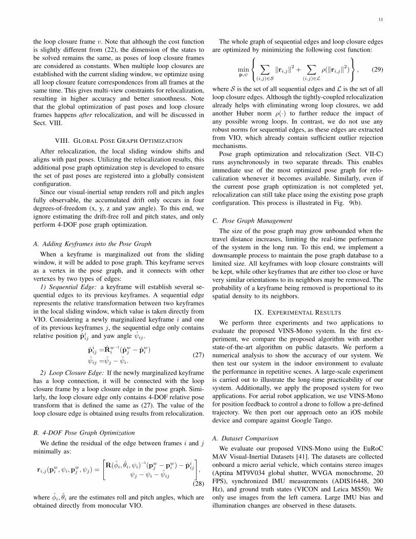
Fig. 8. An illustration of motion-only bundle adjustment for camera-rateoutputs.

sufficient parallax for feature triangulation, and maximize theprobability of maintaining accelerometer measurements withlarge excitation.

The marginalization is carried out using the Schur comple-ment [39]. We construct a new prior based on all marginalizedmeasurements related to the removed state. The new prior isadded onto the existing prior.

We do note that marginalization results in the early fix oflinearization points, which may result in suboptimal estimationresults. However, since small drifting is acceptable for VIO,we argue that the negative impact caused by marginalizationis not critical.

E. Motion-only Visual-Inertial Bundle Adjustment forCamera-Rate State Estimation

For devices with low computational power, such as mobilephones, the tightly-coupled monocular VIO cannot achievecamera-rate outputs due to the heavy computation demandsfor the nonlinear optimization. To this end, we employ alightweight motion-only visual-inertial bundle adjustment toboost the state estimation to camera-rate ( 30 Hz).

The cost function for the motion-only visual-inertial bundleadjustment is the same as the one for monocular VIO in (22).However, instead of optimizing all states in the sliding win-dow, we only optimize the poses and velocities of a fixednumber of latest IMU states. We treat feature depth, extrinsicparameters, bias, and old IMU states that we do not want tooptimize as constant values. We do use all visual and inertialmeasurements for the motion-only bundle adjustment. Thisresults in much smoother state estimates than single framePnP methods. An illustration of the proposed strategy is shownin Fig. 8. In contrast to the full tightly-coupled monocularVIO, which may cause more than 50ms on state-of-the-artembedded computers, the motion-only visual-inertial bundleadjustment only takes about 5ms to compute. This enablesthe low-latency camera-rate pose estimation that is particularlybeneficial for drone and AR applications.

F. IMU Forward Propagation for IMU-Rate State Estimation

IMU measurements come at a much higher rate than visualmeasurements. Although the frequency of our VIO is limitedby image capture frequency, we can still directly propagatethe latest VIO estimate with the set of most recent IMUmeasurements to achieve IMU-rate performance. The high-frequency state estimates can be utilized as state feedback forclosed loop closure. An autonomous flight experiment utilizingthis IMU-rate state estimates is presented in Sect. IX-D.

G. Failure Detection and Recovery

Although our tightly-coupled monocular VIO is robust tovarious challenging environments and motions. Failure is stillunavoidable due to violent illumination change or severelyaggressive motions. Active failure detection and recovery strat-egy can improve the practicability of proposed system. Failuredetection is an independent module that detects unusual outputfrom the estimator. We are currently using the followingcriteria for failure detection:

• The number of features being tracking in the latest frameis less than a certain threshold;

• Large discontinuity in position or rotation between lasttwo estimator outputs;

• Large change in bias or extrinsic parameters estimation;

Once a failure is detected, the system switches back to theinitialization phase. Once the monocular VIO is successfullyinitialized, a new and separate segment of the pose graph willbe created.

VII. RELOCALIZATION

Our sliding window and marginalization scheme bound thecomputation complexity, but it also introduces accumulateddrifts for the system. To be more specific, drifts occur inglobal 3D position (x, y, z) and the rotation around the gravitydirection (yaw). To eliminate drifts, a tightly-coupled relocal-ization module that seamlessly integrates with the monocularVIO is proposed. The relocalization process starts with aloop detection module that identifies places that have alreadybeen visited. Feature-level connections between loop closurecandidates and the current frame are then established. Thesefeature correspondences are tightly integrated into the monoc-ular VIO module, resulting in drift-free state estimates withminimum computation overhead. Multiple observations ofmultiple features are directly used for relocalization, resultingin higher accuracy and better state estimation smoothness. Agraphical illustration of the relocalization procedure is shownin Fig. 9(a).

A. Loop Detection

We utilize DBoW2 [6], a state-of-the-art bag-of-word placerecognition approach, for loop detection. In addition to thecorner features that are used for the monocular VIO, 500 morecorners are detected and described by the BRIEF descrip-tor [40]. The additional corner features are used to achievebetter recall rate on loop detection. Descriptors are treatedas the visual word to query the visual database. DBoW2returns loop closure candidates after temporal and geometricalconsistency check. We keep all BRIEF descriptors for featureretrieving, but discard the raw image to reduce memoryconsumption.

We note that our monocular VIO is able to render roll andpitch angles observable. As such, we do not need to rely onrotation-invariant features, such as the ORB feature used inORB SLAM [4].

10

1. Visual-Inertial Odometry 2. Loop Detection 3. Relocalization

4. Relocalization with Multiple Constraints

(a) Relocalization

5. Add Keyframe into Pose Graph

6. 4-DoF Pose GraphOptimization

7. Relocalization inOptimized Pose Graph

Keyframes in databaseKeyframes in Window Sequential links

Loop links

Window links

Marginalized Keyframe

(b) Global Pose Graph optimization

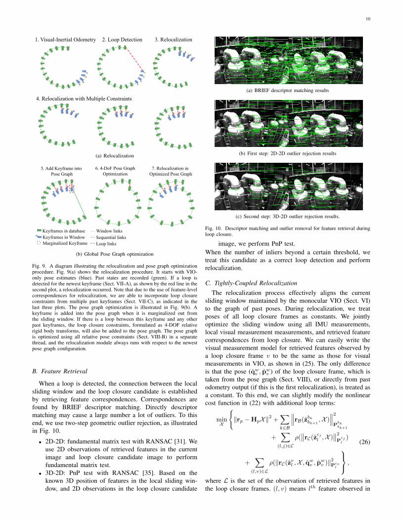
Fig. 9. A diagram illustrating the relocalization and pose graph optimizationprocedure. Fig. 9(a) shows the relocalization procedure. It starts with VIO-only pose estimates (blue). Past states are recorded (green). If a loop isdetected for the newest keyframe (Sect. VII-A), as shown by the red line in thesecond plot, a relocalization occurred. Note that due to the use of feature-levelcorrespondences for relocalization, we are able to incorporate loop closureconstraints from multiple past keyframes (Sect. VII-C), as indicated in thelast three plots. The pose graph optimization is illustrated in Fig. 9(b). Akeyframe is added into the pose graph when it is marginalized out fromthe sliding window. If there is a loop between this keyframe and any otherpast keyframes, the loop closure constraints, formulated as 4-DOF relativerigid body transforms, will also be added to the pose graph. The pose graphis optimized using all relative pose constraints (Sect. VIII-B) in a separatethread, and the relocalization module always runs with respect to the newestpose graph configuration.

B. Feature Retrieval

When a loop is detected, the connection between the localsliding window and the loop closure candidate is establishedby retrieving feature correspondences. Correspondences arefound by BRIEF descriptor matching. Directly descriptormatching may cause a large number a lot of outliers. To thisend, we use two-step geometric outlier rejection, as illustratedin Fig. 10.

• 2D-2D: fundamental matrix test with RANSAC [31]. Weuse 2D observations of retrieved features in the currentimage and loop closure candidate image to performfundamental matrix test.

• 3D-2D: PnP test with RANSAC [35]. Based on theknown 3D position of features in the local sliding win-dow, and 2D observations in the loop closure candidate

(a) BRIEF descriptor matching results

(b) First step: 2D-2D outlier rejection results

(c) Second step: 3D-2D outlier rejection results.

Fig. 10. Descriptor matching and outlier removal for feature retrieval duringloop closure.

image, we perform PnP test.When the number of inliers beyond a certain threshold, wetreat this candidate as a correct loop detection and performrelocalization.

C. Tightly-Coupled RelocalizationThe relocalization process effectively aligns the current

sliding window maintained by the monocular VIO (Sect. VI)to the graph of past poses. During relocalization, we treatposes of all loop closure frames as constants. We jointlyoptimize the sliding window using all IMU measurements,local visual measurement measurements, and retrieved featurecorrespondences from loop closure. We can easily write thevisual measurement model for retrieved features observed bya loop closure frame v to be the same as those for visualmeasurements in VIO, as shown in (25). The only differenceis that the pose (qwv , p

wv ) of the loop closure frame, which is

taken from the pose graph (Sect. VIII), or directly from pastodometry output (if this is the first relocalization), is treated asa constant. To this end, we can slightly modify the nonlinearcost function in (22) with additional loop terms:

minX

‖rp −HpX‖2 +

∑k∈B

∥∥∥rB(zbkbk+1,X )

∥∥∥2P

bkbk+1

+∑

(l,j)∈C

ρ(∥∥rC(zcjl ,X )

∥∥2P

cjl

)

+∑

(l,v)∈L

ρ(‖rC(zvl ,X , qwv , pwv )‖2Pcvl

,

(26)

where L is the set of the observation of retrieved features inthe loop closure frames. (l, v) means lth feature observed in

11

the loop closure frame v. Note that although the cost functionis slightly different from (22), the dimension of the states tobe solved remains the same, as poses of loop closure framesare considered as constants. When multiple loop closures areestablished with the current sliding window, we optimize usingall loop closure feature correspondences from all frames at thesame time. This gives multi-view constraints for relocalization,resulting in higher accuracy and better smoothness. Notethat the global optimization of past poses and loop closureframes happens after relocalization, and will be discussed inSect. VIII.

VIII. GLOBAL POSE GRAPH OPTIMIZATION

After relocalization, the local sliding window shifts andaligns with past poses. Utilizing the relocalization results, thisadditional pose graph optimization step is developed to ensurethe set of past poses are registered into a globally consistentconfiguration.

Since our visual-inertial setup renders roll and pitch anglesfully observable, the accumulated drift only occurs in fourdegrees-of-freedom (x, y, z and yaw angle). To this end, weignore estimating the drift-free roll and pitch states, and onlyperform 4-DOF pose graph optimization.

A. Adding Keyframes into the Pose Graph

When a keyframe is marginalized out from the slidingwindow, it will be added to pose graph. This keyframe servesas a vertex in the pose graph, and it connects with othervertexes by two types of edges:

1) Sequential Edge: a keyframe will establish several se-quential edges to its previous keyframes. A sequential edgerepresents the relative transformation between two keyframesin the local sliding window, which value is taken directly fromVIO. Considering a newly marginalized keyframe i and oneof its previous keyframes j, the sequential edge only containsrelative position piij and yaw angle ψij .

piij =Rwi

−1(pwj − pwi )

ψij =ψj − ψi.(27)

2) Loop Closure Edge: If the newly marginalized keyframehas a loop connection, it will be connected with the loopclosure frame by a loop closure edge in the pose graph. Simi-larly, the loop closure edge only contains 4-DOF relative posetransform that is defined the same as (27). The value of theloop closure edge is obtained using results from relocalization.

B. 4-DOF Pose Graph Optimization

We define the residual of the edge between frames i and jminimally as:

ri,j(pwi , ψi,p

wj , ψj) =

[R(φi, θi, ψi)

−1(pwj − pwi )− piij

ψj − ψi − ψij

],

(28)

where φi, θi are the estimates roll and pitch angles, which areobtained directly from monocular VIO.

The whole graph of sequential edges and loop closure edgesare optimized by minimizing the following cost function:

minp,ψ

∑(i,j)∈S

‖ri,j‖2 +∑

(i,j)∈L

ρ(‖ri,j‖2)

, (29)

where S is the set of all sequential edges and L is the set of allloop closure edges. Although the tightly-coupled relocalizationalready helps with eliminating wrong loop closures, we addanother Huber norm ρ(·) to further reduce the impact ofany possible wrong loops. In contrast, we do not use anyrobust norms for sequential edges, as these edges are extractedfrom VIO, which already contain sufficient outlier rejectionmechanisms.

Pose graph optimization and relocalization (Sect. VII-C)runs asynchronously in two separate threads. This enablesimmediate use of the most optimized pose graph for relo-calization whenever it becomes available. Similarly, even ifthe current pose graph optimization is not completed yet,relocalization can still take place using the existing pose graphconfiguration. This process is illustrated in Fig. 9(b).

C. Pose Graph Management

The size of the pose graph may grow unbounded when thetravel distance increases, limiting the real-time performanceof the system in the long run. To this end, we implement adownsample process to maintain the pose graph database to alimited size. All keyframes with loop closure constraints willbe kept, while other keyframes that are either too close or havevery similar orientations to its neighbors may be removed. Theprobability of a keyframe being removed is proportional to itsspatial density to its neighbors.

IX. EXPERIMENTAL RESULTS

We perform three experiments and two applications toevaluate the proposed VINS-Mono system. In the first ex-periment, we compare the proposed algorithm with anotherstate-of-the-art algorithm on public datasets. We perform anumerical analysis to show the accuracy of our system. Wethen test our system in the indoor environment to evaluatethe performance in repetitive scenes. A large-scale experimentis carried out to illustrate the long-time practicability of oursystem. Additionally, we apply the proposed system for twoapplications. For aerial robot application, we use VINS-Monofor position feedback to control a drone to follow a pre-definedtrajectory. We then port our approach onto an iOS mobiledevice and compare against Google Tango.

A. Dataset Comparison

We evaluate our proposed VINS-Mono using the EuRoCMAV Visual-Inertial Datasets [41]. The datasets are collectedonboard a micro aerial vehicle, which contains stereo images(Aptina MT9V034 global shutter, WVGA monochrome, 20FPS), synchronized IMU measurements (ADIS16448, 200Hz), and ground truth states (VICON and Leica MS50). Weonly use images from the left camera. Large IMU bias andillumination changes are observed in these datasets.

12

x [m]-2 0 2 4 6 8 10 12 14

y [m

]

-4

-2

0

2

4

6

8Trajectory in MH_03_median

VINSVINS_loopOKVIS_monoOKVIS_stereoGroud Truth

Fig. 11. Trajectory in MH 03 median, compared with OKVIS.

time [s]0 20 40 60 80 100 120 140

x er

ror [

m]

0

0.5

1Error in MH_03_median

VINSVINS_loopOKVIS_monoOKVIS_stereo

time [s]0 20 40 60 80 100 120 140

y er

ror [

m]

0

0.5

1

1.5

time [s]0 20 40 60 80 100 120 140

z er

ror [

m]

00.10.20.30.4

distance [m]0 20 40 60 80 100 120 140Tr

anla

tion

erro

r [m

]

0

0.5

1

1.5

Fig. 12. Translation error plot in MH 03 median.

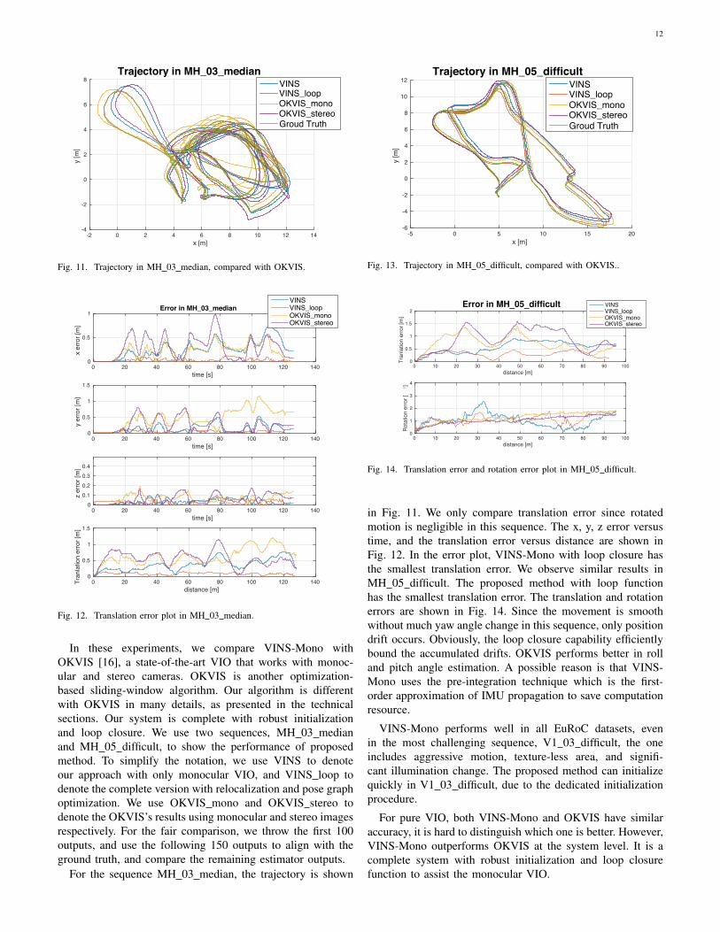
In these experiments, we compare VINS-Mono withOKVIS [16], a state-of-the-art VIO that works with monoc-ular and stereo cameras. OKVIS is another optimization-based sliding-window algorithm. Our algorithm is differentwith OKVIS in many details, as presented in the technicalsections. Our system is complete with robust initializationand loop closure. We use two sequences, MH 03 medianand MH 05 difficult, to show the performance of proposedmethod. To simplify the notation, we use VINS to denoteour approach with only monocular VIO, and VINS loop todenote the complete version with relocalization and pose graphoptimization. We use OKVIS mono and OKVIS stereo todenote the OKVIS’s results using monocular and stereo imagesrespectively. For the fair comparison, we throw the first 100outputs, and use the following 150 outputs to align with theground truth, and compare the remaining estimator outputs.

For the sequence MH 03 median, the trajectory is shown

x [m]-5 0 5 10 15 20

y [m

]

-6

-4

-2

0

2

4

6

8

10

12Trajectory in MH_05_difficult

VINSVINS_loopOKVIS_monoOKVIS_stereoGroud Truth

Fig. 13. Trajectory in MH 05 difficult, compared with OKVIS..

distance [m]

0 10 20 30 40 50 60 70 80 90 100

Tra

nla

tio

n e

rro

r [m

]

0

0.5

1

1.5

2Error in MH_05_difficult VINS

VINS_loopOKVIS_monoOKVIS_stereo

distance [m]

0 10 20 30 40 50 60 70 80 90 100

Ro

tatio

n e

rro

r [

°]

0

1

2

3

4

Fig. 14. Translation error and rotation error plot in MH 05 difficult.

in Fig. 11. We only compare translation error since rotatedmotion is negligible in this sequence. The x, y, z error versustime, and the translation error versus distance are shown inFig. 12. In the error plot, VINS-Mono with loop closure hasthe smallest translation error. We observe similar results inMH 05 difficult. The proposed method with loop functionhas the smallest translation error. The translation and rotationerrors are shown in Fig. 14. Since the movement is smoothwithout much yaw angle change in this sequence, only positiondrift occurs. Obviously, the loop closure capability efficientlybound the accumulated drifts. OKVIS performs better in rolland pitch angle estimation. A possible reason is that VINS-Mono uses the pre-integration technique which is the first-order approximation of IMU propagation to save computationresource.

VINS-Mono performs well in all EuRoC datasets, evenin the most challenging sequence, V1 03 difficult, the oneincludes aggressive motion, texture-less area, and signifi-cant illumination change. The proposed method can initializequickly in V1 03 difficult, due to the dedicated initializationprocedure.

For pure VIO, both VINS-Mono and OKVIS have similaraccuracy, it is hard to distinguish which one is better. However,VINS-Mono outperforms OKVIS at the system level. It is acomplete system with robust initialization and loop closurefunction to assist the monocular VIO.

13

Fig. 15. The device we used for the indoor experiment. It containsone forward-looking global shutter camera (MatrixVision mvBlueFOX-MLC200w) with 752×480 resolution. We use the built-in IMU (ADXL278and ADXRS290, 100Hz) for the DJI A3 flight controller.

(a) Pedestrians (b) texture-less area

(c) Low light condition (d) Glass and reflection

Fig. 16. Sample images for the challenging indoor experiment.

B. Indoor Experiment

In the indoor experiment, we choose our laboratory environ-ment as the experiment area. The sensor suite we use is shownin Fig. 15. It contains a monocular camera (20Hz) and an IMU(100Hz) inside the DJI A3 controller3. We hold the sensorsuite by hand and walk in normal pace in the laboratory. Weencounter pedestrians, low light condition, texture-less area,glass and reflection, as shown in Fig. 16. Videos can be foundin the multimedia attachment.

We compare our result with OKVIS, as shown in Fig. 17.Fig. 17(a) is the VIO output from OKVIS. Fig. 17(b) is theVIO-only result from proposed method without loop closure.Fig. 17(c) is the result of the proposed method with relocal-ization and loop closure. Noticeable VIO drifts occurred whenwe circle indoor. Both OKVIS and the VIO-only version ofVINS-Mono accumulate significant drifts in x, y, z, and yawangle. Our relocalization and loop closure modules efficientlyeliminate all these drifts.

C. Large-scale Environment

1) Go out of the lab: We test VINS-Mono in a mixedindoor and outdoor setting. The sensor suite is the same as the

3http://www.dji.com/a3

(a) Trajectory of OKVIS. (b) Trajectory of VINS-Mono with-out loop closure.

(c) Trajectory of VINS-Mono withrelocalization and loop closure. Redlines indicate loop detection.

Fig. 17. Results of the indoor experiment with comparison against OKVIS.

one shown in Fig. 15. We started from a seat in the laboratoryand go around the indoor space. Then we went down thestairs and walked around the playground outside the building.Next, we went back to the building and go upstairs. Finally,we returned to the same seat in the laboratory. The wholetrajectory is more than 700 meters and last approximatelyten minutes. A video of the experiment can be found in themultimedia attachment.

The trajectory is shown in Fig. 19. Fig. 19(a) is the trajectoryfrom OKVIS. When we went up stairs, OKVIS shows unstablefeature tracking, resulting in bad estimation. We cannot seethe shape of stairs in the red block. The VIO-only result fromVINS-Mono is shown in Fig. 19(b). The trajectory with loopclosure is shown in Fig. 19(c). The shape of stairs is clear inproposed method. The closed loop trajectory is aligned withGoogle Map to verify its accuracy, as shown in Fig. 18.

The final drift for OKVIS is [13.80, -5.26. 7.23]m in x, yand z-axis. The final dirft of VINS-Mono without loop closureis [-5.47, 2.76. -0.29]m, which occupies 0.88% with respect tothe total trajectory length, smaller than OKVIS 2.36%. Withloop correction. the final drift is bounded to [-0.032, 0.09, -0.07]m, which is trivial compared to the total trajectory length.Although we do not have ground truth, we can still visuallyinspect that the optimized trajectory is smooth and can beprecisely aligned with the satellite map.

2) Go around campus: This very large-scale dataset thatgoes around the whole HKUST campus was recorded witha handheld VI-Sensor4. The dataset covers the ground that isaround 710m in length, 240m in width, and with 60m in heightchanges. The total path length is 5.62km. The data containsthe 25Hz image and 200Hz IMU lasting for 1 hour and 34

4http://www.skybotix.com/

14

Fig. 18. The estimated trajectory of the mixed indoor and outdoor experimentaligned with Google Map. The yellow line is the final estimated trajectoryfrom VINS-Mono after loop closure. Red lines indicate loop closure.

(a) Estimated trajectory from OKVIS (b) Estimated trajectory fromVINS-Mono with loop closuredisabled

(c) Estimated trajectory fromVINS-Mono with loop closure

Fig. 19. Estimated trajectories for the mixed indoor and outdoor experiment.In Fig. 19(a), results from OKVIS went bad during tracking lost in texture-lessregion (staircase). Figs. 19(b) 19(c) shows results from VINS-Mono withoutand with loop closure. Red lines indicate loop closures. The spiral-shapedblue line shows the trajectory when going up and down the stairs. We cansee that VINS-Mono performs well (subject to acceptable drift) even withoutloop closure.

minutes. It is a very significant experiment to test the stabilityand durability of VINS-Mono.

In this large-scale test, We set the keyframe database sizeto 2000 in order to provide sufficient loop information andachieve real-time performance. We run this dataset with anIntel i7-4790 CPU running at 3.60GHz. Timing statistics areshow in Table. I. The estimated trajectory is aligned withGoogle map in Fig. 20. Compared with Google map, we cansee our results are almost drift-free in this very long-durationtest.

D. Application I: Feedback Control of an Aerial Robot

We apply VINS-Mono for autonomous feedback control ofan aerial robot, as shown in Fig. 21(a). We use a forward-looking global shutter camera (MatrixVision mvBlueFOX-MLC200w) with 752×480 resolution, and equipped it with a190-degree fisheye lens. A DJI A3 flight controller is used forboth IMU measurements and for attitude stabilization control.The onboard computation resource is an Intel i7-5500U CPUrunning at 3.00 GHz. Traditional pinhole camera model is notsuitable for large FOV camera. We use MEI [42] model forthis camera, calibrated by the toolkit introduced in [43].

In this experiment, we test the performance of autonomoustrajectory tracking under using state estimates from VINS-Mono. Loop closure is disabled for this experiment Thequadrotor is commanded to track a figure eight pattern witheach circle being 1.0 meters in radius, as shown in Fig. 21(b).Four obstacles are put around the trajectory to verify theaccuracy of VINS-Mono without loop closure. The quadrotorfollows this trajectory four times continuously during theexperiment. The 100 Hz onboard state estimates (Sect. VI-F)enables real-time feedback control of quadrotor.

Ground truth is obtained using OptiTrack5. Total trajectorylength is 61.97 m. The final drift is [0.08, 0.09, 0.13] m,resulting in 0.29% position drift. Details of the translationand rotation as well as their corresponding errors are shownin Fig. 23.

E. Application II: Mobile Device

We port VINS-Mono to mobile devices and present a simpleAR application to showcase its accuracy and robustness.We name our mobile implementation VINS-Mobile6, and wecompare it against Google Tango device7, which is one ofthe best commercially available augmented reality solutionson mobile platforms.

VINS-Mono runs on an iPhone7 Plus. we use 30 Hz imageswith 640 × 480 resolution captured by the iPhone, and IMUdata at 100 Hz obtained by the built-in InvenSense MP67B6-axis gyroscope and accelerometer. As Fig. 24 shows, wemount the iPhone together with a Tango-Enabled Lenovo Phab2 Pro. The Tango device uses a global shutter fisheye cameraand synchronized IMU for state estimation. Firstly, we inserta virtual cube on the plane which is extracted from estimatedvisual features as shown in Fig. 25(a). Then we hold these

5http://optitrack.com/6https://github.com/HKUST-Aerial-Robotics/VINS-Mobile7http://shopap.lenovo.com/hk/en/tango/

TABLE ITIMING STATISTICS

Tread Modules Time (ms) Rate (Hz)

1 Feature detector 15 25KLT tracker 5 25

2 Window optimization 50 10

3 Loop detection 100Pose graph optimization 130

15

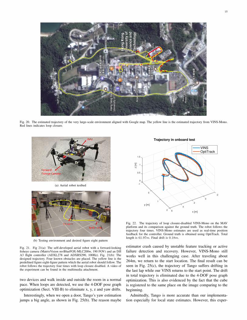
Fig. 20. The estimated trajectory of the very large-scale environment aligned with Google map. The yellow line is the estimated trajectory from VINS-Mono.Red lines indicates loop closure.

(a) Aerial robot testbed

(b) Testing environment and desired figure eight pattern

Fig. 21. Fig 21(a): The self-developed aerial robot with a forward-lookingfisheye camera (MatrixVision mvBlueFOX-MLC200w, 190 FOV) and an DJIA3 flight controller (ADXL278 and ADXRS290, 100Hz). Fig. 21(b): Thedesigned trajectory. Four known obstacles are placed. The yellow line is thepredefined figure eight-figure pattern which the aerial robot should follow. Therobot follows the trajectory four times with loop closure disabled. A video ofthe experiment can be found in the multimedia attachment.

two devices and walk inside and outside the room in a normalpace. When loops are detected, we use the 4-DOF pose graphoptimization (Sect. VIII-B) to eliminate x, y, z and yaw drifts.

Interestingly, when we open a door, Tango’s yaw estimationjumps a big angle, as shown in Fig. 25(b). The reason maybe

-2

0

Trajectory in onboard test

x [m]

2

4

62

1

y [m]

0

1.5

0

0.5

1

-1

z [m

]

VINSOptiTrack

Fig. 22. The trajectory of loop closure-disabled VINS-Mono on the MAVplatform and its comparison against the ground truth. The robot follows thetrajectory four times. VINS-Mono estimates are used as real-time positionfeedback for the controller. Ground truth is obtained using OptiTrack. Totallength is 61.97m. Final drift is 0.18m.

estimator crash caused by unstable feature tracking or activefailure detection and recovery. However, VINS-Mono stillworks well in this challenging case. After traveling about264m, we return to the start location. The final result can beseen in Fig. 25(c), the trajectory of Tango suffers drifting inthe last lap while our VINS returns to the start point. The driftin total trajectory is eliminated due to the 4-DOF pose graphoptimization. This is also evidenced by the fact that the cubeis registered to the same place on the image comparing to thebeginning.

Admittedly, Tango is more accurate than our implementa-tion especially for local state estimates. However, this exper-

16

time [s]0 20 40 60 80

x [m

]

-2

0

2

4

6

time [s]0 20 40 60 80

y [m

]

-1

0

1

2

time [s]0 20 40 60 80

z [m

]

0

0.5

1

1.5VINSOptiTrack

time [s]0 20 40 60 80

x er

ror [

m]

-0.2

0

0.2

time [s]0 20 40 60 80

y er

ror [

m]

-0.2

0

0.2

time [s]0 20 40 60 80

z er

ror [

m]

-0.2

0

0.2

time [s]0 20 40 60 80

yaw

[°]

-10

0

10

time [s]0 20 40 60 80

pitc

h [°]

-10

0

10

time [s]0 20 40 60 80

roll

[°]

-10

0

10

time [s]0 20 40 60 80

yaw

erro

r [°]

-4

-2

0

2

4

time [s]0 20 40 60 80

pitc

h er

ror [

°]

-4

-2

0

2

4

time [s]0 20 40 60 80

roll

erro

r [°]

-4

-2

0

2

4

Fig. 23. Position, orientation and their corresponding errors of loop closure-disabled VINS-Mono compared with OptiTrack. A sudden in pitch error at the60s is caused by aggressive breaking at the end of the designed trajectory, and possible time misalignment error between VINS-Mono and OptiTrack.

Fig. 24. A simple holder that we used to mount the Google Tango device(left) and the iPhone7 Plus (right) that runs our VINS-Mobile implementation.

iment shows that the proposed method can run on generalmobile devices and have the potential ability to compare spe-cially engineered devices. The robustness of proposed methodis also proved in this experiment. Video can be found in themultimedia attachment.

X. CONCLUSION AND FUTURE WORK

In this paper, we propose a robust and versatile monocularvisual-inertial estimator. Our approach features both state-of-the-art and novel solutions to IMU pre-integration, estimatorinitialization and failure recovery, online extrinsic calibration,tightly-coupled visual-inertial odometry, relocalization, andefficient global optimization. We show superior performanceby comparing against both state-of-the-art open source imple-mentations and highly optimized industry solutions. We opensource both PC and iOS implementation for the benefit of thecommunity.

Although feature-based VINS estimators have alreadyreached the maturity of real-world deployment, we still seemany directions for future research. Monocular VINS may

(a) Beginning

(b) Door opening

(c) End

Fig. 25. From left to right: AR image from VINS-Mobile, estimated trajectoryfrom VINS-Mono, estimated trajectory from Tango Fig: 25(a): Both VINS-Mobile and Tango are initialized at the start location and a virtual box isinserted on the plane which extracted from estimated features. Fig. 25(b):A challenging case in which the camera is facing a moving door. The driftof Tango trajectory is highlighted. Fig. 25(c): The final trajectory of bothVINS-Mobile and Tango. The total length is about 264m.

reach weakly observable or even degenerate conditions de-pending on the motion and the environment. We are most inter-ested in online methods to evaluate the observability propertiesof monocular VINS, and online generation of motion plans torestore observability. Another research direction concerns the

17

mass deployment of monocular VINS on a large variety ofconsumer devices, such as mobile phones. This applicationrequires online calibration of almost all sensor intrinsic andextrinsic parameters, as well as the online identification ofcalibration qualities. Finally, we are interested in producingdense maps given results from monocular VINS. Our firstresults on monocular visual-inertial dense mapping with ap-plication to drone navigation was presented in [44]. However,extensive research is still necessary to further improve thesystem accuracy and robustness.

REFERENCES

[1] G. Klein and D. Murray, “Parallel tracking and mapping for small arworkspaces,” in Mixed and Augmented Reality, 2007. ISMAR 2007. 6thIEEE and ACM International Symposium on. IEEE, 2007, pp. 225–234.

[2] C. Forster, M. Pizzoli, and D. Scaramuzza, “SVO: Fast semi-directmonocular visual odometry,” in Proc. of the IEEE Int. Conf. on Robot.and Autom., Hong Kong, China, May 2014.

[3] J. Engel, T. Schops, and D. Cremers, “Lsd-slam: Large-scale di-rect monocular slam,” in European Conference on Computer Vision.Springer International Publishing, 2014, pp. 834–849.

[4] R. Mur-Artal, J. Montiel, and J. D. Tardos, “Orb-slam: a versatileand accurate monocular slam system,” IEEE Transactions on Robotics,vol. 31, no. 5, pp. 1147–1163, 2015.

[5] J. Engel, V. Koltun, and D. Cremers, “Direct sparse odometry,” IEEETransactions on Pattern Analysis and Machine Intelligence, 2017.

[6] D. Galvez-Lopez and J. D. Tardos, “Bags of binary words for fastplace recognition in image sequences,” IEEE Transactions on Robotics,vol. 28, no. 5, pp. 1188–1197, October 2012.

[7] S. Shen, N. Michael, and V. Kumar, “Tightly-coupled monocular visual-inertial fusion for autonomous flight of rotorcraft MAVs,” in Proc. ofthe IEEE Int. Conf. on Robot. and Autom., Seattle, WA, May 2015.

[8] Z. Yang and S. Shen, “Monocular visual–inertial state estimation withonline initialization and camera–imu extrinsic calibration,” IEEE Trans-actions on Automation Science and Engineering, vol. 14, no. 1, pp.39–51, 2017.

[9] T. Qin and S. Shen, “Robust initialization of monocular visual-inertialestimation on aerial robots.” in Proc. of the IEEE/RSJ Int. Conf. onIntell. Robots and Syst., Vancouver, Canada, 2017, accepted.

[10] P. Li, T. Qin, B. Hu, F. Zhu, and S. Shen, “Monocular visual-inertialstate estimation for mobile augmented reality.” in Proc. of the IEEE Int.Sym. on Mixed adn Augmented Reality, Nantes, France, 2017, accepted.

[11] S. Weiss, M. W. Achtelik, S. Lynen, M. Chli, and R. Siegwart, “Real-time onboard visual-inertial state estimation and self-calibration of mavsin unknown environments,” in Robotics and Automation (ICRA), 2012IEEE International Conference on. IEEE, 2012, pp. 957–964.

[12] S. Lynen, M. W. Achtelik, S. Weiss, M. Chli, and R. Siegwart, “A robustand modular multi-sensor fusion approach applied to mav navigation,”in Proc. of the IEEE/RSJ Int. Conf. on Intell. Robots and Syst. IEEE,2013, pp. 3923–3929.

[13] A. I. Mourikis and S. I. Roumeliotis, “A multi-state constraint Kalmanfilter for vision-aided inertial navigation,” in Proc. of the IEEE Int. Conf.on Robot. and Autom., Roma, Italy, Apr. 2007, pp. 3565–3572.

[14] M. Li and A. Mourikis, “High-precision, consistent EKF-based visual-inertial odometry,” Int. J. Robot. Research, vol. 32, no. 6, pp. 690–711,May 2013.

[15] M. Bloesch, S. Omari, M. Hutter, and R. Siegwart, “Robust visualinertial odometry using a direct ekf-based approach,” in Proc. of theIEEE/RSJ Int. Conf. on Intell. Robots and Syst. IEEE, 2015, pp. 298–304.

[16] S. Leutenegger, S. Lynen, M. Bosse, R. Siegwart, and P. Furgale,“Keyframe-based visual-inertial odometry using nonlinear optimization,”Int. J. Robot. Research, vol. 34, no. 3, pp. 314–334, Mar. 2014.

[17] R. Mur-Artal and J. D. Tardos, “Visual-inertial monocular SLAM withmap reuse,” arXiv preprint arXiv:1610.05949, 2016.

[18] K. Wu, A. Ahmed, G. A. Georgiou, and S. I. Roumeliotis, “A squareroot inverse filter for efficient vision-aided inertial navigation on mobiledevices.” in Robotics: Science and Systems, 2015.

[19] M. K. Paul, K. Wu, J. A. Hesch, E. D. Nerurkar, and S. I. Roumeliotis,“A comparative analysis of tightly-coupled monocular, binocular, andstereo vins,” in Proc. of the IEEE Int. Conf. on Robot. and Autom.,Singapore, May 2017.

[20] M. Kaess, H. Johannsson, R. Roberts, V. Ila, J. J. Leonard, andF. Dellaert, “isam2: Incremental smoothing and mapping using the bayestree,” The International Journal of Robotics Research, vol. 31, no. 2, pp.216–235, 2012.

[21] V. Usenko, J. Engel, J. Stuckler, and D. Cremers, “Direct visual-inertialodometry with stereo cameras,” in Proc. of the IEEE Int. Conf. on Robot.and Autom. IEEE, 2016, pp. 1885–1892.

[22] T. Lupton and S. Sukkarieh, “Visual-inertial-aided navigation for high-dynamic motion in built environments without initial conditions,” IEEETrans. Robot., vol. 28, no. 1, pp. 61–76, Feb. 2012.

[23] C. Forster, L. Carlone, F. Dellaert, and D. Scaramuzza, “IMU prein-tegration on manifold for efficient visual-inertial maximum-a-posterioriestimation,” in Proc. of Robot.: Sci. and Syst., Rome, Italy, Jul. 2015.

[24] S. Shen, Y. Mulgaonkar, N. Michael, and V. Kumar, “Initialization-free monocular visual-inertial estimation with application to autonomousMAVs,” in Proc. of the Int. Sym. on Exp. Robot., Marrakech, Morocco,Jun. 2014.

[25] A. Martinelli, “Closed-form solution of visual-inertial structure frommotion,” Int. J. Comput. Vis., vol. 106, no. 2, pp. 138–152, 2014.

[26] J. Kaiser, A. Martinelli, F. Fontana, and D. Scaramuzza, “Simultaneousstate initialization and gyroscope bias calibration in visual inertial aidednavigation,” IEEE Robotics and Automation Letters, vol. 2, no. 1, pp.18–25, 2017.

[27] M. Faessler, F. Fontana, C. Forster, and D. Scaramuzza, “Automatic re-initialization and failure recovery for aggressive flight with a monocularvision-based quadrotor,” in Proc. of the IEEE Int. Conf. on Robot. andAutom. IEEE, 2015, pp. 1722–1729.

[28] H. Strasdat, J. Montiel, and A. J. Davison, “Scale drift-aware large scalemonocular slam,” Robotics: Science and Systems VI, 2010.

[29] B. D. Lucas and T. Kanade, “An iterative image registration techniquewith an application to stereo vision,” in Proc. of the Intl. Joint Conf. onArtificial Intelligence, Vancouver, Canada, Aug. 1981, pp. 24–28.

[30] J. Shi and C. Tomasi, “Good features to track,” in Computer Visionand Pattern Recognition, 1994. Proceedings CVPR’94., 1994 IEEEComputer Society Conference on. IEEE, 1994, pp. 593–600.

[31] R. Hartley and A. Zisserman, Multiple view geometry in computer vision.Cambridge university press, 2003.

[32] A. Heyden and M. Pollefeys, “Multiple view geometry,” EmergingTopics in Computer Vision, 2005.

[33] D. Nister, “An efficient solution to the five-point relative pose problem,”IEEE transactions on pattern analysis and machine intelligence, vol. 26,no. 6, pp. 756–770, 2004.

[34] T. Liu and S. Shen, “Spline-based initialization of monocular visual-inertial state estimators at high altitude,” IEEE Robotics and AutomationLetters, 2017, accepted.

[35] V. Lepetit, F. Moreno-Noguer, and P. Fua, “Epnp: An accurate o (n)solution to the pnp problem,” International journal of computer vision,vol. 81, no. 2, pp. 155–166, 2009.

[36] B. Triggs, P. F. McLauchlan, R. I. Hartley, and A. W. Fitzgibbon,“Bundle adjustmenta modern synthesis,” in International workshop onvision algorithms. Springer, 1999, pp. 298–372.

[37] P. Huber, “Robust estimation of a location parameter,” Annals ofMathematical Statistics, vol. 35, no. 2, pp. 73–101, 1964.

[38] S. Agarwal, K. Mierle, and Others, “Ceres solver,” http://ceres-solver.org.

[39] G. Sibley, L. Matthies, and G. Sukhatme, “Sliding window filter withapplication to planetary landing,” J. Field Robot., vol. 27, no. 5, pp.587–608, Sep. 2010.

[40] M. Calonder, V. Lepetit, C. Strecha, and P. Fua, “Brief: Binary robustindependent elementary features,” Computer Vision–ECCV 2010, pp.778–792, 2010.

[41] M. Burri, J. Nikolic, P. Gohl, T. Schneider, J. Rehder, S. Omari, M. W.Achtelik, and R. Siegwart, “The euroc micro aerial vehicle datasets,”The International Journal of Robotics Research, 2016.

[42] C. Mei and P. Rives, “Single view point omnidirectional camera cal-ibration from planar grids,” in Robotics and Automation, 2007 IEEEInternational Conference on. IEEE, 2007, pp. 3945–3950.

[43] L. Heng, B. Li, and M. Pollefeys, “Camodocal: Automatic intrinsicand extrinsic calibration of a rig with multiple generic cameras andodometry,” in Intelligent Robots and Systems (IROS), 2013 IEEE/RSJInternational Conference on. IEEE, 2013, pp. 1793–1800.

[44] Y. Lin, F. Gao, T. Qin, W. Gao, T. Liu, W. Wu, Z. Yang, and S. Shen,“Autonomous aerial navigation using monocular visual-inertial fusion,”J. Field Robot., vol. 00, pp. 1–29, 2017.