Embed Size (px)
Citation preview
Viking GCMS Data Restoral and Perceiving Temperature on Other
Worlds: Astrobiology Projects at NASA Ames
Melissa Guzman
Internship Report submitted to the International Space University in partial fulfillment of the
requirements of the M.Sc. Degree in Space Studies
August, 2015
Internship Mentor: Dr. Christopher McKay
Host Institution: NASA Ames Research Center, Mountain View, CA, USA
ISU Academic Advisor: Dr. Hugh Hill
i
Abstract The primary task for the summer was to procure the GCMS data from the National Space Science
Data Coordinated Archive (NSSDCA) and to assess the current state of the data set for possible
reanalysis opportunities. After procurement of the Viking GCMS data set and analysis of its
current state, the internship focus shifted to preparing a plan for restoral and archiving of the
GCMS data set. A proposal was prepared and submitted to NASA Headquarters to restore and
make available the 8000 mass chromatographs that are the basic data generated by the Viking
GCMS instrument. The relevance of this restoral and the methodology we propose for restoral is
presented.
The secondary task for the summer is to develop a thermal model for the perceived temperature
of a human standing on Mars, Titan, or Europa. Traditionally, an equation called “Fanger’s
comfort equation” is used to measure the perceived temperature by a human in a given
reference environment. However, there are limitations to this model when applied to other
planets. Therefore, the approach for this project has been to derive energy balance equations
from first principles and then develop a methodology for correlating “comfort” to energy
balance. Using the -20°C walk-in freezer in the Space Sciences building at NASA Ames, energy loss
of a human subject is measured. Energy loss for a human being on Mars, Titan and Europa are
calculated from first principles. These calculations are compared to the freezer measurements,
e.g. for 1 minute on Titan, a human loses as much energy as x minutes in a -20°C freezer. This
gives a numerical comparison between the environments. These energy calculations are used to
consider the physiological comfort of a human based on the calculated energy losses.
Acknowledgements Thank you to my internship advisor, Chris McKay, for his clear and infectious scientific curiosity,
his constant supply of original project ideas, and his generosity of time and mentorship.
Thank you to my ISU advisor, Hugh Hill, for his unrelenting encouragement and his helpful
foresight.
Thank you also to my comrades in the cubicles, James Bevington, Patrick Carlson, and Jade
Checlair, who were always there to bounce ideas around.
ii
Contents
Abstract ............................................................................................................................................ i
Acknowledgements .......................................................................................................................... i
Table of Tables ................................................................................................................................ iii
Table of Figures ............................................................................................................................... iii
Abbreviations .................................................................................................................................. iv
1. Introduction ............................................................................................................................. 1
2. Restoral and archiving of Viking GCMS data sets ....................................................................... 3
2.1 Viking Restoral Objectives ..................................................................................................... 3
2.2 Viking GCMS Background Work and Motivations ................................................................. 4
2.3 Applications of Restored Viking Data .................................................................................... 7
2.4 Current state of the Viking GCMS datasets ......................................................................... 12
2.5 Proposed plan for Viking GCMS data restoration ............................................................... 14
2.6 Submission of PDART proposal and future plans ................................................................ 21
3. Modelling perceived temperature of the human body on other planets ............................. 22
3.1 Perceived Temperature Objectives ..................................................................................... 22
3.2 Perceived Temperature Background Work and Motivations ............................................. 22
3.3 Mojave Desert field measurements .................................................................................... 25
3.4 Plan of action for perceived temperature future progress ................................................. 27
4. Internship Benefits to the Student ........................................................................................ 31
5. Conclusion ............................................................................................................................. 32
References .................................................................................................................................... 35
Appendix ....................................................................................................................................... 37
iii
Table of Tables Table 1: Objectives for the Viking restoral project. ........................................................................ 4
Table 2: Comparison of elution times. .......................................................................................... 11
Table 3: Current known information on the digital Viking GCMS data. ....................................... 14
Table 4: Summary of plan for data restoral. ................................................................................. 15
Table 5: Examples of clues from Biemann et al. 1977 of possible use for restoring data set. ..... 17
Table 6: Solution utilized to open, split and export Viking data set. ............................................ 19
Table 7: Objectives for the perceived temperature project. ........................................................ 22
Table 8: Measurements for perceived temperature calculations taken at Silver Lake. ............... 25
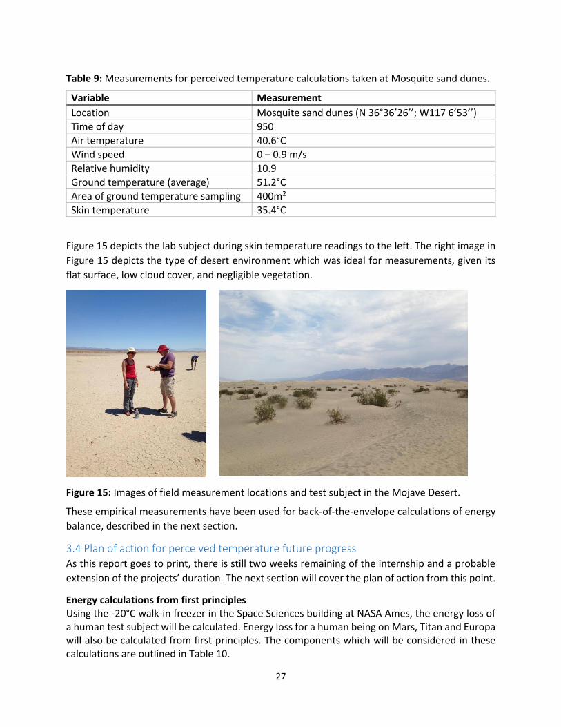
Table 9: Measurements for perceived temperature calculations taken at Mosquite. ................ 27
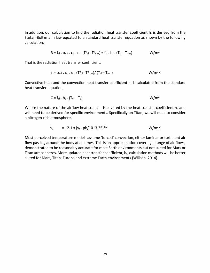
Table 10: Main energy considerations for energy calculations from first principles. .................. 28
Table 11: Proposed methods for correlating energy balance with comfort level ........................ 30
Table 13: Recommendations for continuation of projects. .......................................................... 34
Table 14: Full document of clues from Biemann et al. 1977. ....................................................... 37
Table 15: Table of variables for Perceived Temperature ............................................................. 39
Table of Figures Figure 1: A screen shot from the short film, Wanderers. ............................................................... 2
Figure 2: An illustration of how to read this report by chapter and sections ................................ 3
Figure 3: A full depiction of Mars exploration by crafts sent from Earth.. ..................................... 5
Figure 4: An example of helpful cataloguing of the GCMS data. .................................................... 8
Figure 5: Chlorobenzene detection by SAM on Mars.. ................................................................. 11
Figure 6: Mass chromatographs of m/e 128 ................................................................................ 12
Figure 7: The mass chromatogram of m/e 50 from the 200°C experiment. ................................ 16
Figure 8: A screenshot of the Viking GCMS data .......................................................................... 18
Figure 9: Working solution for cataloging GCMS data set. ........................................................... 19
Figure 10: Example of GCMS data set indexing so far in preparation for restoration ................. 20
Figure 11: Plot of first 1,000 data points from one file of VL-1 GCMS data. ................................ 20
Figure 12: Modes of heat transfer between the human body and an environment. .................. 23
Figure 13: Energy balance equation for the human body. ........................................................... 23
Figure 14: Flow diagram of Perceived Temperature applying PMV metod ................................. 26
Figure 15: Images of field measurement locations and test subject in the Mojave Desert. ........ 27
Figure 16: Examples of simple and detailed geometry in full body human thermal modelling. . 31
iv
Abbreviations
GC Gas Chromatograph
GCMS Gas Chromatography Mass Spectrometry
GEX Gas Exchange (Instrument)
ITAR International Traffic in Arms Regulations
LR Labelled Release (Instrument)
MS Mass Spectrometer
NASA National Aeronautics and Space Administration
NIST National Institute of Standards and Technology
NSSDCA National Space Science Data Coordinated Archive
PMV Predicted Mean Vote
PR Pyrolytic Release (Instrument)
PT Perceived Temperature
SAM Sample Analysis on Mars
TEGA Thermal Evolved Gas Analysis
VL Viking Lander
VL-1 Viking Lander 1
VL-2 Viking Lander 2
1
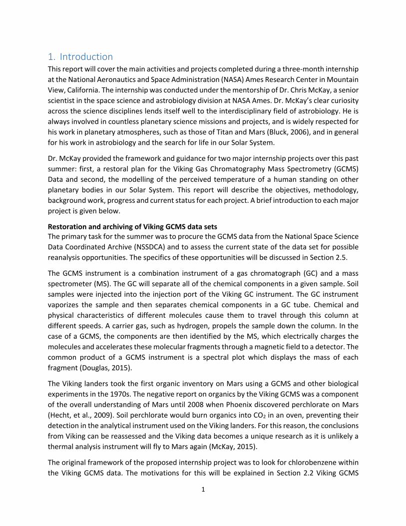
1. Introduction This report will cover the main activities and projects completed during a three-month internship
at the National Aeronautics and Space Administration (NASA) Ames Research Center in Mountain
View, California. The internship was conducted under the mentorship of Dr. Chris McKay, a senior
scientist in the space science and astrobiology division at NASA Ames. Dr. McKay’s clear curiosity
across the science disciplines lends itself well to the interdisciplinary field of astrobiology. He is
always involved in countless planetary science missions and projects, and is widely respected for
his work in planetary atmospheres, such as those of Titan and Mars (Bluck, 2006), and in general
for his work in astrobiology and the search for life in our Solar System.
Dr. McKay provided the framework and guidance for two major internship projects over this past
summer: first, a restoral plan for the Viking Gas Chromatography Mass Spectrometry (GCMS)
Data and second, the modelling of the perceived temperature of a human standing on other
planetary bodies in our Solar System. This report will describe the objectives, methodology,
background work, progress and current status for each project. A brief introduction to each major
project is given below.
Restoration and archiving of Viking GCMS data sets The primary task for the summer was to procure the GCMS data from the National Space Science
Data Coordinated Archive (NSSDCA) and to assess the current state of the data set for possible
reanalysis opportunities. The specifics of these opportunities will be discussed in Section 2.5.
The GCMS instrument is a combination instrument of a gas chromatograph (GC) and a mass
spectrometer (MS). The GC will separate all of the chemical components in a given sample. Soil
samples were injected into the injection port of the Viking GC instrument. The GC instrument
vaporizes the sample and then separates chemical components in a GC tube. Chemical and
physical characteristics of different molecules cause them to travel through this column at
different speeds. A carrier gas, such as hydrogen, propels the sample down the column. In the
case of a GCMS, the components are then identified by the MS, which electrically charges the
molecules and accelerates these molecular fragments through a magnetic field to a detector. The
common product of a GCMS instrument is a spectral plot which displays the mass of each
fragment (Douglas, 2015).
The Viking landers took the first organic inventory on Mars using a GCMS and other biological
experiments in the 1970s. The negative report on organics by the Viking GCMS was a component
of the overall understanding of Mars until 2008 when Phoenix discovered perchlorate on Mars
(Hecht, et al., 2009). Soil perchlorate would burn organics into CO2 in an oven, preventing their
detection in the analytical instrument used on the Viking landers. For this reason, the conclusions
from Viking can be reassessed and the Viking data becomes a unique research as it is unlikely a
thermal analysis instrument will fly to Mars again (McKay, 2015).
The original framework of the proposed internship project was to look for chlorobenzene within
the Viking GCMS data. The motivations for this will be explained in Section 2.2 Viking GCMS
2
Background Work and Motivations. After procurement of the Viking GCMS data set and analysis
of its current state, the internship focus shifted to preparing a plan for restoral and archiving of
the GCMS data set. A proposal was prepared and submitted to NASA Headquarters to restore
and make available the 8000 mass chromatographs that are the basic data generated by the
Viking GCMS instrument. The relevance of this restoral and the methodology we propose for
restoral will be presented in Section 2.5.
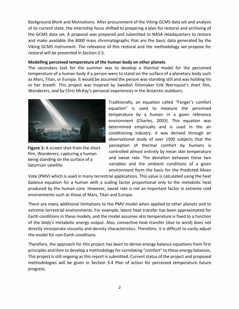
Modelling perceived temperature of the human body on other planets The secondary task for the summer was to develop a thermal model for the perceived temperature of a human body if a person were to stand on the surface of a planetary body such as Mars, Titan, or Europa. It would be assumed the person was standing still and was holding his or her breath. This project was inspired by Swedish filmmaker Erik Wernquist’s short film, Wanderers, and by Chris McKay’s personal experiences in the Antarctic outdoors.
Traditionally, an equation called “Fanger’s comfort
equation” is used to measure the perceived
temperature by a human in a given reference
environment (Charles, 2003). This equation was
determined empirically and is used in the air
conditioning industry. It was derived through an
observational study of over 1500 subjects that the
perception of thermal comfort by humans is
controlled almost entirely by mean skin temperature
and sweat rate. The deviation between these two
variables and the ambient conditions of a given
environment form the basis for the Predicted Mean
Vote (PMV) which is used in many terrestrial applications. This value is calculated using the heat
balance equation for a human with a scaling factor proportional only to the metabolic heat
produced by the human core. However, sweat rate is not an important factor in extreme cold
environments such as those of Mars, Titan and Europa.
There are many additional limitations to the PMV model when applied to other planets and to
extreme terrestrial environments. For example, latent heat transfer has been approximated for
Earth conditions in these models, and the model assumes skin temperature is fixed to a function
of the body’s metabolic energy output. Also, convective heat transfer (due to wind) does not
directly incorporate viscosity and density characteristics. Therefore, it is difficult to easily adjust
the model for non-Earth conditions.
Therefore, the approach for this project has been to derive energy balance equations from first
principles and then to develop a methodology for correlating “comfort” to these energy balances.
This project is still ongoing as this report is submitted. Current status of the project and proposed
methodologies will be given in Section 3.4 Plan of action for perceived temperature future
progress.
Figure 1: A screen shot from the short film, Wanderers, capturing a human being standing on the surface of a Saturnian satellite.
3
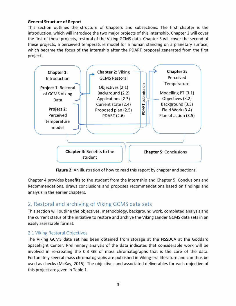
General Structure of Report This section outlines the structure of Chapters and subsections. The first chapter is the introduction, which will introduce the two major projects of this internship. Chapter 2 will cover the first of these projects, restoral of the Viking GCMS data. Chapter 3 will cover the second of these projects, a perceived temperature model for a human standing on a planetary surface, which became the focus of the internship after the PDART proposal generated from the first project.
Chapter 4 provides benefits to the student from the internship and Chapter 5, Conclusions and
Recommendations, draws conclusions and proposes recommendations based on findings and
analysis in the earlier chapters.
2. Restoral and archiving of Viking GCMS data sets This section will outline the objectives, methodology, background work, completed analysis and
the current status of the initiative to restore and archive the Viking Lander GCMS data sets in an
easily assessable format.
2.1 Viking Restoral Objectives The Viking GCMS data set has been obtained from storage at the NSSDCA at the Goddard
Spaceflight Center. Preliminary analysis of the data indicates that considerable work will be
involved in re-creating the 0.3 GB of mass chromatographs that is the core of the data.
Fortunately several mass chromatographs are published in Viking-era literature and can thus be
used as checks (McKay, 2015). The objectives and associated deliverables for each objective of
this project are given in Table 1.
Chapter 4: Benefits to the student
Chapter 1:
Introduction
Project 1: Restoral
of GCMS Viking
Data
Project 2:
Perceived
temperature
model
Chapter 5: Conclusions
Chapter 2: Viking
GCMS Restoral
Objectives (2.1) Background (2.2) Applications (2.3) Current state (2.4)
Proposed plan (2.5) PDART (2.6)
Chapter 3:
Perceived
Temperature
Modelling PT (3.1) Objectives (3.2)
Background (3.3) Field Work (3.4)
Plan of action (3.5)
Figure 2: An illustration of how to read this report by chapter and sections.
PD
AR
T su
bm
issi
on
4
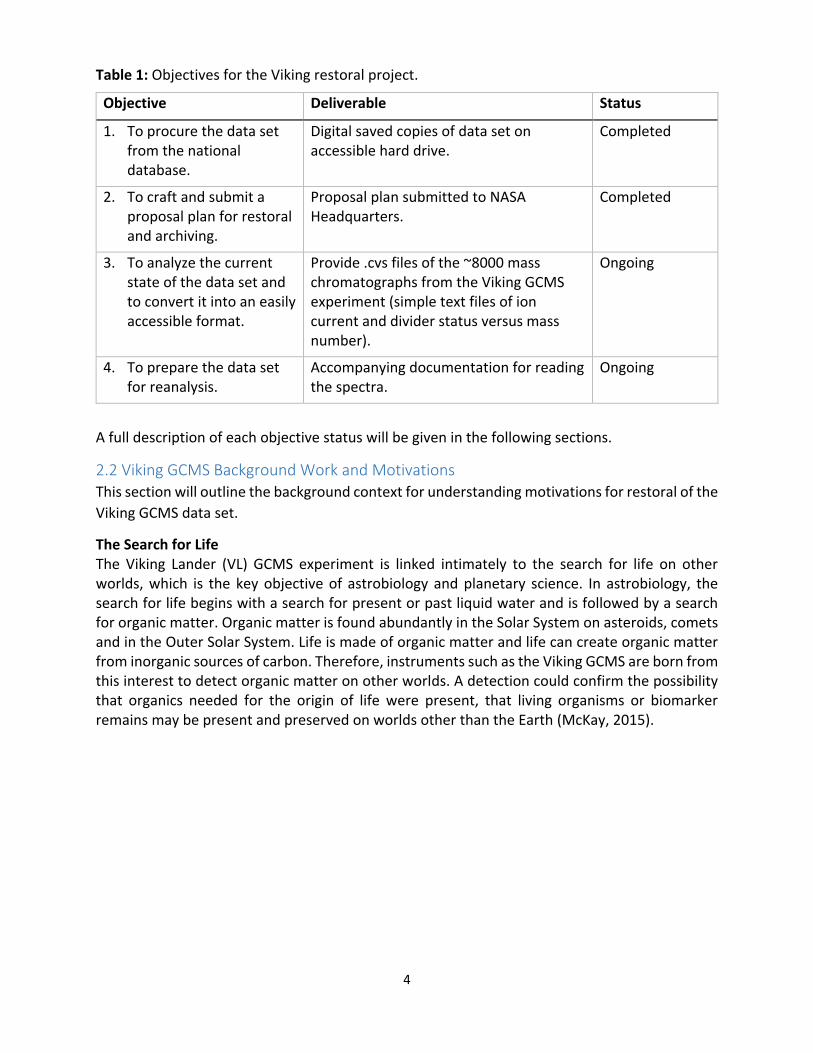
Table 1: Objectives for the Viking restoral project.
Objective Deliverable Status
1. To procure the data set from the national database.
Digital saved copies of data set on accessible hard drive.
Completed
2. To craft and submit a proposal plan for restoral and archiving.
Proposal plan submitted to NASA Headquarters.
Completed
3. To analyze the current state of the data set and to convert it into an easily accessible format.
Provide .cvs files of the ~8000 mass chromatographs from the Viking GCMS experiment (simple text files of ion current and divider status versus mass number).
Ongoing
4. To prepare the data set for reanalysis.
Accompanying documentation for reading the spectra.
Ongoing
A full description of each objective status will be given in the following sections.
2.2 Viking GCMS Background Work and Motivations This section will outline the background context for understanding motivations for restoral of the
Viking GCMS data set.
The Search for Life The Viking Lander (VL) GCMS experiment is linked intimately to the search for life on other worlds, which is the key objective of astrobiology and planetary science. In astrobiology, the search for life begins with a search for present or past liquid water and is followed by a search for organic matter. Organic matter is found abundantly in the Solar System on asteroids, comets and in the Outer Solar System. Life is made of organic matter and life can create organic matter from inorganic sources of carbon. Therefore, instruments such as the Viking GCMS are born from this interest to detect organic matter on other worlds. A detection could confirm the possibility that organics needed for the origin of life were present, that living organisms or biomarker remains may be present and preserved on worlds other than the Earth (McKay, 2015).
5
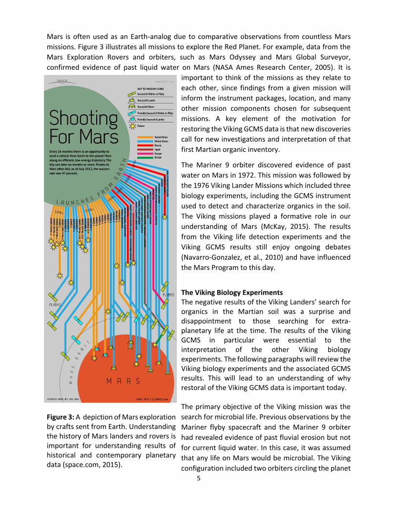
Mars is often used as an Earth-analog due to comparative observations from countless Mars
missions. Figure 3 illustrates all missions to explore the Red Planet. For example, data from the
Mars Exploration Rovers and orbiters, such as Mars Odyssey and Mars Global Surveyor,
confirmed evidence of past liquid water on Mars (NASA Ames Research Center, 2005). It is
important to think of the missions as they relate to
each other, since findings from a given mission will
inform the instrument packages, location, and many
other mission components chosen for subsequent
missions. A key element of the motivation for
restoring the Viking GCMS data is that new discoveries
call for new investigations and interpretation of that
first Martian organic inventory.
The Mariner 9 orbiter discovered evidence of past
water on Mars in 1972. This mission was followed by
the 1976 Viking Lander Missions which included three
biology experiments, including the GCMS instrument
used to detect and characterize organics in the soil.
The Viking missions played a formative role in our
understanding of Mars (McKay, 2015). The results
from the Viking life detection experiments and the
Viking GCMS results still enjoy ongoing debates
(Navarro-Gonzalez, et al., 2010) and have influenced
the Mars Program to this day.
The Viking Biology Experiments The negative results of the Viking Landers’ search for organics in the Martian soil was a surprise and disappointment to those searching for extra-planetary life at the time. The results of the Viking GCMS in particular were essential to the interpretation of the other Viking biology experiments. The following paragraphs will review the Viking biology experiments and the associated GCMS results. This will lead to an understanding of why restoral of the Viking GCMS data is important today. The primary objective of the Viking mission was the
search for microbial life. Previous observations by the
Mariner flyby spacecraft and the Mariner 9 orbiter
had revealed evidence of past fluvial erosion but not
for current liquid water. In this case, it was assumed
that any life on Mars would be microbial. The Viking
configuration included two orbiters circling the planet
Figure 3: A depiction of Mars exploration by crafts sent from Earth. Understanding the history of Mars landers and rovers is important for understanding results of historical and contemporary planetary data (space.com, 2015).
6
repeatedly photographing and monitoring its surface along with two landers, Viking Lander 1 (VL-
1) and Viking Lander 2 (VL-2), which touched down at Chryse Planitia and Utopia Planitia
respectively (NASA Mars Exploration, 2015).
In addition to the GCMS instrument, there were three biology instruments on each lander: the
pyrolytic release (PR) instrument, the labeled release (LR) instrument, and the gas exchange
(GEX) instrument all incubated samples of the Martian soil under different environmental
conditions (NSSDC, 2014). The following paragraphs will outline those instruments, their results,
and interpretations of these results.
The PR experiment (Horowitz, et al., 1976) searched for evidence of photosynthesis as a sign of
life. It was believed that photosynthetic organisms would convert carbon to biomass through
carbon fixation which could be detected by a radioactivity counter after vaporization. The first
run of the experiment had a significant response from the counter. Although well below the
typical response observed in terrestrial biotic samples, the response was still much over the noise
level. However, subsequent trials did not reproduce the high result. At the end the initial
response was attributed to a prelaunch contamination.
The GEX experiment (Oyama & Berdahl, 1977) searched for heterotrophs, microorganisms
capable of consuming organic material. The GEX was designed to detect gases released as a by-
product of the microbial metabolism, i.e. bacterial flatulence (McKay, 2015). A soil sample was
placed in the instrument chamber and equilibrated with water vapor before being combined with
a nutrient solution. Samples of the gas were then removed and analyzed by the gas
chromatograph. The GEX detected released oxygen gas levels of 70 to 700 nanomoles per gram
of soil. This level of oxygen release could not be attributed to ambient atmospheric oxygen
absorbed onto the soil grains, but rather had to be attributed to a chemical or biological reaction.
Unfortunately, it was concluded that a biological explanation was unlikely since the levels of
oxygen release persisted over temperatures of 160°C. In addition, adding the nutrient solution
did not change the result, indicating that some chemical in the soil must be highly reactive with
water.
The third biology experiment, the LR experiment (Levin & Straat, 1977), also searched for
evidence of heterotrophic organisms. In this experiment, a solution of water with seven organic
compounds was added to the soil. The carbon atoms were radioactive in each compound. Any
carbon metabolism in the soil would be detected by a radiation detector as organisms consumed
the organics and released radioactive CO2 (McKay, 2015). A steady release of reactive CO2 was
detected during the experiment runs. These results, if taken alone, would have had the strongest
positive indication for the presence of Martian microbial life.
The GCMS Instrument Although the results of the LR experiment might have been interpreted in favor of life on Mars, there was also the Viking GCMS data which had to be considered in parallel. The GCMS instrument and its data set is the focus of this internship project. The reasons for this are elaborated in the following paragraphs.
7
The GCMS instrument received Martian soil samples from the same sampling arm that provided
soil to the biology experiments. Each soil sample was heated to 500°C which would release any
organics. These organics were carried through the gas chromatograph column and were then
identified by the mass spectrometer as described in the Introduction. The results from this
experiment were that no organics were detected. This was and still is a hugely surprising result.
The GCMS could detect a concentration of organics on the order of one part per billion with one
part per billion in a soil sample representing over a million individual bacterium. This result then
does not even correlate with contemporary known meteoritic influx of organics on Mars (McKay,
2015).
This apparent absence of organic material detected by the GCMS then was the main argument
against a biological interpretation of the positive LR results (Klein 1999). This negative detection
for organics became part of the overall understanding of Mars until 2008 when Phoenix
discovered perchlorate on Mars (Hecht, et al., 2009).
Perchlorate on Mars and reassessment of Viking GCMS results Dichloromethane and chloromethane were detected by the Viking Landers but were dismissed
as terrestrial contaminants, even though they were not detected in the blank runs. However, the
finding by the Phoenix mission to Mars that the dominant form of chlorine on Mars is as
perchlorate (Hecht, et al., 2009) has provided the key to understanding the Viking results
(Navarro-Gonzalez, et al., 2010). The heating of perchlorate would have caused a decomposition
into reactive O and Cl, oxidizing any organics and producing the dichloromethane and
chloromethane which was detected. This has been confirmed by results from the Curiosity Rover
at the Martian equator (Freissinet, et al., 2015). In addition, ionizing radiation would decompose
perchlorate in the Martian soil and that would result in the formation of hypochlorite, other
lower oxidation state oxychlorine species, with a concomitant production of O2 gas that remains
trapped in the salt crystal (Quinn et al. 2013). The presence of hypochlorite provides an
explanation for the LR results and the trapped O2 gas provides an explanation for the GEX results.
These reactive forms of chlorine would have broken down any naturally occurring organic
material or any material carried to the Martian surface by meteorites (McKay, 2015).
2.3 Applications of Restored Viking Data This section will explain possible opportunities for further analysis or reanalysis which would be
available if the Viking data were to be restored. The importance of the Viking data restoral will
be presented using concrete case studies.
Understanding the Viking GCMS data from the literature This section will outline the Viking GCMS data set as understood from the literature and will briefly describe the parameters of the GCMS instrument. A basic understanding of the Viking GCMS instrument is necessary for possible eventual deciphering of the data set. The fundamental data set generated by the Viking GCMS instruments are mass scans from the
mass spectrometer which reads the samples broken apart by the GC. The mass spectrometer was
reported to have a dynamic range of 6-7 orders of magnitude and a mass range (m/e) of 12-200
(Biemann, et al., 1977).
8
Mass scans were obtained directly from the Martian atmosphere and from the output of the GC
column. In the second mode, scans were made every 10.42 seconds and up to 500 scans were
produced for each run. The total data set is 16 GCMS runs (two blank runs, five runs at the first
landing site, and nine runs at the second landing site) for the analysis of four soil samples total.
This published information could possibly help restore the data, as will be explained in Section
2.5.
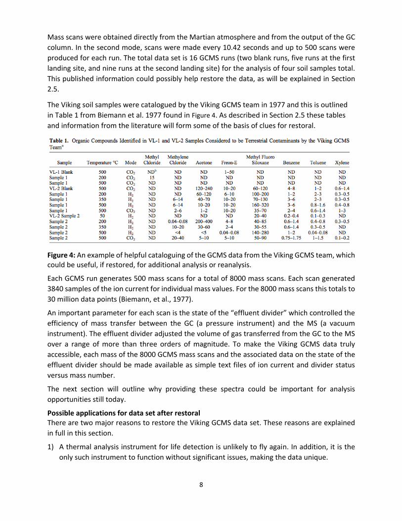
The Viking soil samples were catalogued by the Viking GCMS team in 1977 and this is outlined
in Table 1 from Biemann et al. 1977 found in Figure 4. As described in Section 2.5 these tables
and information from the literature will form some of the basis of clues for restoral.
Figure 4: An example of helpful cataloguing of the GCMS data from the Viking GCMS team, which could be useful, if restored, for additional analysis or reanalysis.
Each GCMS run generates 500 mass scans for a total of 8000 mass scans. Each scan generated
3840 samples of the ion current for individual mass values. For the 8000 mass scans this totals to
30 million data points (Biemann, et al., 1977).
An important parameter for each scan is the state of the “effluent divider” which controlled the
efficiency of mass transfer between the GC (a pressure instrument) and the MS (a vacuum
instrument). The effluent divider adjusted the volume of gas transferred from the GC to the MS
over a range of more than three orders of magnitude. To make the Viking GCMS data truly
accessible, each mass of the 8000 GCMS mass scans and the associated data on the state of the
effluent divider should be made available as simple text files of ion current and divider status
versus mass number.
The next section will outline why providing these spectra could be important for analysis
opportunities still today.
Possible applications for data set after restoral There are two major reasons to restore the Viking GCMS data set. These reasons are explained
in full in this section.
1) A thermal analysis instrument for life detection is unlikely to fly again. In addition, it is the
only such instrument to function without significant issues, making the data unique.
9
2) Reanalysis of the Viking GCMS data for scientific purposes as new information is added to the
literature.
The Viking GCMS was the first analytical chemical instrument on Mars and, to date, the only one
that has operated without significant instrument issues (McKay, 2015). The 2007 Phoenix Mission
carried a Thermal Evolved Gas Analysis (TEGA) instrument which reported the detection of CO2
released from carbonates (Boynton, et al., 2009) and O2 released from perchlorates (Hecht, et
al., 2009) but no analysis of the TEGA data has been published with respect to detection of
organics. The instrument itself had significant operational issues due to a nickel coating on the
oven walls which reacted with the perchlorate.
The Curiosity mission carried the Sample Analysis on Mars (SAM) instrument which included an
evolved gas analysis based on a head-space MS as well as a GCMS mode. SAM carried nine sealed
containers of derivatization agents, including MTBSTFA, which are used to modify some
compounds into other compounds with properties more easily analyzed in the GC process.
Unfortunately, one of the MTBSTFA containers leaked during flight and this created a large
organic background of both C and N compounds in the instrument. During analysis, the MTBSTFA
reacted with the perchlorate in the soil, creating a host of chlorinated organics derived from the
MTBSTFA contamination. After extraordinary effort and ingenuity, the SAM team confirmed
Martian organics by a detection of chlorobenzene in one sample at much higher levels than could
be explained by contamination (Freissinet, et al., 2015). It is also important to note that although
the SAM instrument arrived at Mars after the discovery of perchlorate, the SAM instrument was
designed and built before this discovery (McKay, 2015).
In light of the discovery of perchlorate on Mars (Hecht, et al., 2009), the implications for thermal
analysis (Navarro-Gonzalez, et al., 2010), and the confirmation of perchlorate at Gale Crater
(Glavin, et al., 2014), a thermal analysis instrument will not fly to Mars again. The Viking data is
unique as a thermal analysis instrument which did not suffer operational issues. This research
then should be made easily available.
The Viking GCMS team did analyze and publish on the data. However, recent cases have shown
that the Viking data needs to be available as new scientific questions arise. The following two
cases are examples of scientific questions which have come to light since the 1970s and have
been called into question within the scientific community and in which the Viking data could be
useful. One of these cases is resolved while the other is not. This second unresolved case forms
a foundational basis for the motivation of Viking GCMS restoral at this time.
Case 1: Ar/N2 ratio In addition to analyzing soil samples, the Viking GCMS also analyzed atmospheric gases on Mars. This experiment found that N2 and Ar were the second and third most abundant gases in the Martian atmosphere. The Ar/N2 ratio was determined to be 0.59 (Owen & Bar-Nun, 1995) by Viking. SAM measured the Ar/N2 ratio to be 1.02, which is about 1.7x the value determined by the Viking GCMS experiment. It was suggested that the discrepancy was due to different instrument characteristics and that SAM offered a more accurate determination of the gas ratio (Maffahy, et al., 2013).
10
A reanalysis of the Viking data was initiated, which ultimately led to the conclusion that Viking
had produced a more accurate result than the later SAM instrument. This conclusion came from
the fact that the GEX instrument offered an independent analysis of the ratio in agreement with
the GCMS (Oyama & Berdahl, 1977). In addition, analysis of Martian meteorites indicate a long
term average value of Ar/N on Mars in agreement with the Viking results. Although this case has
been resolved, it illustrates how a reanalysis of the Viking data could be required as more
discoveries in planetary exploration are made (McKay, 2015).
Case 2: The detection of chlorobenzene Although dismissed as terrestrial contamination at the time, chloromethane (CH3Cl) was detected by VL-1 and dichloromethane (CH2Cl2) was detected by VL-2. However, no CH2Cl2 was detected in blank runs of the GCMS or in sample runs at temperatures below 300°C (Biemann, et al., 1977). After perchlorate was discovered by the Phoenix lander, Navarro-Gonzalez et al. (2010) suggested that the CH3Cl and CH2Cl2 detected by VL1 and VL2, respectively, was due to the reaction of soil perchlorates and soil organics when the samples were heated above about 350°C. Sam has detected CH3Cl and CH2Cl2, but this is clearly due to the leaked MTBCSFA reacting with the soil perchlorate. However, it has been argued that chlorobenzene detected in the Cumberland sample on Mars represents a reaction product of Martian organics with Martian perchlorates (Freissinet, et al., 2015). The chlorobenzene level in this sample is 5x higher than in any other sample or blank. It has also been found in terrestrial analog studies that benzene is the dominant organic fragment released when the organic-poor soils of the hyper arid region of the Atacama desert undergo heating (Navarro-Gonzalez, et al., 2003).
For this reason, it would be interesting to search for chlorobenzene in the Viking GCMS data.
Chlorobenzene was not present in the GCMS data as a clearly defined peak or it would have been
reported by the Viking team (Biemann, et al., 1977). However, it may be that data analysis
focused on this compound and motivated by the knowledge of perchlorate in the Martian soil
would indicate chlorobenzene is present at a statistically plausible level (McKay, 2015). This
interest formed the basis for restoration plans this summer, and it has been the major motivation
behind correspondence with Klaus Biemann, the Viking GCMS Primary Investigator. This
correspondence will be further discussed in terms of methodology of restoral plans in Section
2.5.
Searching for chlorobenzene in the Viking data set Unfortunately the state of the Viking GCMS dataset was underestimated at the beginning of the summer, and while the search for chlorobenzene will hopefully come later, the majority of the focus over the summer turned toward restoration plans. This section will outline how the Viking data set could potentially be used to look for chlorobenzene. As discussed above, Freissinet et al. (2015) have reported chlorobenzene produced from heating
of a Martian sample from the Cumberland drill hole in the Sheepbed Formation at Yellowknife
Bay in Gale Crater on Mars. It could be of interest then to search the Viking GCMS data for
chlorobenzene and set an upper limit to describe its presence in the data set. The data needed
for this analysis would be the atomic mass values for chlorobenzene isotopes (the m/e=112 and
11
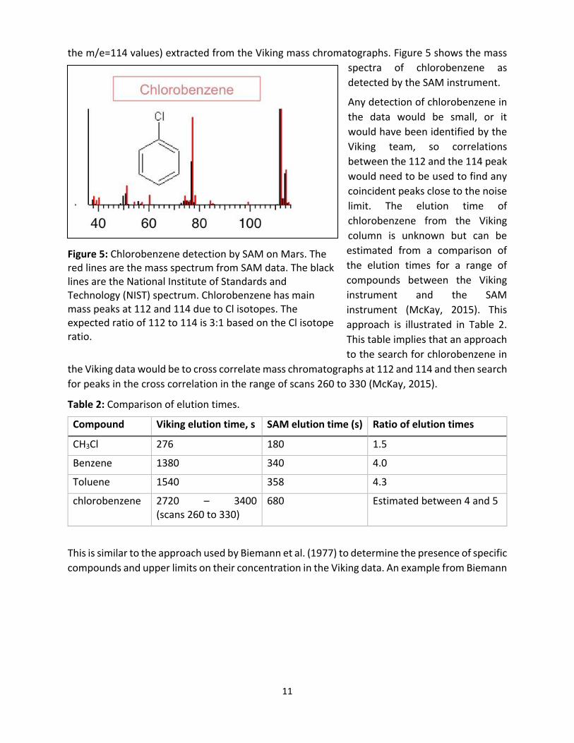
the m/e=114 values) extracted from the Viking mass chromatographs. Figure 5 shows the mass
spectra of chlorobenzene as
detected by the SAM instrument.
Any detection of chlorobenzene in
the data would be small, or it
would have been identified by the
Viking team, so correlations
between the 112 and the 114 peak
would need to be used to find any
coincident peaks close to the noise
limit. The elution time of
chlorobenzene from the Viking
column is unknown but can be
estimated from a comparison of
the elution times for a range of
compounds between the Viking
instrument and the SAM
instrument (McKay, 2015). This
approach is illustrated in Table 2.
This table implies that an approach
to the search for chlorobenzene in
the Viking data would be to cross correlate mass chromatographs at 112 and 114 and then search
for peaks in the cross correlation in the range of scans 260 to 330 (McKay, 2015).
Table 2: Comparison of elution times.
Compound Viking elution time, s SAM elution time (s) Ratio of elution times
CH3Cl 276 180 1.5
Benzene 1380 340 4.0
Toluene 1540 358 4.3
chlorobenzene 2720 – 3400 (scans 260 to 330)
680 Estimated between 4 and 5
This is similar to the approach used by Biemann et al. (1977) to determine the presence of specific
compounds and upper limits on their concentration in the Viking data. An example from Biemann
Figure 5: Chlorobenzene detection by SAM on Mars. The red lines are the mass spectrum from SAM data. The black lines are the National Institute of Standards and Technology (NIST) spectrum. Chlorobenzene has main mass peaks at 112 and 114 due to Cl isotopes. The expected ratio of 112 to 114 is 3:1 based on the Cl isotope ratio.
12
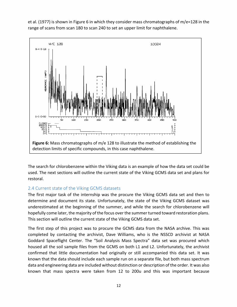
et al. (1977) is shown in Figure 6 in which they consider mass chromatographs of m/e=128 in the
range of scans from scan 180 to scan 240 to set an upper limit for naphthalene.
The search for chlorobenzene within the Viking data is an example of how the data set could be
used. The next sections will outline the current state of the Viking GCMS data set and plans for
restoral.
2.4 Current state of the Viking GCMS datasets The first major task of the internship was the procure the Viking GCMS data set and then to
determine and document its state. Unfortunately, the state of the Viking GCMS dataset was
underestimated at the beginning of the summer, and while the search for chlorobenzene will
hopefully come later, the majority of the focus over the summer turned toward restoration plans.
This section will outline the current state of the Viking GCMS data set.
The first step of this project was to procure the GCMS data from the NASA archive. This was
completed by contacting the archivist, Dave Williams, who is the NSSCD archivist at NASA
Goddard Spaceflight Center. The “Soil Analysis Mass Spectra” data set was procured which
housed all the soil sample files from the GCMS on both L1 and L2. Unfortunately, the archivist
confirmed that little documentation had originally or still accompanied this data set. It was
known that the data should include each sample run on a separate file, but both mass spectrum
data and engineering data are included without distinction or description of the order. It was also
known that mass spectra were taken from 12 to 200u and this was important because
Figure 6: Mass chromatographs of m/e 128 to illustrate the method of establishing the detection limits of specific compounds, in this case naphthalene.
13
chlorobenzene does fall within this range and would be useful for the analysis described in 2.3
Applications of Restored Viking Data.
The GCMS data currently exists in three forms.
1) Raw form on IBM-compatible tapes,
2) Presented as bar graphs on 16-mm microfilm,
3) Full and reduced versions of the data stored in files of .phys extension.
The following information was procured from a combination of reading official documentation
of the data set, a correspondence with the NSSDC archivist, and an independent analysis which
will be described in Section 2.5.
The IBM-compatible tapes are stored as they were received by the Viking experimenters from
the telemetry documentation program output, except they have been put in logical order and
gaps have been filled. The microfilm presents the same data as the tapes (Williams, 2014). The
third form, the reduced version, is the most usable to anyone not very familiar with the specific
mission operations and the instrument design.
The data is stored in 32 .phys files in binary form. The data files are split between four folders:
two folders include all sampling data while two folders include reduced versions of that same
data. Each sample run is on a separate file, and there is one record for each spectral scan,
including mass spectrum data and engineering data. Documentation is not available to delineate
bytes within a file or a group of sample files. There is no data set catalog with information to give
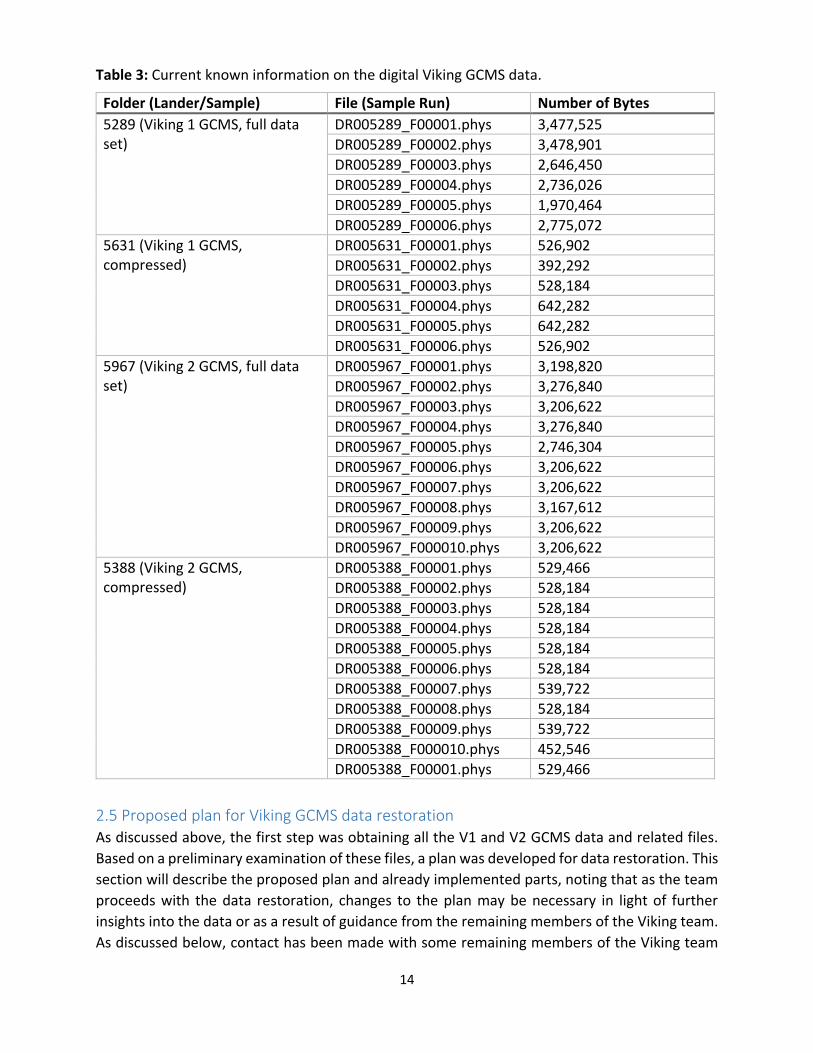
details on the formats, units, etc (Williams, 2015). Table 3 shows the known breakdown and the
size of each file.
Due to the unreadable state of the data set, it was determined that a plan for restoral should be
developed and documented for a proposal for funding from NASA Headquarters. The next section
will outline the proposed plan for restoral.
14
Table 3: Current known information on the digital Viking GCMS data.
Folder (Lander/Sample) File (Sample Run) Number of Bytes
5289 (Viking 1 GCMS, full data set)
DR005289_F00001.phys 3,477,525
DR005289_F00002.phys 3,478,901
DR005289_F00003.phys 2,646,450
DR005289_F00004.phys 2,736,026
DR005289_F00005.phys 1,970,464
DR005289_F00006.phys 2,775,072
5631 (Viking 1 GCMS, compressed)
DR005631_F00001.phys 526,902
DR005631_F00002.phys 392,292
DR005631_F00003.phys 528,184
DR005631_F00004.phys 642,282
DR005631_F00005.phys 642,282
DR005631_F00006.phys 526,902
5967 (Viking 2 GCMS, full data set)
DR005967_F00001.phys 3,198,820
DR005967_F00002.phys 3,276,840
DR005967_F00003.phys 3,206,622
DR005967_F00004.phys 3,276,840
DR005967_F00005.phys 2,746,304
DR005967_F00006.phys 3,206,622
DR005967_F00007.phys 3,206,622
DR005967_F00008.phys 3,167,612
DR005967_F00009.phys 3,206,622
DR005967_F000010.phys 3,206,622
5388 (Viking 2 GCMS, compressed)
DR005388_F00001.phys 529,466
DR005388_F00002.phys 528,184
DR005388_F00003.phys 528,184
DR005388_F00004.phys 528,184
DR005388_F00005.phys 528,184
DR005388_F00006.phys 528,184
DR005388_F00007.phys 539,722
DR005388_F00008.phys 528,184
DR005388_F00009.phys 539,722
DR005388_F000010.phys 452,546
DR005388_F00001.phys 529,466
2.5 Proposed plan for Viking GCMS data restoration As discussed above, the first step was obtaining all the V1 and V2 GCMS data and related files.
Based on a preliminary examination of these files, a plan was developed for data restoration. This
section will describe the proposed plan and already implemented parts, noting that as the team
proceeds with the data restoration, changes to the plan may be necessary in light of further
insights into the data or as a result of guidance from the remaining members of the Viking team.
As discussed below, contact has been made with some remaining members of the Viking team
15
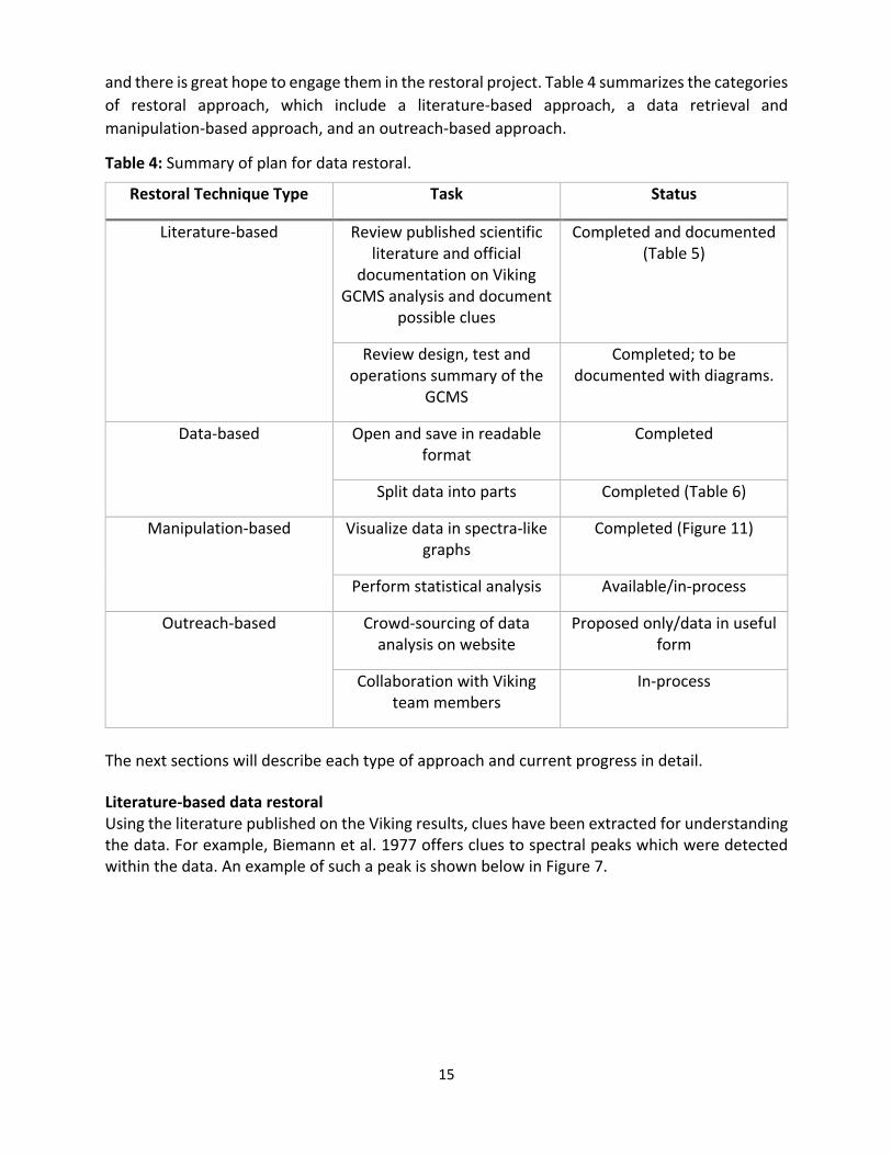
and there is great hope to engage them in the restoral project. Table 4 summarizes the categories
of restoral approach, which include a literature-based approach, a data retrieval and
manipulation-based approach, and an outreach-based approach.
Table 4: Summary of plan for data restoral.
Restoral Technique Type Task Status
Literature-based Review published scientific literature and official
documentation on Viking GCMS analysis and document
possible clues
Completed and documented (Table 5)
Review design, test and operations summary of the
GCMS
Completed; to be documented with diagrams.
Data-based
Open and save in readable format
Completed
Split data into parts Completed (Table 6)
Manipulation-based
Visualize data in spectra-like graphs
Completed (Figure 11)
Perform statistical analysis Available/in-process
Outreach-based
Crowd-sourcing of data analysis on website
Proposed only/data in useful form
Collaboration with Viking team members
In-process
The next sections will describe each type of approach and current progress in detail.
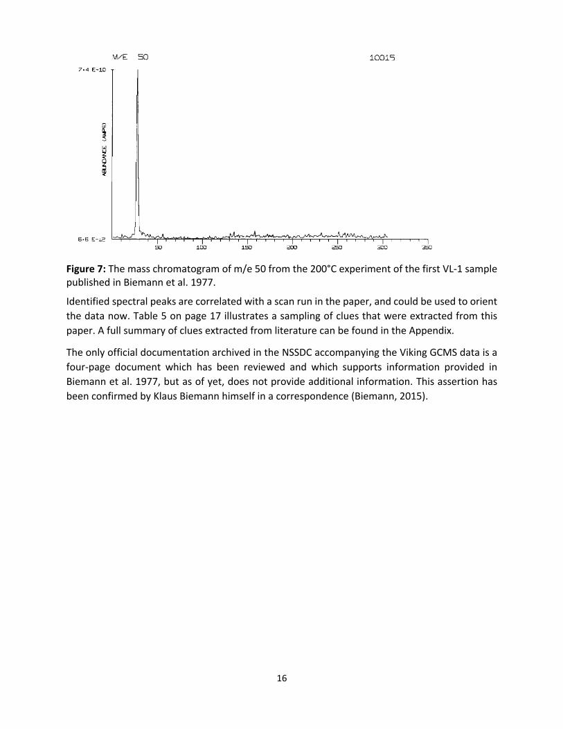
Literature-based data restoral Using the literature published on the Viking results, clues have been extracted for understanding the data. For example, Biemann et al. 1977 offers clues to spectral peaks which were detected within the data. An example of such a peak is shown below in Figure 7.
16
Figure 7: The mass chromatogram of m/e 50 from the 200°C experiment of the first VL-1 sample published in Biemann et al. 1977.
Identified spectral peaks are correlated with a scan run in the paper, and could be used to orient
the data now. Table 5 on page 17 illustrates a sampling of clues that were extracted from this
paper. A full summary of clues extracted from literature can be found in the Appendix.
The only official documentation archived in the NSSDC accompanying the Viking GCMS data is a
four-page document which has been reviewed and which supports information provided in
Biemann et al. 1977, but as of yet, does not provide additional information. This assertion has
been confirmed by Klaus Biemann himself in a correspondence (Biemann, 2015).
17
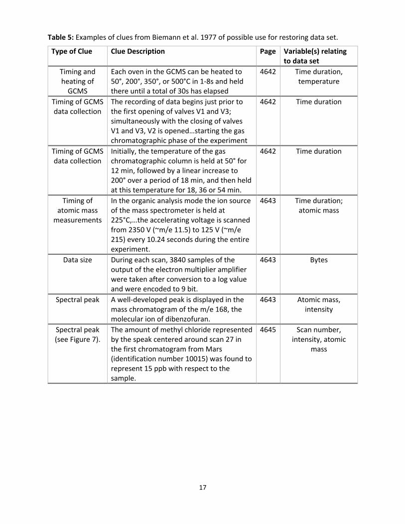
Table 5: Examples of clues from Biemann et al. 1977 of possible use for restoring data set.
Type of Clue Clue Description Page Variable(s) relating to data set
Timing and heating of
GCMS
Each oven in the GCMS can be heated to 50°, 200°, 350°, or 500°C in 1-8s and held there until a total of 30s has elapsed
4642 Time duration, temperature
Timing of GCMS data collection
The recording of data begins just prior to the first opening of valves V1 and V3; simultaneously with the closing of valves V1 and V3, V2 is opened…starting the gas chromatographic phase of the experiment
4642 Time duration
Timing of GCMS data collection
Initially, the temperature of the gas chromatographic column is held at 50° for 12 min, followed by a linear increase to 200° over a period of 18 min, and then held at this temperature for 18, 36 or 54 min.
4642 Time duration
Timing of atomic mass
measurements
In the organic analysis mode the ion source of the mass spectrometer is held at 225°C,…the accelerating voltage is scanned from 2350 V (~m/e 11.5) to 125 V (~m/e 215) every 10.24 seconds during the entire experiment.
4643 Time duration; atomic mass
Data size During each scan, 3840 samples of the output of the electron multiplier amplifier were taken after conversion to a log value and were encoded to 9 bit.
4643 Bytes
Spectral peak A well-developed peak is displayed in the mass chromatogram of the m/e 168, the molecular ion of dibenzofuran.
4643 Atomic mass, intensity
Spectral peak (see Figure 7).
The amount of methyl chloride represented by the speak centered around scan 27 in the first chromatogram from Mars (identification number 10015) was found to represent 15 ppb with respect to the sample.
4645 Scan number, intensity, atomic
mass
18
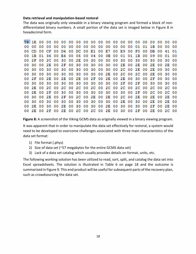
Data retrieval and manipulation-based restoral The data was originally only viewable in a binary viewing program and formed a block of non-differentiated binary numbers. A small portion of the data set is imaged below in Figure 8 in hexadecimal form.
Figure 8: A screenshot of the Viking GCMS data as originally viewed in a binary viewing program.
It was apparent that in order to manipulate the data set effectively for restoral, a system would
need to be developed to overcome challenges associated with three main characteristics of the
data set format:
1) File format (.phys)
2) Size of data set (~57 megabytes for the entire GCMS data set)
3) Lack of a data set catalog which usually provides details on format, units, etc.
The following working solution has been utilized to read, sort, split, and catalog the data set into
Excel spreadsheets. The solution is illustrated in Table 6 on page 18 and the outcome is
summarized in Figure 9. This end product will be useful for subsequent parts of the recovery plan,
such as crowdsourcing the data set.
19
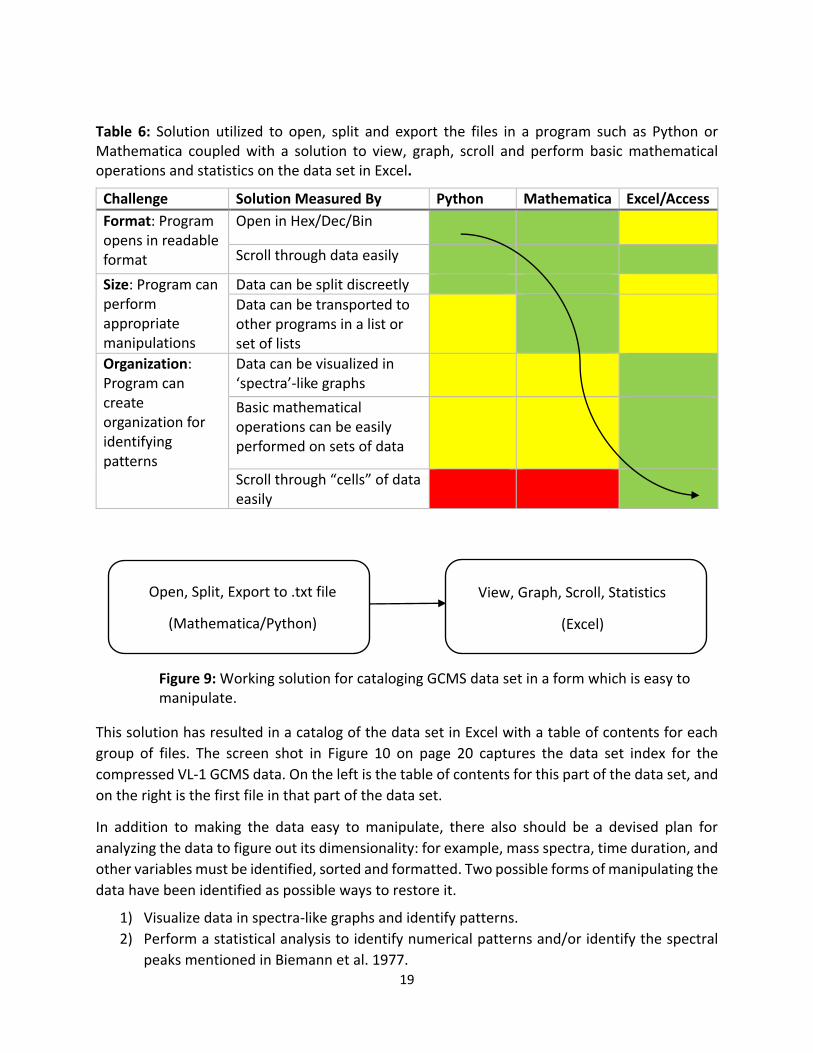
Table 6: Solution utilized to open, split and export the files in a program such as Python or Mathematica coupled with a solution to view, graph, scroll and perform basic mathematical operations and statistics on the data set in Excel.
Challenge Solution Measured By Python Mathematica Excel/Access
Format: Program opens in readable format
Open in Hex/Dec/Bin
Scroll through data easily
Size: Program can perform appropriate manipulations
Data can be split discreetly
Data can be transported to other programs in a list or set of lists
Organization: Program can create organization for identifying patterns
Data can be visualized in ‘spectra’-like graphs
Basic mathematical operations can be easily performed on sets of data
Scroll through “cells” of data easily
This solution has resulted in a catalog of the data set in Excel with a table of contents for each
group of files. The screen shot in Figure 10 on page 20 captures the data set index for the
compressed VL-1 GCMS data. On the left is the table of contents for this part of the data set, and
on the right is the first file in that part of the data set.
In addition to making the data easy to manipulate, there also should be a devised plan for
analyzing the data to figure out its dimensionality: for example, mass spectra, time duration, and
other variables must be identified, sorted and formatted. Two possible forms of manipulating the
data have been identified as possible ways to restore it.
1) Visualize data in spectra-like graphs and identify patterns.
2) Perform a statistical analysis to identify numerical patterns and/or identify the spectral
peaks mentioned in Biemann et al. 1977.
Open, Split, Export to .txt file
(Mathematica/Python)
View, Graph, Scroll, Statistics
(Excel)
Figure 9: Working solution for cataloging GCMS data set in a form which is easy to manipulate.
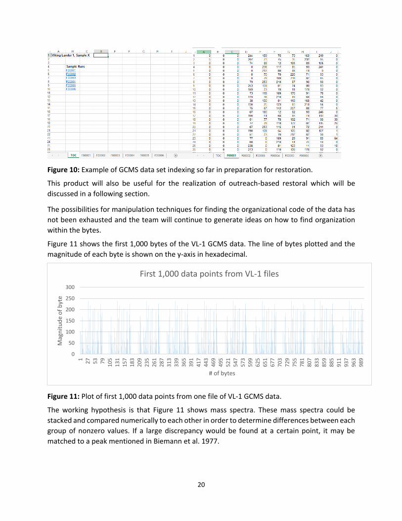
20
Figure 10: Example of GCMS data set indexing so far in preparation for restoration.
This product will also be useful for the realization of outreach-based restoral which will be
discussed in a following section.
The possibilities for manipulation techniques for finding the organizational code of the data has
not been exhausted and the team will continue to generate ideas on how to find organization
within the bytes.
Figure 11 shows the first 1,000 bytes of the VL-1 GCMS data. The line of bytes plotted and the
magnitude of each byte is shown on the y-axis in hexadecimal.
Figure 11: Plot of first 1,000 data points from one file of VL-1 GCMS data.
The working hypothesis is that Figure 11 shows mass spectra. These mass spectra could be
stacked and compared numerically to each other in order to determine differences between each
group of nonzero values. If a large discrepancy would be found at a certain point, it may be
matched to a peak mentioned in Biemann et al. 1977.
0
50
100
150
200
250
300
12
75
37
91
05
13
11
57
18
32
09
23
52
61
28
73
13
33
93
65
39
14
17
44
34
69
49
55
21
54
75
73
59
96
25
65
16
77
70
37
29
75
57
81
80
78
33
85
98
85
91
19
37
96
39
89
Mag
nit
ud
e o
f b
yte
# of bytes
First 1,000 data points from VL-1 files
21
Outreach-based restoral Because the data set is so voluminous and possibly dimensional (time-dependency, mass-dependency, dependency on the effluent divider, etc.), a parallel technique for restoration will be to make the data set available on-line and to involve and target members of the community to help look at it and analyze its patterns. The team will explore options for setting up an interactive, intuitive and robust platform for involving users in the data manipulation. Tools being explored for the purpose of crowdsourcing and sharing analysis of the data set,
currently include but are not limited to the following on-line platforms.
1) Apache Spark
2) iPython notebook
3) Zoho or Google Cloud
4) Silk
5) GitHub
In addition to involving interested public users, the team has also invested effort into contacting,
involving and collaborating with members of the original Viking team and other knowledgeable
persons, and will continue to do so.
The team has already benefitted from communication with the following people, and will
continue to seek collaboration and support.
1) Dave Williams, Planetary Curation Scientist, National Space Science Data Center, NASA Goddard Space Flight Center.
2) Klaus Biemann, Principle Investigator of the Viking GCMS, Professor Emeritus of
Chemistry at the Massachusetts Institute of Technology.
3) Rachel Tillman, Founder and Director of The Viking Mars Missions Education and
Preservation Project, owner of original MDR tapes from the Viking mission.
These ongoing communications have emphasized that many people are interested and engaged
in Viking data restoral. Reaching out to and utilizing that community will only help the goals and
vision of this Viking GCMS restoral project. Although only a few members of the original Viking
team still remain, these members and other interested, knowledgeable parties are still engaged
and working to keep the Viking data available and useful.
2.6 Submission of PDART proposal and future plans The team successfully submitted a proposal for restoration of the Viking GCMS data set on Friday July 17 to the Planetary Data Archiving, Restoration, and Tools (PDART) program of NASA Headquarters. This program solicits proposals to generate data products, archive and restore data sets, create or consolidate reference databases, or generate new information, digitize data, or develop software tools for data sets (NASA Headquarters, 2009). Most of the information provided in that proposal is also provided in this report. If this proposal is approved, the team will received funding for a full calendar year and will continue to restore the Viking data set through the proposed plan outlined in Section 2.5.
22
3. Modelling perceived temperature of the human body on other planets This section will outline the objectives, methodology, background work, completed analysis and
the current status of the initiative to model the perceived temperature of the human body while
standing on the surface of Mars, Titan, or Europa.
3.1 Perceived Temperature Objectives After the successful submission of the PDART proposal in late July, the focus of the internship
shifted to a secondary project. There would be an interim wait period of months to hear back on
the status of the Viking proposal. The secondary project is to create a thermal model to
determine the comfort for a human standing on the surface of Mars, Titan, and Europa.
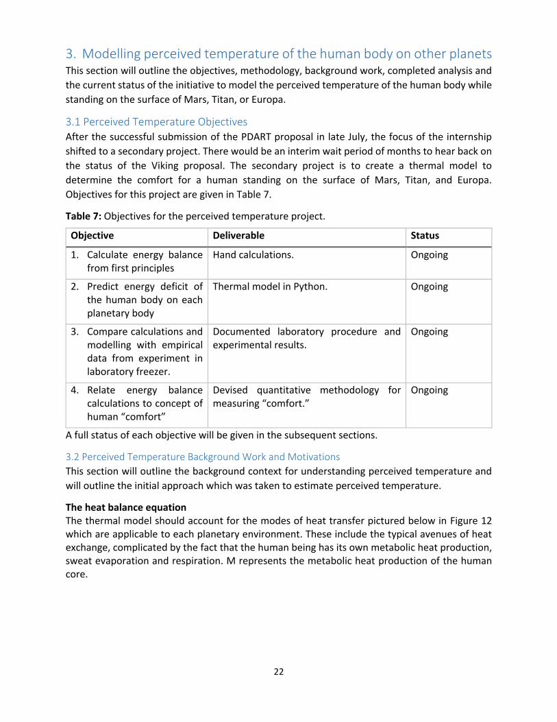
Objectives for this project are given in Table 7.
Table 7: Objectives for the perceived temperature project.
Objective Deliverable Status
1. Calculate energy balance from first principles
Hand calculations. Ongoing
2. Predict energy deficit of the human body on each planetary body
Thermal model in Python. Ongoing
3. Compare calculations and modelling with empirical data from experiment in laboratory freezer.
Documented laboratory procedure and experimental results.
Ongoing
4. Relate energy balance calculations to concept of human “comfort”
Devised quantitative methodology for measuring “comfort.”
Ongoing
A full status of each objective will be given in the subsequent sections.
3.2 Perceived Temperature Background Work and Motivations
This section will outline the background context for understanding perceived temperature and
will outline the initial approach which was taken to estimate perceived temperature.
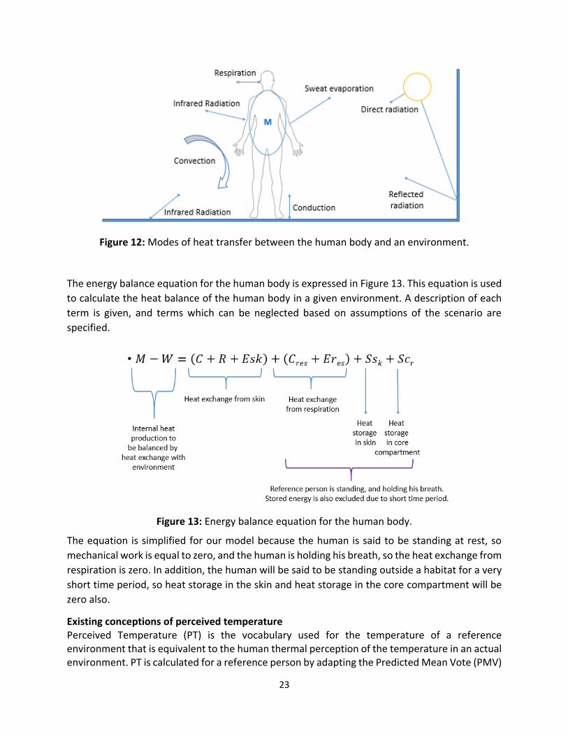
The heat balance equation The thermal model should account for the modes of heat transfer pictured below in Figure 12 which are applicable to each planetary environment. These include the typical avenues of heat exchange, complicated by the fact that the human being has its own metabolic heat production, sweat evaporation and respiration. M represents the metabolic heat production of the human core.
23
Figure 12: Modes of heat transfer between the human body and an environment.
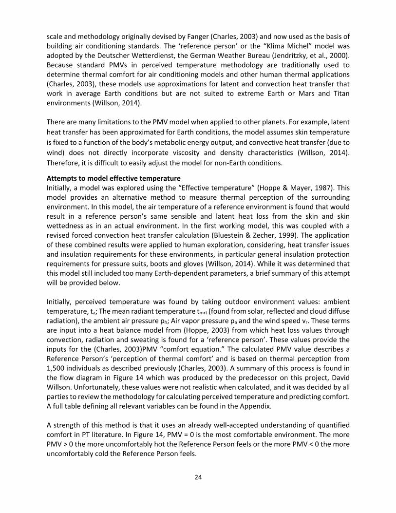
The energy balance equation for the human body is expressed in Figure 13. This equation is used
to calculate the heat balance of the human body in a given environment. A description of each
term is given, and terms which can be neglected based on assumptions of the scenario are
specified.
Figure 13: Energy balance equation for the human body.
The equation is simplified for our model because the human is said to be standing at rest, so
mechanical work is equal to zero, and the human is holding his breath, so the heat exchange from
respiration is zero. In addition, the human will be said to be standing outside a habitat for a very
short time period, so heat storage in the skin and heat storage in the core compartment will be
zero also.
Existing conceptions of perceived temperature Perceived Temperature (PT) is the vocabulary used for the temperature of a reference environment that is equivalent to the human thermal perception of the temperature in an actual environment. PT is calculated for a reference person by adapting the Predicted Mean Vote (PMV)
24
scale and methodology originally devised by Fanger (Charles, 2003) and now used as the basis of building air conditioning standards. The ‘reference person’ or the “Klima Michel” model was adopted by the Deutscher Wetterdienst, the German Weather Bureau (Jendritzky, et al., 2000). Because standard PMVs in perceived temperature methodology are traditionally used to determine thermal comfort for air conditioning models and other human thermal applications (Charles, 2003), these models use approximations for latent and convection heat transfer that work in average Earth conditions but are not suited to extreme Earth or Mars and Titan environments (Willson, 2014). There are many limitations to the PMV model when applied to other planets. For example, latent
heat transfer has been approximated for Earth conditions, the model assumes skin temperature
is fixed to a function of the body’s metabolic energy output, and convective heat transfer (due to
wind) does not directly incorporate viscosity and density characteristics (Willson, 2014).
Therefore, it is difficult to easily adjust the model for non-Earth conditions.
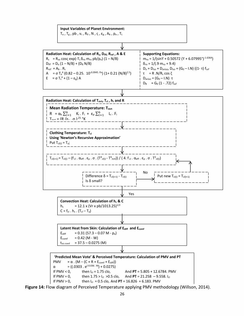
Attempts to model effective temperature Initially, a model was explored using the “Effective temperature” (Hoppe & Mayer, 1987). This model provides an alternative method to measure thermal perception of the surrounding environment. In this model, the air temperature of a reference environment is found that would result in a reference person’s same sensible and latent heat loss from the skin and skin wettedness as in an actual environment. In the first working model, this was coupled with a revised forced convection heat transfer calculation (Bluestein & Zecher, 1999). The application of these combined results were applied to human exploration, considering, heat transfer issues and insulation requirements for these environments, in particular general insulation protection requirements for pressure suits, boots and gloves (Willson, 2014). While it was determined that this model still included too many Earth-dependent parameters, a brief summary of this attempt will be provided below. Initially, perceived temperature was found by taking outdoor environment values: ambient temperature, ta; The mean radiant temperature tmrt (found from solar, reflected and cloud diffuse radiation), the ambient air pressure ph; Air vapor pressure pa and the wind speed vr. These terms are input into a heat balance model from (Hoppe, 2003) from which heat loss values through convection, radiation and sweating is found for a ‘reference person’. These values provide the inputs for the (Charles, 2003)PMV “comfort equation.” The calculated PMV value describes a Reference Person’s ‘perception of thermal comfort’ and is based on thermal perception from 1,500 individuals as described previously (Charles, 2003). A summary of this process is found in the flow diagram in Figure 14 which was produced by the predecessor on this project, David Willson. Unfortunately, these values were not realistic when calculated, and it was decided by all parties to review the methodology for calculating perceived temperature and predicting comfort. A full table defining all relevant variables can be found in the Appendix. A strength of this method is that it uses an already well-accepted understanding of quantified comfort in PT literature. In Figure 14, PMV = 0 is the most comfortable environment. The more PMV > 0 the more uncomfortably hot the Reference Person feels or the more PMV < 0 the more uncomfortably cold the Reference Person feels.
25
3.3 Mojave Desert field measurements In the last section, Figure 14 described initial attempts to quantify perceived temperature.
However, it was found that this model still had too many Earth-related parameters and was
producing unrealistic estimates of temperature. It was decided to calculate energy balance from
first principles and then to develop a method for relating these energy balances to human
comfort. This section will cover the field measurements that were taken and utilized for initial
calculations of energy balance from first principles.
Field measurements were taken in the Mojave Desert at two different sites in order to make
calculations of energy balance for the human body. These empirical measurements could be used
for first principle calculations and could be compared to numerical or theoretical values.
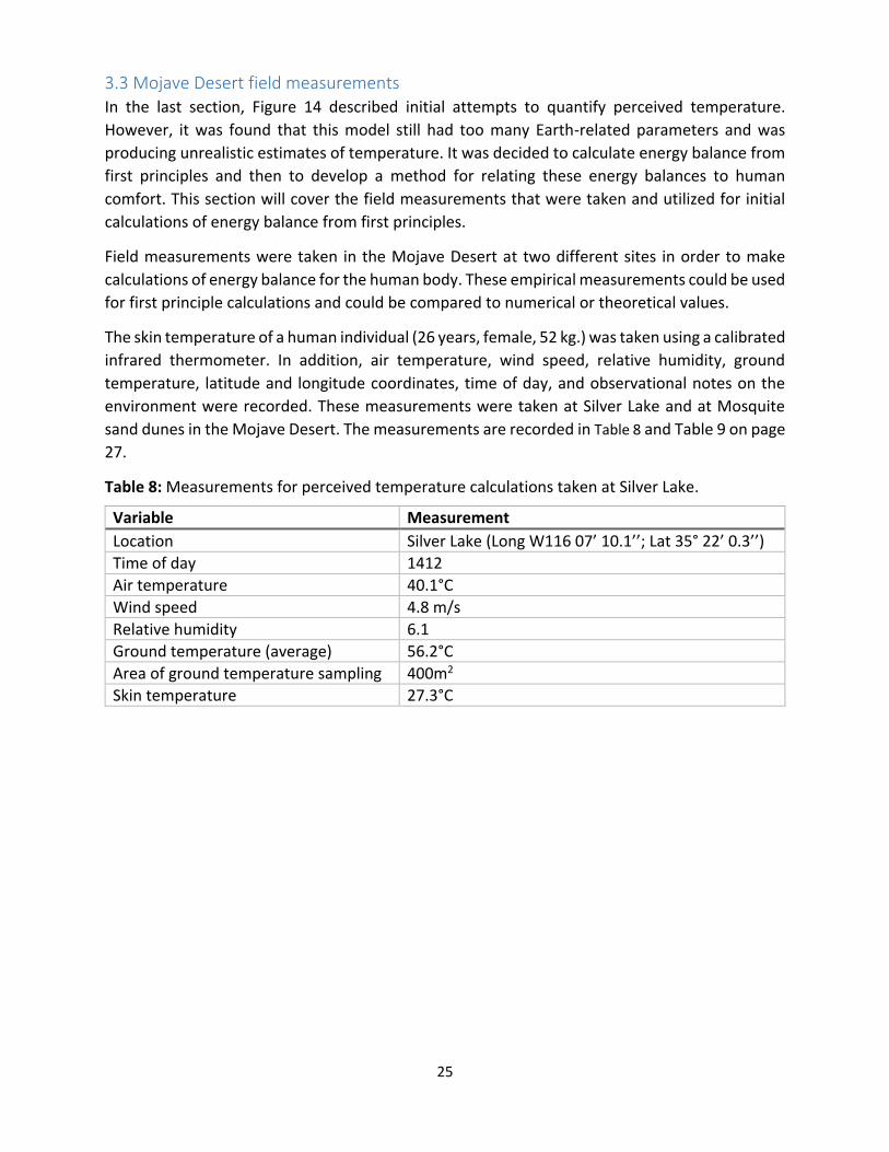
The skin temperature of a human individual (26 years, female, 52 kg.) was taken using a calibrated
infrared thermometer. In addition, air temperature, wind speed, relative humidity, ground
temperature, latitude and longitude coordinates, time of day, and observational notes on the
environment were recorded. These measurements were taken at Silver Lake and at Mosquite
sand dunes in the Mojave Desert. The measurements are recorded in Table 8 and Table 9 on page
27.
Table 8: Measurements for perceived temperature calculations taken at Silver Lake.
Variable Measurement
Location Silver Lake (Long W116 07’ 10.1’’; Lat 35° 22’ 0.3’’)
Time of day 1412
Air temperature 40.1°C
Wind speed 4.8 m/s
Relative humidity 6.1
Ground temperature (average) 56.2°C
Area of ground temperature sampling 400m2
Skin temperature 27.3°C
26
Radiation Heat: Calculation of Tmrt, Tcl , hr and R
Tcl(i+1) = Tcl(i) – (f cl . αeff . εp . σ . (T4cl(i) - T4
mrt)) / ( 4. f cl . αeff . εp . σ . T3cl(i))
Difference δ = Tcl(i+1) - Tcl(i) Is δ small?
Put new Tcl(i) = Tcl(I+1)
Mean Radiation Temperature: Tmrt
R = αk ∑6𝑖=1 Ki . Fi + εp ∑6
𝑖=1 Li . Fi Tmrt = (R /εs . σ.).25 °K
Clothing Temperature: Tcl Using ‘Newton’s Recursive Approximation’ Put Tcl(i) = Ta;
Convection Heat: Calculation of hc & C hc = 12.1 x (Vr x pb/1013.25)1/2 C = fcl . hc . (Tcl – Ta)
Latent Heat from Skin: Calculation of Ediff and Ecomf Ediff = 0.31 (57.3 – 0.07 M - pa) Ecomf = 0.42 (M - W) tsk,comf = 37.5 – 0.0275 (M)
‘Predicted Mean Vote’ & Perceived Temperature: Calculation of PMV and PT PMV = α . (M – (C + R + Ecomf + Ediff)) α = ((.0303 . e(-0.036 . M) + 0.0275) If PMV < 0, then Icl = 1.75 clo, And PT = 5.805 + 12.6784. PMV If PMV = 0, then 1.75 > Icl >0.5 clo, And PT = 21.258 – 9.558. Icl If PMV > 0, then Icl = 0.5 clo, And PT = 16.826 + 6.183. PMV
Radiation Heat: Calculation of Rs, Diff, Rref , A & E Rs = Rso cosς exp(-TL δro mro pb/po) (1 – N/8) Diff = Do (1 – N/8) + (D8 N/8) Rref = Ab . Rs A = σ Ta
4 (0.82 – 0.25. 10-0.0945. Pa) (1+ 0.21 (N/8)2.5) E = σ Ts
4 + (1 – εg) A
No
Yes
Supporting Equations: mro = 1/(sinϒ + 0.50572 (ϒ + 6.07995°)-1.6364) δro = 1/(.9 mro + 9.4) Do = Diso + Daniso, Diso = (G0 – I.N) ((1- τ) fsvf τ = R .N/Rs cos ζ Daniso = (G0 – I.N) τ D8 = G0 (1 - .72) fsvf
Input Variables of Planet Environment: Ta , Tg , pb , vr , R0 , N , ς , εg , Ab , pa , TL
Figure 14: Flow diagram of Perceived Temperature applying PMV methodology (Willson, 2014).
27
Table 9: Measurements for perceived temperature calculations taken at Mosquite sand dunes.
Variable Measurement
Location Mosquite sand dunes (N 36°36’26’’; W117 6’53’’)
Time of day 950
Air temperature 40.6°C
Wind speed 0 – 0.9 m/s
Relative humidity 10.9
Ground temperature (average) 51.2°C
Area of ground temperature sampling 400m2
Skin temperature 35.4°C
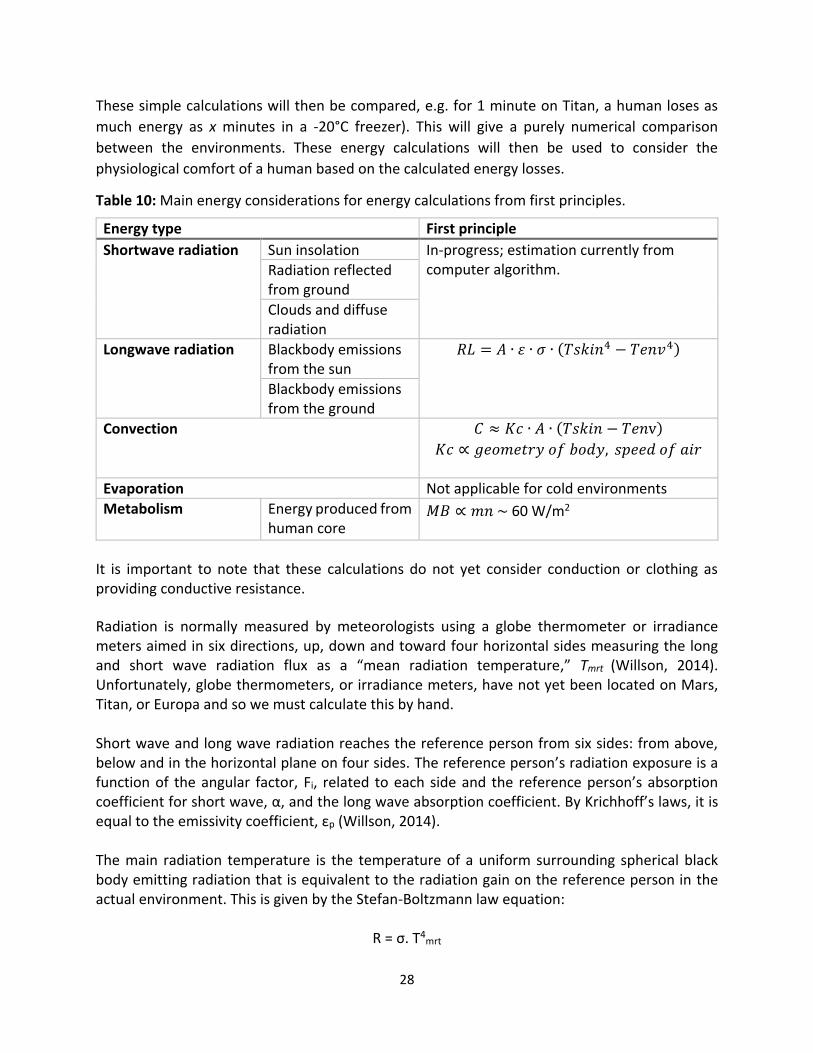
Figure 15 depicts the lab subject during skin temperature readings to the left. The right image in
Figure 15 depicts the type of desert environment which was ideal for measurements, given its
flat surface, low cloud cover, and negligible vegetation.
Figure 15: Images of field measurement locations and test subject in the Mojave Desert.
These empirical measurements have been used for back-of-the-envelope calculations of energy
balance, described in the next section.
3.4 Plan of action for perceived temperature future progress As this report goes to print, there is still two weeks remaining of the internship and a probable
extension of the projects’ duration. The next section will cover the plan of action from this point.
Energy calculations from first principles Using the -20°C walk-in freezer in the Space Sciences building at NASA Ames, the energy loss of a human test subject will be calculated. Energy loss for a human being on Mars, Titan and Europa will also be calculated from first principles. The components which will be considered in these calculations are outlined in Table 10.
28
These simple calculations will then be compared, e.g. for 1 minute on Titan, a human loses as
much energy as x minutes in a -20°C freezer). This will give a purely numerical comparison
between the environments. These energy calculations will then be used to consider the
physiological comfort of a human based on the calculated energy losses.
Table 10: Main energy considerations for energy calculations from first principles.
Energy type First principle
Shortwave radiation Sun insolation In-progress; estimation currently from computer algorithm. Radiation reflected
from ground
Clouds and diffuse radiation
Longwave radiation Blackbody emissions from the sun
𝑅𝐿 = 𝐴 ∙ 𝜀 ∙ 𝜎 ∙ (𝑇𝑠𝑘𝑖𝑛4 − 𝑇𝑒𝑛𝑣4)
Blackbody emissions from the ground
Convection 𝐶 ≈ 𝐾𝑐 ∙ 𝐴 ∙ (𝑇𝑠𝑘𝑖𝑛 − 𝑇𝑒𝑛v)
𝐾𝑐 ∝ 𝑔𝑒𝑜𝑚𝑒𝑡𝑟𝑦 𝑜𝑓 𝑏𝑜𝑑𝑦, 𝑠𝑝𝑒𝑒𝑑 𝑜𝑓 𝑎𝑖𝑟
Evaporation Not applicable for cold environments
Metabolism Energy produced from human core
𝑀𝐵 ∝ 𝑚𝑛 ~ 60 W/m2
It is important to note that these calculations do not yet consider conduction or clothing as providing conductive resistance.
Radiation is normally measured by meteorologists using a globe thermometer or irradiance meters aimed in six directions, up, down and toward four horizontal sides measuring the long and short wave radiation flux as a “mean radiation temperature,” Tmrt (Willson, 2014). Unfortunately, globe thermometers, or irradiance meters, have not yet been located on Mars, Titan, or Europa and so we must calculate this by hand. Short wave and long wave radiation reaches the reference person from six sides: from above, below and in the horizontal plane on four sides. The reference person’s radiation exposure is a function of the angular factor, Fi, related to each side and the reference person’s absorption coefficient for short wave, α, and the long wave absorption coefficient. By Krichhoff’s laws, it is equal to the emissivity coefficient, εp (Willson, 2014). The main radiation temperature is the temperature of a uniform surrounding spherical black body emitting radiation that is equivalent to the radiation gain on the reference person in the actual environment. This is given by the Stefan-Boltzmann law equation:
R = σ. T4mrt
29
In addition, our calculation to find the radiation heat transfer coefficient hr is derived from the Stefan-Boltzmann law equated to a standard heat transfer equation as shown by the following calculation.
R = fcl . αeff . εp . σ . (T4cl - T4
mrt) = fcl . hr . (Tcl – Tmrt) W/m2
That is the radiation heat transfer coefficient.
hr = αeff . εp . σ . (T4cl - T4
mrt)/ (Tcl – Tmrt) W/m2K Convective heat and the convection heat transfer coefficient hc is calculated from the standard heat transfer equation,
C = fcl . hc . (Tcl – Ta) W/m2
Where the nature of the airflow heat transfer is covered by the heat transfer coefficient hc and will need to be derived for specific environments. Specifically on Titan, we will need to consider a nitrogen-rich atmosphere.
hc = 12.1 x (vr . pb/1013.25)1/2 W/m2K
Most perceived temperature models assume ‘forced’ convection, either laminar or turbulent air flow passing around the body at all times. This is an approximation covering a range of air flows, demonstrated to be reasonably accurate for most Earth environments but not suited for Mars or Titan atmospheres. More updated heat transfer coefficient, hc, calculation methods will be better suited for Mars, Titan, Europa and extreme Earth environments (Willson, 2014).
30
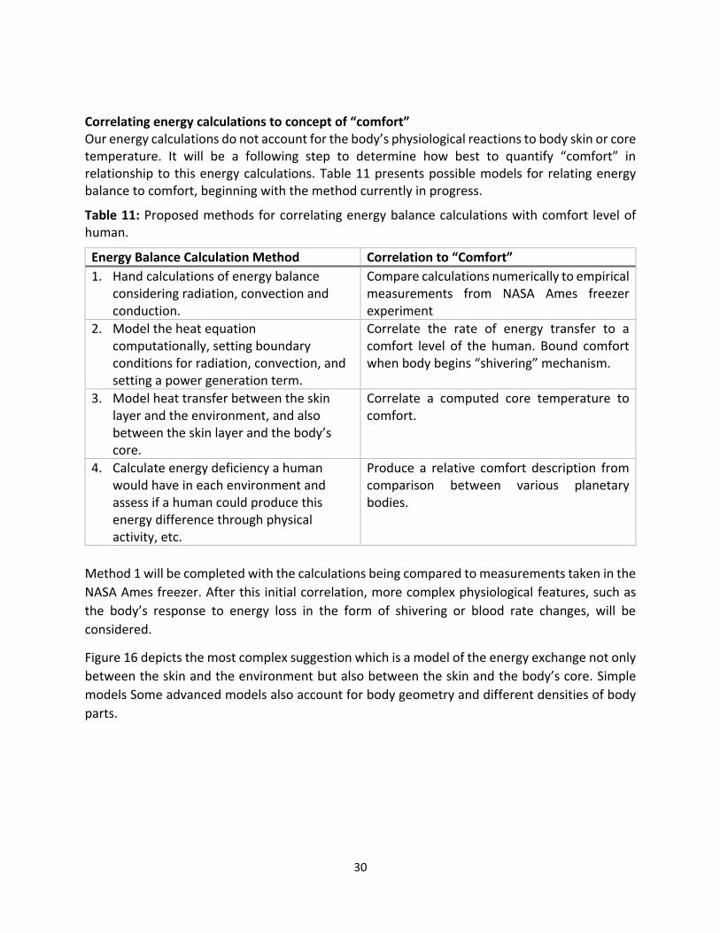
Correlating energy calculations to concept of “comfort” Our energy calculations do not account for the body’s physiological reactions to body skin or core temperature. It will be a following step to determine how best to quantify “comfort” in relationship to this energy calculations. Table 11 presents possible models for relating energy balance to comfort, beginning with the method currently in progress.
Table 11: Proposed methods for correlating energy balance calculations with comfort level of human.
Energy Balance Calculation Method Correlation to “Comfort”
1. Hand calculations of energy balance considering radiation, convection and conduction.
Compare calculations numerically to empirical measurements from NASA Ames freezer experiment
2. Model the heat equation computationally, setting boundary conditions for radiation, convection, and setting a power generation term.
Correlate the rate of energy transfer to a comfort level of the human. Bound comfort when body begins “shivering” mechanism.
3. Model heat transfer between the skin layer and the environment, and also between the skin layer and the body’s core.
Correlate a computed core temperature to comfort.
4. Calculate energy deficiency a human would have in each environment and assess if a human could produce this energy difference through physical activity, etc.
Produce a relative comfort description from comparison between various planetary bodies.
Method 1 will be completed with the calculations being compared to measurements taken in the
NASA Ames freezer. After this initial correlation, more complex physiological features, such as
the body’s response to energy loss in the form of shivering or blood rate changes, will be
considered.
Figure 16 depicts the most complex suggestion which is a model of the energy exchange not only
between the skin and the environment but also between the skin and the body’s core. Simple
models Some advanced models also account for body geometry and different densities of body
parts.
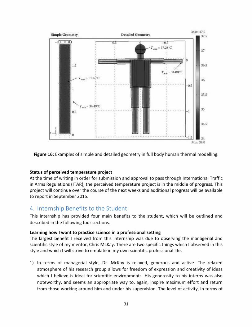
31
Figure 16: Examples of simple and detailed geometry in full body human thermal modelling.
Status of perceived temperature project At the time of writing in order for submission and approval to pass through International Traffic in Arms Regulations (ITAR), the perceived temperature project is in the middle of progress. This project will continue over the course of the next weeks and additional progress will be available to report in September 2015.
4. Internship Benefits to the Student This internship has provided four main benefits to the student, which will be outlined and
described in the following four sections.
Learning how I want to practice science in a professional setting The largest benefit I received from this internship was due to observing the managerial and scientific style of my mentor, Chris McKay. There are two specific things which I observed in this style and which I will strive to emulate in my own scientific professional life. 1) In terms of managerial style, Dr. McKay is relaxed, generous and active. The relaxed
atmosphere of his research group allows for freedom of expression and creativity of ideas
which I believe is ideal for scientific environments. His generosity to his interns was also
noteworthy, and seems an appropriate way to, again, inspire maximum effort and return
from those working around him and under his supervision. The level of activity, in terms of
32
number of projects, in his research group is also something I would like to be a part of my
further professional life. Working on different and diverse projects this summer was
challenging but enriching. Working in astrobiology is general was very exciting in this way: it’s
a field where understanding the biology, chemistry, physics and geology can all be important
to a specific research question.
2) In terms of his approach to scientific questions, Dr. McKay is curious, creative, and has a very
interesting combination of using first principles and brute force in his approaches. He refers
naturally to first principles when a project is stuck, but also has intuition to how measures
can be estimated. It’s a rare combination of the physicist and the engineer, and I have not
often noticed this combination in a professional approach. He is constantly generating
innovative ideas which still keep sight of the bigger picture, whether it’s a bigger picture
mandated by physics or the bigger picture mandated by government.
Before I came to this internship, I worried about feeling at place within the NASA system or within
a professional environment in general. It seemed that the bureaucracy may override any purely
scientific joy I experienced. However, Dr. McKay’s research group felt quite the opposite from
this and I felt assured that there are potential places within the scientific community where
curiosity, first principles, and scientific results, positive or negative, with applications for the real
world are still at the heart of professional life.
Future professional opportunities This internship also offered me the possibility for a professional opportunity at Ames after the internship. If the Viking GCMS restoral proposal is approved, I will be able to stay on with some funding and proceed with this project. I already feel invested in the restoral, and it will be exciting to be able to continue in a more full-time and compensated way. Dr. McKay is also exploring other project and funding opportunities for me at Ames to supplement the Viking work, and I am hopeful that I will be able to stay at Ames for the coming year. The challenges and joys of the Bay Area Living in the Bay Area was both very joyful and very challenging. Time and money are scarce for the summer intern in this place of high cost and constant traffic jams. However, even though I am American by nationality, I got to explore a completely new place and culture than I have before. The Bay Area is culturally and ethnically diverse; there are people, food and culture from everywhere in the world here. The weather is beautiful, with the sad exception of the lack of rain. It was a good experience to come here to California and experience the West Coast after having grown up most of my life on the United States’ East Coast.
5. Conclusion Two projects were the focus of this internship period: to assess the state of the Viking GCMS data and then devising a plan for its restoral and to produce a thermal model for the human on other planetary bodies.
33
The primary task for the summer was to procure the GCMS data from the National Space Science
Data Coordinated Archive (NSSDCA) and to assess the current state of the data set for possible
reanalysis opportunities. After procurement of the Viking GCMS data set and analysis of its
current state, the internship focus shifted to preparing a plan for restoral and archiving of the
GCMS data set. A proposal was prepared and submitted to NASA Headquarters to restore and
make available the 8000 mass chromatographs that are the basic data generated by the Viking
GCMS instrument. The relevance of this restoral and the methodology we propose for restoral is
presented. The results of the first project is that a proposal has been submitting to NASA
Headquarters with a continuation of the project awaiting approval and funding of this proposal.
The secondary task for the summer is to develop a thermal model for the perceived temperature
of a human standing on Mars, Titan, or Europa. Traditionally, an equation called “Fanger’s
comfort equation” is used to measure the perceived temperature by a human in a given
reference environment. However, there are limitations to this model when applied to other
planets. Therefore, the approach for this project has been to derive energy balance equations
from first principles and then develop a methodology for correlating “comfort” to energy
balance. Using the -20°C walk-in freezer in the Space Sciences building at NASA Ames, energy loss
of a human subject is measured. Energy loss for a human being on Mars, Titan and Europa are
calculated from first principles. These calculations are compared to the freezer measurements,
e.g. for 1 minute on Titan, a human loses as much energy as x minutes in a -20°C freezer. This
gives a numerical comparison between the environments. These energy calculations are used to
consider the physiological comfort of a human based on the calculated energy losses. The results
of the second project are still ongoing, with the most noteworthy current tasks being the
calculations from first principles of energy balance for a human experiencing various forms of
heat transfer, and the laboratory design and setup plan for conducting experiments and
measurements in the -20°C freezer at NASA Ames.
The following Table 12 on page 34 summarizes current gaps in the projects and recommendations for further work. For the Viking project, these recommendations include only ones that should be implemented before the PDART proposal is approved. If the Viking PDART proposal is approved, additional tasks will be implemented. For the Perceived Temperature project, some of these tasks will be implemented in the following weeks.
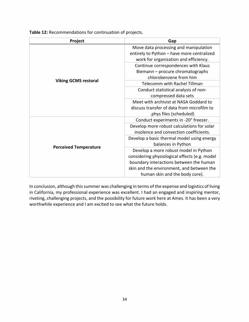
34
Table 12: Recommendations for continuation of projects.
Project Gap
Viking GCMS restoral
Move data processing and manipulation entirely to Python – have more centralized
work for organization and efficiency.
Continue correspondences with Klaus Biemann – procure chromatographs
chlorobenzene from him
Telecomm with Rachel Tillman
Conduct statistical analysis of non-compressed data sets
Meet with archivist at NASA Goddard to discuss transfer of data from microfilm to
.phys files (scheduled)
Perceived Temperature
Conduct experiments in -20° freezer.
Develop more robust calculations for solar insolence and convection coefficients.
Develop a basic thermal model using energy balances in Python
Develop a more robust model in Python considering physiological effects (e.g. model boundary interactions between the human skin and the environment, and between the
human skin and the body core).
In conclusion, although this summer was challenging in terms of the expense and logistics of living in California, my professional experience was excellent. I had an engaged and inspiring mentor, riveting, challenging projects, and the possibility for future work here at Ames. It has been a very worthwhile experience and I am excited to see what the future holds.
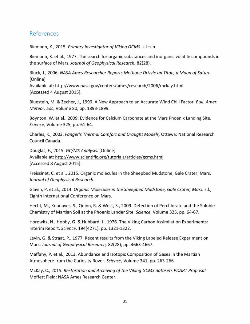
35
References
Biemann, K., 2015. Primary Investigator of Viking GCMS. s.l.:s.n.
Biemann, K. et al., 1977. The search for organic substances and inorganic volatile compounds in
the surface of Mars. Journal of Geophysical Research, 82(28).
Bluck, J., 2006. NASA Ames Researcher Reports Methane Drizzle on Titan, a Moon of Saturn.
[Online]
Available at: http://www.nasa.gov/centers/ames/research/2006/mckay.html
[Accessed 4 August 2015].
Bluestein, M. & Zecher, J., 1999. A New Approach to an Accurate Wind Chill Factor. Bull. Amer.
Meteor. Soc, Volume 80, pp. 1893-1899.
Boynton, W. et al., 2009. Evidence for Calcium Carbonate at the Mars Phoenix Landing Site.
Science, Volume 325, pp. 61-64.
Charles, K., 2003. Fanger's Thermal Comfort and Draught Models, Ottawa: National Research
Council Canada.
Douglas, F., 2015. GC/MS Analysis. [Online]
Available at: http://www.scientific.org/tutorials/articles/gcms.html
[Accessed 8 August 2015].
Freissinet, C. et al., 2015. Organic molecules in the Sheepbed Mudstone, Gale Crater, Mars.
Journal of Geophysical Research.
Glavin, P. et al., 2014. Organic Molecules in the Sheepbed Mudstone, Gale Crater, Mars. s.l.,
Eighth International Conference on Mars.
Hecht, M., Kounaves, S., Quinn, R. & West, S., 2009. Detection of Perchlorate and the Soluble
Chemistry of Martian Soil at the Phoenix Lander Site. Science, Volume 325, pp. 64-67.
Horowitz, N., Hobby, G. & Hubbard, J., 1976. The Viking Carbon Assimilation Experiments:
Interim Report. Science, 194(4271), pp. 1321-1322.
Levin, G. & Straat, P., 1977. Recent results from the Viking Labeled Release Experiment on
Mars. Journal of Geophysical Research, 82(28), pp. 4663-4667.
Maffahy, P. et al., 2013. Abundance and Isotopic Composition of Gases in the Martian
Atmosphere from the Curiosity Rover. Science, Volume 341, pp. 263-266.
McKay, C., 2015. Restoration and Archiving of the Viking GCMS datasets PDART Proposal.
Moffett Field: NASA Ames Research Center.
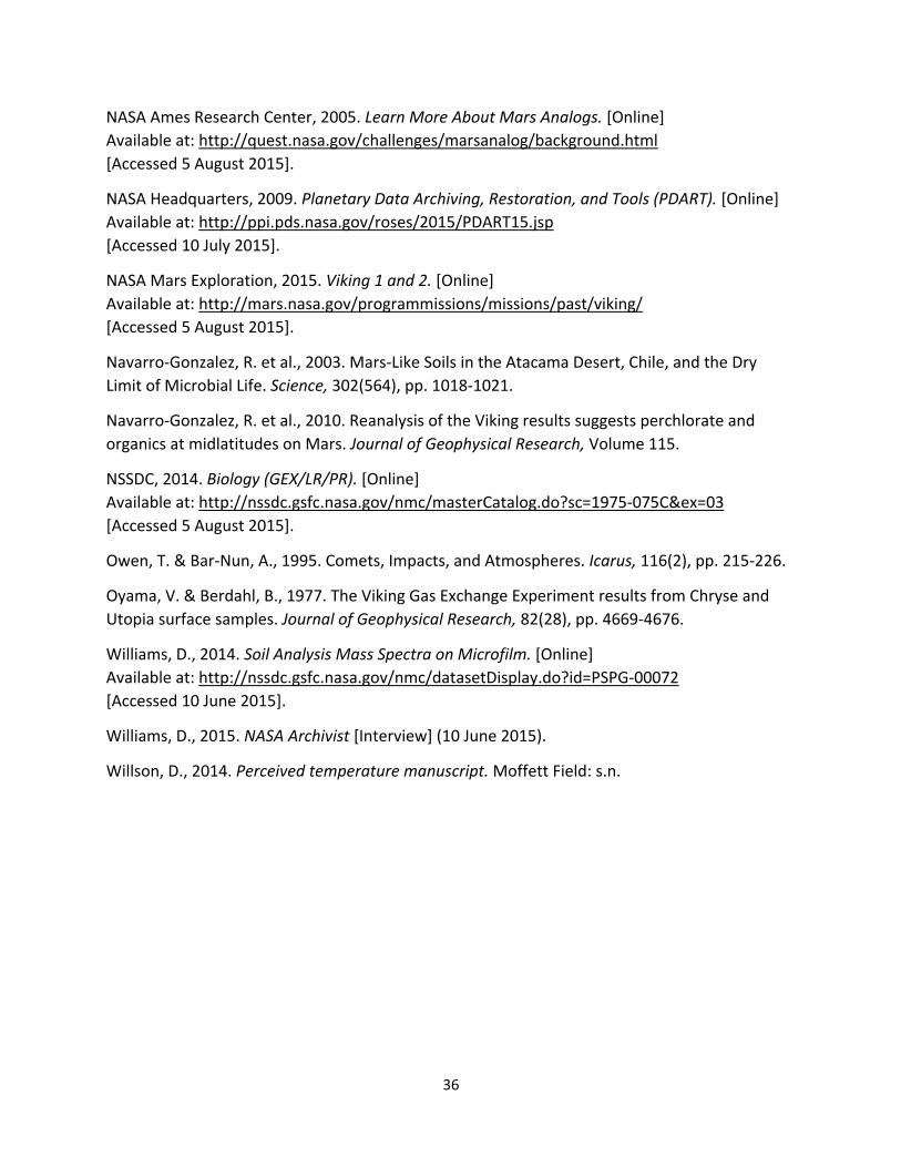
36
NASA Ames Research Center, 2005. Learn More About Mars Analogs. [Online]
Available at: http://quest.nasa.gov/challenges/marsanalog/background.html
[Accessed 5 August 2015].
NASA Headquarters, 2009. Planetary Data Archiving, Restoration, and Tools (PDART). [Online]
Available at: http://ppi.pds.nasa.gov/roses/2015/PDART15.jsp
[Accessed 10 July 2015].
NASA Mars Exploration, 2015. Viking 1 and 2. [Online]
Available at: http://mars.nasa.gov/programmissions/missions/past/viking/
[Accessed 5 August 2015].
Navarro-Gonzalez, R. et al., 2003. Mars-Like Soils in the Atacama Desert, Chile, and the Dry
Limit of Microbial Life. Science, 302(564), pp. 1018-1021.
Navarro-Gonzalez, R. et al., 2010. Reanalysis of the Viking results suggests perchlorate and
organics at midlatitudes on Mars. Journal of Geophysical Research, Volume 115.
NSSDC, 2014. Biology (GEX/LR/PR). [Online]
Available at: http://nssdc.gsfc.nasa.gov/nmc/masterCatalog.do?sc=1975-075C&ex=03
[Accessed 5 August 2015].
Owen, T. & Bar-Nun, A., 1995. Comets, Impacts, and Atmospheres. Icarus, 116(2), pp. 215-226.
Oyama, V. & Berdahl, B., 1977. The Viking Gas Exchange Experiment results from Chryse and
Utopia surface samples. Journal of Geophysical Research, 82(28), pp. 4669-4676.
Williams, D., 2014. Soil Analysis Mass Spectra on Microfilm. [Online]
Available at: http://nssdc.gsfc.nasa.gov/nmc/datasetDisplay.do?id=PSPG-00072
[Accessed 10 June 2015].
Williams, D., 2015. NASA Archivist [Interview] (10 June 2015).
Willson, D., 2014. Perceived temperature manuscript. Moffett Field: s.n.
37
Appendix
Table 13: Full document of clues from Biemann et al. 1977.
Type of Clue Clue Description Page number
Variable(s) relating to data set
Timing and heating of GCMS
Each oven in the GCMS can be heated to 50°, 200°, 350°, or 500°C in 1-8s and held there until a total
of 30s has elapsed
4642 Time duration, temperature
Timing of GCMS data collection
The recording of data begins just prior to the first opening of valves
V1 and V3; simultaneously with the closing of valves V1 and V3, V2 is
opened…starting the gas chromatographic phase of the
experiment
4642 Time duration
Timing of GCMS data collection
Initially, the temperature of the gas chromatographic column is held at 50° for 12 min, followed by a linear
increase to 200° over a period of 18 min, and then held at this
temperature for 18, 36 or 54 min.
4642 Time duration
Timing of atomic mass measurements
In the organic analysis mode the ion source of the mass
spectrometer is held at 225°C,…the accelerating voltage is scanned
from 2350 V (~m/e 11.5) to 125 V (~m/e 215) every 10.24 seconds
during the entire experiment.
4643 Time duration; atomic mass
Data size During each scan, 3840 samples of the output of the electron
multiplier amplifier were taken after conversion to a log value and
were encoded to 9 bit.
4643 Bytes
Spectral peak A well-developed peak is displayed in the mass chromatogram of the
m/e 168, the molecular ion of dibenzofuran.
4643 Atomic mass, intensity
Mass spectra and scanning
These chromatographs are shown as the summed intensity of all ions above m/e 47 in each scan versus scan number along the abscissa.
Atomic mass, intensity, scan
number
38
Spectral peak (see Figure 7).
The amount of methyl chloride represented by the speak centered
around scan 27 in the first chromatogram from Mars
(identification number 10015) was found to represent 15 ppb with
respect to the sample.
4645 Scan number, intensity, atomic
mass
Effects from effluent divider
These fluctuations [in the data] are due not to the ion current of H2O
but to the above-mentioned traces of material continuously eluted
from the column.
4645 Intensity, noise
Spectral pattern The only other identifiable compounds were fluorocarbons of
the Freon-E type…which can be detected on the basis of the mass
chromatograms of their characteristic ions at m/e 69, 97, 101, 119, 147, etc…small peaks in the region from scan 50 to scan
150 in the cruise test are due to a series of oligomers of this type.
4645 Scan number, intensity, spectral
pattern, atomic mass
Data size Simulation of this column temperature shift…resulted in a
gas chromatogram which is practically identical with that of the
200° Bonneville experiment (identification number 10032). Thus there is no difference…in
these two experiments except that there is only half as much in run
10032.
4648 Bytes, spectral pattern
Spectral peak The only still puzzling peak is the one always eluting around scan
110 and labeled ‘methyl fluorosiloxane.’ [It is] dominated by
a peak of m/e 81 and also shows, among others, an ion of m/e 96. A
group of peaks at m/e 207-209 also maximizes in intensity at that same
point.
4648 Scan number, intensity, atomic
mass
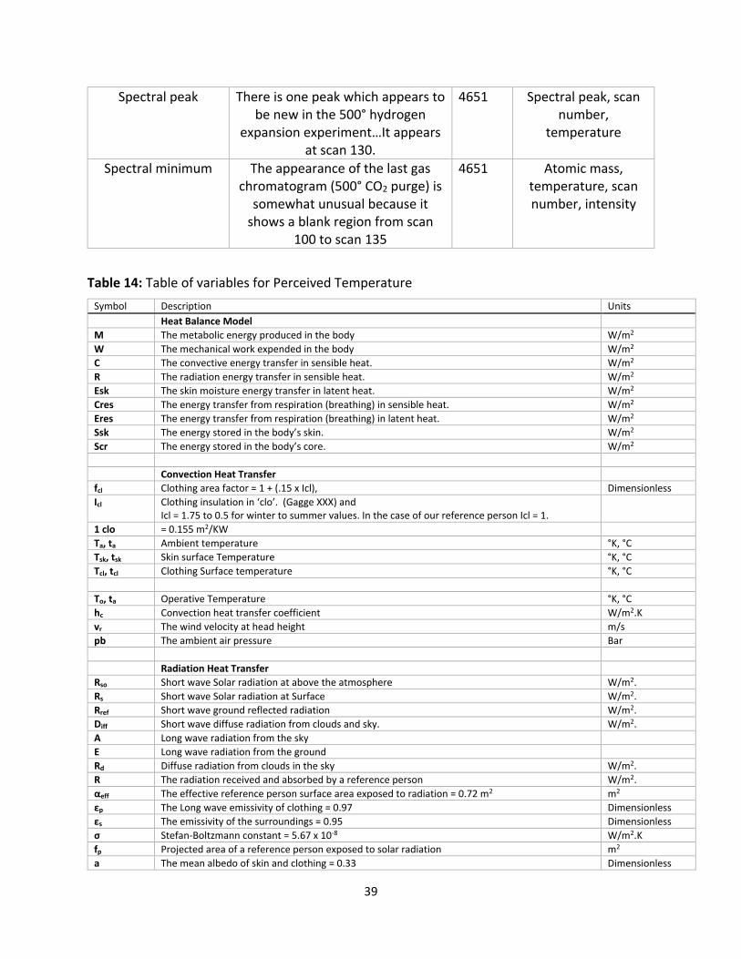
39
Spectral peak There is one peak which appears to be new in the 500° hydrogen
expansion experiment…It appears at scan 130.
4651 Spectral peak, scan number,
temperature
Spectral minimum The appearance of the last gas chromatogram (500° CO2 purge) is
somewhat unusual because it shows a blank region from scan
100 to scan 135
4651 Atomic mass, temperature, scan number, intensity
Table 14: Table of variables for Perceived Temperature
Symbol Description Units
Heat Balance Model
M The metabolic energy produced in the body W/m2
W The mechanical work expended in the body W/m2
C The convective energy transfer in sensible heat. W/m2
R The radiation energy transfer in sensible heat. W/m2
Esk The skin moisture energy transfer in latent heat. W/m2
Cres The energy transfer from respiration (breathing) in sensible heat. W/m2
Eres The energy transfer from respiration (breathing) in latent heat. W/m2
Ssk The energy stored in the body’s skin. W/m2
Scr The energy stored in the body’s core. W/m2
Convection Heat Transfer
fcl Clothing area factor = 1 + (.15 x Icl), Dimensionless
Icl Clothing insulation in ‘clo’. (Gagge XXX) and Icl = 1.75 to 0.5 for winter to summer values. In the case of our reference person Icl = 1.
1 clo = 0.155 m2/KW
Ta, ta Ambient temperature °K, °C
Tsk, tsk Skin surface Temperature °K, °C
Tcl, tcl Clothing Surface temperature °K, °C
To, ta Operative Temperature °K, °C
hc Convection heat transfer coefficient W/m2.K
vr The wind velocity at head height m/s
pb The ambient air pressure Bar
Radiation Heat Transfer
Rso Short wave Solar radiation at above the atmosphere W/m2.
Rs Short wave Solar radiation at Surface W/m2.
Rref Short wave ground reflected radiation W/m2.
Diff Short wave diffuse radiation from clouds and sky. W/m2.
A Long wave radiation from the sky
E Long wave radiation from the ground
Rd Diffuse radiation from clouds in the sky W/m2.
R The radiation received and absorbed by a reference person W/m2.
αeff The effective reference person surface area exposed to radiation = 0.72 m2 m2
εp The Long wave emissivity of clothing = 0.97 Dimensionless
εs The emissivity of the surroundings = 0.95 Dimensionless
σ Stefan-Boltzmann constant = 5.67 x 10⁻⁸ W/m2.K
fp Projected area of a reference person exposed to solar radiation m2
a The mean albedo of skin and clothing = 0.33 Dimensionless
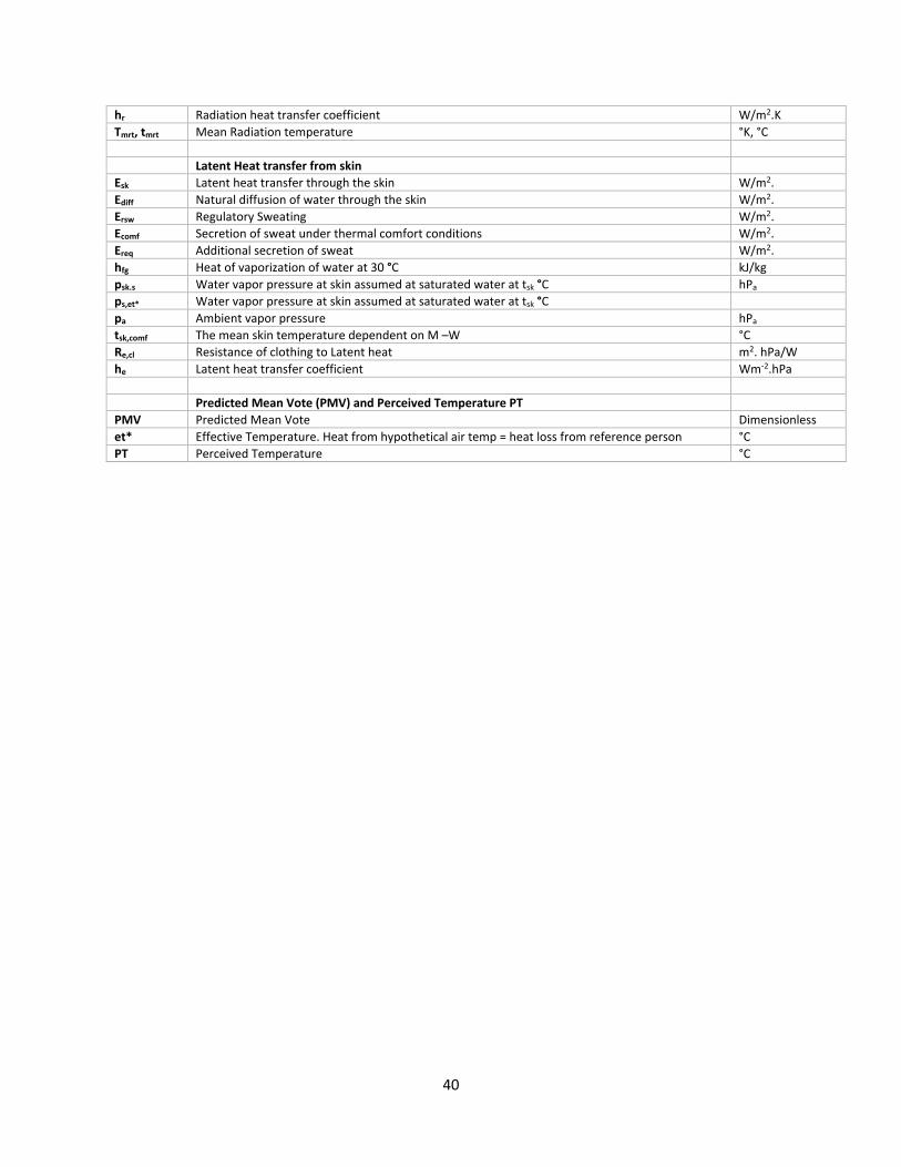
40
hr Radiation heat transfer coefficient W/m2.K
Tmrt, tmrt Mean Radiation temperature °K, °C
Latent Heat transfer from skin
Esk Latent heat transfer through the skin W/m2.
Ediff Natural diffusion of water through the skin W/m2.
Ersw Regulatory Sweating W/m2.
Ecomf Secretion of sweat under thermal comfort conditions W/m2.
Ereq Additional secretion of sweat W/m2.
hfg Heat of vaporization of water at 30 °C kJ/kg
psk.s Water vapor pressure at skin assumed at saturated water at tsk °C hPa
ps,et* Water vapor pressure at skin assumed at saturated water at tsk °C
pa Ambient vapor pressure hPa
tsk,comf The mean skin temperature dependent on M –W °C
Re,cl Resistance of clothing to Latent heat m2. hPa/W
he Latent heat transfer coefficient Wm-2.hPa
Predicted Mean Vote (PMV) and Perceived Temperature PT
PMV Predicted Mean Vote Dimensionless
et* Effective Temperature. Heat from hypothetical air temp = heat loss from reference person °C
PT Perceived Temperature °C