An Experimental Study of Acoustic Emission Methodology for in Service Condition Monitoring of Wind Turbine Blades

JialinTang1, 2, Slim Soua1, Cristinel Mares2, Tat-Hean Gan1, 2

1 Integrity Management Group, TWI Ltd, United Kingdom

2 College of Engineering, Design and Physical Sciences, Brunel University London, United Kingdom

Corresponding Author: Tel: +44 01223899527; Email: jialin.tang@affiliate.twi.co.uk (Jialin Tang)

Abstract

A laboratory study is reported of fatigue damage growth monitoring in a complete 45.7 m long wind turbine blade typically designed for a 2 MW generator. The main purpose of this study was to investigate the feasibility of in-service monitoring of the structural health of blades by acoustic emission (AE). Cyclic loading by compact resonant masses was performed to accurately simulate in-service load conditions and 187kcs of fatigue were performed over periods which totalled 21 days, during which AE monitoring was performed with a 4 sensor array. Before the final 8 days of fatigue testing a simulated rectangular defect of dimensions 1 m × 0.05 m × 0.01 m was introduced into the blade material. The growth of fatigue damage from this source defect was successfully detected from AE monitoring. The AE signals were correlated with the growth of delamination up to 0.3 m in length and channel cracking in the final two days of fatigue testing. A high detection threshold of 40 dB was employed to suppress AE noise generated by the fatigue loading, which was a realistic simulation of the noise that would be generated in service from wind impact and acoustic coupling to the tower and nacelle. In order to decrease the probability of false alarm, a threshold of 45 dB was selected for further data processing. The crack propagation related AE signals discovered by counting only received pulse signals (bursts) from 4 sensors whose arrival times lay within the maximum variation of travel times from the damage source to the different sensors in the array. Analysis of the relative arrival times at the sensors by triangulation method successfully determined the location of damage growth locations, which was confirmed by photographic evidence. In view of the small scale of the damage growth relative to the blade size that was successfully detected, the developed AE monitoring methodology shows excellent promise as an in-service blade integrity monitoring technique capable of providing early warnings of developing damage before it becomes too expensive to repair.

Keywords: Acoustic Emission, Fatigue, Structural health monitoring, Wind turbines Blade

1 Introduction

Wind energy is recognized as a reliable and affordable source of electricity in many countries. According to the Global Wind Report, by the end of 2014, the global wind energy capacity has reached 369.6 GW [1]. The wind turbine technology has advantages amongst other applications of renewable energy technologies due to its technological maturity, good infrastructure and relative cost competitiveness [2]. Success of a wind energy project relies on the reliability of a wind turbine system. Poor reliability will directly result in the increase operation and maintenance (O&M) cost and the decrease of the wind turbine system lifetime. To improve the wind turbine system reliability, it is important to identify critical components and characterize failure modes, this will allow the maintenance staff direct their monitoring, and focus on monitoring methods.

Wind turbines can suffer from moisture absorption, thermal stress, wind gusts and sometimes lightning strikes. Damage can occur at any part of the wind turbine, gear box bearings, generator bearing, wind turbines blades, a bolt shears, and a load-bearing brace buckles etc. [3]. As the blades are the key elements of a wind turbine system and the cost of the blades can account for 15–20% of the total cost, extensive attention has been given to the condition monitoring of blades [4]. Wind turbine blades’ most common used materials are carbon and glass fibre materials (GRP) [5] [6]. They can be damaged by rain, extreme wind, lightning, bird strikes, and UV rays [7]. Besides they are subject to the cyclic stress loading because they transfer the mechanical flow from the wind to the flow of up to several MW electricity powers. In service failure is thus a significant risk and can have catastrophic consequences, with detached blades able to fly free for up to a mile and high collateral damage to the tower and nacelle caused by out of balance torques [8]. It is usually difficult to predict

12

3

4

5

6

7

89

101112131415161718192021222324252627282930

31

323334353637383940

4142434445464748495051

the remained life time of a blade, but it is possible to determine the condition of the blade and warn of failure.

The application of condition monitoring has grown considerably in the last decade due to its ability to allow real time monitoring of assets as a means to achieve the goal of early failure detection [9]. The main wind turbine blade applicable condition monitoring techniques include strain measurements, ultrasonic testing and AE. For the wind-farm operator, using strain gages to record the load history in the wind turbine blade has the advantage of understanding loads caused by the damage which enables a better detection of potentially damaging situations. However, the operational conditions lead to a lack of robustness for the use of strain gages and this technique has not been widely used for condition monitoring. The application of fibre bragg grating (FBG) showed technical advantages over the conventional strain sensor [10] and it can be expected to become an important tool for condition monitoring in the near future. Ultrasonic testing for wind turbine has become an important tool due to its capability to provide information about the state of the composite materials beneath the surface such as exposing the dry glass fibre existence or delamination [11]. For this method, a high degree of operator skill and integrity is required, and the spurious indication could mislead unnecessary repairs.

Acoustic emission (AE) is elastic wave generated by a material when it undergoes inelastic strain or rupture. The crack initiation and propagation of cracks in composite has been successfully detected using AE [12][13][14]. One of the advantages of AE technique for wind turbine blade inspection is that it is a passive technique requiring no power input to the sensors. The sensors can be lightweight and readily embedded in a new blade or retrofitted to existing blades without any intrusive effects [15][16]. This of course offers the advantage of being applied into a condition monitoring system. However, a significant drawback of AE technique for crack growth monitoring in many applications is that there are many sources of AE other than the crack of interest. These sources thus constitute noise which can be both random and coherent, sometimes exceeding by far the crack signals. Such noise has been observed in operational conditions for wind turbine blades [17]. The steady wind impact will generate standing waves which will be largely time coherent but variable with the wind speeds; particularly gusts will generate time random components in the standing waves.

AE monitoring has been investigated on small-scale wind turbine blade tests under laboratory conditions. Joosse, P. A., et al. and Dutton, A. G., et al. [18] [19] showed it is able to detect the damage zones by the cumulative AE evens curve by a couple of sensors which locate along a 4.5 m long blade. The primary detecting method is based on Kaizer and Felicity Effect. Data were acquired during static tests and low frequency fatigue tests controlled under laboratory conditions, which lowered the difficulty of AE signal processing. Zhou, Bo et al. identified the fatigue cracks in a 3m long blade by using the fractal dimension (FD) analytical method [20]. This method quantitatively describes the non-linear fault features for identification and predicting the complex non-linear dynamic characteristics of AE signals. The complexity variations are linked with the energy changes in the AE signal by means of FD, providing a fast computational tool that tracks the existence of a crack. Niezrecki, Christopher, et al. focused on a 9m long blade fatigue testing, AE data was only recorded only when the loaded blade was in the top and bottom 10% of the peak deflection due to the flaw growth in a fatigue test occurs primarily near the maximum stress analysis. AE location calculations were conducted in real time, the AE events are defined as the arrival of a wave at three or more sensors within a time window which is calculated based on the wave velocity in the blade [21]. The results showed the located events near the crack correspond to a significant energy release. However, the in operation wind turbine blades experience various forms of loads and impact events, which can cause damage in any area at any time. Besides, wind turbines have more than quadrupled in size. The blade length today can be over 50 m. It is necessary to carry out the AE monitoring on a large wind turbine blade under a more complex, close to real in operation condition.

In this paper, a new technique for detecting AE crack growth signals from wind turbine blades in the presence of accurate simulation of the noise to be expected from the blade when in service is described. A fatigue damage growth monitoring test totalled 21 days in a complete 45.7 m long wind turbine blade was carried out, during which AE monitoring was applied continuously with a 4 sensor array. Before the final 8 days of fatigue testing a simulated rectangular defect of dimensions 1 m × 0.05 m × 0.01 m was introduced into the blade. The growth of delamination up to 0.3 m in length and channel cracking from this source was successfully detected from AE monitoring. By using the

5253

54555657585960616263646566

676869707172737475767778

7980818283848586878889909192939495969798

99100101102103104105

triangulation method, 29 AE event locations computed by triangulation are clustered around the induced defect providing evidence of the growth of damage originating from this source.

2 Experimental Rig

2.1. Wind Turbine Blade SupportThe blade under test was a glass-reinforced plastic composite blade, measuring circa 45.7 m in length, with 2 internal supporting webs running the entire length of the blade. An external view of the entire blade length is shown in Figure 1, prior to the tests. The blade was installed on the test stand with the suction side of the blade facing the test lab floor as shown in Figure 1 (b).

(a) Full length view of the blade prior to installation

(b) Close up view of the blade root on the test stand

Figure 1 Wind Turbine Blade under Test

1.

2.

2.1.

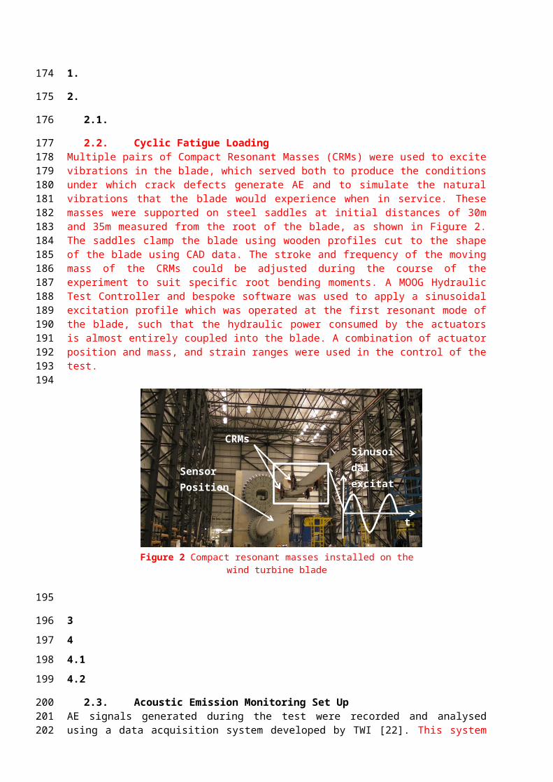
2.2. Cyclic Fatigue LoadingMultiple pairs of Compact Resonant Masses (CRMs) were used to excite vibrations in the blade, which served both to produce the conditions under which crack defects generate AE and to simulate the natural vibrations that the blade would experience when in service. These masses were supported on steel saddles at initial distances of 30m and 35m measured from the root of the blade, as shown in Figure 2. The saddles clamp the blade using wooden profiles cut to the shape of the blade using CAD data. The stroke and frequency of the moving mass of the CRMs could be adjusted during the course of the experiment to suit specific root bending moments. A MOOG Hydraulic Test Controller and bespoke software was used to apply a sinusoidal excitation profile which was operated at the first resonant mode of the blade, such that the hydraulic power consumed by the actuators is almost entirely coupled into the blade. A combination of actuator position and mass, and strain ranges were used in the control of the test.

Defect Location

106107

108

111112113114115

116117

118

119

120

121122123124125126127128129130131132133

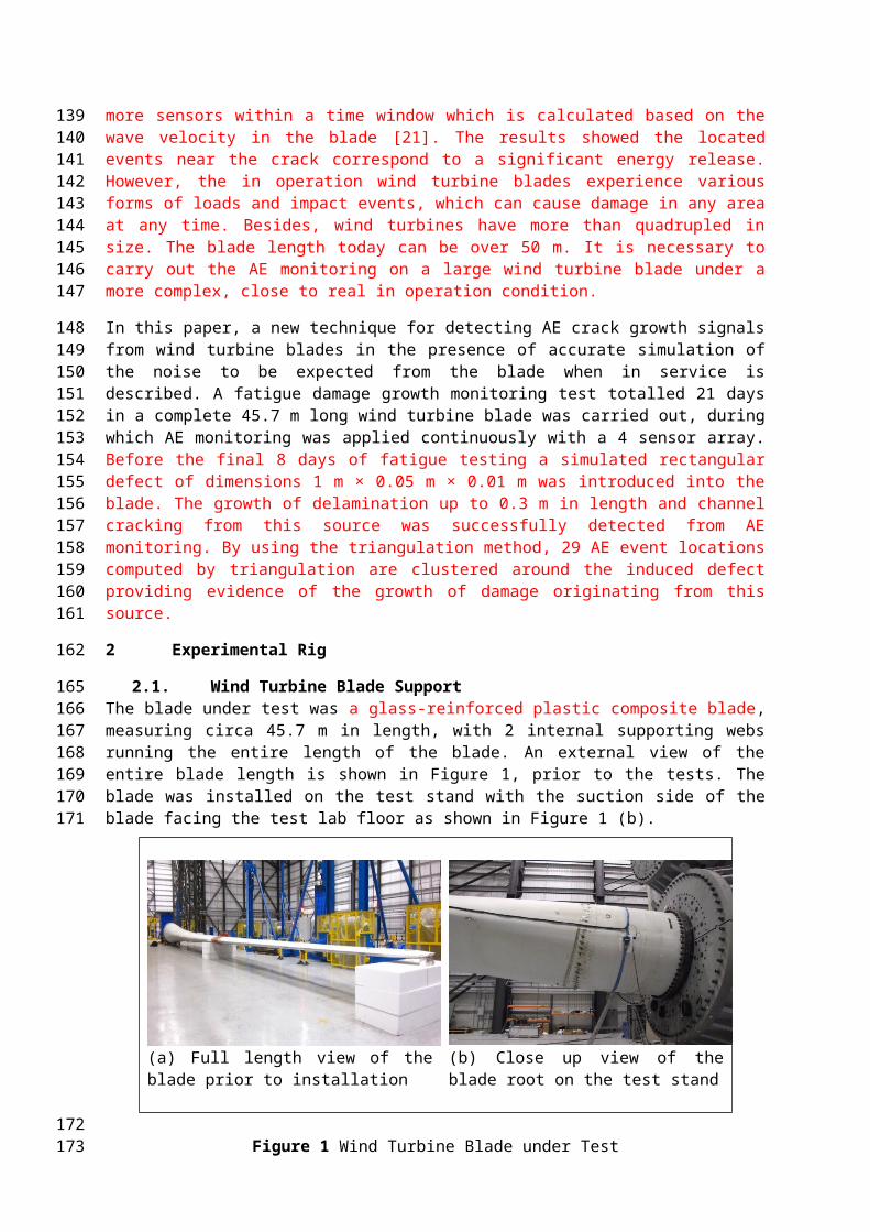
Figure 2 Compact resonant masses installed on the wind turbine blade

3

4

4.1

4.2

2.3. Acoustic Emission Monitoring Set UpAE signals generated during the test were recorded and analysed using a data acquisition system developed by TWI [22]. This system is based on the National Instruments PXIe-1071 card embedded in a bespoke enclosure which provide environmental and impact protection. The sampling rate was 500 kHz. A LabVIEW programme was used to control the data acquisition.

The wind turbine blade under test is large in size and wind turbine designers often employ an increased thickness section of GRP to increase strength. This creates challenges for AE monitoring in wave propagation because of wave attenuation. Attenuation will reduce the measured signal amplitude and this can cause lack of damage observability. By analysing the two primary wave modes which exist in the wind turbine blade, the extensional and flexural wave modes, Van Dam et.al [23] determined the dispersion curves, their results showing that the sensor spacing should be limited to a maximum value of 1m. In this study an attenuation test using pencil lead break was performed initially on the surface of the blade, in order to determine the required number and spacing of the sensors. Four sensors were used and the locations of the sensors are shown in Figure 3 and Table 1.

AE covers a wide frequency range (100 kHz – 1 MHz), classifications of failure modes in composites based on frequency content of AE signals have been investigated in [24] [25]. Three failure modes are identified with wavelet centred at: 300 kHz for fibre failure, 250 kHz for fibre-matrix debonding and 110 kHz for matrix cracking. As a result, four AE sensors with resonant 150 kHz frequency and having a good frequency response over the range of 100-550 kHz were used in the experiment. The sensors were connected to an external amplifier having a Gain of 34dB. The sensors are mounted on the blade internally in magnetic holders which engaged with steel collars adhesively bonded to the blade surfaces to ensure constant acoustic coupling, facilitated by the use of a gel couplant.

CRMs

Sensor Position

Sinusoidal excitation profile

t

134

135

136

137

138

139140141142143

144145146147148149150151152

153154155156157158159160

(a) AE sensors mounted between the two webs (b) AE sensors mounted the trailing edge side

Figure 3 AE sensors mounted internally on the blade.

Table 1 AE sensor locations

AE sensor number Location

AE1 In between webs, 9.8 m from rootAE2 In between webs, 8.2 m from rootAE3 Trailing edge side of web, 8.4 m from rootAE4 Trailing edge side of web, 9.6 m from root

3 Experimental Procedure

3.

3.1. Fatigue Testing

An evaluation of the vibration characteristics of the blade was carried out in a modal test prior to the fatigue test. The blade in service is most likely to be excited below the first natural frequency due to the observed frequency spectrum of the wind loads. Therefore the first natural frequency was selected as the frequency of cyclic loading during the fatigue test. The fatigue test equipment adding mass to the blade is shifting the natural frequencies of the system and the mode frequencies were determined as a function of the static mass loading when the CRMs were attached. A set of 5g accelerometers bonded to the surface of the blade at predefined locations allowed the response measurement during the modal test.

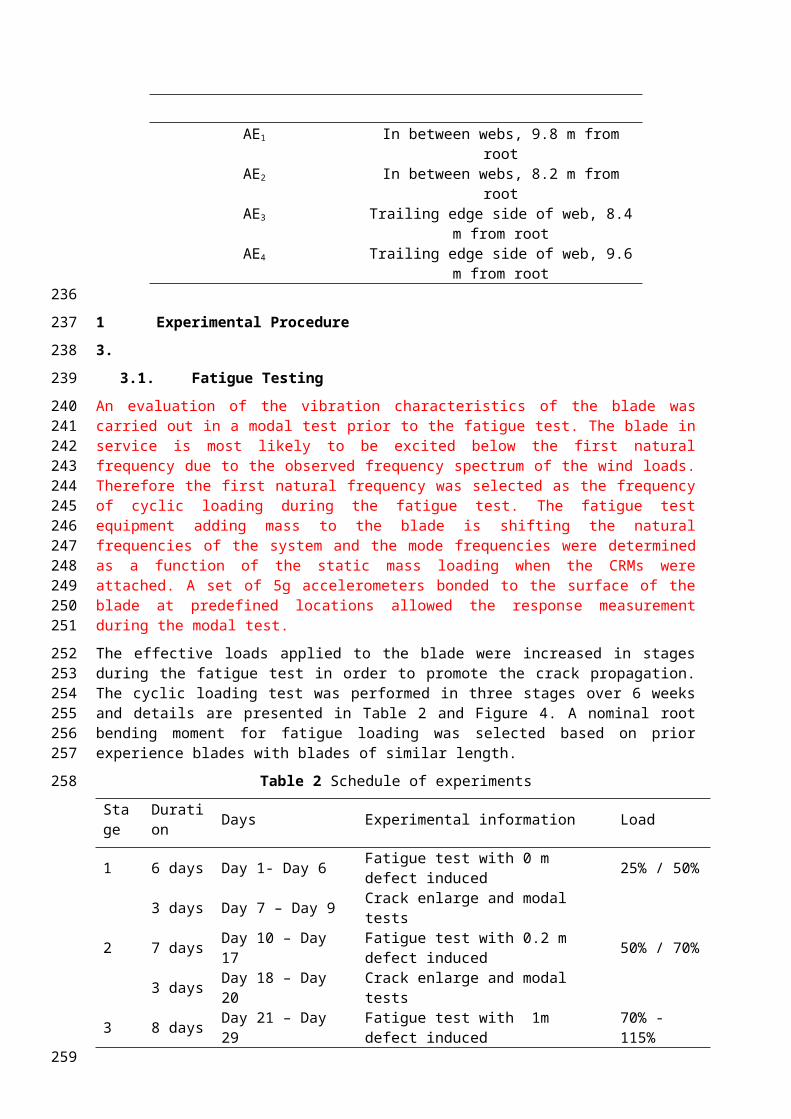
The effective loads applied to the blade were increased in stages during the fatigue test in order to promote the crack propagation. The cyclic loading test was performed in three stages over 6 weeks and details are presented in Table 2 and Figure 4. A nominal root bending moment for fatigue loading was selected based on prior experience blades with blades of similar length.

Table 2 Schedule of experiments

Stage Duration Days Experimental information Load

1 6 days Day 1- Day 6 Fatigue test with 0 m defect induced 25% / 50%3 days Day 7 – Day 9 Crack enlarge and modal tests

2 7 days Day 10 – Day 17 Fatigue test with 0.2 m defect induced 50% / 70%3 days Day 18 – Day 20 Crack enlarge and modal tests

3 8 days Day 21 – Day 29 Fatigue test with 1m defect induced 70% - 115%

161

162

163

164

165

166

167

168169170171172173174175

176177178179

180

181

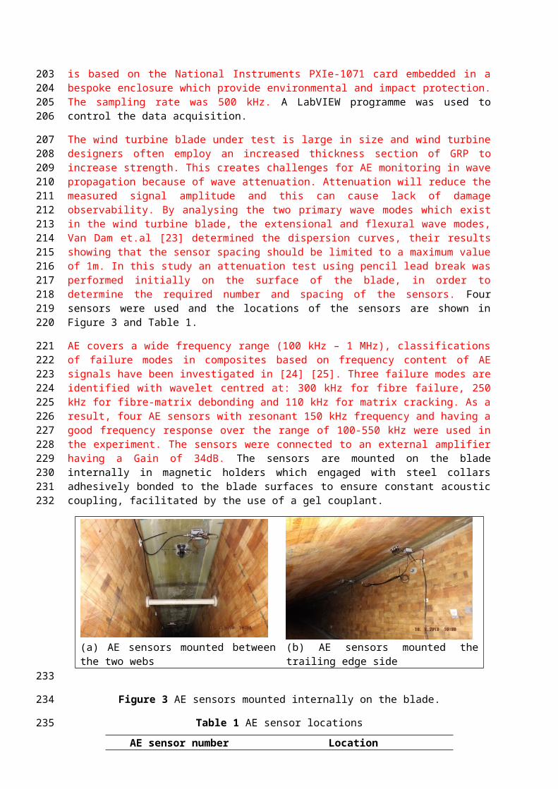
Figure 4 Nominal root bending moment of loading used versus number of cycles

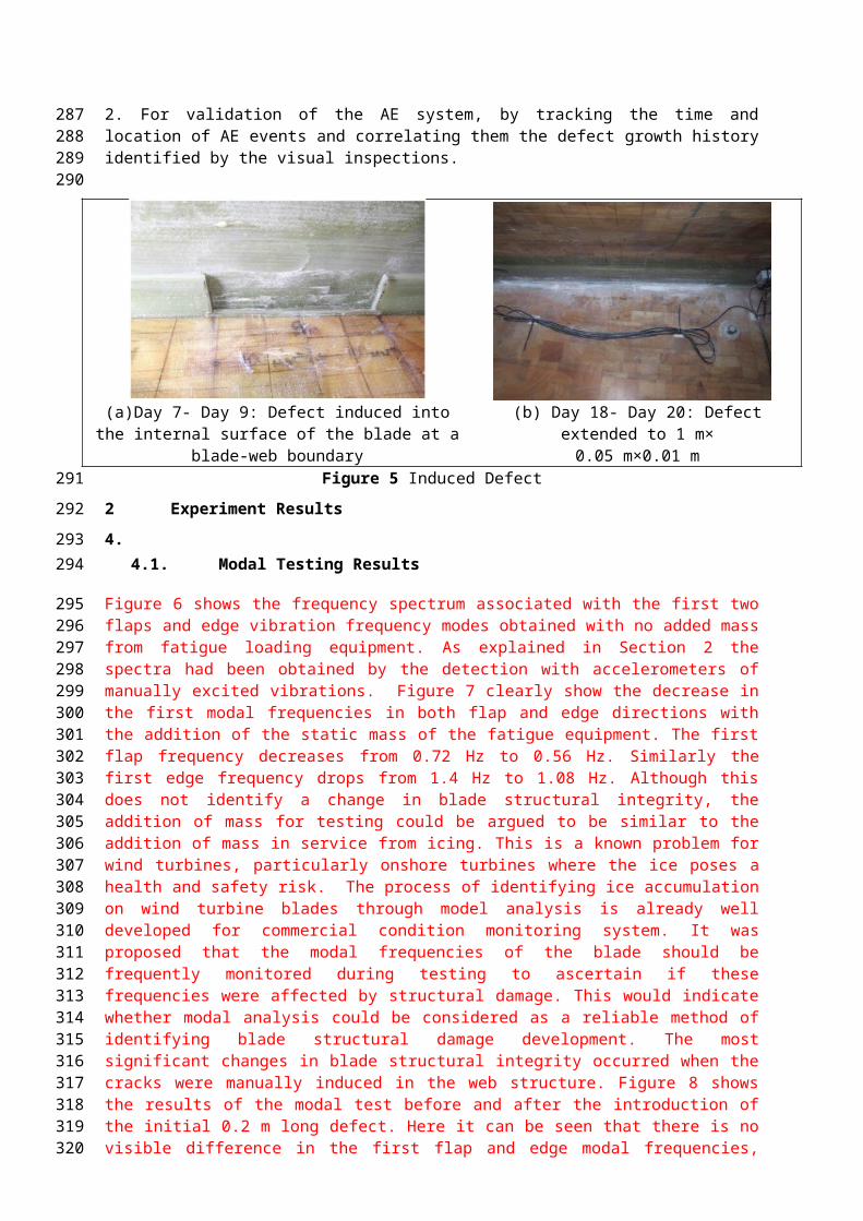
After roughly 67,000 fatigue cycles (Day 1- Day 6) at 50% nominal load, a 0.2 m (along the boundary)×0.05 m(perpendicular to the boundary) × 0.01 m(blade thickness direction) crack was made in one of the shear webs at 30m from the blade tip (Figure 5 (a)). The AE sensors were located in this region internally. Testing continued for a further 65,000 cycles (Day 10 – Day 17) at 50% and 70% load without any noticeable changes in the blade structure. It was then decided to increase the size of length of the induced defect to 1 m × 0.05 m × 0.01 m (Figure 5(b)) in order to increase the likelihood of further damage propagation for the purpose of evaluating the proposed AE damage monitoring technique. However, further testing at 70% load and then 80% yielded no noticeable change in the blade structure. So a decision was made to further increase the test load to 100% and subsequently this was increased further to 115% on the final day of testing.

3.

3.1.

3.2. Visual blade inspectionGenerally every second day throughout the tests the blade internal (at 9 m from the root) surfaces were inspected for crack initiation or propagation for two reasons:

1. To ensure that there was sufficient composite failure during the testing for verification of the AE system. 2. For validation of the AE system, by tracking the time and location of AE events and correlating them the defect growth history identified by the visual inspections.

0.2 m×0.05 m× 0.01 m defect introduction

1 m×0.05 m× 0.01 m defect introduction

Day 1 to Day 6 Day 10 to Day 17 Day 21 to Day 29

Nominal Bending Mo

Number of Cycles

182

183

184185186187188189190191192193

194

195

196197198199200201202203204

(a)Day 7- Day 9: Defect induced into the internal surface of the blade at a blade-web boundary

(b) Day 18- Day 20: Defect extended to 1 m×0.05 m×0.01 m

Figure 5 Induced Defect

4 Experiment Results

4.4.1. Modal Testing Results

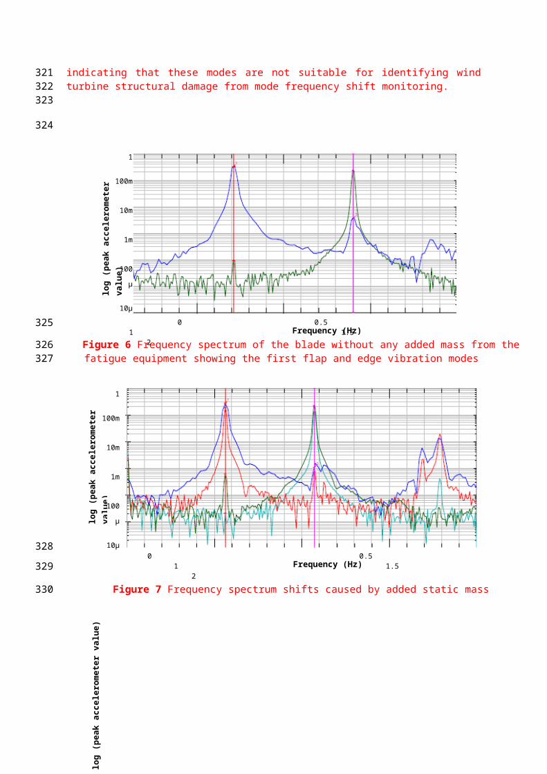
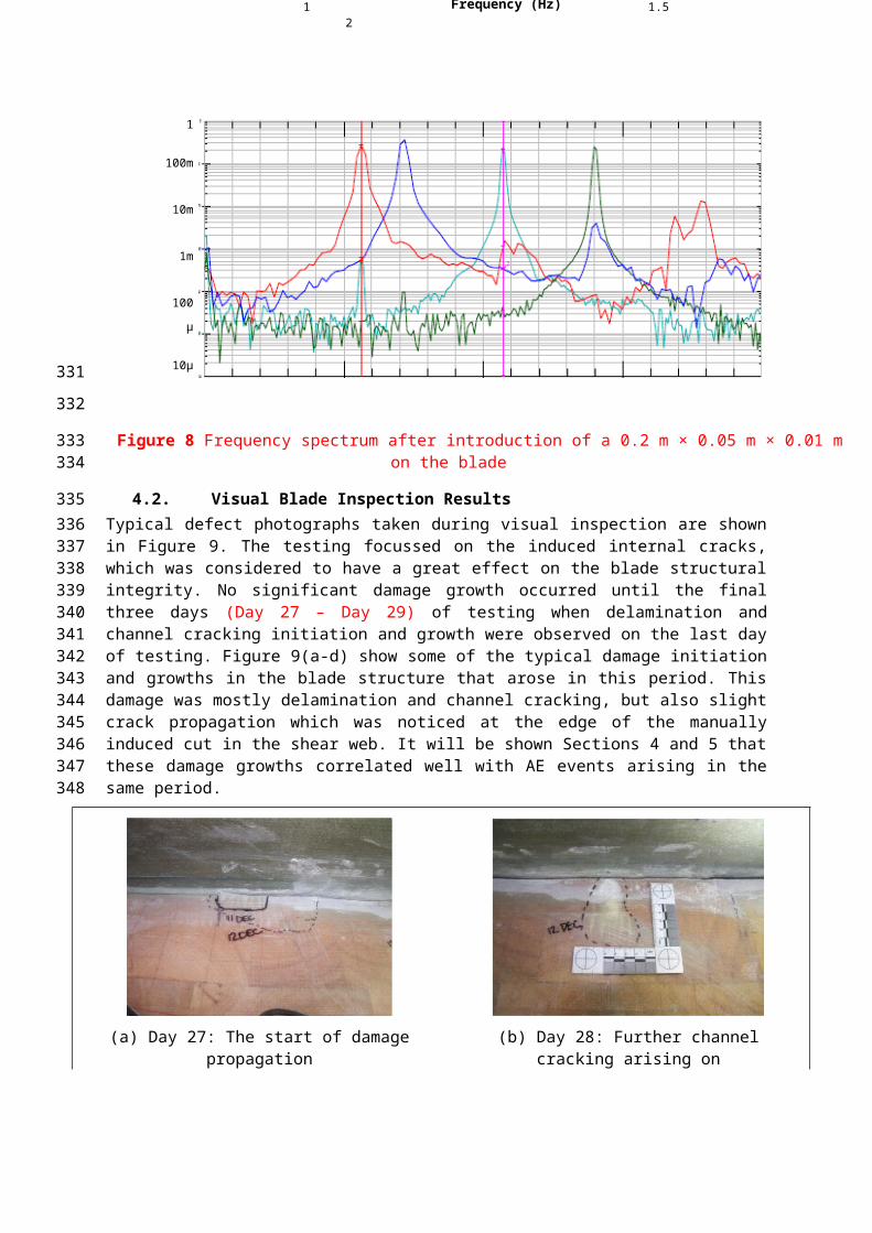
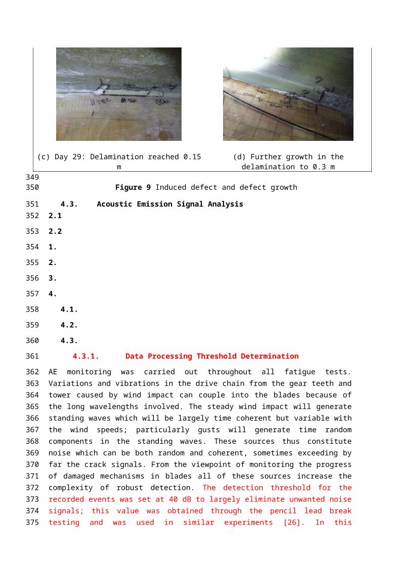
Figure 6 shows the frequency spectrum associated with the first two flaps and edge vibration frequency modes obtained with no added mass from fatigue loading equipment. As explained in Section 2 the spectra had been obtained by the detection with accelerometers of manually excited vibrations. Figure 7 clearly show the decrease in the first modal frequencies in both flap and edge directions with the addition of the static mass of the fatigue equipment. The first flap frequency decreases from 0.72 Hz to 0.56 Hz. Similarly the first edge frequency drops from 1.4 Hz to 1.08 Hz. Although this does not identify a change in blade structural integrity, the addition of mass for testing could be argued to be similar to the addition of mass in service from icing. This is a known problem for wind turbines, particularly onshore turbines where the ice poses a health and safety risk. The process of identifying ice accumulation on wind turbine blades through model analysis is already well developed for commercial condition monitoring system. It was proposed that the modal frequencies of the blade should be frequently monitored during testing to ascertain if these frequencies were affected by structural damage. This would indicate whether modal analysis could be considered as a reliable method of identifying blade structural damage development. The most significant changes in blade structural integrity occurred when the cracks were manually induced in the web structure. Figure 8 shows the results of the modal test before and after the introduction of the initial 0.2 m long defect. Here it can be seen that there is no visible difference in the first flap and edge modal frequencies, indicating that these modes are not suitable for identifying wind turbine structural damage from mode frequency shift monitoring.

Figure 6 Frequency spectrum of the blade without any added mass from the fatigue equipment showing the first flap and edge vibration modes

Frequency (Hz) 0 0.5 1 1.5 2

log

(pea

k ac

cele

rom

eter

val

ue)

1

100m

10m

1m

100 µ

10µ

1 µ

205

206

207208

209210211212213214215216217218219220221222223224225226227228

229

230

231232

Figure 7 Frequency spectrum shifts caused by added static mass

Figure 8 Frequency spectrum after introduction of a 0.2 m × 0.05 m × 0.01 m on the blade

4.2. Visual Blade Inspection ResultsTypical defect photographs taken during visual inspection are shown in Figure 9. The testing focussed on the induced internal cracks, which was considered to have a great effect on the blade structural integrity. No significant damage growth occurred until the final three days (Day 27 – Day 29) of testing when delamination and channel cracking initiation and growth were observed on the last day of testing. Figure 9(a-d) show some of the typical damage initiation and growths in the blade structure that arose in this period. This damage was mostly delamination and channel cracking, but also slight crack propagation which was noticed at the edge of the manually induced cut in the shear web. It will be shown Sections 4 and 5 that these damage growths correlated well with AE events arising in the same period.

Frequency (Hz) 0 0.5 1 1.5 2

1

100m

10m

1m

100 µ

10µ

1 µ

log

(pea

k ac

cele

rom

eter

val

ue)

1

100m

10m

1m

100 µ

10µ

1 µ

log (peak acceleromet

Frequency (Hz) 0 0.5 1 1.5 2

233

234

235

236

237

238

239240241242243244245246247248

(a) Day 27: The start of damage propagation (b) Day 28: Further channel cracking arising on

(c) Day 29: Delamination reached 0.15 m (d) Further growth in the delamination to 0.3 m

Figure 9 Induced defect and defect growth

4.3. Acoustic Emission Signal Analysis4.1

4.2

1.

2.

3.

4.

4.1.

4.2.

4.3.

4.3.1. Data Processing Threshold Determination

AE monitoring was carried out throughout all fatigue tests. Variations and vibrations in the drive chain from the gear teeth and tower caused by wind impact can couple into the blades because of the long wavelengths involved. The steady wind impact will generate standing waves which will be largely time coherent but variable with the wind speeds; particularly gusts will generate time random components in the standing waves. These sources thus constitute noise which can be both random and coherent, sometimes exceeding by far the crack signals. From the viewpoint of monitoring the progress of damaged mechanisms in blades all of these sources increase the complexity of robust detection. The detection threshold for the recorded events was set at 40 dB to largely eliminate unwanted noise signals; this value was obtained through the pencil lead break testing and was used in

249250

251252

253

254

255

256

257

258

259

260

261

262263264265266267268269270

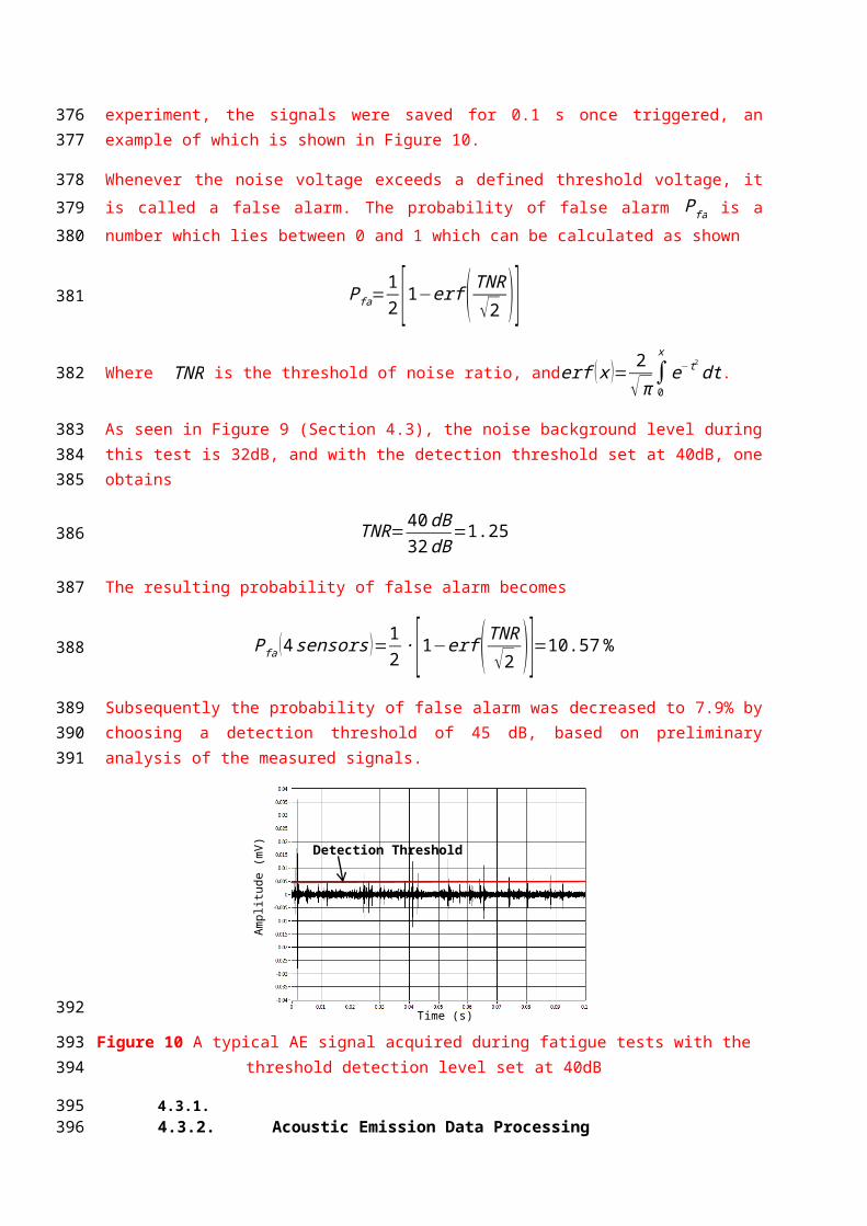
similar experiments [26]. In this experiment, the signals were saved for 0.1 s once triggered, an example of which is shown in Figure 10.

Whenever the noise voltage exceeds a defined threshold voltage, it is called a false alarm. The probability of false alarm Pfa is a number which lies between 0 and 1 which can be calculated as shown

Pfa=12 [1−erf (TNR

√2 )]Where TNR is the threshold of noise ratio, anderf ( x )= 2

√π∫0x

e−t2

dt .

As seen in Figure 9 (Section 4.3), the noise background level during this test is 32dB, and with the detection threshold set at 40dB, one obtains

TNR=40dB32dB

=1.25

The resulting probability of false alarm becomes

Pfa (4 sensors )=12 ∙[1−erf ( TNR

√2 )]=10.57 %

Subsequently the probability of false alarm was decreased to 7.9% by choosing a detection threshold of 45 dB, based on preliminary analysis of the measured signals.

Figure 10 A typical AE signal acquired during fatigue tests with the threshold detection level set at 40dB

4.3.1.4.3.2. Acoustic Emission Data Processing

Depending on the crack sources, AE signals can be roughly divided into three types, burst, continuous and mixed. Burst is a type of emission related to individual events occurring in a material that results in discrete acoustic emission signals. Continuous is a type of emission that related to time overlapping and/or successive emission events from one or several sources that results in sustained signals, it often comes from rubbing and friction. The mixed type signal contains both bursts and continuous and it is the type which is encountered in this test.

When a crack propagation incident occurs this is considered as an ‘AE event’. This event leads to a wave that can be recorded by different sensors with delays that depend on the distance between the

Detection Threshold (40dB)

Time (s)

Am

plitu

de (m

V)

271272

273274275

276

277

278279

280

281

282

283284

285

286

287288289290291292293294

295296

source and the sensors. Due to the visual crack growth prove, the signal analysis is based on the database acquired from day 21 to the end (after the 1 m × 0.05 m × 0.01 m crack was induced).

Initially in the monitoring programme all signals received by any sensor were recorded if they exceeded the threshold. The sum of all events within each day is simply equal to the number of measurements (data acquisition and processing operations) made in that day. Due to the coherent noise and vibrations, the initial data number set number was over 9000. AE data for this test was acquired without any restriction, thus there are five different situations concerning the acquired data:

1. None of the sensors acquired a burst, implying that the amplitude of all the signals acquired by all sensors is below the threshold.

2. Only one sensor acquired a burst.

3. Two sensors acquired a burst.

4. Three out of four sensors acquired a burst.

5. All four sensors acquired at least one burst.

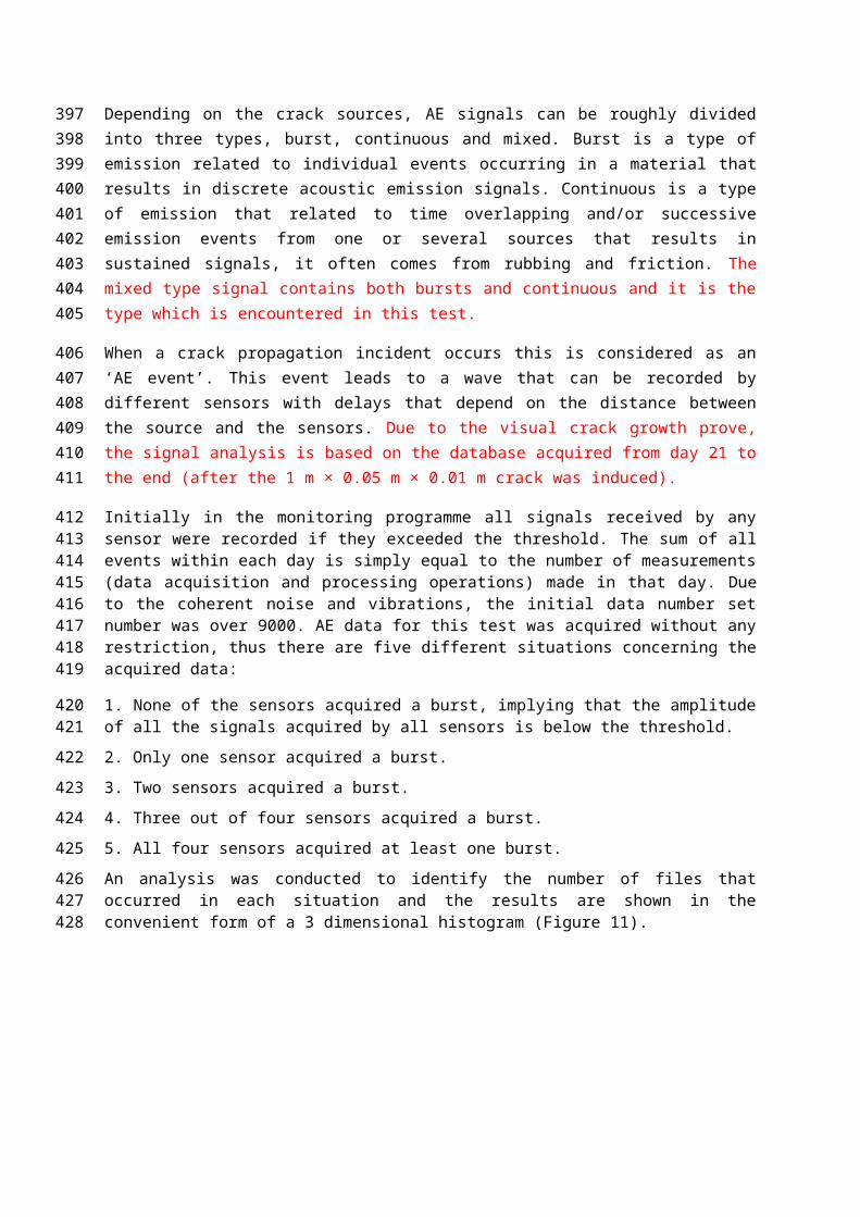
An analysis was conducted to identify the number of files that occurred in each situation and the results are shown in the convenient form of a 3 dimensional histogram (Figure 11).

Figure 11 Number of files in which bursts occurred in none, one, two, three or four sensors

After this step, the data processing focused on the 277 files which are the ones with all the four sensors acquired at least one burst at the processing threshold. And then, an AE event was defined as when all four sensors are hit within the time it would take for an AE signal to travel from its source through the shortest and longest distances to the four sensors, which was 150-500 µs. This value was calculated by dividing the shortest and longest distance from defect to senor by an average acoustic wave propagation velocity (2100 m/s) in the blade. Depending on the structure of the blade, the acoustic waves will travel in different waveforms and modes. The most common form of wave that travels in finite structure is the Lamb wave [28]. The wave velocity was determined through pencil lead break tests inside the blade [29]. There are 29 AE events left after this process.

297298

299300301302303

304305

306

307

308

309

310311

312

313

314315316317318319320321322323

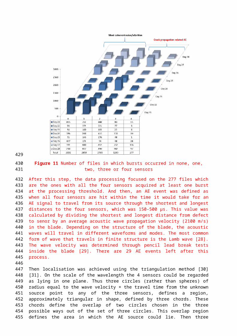
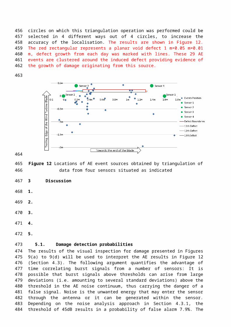
Then localisation was achieved using the triangulation method [30][31]. On the scale of the wavelength the 4 sensors could be regarded as lying in one plane. Thus three circles (rather than spheres) of radius equal to the wave velocity × the travel time from the unknown source point to any of the three sensors, defines a region, approximately triangular in shape, defined by three chords. These chords define the overlap of two circles chosen in the three possible ways out of the set of three circles. This overlap region defines the area in which the AE source could lie. Then three circles on which this triangulation operation was performed could be selected in 4 different ways out of 4 circles, to increase the accuracy of the localisation. The results are shown in Figure 12. The red rectangular represents a planar void defect 1 m×0.05 m×0.01 m, defect growth from each day was marked with lines. These 29 AE events are clustered around the induced defect providing evidence of the growth of damage originating from this source.

Figure 12 Locations of AE event sources obtained by triangulation of data from four sensors situated as indicated

5 Discussion

1.

2.

3.

4.

5.

5.1. Damage detection probabilities The results of the visual inspection for damage presented in Figures 9(a) to 9(d) will be used to interpret the AE results in Figure 12 (Section 4.3). The following argument quantifies the advantage of time correlating burst signals from a number of sensors: It is possible that burst signals above thresholds can arise from large deviations (i.e. amounting to several standard deviations) above the threshold in the AE noise continuum, thus carrying the danger of a false signal. Noise is the unwanted energy that may enter the sensor through the antenna or it can be generated within the sensor. Depending on the noise analysis approach in Section 4.3.1, the threshold of 45dB results in a probability of false alarm 7.9%. The probability that the signal will be detected is defined as probability of detection (POD),

POD=12 [1+erf ( SNR−TNR

√2 )]

mmmmmmmmm

m

m

m

m

m

324325326327328329330331332333334

335

336

337338

339

340

341

342

343

344

345346347348349350351352353354

355

─SNR is signal to noise ratio

For the calculation ofSNR, an average signal amplitude value is being used SNR=3.3. According to the above

POD=12 [1+erf ( SNR−TNR

√2 )]=97.1 %

This is a highly acceptable result, suitable for practical on line damage monitoring.

From inspection of Figure 10 (section 4.3) the following general conclusions can be reached:

1. There is no systematic trend over the entire fatigue cycle period for the data from sensors involving time correlated bursts from one and two sensors: high and low results are obtained in successive time slots throughout the entire cycle. So it is highly likely that these burst data are just spikes in noise continuum that exceed the threshold.

2. The time correlated bursts in 4 sensors do show a systematic trend. They are consistently low in successive daily intervals from day 21 to day 25. Then over day 26 to day 28, they increase very substantially and this coincides with the known onset of damage known from visual inspection, as illustrated in Figures 9 (a-d) (Section 4.2). Going back to the early data from day 21 to day 25, it is reasonable to infer from their consistency that they are damage signals rather than noise and that they indicate the early onset of damage which was too small to be evident in the visual inspections

5.2. Acoustic emission event locations: triangulationFrom inspection of Figure 12 (Section 4.3.2) it can be seen that the AE event locations computed by triangulation are clustered round 1 m×0.05 m×0.01 m void defect providing evidence of the growth of damage originating from this source. Quantitatively the 29 AE events locations have an average perpendicular distance from the defect axis of 0.6m ± 0.45m. 18 of these data (62%) have an average distance of 0.24m from this axis. In taking an AE pulse arrival time at any sensor as the first threshold crossing the most probable error in the arrival time measurement will be at least one wavelength, which as describe earlier is about 0.2m. This error exists because there is no ready means (especially given the slow rise time of the pulse envelope) of ensuring that the number N of the first cycle of the echo above threshold is the same with all events and all sensors.

Therefore it can be said that, within the experimental error in the AE threshold detection system, the 1m×0.05m×0.01m defect has been identified by AE monitoring as the source of growing fatigue damage.

3.

4.

5.

5.1.

5.2.

5.3. Prediction of the range of each sensor and the number of sensors required to achieve total volume coverage of a blade using AE

The average distance between the 4 sensors and the 29 damage locations is around 0.35 m. It is of interest to consider the number of distributed sensor required to provide complete coverage of a blade as the smaller is this number the more cost effective will be the monitoring system considered in terms of both capital and operational costs. The range of the AE signals is the key issue in this respect. Given the low frequencies of the signals, absorption of the signals by the blade material will not be the deciding factor. The amplitude attenuation α d cause by geometric factors will be the much more important. Even though the AE signals start out as spherical waves, α d will vary with the source-sensor distance d less rapidly than 1/d law because the wavelength is of the same order of magnitude

356

357358

359

360

361362363364365366367368369370371372

373374375376377378379380381382

383384385

386

387

388

389

390

391392393394395396397398399400

as the thickness of the blade wall and other structural members. After a number of sidewall reflections and mode conversions each initially spherically symmetric signal will become a mixed mode guided wave, approximating which will still be useful to monitor as an indicator damage growth. α d will be approximately a one dimensional function falling off as 1/√d.The amplitude signal to threshold ratio in the present experiments as indicated in Figure 9 (Section 4.3) is 5. A tolerable performance could be achieved is this ratio is reduced to 2, hence the available range for a sensor consistent with retaining the present performance is given by

0.35 ×1/√d=2 /5

Andd ≈ 0.8 m. Thus one sensor could monitor a range of 0.8 m in all directions so that for a 45 m long blade the number of sensors which could provide basic monitoring is

45 /(0.8 ×2)=28

Thus 28 sensors could provide basic monitoring and basic localization using trilateration could be achieved increasing three times the number of sensors. If the threshold could be reduced from 45 dB to 40 dB, thus accepting signal amplitudes reduced by a factor of 2, the signal to threshold ratio for the pulses shown in Figure 9 (Section 4.3) would be increased from 5 to 10. So, the range, given by0.35 ×1/√d=2 /10, would be increased to 3 m, reducing the sensor requirement for total blade coverage to a minimum of 8 sensors for basic monitoring and 32 for localisation. Such studies related to the robustness of localization test set up are very important for any experimental test.

6. Conclusion

1.

2.

3.

4.

5.

6.

6.1. Results summaryStarting from a simulated hole defect of 1 m × 0.05 m × 0.01 m dimensions in the GRP composite material of a 45.7m wind turbine blade the growth of real damage has been detected by continuous AE monitoring over 21 days of cyclic loading which simulated realistic loading conditions in service. Damage growth took the form of delamination, which grew to 0.3 m in length and also channel cracking, in the final two days of fatigue tests. The detection was achieved through correlations in the arrival times of burst signals from 4 sensors in the array. There is also evidence that the early stages of damage, too small to be detected visually, were detected by lower level AE events over the latest 8 days of fatigue testing after the introduction of the 1m long void defect. Only sets of bursts with arrival time separations equal to or less than the longest travel time difference for the bursts between the damage source and each sensor were accepted as a damage signal. When a similar acceptance procedure was applied for bursts from two sensors, or when bursts from all sensors were accepted, the damage signals could not be distinguished from noise peaks above the threshold setting. The detected damage is very small in extent compared with the size of the blade and thus small on the scale at which propagation to failure would be rapid. So the developed AE signal treatment technique employed, involving pulsed signal arrival time correlations, shows promise for on line blade monitoring. The threshold level for signal acceptance in the analysis was set at 45dB.

Using triangulation techniques applied to the relative arrival times of signals received by all 4 sensors damage growth locations were determined and found to be clustered round the defect. This was confirmed by the photographic evidence in Figure 9(a) to (d) (Section 4.2), although in addition, some

401402403404405406407

408

409410

411412

413414

415416417418419420421422

423

424

425

426

427

428

429

430431432433434435436437438439440441442443444445446447448449450

of the source localisations showed that the AE monitoring also detected damage too small to be detectable by visual inspection.

It was estimated that the number of sensors required for complete blade coverage was 28 for basic monitoring and 72 for damage localisation, using the 45dB threshold. However if the same AE performance could be achieved with a lower threshold of 40 dB (which will probably require additional signal processing for noise suppression) the number of sensors could be reduced to 8 for basic monitoring and 32 for damage localisation. However, these estimates need to be confirmed by experiment.

6.2. Future workIn Structural Health Monitoring, localisation and characterisation of damage represent two main stages of the process. For composite materials, the failure modes mainly include fibre breakage, fibre–matrix debonding and matrix cracking. In this paper the AE was used for localisation and characterization of the damage mechanisms on a wind turbine blade. The analysis was carried out in stages, the signals being filtered based on the information content above a noise threshold and in relation to the sensor test set up. Only signals which have enough energy to trigger all test sensors were considered for damage localisation, eliminating the signals that triggered only one or two sensors. This procedure produced a set of 277 events discriminated above the noise threshold from an initial set of 9000 measured signal data during the test. The results of the damage localisation method and the correlation with the induced damage evolution on the wind turbine blade are presented in a detailed manner. The developed AE monitoring methodology shows excellent promise as an in-service blade integrity monitoring technique capable of providing early warnings of developing damage.

References

[1] Global Wind Energy Council. Global Wind Report-Annual Market Update 2014. Report, Belgium, March 2014.

[2] Yang W X, Tian S W. Research on a power quality monitoring technique for individual wind turbines. Renewable Energy 2014; 75:187-198.

[3]Ashley F, Cipriano R J, Breckenridge S, Briggs G A, Gross L E, Hinkson J and Lewis P A. Bethany Wind Turbine Study Committee Report; 2007.

[4] Flemming M L and Troels S .New lightning qualification test procedure for large wind turbine blades Int. Conf. Lightning and Static Electricity (Blackpool, UK) 2003; 36:1-10.

[5] Zhou H F, Dou H Y, Qin L Z, Chen Y, Ni Y Q and Ko J M. A review of full-scale structural testing of wind turbine blades. Renewable and Sustainable Energy Reviews 2014; 33: 177-187.

[6] Brøndsted P, Lilholt H and Lystrup A. Composite materials for wind power turbine blades. Annual Review of Materials Research 2005; 35: 505–538.

[7] Galappaththi U I K, De Silva, A K M, Macdonald M and Adewale O R. Review of inspection and quality control techniques for composite wind turbine blades. Insight: Non-Destructive Testing and Condition Monitoring 2012; 54: 82–85.

[8] Robinson C M E, Paramasivam E S, Taylor E A, Morrison A J T and Sanderson E D. Study and development of a methodology for the estimation of the risk and harm to persons from wind turbines. Report, MMI Engineering Ltd, UK. 2013.

[9] Devriendt C, Magalhães F, Weijtjens W, Sitter G, Cunha Á and Guillaume P. Structural health monitoring of offshore wind turbines using automated operational modal analysis. Structural Health Monitoring 2014; 13(6): 644-659.

451452453454455456457458459

460461462463464465466467468469470471472473

474

475476

477478

479480

481482

483484

485486

487488489

490491492

493494495

[10] Arsenault, Tyler J., et al. "Development of a FBG based distributed strain sensor system for wind turbine structural health monitoring." Smart Materials and Structures 2013: 075027.

[11] Drewry, M. A., and G. A. Georgiou. "A review of NDT techniques for wind turbines." Insight-Non-Destructive Testing and Condition Monitoring 2007: 137-141.

[12] Christopher Baker, Gregory N. Morscher, Vijay V. Pujar, Joseph R. Lemanski, Transverse cracking in carbon fiber reinforced polymer composites: Modal acoustic emission and peak frequency analysis, Composites Science and Technology, 2015; 116: 26-32.

[13] Arumugam, V., Adhithya Plato Sidharth, A., Santulli, C. Characterization of failure modes in compression-after impact of glass–epoxy composite laminates using acoustic emission monitoring. Journal of the Brazilian Society of Mechanical Sciences and Engineering, 2015; 37 (5): 1445-1455.

[14] Stepanova, L.N., Chernova, V.V., Ramazanov, I.S.A procedure for locating acoustic-emission signals during static testing of carbon composite samples. Russian Journal of Nondestructive Testing, 2015; 51 (4): 227-235.

[15] Eaton, Mark, et al. "Use of macro fibre composite transducers as acoustic emission sensors." Remote sensing 1.2 2009: 68-79.

[16] Matt and Scalea [H.M. Matt, F.L. Scalea, Macro-fiber composite piezoelectric rosettes for acoustic source location in complex structures, Smart Mater. Struct. 16 (2007); 1489–1499.

[17] Vick B, Broneske S. ‘Effect of blade flutter and electrical loading on small wind turbine noise. Renewable Energy 2013; 50:1044-1052.

[18] Dutton, A. G., et al. "Acoustic emission monitoring from wind turbine blades undergoing static and fatigue testing." Insight 42.12 (2000): 805-8.

[19] Joosse, P. A., et al. "Acoustic emission monitoring of small wind turbine blades." Journal of solar energy engineering 2002: 446-454.

[20] Zhou, Bo, et al. "An Identification Method of Appearances and Expansion of Fatigue Crack in the Wind Turbine Blade Based on Fractal Feature."Advanced Materials Research. Vol. 591. Trans Tech Publications, 2012

[21] Niezrecki, Christopher, et al. "Inspection and monitoring of wind turbine blade-embedded wave defects during fatigue testing." Structural Health Monitoring (2014): 1475921714532995.

[22] Rafael S, Soua S, Zhao L, Gan T H, Makris N A and Kavatzikidis T. Guided waves focusing techniques for accurate defect detection in plate structures. Application of Contemporary Non-destructive testing in Engineering, PORTOROŽ, Slovenia, 4-6 September 2013.

[23] Van Dam, Jeremy, and Leonard J. Bond. "Acoustic emission monitoring of wind turbine blades." SPIE Smart Structures and Materials+ Nondestructive Evaluation and Health Monitoring. International Society for Optics and Photonics 2015.

[24] Ramirez-Jimenez, C.R., Papadakis, N., Reynolds, N., Gan, T.H., Purnell, P., Pharaoh, M. Identification of failure modes in glass/polypropylene composites by means of the primary frequency content of the acoustic emission event Composites Science and Technology 2004; 64 (12): 1819-1827.

[25] R. Gutkin, C.J. Green, S. Vangrattanachai, S.T. Pinho, P. Robinson, P.T. Curtis, On acoustic emission for failure investigation in CFRP: Pattern recognition and peak frequency analyses, Mechanical Systems and Signal Processing, 2011; 25: 1393-1407.

496497

498499

500501502

503504505506507508509

510511

512513

514515

516517

518519

520521522

523524

525526527

528529530

531532533

534535536

[26] M. Kharrat, E. Ramasso, V. Placet, M.L. Boubakar, A signal processing approach for enhanced Acoustic Emission data analysis in high activity systems: Application to organic matrix composites, Mechanical Systems and Signal Processing 2016; 70–71:1038-1055.

[27] Muravin, Boris. "Acoustic emission science and technology." Journal of Building and Infrastructure Engineering of the Israeli Association of Engineers and Architects, 2009.

[28] Lamb, Horace. "On waves in an elastic plate." Proceedings of the Royal Society of London. Series A, Containing papers of a mathematical and physical character 93.648 (1917): 114-128.

[29] Sause, Markus GR. "Investigation of pencil-lead breaks as acoustic emission sources." Journal of Acoustic Emission 2011; 29: 184-196.

[30] Manikas A, Kamil Y I and Willerton M. Source localization using sparse large aperture arrays. Signal Processing 2012; 60(12): 6617-6629.

[31] Kozick R J, Sadler B M. Source localization with distributed sensor arrays and partial spatial coherence. Signal Processing 2004; 52(3): 601-616.

537538539

540541

542543

544545

546547

548549