VIBRATION ANALYSIS OF A WIND TURBINE MULTI-STAGE …

VIBRATION ANALYSIS OF A WIND TURBINE MULTI-STAGE PLANETARY GEARBOX

INCORPORATING A FLEXIBLE BODY COMPONENT

A Thesis

presented to

the Faculty of California Polytechnic State University,

San Luis Obispo

In Partial Fulfillment

of the Requirements for the Degree

Master of Science in Mechanical Engineering

by

Tananant Boonya-ananta

December 2017

ii

© 2017


ALL RIGHTS RESERVED

iii

COMMITTEE MEMBERSHIP

TITLE: Vibration Analysis of a Wind Turbine Multi-Stage

Planetary Gearbox Incorporating a Flexible Body

Component

AUTHOR: Tananant Boonya-ananta

DATE SUBMITTED: December 2017

COMMITTEE CHAIR: Xi (Julia) Wu, Ph.D.

Professor of Mechanical Engineering

COMMITTEE MEMBER: Peter Schuster, Ph.D.


COMMITTEE MEMBER: Andrew Davol, Ph.D.


iv

ABSTRACT

Vibration Analysis of a Wind Turbine Multi-Stage Planetary Gearbox Incorporating a Flexible

Body Component


The following thesis document researches into creating a model to represent the behavior of a

wind turbine gearbox. This model is developed based on the overall parameters of a NORDEX

N90 2.5MW wind turbine developed by a German company Nordex SE. This research focuses

on the combination of a flexible body and a multibody dynamics analysis software. This is done

through the usage of MSC ADAMS, a multibody dynamic analysis program, and MSC

Patran/Nastran, a finite element analysis software, and its associated solver. The model is created

to show the vibration patterns of a healthy gearbox with rigid bodies, with a flexible body, and

with a defect applied on a particular gear in the planetary gear systems that is representative of

the N90 wind turbine. The flexible body incorporation allows for stress analysis of different gear

teeth at different locations.

Keywords: Gearbox, Nordex N90, Wind turbine, Fast Fourier Transform (FFT), Gear Mesh

Frequency (GMF), Planetary Gearbox, Vibration Pattern

v

ACKNOWLEDGMENTS

I like to extend my appreciation to Doug Malcolm from MSC Software Corporation who was

instrumental to the development of the working finite element model. I would like to also

express my gratitude to Dr. Wu for her guidance and advise as well as Dr. Schuster and Dr.

Davol for their input.

vi

TABLE OF CONTENTS

Page

LIST OF TABLES ....................................................................................................................... viii

LIST OF FIGURES ........................................................................................................................ x

CHAPTER 1. INTRODUCTION AND LITERATURE REVIEW ............................................... 1

1.1 INTRODUCTION ................................................................................................................. 1

1.2 LITERATURE REVIEW ...................................................................................................... 4

CHAPTER 2. – SYSTEM MODELING ........................................................................................ 7

2.1 SYSTEM MODELING – SOLIDWORKS COMPUTER AIDED DESIGN ....................... 7

CHAPTER 3. MSC PATRAN/NASTRAN FINITE ELEMENT MODEL ................................. 16

3.1 MODAL ANALYSIS/SUPERPOSITION .......................................................................... 16

3.2 PRELIMINARY MODAL ANALYSIS ............................................................................. 19

3.3 SOLIDOWORKS MODEL PREPARATIONS .................................................................. 21

3.4 MESH ANALYSIS ............................................................................................................. 23

3.5 STATIC ANALYSIS .......................................................................................................... 25

3.6 PATRAN FINITE ELEMENT MODEL ............................................................................ 26

CHAPTER 4. MSC ADAMS DYNAMIC MODEL .................................................................... 32

4.1 JOINTS AND CONSTRAINTS ......................................................................................... 32

4.2 CONTACT AND INTERATIONS ..................................................................................... 34

4.3 FORCE EXPONENT .......................................................................................................... 35

4.4 DAMPING .......................................................................................................................... 35

4.5 PENETRATION DEPTH ................................................................................................... 35

4.6 CONTACT STIFFNESS ..................................................................................................... 35

4.7 SYSTEM TORQUE ............................................................................................................ 37

4.8 SCALED MODEL .............................................................................................................. 39

4.9 SCALED MODEL MOTIVATION ................................................................................... 42

CHAPTER 5. DEFECT MODEL ................................................................................................. 46

5.1 CRACK/NOTCH MODEL DEFECT ................................................................................. 46

5.2 ADAMS VIEW FLEX ........................................................................................................ 50

CHAPTER 6. RESULTS .............................................................................................................. 54

6.1 GEAR RATIO VERIFICATION ........................................................................................ 54

6.2 STRESS ANALYSIS - STATIC ........................................................................................ 56

vii

6.3 STRESS ANALYSIS – DYNAMIC ................................................................................... 58

6.4 CONTACT FORCE ............................................................................................................ 65

6.5 FAST FOURIER TRANSFORM ....................................................................................... 67

6.6 VIBRATION ANALYSIS THROUGH FFT ...................................................................... 69

6.7 MULTISTAGE ANALYSIS............................................................................................... 74

6.8 VARYING INPUT SPEED VIBRATION TESTS ............................................................. 83

CHAPTER 7. CONCLUSION...................................................................................................... 98

REFERENCES ........................................................................................................................... 100

APPENDIX A - PATRAN TUTORIAL..................................................................................... 103

APPENDIX B - VIEW FLEX TUTORIAL ............................................................................... 137

viii

LIST OF TABLES

Page

Table 1. Gearbox components design parameters .....................................................................8

Table 2. Scaled model parameters ...........................................................................................14

Table 3. Mesh Convergence Study for Stress with Varying Seed Size ...................................24

Table 4. FEA model comparison with cantilever beam ...........................................................26

Table 5. Mesh Properties .........................................................................................................28

Table 6. Material Properties .....................................................................................................30

Table 7. Joint properties in Adams ..........................................................................................33

Table 8. Solid body contacts in Adams ...................................................................................34

Table 9. Torque and System Power .........................................................................................38

Table 10. Half Scale Solid Body Joints ...................................................................................41

Table 11. Calculated Component Velocities ...........................................................................54

Table 12. Static Analysis of a Sun Gear Tooth with varying defect size. ...............................57

Table 13. Stresses at six node locations of the gear tooth from the center to the face ............63

Table 14. FFT Stage 1 contact force between sun and planet gear frequency amplitudes ......70

Table 15. Comparison between amplitudes at the GMF harmonics of Stage 1 with and

without a defect at the sun gear tooth. .....................................................................72


without a defect at the sun gear tooth using flexible bodies. ..................................74





ix


without a defect at the sun gear tooth ......................................................................82

Table 20. Base Gear Mesh Frequencies for different speed input ...........................................83

x

LIST OF FIGURES

Page

Figure 1. Gear tooth involute profile .............................................................................................. 7

Figure 2. Gear tooth profile development in Solidworks ............................................................... 8

Figure 3. Gear tooth rotation to create full gear .............................................................................. 8

Figure 4. Full isometric Solidworks Assembly............................................................................. 12

Figure 5. Assembly exploded view ............................................................................................... 13

Figure 6. Scaled model assembly isometric .................................................................................. 14

Figure 7. First three bending modes for a beam with Fixed-Fixed boundary conditions [25] ..... 17

Figure 8. Simple beam with two constraint modes ....................................................................... 18

Figure 9. First vibration mode for the first stage sun gear ............................................................ 20

Figure 10. Eleventh vibration mode for the first stage sun gear ................................................... 20

Figure 11. Solidowrks model partitioned tooth ............................................................................ 21

Figure 12. Close-up of partitioned tooth ....................................................................................... 22

Figure 13. Meshed tooth for convergence study ........................................................................... 24

Figure 14. Convergence Study ...................................................................................................... 24

Figure 15. Patran geometry import model .................................................................................... 27

Figure 16. Patran close-up partition .............................................................................................. 27

Figure 17. Meshed Patran part ...................................................................................................... 29

Figure 18. Mesh close-up Patran .................................................................................................. 29

Figure 19. RBE2 Spider constraint of gear body .......................................................................... 31

Figure 20. Torque and System Power as a function of wind speed .............................................. 37

Figure 21. Full Assembly Half Scale Model – Solidworks Render .............................................. 39

Figure 22. Full Assembly Half Scaled Model - Adams ................................................................ 40

xi

Figure 23. Adams model with joint locations ............................................................................... 42

Figure 24. Gear stress contour plot ............................................................................................... 44

Figure 25. Configuration 1 - no defect.......................................................................................... 47

Figure 26. Configuration 2 - defect............................................................................................... 47

Figure 27. Notch radius mesh refinement at the sun gear of the first stage .................................. 48

Figure 28. Opposite side root mesh for compressive stress analysis ............................................ 48

Figure 29. Defect parameters dimensions ..................................................................................... 50

Figure 30. Adams Flex Control Module View ............................................................................. 52

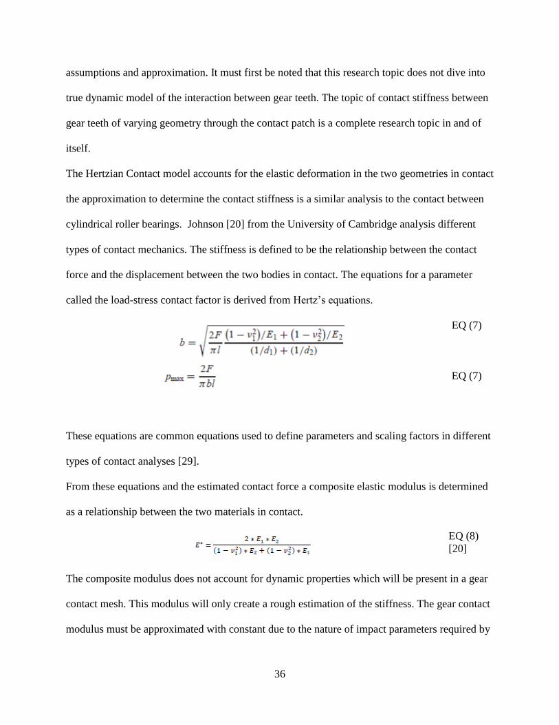
Figure 31. Stage 1 and Stage 2 Component Velocities ................................................................. 55

Figure 32. Three Stage velocities of all components .................................................................... 55

Figure 33. AISI 4820 Steel Estimated Non-Linear Stress vs. Strain Relationship ....................... 56

Figure 34. 25% Root Notch Deformed Body Front View ............................................................ 57

Figure 35. 25% Root Notch Deformed Body Notch View ........................................................... 58

Figure 36. Stress node probing in Adams ..................................................................................... 59

Figure 37. Stress node probe location 2 ........................................................................................ 60

Figure 38. Stress contour plot in Adams ....................................................................................... 61

Figure 39. Stress contour plot of finely meshed tooth in Adams.................................................. 62

Figure 40. Minimum principal, compressive, stress from the root center to the face .................. 63

Figure 41.Maximum principal, tensile, stress from the root center to the face ............................ 64

Figure 42. Maximum principal stress contour plo ........................................................................ 65

Figure 43. Minimum principal stress contour plot........................................................................ 65

Figure 44. Gear Contact Force Stage 1 Sun to Planets with Flexible Body. ................................ 66

Figure 45. Gear Contact Force Stage 1 Sun to Planets without Flexible Body. ........................... 67

xii

Figure 46. A signal viewed in frequency and time domain [23] .................................................. 68

Figure 47. Contact force FFT sun to planet Stage 1 ..................................................................... 70

Figure 48. Stage 1 contact force FFT between sun and planet gears with a defect on the sun gear

tooth. ............................................................................................................................................. 71

Figure 49. Stage 1 superposition comparison FFT of the contact force between the sun and planet

gear with and without a defect at the sun gear tooth. .................................................................... 72


gear with and without a defect at the sun gear tooth using flexible bodies. ................................. 73

Figure 51. FFT of Stage 1 contact force between sun and planet gear in a full three stage

assembly. ....................................................................................................................................... 75


assembly. ....................................................................................................................................... 76


assembly. ....................................................................................................................................... 76


assembly with a defect at first stage sun gear. .............................................................................. 77







xiii






assembly with input speed 1.5 rad/sec. ......................................................................................... 84


assembly with a defect at first stage sun gear with input speed 1.5 rad/sec. ................................ 84


gear with and without a defect at the sun gear tooth with input speed 1.5 rad/sec. ...................... 85







Figure 66. FFT of Stage 3 contact force between pinion and gear in a full three stage assembly

with input speed 1.5 rad/sec. ......................................................................................................... 88


with a defect at first stage sun gear with input speed 1.5 rad/sec. ................................................ 88

Figure 68. Stage 3 superposition comparison FFT of the contact force between the pinion and


xiv














with input speed 2.0 rad/sec. ......................................................................................................... 95


with a defect at first stage sun gear with input speed 2.0 rad/sec. ................................................ 96



1

CHAPTER 1. INTRODUCTION AND LITERATURE REVIEW

1.1 INTRODUCTION

Vibration analysis has been a core area of focus in the field of mechanical engineering for

decades. Vibrations exists in many varying scopes from vibrations of molecules to the vibration

of structures. The field of vibrations emphasizes on analyzing the frequencies at which objects

oscillate. A particular frequency at which vibrations revolves around is the natural frequencies of

a system, these are the frequencies at which an object tends to oscillate. Oscillation about an

undamped natural frequency is referred to as resonance, where the amplitude of oscillation can

be significantly greater than that of a periodic input frequency. The resulting effect of resonance

can cause catastrophic failures of structures or mechanisms.

In the analysis of rotating machinery, vibration patterns can be studied closely to determine

health of a particular system. In this case the gearbox of mechanical drive trains used to power a

vast variety of different mechanisms throughout the world also exhibits particular frequencies

which can be analyzed in order to determine the conditions of the gearbox without having to

fully disassemble the system. This is an advantageous method of monitoring the health of

machinery so as to be able to prevent critical failure of components which could very costly or

endanger lives.

There exists different vibration patterns for different types of components inside a gearbox.

These patterns can be created by the shaft, bearings, or, but not limited to, the gears themselves.

The gear meshes exhibit a vibration unique to the number of teeth between the meshing

components and the speeds at which they rotate. Wear and damage to gears will create a

different vibration pattern when compared to a baseline pattern. This output can be monitored in

2

order to protect the life of the gearbox and the mechanical system. A gear can be determined as

damaged and replaced before the damage propagates to the system as a whole.

A model of a gear system can be simulated in a program called MSC Adams which is identified

as a multibody dynamic analysis software. Adams allows for the creating of different types of

kinetic joints and body contacts for creation of a dynamic system. A dynamic model allows for

simulation of real world interactions which some other type of analyses may not offer. This

pertains to a finite element analysis (FEA). FEA is one of the most commonly used type of

system analysis in engineering. FEA is commonly used as a tool for analyzing boundary values.

A fundamental common type of analysis is a static analysis to determine the stress and

displacement profile of a geometry which would otherwise be difficult to compute with an

analytical model.

FEA and multibody analysis is often kept separate in each’s own respective area of expertise,

however the combination of these two methods of analyses would allow each to make up for

what the other program cannot perform. In the case of gear mesh analysis, a finite element model

(FEM) would allow for stress analysis at various locations throughout the gear body during

standard operating parameters. This indicates that stresses can captured under a dynamic force

condition and/or high speed applications, a situation in which FEA is able to capture but has

various limitations. MSC Adams has attempted to bridge the gap by incorporating Adams View

Flex and the Adams Durability Module. However, this add-on contains significant limitations as

to the level of complexity of a finite element model that can be created. View Flex is sufficient

for analyzing simple bodies but lacks the level of mesh refinement that which can be created for

more complex geometry.

3

Under the MSC family of programs MSC Patran/Nastran exists as a FEM creator and solver.

Nastran stands for NASA Structural Analysis; this program has existed since the mid 1900’s

originally created by NASA to aid in increasing the efficiency of aerospace vehicles. Nastran

acts as the solver for FEM inputs. The current pre-mesher or meshing software that is directly

compatible and integrated with Nastran is MSC Patran. Patran/Nastran currently rivals popular

FEA software such as Abaqus CAE and ANSYS. The advantage of Patran/Nastran is also its

compatibility with Adams, with both programs being owned under MSC. Patran/Nastran allows

the generation of files that is easily interfaced with Adams models to combine the two family of

engineering analysis fields, finite element analysis and multibody dynamic analysis. Other rival

FEA software also have similar capabilities, however there are much more complicated

procedures which are required to allow the integration.

This thesis project investigates the effect and advantage of a flexible body into a multibody

dynamic analysis of a wind turbine gearbox. The vibration pattern of the planetary gear system is

analyzed through Adams to distinguish certain properties that develop due to a crack or defect on

a particular gear in the system. A flexible body representation of a sun gear in the planetary gear

system can be analyzed for the stresses at the root of a specific gear teeth with or without defects.

This type of analysis can help diagnose gearbox health and prevent critical failure and damage to

a larger system as a result of one component. This research combines a FEA and multibody

dynamic analysis using MSC Adams and Patran/Nastran and analyzes the vibration pattern

through multiple stages of a planetary gear systems. With the help of previous research and the

development of the design for a particular gearbox that models the parameters of a N90 wind

turbine developed by Nordex SE in Germany, this research can be done to develop a model

which has a significant and direct application.

4

1.2 LITERATURE REVIEW

The area of study involving gear mesh systems is a very involved field and has been studied for

many years. Planetary gearboxes are used in a wide variety of applications as the mode of power

transfer. In this particular case, Nordex uses a two-stage planetary and single stage fixed axis

gearbox to power the N90 2.5MW wind turbine [1]. Wind energy is one of the fastest growing

renewable energy industry in the world [2]. Aitken outlines that wind energy is expected to reach

a goal of providing 12% of the world’s electricity requirement in 2020 and 20% of Europe’s

energy demand [6]. However, with increasing operations, wind turbines continue to suffer from

component failure with high maintenance and repair costs as stated by the National Renewable

Energy Laboratories (NREL) in 2012 [3]. The NREL has continuously studied the efficiency on

methods to reducing or managing the high cost of drivetrain components in a wind turbine

gearbox of its 20-year life expectancy design. There have been many experimental test setups by

NREL to evaluate the effectiveness of the standard vibration analysis methodology.

The gear design process, outlined in Norton’s Design of Machinery [5], can be done to minimize

the frequency in which a single tooth can come in to contact with the other teeth on a meshing

gear. Multiple studies exist on analytical models of gear dynamics, Ozguven and Houser [9]

discuss the mathematical model of gear dynamics focusing on the theory and analytical methods

of representing gear mesh parameters. Puigcorbe and De-Beaumont discuss the high rate of

failure of gearbox design for wind applications arises from the inability to accurately predict the

loads, dynamic and static, which the system experiences at any given time [4]. This leads to high

engineering costs in design from over-engineering components to compensate for the high risk.

The field of study of monitoring wind turbine gearbox life has been an endeavor for a period of

time. Puigcorbe and De-Beaumont also point out a key feature of the standard design which has

5

yet to be resolved: the effect of improper rotor support inducing high loads to the structure and

gearbox [4]. The cost of maintaining such gear trains can quickly rise up to the $500,000 range.

Alemayehu and Ekwaro-Osire discuss the life expectancy of wind turbine gearboxes to range

from 3 to 7 years as opposed to the design expectancy of 20 years [8] in their study of the high

speed helical gear stage design. In a survey study conducted by Ribrant and Bertling [7] an

apparent trend has emerged that larger wind turbines have an increasing failure rate as opposed

to smaller turbines, which exhibits the opposite trend.

To attempt to combat this costly issue, Musial W., Butterfield S., and McNiff B [13] discuss the

attempt to improve wind turbine design by addressing three main points: possibility of

unaccounted loading, unpredictable non-linear load transfer and individual component reliability.

The resulting conclusion remains the same that new approaches to gearbox and system analysis

is require to address the failure issues at all levels of the design and manufacturing process.

Smolders et al. presents a reliable generic model representation of a wind turbine gearbox for

reliability predictions, including all critical components [10]. They conclude that the complexity

of a gearbox requires powerful analytical resources to more accurately predict the reliability.

More in-depth analysis of vibrational behavior has been performed on free vibration of planetary

gears by Lin and Parker [19] using a mathematical model defining natural frequency properties.

Using methods of Fast Fourier Transform, Wu, Meagher and Sommer performed research and

analysis on a differential planetary system introducing backlash and teeth damage [16]. This

analysis proves evident to detecting damaged components in a gear system through vibration

characteristics displayed on an FFT plot with varying amplitudes. With this analysis in mind,

incorporating a finite element model into a dynamic analysis will allow for stress evaluations on

the required feature of interest. This is can be done through the use of MSC Adams and

6

Patran/Nastran through methods of modal superposition [27]. A multibody dynamic analysis is

performed at California Polytechnic State University, by Bradaric, G. [17] on dynamic behavior

of a connecting rod through incorporating a flexible body into MSC Adams. This research

investigates the integration between a finite element modal and multibody dynamic analysis. A

conclusion was reached that the integrated systems can produce accurate stress for a dynamic

body. A similar analysis was performed using MSC Adams and Abaqus FEA software by

Sawatzky, Rene [11]. The focus of Sawatzky’s research was to design a model to create the

gearbox that would achieve the requirements of the Nordex N90 and analyze the first stage of the

planetary gear system. This paper will continue further analysis of the same N90 gearbox using

the combination of MSC Adams and MSC Patran/Nastran, but looking at the system as a whole

in all three stages.

7

CHAPTER 2. – SYSTEM MODELING

2.1 SYSTEM MODELING – SOLIDWORKS COMPUTER AIDED DESIGN

The system created using over all parameters provided through Nordex was modeled using the

combination of 3D Computer Aided Design (CAD) Software, Solidworks, and Matlab code. The

gear parameters are used to input to the Matlab code which generates a series of gear parameters

required to model the gear in CAD. These parameters include the dedendum, addendum, pitch

diameter, base diameter, and angle and direction of rotation for Solidworks. Along with these

values, a text file is generated with coordinates of an involute profile. Solidworks image quality

is turned to the maximum resolution and units are changed to metric. This involute profile is

imported into Solidworks to define the critical shape of the gear tooth.

Figure 1. Gear tooth involute profile

The involute profile is rotated about the center of the gear to the specified angle of rotation and

direction from the MatLab output file. The gear body and the gear tooth is extruded to thickness

and then patterned to the specific number of teeth.

8

Figure 2. Gear tooth profile development in Solidworks

Figure 3. Gear tooth rotation to create full gear

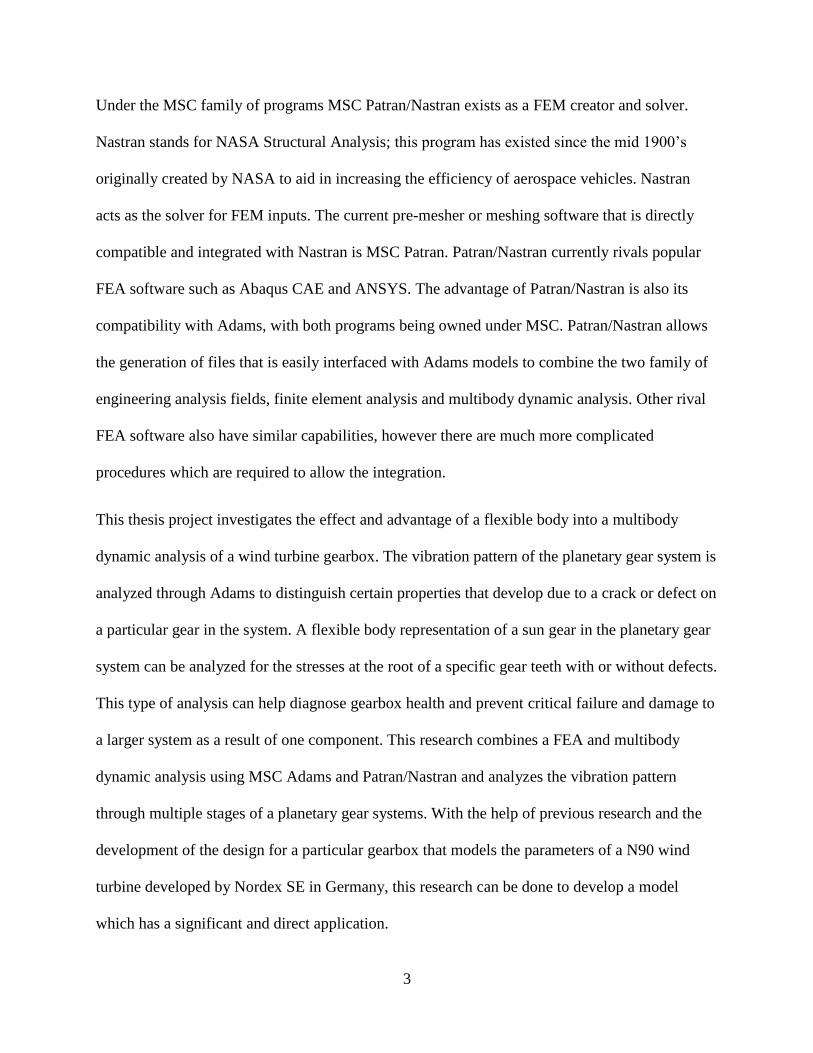
The gear parameters for all gears are shown in Table 1.

Table 1. Gearbox components design parameters

Part Teeth

Module

[mm]

Pitch

Diameter

[mm]

Model

Color

SolidWorks Part

9

Sta

ge

1 (

5.7

6 :

1)

Carrier

(Input)

- - -

Light

Blue

Planet 47 16 752 Blue

Ring 119 16 1904 Purple

Sun 25 16 400 Green

Sta

ge

2

Carrier

(Connected

to Sun 1)

- - - Green

10

Sag

e 2 (

11.0

6 :

1)

Planet 145 6 870 Yellow

Ring 322 6 1932 Dark Red

Sun 32 6 192 Red

Sta

ge

3:

(1.2

5 :

1)

Pinion

(Connected

to Sun 2)

40 6 240 Red

Gear

(Output)

32 6 192 Orange

11

Support - - - White

Table 1 defines full parameters for all three stages designed for the gear box. Each stage is

denoted with the associated gear ratio, number of planets, teeth on each gear, module, pitch

diameters, and a color indicator for the components. The parts are made with straight shafts

without any keyways or shoulders features for bearing location. This is done to simplify the

assembly for dynamic analysis in MSC ADAMS. The gear ratio is governed by the set overall

parameters of a minimum of 77.38 to 1 ratio, this ratio does not account for power losses and

represents the ratio between the input rotor speed and the generator input speed at maximum

power generation. A gear design criterion was created to determine the parameters for each gear

stage to achieve the necessary gear ratio as well as gears which are able to support loads

introduced into the system through the input torque. These loads seen throughout the system is

quite large thus resulting in gears which are non-standard size gears in the planetary system.

These gears range from about 200mm to 2000mm in diameter and each having a thickness of

150mm.

Through the gear design criteria, the gears determined for each stage were created with an

overall ratio of 5.76 to 1 in the Stage 1 (turbine side/input), 11.06 to 1 in Stage 2, and finally 1.25

to 1 in Stage 3. This results in an overall gear ratio of 79.6 to 1. The pitch angle used is a

standard angle at 20 degrees. With these parameters, each gear was modeled in SolidWorks

using the maximum modeling resolution combined with a script program written in Matlab. The

12

Matlab script is used to calculate pitch diameter, addendum, dedendum, base diameter and

rotation angle. The rotation angle incorporates the 1% backlash used to model the system. This

script provides a text file with coordinates for a tooth profile which is used in SolidWorks to

create the gear. The 1% backlash is incorporated with the involute profile is rotated and mirrored

to represent the tooth profile which is then extruded to a specified thickness then patterned. Stage

1 is designed to have gears with lower number of teeth which will see a larger input torque than

the other two stages, since as the gear speed increases in the system the torque decreases

proportionally with the gear ratio.

Figure 4. Full isometric Solidworks Assembly

13

Figure 5. Assembly exploded view

With the full scaled model in mind, another simplified model was created to scale down the

overall size on complexity which emanates for a full gear model with incorporated shafts. The

gear models were simplified using a scaling factor on the module of the gear. This effectively

causes the reduction of each gear model by the same factor as the reduction in the module. The

thickness of the overall gear can also be scaled down according to the desired factor. These

scaled models allowed for a much more efficient use of available computing resources for the

analysis.

The new scaled model is created with a module reduction of two. The effective gear properties is

reduced by the same factor. The thickness of the gear was chosen to be reduced by a factor of

five. The scaling factors created must be kept in mind when creating a force/torque input into the

system. The stress is ideally kept the same in order to represent the true behavior of the gear box

system. The new module specifications were input into the MatLab code and the properties were

generated input into Solidworks. The new model created, represents the basic gear model

without an incorporated shaft. The inclusion of a shaft running through the center gear body,

creates a significantly more complex model requiring more complex analysis with higher levels

14

of computing power. This will be further discussed in the theory of modal analysis and flexible

bodies. The system motion and constraint definitions are defined in ADAMS and will be

discussed in ADAMS system modeling. The new system model is shown in Figure 6.

Figure 6. Scaled model assembly isometric

Figure 6 shows the full system model of the three-stage assembly. This system is broken up into

three main parts; Stage 1, Stage 2, and Stage 3. Each of these stages are represented in the

Solidworks model with different configurations. These different configurations allow for model

to be imported into ADAMS for different types of analyses. Table 2 show the new parameter for

the models

Table 2. Scaled model parameters

Stage 1 Stage 2 Stage 3

Sun Plan Ring Sun Plan Ring Gear Pinion

Module 8 8 8 3 3 3 3 3

Thickness 30 30 30 30 30 30 30 30

Teeth 25 47 119 32 145 322 40 32

Pitch R 100 188 476 48 217.5 483 60 48

Adendum R 108 196 468.51 51 220 480.07 63 51

Dedendum R 90 178 486 44.25 213.75 486.75 56.25 44.25

Note: all relevant dimensions in millimeters

15

Table 2 indicates the new system model parameters and the associated parts color indicators.

Although, size reduction of the gears by reducing the model size through the module will not

affect computational load when the part is meshed in an FEA program, the thickness reduction

can effectively reduce the number elements.

16

CHAPTER 3. MSC PATRAN/NASTRAN FINITE ELEMENT MODEL

In order to introduce a flexible body analysis in to ADAMS, a modal analysis on the desired

body must be performed through the use of a finite element model (FEM). The FEM will be

generated with the same parasolid part file out of Solidworks into ADAMS. This is done to

ensure that the model remains in the same orientation and location when modeling in different

software. In this study, the FEM will be created using MSC Patran and MSC Nastran. Patran is a

FEM generator program which uses Nastran solver to run the analysis. A modal analysis on the

gear models can be performed in order to generate a flexible body for input into ADAMS for

dynamic analysis.

3.1 MODAL ANALYSIS/SUPERPOSITION

Modal superposition is the combination of linear, small deformation modes on a body. Through

this theory, a larger body can be defined as having different modes, deformation shapes, of

increasing order which are then superimposed. This allows for the representation of models with

a variety of degrees of freedom with a series of modal degrees of freedom. The overall vibration

characteristics of a body can be represented with the combined superposition of multiple mode

shapes. An example of three different mode shapes of a beam is represented in Figure 7.

17

Figure 7. First three bending modes for a beam with Fixed-Fixed boundary conditions [25]

The mode shape superposition approximation of the vibrational behavior of a model follows a

mathematical summation of the different mode shapes and their associated amplitudes.

𝑣(𝑥, 𝑡) = ∑ 𝜓𝑖(𝑥) ∗ 𝑞𝑖(𝑡)

𝑀

𝑖=1

Equation 1 shown is representative of the displacement of a body with respect to location, x, and

time, t, can be represented by the summation from the first mode to the Mth mode of the

corresponding mode shape, psi (ψ), scaled by q which is the amplitude of the vibration mode at a

specific time.

Since, normalizing the amplitude, q, ranging from 0 to 1, the mode shape can be analyzed at the

time which generates the maximum amplitude of each mode resulting in:

𝑣(𝑥) = ∑ 𝜓𝑖(𝑥) ∗ 𝑞𝑖

𝑀

𝑖=1

Equation (2) shows the deformation body depending on the sum of each consecutive mode shape

scaled but an amplitude factor, q, and position along the body, x.

EQ (2)

[26]

EQ (1)

[26]

18

The method of FEA incorporation into Adams is discussed in MSC Adams – Theory of Flexible

Bodies [27]. The original method utilized in Adams FEA was a method called the Guyan

reduction method. With this method the software, automatically reduces and condenses the

degrees of freedom (DOF) to reduce their number and computational intensity. This method

attempted to match natural frequencies and geometric properties using similar elements to those

created for the standard dynamic bodies. This produced undesirable results sometimes being

unable to match the total mass with the newly created lumped mass matrix.

The solution to the issues produced by earlier models of Adams Flex FEA modeling was the

development of the Craig-Bampton Method of Component Mode Synthesis (CMS). The CMS

method is an adaptation to Adams of the modern modal superposition theory. Within CMS,

specified DOF’s can be isolated from the modal superposition, this treats these nodes as

“boundary DOF” [27]. The static mode shapes are obtained by subjecting the boundary DOF to

“unit displacements while holding all other boundary DOF fixed” [27]. This generates the

constraint mode shapes, examples of these mode shapes are shown in Figure 8.

Figure 8. Simple beam with two constraint modes

Figure 8 shows two constraint modes for the left end of a beam with attachments at each end.

The left mode shape resembles a unit translation mode and the right a unit rotation mode.

To develop mode shapes suitable for dynamic analysis, the mode shapes are orthonormalized by

first solving for the eigenvectors to create a basis matrix following the relationship:

EQ (3)

[26]

19

The process of orthonomalizing creates a resulting set of mode shapes which are orthogonal

called Craig-Bampton modes [26], [27]. These modes are concluded to sufficiently address the

deficiencies of other models to represent a flexible body.

The integration between Patran/Nastran and ADAMS is created through a Modal Neutral File

(mnf). The mnf contains the information of the modal analysis performed by Nastran on the

FEM model from Patran. This file contains the flexible body with the associated properties

including but not limited to mass, geometry, element divisions, Young’s modulus, poisons ratio,

density and fixed node locations. The fix node locations act as fix point where the bearings

would generally be located, in the case on either ends of the gear shaft. The ability to

automatically generate a mnf is simplified through using Patran/Nastran for direct interface with

ADAMS to be analyzed using the Durability module, the programs are created by the same

software company under the name MSC and are made so that they can complement each other.

Other finite element software (FEA), such as Abaqus, are capable of generating a mnf as well,

however there are many features to that method which complicates the interface into ADAMS.

Due to the limitation of other FEA softwares. Patran/Nastran is used for this analysis. A

Patran/Adams Interface Tutorial document is attached as Appendix 1.

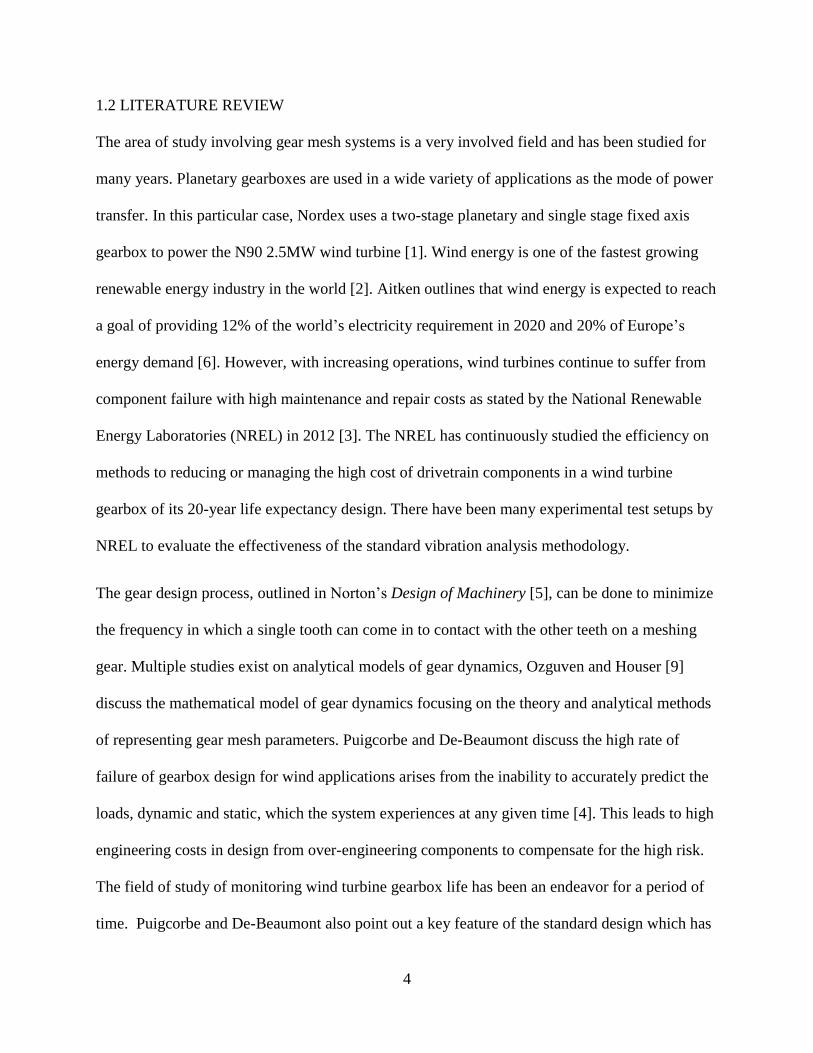
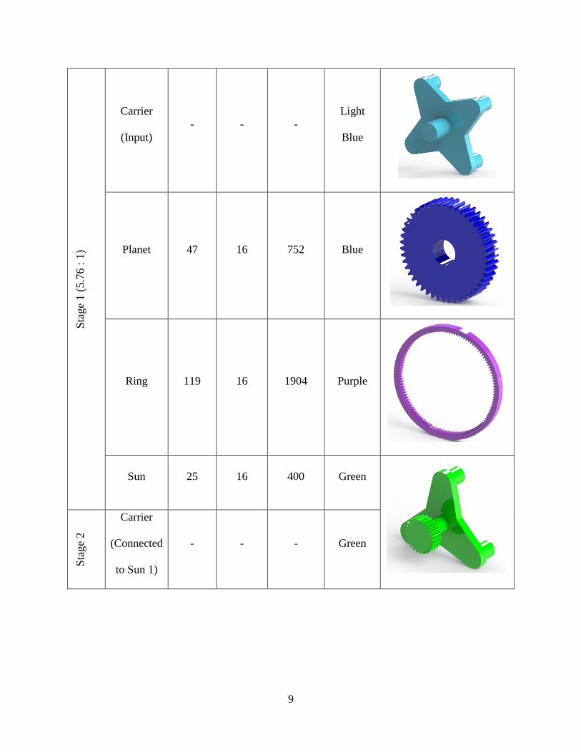
3.2 PRELIMINARY MODAL ANALYSIS

A modal analysis was performed on the sun gear to determine and create a visual representation

of the different modes the sun gear model undergoes. The modes seen in the modal analysis

simulate the modes that Patran/Nastran will use to create a combined modal for import to Adams

EQ (4)

[26]

20

to allow for a flexible body dynamic analysis. Figures 9 and 1 shows two of the

vibrational/deformation modes the model undergoes.

Figure 9. First vibration mode for the first stage sun gear

Figure 10. Eleventh vibration mode for the first stage sun gear

21

The series of modes seen in this analysis gives a general visualization of how the gear teeth

modes behave. Which allows for a better understanding of the theory behind the creation of a

modal analysis in Patran.

3.3 SOLIDOWORKS MODEL PREPARATIONS

The gear mesh under analysis is the fix axis gear mesh in Stage 3. The model developed for

mesh study is created in Solidworks with certain specific features so as to accommodate to

Patran when meshing the model to generate elements and nodes. A part model is shown in

Figure 11.

Figure 11. Solidowrks model partitioned tooth

22

Figure 12. Close-up of partitioned tooth

The split faced features developed in Solidworks in Figure 11 is done so that, in Patran, specific

seed sizes can be created on the body. A varying seed size is created to reduce the computational

load on the computer hardware. A fine mesh on the teeth and at the root will result in a fine mesh

on the entire part. This is very computationally intensive, generating result files from Patran that

are very large in size. A significantly more power computer is required in order to run a fine

mesh on the full part. The mesh seed creates a biased mesh with a fine mesh on the teeth and

teeth root and a courser mesh on the main body of the gear. This significantly reduces the

number of nodes and elements in the model which is directly related to the computational power

required to analyze the model.

By using Solidworks to split the faces on the model, this creates a prepartitioned part going in to

Patran and it also allows the selection of edges which would otherwise not be there in order to

create this varying mesh. To have a proper mesh for the desired location on the root of the tooth

in question to obtain accurate results, the partitions made allow for different element sizes at

different location.

23

3.4 MESH ANALYSIS

The mesh development process is done to ensure that the mesh is sufficient to provide a proper

representation of the stress at the required location. This results from the process of developing a

finite element analysis. When developing a representation of a solid model with the combination

of multiple elements, a minimum element size is required depending on the geometry of the

model in order to capture the full representation of the behavior of a body under a specified

loading condition. Each element is defined by a set of algebraic equations of a specified order,

generally either a linear or quadratic. An increase in the order of the element increases the

complexity of the model as well as the required computational resources. The underlying efforts

of a finite element model is to develop a model with a series of elements that is sufficient to

capture the behavior of the model for the specific analysis and no more. Over complicating a

finite element model is inefficient in terms of the resources required to perform a certain analysis

which is represented in computational time.

In order to determine the minimally sufficient element parameters to create the finite element

model, a mesh convergence analysis must be performed to show that the mesh does indeed

provide the necessary information to capture the required behavior of the model. Figure 13

shows the mesh analysis performed on a slice of a gear looking at the stress at the root of a single

tooth. These stresses for the required convergence of the mesh is depicted in Table 3 and Figures

13 and 14.

24

Figure 13. Meshed tooth for convergence study

Figure 14. Convergence Study

Table 3. Mesh Convergence Study for Stress with Varying Seed Size

Seed Size Fillet Stress

[mm] [MPa] %Change

1.00 277

250

270

290

310

330

350

370

0.00 0.20 0.40 0.60 0.80 1.00

Fille

t St

ress

[M

Pa]

Seed Size [mm]

25

0.50 333 20.19

0.25 362 8.60

0.125 361 0.18

Figure 13 shows the sufficient mesh created for an appropriate convergence to capture the stress

behavior on the root of the gear. Although, this test must be performed with measured values at

the desired location, an initial goal for the fine mesh at the desired location is to have at least 6

elements at the location of analysis [Source Doug MSC]. This general procedure must always be

verified, however it can be used as a starting point for defining element sizes.

A mesh convergence study will define a mesh that has converged once the stress variation is less

than 1% when reducing the element size by half. Table 3 shows the development of the mesh and

the changes in stress as the mesh refinement is increased by reducing element sizes. The

convergence study plot is shown in Figure 14 for root stress as a function of element seed size at

the specified location of interest. In Table 3 the change between 0.25mm edge seed sizes and

0.125mm shows slight variation of stress of 0.18%. The mesh can be defined as converged at

with this element size between 0.25mm and 0.125mm seed size, and 0.25mm seed size on this

model can be used. With a reduced model size, the same scale factor can be incorporated for the

mesh properties. The mesh convergence analysis is primarily significant to the location in which

the stress is to be analyzed. In this case the root stress of the gear in question.

3.5 STATIC ANALYSIS

To verify the appropriate range of stress for the validation of the finite element analysis, as static

cantilever beam analysis is performed to approximately predict the behavior of the stress at the

root of the tooth. This analysis is performed as a cantilever beam stress approximation

26

𝜎 =𝑀 ∗ 𝑦

𝐼

𝜎 =𝐹𝑡 ∗ 𝑟 ∗

ℎ2

112 ∗ 𝑏 ∗ ℎ3

EQ (5)

EQ (6)

In equation EQ(#), the variable Ft represents the tangential force applied to the gear. The variable

r represents the simulated moment arm. h represents the root thickness of the gear and b is the

face width of the gear.

Table 4. FEA model comparison with cantilever beam

Analysis

Stress

% Diff

[MPa]

Abaqus 362

28

Beam 282

A 30% difference as shown in Table 4 shows a respectable range for a beam representation of a

more complex geometry of the gear tooth. It must be noted that this stress calculation method is

quite simplified and is used to approximate the range at which the stress is expected to be. For

true estimates to gear bending stress and contact stress the AGMA standards must be applied.

3.6 PATRAN FINITE ELEMENT MODEL

The prepartitioned Solidworks model is imported into MSC Patran as a parasolid model. This

model is representative of the model to be used in ADAMS for dynamic analysis. This ensures

the proper orientation of the model when importing the .mnf file between programs. The part to

be created as a flexible body is isolated in Patran, this Stage 1 sun gear is shown in Figure 15.

27

Figure 15. Patran geometry import model

Figure 15 shows the tooth prepared for analysis inside of Patran. This is the same tooth in which

a defect will be later applied to compare final results after the dynamic multibody simulation

inside of ADAMS. A close up mesh location is shown in Figure 16.

Figure 16. Patran close-up partition

28

Figure 16 shows the primary location for the varying seed size assignments on the gear tooth.

The mesh parameters are show in Table 5 for each surface.

Table 5. Mesh Properties

Element Type

Element Shape

Function

Location

Seed Size

[mm]

Quadrilateral

(2 Dimensional)

Linear

(Quad4)

Root 0.125

Tooth Body 0.5

Gear Body 4

Thickness

Extrusion

5

The mesh is the symmetric for both sides of the gear tooth. The mesh created at the root for

stress evaluation is assigned as 0.125mm. This is in accordance with the mesh convergence study

performed for the same gear model at twice the size, thus a seed size of half of 0.25mm was

used. At the tooth and the surrounding area, a seed size of 0.5mm was used and the overall gear

was meshed using a 4.00mm seed size. The critical stress analysis point is concentrated at the

root of the gear tooth, and the relatively fine mesh is used for the tooth and the surrounding area.

The rest of the gear body and other teeth are meshed with a coarse mesh to reduce the number of

elements in the body for computational purposes. The gear tooth, itself does not require a mesh

as fine as that on the fillet at the root of the gear for accurate results. Figure 17 and Figure 18

shows the meshed gear body.

29

Figure 17. Meshed Patran part

Figure 18. Mesh close-up Patran

The mesh was created as a two-dimensional surface mesh on the face of the gear and then

extruded the thickness of the part. This method allows for a consistent mesh through the

30

thickness as opposed to meshing the whole solid instead with three dimensional elements which

produces undesirable results.

With a varying surface mesh on different areas of the gear face, there are nodes which are

created at the same locations on the same edge. These nodes will results in errors when

attempting to run the modal analysis. A process called ‘equivalence’ is used to eliminate these

nodes and associate the different meshes together along a common edge. Equivalence is

performed whenever a new mesh is created or elements are extruded next to other meshed

surfaces but still remain part of the original body. When the surface mesh is swept/extruded

through the thickness of the part with 5mm thick elements with 6 elements, Patran creates a

separate set of elements which are independent from the original solid. A material assignment

was created for each element and not the overall solid. The old solid is left as is without any

defined properties. Although the solid element has no defined properties, the analysis was still

performed on the remaining elements, this does not affect the solution; the undefined element is

remains un-“translated” by Patran/Nastran and can remain hidden. The material properties

entered into Patran are those represented in Table 6.

Table 6. Material Properties

Material AISI 4820 Steel / 18CrNiMo 7-6 / UNS G48200

Mass Density 7.77*10^-6 kg/mm3

Stiffness 210 GPa

Poison’s Ratio 0.29

Yield Strength 685 MPa

Ultimate Strength 840-1200 MPa

31

The constraint must be defined for the gear body so that the modal analysis can be performed.

The constraint location is positioned at the center of the gear body. A node is created to constrain

the internal face of the gear to the center of the geometry. The reference nodes created at the

center of the bore are connect with perfectly rigid body elements, this is defined in Patran as an

RBE2. The central node is defined with a set of degrees of freedom. The software uses this node

as the fixed boundary condition for analysis. This has a similar effect of defining a fixed

constraint (Abaqus) to the internal face of the gear, where all translational and rotation degrees of

freedom are constrained. Figure 19 illustrates this node relationship.

Figure 19. RBE2 Spider constraint of gear body

The RBE2 created is represented by the pink lines in Figure 19. These lines connect to each

internal node on the gear surface elements.

The normal mode analysis is performed by Nastran once Patran has completed its initial

translation of the elements. The modal analysis set up is created with 40 normal modes for the

gear body. Patran also includes 6 modes for the translation and rotation of the reference node

which creates a total of 46 modes of the model. This analysis generates the .mnf output file from

Nastran for input into ADAMS.

32

CHAPTER 4. MSC ADAMS DYNAMIC MODEL

Once the system is complete in Solidworks the file is converted to a parasolid for input into MSC

ADAMS, the file used is the same parasolid input for Patran. In ADAMS units are set

appropriately as millimeters, newton, kilograms and seconds (MMGS). The parasolid is then

imported into ADAMS.

.

The Adams assembly is located in the same place as where the origin is defined in the

Solidworks model. This assembly is representative of the full size system with incorporated gear

shafts and full gear bodies. The color identification of the parts remains the same from those

imposed in the Solidworks model once imported into ADAMS. This allows references back to

Table 1 for component parameters. Once assembly has been imported the density/material of

each part has to be defined. The martial properties for the material selected for the components

are defined in Table 6 under the finite element model section.

AISI 4820 Steel the mass density for Table 6 is enter for all components in the assembly. Note

the density must be defined in the specified working units, in this case material mass density is

converted to kg/mm^3.

4.1 JOINTS AND CONSTRAINTS

In reality, a wind turbine gear box will include the housing assembly, shaft splines, shaft

keys/keyways, as well as bearings in to locate the parts in the proper location. These additional

features will add higher order dynamics to the system due to bearing stiffness and rotor

imbalance due to non-symmetric geometry in the system. There are a variety of methods to

model, analyze or compensate for such system dynamics, however for the purposes of this

33

system, pure model is created with simple revolute joints connecting each part relative to each

other. The revolute joint for the full system is defined in Table 7.

Table 7. Joint properties in Adams

Stage Type Body 1 Body 2 Location

(Centered)

3

Lock Support Ground Ground

Revolute Input (gear) Support Ground

Output (pinion) Support Ground

2

Lock Ring 2 Ground Ground

Revolute

Carrier 2 Ring 2 Ring 2 center

Planet 2.1 Carrier 2 Carrier 2 Pin

axis


axis


axis

1


Revolute

Carrier 1 Sun 1 Ring 1 center


axis


axis


axis


axis

Revolute joint dynamics is simplified to a single rotational degree of freedom in a rigid joint.

This does now allow for any flexibility or compliance between the gears and the shaft in which

they are joined to. The location of the joints represent shaft and bearing location between the

gear body and its center shaft. Without bearing dynamics the gear only rotates about the central

axis of the shaft and has no out of plane movement. It is determined that under standard

operations, a uniform lateral load to the gear teeth throughout a cycle produces negligible out of

plane bending moments. Since the carrier shaft is realistically supported on both ends on either

side of the gear unlike the system model created, the load transfer to Stage 2 from Stage 1

34

through the carrier of the first stage driving the planets on the second stage also produces no out

of plane loads or bending moments.

Also seen in Table 7, the lock joints created between the ring gears and the final stage support.

The lock joint on the support is used to indicate a revolute joint for the Stage 3 fix axis gears

which would been realistically supported by the housing. The ring gear is designed to be fixed

with the chosen gear ratio between the stages.

4.2 CONTACT AND INTERATIONS

The interactions between the gear teeth is modeled in ADAMS as a contact force between each

body. The contact force represents the gear teeth mesh and must be created between each

meshing or contacting body in the system. The body contact forces are shown in Table 8.

Table 8. Solid body contacts in Adams

Body 1 Body 2

Stage 3 Output Pinion Sun 2

Stage 2

Sun 2

Planet 2.1

Planet 2.2

Planet 2.3

Ring 2

Planet 2.1

Planet 2.2

Planet 2.3

Stage 1

Sun 1

Planet 1.1

Planet 1.2

Planet 1.3

Planet 1.4

Ring 1

Planet 1.1

Planet 1.2

Planet 1.3

Planet 1.4

Table 8 shows the contact location between each meshing body in the system. These contact

forces are modeled as an Impact type contact. There are 4 different criteria that must be defined

for each contact stress: force exponent, damping, penetration depth, and contact stiffness.

35

4.3 FORCE EXPONENT

The force exponent, e, describe the elasticity of the contact. This represents the non-linear

function that models the impact contact parameter [15]. The value of e is a material property.

Stiffer material or hard metals such as steel will have an e value of approximately 2.2. For softer,

more malleable materials/metals as aluminum, e is approximately 1.5. For soft materials like

rubbers or certain polymers, e is approximately 1.1. It is recommended to that e > 1, a value less

than one can cause discontinuities during the impact.

4.4 DAMPING

The damping coefficient is determined to have a maximum value of 1% of the stiffness. This is a

non-physical property. Note that experienced individuals with this impact criteria believe that

1% is quite large and should be decreased. This general parameter is specified by MSC’s

characterization of contact impact modeling [21].

4.5 PENETRATION DEPTH

Penetration depth defines the behavior of the contact where damping varies between zero and the

maximum damping coefficient. This value has a positive relationship to the damping constant.

At lower penetration there is lower damping from zero until the maximum penetration which is

associated with maximum damping constant. The recommended penetration depth is generally

0.01mm

4.6 CONTACT STIFFNESS

Contact stiffness depends on the geometry of the contacting features, in this case the gear teeth

not just simply the material. The contact stiffness between the two gear faces can be modeled as

a Hertzian contact between two cylinders. The contact stiffness varies across the gear mesh as

the geometry/curvature of the face changes. The contact stiffness calculations require multiple

36

assumptions and approximation. It must first be noted that this research topic does not dive into

true dynamic model of the interaction between gear teeth. The topic of contact stiffness between

gear teeth of varying geometry through the contact patch is a complete research topic in and of

itself.

The Hertzian Contact model accounts for the elastic deformation in the two geometries in contact

the approximation to determine the contact stiffness is a similar analysis to the contact between

cylindrical roller bearings. Johnson [20] from the University of Cambridge analysis different

types of contact mechanics. The stiffness is defined to be the relationship between the contact

force and the displacement between the two bodies in contact. The equations for a parameter

called the load-stress contact factor is derived from Hertz’s equations.

EQ (7)

EQ (7)

These equations are common equations used to define parameters and scaling factors in different

types of contact analyses [29].

From these equations and the estimated contact force a composite elastic modulus is determined

as a relationship between the two materials in contact.

The composite modulus does not account for dynamic properties which will be present in a gear

contact mesh. This modulus will only create a rough estimation of the stiffness. The gear contact

modulus must be approximated with constant due to the nature of impact parameters required by

EQ (8)

[20]

37

Adams. The contact stiffness used for this simulation is used for the gear interaction is 5.0*106

N-mm [11].

4.7 SYSTEM TORQUE

At each stage of the assembly, there is an input and an output torque. The output torque will be

reciprocated into the stage as a resistive torque. The resistive torque is equivalent to the torque

seen in the system. The overall full system torque can be determined through from specifications

provided by the Nordex N90 data tables [1]. This torque representation is shown below in Figure

20 and Table 9.

Figure 20. Torque and System Power as a function of wind speed

0

200

400

600

800

1000

1200

1400

1600

0

500

1000

1500

2000

2500

3000

0 5 10 15 20

Torq

ue

[kN

m]

Po

wer

[kW

]

WindSpeed [m/sec]

pwr

TrqS1

TrqS2

TrqS3

38

Table 9. Torque and System Power

Wind Speed Power Speed S1 in S2 in S3in Out

m/s kW rad/sec kNm

0.0 0.0 0.0 0.00 0.00 0.00

0 0.0 0.0 0.0 0.00 0.00 0.00

3.5 27 1.76 15.3 2.71 0.24 0.20

4 73 1.76 41.5 7.32 0.66 0.53

4.5 129 1.76 73.3 12.93 1.17 0.94

5 197 1.76 112.0 19.75 1.79 1.43

5.5 277 1.76 157.4 27.77 2.51 2.01

6 371 1.76 210.9 37.19 3.36 2.69

6.5 480 1.76 272.8 48.12 4.35 3.48

7 608 1.76 345.6 60.95 5.51 4.41

7.5 754 1.76 428.6 75.59 6.83 5.47

8 916 1.76 520.7 91.83 8.30 6.64

8.5 1092 1.76 620.7 109.47 9.90 7.92

9 1279 1.76 727.0 128.22 11.59 9.27

9.5 1473 1.76 837.3 147.67 13.35 10.68

10 1671 1.76 949.8 167.52 15.15 12.12

10.5 1870 1.76 1062.9 187.47 16.95 13.56

11 2054 1.76 1167.5 205.91 18.62 14.89

11.5 2203 1.76 1252.2 220.85 19.97 15.97

12 2317 1.76 1317.0 232.28 21.00 16.80

12.5 2399 1.76 1363.6 240.50 21.74 17.40

13 2455 1.76 1395.4 246.11 22.25 17.80

13.5 2487 1.76 1413.6 249.32 22.54 18.03

14 2499 1.76 1420.5 250.52 22.65 18.12

14.5 2500 1.76 1421.0 250.62 22.66 18.13

15 2500 1.76 1421.0 250.62 22.66 18.13

15.5 2500 1.76 1421.0 250.62 22.66 18.13

16 2500 1.76 1421.0 250.62 22.66 18.13

16.5 2500 1.76 1421.0 250.62 22.66 18.13

17 2500 1.76 1421.0 250.62 22.66 18.13

17.5 2500 1.76 1421.0 250.62 22.66 18.13

18 2500 1.76 1421.0 250.62 22.66 18.13

The modeling methodology for input into the system includes two different approaches: a torque

input parameter or static angular velocity input. A static angular velocity input involves the

application of a motor element on a joint in Adams with accompanying resistive torque applied

39

to generate the contact force at each member of the assembly. Static motion input holds constant

angular velocity at the input. This angular velocity input is method in which this analysis has

been developed on. Although in certain cases, an input torque can be regarded as more realistic

as an input to the gear train, the input motion at steady state on the gear stages still remains

accurate to a wind turbine input parameter since the torque is represented through the system

stages.

4.8 SCALED MODEL

The scaled model is created for simplicity of simulation and computational time. The model

parts have a reduced gear module and thickness as well as a simplification of the connections in

the system. The modifications made to the gear assembly can be seen in Figure 21.

Figure 21. Full Assembly Half Scale Model – Solidworks Render

This model was imported to Adams in a similar method and definite of material. The Adams

model is shown in Figure 22. Some material was later removed to increase computational

efficiency.

40

Figure 22. Full Assembly Half Scaled Model - Adams

The simplified assembly is constructed with the same types of joints and constraints, however

there must be additional constraints added to relate each stage to the previous. The full joint set

up is show in Table 10.

41

Table 10. Half Scale Solid Body Joints

Stage Type Body 1 Body 2 Location

(Centered)

3 Lock

Support Ground Ground

Input (gear) Sun Stage 2 Sun Stage 2

center

Revolute Output (pinion) Support Ground

2

Lock

Ring 2 Ground Ground

Carrier 2 Sun Stage 1 Sun Stage 1

center

Revolute


axis


axis


axis

1


Revolute

Carrier 1 Sun 1 Ring 1 center


axis


axis


axis


axis

42

Figure 23. Adams model with joint locations

The elimination of the shafts on the model parts creates two different parts for the first stage sun

gear and the second stage carrier as well as the second stage sun gear and the third stage input

gear. In Table 10, it can be seen that a rigid joint is created in the method of a fixed joint to

constraint the revolution of the first stage sun gear to the second stage carrier and the second

stage carrier to the third stage input gear. The fix joint creates a ridged body constraint in

between the two bodies, this can be similarly represented with a rigid shaft.

4.9 SCALED MODEL MOTIVATION

The scaled model requires a modification of any resistive torque or torque input into the system.

The motivation for the scaled model is to reduce the effective computational time of the model

analysis but represent similar stress patterns in the process. The scaling method used to estimate

similar stress behavior is a static analysis of a cantilever beam similar to that performed to

estimate the range of the stress to be expected in the gear root. The governing equation for beam

bending stress is:

43

𝜎 =𝑀 ∗ 𝑦

𝐼

EQ (5)

The bending moment M in EQ(#), is representative of the tangential component of the contact

force between the meshing teeth. For a gear at half the module the moment arm is reduced by

half the original since the pitch radius is reduced by half. When analyzing for maximum stress y

is half the root thickness of the new gear tooth which is half the original thickness. The area

moment of inertia for a beam is represented by:

𝐼 =1

12∗ 𝑏 ∗ ℎ3

EQ (9)

The height of the beam is the root thickness of the tooth which is halved when the module is

halved. Finally, b represents the face width (gear body thickness). A relationship between the

original model and a new beam model can be made while keeping the bending stress constant:

𝐹𝑡1 ∗ 𝑟1 ∗ 𝑦1

112 ∗ 𝑏1 ℎ1

3=

𝐹𝑡2 ∗ 𝑟2 ∗ 𝑦2

112 ∗ 𝑏2 ℎ2

3

EQ (10)

Substituting in for the relationship between the two models yields:

𝐹𝑡1 ∗ 𝑟1 ∗ 𝑦1

112 ∗ 𝑏1 ℎ1

3=

𝐹𝑡2 ∗𝑟1

2 ∗𝑦1

21

12 ∗ 𝑏2 ∗ (ℎ1

2 )3

𝐹𝑡1 =2𝐹𝑡2 ∗ 𝑏1

𝑏2

EQ (11)

Converting the contact force into torque:

𝐹𝑡1𝑟𝑝1 = 𝑇1 𝑎𝑛𝑑 𝐹𝑡2𝑟𝑝2 = 𝑇2

2𝐹𝑡2 ∗ 𝑏1

𝑏2∗ 𝑟𝑝1 = 𝑇1

2𝑇2

𝑟𝑝2∗ 𝑏1

𝑏2∗ 𝑟𝑝1 = 𝑇1

44

2𝑇2𝑟𝑝1

2

∗ 𝑏1

𝑏2∗ 𝑟𝑝1 = 𝑇1

4𝑇2 (𝑏1

𝑏2) = 𝑇1

EQ (12)

The equation above shows an approximated torque scaling factor between a single fix axis gear

mesh with and an undefined face width scale factor.

The scaled modal also eliminates a portion of material at the center of the gear. An analysis was

performed on a slice of the gear body to determine the stress at the center of the gear as it

undergoes a static analysis from an applied simulated contact force. This analysis is show in

Figure 24.

Figure 24. Gear stress contour plot

Figure 24 shows the stress profile of a gear tooth from a portion of the gear due an applied force

at the contact patch. It can be seen that there is negligible or no deformation towards the center

45

of the gear body. This allows for the modeling of the gear body while neglecting the center

portion of the gear material.

46

CHAPTER 5. DEFECT MODEL

5.1 CRACK/NOTCH MODEL DEFECT

Different models are created in preparation for different stage analysis of the system. The sun

gear one the first stage is created with two different configurations; one representing a fully

healthy gear and the other with a defect at the root of the gear tooth. As a preliminary analysis of

this type of defect, the defect is created to extend approximately a quarter of the root thickness of

the gear. These two different configurations are shown in Figures 25 and 26

47

Figure 25. Configuration 1 - no defect

Figure 26. Configuration 2 - defect

The defect created remains within the split face partition created in Solidworks for a mesh

refinement location. For increasing notch length the partition can be varied in order to create the

necessary fine mesh at the internal radius of the defect in the gear tooth. This model is imported

into Patran to develop a finite element model and generate a modal neutral file for Adams.

The mesh development follows the same ideology as described in the previous section on Finite

Element Model. The mesh on the defect tooth is show in Figure 27.

48

Figure 27. Notch radius mesh refinement at the sun gear of the first stage

Figure 28. Opposite side root mesh for compressive stress analysis

Although, it is important to determine that the mesh has reached convergence to produce

accurate stress results, it must be noted at this point that a defect in the gear tooth is indicative of

gear tooth failure which in turn would results yielding and fracture of the material at the gear

root. This results in an increase stress profile at the notch radius location as the model does now

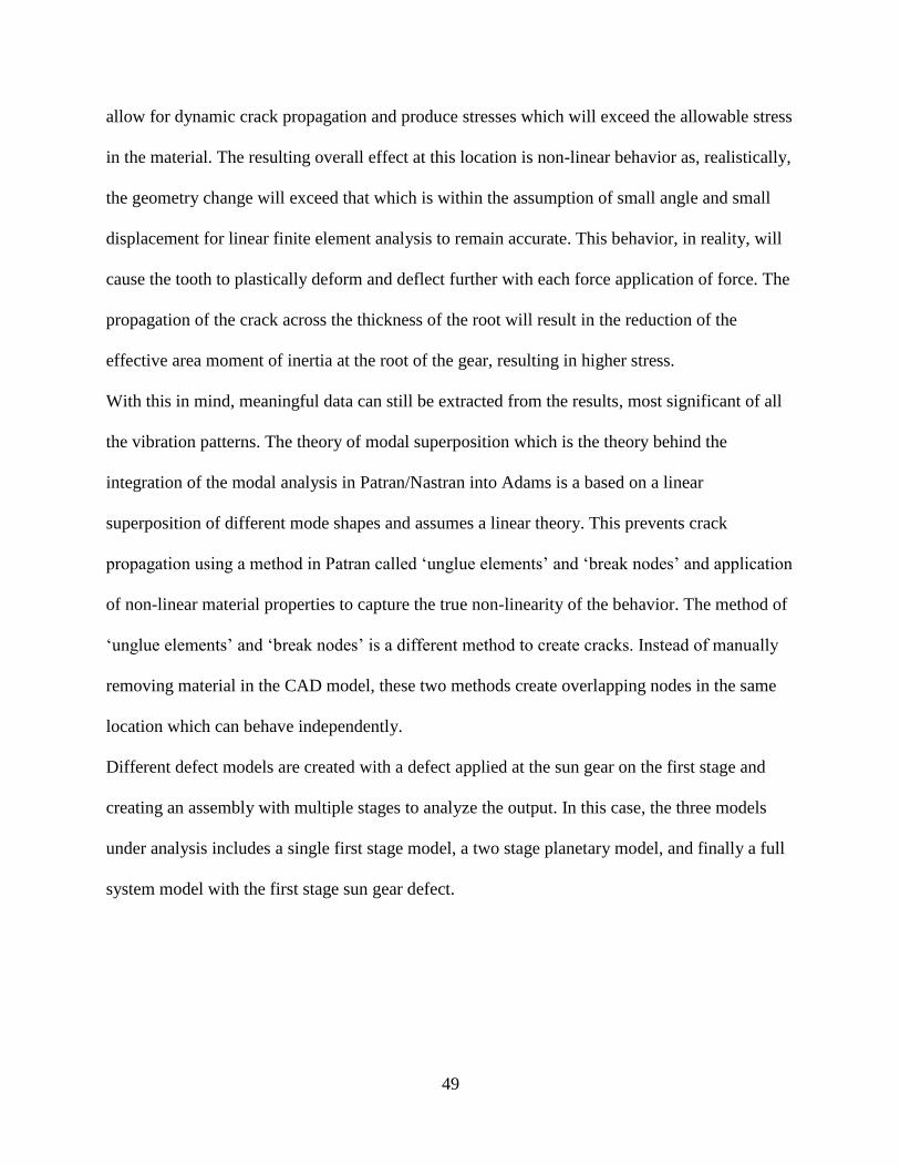
49

allow for dynamic crack propagation and produce stresses which will exceed the allowable stress

in the material. The resulting overall effect at this location is non-linear behavior as, realistically,

the geometry change will exceed that which is within the assumption of small angle and small

displacement for linear finite element analysis to remain accurate. This behavior, in reality, will

cause the tooth to plastically deform and deflect further with each force application of force. The

propagation of the crack across the thickness of the root will result in the reduction of the

effective area moment of inertia at the root of the gear, resulting in higher stress.

With this in mind, meaningful data can still be extracted from the results, most significant of all

the vibration patterns. The theory of modal superposition which is the theory behind the

integration of the modal analysis in Patran/Nastran into Adams is a based on a linear

superposition of different mode shapes and assumes a linear theory. This prevents crack

propagation using a method in Patran called ‘unglue elements’ and ‘break nodes’ and application

of non-linear material properties to capture the true non-linearity of the behavior. The method of

‘unglue elements’ and ‘break nodes’ is a different method to create cracks. Instead of manually

removing material in the CAD model, these two methods create overlapping nodes in the same

location which can behave independently.

Different defect models are created with a defect applied at the sun gear on the first stage and

creating an assembly with multiple stages to analyze the output. In this case, the three models

under analysis includes a single first stage model, a two stage planetary model, and finally a full

system model with the first stage sun gear defect.

50

Figure 29. Defect parameters dimensions

Figure 29 shows the dimensions for the notch which is applied at the root of the gear tooth. This

notch has length 25% of the root thickness of the tooth, in this case the root thickness is 20mm

and the notch length is 5mm. The notch has a slight curvature and is created with an offset inside

of Solidworks. The thickness of the notch is made to be 10% of the length across the tooth face.

5.2 ADAMS VIEW FLEX

As mentioned in the Introduction, an Adams module is available for use which generates a

flexible body without having to import a modal neutral file. Adams View Flex uses a basic

internal meshing software which generates its own .mnf file through Nastran. View flex is used

to general a flexible model to compare the results to Patran/Nastran. A full tutorial on the

development of a flexible body through View Flex can been seen in Appendix 2.

View flex acts similarly as Patran does and can be treated as simply a different, simpler meshing

software.

There are a number of limitations to the View Flex module in Adams. The overall basic meshing

interface allows for the global element definition of the mesh to be defined. For gear model such

51

as the one under analysis, there are two methods of meshing the part to obtain accurate stress

representation; a biased mesh (the method that has been outline in Patran) or a fine mesh on the

entire gear body. If high performance hardware were available to perform an analysis on a full

body fine mesh on a gear tooth and body, this would not be a major concern. However, as an

underlying goal in this analysis, developing a simplified model is meant to reduce computational

time and increase analysis efficiency. Not only would the modal neutral file creation from View

Flex take a significant amount of time, the dynamic simulation for a full stage assembly would

also require a significant amount of time. The idea of meshing an entire gear body to such a

refined mesh so as to match that required at the root of a tooth or the notch radius, would be

highly inefficient. The meshing module for View Flex is shown in Figure 30.

52

Figure 30. Adams Flex Control Module View

The meshing module includes the basic options to create a finite element model. As can be seen,

the meshing module does not allow for the level of mesh refinement which can be achieve by a

full FEA program. The element size selected was 5mm, a minimum size of 1mm with a growth

rate of 1mm. It is clear here that the minimum edge size is insufficient to capture the stress as

previously analyzed by Abaqus convergence study.

For a more simplified geometry, View Flex can be ideal for obtaining a rough benchmark for

analysis. This is similar to the meshing module for Solidworks. However, when a specific mesh

is required with different partitions or seed biases a full FEA software is the better choice. With

the right hardware resources however, View Flex may be able to generate a full body mesh to

analyze. A full body mesh would allow for an accurate representation of the stress profile but it

is an inefficient use of time and resources. Although the analysis of a simulation with View Flex

53

will not be used to create a meaning full comparison with final results, a tutorial on View Flex

can be found in Appendix 2.

54

CHAPTER 6. RESULTS

6.1 GEAR RATIO VERIFICATION

The models generated in Adams allow for a multibody dynamic analysis of the system. In this

case the gear system can be analyzed using a variety of parameters including a flexible body for

stress analysis. The goal of the gear system analysis is to discover the vibration patterns from

different stages of the planetary gearbox. The vibration pattern analyzed through a Fast Fourier

Transform (FFT) plot will show different amplitudes and of certain vibrational frequencies

resulting from a defect in a certain area of the gearbox.

The first test performed in Adams was to simply simulate the results of the predicted angular

velocities of each critical component to determine if they match those predicted by the design

parameters. Table 11 shows the predicted rotational velocity of each component.

Table 11. Calculated Component Velocities

Stage 1 Stage 2 Stage 3

Sun 10.134 112.10 -

Planet 2.695 12.370 -

Carrier 1.76 10.134 -

Ring 0 0 -

Gear - - 112.08

Pinion - - 140.10

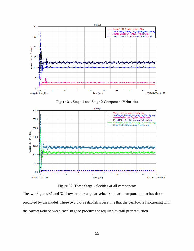
55

Figure 31. Stage 1 and Stage 2 Component Velocities

Figure 32. Three Stage velocities of all components

The two Figures 31 and 32 show that the angular velocity of each component matches those

predicted by the model. These two plots establish a base line that the gearbox is functioning with

the correct ratio between each stage to produce the required overall gear reduction.

56

6.2 STRESS ANALYSIS - STATIC

As a preliminary stress results on the gear tooth were analyzed to capture a static behavior of a

gear tooth under load with different defect sizes at the root. It must first be indicated that this

analysis was performed in Abaqus incorporating non-linear material properties and behavior of

the associated gear tooth. The non-linearity of the behavior of the material must be accounted for

when analyzing failure from defects. The non-linear properties for the gear tooth material is

presented in Figure 33.

Figure 33. AISI 4820 Steel Estimated Non-Linear Stress vs. Strain Relationship

The following plastic deformation properties were applied to the material in anticipation to

capture material failure behavior. This plot was determined using the yield and ultimate stress as

the critical locations with the combination of interpolation to other similar materials

A set of static loading case was applied to the gear too with different notch lengths at the root.

The following results are presented bellow in as Table 12.

0

100

200

300

400

500

600

700

800

900

1000

0 2 4 6 8 10 12 14

Stre

ss [

MP

a]

Strain [%]

57

Table 12. Static Analysis of a Sun Gear Tooth with varying defect size.

Root Notch Stress Location

Comments Left Right Contact Notch Disp

[%] [MPa] [mm]

none 361 312 366 0.024 Elastic (operating

conditions) SF 1.25

25 455 140 302 726 0.035 Yield at notch plastic

deformation.

50 478 65 360 896 0.072 Yield notch and left

fillet.

In Table 12, the stress was measured using the Von Mises stress criteria at different locations on

the gear tooth. These three locations include the left and right root of the gear tooth, the defect

location, and the simulated “contact” location. The application of the contact load is applied as

pressure over a contact patch. Figure 34 and 35 shows a depiction of one of the test cases.

Figure 34. 25% Root Notch Deformed Body Front View

58

Figure 35. 25% Root Notch Deformed Body Notch View

From Figures 34 and 35, the stress contour shows the three high stress location being the notch,

the compression root location and the contact patch. It must be noted that the contact stress

measurement must be read with caution. The FE program simulates a distributed pressure load as

a series of point loads on a surface. The error associated with applied point loads is areas of

infinite stress at the node of application. However, as the distance between the point of interest

and the location of load application the solution converges rapidly [22]. Therefore, the true

contact stress at the location may not be accurately capture by the FE model results.

From the first application of a defect at the root, the results show that material failure occurs at

the notch location. TBC

6.3 STRESS ANALYSIS – DYNAMIC

The FE model creation was developed by Patran using the modal superposition model. The most

significant factor in the stress analysis of the dynamic model is the non-representation of the

non-linearity of the system. The static model is able to account for material non-linearity which

59

is not available to modal superposition. Therefore, stresses measured in the dynamic model

around or greater than the allowable yield stress must be taken with care.

The stress analysis at the root of the gear tooth can be performed under dynamic loading the gear

tooth with the integration of the flexible body into Adams. The flexible body created was the sun

gear on the first stage of the planetary system. The selection for one the stress location is shown

in Figures 36 and 37.

Figure 36. Stress node probing in Adams

60

Figure 37. Stress node probe location 2

Using the Durability module in Adams, the stress locations can be probed in Adams and plotted

as a function of time or another independent variable. The stress contour plot for a healthy tooth

on the sun gear is shown in Figure 38.

61

Figure 38. Stress contour plot in Adams

Figure 38 shows the plot for the maximum principle stress contour plot of the sun gear.

Displaying the maximum principle stress shows the tensile stress incurred on one of the roots of

the gear. The tensile and compressive stress is expected to be different on the gear. The three

stresses probed at these various locations are the maximum principle stress, minimum principle

stress and the Von Mises stress criteria. A general deformation plot is shown in Figure 39.

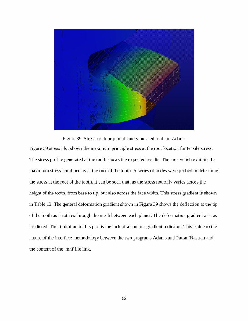
62

Figure 39. Stress contour plot of finely meshed tooth in Adams

Figure 39 stress plot shows the maximum principle stress at the root location for tensile stress.

The stress profile generated at the tooth shows the expected results. The area which exhibits the

maximum stress point occurs at the root of the tooth. A series of nodes were probed to determine

the stress at the root of the tooth. It can be seen that, as the stress not only varies across the

height of the tooth, from base to tip, but also across the face width. This stress gradient is shown

in Table 13. The general deformation gradient shown in Figure 39 shows the deflection at the tip

of the tooth as it rotates through the mesh between each planet. The deformation gradient acts as

predicted. The limitation to this plot is the lack of a contour gradient indicator. This is due to the

nature of the interface methodology between the two programs Adams and Patran/Nastran and

the content of the .mnf file link.

63

Table 13. Stresses at six node locations of the gear tooth from the center to the face

Node

Location

Von

Mises Max Pri. Min Pri.

[N/mm^2]

10706 312.3 -9.87 -351.9

18266 311.8 -9.26 -340.9

20792 239.8 -112.3 -258.2

10355 322.8 361.6 8.27

12869 298.0 333.2 8.45

20437 274.0 295.6 35.29

Figure 40. Minimum principal, compressive, stress from the root center to the face

-390

-340

-290

-240

-190

-140

-90

-40

10

-0.50 0.50 1.50 2.50 3.50 4.50 5.50 6.50

Stre

ss [

N/m

m^2

]

Angle of Rotation (Radians)

RootCompression10706



64

Figure 41.Maximum principal, tensile, stress from the root center to the face

Table 13 indicates nodes with their associated stress probe values measure at an instant in time at

the point of gear teeth contact. The nodes selected were located at the center of the root (10706,

10355), between the face and the center (12869, 18266), and at the edge of the root and the face

(20437, 20792). Figures 40 and 41 shows the stress at the roots of the gear tooth as a single tooth

rotates around one revolution. The force indicated is the maximum and minimum principle

stresses at the root face of the gear, showing root tensile stress and root compression on the

opposite side. It can be seen that, the stress increases as the tooth rotates into contact with each

planet and stress decreases when moving away from the center of the root. The tensile stress is

seen to be slightly greater in magnitude than the compressive stress on the gear root. From the

contour plot off the maximum and minimum principle stress at the root can be observed. The

maximum principle stress at the root is 364.1 MPa and the minimum principle stress at the

-50

0

50

100

150

200

250

300

350

400

-0.50 0.50 1.50 2.50 3.50 4.50 5.50 6.50

Stre

ss [

N/m

m^2

]

Angle of Rotation (Radians)

RootTension10355

RootTension12869

RootTension20437

65

opposite side is -362.4 MPa. The maximum principle stress and the minimum are shown in

Figures 42 and 43.

Figure 42. Maximum principal stress contour plo

Figure 43. Minimum principal stress contour plot

6.4 CONTACT FORCE

The contact force was plotted the series of gear contact locations. These contact locations

includes all contact definition within the Adams model created. The contact force between the

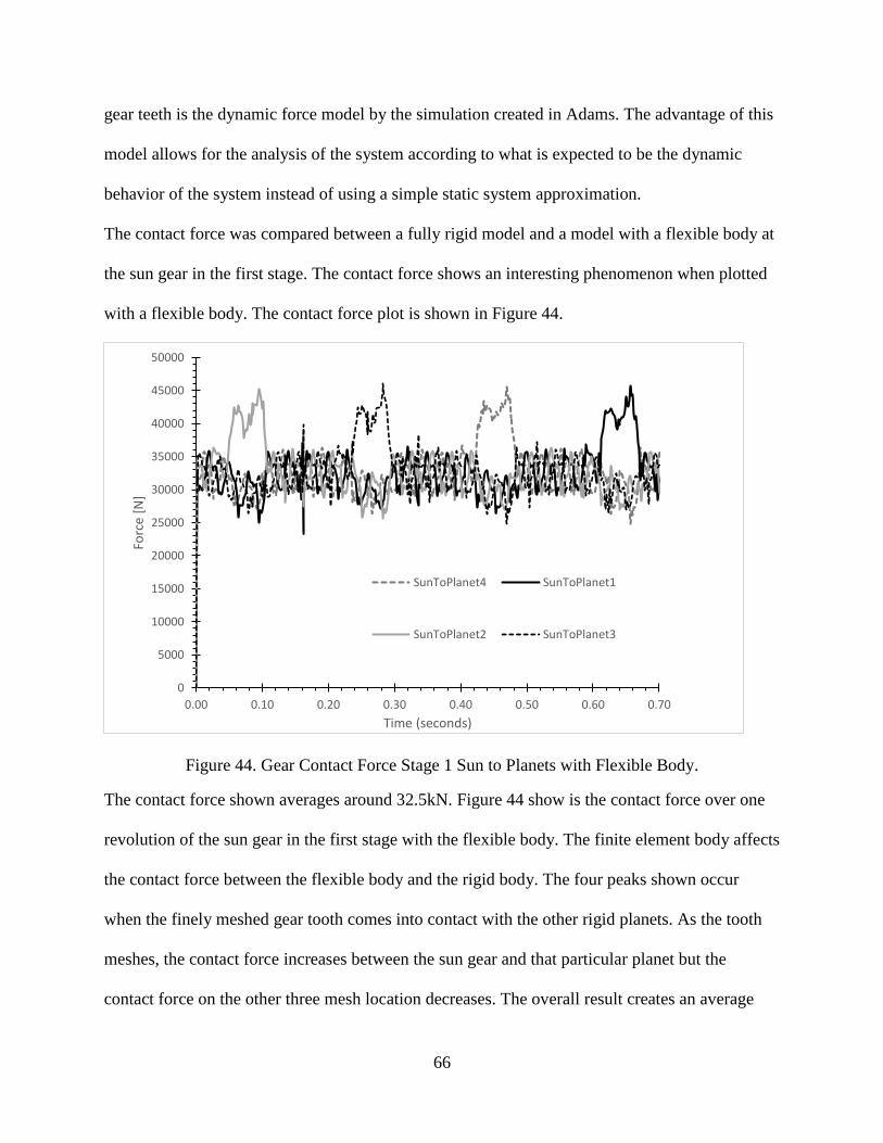
66

gear teeth is the dynamic force model by the simulation created in Adams. The advantage of this

model allows for the analysis of the system according to what is expected to be the dynamic

behavior of the system instead of using a simple static system approximation.

The contact force was compared between a fully rigid model and a model with a flexible body at

the sun gear in the first stage. The contact force shows an interesting phenomenon when plotted

with a flexible body. The contact force plot is shown in Figure 44.

Figure 44. Gear Contact Force Stage 1 Sun to Planets with Flexible Body.

The contact force shown averages around 32.5kN. Figure 44 show is the contact force over one

revolution of the sun gear in the first stage with the flexible body. The finite element body affects

the contact force between the flexible body and the rigid body. The four peaks shown occur

when the finely meshed gear tooth comes into contact with the other rigid planets. As the tooth

meshes, the contact force increases between the sun gear and that particular planet but the

contact force on the other three mesh location decreases. The overall result creates an average

0

5000

10000

15000

20000

25000

30000

35000

40000

45000

50000

0.00 0.10 0.20 0.30 0.40 0.50 0.60 0.70

Forc

e [N

]

Time (seconds)

SunToPlanet4 SunToPlanet1

SunToPlanet2 SunToPlanet3

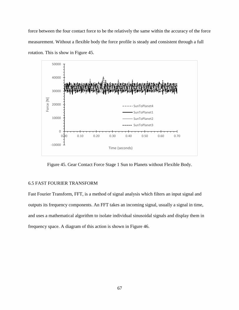
67

force between the four contact force to be the relatively the same within the accuracy of the force

measurement. Without a flexible body the force profile is steady and consistent through a full

rotation. This is show in Figure 45.

Figure 45. Gear Contact Force Stage 1 Sun to Planets without Flexible Body.

6.5 FAST FOURIER TRANSFORM

Fast Fourier Transform, FFT, is a method of signal analysis which filters an input signal and

outputs its frequency components. An FFT takes an incoming signal, usually a signal in time,

and uses a mathematical algorithm to isolate individual sinusoidal signals and display them in

frequency space. A diagram of this action is shown in Figure 46.

-10000

0

10000

20000

30000

40000

50000

0.00 0.10 0.20 0.30 0.40 0.50 0.60 0.70

Forc

e [N

]

Time (seconds)

SunToPlanet4

SunToPlanet1

SunToPlanet2

SunToPlanet3

68

Figure 46. A signal viewed in frequency and time domain [23]

The FFT plot is often used to analyze faults, quality control and condition monitoring of

machines and systems [23]. As can be seen in Figure 46, an arbitrary signal with three

superimposed sinusoidal waves is measured over a period of time shown in red on the left. These

three signals are associated with a specific amplitude and frequency. Using an FFT function on a

processing software the three signals are isolated to produce three individual peaks on a

frequency versus amplitude plot shown as the plot in blue on the right. Peaks at higher

frequencies on a FFT plot can occur at integer multiples of the primary frequency on an FFT, any

other frequencies are considered noise or non-periodic behavior.

The usage of FFT in gear health analysis can be significant since gear contact occurs at specific

frequencies unique to the gear system designed. The frequencies at which gears mesh is defined

as the Gear Mesh Frequency, GMF. The gear mesh frequency can be calculated for each

meshing gear pair as the rotational velocity multiplied by the number of teeth of the gear for a

standard fix axis gear mesh pair. For a planetary gear system, the GMF is defined by the carrier

69

speed multiplied by the number of teeth on the ring gear. There is one specific GMF for each

gear contact which can be calculated from either the pinion or the gear in a fixed axis gear mesh.

In the simulations used for the following analyses, the FFT plot is created using the contact force

between the gears a specified time period. The FFT is used to distinguish a unique vibration

pattern for the planetary gearbox. Frequencies are expected to develop at each specific GMF or

an integer multiple of the GMF, n*GMF. A realistic measurement of gearbox vibration

frequency is to place an accelerometer at each stage on the housing of the system. This allows for

a measurement of the acceleration of the system over time which can then be input to generate an

FFT since measure the contact force directly in a planetary gear system would not be practical.

Gearbox vibration frequency FFTs can indicate defects in the system through a difference in

amplitudes, modulation of the primary GMF, or, but not limited to, the occurrence of sub-

harmonics/super-harmonic frequency peaks. Each different frequency occurrence is associated

with a particular defect which can include, but are not limited to, bearing defect, gear

eccentricity, shaft defect, or gear teeth defect.

6.6 VIBRATION ANALYSIS THROUGH FFT

The first model to be observed is a first stage model with rigid bodies. The model was simulated

for one quarter turn on the input over 2000 steps with an input speed of 1.76 rad/sec. This input

speed corresponds to 16.8RPM which is remains on the high-side of the N90’s operating range

during its low speed operations. This generates over one full revolution on the sun gear output.

The output force was plotted and used to generate the FFT for force in the frequency domain.

This plot is shown as Figure 47.

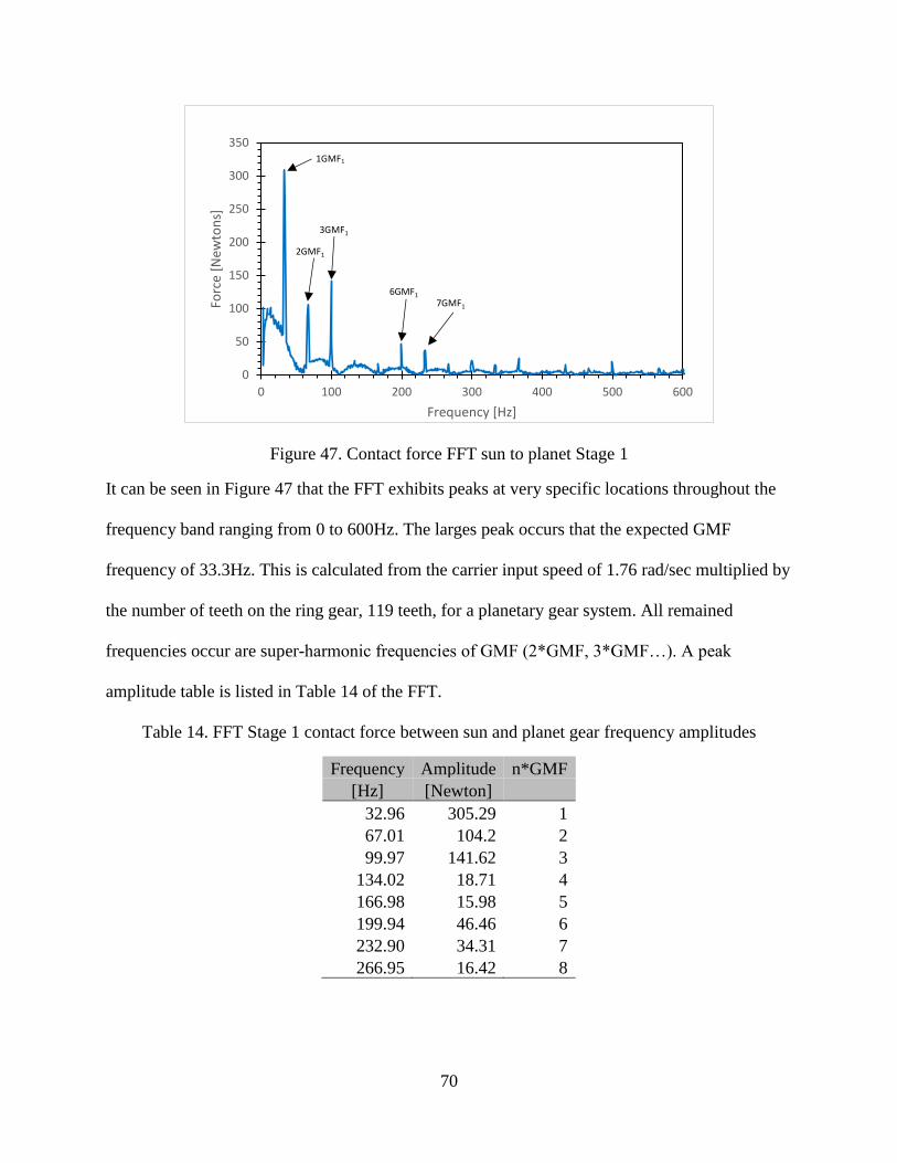
70

Figure 47. Contact force FFT sun to planet Stage 1

It can be seen in Figure 47 that the FFT exhibits peaks at very specific locations throughout the

frequency band ranging from 0 to 600Hz. The larges peak occurs that the expected GMF

frequency of 33.3Hz. This is calculated from the carrier input speed of 1.76 rad/sec multiplied by

the number of teeth on the ring gear, 119 teeth, for a planetary gear system. All remained

frequencies occur are super-harmonic frequencies of GMF (2*GMF, 3*GMF…). A peak

amplitude table is listed in Table 14 of the FFT.

Table 14. FFT Stage 1 contact force between sun and planet gear frequency amplitudes

Frequency Amplitude n*GMF

[Hz] [Newton] 32.96 305.29 1

67.01 104.2 2

99.97 141.62 3

134.02 18.71 4

166.98 15.98 5

199.94 46.46 6

232.90 34.31 7

266.95 16.42 8

0

50

100

150

200

250

300

350

0 100 200 300 400 500 600

Forc

e [N

ewto

ns]

Frequency [Hz]

2GMF1

3GMF1

6GMF1

7GMF1

1GMF1

71

The frequencies demonstrate the vibration pattern generated by such a system at the first stage of

the gearbox. Figure 47 contains points which indicate peaks and its associated GMF harmonic

which corresponds to values in Table 14.

A defect is applied to one of the teeth at the stage one sun gear. The sun gear has been known to

be the most common source of defect occurrence in wind turbine gearboxes. The defect is

imposed at 25% of the root thickness. The same simulation is conducted. The contact force

between the sun gear and the planet gear is taken to generate an FFT plot.

Figure 48. Stage 1 contact force FFT between sun and planet gears with a defect on the sun gear

tooth.

0

50

100

150

200

250

300

350

400

450

500

0 100 200 300 400 500 600

Forc

e [N

ewto

ns]

Frequency [Hz]

1GMF1

2GMF13GMF1

6GMF1

72


gear with and without a defect at the sun gear tooth.

Figure 48 shows the vibration pattern generated by the first stage model with a defect at the first

stage sun gear, points are present to indicate the GMF peaks which are present in the pattern.

Figure 49 represents the superposition of the vibration pattern for the first stage with and without

a defect that the sun gear tooth. The healthy gear FFT is represented by the blue curve and the

defective tooth FFT is represented by the red curve. Table 15 shows the amplitudes of each FFT

plot at the various frequency peaks.

Table 15. Comparison between amplitudes at the GMF harmonics of Stage 1 with and without a

defect at the sun gear tooth.

Frequency GMF

Amp [N] % Change

[Hz] Healthy Defective

32.96 1 305.29 408.14 33.69

67.01 2 104.2 112.57 8.03

99.97 3 141.62 126.59 -10.61

134.02 4 18.71 21.12 12.88

166.98 5 15.98 18.19 13.83

199.94 6 46.46 35.98 -22.56

232.9 7 34.31 26.89 -21.63

0

50

100

150

200

250

300

350

400

450

500

0 100 200 300 400 500 600

Forc

e [N

ewto

ns]

Frequency [Hz]

NoDefect

Defect

1GMF1

2GMF1 3GMF1

6GMF1 7GMF1

73

From both Figure 49 and Table 15, it is shown that there are changes in amplitude at each GMF

on between the healthy and defective models. The most significant impact that can be seen

visually in Figure 49 corresponds to the amplitude change at the primary GMF, 33Hz. This is the

location of the largest peak as well as a 33.7% change in amplitude between the two models.

Although, there are other peaks which exhibit a large amplitude difference, the overall

magnitude of the change is quite small compared to the change at the first GMF.

A similar analysis was performed on the models with a flexible body present as the sun gear with

both healthy and defective tooth. The exact same base model was used, and the meshing was

kept consistent between the two models, however as with different geometry when there is a

defect present versus no defect the meshed model cannot be made the same. The comparison is

show in Figure 50.


gear with and without a defect at the sun gear tooth using flexible bodies.

0

200

400

600

800

1000

1200

1400

0 50 100 150 200 250 300

Forc

e [N

ewto

ns]

Frequency [Hz]

NoDefect

Defect

1GMF1

2GMF1

3GMF1

5GMF1

6GMF1

74


defect at the sun gear tooth using flexible bodies.

Frequency GMF

Amp [N] %

Change [Hz] Healthy Defective

32.96 1 1113.51 1176.7 5.67

66.95 2 336.87 337.12 0.07

99.87 3 264.57 265.84 0.48

166.98 5 105.03 117.44 11.82

199.94 6 113.09 100.65 -11.00

A similar trend is presented in Figure 50 and Table 16. It is seen that there is a noticeable

amplitude change at the primary GMF frequency. The presence of a defect induces a change in

the vibration as can be seen in the FFT of a noticeable magnitude change primarily at the first

GMF for a single stage planetary gear system. In the case of the just analyzing the first stage of

the planetary system by itself, the differences between a healthy and defective gearbox presents

itself through a change in amplitude.

6.7 MULTISTAGE ANALYSIS

The FFT analysis was performed on the system as a whole, involving the three stages put

together as a full assembly. The full system analysis is expected to provide a more realistic

representation of such a system as the N90. This system was simulated with a carrier speed of

1.76 rad/sec (16.8RPM).

75


assembly.

In Figure 51, the contact force at the first stage sun gear was plotted to generate a FFT. The FFT

was generated based on a fully assembled model of the planetary gearbox. The frequencies

present indicated the GMF at the first stage and other super-harmonics with lower amplitude

peaks. However, at 714Hz, there is an amplitude peak present. This peak represents the GMF3

which is the output to the generator.

0

100

200

300

400

500

600

700

800

900

1000

0 200 400 600 800 1000

Forc

e [N

ewto

ns]

Frequency [Hz]

3GMF1

1GMF1

1GMF3

76


assembly.

The second stage FFT, Figure 52, exhibits multiple peaks at a variety of frequencies not unique

to its own stage. The frequency spectrum is dominated by GMF2 however harmonics of GMF1

and GMF3 are represented in the spectrum. The pointers in Figure 52 shows the representations

of these GMF’s.


assembly.

0

200

400

600

800

1000

1200

0 200 400 600 800 1000 1200

Forc

e [N

ewto

ns]

Frequency [Hz]

5GMF1

1/2 GMF3

1GMF2

1GMF3

36GMF1

2GMF2

0

200

400

600

800

1000

1200

0 200 400 600 800 1000 1200

Forc

e [N

ewto

ns]

Frequency [Hz]

1/2 GMF2

14GMF1

3GMF1

29GMF1

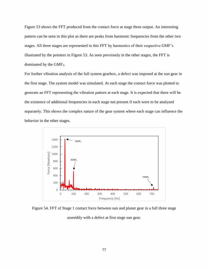
77

Figure 53 shows the FFT produced from the contact force at stage three output. An interesting

pattern can be seen in this plot as there are peaks from harmonic frequencies from the other two

stages. All three stages are represented in this FFT by harmonics of their respective GMF’s

illustrated by the pointers in Figure 53. As seen previously in the other stages, the FFT is

dominated by the GMF3.

For further vibration analysis of the full system gearbox, a defect was imposed at the sun gear in

the first stage. The system model was simulated. At each stage the contact force was plotted to

generate an FFT representing the vibration pattern at each stage. It is expected that there will be

the existence of additional frequencies in each stage not present if each were to be analyzed

separately. This shows the complex nature of the gear system where each stage can influence the

behavior in the other stages.


assembly with a defect at first stage sun gear.

0

200

400

600

800

1000

1200

1400

0 100 200 300 400 500 600 700

Forc

e [N

ewto

ns]

Frequency [Hz]

1GMF1

3GMF1

1GMF3

78



Figure 55 shows the FFT plot for the contact force at the first stage of the gearbox. Similarly to

the isolated analysis of the first stage, it is seen that the presence of a defect appears to only

affect the magnitude of the peaks in the FFT. The comparison between the stages with no defect

versus a defect at the sun gear can be seen at primarily at the GMF1. Table 17 compares the

amplitudes at each frequency.



Frequency GMF

Amp [N] %

Change [Hz] Healthy Crack

32.96 1*GMF1 948.5 1415.4 49.23

99.87 3*GMF1 442.4 521.2 17.81

714.4 1*GMF3 60.43 71.44 18.22

The two changes observed are at 33Hz and 99Hz. This represents behavior at the first stage as a

result of the crack at the first stage sun gear. The other frequency present is the GMF3 seen at

0.00

200.00

400.00

600.00

800.00

1000.00

1200.00

1400.00

0.00 100.00 200.00 300.00 400.00 500.00 600.00 700.00

Forc

e [N

ewto

ns]

Frequency [Hz]

Defect

NoDefect

1GMF1

3GMF1

1GMF3

79

714Hz. It is not expected that there be significant changes to the amplitude at 714Hz. However,

if changes to the third stage GMF were to occur it is unlikely to be seen as significant compared

to the GMF and 3GMF at Stage 1.



0

200

400

600

800

1000

1200

0 200 400 600 800 1000

Forc

e [N

ewto

ns]

Frequency [Hz]

16GMF11/2 GMF2

5GMF1

1GMF2

1GMF3

22GMF1

2GMF2

32GMF1

10GMF1

80



Figure 56 shows the FFT plot generated from the contact force at stage two between the sun gear

and the planet gear with a defect at the first stage sun gear. Figure 57 shows the superposition of

the FFT with no defect (blue) and a defect at the first stage sun gear (red). Pointers in Figure 57

highlight appearances of certain frequencies in the defective gearbox not seen in the non-

defective assembly. In Figure 57, the three indicated peaks representing harmonics of GMF2 and

GMF3 are modulated by higher harmonics of GMF1. The frequency difference is expressed in

Table 18.



Frequency GMF

Amp [N] %


519.8 1GMF2 925.7 1005.6 8.63

535.0 16GMF1 15.1 118.3 683.4

714.1 1GMF3 350.1 331.7 -5.26

732.4 22GMF1 18.78 91.6 387.5

1038.0 2GMF2 363.2 402.5 10.8

1064.4 32GMF1 9.43 283.3 2904

0.00

200.00

400.00

600.00

800.00

1000.00

1200.00

0.00 200.00 400.00 600.00 800.00 1000.00

Forc

e [N

ewto

ns]

Frequency [Hz]

Defect

NoDefect

1GMF2

16GMF1

1GMF3

22GMF1

32GMF1

2GMF2

81

Table 18 shows the three large peaks of GMF2 and GMF3 modulated by GMF1 harmonics. In this

case, it can be suspected that this maybe the indication of a vibration signature of a defect at the

first stage sun gear represented through the second stage FFT analysis, the development of a

vibration pattern will be discussed further in the next section.



0

200

400

600

800

1000

1200

0 200 400 600 800 1000

Forc

e [N

ewto

ns]

Frequency [Hz]

3GMF1

22GMF1

1GMF3

1GMF3 + 3GMF1

25GMF16GMF1 1GMF2

1GMF3 - 3GMF1

0

200

400

600

800

1000

1200

0 200 400 600 800 1000

Forc

e [N

ewto

ns]

Frequency [Hz]

Defect

NoDefect

22GMF1

1GMF3

25GMF1

1GMF3 + 3GMF1

1GMF3 - 3GMF1

82



Figure 58 shows the FFT vibration pattern for the third stage with a defect at the first stage sun

gear. Figure 59 shows the superposition of the FFT from both a defective and a non-defective

gearbox. The third stage FFT shows significant changes in the frequency patterns between the

two gearboxes. Figure 58 shows the variation of GMF’s between all three stages which are

present in the FFT. Figure 59 highlights the significant occurrences of the frequencies which

appear due to the defect. It can be seen that sideband frequencies appear at both a higher and

lower frequency to the dominant GMF3. Sideband frequencies occur at 1GMF3 - 3GMF1 and

1GMF3 + 3GMF1. Along with the sideband frequencies, modulation of these GMF3 and the

sidebands by harmonics of the GMF1 can be seen. It can also be noted that the sideband

frequency of 1GMF3 occurs at 1GMF3 plus the second dominant frequency, 3GMF1, seen at the

first stage FFT. These significant GMF are presented in Table 19.


defect at the sun gear tooth

Frequency GMF

Amp [N] %


614.8 1GMF3 - 3GMF1 48.55 221.9 357.1

714.1 1*GMF3 974.3 987.6 1.37

731.4 22*GMF1 27.3 257.1 541.8

813.2

1GMF3 +

3GMF1 18.31 482.6 2530

831.6 25*GMF1 46.9 628.6 1667

83

6.8 VARYING INPUT SPEED VIBRATION TESTS

The first set of simulations in Adams were performed at steady state conditions using an input

velocity at the first stage of 1.76 rad/sec. The same analysis was performed on the model at two

different speeds above and below 1.76 rad/sec. The speeds chosen were 1.5 rad/sec and 2.0

rad/sec. As a result of the change of input speed the GMF of each system will change

accordingly the expected base GMF for both systems are shown in Table 20.

Table 20. Base Gear Mesh Frequencies for different speed input

Speed GMF

[Hz]

[rad/sec] S1 S2 S3

1.5 28.4 443 608

2 37.9 590 811

The speed variation is performed so that the vibration signature pattern can be determined for a

defect at the first stage sun gear. The speeds selected for these two tests are within the range of

operation of the N90. A speed of 1.50 rad/sec is equivalent to 14.3RPM, this is in the mid

operating range of the N90. An input speed of 2.0 rad/sec corresponds to 19.1RMP which is with

in one the high end of the operating range during high speed operations of the N90.

The following figures, Figure 60, Figure 61 and Figure 62 show the FFT for at Stage 1 of the

contact force between the sun and the planet gear with and without a defect at the first stage sun

gear tooth for an input speed of 1.5 rad/sec (14.3RPM).

84


assembly with input speed 1.5 rad/sec.


assembly with a defect at first stage sun gear with input speed 1.5 rad/sec.

0

100

200

300

400

500

600

700

800

900

0 100 200 300 400 500 600 700 800

Forc

e [N

ewto

ns]

Frequency [Hz]

1GMF1

5GMF1

1GMF3

0

100

200

300

400

500

600

700

800

900

1000

0 100 200 300 400 500 600 700 800

Forc

e [N

ewto

ns]

Frequency [Hz]

1GMF1

5GMF1

1GMF3

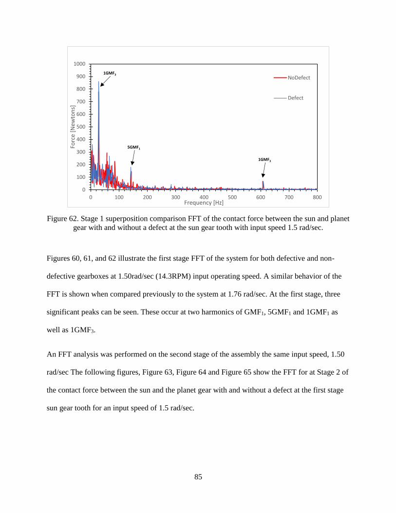
85


gear with and without a defect at the sun gear tooth with input speed 1.5 rad/sec.

Figures 60, 61, and 62 illustrate the first stage FFT of the system for both defective and non-

defective gearboxes at 1.50rad/sec (14.3RPM) input operating speed. A similar behavior of the

FFT is shown when compared previously to the system at 1.76 rad/sec. At the first stage, three

significant peaks can be seen. These occur at two harmonics of GMF1, 5GMF1 and 1GMF1 as

well as 1GMF3.

An FFT analysis was performed on the second stage of the assembly the same input speed, 1.50

rad/sec The following figures, Figure 63, Figure 64 and Figure 65 show the FFT for at Stage 2 of

the contact force between the sun and the planet gear with and without a defect at the first stage

sun gear tooth for an input speed of 1.5 rad/sec.

0

100

200

300

400

500

600

700

800

900

1000

0 100 200 300 400 500 600 700 800

Forc

e [N

ewto

ns]

Frequency [Hz]

NoDefect

Defect

1GMF3

5GMF1

1GMF3

86





0

100

200

300

400

500

600

700

800

900

1000

0 100 200 300 400 500 600 700 800 900 1000

Forc

e [N

ewto

ns]

Frequency [Hz]

7GMF1

1GMF2

1GMF3

27GMF1

2GMF2

1/2 GMF2

0

100

200

300

400

500

600

700

800

900

1000

0 100 200 300 400 500 600 700 800 900 1000

Forc

e [N

ewto

ns]

Frequency [Hz]

1GMF2

14GMF117GMF1

1GMF3

22GMF1

2GMF2

32GMF1

7GMF1

9GMF1

87



Figures 63, 64, and 65 show the FFT at the second stage with and without a defect at the first

stage sun gear. In Figure 65, the comparison between the two FFT’s shows modulation of

1GMF2, 2GMF2 and 1GMF3 by harmonics of GMF1. Two first stage harmonics modulate the

dominate 1GMF2 and one GMF1 harmonic modulates 1GMF3 and 2GMF2. The similar

occurrence to the system at 1.76 rad/sec is the modulation of 1GMF2 and 1GMF3. This can be

determined as possible vibration signature to the defect.

The following figures, Figure 66, Figure 67 and Figure 68 show the FFT for at Stage 3 of the

contact force between the sun and the planet gear with and without a defect at the first stage sun

gear tooth for an input speed of 1.5 rad/sec.

0

100

200

300

400

500

600

700

800

900

1000

0 100 200 300 400 500 600 700 800 900 1000

Forc

e [N

ewto

ns]

Frequency [Hz]

NoDefect

Defect

1GMF2

14GMF117GMF1

1GMF3

22GMF1

2GMF2

32GMF1

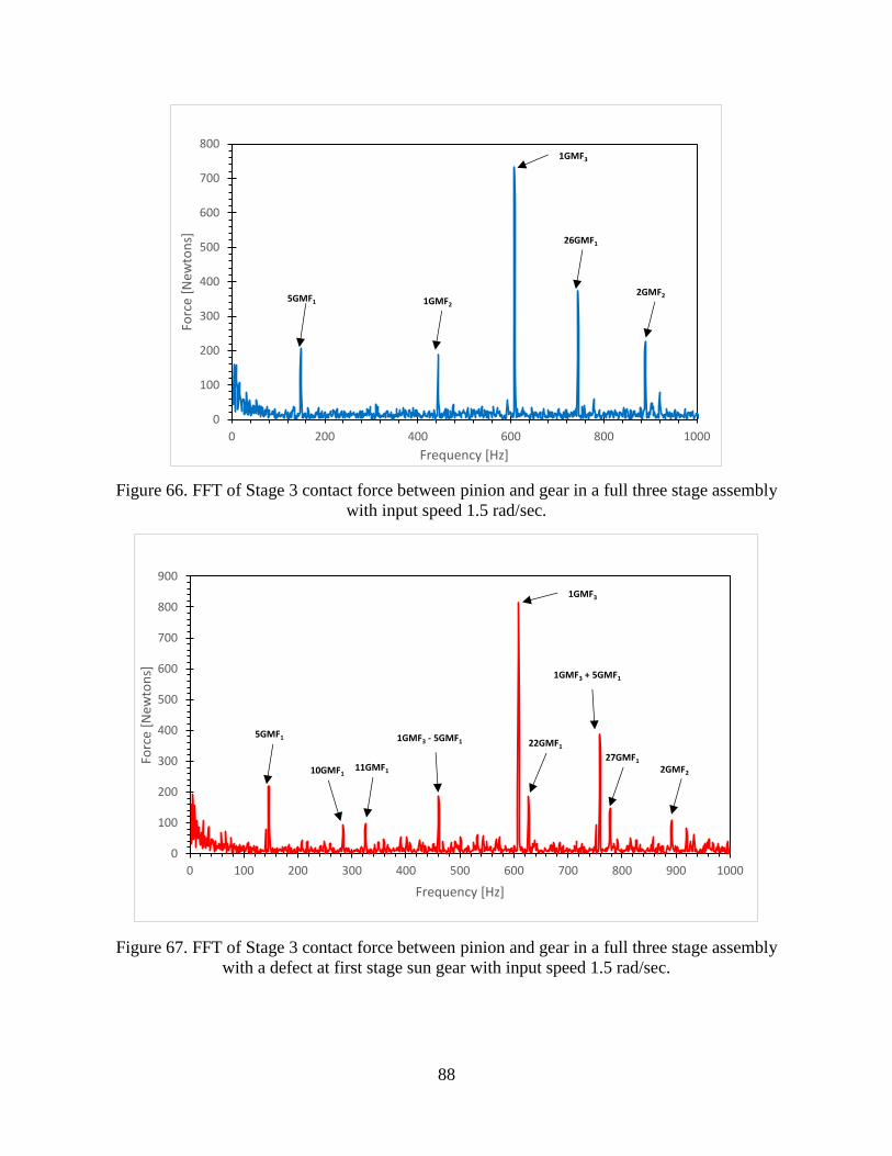
88


with input speed 1.5 rad/sec.


with a defect at first stage sun gear with input speed 1.5 rad/sec.

0

100

200

300

400

500

600

700

800

0 200 400 600 800 1000

Forc

e [N

ewto

ns]

Frequency [Hz]

5GMF1 1GMF2

1GMF3

26GMF1

2GMF2

0

100

200

300

400

500

600

700

800

900

0 100 200 300 400 500 600 700 800 900 1000

Forc

e [N

ewto

ns]

Frequency [Hz]

5GMF1 1GMF3 - 5GMF1

1GMF3

22GMF1

27GMF1

1GMF3 + 5GMF1

2GMF210GMF111GMF1

89



Figures 66, 67, and 68 show the FFT vibration pattern at the third stage with and without the

defect at stage one sun gear. The superposition plot, Figure 68, highlights the significant peaks

seen as the defect is imposed on the first stage sun gear. At the third stage FFT, it can be seen

that sideband frequencies occur from the dominant 1GMF3 at both a lower and higher frequency.

The sideband frequencies which are present are 1GMF3 - 5GMF1 and 1GMF3 + 5GMF1.

Frequency modulation of the dominant 1GMF3 and the higher sideband, 1GMF3 + 5GMF1, by

harmonics of GMF1 is seen. It can also be noted that the sideband frequencies of 1GMF3 occurs

at 1GMF3 plus/minus the second dominant frequency, 5GMF1, seen at the first stage FFT. This

pattern is similar to the system at 1.76 rad/sec.

The same simulation was performed on the system with a higher input speed at 2.0 rad/sec. The

FFT at the three stages were generated to define a vibration signature for this particular tooth

defect at the first stage sun gear. The following figures, Figure 69, Figure 70 and Figure 71 show

0

100

200

300

400

500

600

700

800

900

0 100 200 300 400 500 600 700 800 900 1000

Forc

e [N

ewto

ns]

Frequency [Hz]

NoDefect

Defect

1GMF3 - 5GMF1

1GMF3

22GMF1

27GMF1

1GMF3 + 5GMF1

90

the FFT for at Stage 1 of the contact force between the sun and the planet gear with and without

a defect at the first stage sun gear tooth for an input speed of 2.0 rad/sec (19.1RPM).



0

200

400

600

800

1000

1200

0 100 200 300 400 500 600 700 800 900

Forc

e [N

ewto

ns]

Frequency [Hz]

1GMF1

1GMF3

91





0

200

400

600

800

1000

1200

1400

0 100 200 300 400 500 600 700 800 900

Forc

e [N

ewto

ns]

Frequency [Hz]

1GMF1

2GMF1

1GMF3

3GMF1

4GMF1

0

200

400

600

800

1000

1200

1400

0 100 200 300 400 500 600 700 800 900

Forc

e [N

ewto

ns]

Frequency [Hz]

NoDefect

Defect

1GMF1

2GMF1

1GMF3

3GMF1

4GMF1

92

Figures 69, 70, and 71 shows the first stage FFT of the system with and without a defect at the

first stage sun gear at 2.0 rad/sec (19.1RPM) input operating speed. A similar behavior of the

FFT is shown when compared previously to the system at 1.76 rad/sec. At the first stage, two

significant peaks can be seen on a non-defective gearbox at 1GMF1 and 1GMF3. On the

defective gearbox more significant peaks occur at four harmonics of 1GMF1, 2GMF1, 3GMF1,

4GMF1 and 1GMF3 as well as other GMF1 harmonics at a much lower amplitude when

compared to the first four of GMF1. The superposition plot, Figure 71, shows these significant

peaks.

As with the other two operating speeds, the second stage FFT is generated. The following

figures, Figure 72, Figure 73 and Figure 74 show the FFT for at Stage 2 of the contact force

between the sun and the planet gear with and without a defect at the first stage sun gear tooth for

an input speed of 2.0 rad/sec.

93





0

100

200

300

400

500

600

700

800

900

0 100 200 300 400 500 600 700 800 900

Forc

e [N

ewto

ns]

Frequency [Hz]

1/4 GMF1

8GMF1

3GMF1

1GMF3

0

100

200

300

400

500

600

700

800

900

1000

0 100 200 300 400 500 600 700 800 900

Forc

e [N

ewto

ns]

Frequency [Hz]

14GMF1

1GMF1

1GMF2

17GMF1

21GMF1

1GMF33GMF1

94



Figures 72, 73, and 74 show the FFT at the second stage with and without a defect at the first

stage sun gear. In Figure 74, the comparison between the two FFT’s shows modulation of

1GMF2 and 1GMF3 by harmonics of GMF1. The dominant peak, 1GMF2 is modulated by two

GMF1 harmonics, 14GMF1 and 17GMF1. The third stage GMF, 1GMF3, is modulated by

21GMF1. The similar occurrence to the system at 1.50 rad/sec and 1.76 rad/sec is the modulation

of 1GMF2 and 1GMF3 by harmonics of GMF1. From the three different speed test, the

modulation of 1GMF2 and 1GMF3 by harmonics of GMF1 can be determined as a vibration

signature at the second stage of this three stage system with a defect on the tooth of the first stage

sun gear.

As with the other system speed tests, this system is simulated at 2.0 rad/sec and the third stage

FFT is developed. The following figures, Figure 75, Figure 76 and Figure 77 show the FFT for at

0

100

200

300

400

500

600

700

800

900

1000

0 100 200 300 400 500 600 700 800 900

Forc

e [N

ewto

ns]

Frequency [Hz]

NoDefect

Defect

14GMF1

1GMF2

17GMF121GMF1

1GMF3

95

Stage 3 of the contact force between the pinion and the gear with and without a defect at the first

stage sun gear tooth for an input speed of 2.0 rad/sec.


with input speed 2.0 rad/sec.

0

100

200

300

400

500

600

700

800

900

1000

0 100 200 300 400 500 600 700 800 900

Forc

e [N

ewto

ns]

Frequency [Hz]

3GMF1 1/4GMF3

12GMF1

1GMF2

19GMF1

1GMF3

96


with a defect at first stage sun gear with input speed 2.0 rad/sec.



0

100

200

300

400

500

600

700

800

0 100 200 300 400 500 600 700 800 900

Forc

e [N

ewto

ns]

Frequency [Hz]

3GMF11/4GMF3

22GMF1

24GMF1

19GMF1

1GMF3

1GMF3 + 3GMF1

0

100

200

300

400

500

600

700

800

900

1000

0 100 200 300 400 500 600 700 800 900

Forc

e [N

ewto

ns]

Frequency [Hz]

NoDefect

Defect

22GMF1

24GMF1

19GMF1

1GMF3

1GMF3 + 3GMF1

97

Figures 75, 76, and 77 show the FFT vibration pattern at the third stage with and without the

defect at stage one sun gear. The superposition plot, Figure 77, highlights the significant peaks

seen as the defect is imposed on the first stage sun gear. A sideband frequency occurs from the

dominant 1GMF3 at a higher frequency. The sideband frequency which is present is 1GMF3 +

3GMF1. Frequency modulation of the dominant 1GMF3 and the higher sideband, 1GMF3 +

3GMF1, by harmonics of GMF1 can be seen to occur. The sideband frequency present in this

FFT, occurs at 1GMF3 + 3GMF1, 3GMF1 is one of the significant frequencies which occurs at

when looking the first stage FFT of the system. This pattern is similar to the system at both 1.50

rad/sec and 1.76 rad/sec. This pattern can be determined as vibration signature seen at the third

stage FFT of a full system assembly due to a defect at the first stage sun gear.

98

CHAPTER 7. CONCLUSION

The vibration signature for a three stage wind turbine gearbox representing the Nordex N90 with

a defect was developed. With the methods outlined in this these for incorporating a flexible body

through the use of MSC Patran/Nastran into Adams. The stress at a desired location can be

acquired under the dynamic operations of the system which is more realistic as to the more

classical static stress analysis or impact analysis in the classical FEA software. The use MSC

Patran/Nastran allows for the ease of integration between the finite element model into a

dynamic system. The method of development for the vibration characteristics of this system

developed in this thesis can be used to further study and simulated a variety of cases and defects

which can occur in a wind turbine gearbox.

The strength MSC Adams is highlighted by the ability to simulate dynamic interaction between

bodies and generate vibration results and stress results due to the integration of a flexible body.

This allows for the first steps in a development of a health monitoring method for a gearbox. In

this case, the targeted gearbox is the Nordex N90 wind turbine. With the availability of the

working hardware, a significant limitation is the computational time required for simulations.

Model scale reduction was used for computational efficiency purposes in the simulations.

Limitations to stress analysis to defects such as the one investigated in this thesis is the method

in which the flexible body is generated for integration into MSC Adams from MSC Patran. The

Craig-Bampton modal analysis used on the body is a linear superposition of modes. This method

only captures the linear behavior of the system and cannot be used with non-linear analysis

methods, as confirmed when discussing with a Patran expert at MSC. This means that non-linear

geometry or material behavior cannot be captured through this method of dynamic stress

analysis. In terms of defects at the gear teeth root, the defect model represented in this research is

99

a notch model created at the root of the tooth. This can be representative of a crack which has

occurred at the root. MSC Patran has the capability to perform crack propagation methods which

would generally be ideal for such an analysis. However, crack propagation through ungluing

elements, as it is referred to in Patran, is a non-linear method and is not compatible with the

Craig-Bampton method.

With the methods developed in this thesis, it is hopeful that further research can be conducted

into gearbox health monitoring with a variety of different types of defects and integration of

different elements seen in a typical system. The model for the N90 gearbox is developed based

on previous research on this wind turbine as with limited information provided by Nordex

themselves, in the hopes of creating a model which can be representative of the true N90 system.

However, without a schematic provided by Nordex, it would be impossible to create a perfect

representation.

There are certain aspects with both MSC Adams and MSC Patran that may defer other uses from

utilizing the full strength of the software. The most challenging aspect to navigate around is the

user interface (UI) of both software. A tutorial on gear flexible body development is provided

with this document with the hopes that it will significantly reduce the time to develop a working

system model for further research. Certain aspects of the Adams software are inefficient and

confusing such as developing a working model. With different changes and improvements to the

UI, different processes used in this research can be performed with ease. Both MSC Adams and

Patran are very powerful software especially with multibody dynamic analyses however, a lot of

its capabilities are hidden behind what maybe classified as an outdated user interface when

compared to those of ANSYS, Abaqus, Solidworks, or Creo Direct.

100

REFERENCES

[1] “Nordex N90 Specification Sheet” Nordex SE

[2] Sheng S. “Wind Turbine Gearbox Condition Monitoring Round Robin Study – Vibration

Analysis”, National Renewable Energy Laboratory, 2012.

[3] “Wind Turbine Gear Failure Modes – A Brief”, National Renewable Energy Laboratory

ASME/STLE 2011 International.

[4] Puigcorbe J., and De-Beaumont A., 2010, “WindTurbine Gearbox Reliability: The impact of

rotor support,” Renewable Energy World Magazine.

[5] Norton, Robert L. Machine Design an Integrated Approach. Prentice Hall, 2014.

[6] D. W. Aitken, “Transitioning to A Renewable Energy Future”, ISES White Paper, 2003.

[7] Ribrant J., and Bertling L. M., 2007, “Survey ofFailures in Wind Power Systems With Focus

on Swedish Wind Power Plants During 1997–2005,” IEEE Transactions on Energy

Conversion.

[8] Alemayehu, Fisseha M. and Ekwaro-Osire, Stephen “Loading And Design Parameter

Uncertainty In The Dynamics And Performance Of High-Speed-Parallel-Helical Stage Of

A Wind Turbine Gearbox”

[9] Özgüven and Houser, "Mathematical Models used in Gear Dynamics – A Review," Journal

of Sound and Vibration, no. 121(3).

[10] Smolders K., Long H., Feng Y., and Tavner P., 2010,“Reliability Analysis and Prediction of

Wind Turbine Gearboxes,” European Wind Energy Conference,Warsaw, Poland.

101

[11] Sawatzky, Rene P. D. “Vibration Based Planetary Gear Analysis and Damage Detection”

[12] A. Milburn, "Wind Turbine Gearbox Wear and Failure Modes and Detection Methods,"

2011.

[13] Musial W., Butterfield S., and McNiff B., 2007,“Improving wind turbine gearbox

reliability,” European Wind Energy Conference, Milan, Italy.

[14] Kong, Meagher, Xu, Wu and Wu, "Nonlinear Contact Analysis of Gear Teeth for

Malfunction Diagnostics," IMAC XXVI a Conference on Structural Dynamics, Society for

Experimental Mechanics, 2008.

[15] J. Giesbers, "CONTACT MECHANICS IN MSC ADAMS," University of Twenty, 2012.

[16] Wu, Meagher and Sommer, "A Differential Planetary Gear Model with Backlash and Teeth

Damage," IMAC XXIX a Conference and Exposition on Structural Dynamics, Society for

Experimental Mechanics, 2011.

[17] Bradaric, G. “Dynamic analysis of connecting rods usinc msc adams modal synthesis

method for flexible bodies” 2017

[18] Sommer, Meagher and Wu, "Gear Defect Modeling of a Multiple-Stage Gear Train,"

Modellingand Simulation in Engineering, 2011.

[19] Lin and Parker, "Analytical Characterization of the Unique Properties of Planetary Gear

Free Vibration," ASME Journal of Vibration and Acoustics, 1999.

[20] K. L. Johnson, Contact mechanics, Cambridge: Press Syndicate of the University of

Cambridge, 2004.

102

[21] Verheul, Chris “ADAMS Methodology: Contact Modeling” MSC Software, SayField

International, Lecture.

[22] Spencer, A. J. M. Continuum mechanics. Dover Publications, 2014.

[23] Audio, NTi. "How an FFT works". www.nti-audio.com.

[24] Craig, Roy, and Mervyn Bampton. "Coupling of substructures for dynamic analyses." AIAA

journal 6.7 (1968): 1313-1319.

[25] Alshabatat, Nabeel & Naghshineh, Koorosh. (2014). Optimization of Natural Frequencies

and Sound Power of Beams Using Functionally Graded Material. Advances in Acoustics

and Vibration. 2014. 1-10. 10.1155/2014/752361.

[26] Fundamentals of Structural Dynamics Roy R. Craig… (517 Textbook)

[27] MSC Software Corporation. “Adams Flex Help (for Adams 2017.1).” 23 Mar. 2017.

[28] Ottarson, Gisli, Greg Moore, and Diego Minen. "MDI/ADAMS-MSC/NASTRAN

Integration Using Component Mode Synthesis." (1998).

[29] Budynas Richard G, Nisbett Keith J. “Shigley's Mechanical Engineering Design.”,

McGraw-Hill Education, 1 Jan. 1970.

103

APPENDICES

APPENDIX A - PATRAN TUTORIAL

MSC Patran to Adams Flexible Body Integration for an Output

Gear in a Planetary Gear System Assembly: A Tutorial

Tananant (Mel) Boonya-ananta

[email protected]

Mechanical Engineering Department

California Polytechnic State University

San Luis Obispo, CA 93407

Disclaimer: This tutorial assumes basic knowledge of Solidwork or other CAD software and Adams

View. This document will walk through the process of creating a flexible body in MSC

Patran and a quick note on system integration into MSC Adams.

This tutorial is developed from the Youtube video referenced bellow which creates a similar

analysis using a crank/slider system.

“Flexible Body Integration Using Adams and MSC Nastran”

https://www.youtube.com/watch?v=dd9rjSe27rU

https://www.youtube.com/watch?v=dd9rjSe27rU

104

Tutorial

Prepare a model in Solidworks or other CAD programs and save as a Parasolid file. For the purposes of

this tutorial a model has been provided in the same directory named “Stage1NoCrack.x_t”. Note that .x_t

and .x_b file types are both Parasolid files and will work for this tutorial.

The part is prepartitioned in Soldiworks using the split face tool to generate independent surfaces for

meshing. This is show below.

Start by opening MSC Patran. The icon will look similar, if not exactly the same as this.

Before creating the database for the analysis, it is recommended that the Parasolid file is in the same

working directory (preferably a newly created one), this will ensure that all related files are created and

remain in the same location. This Parasolid file will also be the same file that will be used to create the

model in Adams.

Once Patran is open, navigate to the Home tab and click the “New Database” icon. Name and create the

new database in the working directory. Leave default templates. Click “OK”.

105

106

A right hand side (RHS) window will pop up, accept default settings click “OK”.

Navigate to the “Menu”, a drop down window will

appear. Mouse over “File” and click “Import”.

107

A new window will pop up. Select “Stage1NoCrack.x_t”. This model is created in Metric units under

MMKS unit convention. This indicates that the main unit of length is MILLIMETERS. On the right side

of the import window, click “Parasolid xmt Options…”. A RHS menu will open select “Model

Units…”

Under Model Units change the default Inches to Millimeters

Click “OK” this will bring up a question to confirm the change from inches to millimeters, click “Yes” to

return to the Import options window and click “OK” then “Apply”. This will import in the parasolid

assembly that we have made.

108

Once the model is import, a confirmation window will pop up. Click “OK” to accept the imported

assembly.

The model will import as a wireframe model. Navigate to the top ribbon under the “Display” section

change the view to “Smooth Shaded”.

From here click the “Model Tree” button on the top ribbon to bring up the model tree on the left hand

side (LHS) of the main view window. Under the “Groups” family in the model tree expend the group to

see the different bodies in the model. Uncheck “default_group” and check “SunStage2”

109

This will isolate only the SunStage1 gear. The model viewer should now only have one part in selected

and in view.

To create the Mesh for the part, at the top ribbon select “Meshing”.

The Finite Elements menu will appear in the RHS. In this menu

select, “Mesh” and “Surface” under the Object and Type drop down

menu.

Move down to “Surface List” and select the partitioned root face in

the viewport by using shift click to select multiple surfaces. “Solid

6.3 6.1” should show up in the input box. Under “Global Edge

Length” uncheck Automatic Calculation and change the Value to

“0.125”. Click “Apply”.

110

Element Type

Element Shape

Function

Location

Seed Size

[mm]

Quadrilateral

(2 Dimensional)

Linear

(Quad4)

Root 0.125

Tooth Body 0.5

Gear Body 4

Thickness

Extrusion

5

Perform this action for all the front faces of the gear according to the table shown above for mesh

parameters.

The meshed is shown below:

To extrude the mesh to the rest of the body under “Action” select “Sweep” and under “Method” select

“Extrude”. The direction vector to “<0 0 -1>” and the extrude distance to “5” with and offset of “0.0”.

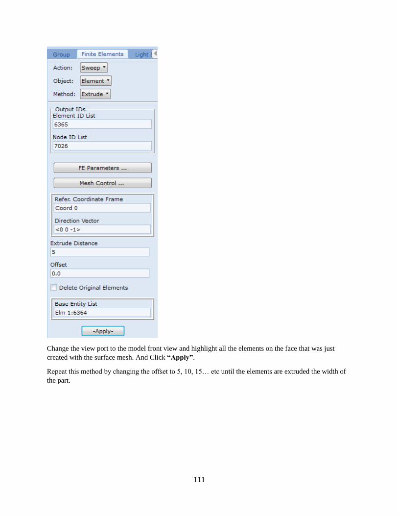
111

Change the view port to the model front view and highlight all the elements on the face that was just

created with the surface mesh. And Click “Apply”.

Repeat this method by changing the offset to 5, 10, 15… etc until the elements are extruded the width of

the part.

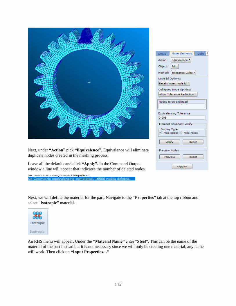
112

Next, under “Action” pick “Equivalence”. Equivalence will eliminate

duplicate nodes created in the meshing process.

Leave all the defaults and click “Apply”. In the Command Output

window a line will appear that indicates the number of deleted nodes.

Next, we will define the material for the part. Navigate to the “Properties” tab at the top ribbon and

select “Isotropic” material.

An RHS menu will appear. Under the “Material Name” enter “Steel”. This can be the name of the

material of the part instead but it is not necessary since we will only be creating one material, any name

will work. Then click on “Input Properties…”

113

A new window will pop up named Input Options. Here we will enter the material properties of our gear

steel. Note that the units must remain consistent. In this case, MMKS. Click “OK”. To return to the

Materials RHS menu then click “Apply”.

114

Once the material has been created the material named “Steel” should show up in the LHS model tree.

Now we will apply the material to the body. Under the same Properties tab in the top ribbon click

“Solid”.

115

A RHS menu will pop up named Element Properties. Enter a property set name “gearProp” then click on

Input Properties.

A new window will appear:

116

Click on the square symbol marked in the right green circle and select the material we created “Steel”.

Under Material Name, the box should be filled with “m:Steel” as shown above with the left green circle.

Click “OK”. This will return the the RHS Element Properties menu. At the bottom click “Select

Application Region…”.

On the Right tab of the viewport, select “View Solid Elements” .

117

In the new RHS window under select members click the gear in the viewport and Elm 6365:44548 should

appear in the text box. Click “Add” this will add it to the Application Region window below then Click

“OK” then “Apply”.

“gearProp” will appear in the Model Tree on the LHS under Properties:

Now we will apply the nodes where this gear is to be constrained, the points where bearings will ideally

exist. Under the Home tab on the top ribbon, a wireframe view, erased FEM and large point size will

make this process easier.

The model in the viewport should look like this after those 3 changes:

118

Navigate to the Geometry tab at the top ribbon, a new RHS menu will pop up. Under “Method” change

XYZ to “ArcCenter”. With Auto Execute checked click on the curve that represents the inside edge of

the gear.

Repeat this step for 3 other locations. The final product should look like this:

119

Now, we will interpolate between the points to create a point at the center of the gear. Under “Method”

change ArcCenter to “Interpolate”. At the bottom, select two of the points created to interpolate between

them.

120

121

These points will act as reference points. Now that they have been created, under “Menu” ➔ “Utilities”

select “FEM-General” ➔ “RBE2/RBE3 Spider …”

122

RBE2/RBE3 Spider Menu will pop up on the RHS menu. Here we will select all Dependent DoF. Turn

on Plot FEM to see the elements. Under “Method” select “Nodes”. At the bottom uncheck “Auto Create

Reference Node”. Select the text box “Ref Node Location” click on the center point of the gear. Then

select the “Nodes” text box and control click to highlight all the inside nodes of the gear body, as shown

below. Click “Apply” to generate the RBE2 Spider from the inside nodes to the center of the gear.

123

Once completed the model should look like this:

Now we must create a Degree of Freedom list for each of our reference points. Defining DoF for these

references point will indicate to the Modal Neutral File (.mnf) file that these points are attachment points.

This is called creating a super element in Adams with these nodes as super elements nodes.

Navigate to the “Meshing” tab at the top ribbon. Under the RHS Finite Elements Menu, change the

“Object” from Mesh to “DOF list”. Under the “DoF List Name” text box type in “gearDoF”. This will

be the name of our DoF List. Click on “Define Terms…”

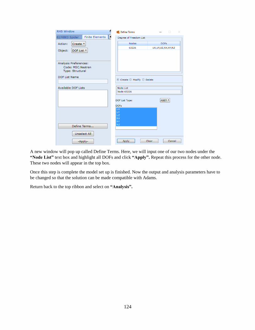
124

A new window will pop up called Define Terms. Here, we will input one of our two nodes under the

“Node List” text box and highlight all DOFs and click “Apply”. Repeat this process for the other node.

These two nodes will appear in the top box.

Once this step is complete the model set up is finished. Now the output and analysis parameters have to

be changed so that the solution can be made compatible with Adams.

Return back to the top ribbon and select on “Analysis”.

125

Under the Analysis tab, click on “Solution Type”. For the output, we will want the normal modes of the

gear. Select “Normal Modes” click on “Solution Parameters”. A new window should pop up. In this

window, click on “ADAMS Preparation”.

126

Once inside of ADAMS Preparation, use the drop down menu to change the Adams Output from None to

“Full Run+ MNF”. The MNF only option is also applicable since this is the file that is required to

integrate into ADAMS however MNF only will not allow for stress calculations. Click on “Units…” to

set the units of the output file to ADAMS. In this case, we will set these units to be millimeters,

kilograms, newtons, seconds. Change the “Num. Shapes to Adams” to “40” Note that this does not set

the units for the part in Patran. If importing flexible bodies into ADAMS causes scale of parts then refer

back to the beginning of the tutorial for import parasolids into Patran. Note that some types of models me

require more mode shapes than others to describe the whole story of the part.

Accept the settings by clicking “OK”, “OK” accept pop up messages window by click “OK”, “OK”

then “OK”, “OK” once more to the Analysis tab.

In the Analysis tab, we will then go to the “Subcases…” menu. Then click “Subcase Parameters…”.

Under Subcase Parameters change the “Number of Desired Roots =” to match the number to ADAMS

output, 40 roots. Once done click “OK”.

127

For stress outputs in ADAMS click on “Output” request and select “Grid Point Stresses” in the Select

Result Type.

128

Click “OK” then “Apply” then “Cancel” to exit out of subcase menu.

Once this is complete the model is ready for analysis. Click “Apply” to run the model. A warning

message will appear, merely click “Yes”.

A command window should pop up indicating that the database has been sent to Nastran for analysis.

Once the analysis is complete the command window will close.

129

Once the window closes, navigate back to the working directory in windows explorer. There should be a

number of files created with the name of the specified job, the one we’re looking for is the .mnf file. This

is the Patran output file required for ADAMS integration.

Copy the .mnf file and the parasolid model into a new directory where the ADAMS model will be

created. This, again, ensures that all associated files for the system will remain together in one folder.

Start up ADAMS view and select the option to create new a “New Model”. Enter a model name, select

“No Gravity”, set the unit system to “MMKS” (these units should be as whatever was set for ADAMS

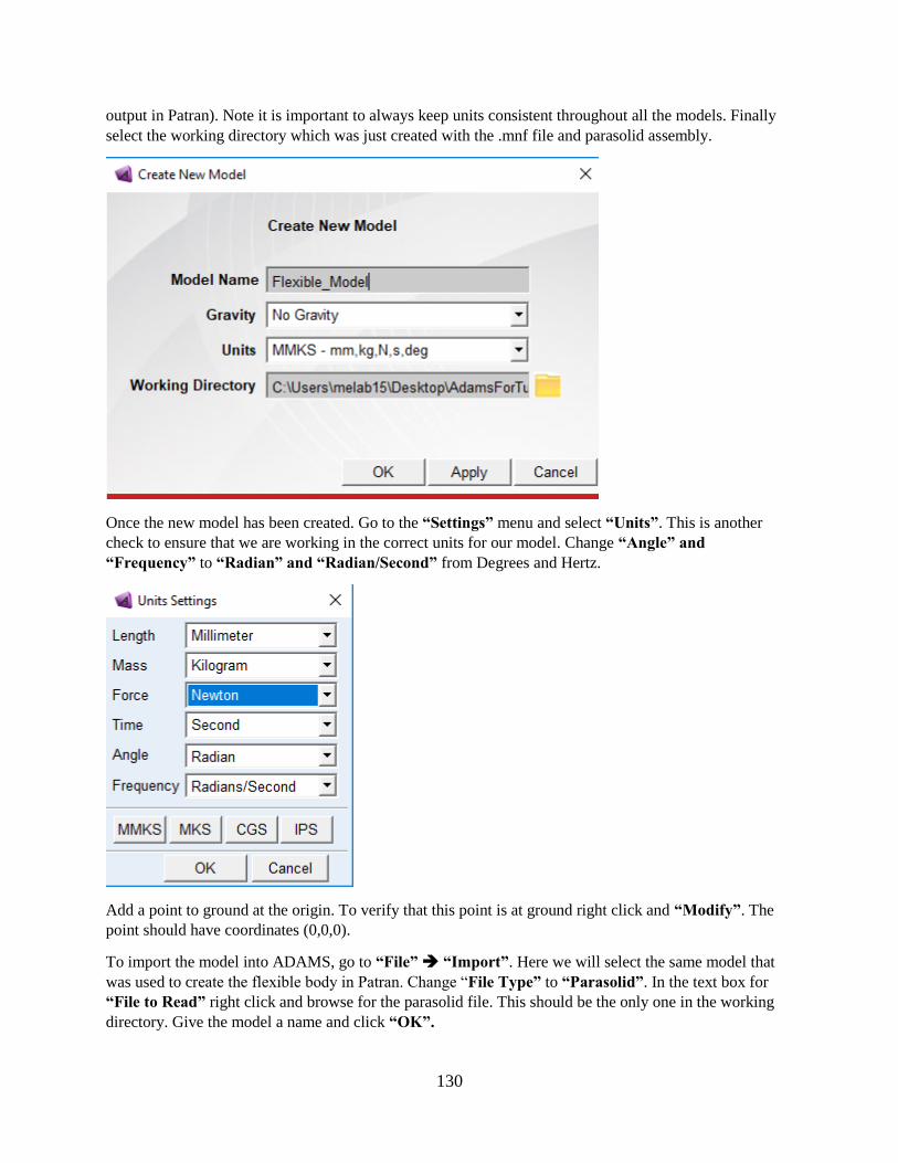
130

output in Patran). Note it is important to always keep units consistent throughout all the models. Finally

select the working directory which was just created with the .mnf file and parasolid assembly.

Once the new model has been created. Go to the “Settings” menu and select “Units”. This is another

check to ensure that we are working in the correct units for our model. Change “Angle” and

“Frequency” to “Radian” and “Radian/Second” from Degrees and Hertz.

Add a point to ground at the origin. To verify that this point is at ground right click and “Modify”. The

point should have coordinates (0,0,0).

To import the model into ADAMS, go to “File” ➔ “Import”. Here we will select the same model that

was used to create the flexible body in Patran. Change “File Type” to “Parasolid”. In the text box for

“File to Read” right click and browse for the parasolid file. This should be the only one in the working

directory. Give the model a name and click “OK”.

131

This will import the full model assembly that was created for all three stages in Solidworks. All the

unnecessary parts can be removed by going to the model tree on the left and deleting them. Give the rest

of the parts a density (7.77E-6 kg/mm^3). Set initial velocity about the z axis to 0 .

The flexible body in this model will be the SunStage1 which we have just put through Patran. To create

flexible model, right click the part on the model tree and click “Make Flexible” and import to import the

mnf file for the gear.

132

A new window will pop up where the mnf file can be imported into ADAMS. Right click on the blank

text box next to the MNF File Drop down menu and click “Browse”. Select the .mnf file desired to use

for analysis in this case there is only one.

There are options at this point to reposition the new flexible model of SunStage2. However, the part will

orient itself in the same location when using the same parasolid model for both ADAMS and Patran. In

these case, nothing needs to be done to reposition the part. Click “OK” to import the flexible part.

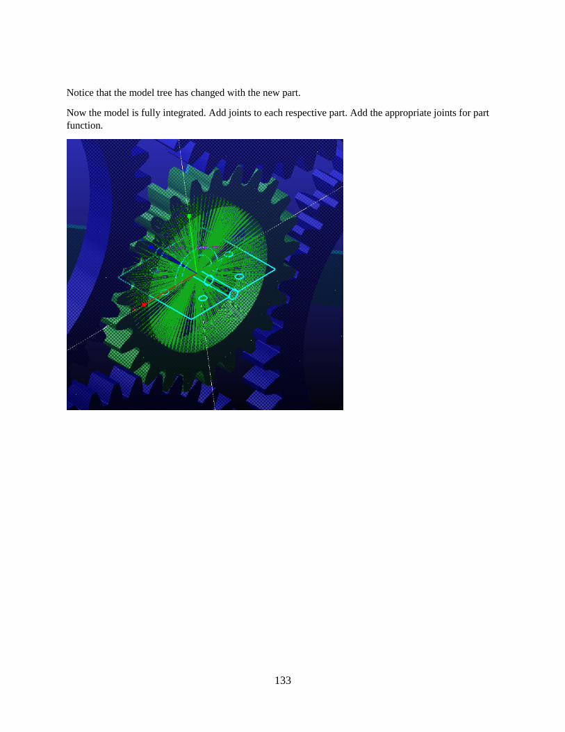
133

Notice that the model tree has changed with the new part.

Now the model is fully integrated. Add joints to each respective part. Add the appropriate joints for part

function.

134

For a simple angular velocity input and

resistive torque. Add motion to the orange

gear by selecting the revolute joint associated

with it and set the type to “Velocity” and

function to “1.76” radians/second. Set initial

velocity about z axis on the flexible body to 0.

Add a resistive torque to the appropriate

torque. To add a contact force between the two

gears. Click on “Create a Contact” in the

Special Forces section at the top ribbon. In the

contact menu, select the Contact Type text box

and change from Solid to Solid to “Flex Body

to Solid”. If this is not set, the flexible body

cannot be selected. This is required to be

specified since ADAMS Solver is capable of

using 2 different codes: FORTRAN and C++.

Fortran is not able to handle contact that is

more than a point to a Plane. This will indicate

that C++ Solver will be used. In the text field

for “I Flexible Body” right click and select

pick and click on the Flexible body. Repeat

this for the J Solid and select the orange output

gear. Specify the Impact model Stiffnes, Force

Exponent, Damping, and Pentration Depth.

135

Once all forces, motion, joints are complete. Run the simulation, wait for it to finish and open the plotting

option. In the main ADAMS window go to the Tools drop down menu and select “Plugin Manager…”.

Check the box to load “ADAMS Durability” and click “OK”. Go back to the plot window, right click

the main plot area and select “Load Animation” at the bottom section select “Contour Plots”. Here

there are options for what type of stress we want to display on the animation and the ability to adjust the

scale for those stress options.

136

This is an example Contour Plot for Max Principal Stress on the Flexible body.

Note that the mesh made for this gear is quite course due to the machines ability to process a large

number of output nodes and a fine mesh on the gear teeth in Patran. This will be a common issue with

gear meshing where a finer mesh on the gear teeth will take large amounts of computer processing power

to run a full analysis.

137

APPENDIX B - VIEW FLEX TUTORIAL

MSC Adams Flexible Body Creation for a Fix Axis Output Gear in

a Planetary Gear System Assembly: A Tutorial

Tananant (Mel) Boonya-ananta

[email protected]

Mechanical Engineering Department

California Polytechnic State University

San Luis Obispo, CA 93407

138

Tutorial.

Prepare a model using Solidworks or similar CAD programs as a Parasolid file (.x_t or .x_b). For this

tutorial a file has been prepared as Stage3NoCrack2.x_t.

Start by opening MSC ADAMS View.

Create a new directory with the parasolid file and choose that as the working directory for ADAMS.

Once the model has been created, navigate File > Import. Select Parasolid in the drop down menu under

File Type. Right click the text box under File To Read and browse for the parasolid file name

Stage3NoCrack.x_t. Assign a name to the model.

The imported model should look like this:

139

Switch from wireframe view to shaded model view:

140

First define the mass properties of each body:

Add a marker to Ground at location (0,0,0). This will provide a good locating feature for joints.

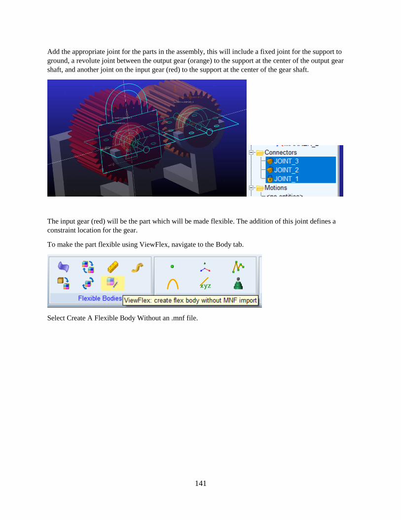
141

Add the appropriate joint for the parts in the assembly, this will include a fixed joint for the support to

ground, a revolute joint between the output gear (orange) to the support at the center of the output gear

shaft, and another joint on the input gear (red) to the support at the center of the gear shaft.

The input gear (red) will be the part which will be made flexible. The addition of this joint defines a

constraint location for the gear.

To make the part flexible using ViewFlex, navigate to the Body tab.

Select Create A Flexible Body Without an .mnf file.

142

This will bring up a menu. Define the mesh properties and the number of Normal Modes required for the

body.

Once the properties are in created, Click OK. Note that this is a coarse mesh. The quality of the mesh is

dependent on the computing power of the computer. Higher end computers will be able to create a fine

mesh due to the available computing power.

Wait for the message window to display to complete. This will create multiple new files as a result of

creating a flexible boy in the working directory.

143

The two main files to be aware of in this directory is the .f06 file and the .mnf file. The .f06 file is the file

that contains any types of error that would come about in the flexible body creation process. This file can

be open in NotePad or NotePad++ and viewed to determine issues in the process. The .mnf file is the

Modal Neutral File which contains the stress analysis information that allows ADAMS to perform the

stress analysis under a dynamic simulation.

The model tree will show that original part as suppressed and hidden and replace it with a new flexible

body as denoted by the rainbow color cube in the left side.

Navigate to the Settings menu and click on Units. Select Radians for Angle.

144

Select the Motions Ribbon and Click on Rotational Joint under Joint Motions

Pick Joint 3 as the joint of interest for the input motion.

Set the motion type to velocity and the function as 110. This sets the input velocity to be 110 rad/sec.

Add contact to the two gears. Navigate to Forces Ribbon and click Contact under Special Forces.

145

In the Create Contact menu. Change the type to be Flex Body to Solid. Select The new flexible body as I

Flexible Body and the second gear (orange) under J Solid.

Uncheck Force Display.

Change the contact stiffness to 5.0E6, leave the force exponent as 2.2, change the damping to 10000,

aAnd Penetration depth to 0.01. Note that all these units contain millimeters as the primary unit of length.

In order to set up the measurement, three markers must be added to the model. One at the origin, another

to create an axis to measure from, and the last to track the rotating point.

First, navigate back to the Bodies Ribbon and select Marker under the Construction section. Add the

marker to Ground and select the origin. Once added, right click the new marker (Marker_10) and click

Info. This will show the coordinates of the marker to make sure that it is one (0,0,0).

146

Rename this Marker to AngleMeas2.

Create another Marker on Ground on the XY Plane that is horizontal at location (-50,0,0) and rename this

to AngleMeas1. Hiding the gear body will make this marker easier to place without accidentally placing it

on a specific node on the gear.

Create another marker on the flexible gear at the same location as AngleMeas1 marker but on the gear

body instead of ground.

147

This marker will sometimes be added slightly shifted from (-50, 0, 0). Right click the marker (Marker_12)

and click Modify. Change the coordinates to (-50, 0, 0). Click OK.

Rename to AngleMeas3.

Navigate to the Design Exploration Ribbon. Under the Measures Section select Create a new Angle

Measurement.

Click on Advanced to get a new popup window. In this window, the three markers that were just created

will be selected to define the angle measurement.

Select AngleMeas1 under First Marker. AngleMeas2 for the Middle Marker. AngleMeas3 for the Last

Marker.

Click OK. A new window will pop up to show the angle measurement over time. Hit escape to exit out of

the angle measurement menu.

148

Move to the Simulation Ribbon and Select Run an Interactive Simulation under the Simulate Section. A

new pop up window will appear with simulation parameters. Set the simulation End Time to 0.057

seconds and use 200 Steps. 0.57 is the amount of time that the Red Gear will complete 1 full rotation.

Click the Green Arrow to Run the simulation. Select Plotting once the simulation has completed.

149

First, plot the angular velocity about the z axis of both the gears to see that it produces the correct ratio.

This is done by selecting Objects for Source, the gear for Object, angular velocity for Characteristic, and z

as the component then Add Curves.

The Plot of these two components should look like this:

The input is the blue curve and the output is the red curve. The input velocity should be 110 rad/sec and

the output should be around 137.5. This is representative of a 1.25 gear ratio.

In order the plot the tooth stress, the nodes must first be identified. To identify the Nodes that stress will

be measured from, under the Durability Menu at the top of the Plot Window select Nodal Plots… (If

Durability is not there, go to Tools > Plugin > Manager and check Adams Durability under Yes in the

Load Column).

A Compute Nodal Plot window will pop up. Under Flexible Body select the Flexible Gear. Then, in the

Node to Add to List text box, right click and click Pick Flexbody Node.

150

Mouse over the desired Node and not down the Node Number.

Copy the Node Number into the Select Node List. Here multiple nodes can be selected to analysis the

stress at different nodes. Once added Click OK.

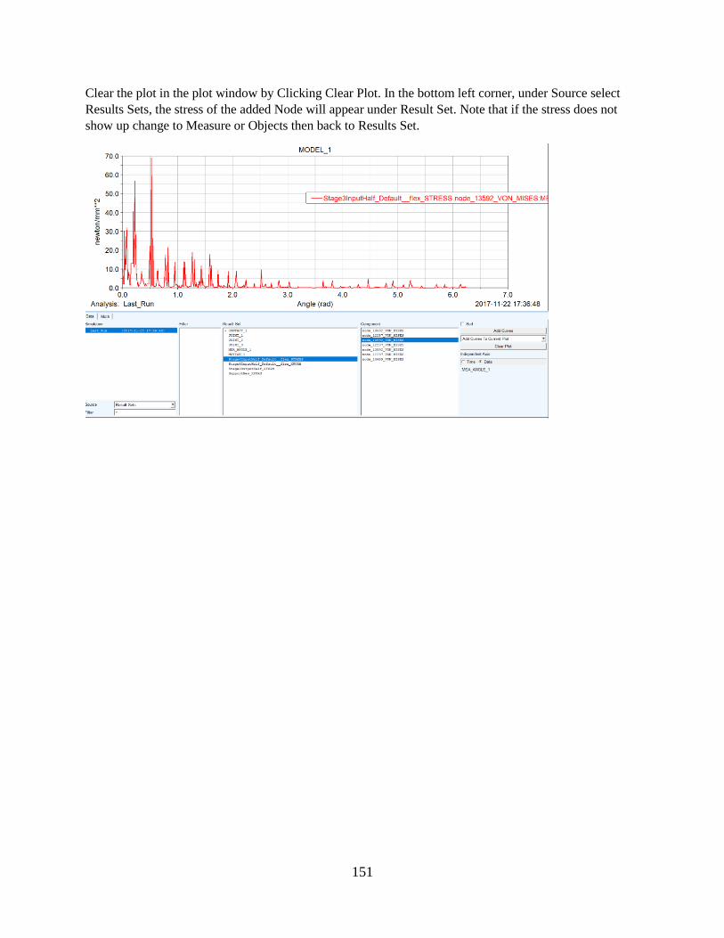
151

Clear the plot in the plot window by Clicking Clear Plot. In the bottom left corner, under Source select

Results Sets, the stress of the added Node will appear under Result Set. Note that if the stress does not

show up change to Measure or Objects then back to Results Set.

Documents

VIBRATION ANALYSIS OF A WIND TURBINE MULTI-STAGE …