Vertical Set Square Distance: A Fast and Scalable Technique to Compute Total Variation in Large Datasets Taufik Abidin, Amal Perera, Masum Serazi, William

Vertical Set Square Distance: Vertical Set Square Distance: A Fast and Scalable Technique to Compute A Fast and Scalable Technique to Compute

Total Variation in Large DatasetsTotal Variation in Large Datasets

Taufik Abidin, Amal Perera, Masum Serazi, William Perrizo

20th International Conference on Computer and Their Applications

March 16-18, 2005

Louisiana, New Orleans

20th International Conference on CATA 2005

Outline:Outline: Introduction

Motivation

Contribution

P-tree Vertical Data Structure

Vertical Set Square Distance (VSSD)

Experimental Results

Conclusion and Future Works


IntroductionIntroduction The determination of closeness (distance) of a point to

another point or to a set of points (average distance) is required in data mining tasks.

For example: Distance-based clustering.

Distance is used to determine in which cluster a certain point should be placed, i.e. K-means.

Near nbr or case-based classification

The assignment of class label to an unclassified point is based on the majority of class label of the nearest neighbor points. “Nearest” here implies the closest distance of points.


One way to measure the distance from a certain point to a set of points is by examining the actual total separation of the set of points from the point in question

However, if the examination is done point by point when the set is very large, scanning the entire space causes the approach to be very costly, slow and non-scalable.

In this paper, we introduce a new technique called the Vertical Set Square Distance (VSSD) that can scalably, quickly and accurately compute the total length of separation (total variation) of a set of points about a point.

Introduction (cont)Introduction (cont)


In data mining, efforts have focused on finding techniques that can scalably deal with large cardinality of dataset due to the explosive growth of data stored in digital form.

Most existing approaches for measuring closeness of points are slow and computationally intensive (often relying upon sampling to become useable).

The availability of P-tree technology (vertical data structure) is an appropriate data structure to solve this curse of cardinality.

MotivationMotivation


We introduce a new vertical technique that scalably, quickly and accurately computes the total length of separation of a set of points about a fixed point.

We present empirical results based on real and synthetic datasets and show the one-to-one comparison in terms of scalability and speed (time) between our new method that uses the vertical approach (P-tree vertical data structure) and other method that uses the horizontal approach (record-based).

Our ContributionsOur Contributions


P-tree vertical data representation consists of set structures essentially representing the data column-by-column rather than row-by-row (i.e. relational data).

The construction of P-trees from an existing relational table is typically by decomposing each attribute in the table into separate bit vectors (e.g., one for each bit position of a numeric attribute or one bitmap for each category in a categorical attribute). The construction for raw data coming from a sensor platform is done directly (without creating a horizontal relational table first.Note that many sensor platforms (e.g.,

RSI sensors), product raw vertical data.

P-Tree Vertical Data StructureP-Tree Vertical Data Structure


The Construction of P-TreeThe Construction of P-Tree

The construction of the P- Tree:

1. Vertically project each attribute.2. Vertically project each bit position.3. Compress each piece of bit slice into a P-tree.

Logical operations are AND (), OR () and complement (').

Root count operation is the count of 1-bits from the resulting P-trees logical operations

0 1 0 1 1 1 1 1 0 0 0 10 1 1 1 1 1 1 1 0 0 0 00 1 0 1 1 0 1 0 1 0 0 10 1 0 1 1 1 1 0 1 1 1 11 0 1 0 1 0 0 0 1 1 0 00 1 0 0 1 0 0 0 1 1 0 11 1 1 0 0 0 0 0 1 1 0 01 1 1 0 0 0 0 0 1 1 0 0

R11 R12 R13 R21 R22 R23 R31 R32 R33 R41 R42 R43

P11 P12 P13 P21 P22 P23 P31 P32 P33 P41 P42 P43 0 0 0 0 1 10

0 1 0 0 1 01

0 0 00 0 0 1 01 10

0 1 0

0 1 0 1 0

0 0 01 0 01

0 1 0

0 0 0 1 0

0 0 10 1

0 0 10 1 01

0 0 00 1 01

0 0 0 0 1 0 010 01^ ^ ^ ^ ^ ^ ^ ^ ^

010 111 110 001011 111 110 000010 110 101 001010 111 101 111101 010 001 100010 010 001 101111 000 001 100111 000 001 100

=

R[A1] R[A2] R[A3] R[A4] 010 111 110 001011 111 110 000010 110 101 001010 111 101 111101 010 001 100010 010 001 101111 000 001 100111 000 001 100

R(A1 A2 A3 A4)2 7 6 16 7 6 02 7 5 12 7 5 75 2 1 42 2 1 57 0 1 47 0 1 4


Binary Representation

Let x be a numerical domain of attribute Ai of relation R(A1, A2, …, Ad), then x written in b bits binary number is shown in the left-hand side term of the equation below.

The first subscript of x is the index of the attribute to which x belong. The second subscript of x indicates the bit position. The summation on the right-hand side of the equation is equal to the actual value of x as a decimal number.

Vertical Set Square DistanceVertical Set Square Distance

0

1,0,1, 2

bjji

jibi xxx


Let X be a set of vectors in a relation R(A1, A2, …, Ad), let

PX be the P-tree class mask of X, x is a vector : and a is a target vector (also in d-dimensional space), then the vectors x and a in binary can be written as:

The total variation of a set of vectors in X about a vector a can be computed vertically using Vertical Set Square Distance (VSSD) defined as follows:

Vertical Set Square Dist. (Cont)Vertical Set Square Dist. (Cont)

Xx

),,,( 0,)1(,0,2)1(,20,1)1(,1 dbdbb xxxxxxx ),,,( 0,)1(,0,2)1(,20,1)1(,1 dbdbb aaaaaaa



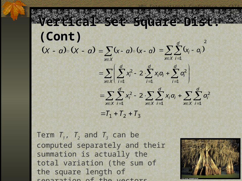
aXaX axaxXx

2

1

Xx

d

iii ax

Xx

d

i

d

iiii

d

ii aaxx

1 1

2

1

2 2

Xx Xx

d

i Xx

d

iiii

d

ii aaxx

1 1

2

1

2 2

321 TTT

Term T1, T2 and T3 can be computed

separately and their summation is actually the total variation (the sum of the square length of separation of the vectors connecting X and a.



Xx

d

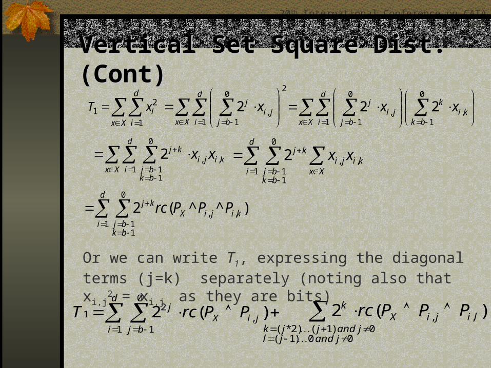
iixT

1

21

d

i bjjiX

j PPrcT1

0

1,

21 )(2 )(2

0 0)1(0 )1()2*(

,,

jandjl

jandjjklijiX

k PPPrc

2

1

0

1,2

Xx

d

i bjji

j x

0

1,

1

0

1, 22

bkki

k

Xx

d

i bjji

j xx

Xx

d

ibkbj

kijikj xx

1

0

11

,,2

Xx

kiji

d

ibkbj

kj xx ,,1

0

11

2

)^^(2 ,,1

0

11

kijiX

d

ibkbj

kj PPPrc

Or we can write T1, expressing the diagonal terms (j=k) separately (noting also that xi,j

2 = xi,j as they are bits)



Xx

d

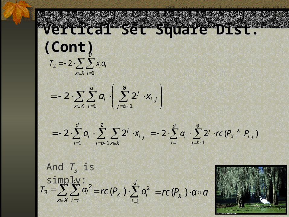
iiiaxT

12 2

Xx

d

i bjji

ji xa

1

0

1,22

d

i bj Xxji

ji xa

1

0

1,22

d

i bjjiX

ji PPrca

1

0

1, )(22

Xx

d

iiiaT 2

3

d

iiX aPrc

1

2)(

And T3 is simply:

aaPrc X )(



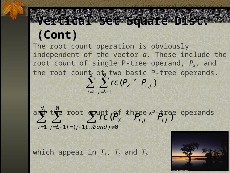
The root count operation is obviously independent of the vector a. These include the root count of single P-tree operand, PX, and the root count of two basic P-tree operands.

and the root count of three P-tree operands

which appear in T1, T2 and T3.

d

i bjjiX PPrc

1

0

1, )(

d

i bj jandjllijiX PPPrc

1

0

1 0 0)1(,, )(



The independency allows us to pre-compute the root counts once in advance, during the construction of the P-tree, and can use them repeatedly as needed, regardless of the number of target vectors a.

This amortizes the cost of P-tree ANDing for high value datasets, e.g. cancer analysis, RSI, etc.


Horizontal Set Square DistanceHorizontal Set Square Distance(HSSD) as a comparison method(HSSD) as a comparison method

Let X, a set of vectors in R(A1,A2 … Ad) and

x = (x1, x2, …, xd) is a vector belong to X and

a = (a1, a2, …, ad) is a target vector

Then the horizontal set square distance (HSSD) is defined as follows:

2

1

Xx

d

iii

Xx

axaxaxaXaX


Experimental ResultsExperimental Results The experiments were conducted using both real and

synthetic datasets.

The goals are to compare the execution time (speed) and scalability of our algorithm employing a vertical approach (vertical data structure and horizontal bitwise AND operation) with a horizontal approach (horizontal data structure and vertical scan operation).

Performance of both algorithms was observed under different machine specifications, including an SGI Altix machine.


Experimental Results (Cont.)Experimental Results (Cont.)

The specification of machines used in the experiments.

Machine Specification

AMD1GB AMD Athlon K7 1.4GHz, 1GB RAM

P42GB Intel P4 2.4GHz processor, 2GB RAM

SGI AltixSGI Altix CC-NUMA 12 processor shared memory (12 x 4 GB RAM)


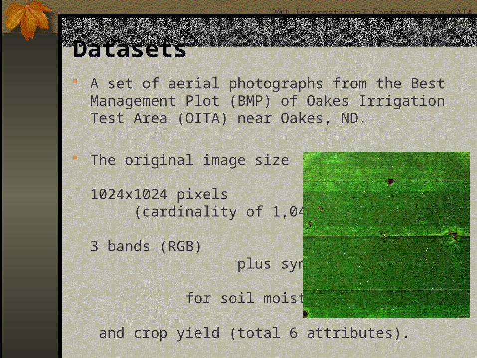
DatasetsDatasets A set of aerial photographs from the Best Management

Plot (BMP) of Oakes Irrigation Test Area (OITA) near Oakes, ND.

The original image size (dataset) is 1024x1024 pixels (cardinality of 1,048,576), contains 3 bands (RGB) plus synchronized data for soil moisture, soil nitrate and crop yield (total 6 attributes).


Datasets (Cont.)Datasets (Cont.) The datasets contain 4 different yield classes:

Low Yield ( 0 < intensity <= 63) Medium Low Yield ( 63 < intensity <= 127) Medium High Yield (127< intensity <= 191) High Yield (191< intensity <= 255)

With super sampling five synthetic datasets are created: 2,097,152 rows 4,194,304 rows (2048x2048 pixels) 8,388,608 rows 16,777,216 rows (4096x4096 pixels) 25,160,256 rows (5016x5016 pixels)


Timing and Scalability ResultsTiming and Scalability ResultsObservation 1. The first performance evaluation was done on a P4 2 GB

RAM machine using synthetic datasets having 4.1 and 8.3 million data tuples.

We use 100 arbitrary unclassified target vectors (resulting

in 400 classification computations as to predicted yeild).

Datasets of sizes greater than 8.3 million rows cannot be executed in this machine due to out of memory problems when running Horizontal Set Square Distance (HSSD).


ResultsResults VSSD vs HSSD Time Comparison Using 100 Test Cases on 4,194,304 Rows Dataset

-1

1

3

5

7

9

0 10 20 30 40 50 60 70 80 90 100

Test Case ID

Tim

e(i

n S

econ

ds)

VSSD HSSDVSSD vs HSSD Time Comparison

Using 100 Test Cases on 8,388,608 Rows Dataset

-1

1

3

5

7

9

11

13

15

17

0 10 20 30 40 50 60 70 80 90 100Test Case ID

Tim

e(i

n S

econ

ds)

VSSD HSSD

Dataset size

(# of Rows)

Average Time to Compute Total Variation for Each Test Case in (Seconds)

VSSD HSSD

4,193,304 0.0003 7.3800

8,388,608 0.0004 15.1600


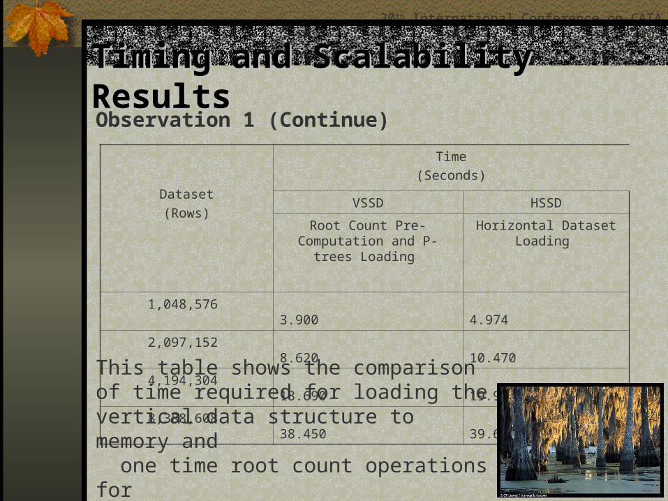
Timing and Scalability ResultsTiming and Scalability ResultsObservation 1 (Continue)

Dataset

(Rows)

Time

(Seconds)

VSSD HSSD

Root Count Pre-Computation and P-trees Loading

Horizontal Dataset Loading

1,048,576 3.900 4.974

2,097,152 8.620 10.470

4,194,304 18.690 19.914

8,388,608 38.450 39.646This table shows the comparison of time required for loading the vertical data structure to memory and one time root count operations for VSSD, and loading horizontal records to memory needed for HSSD.


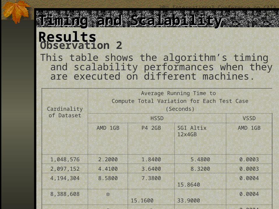
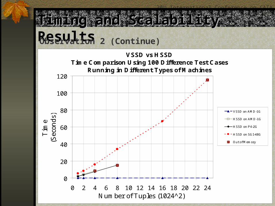
Timing and Scalability ResultsTiming and Scalability ResultsObservation 2This table shows the algorithm’s timing and

scalability performances when they are executed on different machines.

Cardinality of Dataset

Average Running Time to

Compute Total Variation for Each Test Case

(Seconds)

HSSD VSSD

AMD 1GB P4 2GB SGI Altix 12x4GB AMD 1GB

1,048,576 2.2000 1.8400 5.4800 0.0003

2,097,152 4.4100 3.6400 8.3200 0.0003

4,194,304 8.5800 7.3800 15.8640 0.0004

8,388,608 15.1600 33.9000 0.0004

16,777,216 66.5400 0.0004

25,160,256 115.2040 0.0004


Timing and Scalability ResultsTiming and Scalability ResultsObservation 2 (Continue)

VSSD vs HSSD Time Comparison Using 100 Difference Test Cases

Running in Different Types of Machines

0

20

40

60

80

100

120

0 2 4 6 8 10 12 14 16 18 20 22 24Number of Tuples (1024 2̂)

Tim

e(S

econ

ds)

VSSD on AMD-1G

HSSD on AMD-1G

HSSD on P4-2G

HSSD on SGI -48G

Out of Memory


ConclusionConclusion Vertical Set Square Distance (VSSD) is fast and accurate

way to compute total variation for classification, clustering and rule mining, and scale well to very large datasets compare to the traditional horizontal approach (HSSD).

The complexity of the VSSD is O(d * b2) where d is the number of dimensions and b is the maximum bit-width of the attributes (depends on the width of the data set only).

The VSSD is very fast because of the independency of root counts of P-tree operands to target vector a which allows the pre-computation of counts once in advance, during the construction of the P-tree.


Future WorkFuture Work

Comprehensive study on the Vertical Set Square Distance (VSSD) in many data mining tasks, i.e. classification, clustering or outlier detection.

For classification using VSSD in the voting phase has already been shown to greatly accelerate the assignment of class since the calculation of class votes can be done entirely in one computation without having to visit each individual point, as is the case of the horizontal-based approach.


Thank You…Thank You…

Documents

Vertical Set Square Distance: A Fast and Scalable Technique to Compute Total Variation in Large Datasets Taufik Abidin, Amal Perera, Masum Serazi, William