1

 Vehicle routing using remote asset monitoring: a case

study with Oxfam

Fraser McLeod, Tom Cherrett (Transport)

Güneş Erdoğan, Tolga Bektas (Management)

OR54, Edinburgh, 4-6 Sept 2012

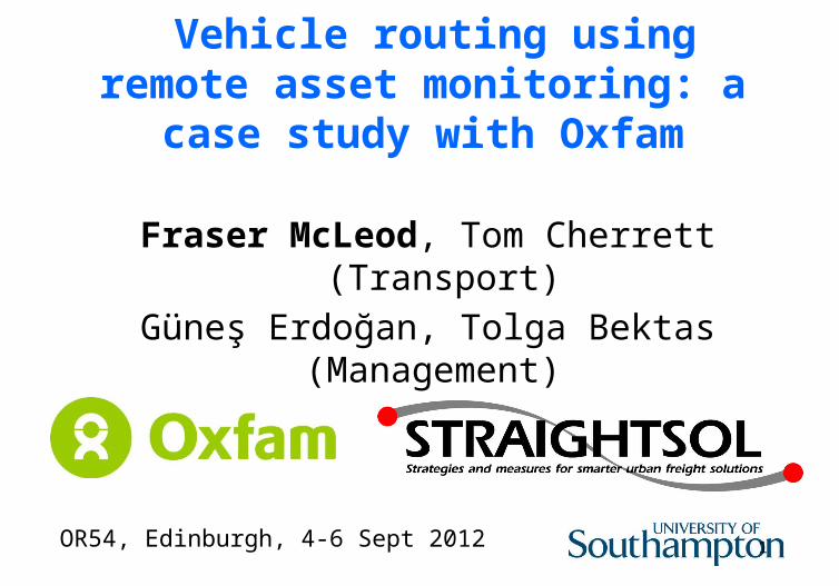
Background

www.oxfam.org.uk/shop

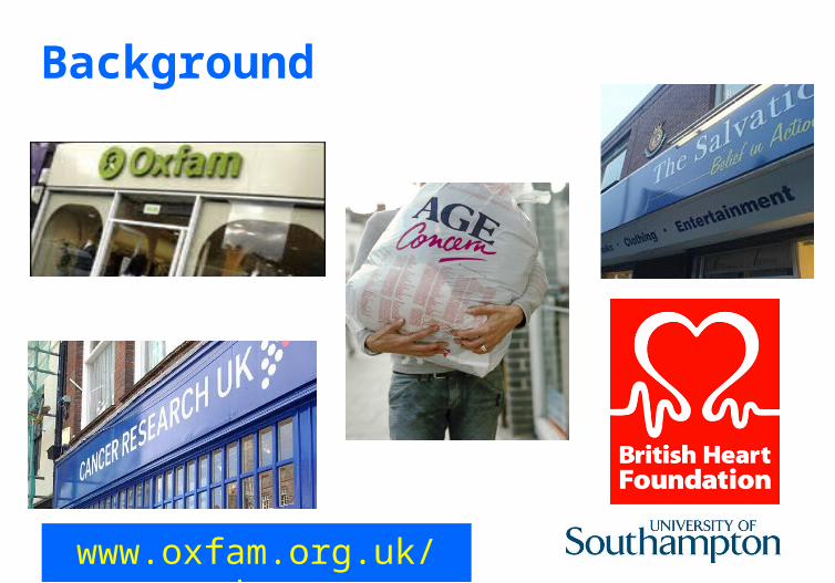
Donation banks

Oxfam bank sites in England

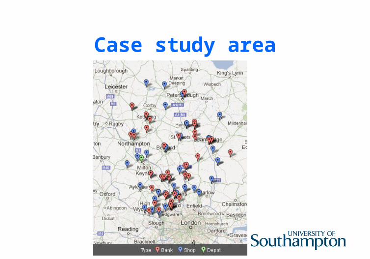
4

Case study area

5

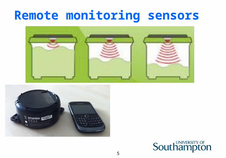
Remote monitoring sensors

6

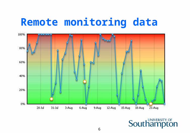
Remote monitoring data

7

Problem summary (requirements)

• Visit shops on fixed days• Visit banks before they become full• Routes required Monday to Friday each

week• Start/end vehicle depot• Single trips each day (i.e. no drop-offs)

8

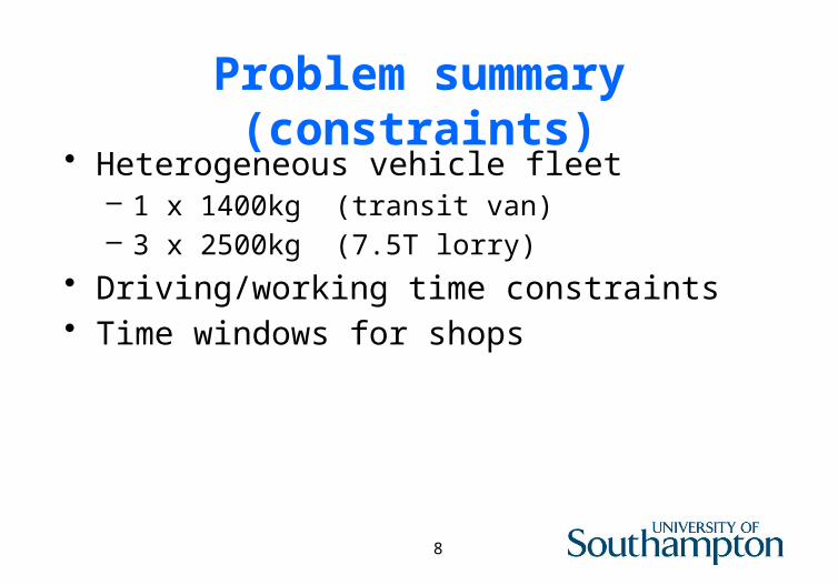
Problem summary (constraints)

• Heterogeneous vehicle fleet– 1 x 1400kg (transit van)– 3 x 2500kg (7.5T lorry)

• Driving/working time constraints• Time windows for shops

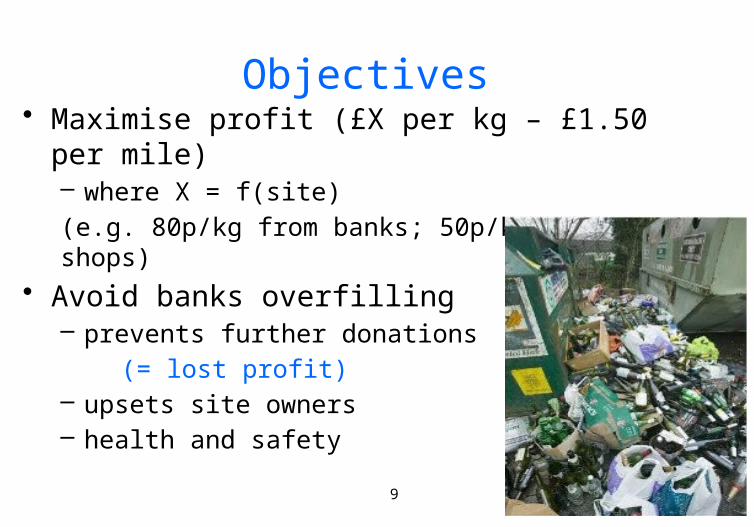
Objectives• Maximise profit (£X per kg – £1.50 per

mile)– where X = f(site) (e.g. 80p/kg from banks; 50p/kg from shops)

• Avoid banks overfilling– prevents further donations (= lost profit)– upsets site owners– health and safety

9

10

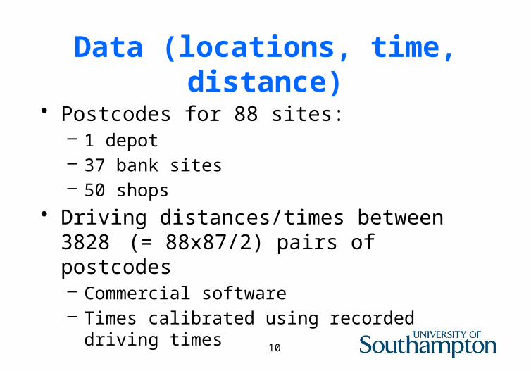
Data (locations, time, distance)

• Postcodes for 88 sites:– 1 depot– 37 bank sites– 50 shops

• Driving distances/times between 3828 (= 88x87/2) pairs of postcodes– Commercial software– Times calibrated using recorded driving

times

11

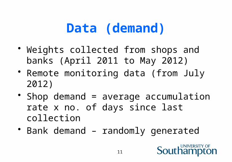
Data (demand)

• Weights collected from shops and banks (April 2011 to May 2012)

• Remote monitoring data (from July 2012)

• Shop demand = average accumulation rate x no. of days since last collection

• Bank demand – randomly generated

12

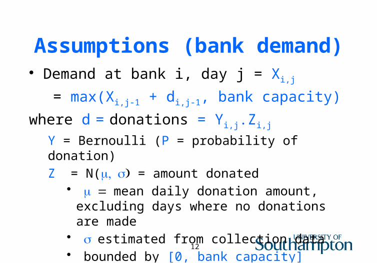
Assumptions (bank demand)

• Demand at bank i, day j = Xi,j

= max(Xi,j-1 + di,j-1, bank capacity)

where d = donations = Yi,j.Zi,j

Y = Bernoulli (P = probability of donation)Z = N( , m s) = amount donated

• m = mean daily donation amount, excluding days where no donations are made

• s estimated from collection data• bounded by [0, bank capacity]

13

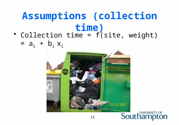
Assumptions (collection time)

• Collection time = f(site, weight) = ai + bi

xi

14

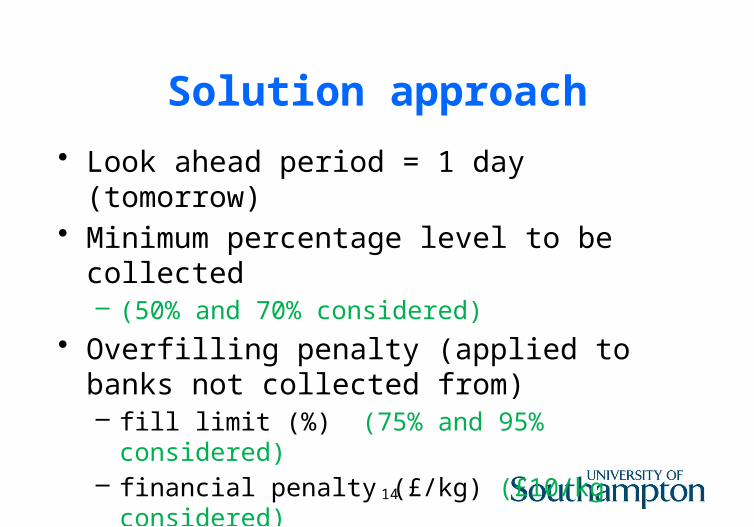
Solution approach

• Look ahead period = 1 day (tomorrow)• Minimum percentage level to be

collected– (50% and 70% considered)

• Overfilling penalty (applied to banks not collected from)– fill limit (%) (75% and 95% considered)– financial penalty (£/kg) (£10/kg considered)

15

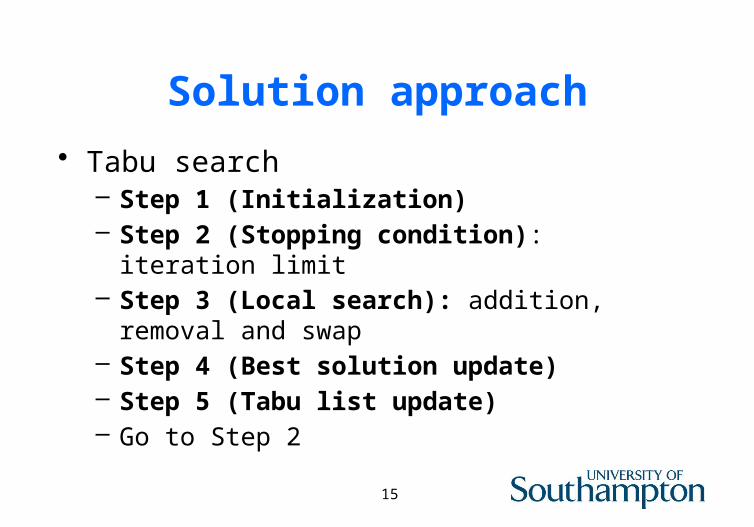
Solution approach

• Tabu search – Step 1 (Initialization) – Step 2 (Stopping condition): iteration

limit– Step 3 (Local search): addition, removal

and swap – Step 4 (Best solution update)– Step 5 (Tabu list update)– Go to Step 2

16

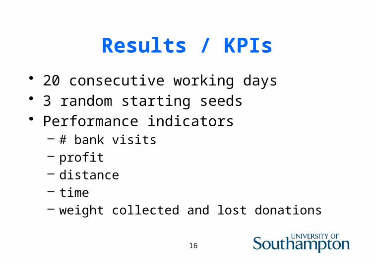
Results / KPIs

• 20 consecutive working days • 3 random starting seeds• Performance indicators

– # bank visits– profit– distance– time– weight collected and lost donations

17

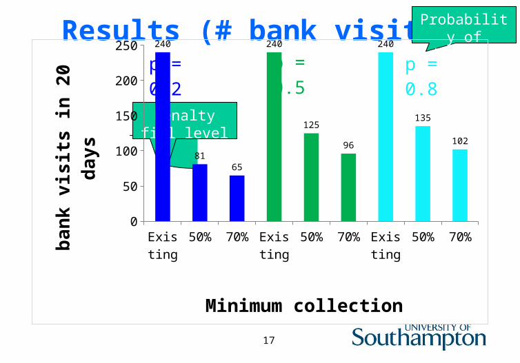
Results (# bank visits)Probability of donation

Penalty fill level

Exist-ing

50% 70% Exist-ing

50% 70% Exist-ing

50% 70%0

50

100

150

200

250 240

8165

240

125

96

240

135

102

Minimum collection

bank

vis

its in

20

days

p = 0.8p = 0.5p = 0.2

18

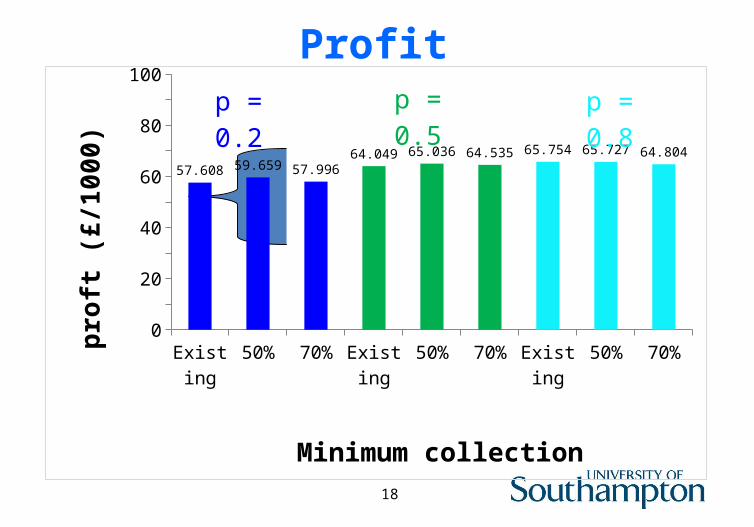
Profit

Exist-ing

50% 70% Exist-ing

50% 70% Exist-ing

50% 70%0

10

20

30

40

50

60

70

80

90

100

57.608 59.659 57.99664.049 65.036 64.535 65.754 65.727 64.804

Minimum collection

proft

(£/1

000)

p = 0.8p = 0.5p = 0.2

19

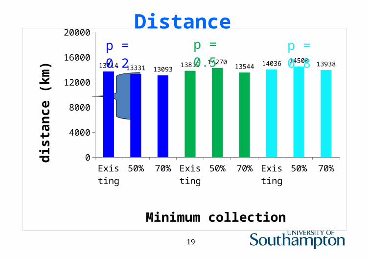
Distance

Exist-ing

50% 70% Exist-ing

50% 70% Exist-ing

50% 70%0

4000

8000

12000

16000

20000

13714 13331 1309313819 14270

13544 14036 1450013938

Minimum collection

dist

ance

(km

)p = 0.8p = 0.5p = 0.2

20

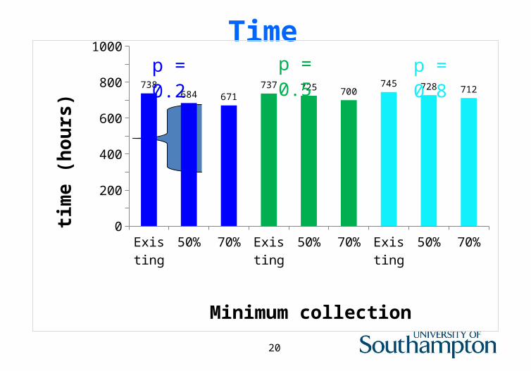
Time

Exist-ing

50% 70% Exist-ing

50% 70% Exist-ing

50% 70%0

100

200

300

400

500

600

700

800

900

1000

738684 671

737 725 700745 728 712

Minimum collection

time

(hou

rs)

p = 0.8p = 0.5p = 0.2

21

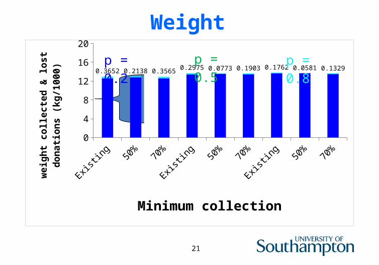
Weight

Existing 50% 70% Existing 50% 70% Existing 50% 70%0

4

8

12

16

20

0.3652 0.2138 0.35650.2975 0.0773 0.1903 0.1762 0.0581 0.1329

Minimum collection

wei

ght c

olle

cted

& lo

st d

onati

ons

(kg/

1000

)p = 0.8p = 0.5p = 0.2

22

Conclusions & Discussion

• Bank visits could be substantially reduced

• But benefits are limited by the requirement to keep shop collections fixed

• Can we improve our modelling approach?