Embed Size (px)
Citation preview
Variational Methods for Time–DependentWave Propagation Problems
Patrick Joly
INRIA Rocquencourt, BP105 Le Chesnay, France ([email protected])
1 Introduction
There is an important need for numerical methods for time dependent wavepropagation problems and their many applications, for example in acous-tics, electromagnetics and geophysics. Although very old, finite differencetime domain methods (FDTD methods in the electromagnetics literature)remain very popular and are widely used in wave propagation simulations,and more generally for the resolution of linear hyperbolic systems, amongwhich Maxwell’s system is a typical example. These methods allow us to getdiscrete equations whose unknowns are generally field values at the points ofa regular mesh with spatial step h and time step ∆t.
For Maxwell’s equations, the Yee scheme [65, 67] is an important andmuch-used example of such a scheme. In 1D, it concerns the following system:
∂u
∂t+ c
∂v
∂x= 0,
∂v
∂t+ c
∂u
∂x= 0, x ∈ R, t > 0 . (1)
Without any mesh refinement, the equations of the scheme are (with standardnotation un
j ≈ u(jh, n∆t))
un+1j − un
j
∆t+ c
vn+1/2j+1/2 − v
n+1/2j−1/2
h= 0,
vn+1/2j+1/2 − v
n−1/2j+1/2
∆t+ c
unj+1 − un
j
h= 0,
(2)where the discrete unknowns are evaluated on a staggered uniform grid. Thereare several reasons that explain the success of Yee type schemes, among whichtheir easy implementation, their efficiency, their accuracy and the fact thata lot of properties of continuous Maxwell’s equations (energy conservation,divergence free property etc.) are respected at the discrete level. In particular,the good performance of Yee’s scheme is related to the following properties:– A uniform regular grid is used for the space discretization, so that there
is a minimum of information to store and the data to be computed arestructured. In other words, one avoids all the complications due to the useof non uniform meshes.
– An explicit time discretization is applied – no linear system has to be solvedat each time step.
2 Patrick Joly
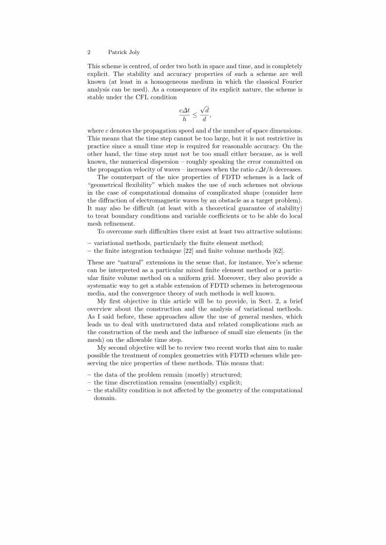
This scheme is centred, of order two both in space and time, and is completelyexplicit. The stability and accuracy properties of such a scheme are wellknown (at least in a homogeneous medium in which the classical Fourieranalysis can be used). As a consequence of its explicit nature, the scheme isstable under the CFL condition
c∆t
h≤
√d
d,
where c denotes the propagation speed and d the number of space dimensions.This means that the time step cannot be too large, but it is not restrictive inpractice since a small time step is required for reasonable accuracy. On theother hand, the time step must not be too small either because, as is wellknown, the numerical dispersion – roughly speaking the error committed onthe propagation velocity of waves – increases when the ratio c∆t/h decreases.
The counterpart of the nice properties of FDTD schemes is a lack of“geometrical flexibility” which makes the use of such schemes not obviousin the case of computational domains of complicated shape (consider herethe diffraction of electromagnetic waves by an obstacle as a target problem).It may also be difficult (at least with a theoretical guarantee of stability)to treat boundary conditions and variable coefficients or to be able do localmesh refinement.
To overcome such difficulties there exist at least two attractive solutions:
– variational methods, particularly the finite element method;– the finite integration technique [22] and finite volume methods [62].
These are “natural” extensions in the sense that, for instance, Yee’s schemecan be interpreted as a particular mixed finite element method or a partic-ular finite volume method on a uniform grid. Moreover, they also provide asystematic way to get a stable extension of FDTD schemes in heterogeneousmedia, and the convergence theory of such methods is well known.
My first objective in this article will be to provide, in Sect. 2, a briefoverview about the construction and the analysis of variational methods.As I said before, these approaches allow the use of general meshes, whichleads us to deal with unstructured data and related complications such asthe construction of the mesh and the influence of small size elements (in themesh) on the allowable time step.
My second objective will be to review two recent works that aim to makepossible the treatment of complex geometries with FDTD schemes while pre-serving the nice properties of these methods. This means that:
– the data of the problem remain (mostly) structured;– the time discretization remains (essentially) explicit;– the stability condition is not affected by the geometry of the computational
domain.
Variational Methods for Time–Dependent Wave Propagation Problems 3
The first approach, that I will describe in Sect. 3, is the fictitious domainmethod. Let us consider the model problem of the scattering of an incidentelectromagnetic wave by a perfectly conducting obstacle. The idea of themethod consists of artificially extending the solution inside the obstacle –which makes possible the use of a uniform, regular 3D grid for the electro-magnetic field – and to introduce at the same time a conforming surfacemesh for the boundary of the obstacle to handle the boundary condition.On this mesh, one computes an auxiliary unknown that can be interpretedas a Lagrange multiplier associated with the boundary condition and coin-cides, in this case, with the surface electric current. The challenge is thento make these two “independent” meshes communicate in a clever way. Thiscan be done through the use of a mixed variational formulation in whichthe boundary condition is taken into account in a weak sense. The stabilityof the method in ensured through a discrete energy conservation. The onlyadditional computational cost (with respect to the standard FDTD scheme)is restricted to the boundary mesh: a sparse positive definite linear systemhas to be solved at each time step.
An alternative approach (that can be combined with the fictitious domainmethod) consists of refining the mesh in the neighbourhood of the obstacle.I will present in Sect. 4 some recent research about conservative space-timemesh refinement methods. When one works with regular grids, the transitionbetween a coarse and a fine grid is necessarily “non conforming”. Moreover,for efficiency and accuracy considerations, one would like to use a local timestep in order to keep the time step/space step ratio constant. Traditional in-terpolation methods can lead to non standard instability phenomena. Here,we shall propose two alternative methods based on the reformulation of theproblem as an artificial domain decomposition. The key issue of these meth-ods is that their stability is guaranteed from the theoretical point of viewthrough the conservation of an appropriate discrete energy. The first methodinvolves the introduction of a Lagrange multiplier on the coarse–fine grid in-terface (as in the so-called mortar element method), while the second doesnot. As in the fictitious domain method, both methods require the solutionof a small, sparse, positive definite linear system on the interface. We shallalso show how spurious numerical phenomena due to a change of grid can beanalysed and controlled.
2 Basic Principles of Variational Methods
In this section, we present a brief introduction (a crash course) to variationalnumerical schemes for time dependent wave propagation models. Almost allthe material contained in this section is very classical, but useful for the nextsections. We do not pretend here to be exhaustive and completely rigorous.That is why all the assumptions needed for a rigorous development will notalways be written and the proofs of a lot of statements will be only sketched
4 Patrick Joly
or omitted when they are trivial. We only wish to present the main ideasof results with a sufficient degree of abstraction and generality in order toemphasise the interest of the approach.
2.1 Mathematical Models
Most of basic wave propagation mathematical models can be rewritten in oneof the two following forms (abstract wave equations):
– As a first order system in time:∂u
∂t− Bv = 0,
∂v
∂t+ B∗u = 0,
(3)
where the unknowns u and v are functions from Ω ⊂ RN (the domain ofpropagation) into Rp and Rq respectively. The two operators B and B∗
are spatial differential operators which are, at least formally, adjoint forappropriate weighted inner products (u, u)P – with norm ‖u‖P – in L2(Ω)p
and (v, vD) – with norm ‖v‖D – in L2(Ω)q. In the applications, verifyingsuch a property amounts in practice to applying an adequate integrationby parts formula.
– As a second order system in time, either after elimination of v or u:
∂2u
∂t2+ Au = 0 ; (4)
∂2v
∂t2+ Av = 0 . (5)
Both operators A = BB∗ and A = B∗B are formally positive self-adjoint(in some weighted L2 space). By convention, we shall call u the primalvariable and v the dual one. Accordingly, we shall refer to problem (4) asthe primal problem and to problem (5) as the dual one. In the same way‖.‖P is the primal L2 norm and ‖.‖D the dual one.
Of course, the mathematical model has to be completed by initial and bound-ary conditions (which play a role in the adjointness results etc.). We shall omitthem for simplicity in this introductory section.
Let us give several concrete examples for illustration:
– The 1D wave equation:B =
∂
∂x, B∗ = − ∂
∂x, A = − ∂2
∂x2,
(u, u)P =∫
Ω
u u dx , (v, v)D =∫
Ω
v v dx .(6)
Variational Methods for Time–Dependent Wave Propagation Problems 5
– The acoustic wave equation:u = p ∈ R1 (the pressure field) , v ∈ R3 (the velocity field) ,
B = K div , B∗ = − ρ−1∇, A = − K div (ρ−1∇),
(p, p)P =∫
Ω
K−1 p p dx , (v, v)D =∫
Ω
ρ−1 v · v dx ,
(7)
where ρ is the density of the fluid and K denotes its Lame constant.– Maxwell’s equations:
u = e ∈ R3 (the electric field), v = h ∈ R3 (the magnetic field),
B = ε−1 curl, B∗ = µ−1 curl, A = − ε−1 curl (µ−1curl),
(e, e)P =∫
Ω
ε e · e dx , (h, h)D =∫
Ω
µ h · h dx ,
(8)
where ε and µ are respectively the dielectric permittivity and the magneticpermeability.
– Elastodynamics equations:u = v ∈ R3 (velocity field) , v = σ ∈ R6 ((symmetric) stress tensor)
B = ρ−1 div , B∗ = − Cε(·), A = −ρ−1 div C(ε(·)),
(v, v)P =∫
Ω
ρ v · v dx , (σ, σ)D =∫
Ω
C−1 σ · σ dx ,
(9)where ρ denotes the density, C the operator appearing in Hooke’s law andwhere the (tensor valued) differential operator ε(·) is defined by:
εij(v) =12(∂vi
∂xj+
∂vj
∂xi).
A fundamental property of such models is that they are intrinsically linkedto the conservation in time of an energy:
E(t) =12
(‖u(t)‖2
P + ‖v(t)‖2D
)for model (3) and
E(t) =12
( ∣∣∣∣∣∣∣∣∂u
∂t(t)
∣∣∣∣∣∣∣∣2P
+ (Au(t), u(t))P
)
for model (4). These energies make sense once the functional framework hasbeen rigorously prescribed and have a physical meaning in each of the con-crete examples evoked above.
6 Patrick Joly
Remark 1. The models we have considered correspond to the propagation ofwaves in the absence of sources. The presence of source terms would implythe addition of right hand sides in the equations and the conservation of theenergy would be replaced by an energy identity relating the variation of theenergy to the source term.
2.2 Variational Formulations
The variational formulation in space of the above problems is a rigorousreformulation in which the unknown is sought as a function of time withvalues in spaces of functions of the space variable x. We therefore need tointroduce a functional framework. In this way, one separates the role of thespace and time variables, which naturally leads to different discretizationprocedures in space and time.
Remark 2. In what follows, we shall systematically omit the role of the bound-ary conditions in such a way that all that follows in this section is rigorouslyvalid only in the case Ω = RN . In the other cases, the boundary conditionshave a role in the integration by parts and may influence the definition of thefunctional spaces. However, what is important for our purpose is the abstractform of the problem ((12), (15) or (16)) that we shall obtain. This remainsvalid for a number of physically relevant boundary conditions, and is onlyslightly different for some other ones.
Second Order Problems Let us first present the variational formulationof problem (4). Formally, it is equivalent to take the L2 scalar product ofequation (4) with a test function u that only depends on the space variable(i.e. multiply (4) by u and integrate over Ω). To justify this, we need tointroduce a functional framework. Let H(B∗) be the Hilbert space:
H(B∗) = u ∈ L2(Ω)p / B∗u ∈ L2(Ω)q, (10)
equipped with the norm
‖u‖2H(B∗) = ‖u‖2
P + ‖B∗u‖2D. (11)
Then the variational formulation of (4) can be written as follows:Find u(t) : R+ −→ U = H(B∗) such that:d2
dt2(u(t), u)P + a(u(t), u) = 0, ∀ u ∈ U,
a(u, u) = (B∗u,B∗u)D, ∀ (u, u) ∈ U × U.
(12)
This is also the appropriate formulation for defining the notion of weak so-lutions to the evolution problem and developing the corresponding existencetheory (see for instance [53]). Note that the bilinear form a(·, ·) is positiveand symmetric (which is intimately related to the energy conservation). Asan illustration (again neglecting the boundary conditions etc.):
Variational Methods for Time–Dependent Wave Propagation Problems 7
– For example (7): U = H1(Ω) and a(p, p) =∫
Ωρ−1 ∇p · ∇p dx.
– For example (8) : U = H(curl, Ω) and a(e, e) =∫
Ωµ curl e · curl e dx.
– For example (9) : U = H1(Ω)3 and a(v, v) =∫
ΩC ε(v) · ε(v) dx.
Indeed, we have an analogous variational formulation for the dual problem(5), which leads to working in the Hilbert space:
H(B) = v ∈ L2(Ω)q / Bv ∈ L2(Ω)p, (13)
equipped with the norm
‖v‖2H(B) = ‖v‖2
D + ‖Bv‖2P . (14)
First Order Problems For these problems, the appropriate variationalformulation is the so-called mixed variational formulation (see [16] for sta-tionary problems). Once again the principle is to multiply the two equationsof system (3) by test functions and to integrate over Ω, but the key pointthis time is to apply integration by parts only for one of the two equations.
– The primal-dual formulation. This formulation holds in a functionalframework in which the regularity is put on the primal variable u. Moreprecisely, u will be sought in the space U = H(B∗) and v in the spaceV = L2(Ω)q:
Find (u(t), v(t)) : R+ −→ U × V such that:ddt
(u(t), u)P − b(u, v(t)) = 0, ∀ u ∈ U,
ddt
(v(t), v)D + b(u(t), v) = 0, ∀ v ∈ V,
b(u, v) =∫
Ω
B∗u · v dx, ∀ (u, v) ∈ U × V.
(15)
In the examples we have– (7) : U = H1(Ω), V = L2(Ω)3 and b(p, v) = −
∫Ω∇p · v dx.
– (8) : U = H(curl, Ω), V = L2(Ω)3 and b(e, h) =∫
Ωcurl e · h dx.
– (9) : U = H1(Ω)3, V ≡ L2(Ω)3 and b(v, σ) = −∫
Ωε(v) · σ dx.
– The dual-primal formulation. This formulation holds in a functionalframework in which the regularity is put on the dual variable v. Moreprecisely, v is sought in the space V = H(B) and u in the space U =L2(Ω)p:
Find (u(t), v(t)) : R+ −→ U × V such that:ddt
(u(t), u)P − b(u, v(t)) = 0, ∀ u ∈ U,
ddt
(v(t), v)D + b(u(t), v) = 0, ∀ v ∈ V,
b(u, v) =∫
Ω
u · Bv dx, ∀ (u, v) ∈ U × V.
(16)
8 Patrick Joly
For the examples we have
– (7) : U = L2(Ω)3, V = H(div, Ω) and b(p, v) =∫
Ωp · div v dx.
– (8) : U = L2(Ω)3, V = H(curl, Ω) and b(e, h) =∫
Ωe · curl h dx.
– (9) : U = L2(Ω)3, V = Hsym(div, Ω) and b(v, σ) =∫
Ωv · div σ dx
where Hsym(div, Ω) is by definition the space of symmetric tensors inL2(Ω)9 with divergence in L2(Ω)3 (see [11] for instance for details).
2.3 Finite Element Approximation
Contrary to the principle of the finite difference method, which consists ofapproximating differential operators by difference operators, the philosophyof the finite element methods consists of approximating functional spaces byfinite dimensional subspaces and the approximate problem simply amountsto solving the variational problems in these subspaces.
Second Order Problems
Construction. Let us consider the primal problem (12). We introduce a familyUh, h > 0 of finite dimensional subspaces of U where h is an approximationparameter (designed to tend to zero). In practice, it will be the stepsize ofa spatial mesh of the computational domain Ω. The approximate problem issimply:
Find uh(t) : R+ −→ Uh such that:d2
dt2(uh(t), uh)P + a(uh(t), uh) = 0, ∀ uh ∈ Uh.
(17)
Introducing the operator Ah ∈ L(Uh) defined by:
(Ahuh, uh)P = a(uh(t), uh), ∀ (uh, uh) ∈ Uh × Uh, (18)
problem (17) can simply be rewritten as:
d2uh
dt2+ Ahuh = 0. (19)
In practice, after expansion of the unknown uh(t) on a basis (to be chosen) ofUh, the new unknown becomes the vector of the coefficients of this expansion:
uh(t) ∈ Rdim Uh ,
and (17) results into an ordinary differential system:
Mhd2uh
dt2+ Ahuh = 0, (20)
where the matrix Mh (resp. Ah) is symmetric positive definite (resp sym-metric and positive). These two matrices are simply defined by:
Variational Methods for Time–Dependent Wave Propagation Problems 9
(Mhuh, uh) = (uh(t), uh)P , (Ahuh, uh) = a(uh(t), uh), (21)
∀(uh, uh) ∈ Uh × Uh, where uh and uh are the vectors associated with uh
and uh and (·, ·) denotes the usual scalar product in Rdim Uh . Note that thematrices represent discrete approximations of (respectively) the “identity”operator and the operator A. Let us also recall that in the applications, theclassical choices for the basis of Uh (functions with small support) lead tovery sparse matrices.
Convergence and error estimates. First note that the stability of the finiteelement method is a direct consequence of the energy identity (that easilyderives from the symmetry of a(·, ·)):
ddt
Eh(t) = 0, where Eh(t) =12
(‖duh
dt(t)‖2
P + a(uh(t), uh(t)))
. (22)
This stability result is sufficient to prove weak convergence (for instance inthe H1(0, T ;L2)∩L2(0, T ;U) topology) as soon as the spaces Uh satisfy thestandard approximation property:
limh→0
infvh∈Uh
‖u − vh‖U = 0, ∀u ∈ U. (23)
A classical approach to the strong convergence analysis of finite elementmethods for second order hyperbolic problems consists of combining stan-dard approximation results for elliptic problems with energy estimates (seefor instance [34]). Let us give the main ideas of this approach. It uses thenotion of elliptic projection defined by:
Πh : u ∈ U −→ Πhu ∈ Uh
where Πhu is nothing but the orthogonal projection on Uh for the scalarproduct (·, ·)U :
a(u − Πhu, uh) + (u − Πhu, uh)P = 0, ∀uh ∈ Uh. (24)
The approximation assumption for the spaces Uh is simply:
limh→0
‖u − Πhu‖U = 0, ∀u ∈ U. (25)
The idea is then to split the error eh = uh − u into two parts:
eh = ηh − εh, ηh = uh − Πhu, εh = u − Πhu .
The convergence of εh to 0 results from (23). It remains to look at ηh whichsatisfies:
(d2ηh
dt2, uh)P + a(ηh, uh) = (
d2εh
dt2+ εh, uh)P , ∀ uh ∈ Uh.
10 Patrick Joly
Choosing uh = dηh/dt and setting:
Eh(t) =12 ‖dηh
dt(t)‖2
P + a(ηh(t), ηh(t)) ,
we get the identity:
ddt
Eh = (d2εh
dt2+ εh,
dηh
dt)P ≤
√2 ‖d2εh
dt2+ εh‖P × E1/2
h .
After integration in time, we obtain the estimate:
Eh(t)1/2 ≤ Eh(0)1/2 +∫ t
0
‖d2εh
dt2(s) + εh(s)‖P dt ,
where Eh(0) refers to the approximation of the initial data and the integralterm can be shown to tend to 0 as h tends to 0, thanks to (23), given someregularity assumptions (in time) on the exact solution u. This estimate issufficient to prove the convergence of uh in L∞(0, T ;U). In concrete examplesand with standard choices of the finite element spaces, this also leads to errorestimates in powers of h.
Mass lumping. One of the practical problems posed by the finite elementapproach is the presence of the mass matrix Mh: even with an explicit timediscretization (see Sect. 2.4), this matrix has to be inverted at each time step.With finite difference or finite volume methods for instance, this matrix isdiagonal by construction (or at least block diagonal, the dimension of theblocks – typically 2 or 3 for anisotropic vectorial problems – is independentof h) which leads to “really” explicit schemes. This is consistent with thecompletely local nature of the continuous operator which is approximatedby the mass matrix (typically the identity operator). With the finite elementmethod, due to the fact that it is in general impossible to construct a basis offunctions with disjoint supports, this matrix is no longer diagonal (although itis very sparse). One will generally use an iterative method to solve the linearsystem, since, in practice, direct methods are prohibited for reasons of size.Typically the conjugate gradient method is used, and it converges in very fewiterations (typically between 10 and 50, depending on the complexity of theproblem and the desired accuracy, which should a priori increase with theorder of the finite element method, see the remark below). Nevertheless, thishas a significant cost since one step of the iterative algorithm corresponds toone step of explicit scheme with a diagonal mass matrix.
Remark 3. The iterative methods converge quickly due to the good condition-ing of the mass matrix. Note however that this condition number increaseswith the space dimension, with the size and the quality of the mesh and in thecase of very heterogeneous media. It is also greater for the Maxwell systemthan for the scalar wave equation.
Variational Methods for Time–Dependent Wave Propagation Problems 11
An alternative approach is to apply the so-called mass lumping procedure.This consists of replacing the exact mass matrix by an approximation, thelumped mass matrix, which is diagonal. This should be done without losingany (order of) accuracy. The technical justification is the use of a quadratureapproximation for the evaluation of the integrals that define the entries ofthe mass matrix.
Let us give more detail in the special case of Pk (Qk) Lagrange elementsfor the approximation of the scalar wave equation on a triangular (quadri-lateral) or tetrahedral (hexahedral) mesh. In the case k = 1, the techniqueis well known and corresponds to considering the diagonal matrix in whicheach diagonal element is the sum of all the elements of the same line in theoriginal mass matrix! This works only for k = 1 and corresponds to use thequadrature formula on each triangle (quadrilateral) or tetrahedron (hexahe-dron) consisting of taking the mean value of the function f over the vertices(which are in this case the location of the degrees of freedom) multiplied bythe measure of the element.
The generalisation to higher order without any loss of accuracy is moredelicate. For Lagrange elements, the degrees of freedom are values of theunknown function at given points. The idea is to use, in each element K ofthe mesh, a quadrature formula of the form:∫
K
f dx = meas K∑
l
ωl f(Ml)
where the Ml are the quadrature nodes and the ωl are the correspondingquadrature weights. The success of the procedure is subject to the followingcriteria:
– The quadrature nodes coincide with the locations of the degrees of freedom:this will provide a diagonal mass matrix.
– The quadrature weights are strictly positive: this is necessary to ensure theinvertibility of the lumped mass matrix and the stability of the resultingscheme.
– The quadrature formula must be sufficiently precise in order to preserve theaccuracy of the finite element method (appropriate criteria can be found in[21, 40, 64] and the corresponding error analysis for second order hyperbolicproblems in [6]).
In the case of quadrilateral or hexahedral elements, these criteria can easily befulfilled with the standard Qk approximation spaces. Exploiting the tensorproduct nature of the finite element, it suffices to treat the 1D situation.The solution simply consists of displacing the degrees of freedom that arestrictly interior to the elements at the nodes determined by the Gauss-Lobattoquadrature formulas. Such elements are also called spectral finite elements.They give very good results in theory and practice. We refer the reader to [25]for an error analysis for the wave equation, and to [24] for more details (it is
12 Patrick Joly
in particular emphasised that it is also of interest to use the same quadratureformulas for the evaluation of the stiffness matrix) and numerical results.
In the case of triangles or tetrahedra, the solution is more complicated.For stability reasons, as soon as k ≥ 2, it is necessary to enrich the finiteelement space and to replace Pk by a new space of polynomials Pk with:
Pk ⊂ Pk ⊂ Pk′ , k′ ≥ k,
to determine the new locations for the degrees of freedom as well as appro-priate quadrature formulas, according to the above criteria. In dimension 2,a solution has been found for k = 2, 3, 4, 5 and in dimension 3 for k = 2, 3(see [20, 26]). In 2D, various numerical tests show that the method is veryefficient. In 3D, the conclusions are less optimistic. It appears that contraryto what happens in two dimensions, the dimension of the space Pk is muchhigher than the dimension of Pk. Therefore, one has to deal with many moredegrees of freedom than with the standard element and, consequently, thecomputational time increases significantly, this being amplified by the dete-rioration of the CFL stability condition (see [47] for more details).
For models whose unknowns are vector fields, such as Maxwell’s equations,the problem of mass lumping is even more delicate. As an illustration, let usbriefly describe the state of the art of the construction of 3D edge elements(i.e. finite element spaces for the approximation of the space H(curl, Ω) asin Nedelec [59, 60]) that are compatible with mass lumping. In the case ofhexahedra, the situation is rather simple ([27, 28]): thanks to the tensor prod-uct structure, it suffices to adapt the solution of the scalar case. The mainchange is that all the components of the vector field are not treated in thesame way (remember for instance that only the tangential component is con-tinuous from one element to the other) and one uses both Gauss-Lobatto andGauss-Legendre quadrature points and weights (see the book [24] for moredetails). In the case of hexahedra, even for the lowest edge element space, thesituation is more complicated. As in the scalar case, it is necessary to enrichthe finite element space. The key point is that one must be able to evaluatecompletely the value of the vector field at each quadrature point from thedegrees of freedom associated with this point. In practice, this implies forinstance to adding the normal components of the field at the points locatedon the boundary of the element (while one uses only tangential componentswith the usual edge elements) without enforcing their continuity from oneelement to the other. We refer the reader to [36, 37] for a description of theelements in 2 and 3 space dimensions and to [35] for numerical computationsin 2D (that illustrate the interest of such elements). In 3D, the second orderelement described in [48] seems to be particularly attractive due to the smallnumber of additional degrees of freedom needed.
Variational Methods for Time–Dependent Wave Propagation Problems 13
First Order Problems
All of what follows is applicable to both the primal-dual and dual-primalformulations of Sect. 2.2, since they have the same abstract form.
Construction. As for second order problems, the method will be completelydetermined by two families Uh, h > 0 and Vh, h > 0 of finite dimensionalsubspaces of U and V . The approximate problem is simply:
Find (uh(t), vh(t)) : R+ −→ Uh × Vh such that:ddt
(uh(t), uh)P − b(uh, vh(t)) = 0, ∀ uh ∈ Uh,
ddt
(vh(t), vh)D + b(uh(t), vh) = 0, ∀ vh ∈ Vh ,
(26)
or equivalently, in an operator form:∂uh
∂t− Bhvh = 0,
∂vh
∂t+ B∗
huh = 0,
(27)
where (Bh,B∗h) ∈ L(Uh) × L(Vh) are defined by:
∀ (uh, vh) ∈ Uh × Vh, (B∗huh, vh)D = (uh,Bhvh)P = b(uh, vh). (28)
In practice, this corresponds, as in Sect. 2.3, to a first order ordinary differen-tial system that can be written as (we omit here the definition of the variousmatrices which is quite natural):
MPh
duh
dt− Bhvh = 0,
MDh
dvh
dt+ B∗
huh = 0 .
(29)
In (29), MPh and MD
h are two (symmetric positive definite) mass matrices.The matrix B∗
h is the adjoint (in the usual sense of matrices) of Bh and:
– (MPh )−1 Bh represents a discrete approximation of the operator B,
– (MDh )−1 B∗
h represents a discrete approximation of the operator B∗.
In the applications considered in Sect. 2.1 :
– (7) : (MPh )−1 Bh is a discrete gradient operator while (MD
h )−1 B∗h repre-
sents a discrete divergence.– (8) : (MP
h )−1 Bh and (MDh )−1 B∗
h both represent discrete curl operators.– (9) : (MP
h )−1 Bh is a discrete deformation operator while (MDh )−1 B∗
h
represents a discrete divergence.
14 Patrick Joly
Remark 4. With two mass matrices, the question of mass lumping is naturallyposed and can be solved as explained in Sect. 2.3. Note however, that thequestion only affects one of the two matrices. With the primal-dual formula-tion for instance, the “regularity” is put on the primal variable as indicatedby the definition (10) of the space U . A consequence is that, in practice, thespace Uh will be made of functions which are regular (typically polynomial)inside each element and satisfy certain continuity from one element to theother: the corresponding mass matrix is not (even block) diagonal. In con-trast, as V is simply an L2 space, one will use completely discontinuous finiteelements to construct Vh so that the corresponding mass matrix is (block)diagonal by construction.
Error estimates. Note that one has the discrete energy conservation identity:
ddt
Eh(t) = 0, where Eh(t) =12
(‖uh(t)‖2
P + ‖vh(t)‖2D
). (30)
This is an L2 stability result that is valid independently of the choice of thespaces Uh and Vh. However, it is not sufficient to deduce the weak convergenceto the true solution, even if the spaces Uh and Vh satisfy the approximationproperty (23). Indeed, this estimate does not provide either of the followingestimates that would be needed in order to pass to the limit in the weakformulation:
– an estimate of uh(t) in the space U = H(B∗) in the case of the primal-dualformulation,
– an estimate of vh(t) in the space V = H(B) in the case of the dual-primalformulation.
As a matter of fact, the convergence of the mixed finite element methodrequires some compatibility between the two spaces Uh and Vh. Particularexamples of compatibility condition (considered for instance in [56, 58]) are:B∗Uh ⊂ Vh in the primal-dual case (i)
BVh ⊂ Uh in the dual-primal case (ii) .(31)
Indeed, in such a case, the mixed formulation coincides with the standard(primal or dual) variational formulation of Sect. 2.2. Let us consider for in-stance (26) rewritten as:
ddt
(uh(t), uh)P − (B∗uh, vh(t))D = 0, ∀ uh ∈ Uh,
ddt
(vh(t), vh)D + (B∗uh(t), vh)D = 0, ∀ vh ∈ Vh.
(32)
If (31) (i) holds, we can take vh = B∗uh in the second equation of (32) toobtain:
Variational Methods for Time–Dependent Wave Propagation Problems 15
ddt
(vh(t),B∗uh)D + (B∗uh(t),B∗uh)D = 0, ∀ vh ∈ Vh.
Using this identity in the first equation of (32) (differentiated in time) allowsus to eliminate vh(t) and to show that uh(t) is solution of:
d2
dt2(uh(t), uh)P + (B∗uh(t),B∗uh)D = 0, ∀ uh ∈ Uh. (33)
Reciprocally, it is easy to see that if uh is a solution of (33), and vh given by
dvh
dt= B∗uh (+ the appropriate initial condition) ,
then (uh, vh) is a solution of (32). In such a case, the mixed approach actuallyproduces a factorisation of the operator Ah (cf 18) as:
Ah = B∗h Bh .
Remark 5. Such a factorisation property can be interesting for the practicalimplementation of primal finite element methods in a mixed form (see [24]).
A more general compatibility condition can be expressed in terms of theexistence of an appropriate elliptic projection. More precisely, it can be shownby energy techniques (see [43, 54]) that convergence is guaranteed providedthat it is possible to construct a linear operator:∣∣∣∣∣Πh : U × V → Uh × Vh
(u, v) → (Πhu,Πhv)(34)
such that (u − Πhu, uh)P + b(uh, v − Πhv) = 0, ∀uh ∈ Uh
b(u − Πhu, vh) = 0, ∀vh ∈ Vh ,(35)
and moreover
∀ (u, v) ∈ U × V, limh→0
( ‖u − Πhu‖U + ‖v − Πhv‖V ) = 0. (36)
The elliptic theory of mixed finite element methods provides sufficient con-ditions for the existence of such an operator, namely:∃ β > 0 / ∀ uh ∈ Uh, ∃ vh ∈ Vh s.t. b(uh, vh) ≥ β ‖uh‖U ‖vh‖V ,
∃ α > 0 / ‖uh‖2P ≥ α ‖uh‖2
U , ∀ uh ∈ Uh s.t. ∀ vh ∈ Vh, b(uh, vh) = 0.(37)
Remark 6. Conditions of the type (37) are not necessary for the convergenceof the method. See [9] or [11] for examples where the convergence holds underweaker conditions.
Remark 7. Of course, one obtains a set of sufficient conditions for convergenceby exchanging the roles of the two variables u and v in (35) or (37).
16 Patrick Joly
2.4 Time Discretization
Centred Schemes The conservative nature (cf the conservation of the en-ergy) of the abstract wave equation (4) or (5) can be seen as a consequenceof the time reversibility of the equation. That is why we shall prefer centredfinite difference schemes which preserve this property at the discrete level.
Second order problems. Let us consider a time step ∆t > 0 and denote byun
h an approximation of uh(tn). The simplest finite difference scheme for theapproximation of (17) is the so-called leap-frog scheme(
un+1h − 2un
h + un−1h
∆t2, uh
)P
+ a(unh, uh) = 0, ∀ u ∈ Uh , (38)
or equivalentlyun+1
h − 2unh + un−1
h
∆t2+ Ahun
h = 0 . (39)
By construction, (39) is explicit (and is “really” explicit when the evaluationof Ahun
h corresponds to a simple matrix-vector product – which is the casewith mass lumping) and allows us to compute un+1
h from the two previoustime steps (un
h and un−1h ):
un+1h = 2un
h − un−1h − ∆t2Ahun
h.
Of course, (39) (or (38)) must be completed by a start-up procedure (thatwe shall omit here for simplicity) using the initial conditions to compute u0
h
and u1h.
This scheme is second order accurate in time. It is possible to constructhigher order schemes (which is a priori natural with high order finite elementsin space) which remain explicit and centred. A classical approach is the so-called modified equation approach. For instance, to construct a fourth orderscheme, we start by looking at the truncation error of (39):
uh(tn+1) − 2uh(tn) + uh(tn−1)∆t2
=d2uh
dt2(tn) +
∆t2
12d4uh
dt4(tn) + O(∆t4).
Using the equation satisfied by uh, we get the identity:
uh(tn+1) − 2uh(tn) + uh(tn−1)∆t2
=d2uh
dt2(tn) +
∆t2
12A2
huh(tn) + O(∆t4) ,
which leads naturally to the following fourth order scheme:
un+1h − 2un
h + un−1h
∆t2+ Ahun
h − ∆t2
12A2
hunh = 0 . (40)
This can be implemented in such a way that each time step involves only 2applications of the operator Ah (the CPU time for each time step with (40)is about twice that with (39)):
Variational Methods for Time–Dependent Wave Propagation Problems 17
un+1h = 2un
h − un−1h − ∆t2Ah (I − ∆t2
12Ah) un
h.
More generally, an explicit centred scheme of order 2m is given by:
un+1h − 2un
h + un−1h
∆t2+ Ah(∆t) un
h = 0, Ah(∆t) = Pm(Ah∆t), (41)
where the polynomial Pm(x) is defined by:
Pm(x) = 1 + 2m−1∑l=1
(−1)l xl
(2l + 2)!. (42)
First order problems. To construct the equivalent of the leap-frog scheme forfirst order systems, we must use centred finite difference approximations intime. This naturally leads to the use of staggered grid approximations. Moreprecisely:
– the unknown uh will be computed at times tn = n∆t ; unh.
– the unknown vh will be computed at times tn+1/2 = n∆t ; vn+1/2h .
The fully discrete scheme is simply:(un+1
h − unh
∆t, uh)P − b(uh, v
n+1/2h ) = 0, ∀ uh ∈ Uh,
(v
n+1/2h − v
n−1/2h
∆t, vh)D + b(un
h, vh) = 0, ∀ vh ∈ Vh,
(43)
or equivalently in the operator form:un+1
h − unh
∆t− B∗
hvn+1/2h = 0,
vn+1/2h − v
n−1/2h
∆t+ Bhun
h = 0.
(44)
Remark 8. In practice, keeping the notation of Sect. 2.3, one solves the fol-lowing problem:
MPh
un+1h − un
h
∆t− B∗
hvn+1/2h = 0,
MDh
vn+1/2h − vn−1/2
h
∆t+ Bhun
h = 0.
(45)
This shows that one has a fully explicit scheme if the mass lumping procedureis applied.
Note that if one eliminates the unknown vh, one sees that uh satisfies thescheme:
un+1h − 2un
h + un−1h
∆t2+ B∗
hBhunh = 0. (46)
which establishes an obvious link with the second order formulation discussedpreviously.
18 Patrick Joly
Stability and Error Analysis
Second order problems. We present below the energy technique for analysingthe stability of (38) or (39). The idea is first to determine a discrete equivalentof the energy conservation property (22). The principle consists of taking forthe test function uh in (38) a discrete equivalent of the time derivative ofuh(t) at time tn, namely:
uh =un+1
h − un−1h
2∆t.
Using this uh and the symmetry of a(·, ·), we observe that:(
un+1h − 2un
h + un−1h
∆t2, uh
)=
12∆t
‖un+1
h − unh
∆t‖2
P − ‖unh − un−1
h
∆t‖2
P
,
a (unh, uh) =
12∆t
a(un+1
h , unh) − a(un
h, un−1h )
.
After summation, these two equalities lead to the discrete conservation prop-erty:
En+1/2h = E
n−1/2h , E
n+1/2h
def=12‖un+1
h − unh
∆t‖2
P +12
a(un+1h , un
h). (47)
To get a stability result, it is necessary to prove that En+1/2h is a positive
energy, which is not obvious since the second term in (47) has a priori nosign. However one can expect that, if ∆t is small enough, un+1
h will be closeto un
h and a(un+1h , un
h) will be “almost positive”. More precisely:
En+1/2h =
12‖un+1
h − unh
∆t‖2
P +12
a(un+1/2h , u
n+1/2h )
−∆t2
8a(
un+1h − un
h
∆t,un+1
h − unh
∆t). (48)
Introducing the norm of the operator Ah:
‖Ah‖ = supuh∈Uh,uh 6=0
a(uh, uh)‖uh‖2
, (49)
we get a lower bound for En+1/2h (we define u
n+1/2h =
12
(un+1
h + unh
)):
En+1/2h ≥ 1
2
(1 − ∆t2
4‖Ah‖
)‖un+1
h − unh
∆t‖2
P +12
a(un+1/2h , u
n+1/2h ). (50)
This is the basic estimate for proving the following stability result:
Variational Methods for Time–Dependent Wave Propagation Problems 19
Theorem 1. A sufficient condition for the stability of the scheme (38) is:
∆t2
4‖Ah‖ ≤ 1. (51)
Remark 9. This stability result requires some comments:
– By stability, we mean that we are able to obtain uniform estimates (withrespect to h and ∆t) of the solution, typically of the form ‖un
h‖U ≤ C.– From (50), it is easy to deduce this type of estimate under the stronger
condition:∆t2
4‖Ah‖ ≤ α, for α < 1.
Proving the stability result for α = 1 requires some additional effort (cfremark 10).
– The condition (51) is a priori a sufficient stability condition. However, inthis simple case, due to the fact that Ah can be diagonalized, the Von Neu-mann analysis can be applied to prove that this condition is also necessary.It suffices to look at solutions of the form
unh = an wh, an ∈ R,
where wh is the eigenvector of Ah associated with its greatest eigenvalueλ = ‖Ah‖.
– The condition (51) appears as an abstract CFL condition. In the applica-tions, when A is a second order differential operator in space, it is possibleto get a bound for ‖Ah‖ of the form:
‖Ah‖ ≤ 4c2+
h2,
where c+ is a positive constant which is consistent with a velocity andonly depends on the continuous problem. Therefore, a (weaker) sufficientstability condition takes the form:
c+ ∆t
h≤ 1.
Under an assumption of uniform regularity (see [21] for a definition) of thecomputational mesh, it is also possible to show that (for c− ≤ c+):
‖Ah‖ ≥ 4c2−
h2,
so that a necessary stability condition is:
c− ∆t
h≤ 1.
In the uniform mesh case one even has
‖Ah‖ ∼ 4c2
h2, (h → 0).
20 Patrick Joly
– The above stability results also apply to the higher order scheme (41) butit is complicated by the fact that one must verify that the operator Ah(∆t)is positive, which also imposes an upper bound on ∆t.
Convergence analysis. Classical convergence theory relies on energy esti-mates. We only give a flavour of the proof (a rigorous proof would needtedious details) in the case where we assume that the exact solution u issmooth enough in time. Let us introduce the error:
enh = un
h − uh(tn), (where uh(t) is the exact solution of (19)). (52)
We have immediately:
en+1h − 2en
h + en−1h
∆t2+ Ahen
h = εnh, (53)
where the truncation error εnh defined by:
εnh =
un+1h − 2un
h + un−1h
∆t2+ Ahun
h, (54)
tends to 0 with ∆t. A typical estimate is:
sup0≤tn≤T
‖εnh‖P ≤ C ∆t2 sup
0≤t≤T‖d4uh(tn)
dt4(t)‖ (≤ C(u, T ) ∆t2) . (55)
Let us introduce the energy of the error:
En+1/2h =
12‖en+1
h − enh
∆t‖2
P +12
a(en+1h , en
h) . (56)
From (53), we easily deduce the identity:
En+1/2h − En−1/2
h
∆t= (εn
h,en+1h − en−1
h
2∆t)P . (57)
Assume that:∆t2
4‖Ah‖ ≤ α2 < 1 .
From (50), we deduce in particular that:
‖en+1h − en
h
∆t‖P ≤ (1 − α2)−1/2
√2En+1/2
h ,
and therefore that:
‖en+1h − en−1
h
2∆t‖P ≤ (1 − α2)−1/2
(√2En−1/2
h +√
2En+1/2h
).
Variational Methods for Time–Dependent Wave Propagation Problems 21
Using this inequality in (57) leads to√En+1/2
h −√
En−1/2h
∆t≤
√2 (1 − α2)−1/2‖εn
h‖P .
After summation over n, we finally get an error estimate in terms of theenergy of the error:√
En+1/2h ≤
√E1/2
h +√
2 (1 − α2)−1/2
T/∆t∑n=0
‖εnh‖P ∆t, (58)
where,
–√
E1/2h represents the error due to the approximation of the initial condi-
tions,
– and the termT/∆t∑n=0
‖εnh‖P ∆t is a discrete L1(0, T ;L2) norm of the trunca-
tion error, which is O(∆t2).
Remark 10. The estimate (58) blows up when α tends to 1. This is not anoptimal result: in many practical applications, the scheme is more accuratewhen α approaches 1. In fact (58) can be improved as follows:
– Due to the fact that the scheme is “time invariant”, it is easy to see (takethe half sum of two successive equations in (39)) that the sequence of“intermediate values”:
en+1/2h =
en+1h + en
h
2(59)
satisfies the same scheme (53) as enh, except that n is replaced by n + 1/2
and the right hand side is:
εn+1/2h =
εn+1h + εn
h
2(which is still O(∆t2)).
– As a consequence we have the identity:
En+1h − En
h
∆t= (εn+1/2
h ,en+3/2h − e
n−1/2h
2∆t)P (60)
≤ ‖εn+1/2h ‖P
(‖en+2
h − enh
2∆t‖P + ‖en+1
h − en−1h
2∆t‖P
),
where the energy Enh is that associated with e
n+1/2h :
Enh =
12‖e
n+1/2h − e
n−1/2h
∆t‖2
P +12
a(en+1/2h , e
n−1/2h )
=12‖en+1
h − en−1h
2∆t‖2
P +12
a(en+1/2h , e
n−1/2h ).
22 Patrick Joly
– Thanks to identity (50), we know that for α ≤ 1:
En+1/2h ≥ 1
2a(en+1/2
h , en+1/2h ), En−1/2
h ≥ 12
a(en−1/2h , e
n−1/2h ).
Therefore, if we introduce the new energy:
Enh = En
h + En+1/2h + En−1/2
h , (61)
we get the inequality:
Enh ≥ 1
2‖en+1
h − en−1h
2∆t‖2
P +12
a(en+1/2h , e
n+1/2h )
+12
a(en−1/2h , e
n−1/2h ) +
12
a(en+1/2h , e
n−1/2h ) ,
which, thanks to the positivity of a(·, ·), leads to the lower bound:
Enh ≥ 1
2‖en+1
h − en−1h
2∆t‖2
P +14
a(en+1/2h , e
n+1/2h )+
14
a(en−1/2h , e
n−1/2h ). (62)
Using this inequality in (60) leads to:
En+1h − En
h
∆t≤
√2 ‖εn+1/2
h ‖P
(√En+1
h +√En
h
), (63)
while we deduce from 57 that:∣∣∣∣∣∣∣∣En+3/2
h − En+1/2h
∆t≤
√2 ‖εn+1
h ‖P
√En+1
h
En+1/2h − En−1/2
h
∆t≤
√2 ‖εn
h‖P
√En
h
. (64)
Finally, adding the three inequalities in (63) and (64) gives:
En+1h − En
h
∆t≤
√2
‖εn+1/2
h ‖P
(√En+1
h +√En
h
)+‖εn+1
h ‖P
√En+1
h + ‖εnh‖P
√En
h
.
Applying a discrete Gronwall lemma, we obtain the final estimate:
√En+1/2
h ≤√E1
h + C
T/∆t∑n=0
‖εnh‖P ∆t, (65)
which does not blow up when α goes to 1 since C does not depend on α.
Variational Methods for Time–Dependent Wave Propagation Problems 23
The case of first order problems. The analysis of the scheme (43) by energytechniques is very similar to the one of scheme (38) explained above. We shallrestrict ourselves to mentioning how one can get a discrete equivalent of theenergy conservation result (30) and how one deduces from such a result thestability condition for the scheme. First note, that (43) implies (we replacethe second equation of (43) at time tn by the half sum of the same equationsat times tn and tn+1)
(un+1
h − unh
∆t, uh)P − b(uh, v
n+1/2h ) = 0, ∀ uh ∈ Uh,
(v
n+3/2h − v
n−1/2h
∆t, vh)D + b(un
h, vh) = 0, ∀ vh ∈ Vh.
(66)
We then choose uh =un+1
h + unh
2and vh = v
n+1/2h to obtain the conservation
result:
En+1h − En
h
∆t= 0 where En
hdef=
12 ‖un
h‖2P + (vn+1/2
h , vn−1/2h )D . (67)
Remark 11. By symmetry between uh and vh, we also have conservation of:
En+1/2h
def=12 (un+1
h , unh)P + ‖vn+1/2
h ‖2D .
To get the stability condition of the scheme, one observes that, setting vnh =
(vn+1/2h + v
n+1/2h )/2
Enh =
12
‖unh‖2
P + ‖vnh‖2
D − ∆t2
4
∥∥∥∥∥vn+1/2h − v
n−1/2h
∆t
∥∥∥∥∥2
D
,
that is to say, using the second equation of (44):
Enh =
12 ‖un
h‖2P + ‖vn
h‖2D − ∆t2
4‖Bhun
h‖2D .
Then, it is clear that the positivity of Enh is guaranteed by the stability
condition:‖Bh‖∆t
2≤ 1. (68)
Remark 12. Note that (68) coincides with (51) when Ah = B∗hBh.
Links with Standard FDTD Schemes The finite element methods canbe seen also as generalisations of the finite difference method in the sensethat, when applied to regular grids, they give rise to numerical schemes thatcan be reinterpreted in terms of finite differences. One often obtains nonstandard finite difference schemes that are not obvious to derive without
24 Patrick Joly
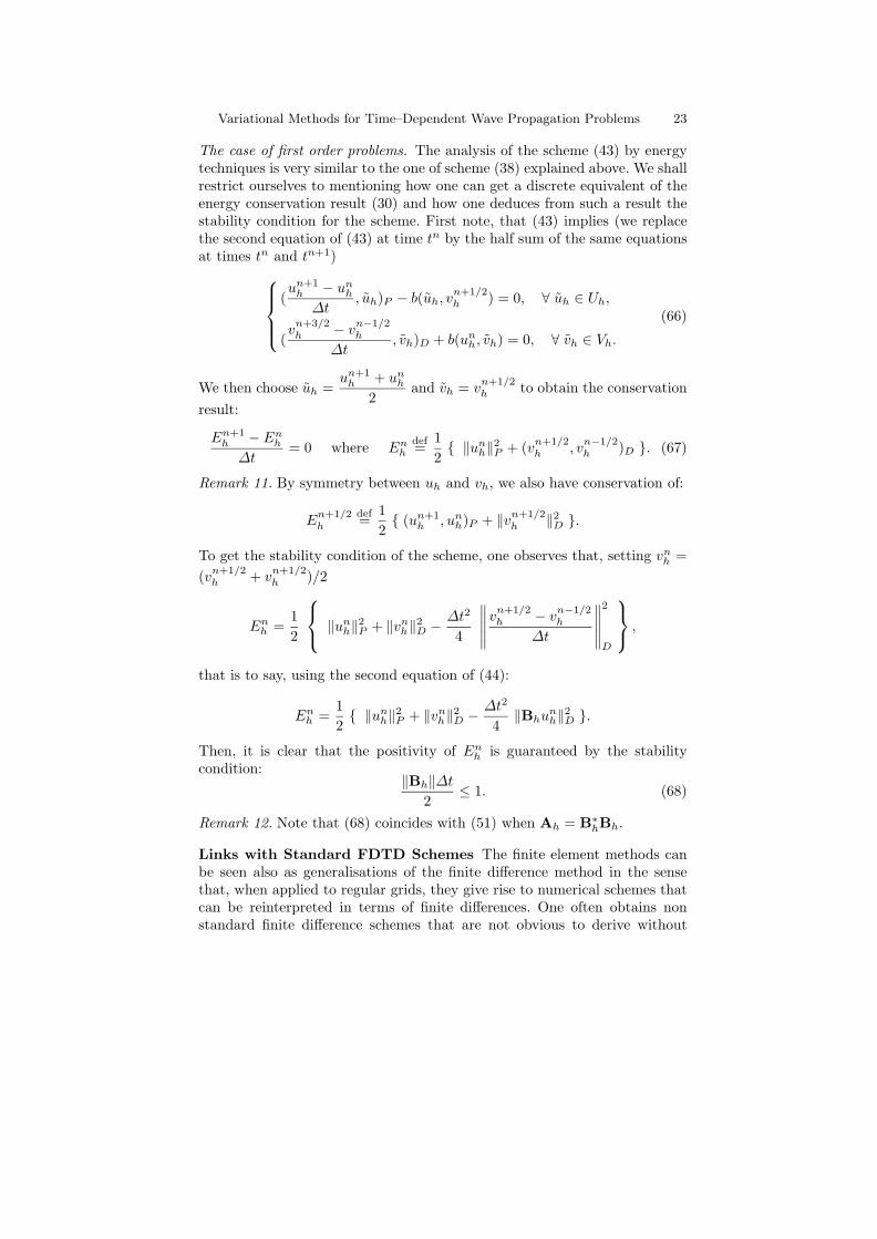
Fig. 1. The degrees of freedom for edge and face elements
thinking of the variational approach. However, one can also re-obtain classicalschemes, especially if the mass lumping procedure is applied. In such a case,the variational approach appears as an efficient way to generalise, in a stableway, finite difference schemes to variable coefficients or to treat boundaryconditions in a stable manner.
Let us give the well-known example of the Yee scheme for electromagneticsin 3D. This scheme can be recovered by applying the variational scheme (43)in the case where the scalar products (·, ·)P and (·, ·)D are given by (8) andwhere:
U = H(curl, Ω), V = L2(Ω)3 and b(e, h) =∫
Ω
curl e · h dx . (69)
One recovers the Yee scheme with a particular choice of the approximatespaces Uh and Vh and the use of a particular quadrature formula. Moreprecisely, we consider a uniform, infinite mesh Th made of equal cubes K ∈ Th
of side h. The appropriate approximation spaces are:Uh = uh ∈ U / ∀ K ∈ Th, uh|K ∈ Q0,1,1 ×Q1,0,1 ×Q1,1,0
Vh = vh ∈ H(div, Ω) / ∀ K ∈ Th, vh|K ∈ Q1,0,0 ×Q0,1,0 ×Q0,0,1 (70)
where we recall that, by definition, Qp1,p2,p3 is the set of polynomials of threevariables whose degree with respect to the ith variable is less or equal thanpi. Notice that, contrary to what one might expect, we do not use a spaceof completely discontinuous elements to approximate V = L2(Ω)3; we usevector fields whose normal component is continuous across each face of themesh. With this choice, we are in the situation described in (31):
curl Uh ⊂ Vh, (71)
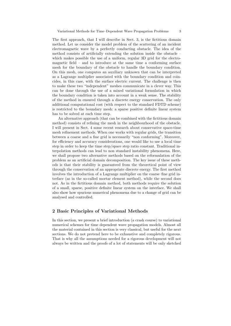
which offers a guarantee of convergence. The spaces defined by (70) are knownas edge elements for the electric field and face elements for the magnetic field(see [59]). In particular a set of degrees of freedom is given by (see also Fig. 1):
Variational Methods for Time–Dependent Wave Propagation Problems 25
– For the space Uh (degrees of freedom for the electric field): the (constant)tangential component of the vector field along each edge of the mesh.
– For the space Vh (degrees of freedom for the electric field): the (constant)tangential component of the vector field on each face of the mesh.
Remark 13. It is clear on Fig. 1, that, as far as the degrees of freedom areconcerned, the roles of the electric and magnetic fields are completely sym-metric (simply consider a “parallel” mesh shifted by h/2 in each direction).Only the interpolations of the fields are different.
Finally, in order to compute the various integrals that appear in the vari-ational formulation, we use the following numerical quadrature formula ineach cube K (which provides mass lumping):∫
K
f dx =h3
8
∑x∈SK
f(x), (72)
where SK is the set of vertices of K. Using this formula leads to the Yeescheme.
3 Fictitious Domain Methods
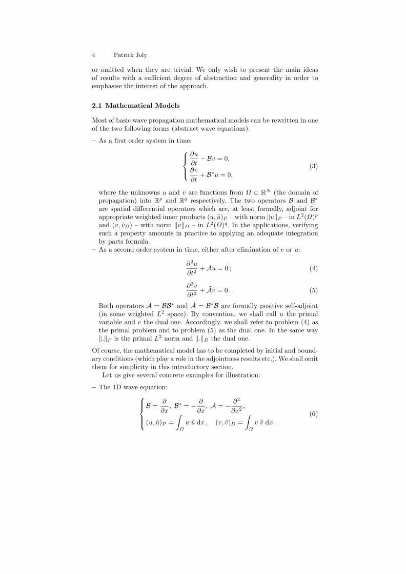
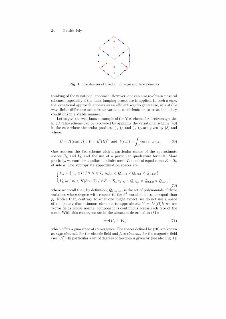
Let us consider as a model problem the propagation of waves in an exteriordomain, the complement of a bounded obstacle. The use of a standard fi-nite difference method requires a staircase approximation of the boundary ofthe obstacle (see Fig. 2) and the great disadvantage of the method is thatthis creates spurious numerical diffractions. A possibility for avoiding thisdrawback is to use a finite element method (with mass lumping). The finiteelement mesh may follow the boundary of the object exactly (see Fig. 2).
However, other drawbacks are introduced. First of all, the numerical im-plementation is much more difficult and the efficiency of the computations isdecreased by the unstructured nature of the data. Furthermore, meshing thewhole domain of computation (with tetrahedra in 3D) is expensive. Finally,the time step has to be chosen in accordance with the space mesh size (be-cause of the CFL condition), which sometimes leads to small time steps inthe presence of small elements in the mesh.
Here we investigate an alternative method for handling the scatteringproblem, namely, the fictitious domain method (denoted FDM). Such meth-ods have recently been shown to have interesting potential for solving com-plicated problems ([2–4, 39, 45, 55]) particularly in the stationary case. Theuse of the FDM for time dependent problems is relatively new [46]. How-ever, it gives very nice properties for these kinds of problems, particularlyfor exterior wave propagation. In this case, the FDM, also called the domainembedding method, consists of artificially extending the solution inside the
26 Patrick Joly
Fig. 2. Finite element mesh (left) and finite difference mesh (right)
obstacle so that the new domain of computation has a very simple shape(typically a rectangle in 2D). This extension requires the introduction of anew variable defined only at the boundary of the obstacle. This auxiliary vari-able accounts for the boundary condition, and can be related to a singularityacross the boundary of the obstacle of the extended function.
This idea will be developed in more detail in Sect. 3.1 in the case of acous-tic waves. The main point is that the mesh for the solution on the enlargeddomain can be chosen independently of the geometry of the obstacle. In par-ticular, the use of regular grids or structured meshes allows for simple andefficient computations. There is an additional cost due to the determinationof the new boundary unknown. However, the final numerical scheme is a slightperturbation of the scheme for the problem without an obstacle so this costmay be considered as marginal. Theoretically, the convergence of the methodis linked to a uniform inf-sup condition which leads to a compatibility con-dition between the boundary mesh and the uniform mesh: this implies thatthe two mesh grids cannot be chosen completely independently, but this isnot an important constraint for the applications. Another important point isthat the stability condition of the resulting scheme is the same as the one ofthe finite difference scheme.
3.1 Presentation of the Method: the Acoustic Dirichlet Problem
Our model problem is the scattering of an acoustic wave (in a homogeneousmedium with speed 1) by an obstacle O, with a Dirichlet condition on theboundary:
∂2u
∂t2− ∆u = 0, in D = Rd \ O, (d = 2 or 3)
u = 0, on γ = ∂D.(73)
We assume that the incident wave is generated by initial conditions (omittedhere) at time t = 0. In order to have a finite computational domain, theclassical technique consists of bounding the domain D and imposing absorb-ing conditions on the exterior boundary [38, 65]. For the sake of simplicity, a
Variational Methods for Time–Dependent Wave Propagation Problems 27
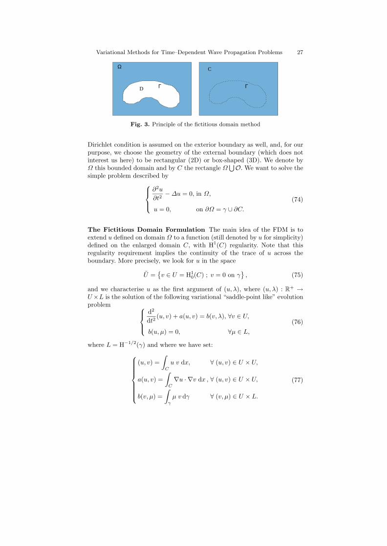
Γ
C
Γ
Ω
D
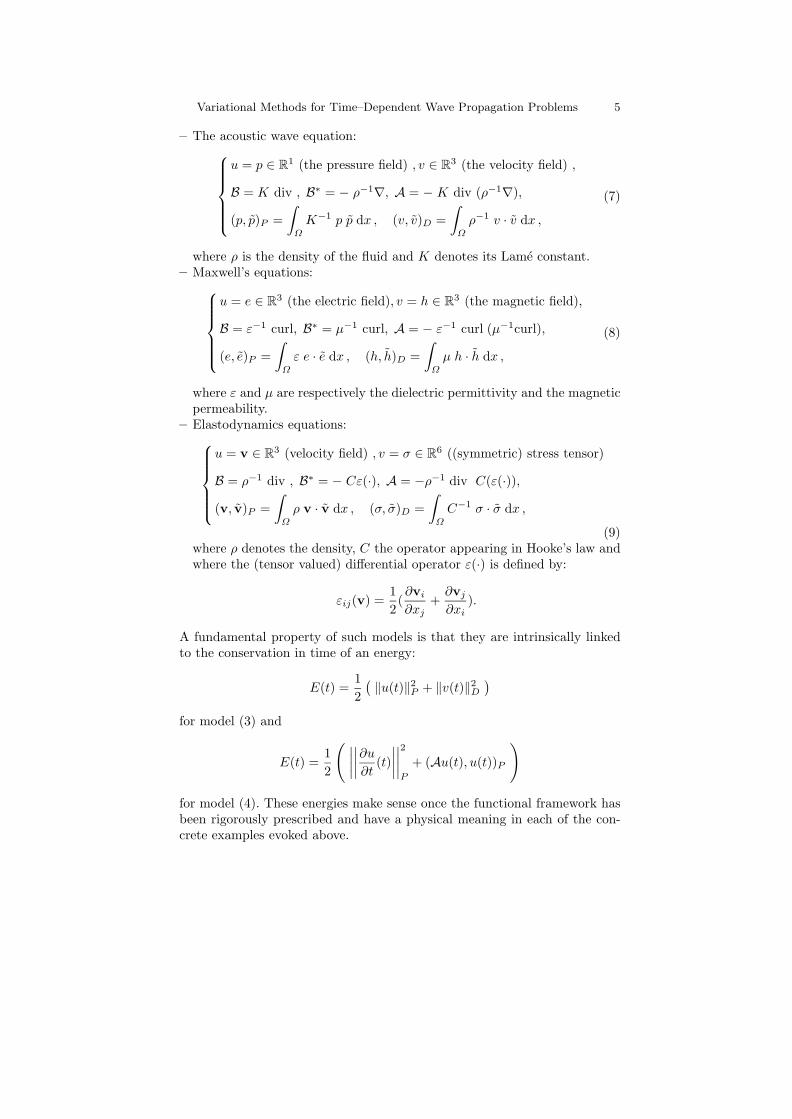
Fig. 3. Principle of the fictitious domain method
Dirichlet condition is assumed on the exterior boundary as well, and, for ourpurpose, we choose the geometry of the external boundary (which does notinterest us here) to be rectangular (2D) or box-shaped (3D). We denote byΩ this bounded domain and by C the rectangle Ω
⋃O. We want to solve the
simple problem described by∂2u
∂t2− ∆u = 0, in Ω,
u = 0, on ∂Ω = γ ∪ ∂C.
(74)
The Fictitious Domain Formulation The main idea of the FDM is toextend u defined on domain Ω to a function (still denoted by u for simplicity)defined on the enlarged domain C, with H1(C) regularity. Note that thisregularity requirement implies the continuity of the trace of u across theboundary. More precisely, we look for u in the space
U =v ∈ U = H1
0(C) ; v = 0 on γ
, (75)
and we characterise u as the first argument of (u, λ), where (u, λ) : R+ →U ×L is the solution of the following variational “saddle-point like” evolutionproblem
d2
dt2(u, v) + a(u, v) = b(v, λ), ∀v ∈ U,
b(u, µ) = 0, ∀µ ∈ L,
(76)
where L = H−1/2(γ) and where we have set:
(u, v) =∫
C
u v dx, ∀ (u, v) ∈ U × U,
a(u, v) =∫
C
∇u · ∇v dx , ∀ (u, v) ∈ U × U,
b(v, µ) =∫
γ
µ v dγ ∀ (v, µ) ∈ U × L.
(77)
28 Patrick Joly
Remark 14. Rigorously, b(u, µ) = 〈µ, u〉γ where 〈µ, u〉γ denotes the dualityproduct between L and L′. It becomes an integral over γ as soon µ ∈ L2(γ),which justifies our notation.
In essence, the method consists of first extending the solution in the en-larged computational domain and then in introducing a new unknown at theboundary. One of the main differences between this approach and a standardconforming finite element approach lies in the fact that the Dirichlet condi-tion is taken into account in a weak sense instead of being imposed in thefunctional space. In this formulation, there is no mention of the geometry ofthe problem, namely the boundary γ, in the functional space for the volumeunknown u. The geometry only appears in b(·, ·) and L. We next give twodifferent approaches to deriving (76).
How Does One Obtain the New Problem?
Via optimization theory. A first way to obtain (76) consists of freezing thetime t (as a parameter) and considering the function
f = −∂2u
∂t2(·, t),
as data. Then u = u(·, t) is the solution of the following problem−∆u = f, in Ω,
u = 0 on ∂Ω = γ ∪ ∂C(78)
and thus minimizes the functional J(v) =∫
C
12 |∇v|2 − fv
dx over the space
H10 (Ω).
This space can be seen as the space of restrictions to Ω of functions ofV defined in (75). It is then natural to consider the enlarged minimizationproblem defined by
minv∈V
J(v) =∫
C
12|∇v|2 − f v
dx, (79)
where for instance f = 0 on O and f = f on Ω. It is easy to verify thatthe restriction of the solution of problem (79) to Ω is exactly the solutionof problem (76) that we are looking for. Problem (76) can be seen as aminimization problem in U with an equality constraint on γ . Its solution isthus the first argument of the saddle point (u, λ) of the Lagrangian functionaldefined by L(v, µ) = J(v) − b(v, µ). Writing that the derivatives in v and µof this Lagrangian are equal to zero at (u, λ), we obtain:
a(u, v) = b(v, λ) + (f, v) ∀v ∈ U ,b(u, µ) = 0 ∀µ ∈ L, (80)
which gives precisely (76) with f = −utt. Here, the auxiliary unknown λ ofproblem (76) appears as the Lagrange multiplier associated with the con-straint v = 0 on γ.
Variational Methods for Time–Dependent Wave Propagation Problems 29
Via the theory of distributions. Another way to understand the system ofequations (76) is to say that, having extended u by continuity across γ andassuming that u still satisfies the wave equation inside O, (this means thatu solves the homogeneous Dirichlet problem inside and outside γ), we havein the sense of distributions in C
∂2u
∂t2− ∆u = λ δγ , (81)
where δγ is the surface measure supported on γ and λ is the jump of thenormal derivative of u across γ (this is a second “physical” reinterpretationof the auxiliary unknown) :
λ =[∂u
∂n
]. (82)
We can also interpret the multiplier λ as a source term distributed on γ. If thissource term were known, we simply would have to solve the wave equationin a square with a right hand side: the FDTD approach makes sense in sucha geometric situation. In fact, λ is unknown and becomes a control variablein order to make u satisfy the boundary condition on γ.
Multiplying (81) by a test function v ∈ U and integrating over C leads,at least formally, to the first equation of (76), the second one being the weakformulation of the fact that u vanishes on γ. This establishes an analogybetween the FDM and integral equations for scattering problems [14]. In-deed, in this kind of method λ is typically the quantity that is chosen as theunknown. Nevertheless let us point out a very important difference betweenour approach and these methods. Integral equations are known to lead, afterdiscretization, to the solution of full linear systems in λ; as will be shownlater, this is not the case for the FDM.
Finite Element Approximation and Time Discretization
Space discretization. Let Uh (respectively LH) be a finite dimensional sub-space of U (respectively L). Here h > 0 and H > 0 represent two approxi-mation parameters (a priori independent) allowed to tend to 0. In practice,they will be the stepsize of a (regular) volume mesh of C (h) and of a surfacemesh of γ (H). We approximate the variational problem (76) by
Find (uh, λH) : R+ → Uh × LH such thatd2
dt2(uh, vh) + a(uh, vh) = b(vh, λH), ∀vh ∈ Uh,
b(uh, µH) = 0, ∀µH ∈ LH .
(83)
The spaces Uh and LH will be assumed to satisfy the usual approximationproperties. Typically, Uh can be a P1 or Q1 finite element space based on aregular mesh in C, which permits us to recover a standard finite differencescheme for the wave equation. For LH , which is a subspace of H−1/2(γ), it
30 Patrick Joly
makes sense to use discontinuous functions, for instance piecewise constantfunctions on a conforming (not necessarily regular) mesh of γ. If p denotesthe dimension of Uh and q the one of LH , one gets:
p = O(h−d), q = O(H−(d−1)), (h,H → 0),
so that, since in practice H and h will be of the same order, we shall haveq ¿ p.
Using the same notation as in Sect. 2.3, it is easy to rewrite problem (83)in matrix form: Mh
d2uh
dt2+ Ahuh = B∗
HλH
BHuh = 0,
(84)
where we emphasise that :
– the mass matrix Mh is diagonal (typically the identity matrix), thanks tomass lumping,
– the stiffness matrix Ah represents a discrete Laplacian on a regular grid,– the rectangular matrix BH represents a discrete trace operator on γ.
Remark 15. The matrix BH actually depends on the both approximation pa-rameters h and H.
Problem (84) appears as a system of ordinary differential equations withan algebraic constraint. One can eliminate the time derivative of uh betweenthe two equations of (84) to obtain an equation which directly relates λH
and uh:QHλH = BHM−1
h Ahuh, QH = BHM−1h B∗
Huh. (85)
If QH , which is by construction symmetric and positive, is invertible (thisissue will be discussed in Sect. 3.1), we see that uh is the solution of theordinary differential system:
Mhd2uh
dt2+
(I − BHQ−1
H B∗H
)Ahuh = 0, (86)
which proves the existence of the discrete solution. Moreover, it is easy toprove the following energy conservation result (simply take vh as the timederivative of uh and µh = λh in (83)) :
ddt
12
(‖duh
dt(t)‖2
P + a(uh(t), uh(t)))
= 0. (87)
Variational Methods for Time–Dependent Wave Propagation Problems 31
Time discretization. According to Sect. 2.4, we shall apply the standard leapfrog procedure. With obvious notation, this leads to the following problem:
Find (unh, λn
H) ∈ Uh × LH , n > 1, such that(un+1
h − 2unh + un−1
h
∆t2, vh
)+ a(un
h, vh) = b(vh, λnH), ∀vh ∈ Uh,
b(unh, µH) = 0, ∀µH ∈ LH ,
(88)
or equivalently, in a matrix form:Mhun+1
h − 2unh + un−1
h
∆t2+ Ahun
h = B∗Hλn
H ,
BHunh = 0.
(89)
For practical computation, we shall replace the second equation of (89) byanother, which is nothing but (85) written at time tn and can be obtainedby eliminating un+1
h and un−1h between the two equations of (89):Mh
un+1h − 2un
h + un−1h
∆t2+ Ahun
h = B∗Hλn
H ,
QHλnH = BHM−1
h Ahunh.
(90)
Remark 16. One shows that (89) and (90) are equivalent if BHu0h = BHu1
h =0, which expresses in a discrete way a compatibility condition between theinitial data and the boundary condition.
Assuming that the solution is known up to time tn, the algorithm tocompute the solution at tn+1 has two steps:
– Compute un+1h via the first equation of (89) (a purely explicit step).
– Solve QHλn+1H = BHM−1
h Ahun+1h in order to compute λn+1
H (the invert-ibility of QH is thus the only condition for the existence of the discretesolution).
We see that, in comparison with a standard FDTD procedure inside C, theonly additional cost is the inversion of the matrix QH . This cost is marginal,due to the properties of QH (see Sect. 3.1). In fact, from the computationalpoint of view, the difficult step in the implementation lies in the construc-tion of the matrix BH (and then of QH): in 3D for instance, it involves thedetermination of the intersections between a cubic mesh and a surface mesh(typically with triangular plane facets). See for instance [42] for more details.
32 Patrick Joly
Theoretical Issues
Properties of the matrix QH . The following properties of the matrix QH =BHM−1
h B∗H are general, but we shall illustrate them in the case d = 2 when
we make the Q1–P0 choice:
– Q1 finite elements on a regular square mesh for the construction of Uh.– P0 (piecewise constant) finite element for the construction of LH .
We introduce the respective bases of Uh and LH :
– For Uh, wi; 1 ≤ i ≤ p where each wj is supported by 4 squares with acommon vertex.
– For LH , ϕj ; 1 ≤ j ≤ q where each ϕj is the characteristic function of a(curvilinear) segment of the mesh of γ.
Of course the entries of the matrix BH are
b(wi, ϕj) =∫
γ
wi ϕj dσ. (91)
To emphasise that QH should be easy to invert, let us observe the following.
– QH is symmetric and positive (by construction!).– QH is a “small” matrix: its dimension is exactly (q, q), to be compared
with (p, p) for AH , with p À q.– QH is a sparse matrix with narrow bandwidth. This is due to the sparsity
of the matrix BH : indeed the coefficient b(ϕi, wj) vanishes as soon as thesupports of the two basis functions (ϕj , wi) do not intersect.
The (crucial) remaining question is the definiteness of QH which correspondsto the fact that the kernel of the matrix is equal to 0, or equivalently thatBH is surjective from Uh onto LH . This suggests that the space LH mustnot be too large, or in other words that one must not impose too many“boundary”constraints to the discrete solution. As for any mixed method,there is a compatibility condition between the two spaces Uh and LH thatcan be reduced to a compatibility relation between the two meshes of C andγ: the volume mesh cannot be too large with respect to the boundary meshor, roughly speaking, the ratio H/h must be large enough. In this sense thetwo meshes cannot be completely independent.
Let us illustrate this in the Q1–P0 choice. The invertibility of QH can bereformulated as:
b(vh, µH) = 0, ∀ vh ∈ Uh =⇒ µH = 0. (92)
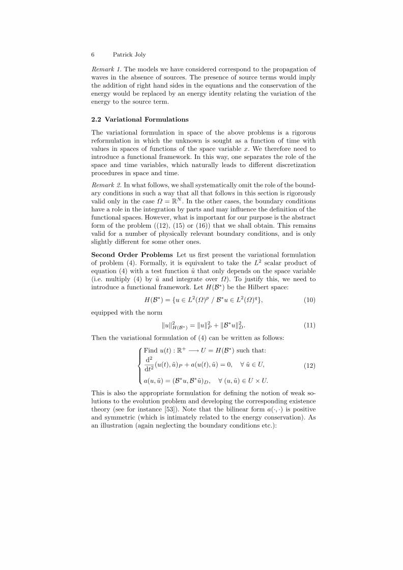
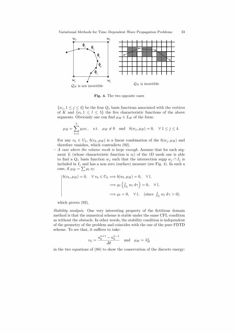
Let us consider the following opposite cases (illustrated in Fig. 4):
– A case where the volume mesh is (locally) too fine. Assume that one squareK of the 2D mesh contains 5 segments of the 1D mesh (cf. figure 4). Let
Variational Methods for Time–Dependent Wave Propagation Problems 33
w w
w
5
w
2
34
1
ϕ ϕ
ϕ
ϕ
ϕ
12
3
4
QH is not invertible
QH is invertible
Fig. 4. The two opposite cases
wj , 1 ≤ j ≤ 4 be the four Q1 basis functions associated with the verticesof K and νl, 1 ≤ l ≤ 5 the five characteristic functions of the abovesegments. Obviously one can find µH ∈ LH of the form:
µH =5∑
l=1
µlνl , s.t. µH 6= 0 and b(wj , µH) = 0, ∀ 1 ≤ j ≤ 4.
For any vh ∈ Uh, b(vh, µH) is a linear combination of the b(wj , µH) andtherefore vanishes, which contradicts (92).
– A case where the volume mesh is large enough. Assume that for each seg-ment Il (whose characteristic function is νl) of the 1D mesh one is ableto find a Q1 basis function wj such that the intersection supp wj ∩ Ij isincluded in Ij and has a non zero (surface) measure (see Fig. 4). In such acase, if µH =
∑µl νl:∣∣∣∣∣∣∣∣∣
b(vh, µH) = 0, ∀ vh ∈ Uh =⇒ b(wl, µH) = 0, ∀ l,
=⇒ µl
(∫Il
wl dγ)
= 0, ∀ l,
=⇒ µl = 0, ∀ l, (since∫
Ilwl dγ > 0).
which proves (92).
Stability analysis. One very interesting property of the fictitious domainmethod is that the numerical scheme is stable under the same CFL conditionas without the obstacle. In other words, the stability condition is independentof the geometry of the problem and coincides with the one of the pure FDTDscheme. To see that, it suffices to take:
vh =un+1
h − un−1h
∆tand µH = λn
H
in the two equations of (88) to show the conservation of the discrete energy:
34 Patrick Joly
En+1/2h =
12‖un+1
h − unh
∆t‖2
P +12
a(un+1h , un
h).
One then concludes as in Sect. 2.4.
Convergence analysis. Let us restrict ourselves to the semi-discrete problem.The convergence of the method requires a condition which is stronger than(92), namely the uniform inf-sup condition:
infµH∈LH
supvh∈Uh
b(vh, µH)‖µH‖L ‖v‖U
≥ α > 0 . (93)
Let us estimate the error between the approximate solution (uh, λh) of thesemi-discrete problem (83) and the exact solution (u, λ) of problem (76) pro-vided that this solution is regular enough. As the proof is essentially anadaptation of the one we gave in Sect. 2.3, we simply indicate its main stepsand refer to [32] for more details. Thanks to (93) and to the coercivity ofa(·, ·) in U , we can introduce the elliptic projection:∣∣∣∣∣U × L → Uh × LH
(u, λ) → (Πhu,ΠHλ)(94)
where (Πhu,ΠHλ) is defined by:a(u − Πhu, vh) = b(vh, λ − ΠHλ), ∀vh ∈ Uh,
b(u − Πhu, µH) = 0, ∀µH ∈ LH .(95)
Moreover, we have the classical result [16]:
‖u − Πhu‖U + ‖λ − ΠHλ‖L ≤ C
(inf
vh∈Uh
‖u − vh‖U + infµH∈LH
‖λ − µH‖L
).
(96)Let us write:∣∣∣∣∣uh − u = ηh − εh, ηh = uh − Πhu, εh = u − Πhu,
λH − λ = τH − θH , τH = λH − ΠHλ, θH = λ − ΠHλ.(97)
As εh and θH tend to 0 thanks to (96), it suffices to estimate ηh and τH . Oneeasily sees that:
(d2ηh
dt2, vh
)+ a(ηh, vh) − b(vh, τH) =
(d2εh
dt2, vh
), ∀vh ∈ Uh,
b(ηh, µH) = 0, ∀µH ∈ LH .
(98)
From the second equation, we deduce (we first differentiate in time this equa-tion for fixed µH and then take µH = τH):
Variational Methods for Time–Dependent Wave Propagation Problems 35
b(dηh
dt, τH) = 0.
Then taking vh =dηh
dtin the first equation of (98) leads to:
ddt
Eh = (d2εh
dt2,dηh
dt) where Eh(t) def=
12 ‖dηh
dt(t)‖2
P + a(ηh(t), ηh(t)) .(99)
One then concludes as in Sect. 2.3 to get the estimate of Eh and thus of ηh.Finally, to get an estimate for τH , we use the uniform inf-sup condition:
‖τH‖L ≤ α−1 supvh∈Uh
b(vh, τH)‖vh‖U
. (100)
From the first equation of (98) we deduce that:
|b(vh, τH)| ≤ C
‖d2ηh
dt2‖ + ‖ηh‖U + ‖εh‖
‖vh‖U ,
so that finally:
‖τH‖L ≤ C
‖d2ηh
dt2‖ + ‖ηh‖U + ‖εh‖
, (101)
which means essentially that one controls τH in terms of quantities whichhave already been estimated (ηh and ηh). We refer the reader to [32] for thedetails.
Accuracy of the fictitious domain method. The counterpart to the good prop-erties of the fictitious domain method, in terms of simplicity and robustness,is its limited accuracy. As a matter of fact, the convergence proof shows thatthe accuracy is essentially driven by the “interpolation error” associated withthe exact solution (u, λ) of the continuous problem :
infvh∈Uh
‖u − vh‖U + infµH∈LH
‖λ − µH‖L
(and the same quantity where (u, λ) are replaced by successive time deriva-tives). The limitation of the accuracy is then due to the fact that the regu-larity of the exact solution in C – or inside an element K of the volume mesh– is limited, independently of the smoothness of the data of the problem,by the fact that the normal derivative of u presents a jump across γ. As aconsequence, the maximal space regularity for u(·, t) is (it is the same fortime derivatives):
u(·, t) ∈ H3/2−ε(C), ∀ ε > 0.
As a consequence we simply have:
36 Patrick Joly
infvh∈Uh
‖u(·, t) − vh‖U ≤ C(ε, u) h1/2−ε
while, as soon as λ(·, t) ∈ H1/2(γ):
infµH∈LH
‖λ(·, t) − µH‖L ≤ C(λ) H.
Then the convergence analysis provides the following error estimates in which,for clarity, we make explicit the Sobolev norms that are used (see [44] for amore rigorous presentation):
‖u(·, t)−uh(·, t)‖H1(C)+‖λ(·, t)−λH(·, t)‖H−1/2(γ) ≤ C(ε, u, λ)(h1/2−ε + H
).
(102)Using classical duality arguments it is possible to get an estimate of u(·, t)−uh(·, t) in L2 (see again [44] in the elliptic case):
‖u(·, t)−uh(·, t)‖L2(C) +‖λ(·, t)−λH(·, t)‖H−1/2(γ) ≤ C(ε, u, λ)(h1−ε + H
).
(103)This last estimate shows that the fictitious domain method is essentially oforder 1.
About the uniform inf-sup condition. It is natural to look at what kind ofcompatibility relation between the two meshes implies the uniform inf-supcondition. We already saw that, in the Q1–P0 case, the invertibility of QH
would require a sufficiently fine mesh. It appears that the same kind of con-dition, namely:
H ≥ C h, (104)
is sufficient for the uniform inf-sup condition. One can describe a very gen-eral procedure to prove such a result (inspired in particular by the work ofBabuska [5]). One wants to show that:
∀µH ∈ LH ,∃ vh ∈ Uh / bΓ (µH , vh) ≥ α ‖µH‖L ‖vh‖U (105)
for some α > 0, at least for a ratio h/H small enough.For this, it is sufficient to have the two following properties:
1. One can construct R ∈ L(L,U) such that
∀µ ∈ L, bΓ (µ,Rµ) ≥ ‖Rµ‖2U , ‖Rµ‖U ≥ ν ‖µ‖L (106)
which obviously provides a proof for the continuous inf-sup condition.2. One can construct an “interpolation “ operator Πh ∈ L(U,Uh) such that
∀µH ∈ LH , ‖RµH − ΠhRµH‖U ≤ o(h
H) ‖µH‖2
L. (107)
Variational Methods for Time–Dependent Wave Propagation Problems 37
Indeed, let us assume that these two criteria are fulfilled. For µH ∈ LH , toobtain (105), we choose vh = ΠhRµH , then:∣∣∣∣∣∣∣∣∣
bΓ (µH , vh) = bΓ (µH ,ΠhRµH),
= bΓ (µH ,RµH) + bΓ (µH , µH − ΠhRµH),
≥ ‖RµH‖2U − o(
h
H) ‖µH‖2
L.
We then use the inequalities:∣∣∣∣∣ ‖RµH‖2U ≥ ν ‖µH‖L ‖RµH‖U ,
‖µH‖2L ≤ ν−1 ‖µH‖L ‖RµH‖U ,
to conclude that:
bΓ (µH , vh) ≥ ν − ν−1 o(h/H) ‖µH‖L ‖vh‖U ,
which proves the inf-sup condition for h/H small enough.Let us apply this to our model problem (U = H1
0 (C), L = H−1/2(Γ ) andQ1–P0 finite elements for Uh × LH). For criterion 1, we construct u = Rµ ∈H1(C) as:
−∆u + u = 0, in C
[u]Γ = 0, [∂u
∂n]Γ = µ on Γ .
By Green’s formula:
bΓ (µ, u) =∫
Γ
µ u dγ =∫
C
( |∇u|2 + |u|2) dx = ‖Rµ‖21,C ,
and by the trace theorem:
‖µ‖−1/2,Γ ≤ C ( ‖u‖1,C + ‖∆u‖0,C) ≤ C ‖u‖1,C = C ‖Rµ‖1,C ,
which satisfies criterion 1. Moreover, we have the estimate :
‖u‖1,Ω = ‖Rµ‖1,Ω ≤ C ‖µ‖−1/2,Γ
and also, by a regularity result:
µ ∈ Hs−1/2(Γ ) ⇔ ‖Rµ‖1+s,Ω ≤ C(s) ‖µ‖s−1/2,Γ ,
where s = 1/2− ε (where ε > 0 can be arbitrarily small). To show that crite-rion 2 is satisfied for the Q1–P0 choice, let Πh be the orthogonal projectionin H1
0 (C) from U to Uh:
∀u ∈ H2(Ω), ‖u − Πhu‖1,Ω ≤ C h ‖u‖2,Ω .
38 Patrick Joly
By interpolation, for 1 ≤ q ≤ 2:
∀u ∈ H1+q(Ω), ‖u − Πhu‖1,Ω ≤ Cq hq ‖u‖1+q,Ω .
Since LH ⊂ Hq−1/2(Γ ) for any 0 ≤ q < 1, we have, with s = 1/2 − ε:
‖RµH − ΠhRµH‖1,Ω ≤ Cs hs ‖RµH‖1+s,Ω . ≤ Cs C(s) hs ‖µ‖s−1/2,Γ
Now, we assume, that the meshes of γ form a uniformly regular family ofmeshes (see [5]). In such a case, we have an inverse inequality:
‖µ‖s−1/2,Γ ≤ H−s ‖µ‖−1/2,Γ
so that finally:
‖RµH − ΠhRµH‖1,Ω ≤ Cs C(s)(
h
H
)s
‖µ‖s−1/2,Γ ,
which is nothing but (107).
Remark 17. The main drawback of this “very general” type of proof is thatit does not provide an explicit numerical value for the constant C in theinequality (104). In [44], Girault and Glowinski have obtained an explicitvalue for C in the case of the elliptic problem corresponding to our 2D modelproblem. Their proof is technically difficult and relies on the construction of aso-called Fortin’s operator. This construction uses the Clement’s interpolationoperator [23], that is known to exist for Lagrange finite elements. That is whythis proof is not directly generalisable to other equations (such as Maxwell’sequations).
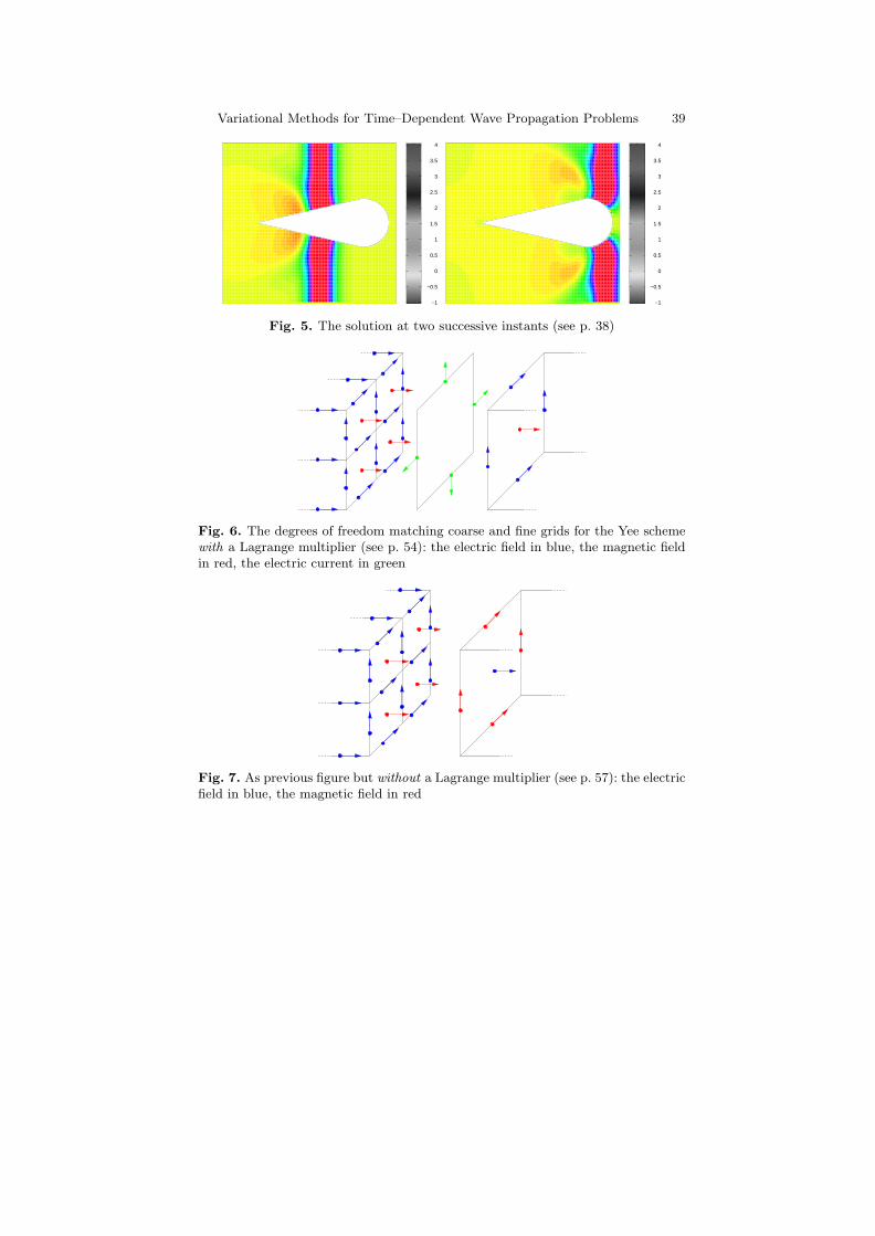
A Numerical Experiment. Here we show a numerical experiment todemonstrate that the fictitious domain method provides better accuracy thana staircase approximation of the boundary. We want to compute the diffrac-tion of an incident plane wave by a “2D cone-sphere”. In this case, γ is theunion of one half-circle with two segments. The geometry of the problem isclear in Fig. 5 on p. 39. The incident wave is a plane wave, with Gaussianpulse, coming from the left of the picture and propagating to the right.
We represent two snapshots of the solution of the problem in Fig. 5. Weclearly distinguish on these pictures the incident wave and the scattered field.
Next we want to compare the convergence of the fictitious domain methodwith the one of the pure FDTD approach combined with a staircase approx-imation of the boundary γ. To do that, we look at the solution at point ashort distance to the left of the sharp tip as a function of time for 1 ≤ t ≤ 3,which corresponds to the passage of the scattered field. In each case we havecomputed the discrete solutions for three values of the stepsize h which cor-respond approximately to 10, 20 and 40 points per wavelength of the incidentwave. The ratio h/H is kept constant.
Variational Methods for Time–Dependent Wave Propagation Problems 39
−1
−0.5
0
0.5
1
1.5
2
2.5
3
3.5
4
−1
−0.5
0
0.5
1
1.5
2
2.5
3
3.5
4
Fig. 5. The solution at two successive instants (see p. 38)
Fig. 6. The degrees of freedom matching coarse and fine grids for the Yee schemewith a Lagrange multiplier (see p. 54): the electric field in blue, the magnetic fieldin red, the electric current in green
Fig. 7. As previous figure but without a Lagrange multiplier (see p. 57): the electricfield in blue, the magnetic field in red
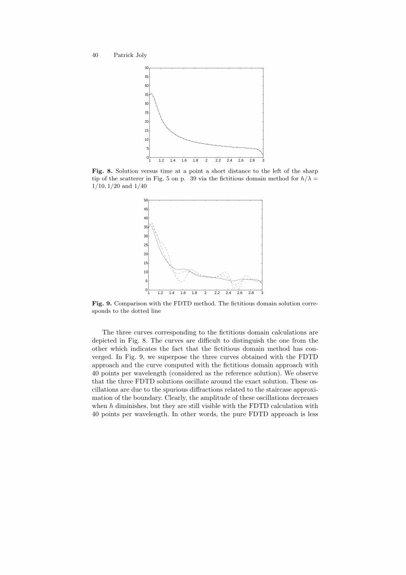
40 Patrick Joly
1 1.2 1.4 1.6 1.8 2 2.2 2.4 2.6 2.8 30
5
10
15
20
25
30
35
40
45
50
Fig. 8. Solution versus time at a point a short distance to the left of the sharptip of the scatterer in Fig. 5 on p. 39 via the fictitious domain method for h/λ =1/10, 1/20 and 1/40
1 1.2 1.4 1.6 1.8 2 2.2 2.4 2.6 2.8 30
5
10
15
20
25
30
35
40
45
50
Fig. 9. Comparison with the FDTD method. The fictitious domain solution corre-sponds to the dotted line
The three curves corresponding to the fictitious domain calculations aredepicted in Fig. 8. The curves are difficult to distinguish the one from theother which indicates the fact that the fictitious domain method has con-verged. In Fig. 9, we superpose the three curves obtained with the FDTDapproach and the curve computed with the fictitious domain approach with40 points per wavelength (considered as the reference solution). We observethat the three FDTD solutions oscillate around the exact solution. These os-cillations are due to the spurious diffractions related to the staircase approxi-mation of the boundary. Clearly, the amplitude of these oscillations decreaseswhen h diminishes, but they are still visible with the FDTD calculation with40 points per wavelength. In other words, the pure FDTD approach is less
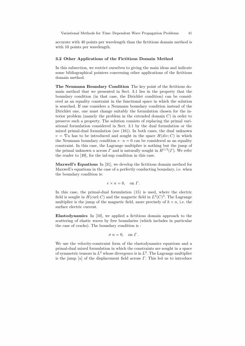
Variational Methods for Time–Dependent Wave Propagation Problems 41
accurate with 40 points per wavelength than the fictitious domain method iswith 10 points per wavelength.
3.2 Other Applications of the Fictitious Domain Method
In this subsection, we restrict ourselves to giving the main ideas and indicatesome bibliographical pointers concerning other applications of the fictitiousdomain method.
The Neumann Boundary Condition The key point of the fictitious do-main method that we presented in Sect. 3.1 lies in the property that theboundary condition (in that case, the Dirichlet condition) can be consid-ered as an equality constraint in the functional space in which the solutionis searched. If one considers a Neumann boundary condition instead of theDirichlet one, one must change suitably the formulation chosen for the in-terior problem (namely the problem in the extended domain C) in order topreserve such a property. The solution consists of replacing the primal vari-ational formulation considered in Sect. 3.1 by the dual formulation or themixed primal-dual formulation (see (16)). In both cases, the dual unknownv = ∇u has to be introduced and sought in the space H(div;C) in whichthe Neumann boundary condition v · n = 0 can be considered as an equalityconstraint. In this case, the Lagrange multiplier is nothing but the jump ofthe primal unknown u across Γ and is naturally sought in H1/2(Γ ). We referthe reader to [49], for the inf-sup condition in this case.
Maxwell’s Equations In [31], we develop the fictitious domain method forMaxwell’s equations in the case of a perfectly conducting boundary, i.e. whenthe boundary condition is:
e × n = 0, on Γ .
In this case, the primal-dual formulation (15) is used, where the electricfield is sought in H(curl;C) and the magnetic field in L2(C)3. The Lagrangemultiplier is the jump of the magnetic field, more precisely of h × n, i.e. thesurface electric current.
Elastodynamics In [10], we applied a fictitious domain approach to thescattering of elastic waves by free boundaries (which includes in particularthe case of cracks). The boundary condition is :
σ n = 0, on Γ .
We use the velocity-constraint form of the elastodynamics equations and aprimal-dual mixed formulation in which the constraints are sought in a spaceof symmetric tensors in L2 whose divergence is in L2. The Lagrange multiplieris the jump [u] of the displacement field across Γ . This led us to introduce
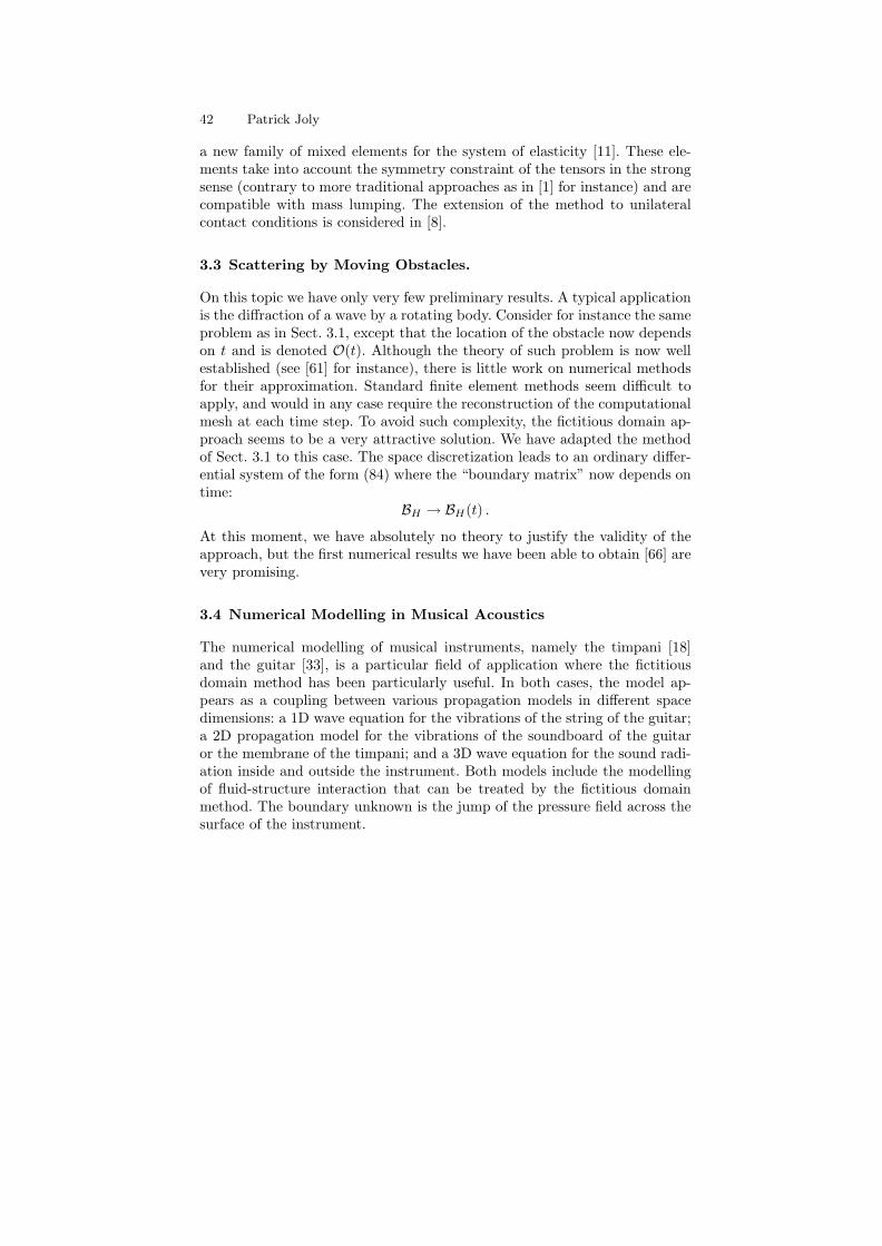
42 Patrick Joly
a new family of mixed elements for the system of elasticity [11]. These ele-ments take into account the symmetry constraint of the tensors in the strongsense (contrary to more traditional approaches as in [1] for instance) and arecompatible with mass lumping. The extension of the method to unilateralcontact conditions is considered in [8].
3.3 Scattering by Moving Obstacles.
On this topic we have only very few preliminary results. A typical applicationis the diffraction of a wave by a rotating body. Consider for instance the sameproblem as in Sect. 3.1, except that the location of the obstacle now dependson t and is denoted O(t). Although the theory of such problem is now wellestablished (see [61] for instance), there is little work on numerical methodsfor their approximation. Standard finite element methods seem difficult toapply, and would in any case require the reconstruction of the computationalmesh at each time step. To avoid such complexity, the fictitious domain ap-proach seems to be a very attractive solution. We have adapted the methodof Sect. 3.1 to this case. The space discretization leads to an ordinary differ-ential system of the form (84) where the “boundary matrix” now depends ontime:
BH → BH(t) .
At this moment, we have absolutely no theory to justify the validity of theapproach, but the first numerical results we have been able to obtain [66] arevery promising.
3.4 Numerical Modelling in Musical Acoustics
The numerical modelling of musical instruments, namely the timpani [18]and the guitar [33], is a particular field of application where the fictitiousdomain method has been particularly useful. In both cases, the model ap-pears as a coupling between various propagation models in different spacedimensions: a 1D wave equation for the vibrations of the string of the guitar;a 2D propagation model for the vibrations of the soundboard of the guitaror the membrane of the timpani; and a 3D wave equation for the sound radi-ation inside and outside the instrument. Both models include the modellingof fluid-structure interaction that can be treated by the fictitious domainmethod. The boundary unknown is the jump of the pressure field across thesurface of the instrument.
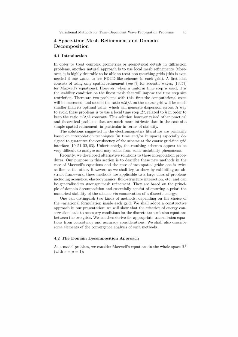
Variational Methods for Time–Dependent Wave Propagation Problems 43
4 Space-time Mesh Refinement and DomainDecomposition
4.1 Introduction
In order to treat complex geometries or geometrical details in diffractionproblems, another natural approach is to use local mesh refinements. More-over, it is highly desirable to be able to treat non matching grids (this is evenneeded if one wants to use FDTD-like schemes in each grid). A first ideaconsists of using only spatial refinement (see [7] for acoustic waves, [13, 57]for Maxwell’s equations). However, when a uniform time step is used, it isthe stability condition on the finest mesh that will impose the time step sizerestriction. There are two problems with this: first the computational costswill be increased; and second the ratio c∆t/h on the coarse grid will be muchsmaller than its optimal value, which will generate dispersion errors. A wayto avoid these problems is to use a local time step ∆t, related to h in order tokeep the ratio c∆t/h constant. This solution however raised other practicaland theoretical problems that are much more intricate than in the case of asimple spatial refinement, in particular in terms of stability.
The solutions suggested in the electromagnetics literature are primarilybased on interpolation techniques (in time and/or in space) especially de-signed to guarantee the consistency of the scheme at the coarse grid-fine gridinterface [19, 51, 52, 63]. Unfortunately, the resulting schemes appear to bevery difficult to analyse and may suffer from some instability phenomena.
Recently, we developed alternative solutions to these interpolation proce-dures. Our purpose in this section is to describe these new methods in thecase of Maxwell’s equations and the case of two spatial grids: one is twiceas fine as the other. However, as we shall try to show by exhibiting an ab-stract framework, these methods are applicable to a large class of problemsincluding acoustics, elastodynamics, fluid-structure interaction, etc. and canbe generalised to stronger mesh refinement. They are based on the princi-ple of domain decomposition and essentially consist of ensuring a priori thenumerical stability of the scheme via conservation of a discrete energy.
One can distinguish two kinds of methods, depending on the choice ofthe variational formulation inside each grid. We shall adopt a constructiveapproach in our presentation: we will show that the criterion of energy con-servation leads to necessary conditions for the discrete transmission equationsbetween the two grids. We can then derive the appropriate transmission equa-tions from consistency and accuracy considerations. We shall also describesome elements of the convergence analysis of such methods.
4.2 The Domain Decomposition Approach
As a model problem, we consider Maxwell’s equations in the whole space R3
(with ε = µ = 1):
44 Patrick Joly
f
n
n
c
Fig. 10. 2D slice of the do-mains Ωf and Ωc.
Fig. 11. 3D view of the re-finement
∂e
∂t− curl h = 0, x ∈ R3
∂h
∂t+ curl e = 0, x ∈ R3
(108)
Our goal is to solve this problem numerically by domain decomposition usinglocally a grid twice as fine as in the rest of the domain. To be more precise, weconsider a box Ωf with boundary Σ (with outward and unit normal vectorn), and Ωc denoting the exterior of Ωf . The domain Ωf is the one that weshall discretize with a fine grid of stepsize h and Ωc is the one that we shalldiscretize with a coarse grid of step 2h (see Fig. 4.2). In what follows, (ec, hc)(resp. (ef , hf )) will denote the restriction to Ωc (resp. Ωf ) of (e, h). Sayingthat (e, h) is solution of (108) is equivalent to saying that (ec, hc) and (ef
hf ) are solutions of the same equations (108) respectively in Ωc and Ωf andare coupled by the following transmission conditions (the continuity of thetangential traces of the two fields across Σ):
n × (ec × n) = n × (ef × n) on Σ ,
hc × n = hf × n on Σ .(109)
4.3 Variational Formulations
A Variational Formulation with Lagrange Multiplier This formula-tion is similar to the fictitious domain formulation we presented in Sect. 3.1.We introduce as an additional unknown, a Lagrange multiplier, namely thecommon tangential trace of the magnetic fields hc and hf on the interface:
j(x, t) = (hf ∧ n)|Σ = (hc ∧ n)|Σ . (110)
Note that j is nothing other than the surface electric current on Σ. Wecan then reformulate our problem as follows. Assuming for a moment that
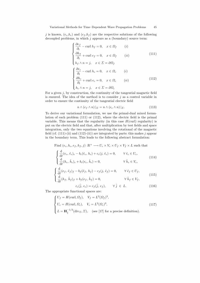
Variational Methods for Time–Dependent Wave Propagation Problems 45
j is known, (ec,hc) and (ef ,hf ) are the respective solutions of the followingdecoupled problems, in which j appears as a (boundary) source term:
∂ef
∂t− curl hf = 0, x ∈ Ωf (i)
∂hf
∂t+ curl ef = 0, x ∈ Ωf (ii)
hf ∧ n = j, x ∈ Σ = ∂Ωf
(111)
∂ec
∂t− curl hc = 0, x ∈ Ωc (i)
∂hc
∂t+ curl ec = 0, x ∈ Ωc (ii)
hc ∧ n = j, x ∈ Σ = ∂Ωc
(112)
For a given j, by construction, the continuity of the tangential magnetic fieldis ensured. The idea of the method is to consider j as a control variable inorder to ensure the continuity of the tangential electric field
n ∧ (ef ∧ n) |Σ = n ∧ (ec ∧ n) |Σ . (113)
To derive our variational formulation, we use the primal-dual mixed formu-lation of each problem (111) or (112), where the electric field is the primalvariable. This means that the regularity (in this case H(curl) regularity) isput on the electric field and that, after multiplication by test fields and spaceintegration, only the two equations involving the rotational of the magneticfield (cf. (111)-(ii) and (112)-(ii)) are integrated by parts: this makes j appearin the boundary term. This leads to the following abstract formulation:
Find (ec, hc, ef , hf , j) :R+ −→ Uc × Vc × Uf × Vf × L such thatddt
(ec, ec)c − bc(ec, hc) + cc(j, ec) = 0, ∀ ec ∈ Uc,
ddt
(hc, hc)c + bc(ec, hc) = 0, ∀ hc ∈ Vc,
(114)
ddt
(ef , ef )f − bf (ef , hf ) − cf (j, ef ) = 0, ∀ ef ∈ Uf ,
ddt
(hf , hf )f + bf (ef , hf ) = 0, ∀ hf ∈ Vf ,
(115)
cc(j, ec) = cf (j, ef ), ∀ j ∈ L. (116)
The appropriate functional spaces are:Uf = H(curl, Ωf ), Vf = L2(Ωf )3,
Uc = H(curl, Ωc), Vc = L2(Ωc)3,
L = H−1/2‖ (divΣ , Σ), (see [17] for a precise definition).
(117)
46 Patrick Joly
The space L is nothing but the image of the spaces Vf and Vc by the tracemap
γτu = u ∧ n|Σ .
The various bilinear forms appearing in (114), (115) and (116) are definedby:
(uc, uc)c =∫
Ωcuc · uc dx, (uf , uf )f =
∫Ωf
uf · uf dx,
bc(ec, hc) =∫
Ωchc · curl ec dx, bf (ef , hf ) =
∫Ωf
hf · curl ef dx,
cc(j, ec) = < j, πτec >, cf (j, ef ) = < j, πτef > .
(118)
where πτ denotes the trace map:
πτu = n ∧ (u ∧ n)|Σ ,
that maps the spaces Vf and Vc continuously onto the dual space of L, L′ =H−1/2
⊥ (curlΣ , Σ). Finally, we shall denote by < ·, · > the duality productbetween L and L′, natural extension of the usual scalar product in L2(Σ)3.
A Variational Formulation Without Lagrange Multiplier One canavoid the introduction of a Lagrange multiplier by coupling a primal-dualformulation in Ωf (the regularity is on the electric field) with a dual-primalformulation in Ωc (the regularity is on the magnetic field). In the domain Ωf ,we multiply equations (111) (i) and (ii) by test fields and apply an integrationby parts to the first equality. This leads to:
ddt
∫Ωf
ef · ef (x) dx −∫
Ωf
curl ef ·hf dx − < γτhf , πτ ef > = 0.
To get rid of γτhf , which does not make sense if we look for hf in L2, weuse the transmission condition, to replace γτhf by γτhc, which makes sensesince we shall look for hc in H(curl):
ddt
∫Ωf
ef · ef (x) dx −∫
Ωf
curl ef ·hf dx − < γτhc, πτ ef > = 0.
In the domain Ωf , we proceed in the same manner except that the roles ofthe electric and magnetic fields are exchanged. Finally, we end up with thefollowing variational formulation:
Find (ec, hc, ef , hf ) :R+ −→ Uc × Vc × Uf × Vf such thatddt
(ec, ec)c − bc(ec, hc) = 0, ∀ ec ∈ Uc,
ddt
(hc, hc)c + bc(ec, hc) + c(ef , hc) = 0, ∀ hc ∈ Vc,
(119)
Variational Methods for Time–Dependent Wave Propagation Problems 47ddt
(ef , ef )f − bf (ef , hf ) − c(ef , hc) = 0, ∀ ef ∈ Uf ,
ddt
(hf , hf )f + bf (ef , hf ) = 0, ∀ hf ∈ Vf ,
(120)
where we have set:Uf = H(curl, Ωf ), Vf = L2(Ωf )3,
Uc = L2(Ωc)3, Vc = H(curl, Ωc),(121)
bc(ec, hc) =∫
Ωchc · curl ec dx, bf (ef , hf ) =
∫Ωf
curl hf · ef dx,
c(ec, hf ) = < γτhc, πτef > = < γτef , πτhc > .
(122)
4.4 Finite Element Approximation
The Case with Lagrange Multiplier We consider here the space dis-cretization of ((114), (115), (116)). We introduce
Uc,h ⊂ Uc, Vc,h ⊂ Vc, Uf,h ⊂ Uf , Vf,h ⊂ Vf and Lh ⊂ L, (123)
some finite dimensional approximation subspaces. In practise these spaces willbe constructed as finite element spaces associated with two different meshesof Ωf and Ωc, the typical situation being that the space step in the coarsegrid domain Ωc is twice as large as that in the fine grid domain Ωf .
Find (ec,h, hc,h, ef,h, hf,h, jh) :R+ −→ Uc,h × Vc,h × Uf,h × Vf,h × L such thatddt
(ec,h, ec,h)c − bc(ec,h, hc,h) + cc(jh, ec,h) = 0, ∀ ec,h ∈ Uc,h,
ddt
(hc,h, hc,h)c + bc(ec,h, hc,h) = 0, ∀ hc,h ∈ Vc,h,
(124)ddt
(ef,h, ef,h)f − bf (ef,h, hf,h) − cf (jh, ef,h) = 0, ∀ ef,h ∈ Uf,h,
ddt
(hf,h, hf,h)f + bf (ef,h, hf,h) = 0, ∀ hf,h ∈ Vf,h,
(125)cc(jh, ec,h) = cf (jh, ef,h), ∀ jh ∈ Lh, (126)
which can be rewritten as an algebraic-differential system (we omit the sub-script h):
48 Patrick Joly
MEf
def
dt− Bf hf − C∗
f j = 0,
MHf
dhf
dt+ B∗
f ef = 0,
MEc
dec
dt− Bc hc + C∗
c j = 0,
MHc
dhc
dt+ B∗
c ec = 0,
Cc ec − Cf ef = 0.
(127)
As for the fictitious domain method, this system can be (theoretically) re-duced to a standard ordinary differential system, through the elimination ofj. Indeed, it is easy to derive from (127) the following stationary relationbetween j and (hf ,hc):(Cc
(ME
c
)−1 C∗c + Cf
(ME
f
)−1 C∗f
)j = Cc
(ME
c
)−1 Bchc − Cf
(ME
f
)−1 Bfhf .
(128)This shows that the well-posedness of (127) is conditioned by the invertibilityof the matrix:
Q = Cc
(ME
c
)−1 C∗c + Cf
(ME
f
)−1 C∗f , (129)
which is also equivalent to:
Ker C∗f ∩ Ker C∗
c = 0 . (130)
Remark 18. The conditions (130), that can also be expressed in terms of aninf-sup condition, represent once again a compatibility between the spacesUc,h, Uf,h and Lh. In particular, it is clear again that the space Lh must notbe too large. That is why, in practice, we shall often use as the boundarymesh for Σ the trace of the coarse grid mesh for Ωc.
The Case Without Lagrange Multiplier This situation is simpler. Wekeep here the notation (123) for the approximation spaces (except that Lh
does not exist any longer). The semi-discrete problem to be solved is:
Find (ec,h, hc,h, ef,h, hf,h) :R+ −→ Uc,h × Vc,h × Uf,h × Vf,h such thatddt
(ec,h, ec,h)c − bc(ec,h, hc,h) = 0, ∀ ec,h ∈ Uc,h,
ddt
(hc,h, hc,h)c + bc(ec,h, hc,h) + c(ef,h, hc,h) = 0, ∀ hc,h ∈ Vc,h,
(131)ddt
(ef,h, ef,h)f − bf (ef,h, hf,h) − c(ef,h, hc,h) = 0, ∀ ef,h ∈ Uf,h,
ddt
(hf,h, hf,h)f + bf (ef,h, hf,h) = 0, ∀ hf ∈ Vf,h,
(132)
Variational Methods for Time–Dependent Wave Propagation Problems 49
which leads directly to an ordinary differential system:
MEf
def
dt− Bf hf = 0,
MHf
dhf
dt+ B∗
f ef − C∗ hc = 0,
MEc
dec
dt− Bc hc + C ef = 0,
MHc
dhc
dt+ B∗
c ec = 0.
(133)
Remark 19. Note that in this case there is no particular requirement for thesemi-discrete problem to be well-posed.
4.5 Time Discretization
The Case with Lagrange Multiplier
The interior schemes. We look for a time discretization scheme for ((124),(125), (126)) that will use a time step ∆t in Ωf and a time step 2∆t in Ωg.More precisely:
– In Ωf , the discrete interior unknowns will be enf,h, h
n+1/2f,h .
– In Ωc, the discrete interior unknowns will be e2nc,h, h2n+1
c,h .
With such a choice, the two computational grids only meet at “even instants”t = t2n at which the two electric fields (in Ωc and Ωf ) will be computedsimultaneously. Concerning the interface unknown jh, the definition (110)(this is also clear in system (127)) suggests that the electric current must becomputed at the same instants than the magnetic field. This leads a priorito consider two different ways to discretize jh:
– If j is considered as the tangential trace of hc, in which case we denote itjc, one would like to compute it at times t2n+1: j2n+1
c,h .– If j is considered as the tangential trace of hc, in which case we denote it
jf , one would like to compute it at times t2n+1: jn+1/2f,h .
Then we use a standard staggered second order approximation in time for(114) and (115). For the time interval [t2n, t2n+2], this amounts to consideringthe following set of equations:
(e2n+1f,h − e2n
f,h
∆t, ef,h
)f
− bf (ef,h, h2n+1/2f,h ) − cf (j2n+1/2
f,h , ef,h) = 0,
(h
2n+1/2f,h − h
2n−1/2f,h
∆t, hf,h
)f
+ bf (e2nf,h, hf,h) = 0,
(134)
50 Patrick Joly
(e2n+2f,h − e2n+1
f,h
∆t, ef,h
)f
− bf (ef,h, h2n+3/2f,h ) − cf (j2n+3/2
f,h , ef,h) = 0,
(h
2n+3/2f,h − h
2n+1/2f,h
∆t, hf,h
)f
+ bf (e2n+1f,h , hf,h) = 0,
(135)∀ ef,h ∈ Uf,h, ∀hf,h ∈ Vf,h,
(e2n+2c,h − e2n
c,h
∆t, ec,h
)c
− bc(ec,h, h2n+1c,h ) + cc(j2n+1
c,h , ec,h) = 0,(h2n+1
c,h − h2n−1c,h
∆t, hc,h
)c
+ bc(e2nc,h, hc,h) = 0,
(136)
∀ ec,h ∈ Uc,h, ∀ hc,h ∈ Vc,h.
To complete our scheme we must explain how we couple the two gridsthrough discrete transmission conditions that will induce:
– the continuity of the tangential trace of the magnetic field, namely theequality:
jc = jf , (137)
– the continuity (in the weak sense) of the tangential trace of the electricfield, namely the equation:
cc(jh, ec,h) = cf (jh, ef,h), ∀ jh ∈ Lh. (138)
This should be achieved with a guarantee of stability for the coupled system.It is the most delicate point and, for the construction, we will be guided byan energy analysis.
Energy conservation and transmission scheme. According to what we haveseen in Sect. 2.4, one can define fine and coarse grid energies as follows:
Enf,h =
12
(‖en
f,h‖2f + (hn+1/2
f,h , hn+1/2f,h )f
),
E2nc,h =
12
(‖e2n
c,h‖2c + (hn+1/2
c,h , hn+1/2c,h )c
).
(139)
The total energy can only be defined at even instants:
E2nh = E2n
f,h + E2nc,h. (140)
We are looking for a conservative scheme, i.e. a scheme that will enforce theequality:
E2n+2h = E2n
h . (141)
Variational Methods for Time–Dependent Wave Propagation Problems 51
Then, by construction, the L2 stability of the coupled scheme will be ensuredunder the double strict CFL stability condition (the proof is the same as inSect. 2.4 ):
‖Bc,h‖∆t < 1,‖Bf,h‖∆t
2< 1, (142)
where we recall that:
‖Bc,h‖ = sup(ec,h, hc,h)
∈ Uc,h × Vc,h
bc(ec,h, hc,h)‖ec,h‖c ‖hc,h‖c
, ‖Bf,h‖ = sup(ef,h, hf,h)
∈ Uf,h × Vf,h
bf (ef,h, hf,h)‖ef,h‖c ‖hf,h‖c
.
Remark 20. Each of the two strict inequalities (142) corresponds to the sta-bility condition of the same scheme in each grid separately. In practice, sincethe space step will be twice as large in the coarse grid, we shall have:
‖Bf,h‖ = 2 ‖Bc,h‖,
so that (142) reduces to one single inequality.
Following the technique presented in Sect. 2.4, one easily computes that:E2n+1
f,h − E2nf,h
∆t= cf (j2n+1/2
f,h ,e2n+1f,h + e2n
f,h
2),
E2n+2f,h − E2n+1
f,h
∆t= cf (j2n+3/2
f,h ,e2n+2f,h + e2n+1
f,h
2),
while, in the other hand:
E2n+2c,h − E2n
c,h
2∆t= − cc(j2n+1
c,h ,e2n+2c,h + e2n
c,h
2).
Combining these three equalities, we derive the following energy identity:
E2n+2h − E2n
h
2∆t=
12
cf (j2n+1/2f,h ,
e2n+1f,h + e2n
f,h
2)
+12cf (j2n+3/2
f,h ,e2n+2f,h + e2n+1
f,h
2) − cc(j2n+1
c,h ,e2n+2c,h + e2n
c,h
2).
To obtain our transmission scheme, we look for three additional linear equa-tions that should be consistent with (137) and (138) and should ensure theequality:
cc(j2n+1c,h ,
e2n+2c,h + e2n
c,h
2) =
12
cf (j2n+3/2f,h ,
e2n+2f,h + e2n+1
f,h
2)
+12
cf (j2n+1/2f,h ,
e2n+1f,h + e2n
f,h
2). (143)
There are two “natural” schemes reaching this objective:
52 Patrick Joly
– (Scheme A). This first scheme is to compute the electric current j onlywith the coarse time step:
j2n+1c,h = j
2n+3/2f,h = j
2n+1/2f,h , (≡ j2n+1
h )
cc(jh,e2n+2c,h + e2n
c,h
2) = cf (jh
e2n+2f,h + 2e2n+1
f,h + e2nf,h
4), ∀ jh ∈ Lh.
(144)In some sense, one writes two times the continuity of j (in an off-centredway) and one times the continuity of the tangential component of e (in acentred way).
– (Scheme B). For this second scheme, we exchange the roles of e and j:cf (jh,
e2n+2f,h + e2n+1
f,h
2) = cf (jh,
e2n+1f,h + e2n
f,h
2) = cc(jh,
e2n+2c,h + e2n
c,h
2),
j2n+1c,h =
12
(j2n+3/2f,h + j
2n+1/2f,h
).
(145)This time one writes two times the continuity of the tangential componentof e (in an off-centred way) and one times the continuity of j.
It can be shown that each scheme defines the discrete solution in a uniqueway (see next paragraph). At a first guess, both schemes seem to be firstorder accurate with respect to time. A deeper analysis shows (see Sect. 4.6)that it is not the case and the scheme A is more accurate than scheme B.That is why we shall restrict the rest of our presentation to scheme A.
Practical computations. It is easy to see that the scheme (134),(135),(136)and (144) leads to the following algebraic problem:
MEf
e2n+1f − e2n
f
∆t− Bf h2n+1/2
f − C∗f j2n+1 = 0,
MHf
h2n+1/2f − h2n−1/2
f
∆t+ B∗
f e2nf = 0,
MEf
e2n+2f − e2n+1
f
∆t− Bf h2n+3/2
f − C∗f j2n+1 = 0,
MHf
h2n+3/2f − h2n+1/2
f
∆t+ B∗
f e2n+1f = 0,
(146)
ME
c
e2n+2c − e2n
c
2∆t− Bc h2n+1
c + C∗c j2n+1 = 0,
MHc
h2n+1c − h2n−1
c
2∆t+ B∗
c e2nc = 0,
(147)

Variational Methods for Time–Dependent Wave Propagation Problems 53
Cce2n+2
c + e2nc
2− Cf
e2n+2f + 2e2n+1
f + e2nf
4= 0. (148)
Assuming that all the unknowns have been computed up to time t2n, it iseasy to see that, once j2n+1 is known, equations (146) and (147) allow us tocompute explicitly
h2n+1/2f , e2n+1
f ,h2n+3/2f , e2n+2
f ,h2n+1c and e2n+2
c .
(Moreover h2n+1/2f and h2n+1
c can be computed independently of j2n+1).Equation (148) will be used to derive an equation allowing us to com-
pute j2n+1. We show below that for each n, j2n+1 is computed by solving asymmetric positive linear system. Take the difference between (146)(3) and(146)(1) to eliminate j2n+1:
MEf
e2n+2f − 2e2n+1
f + e2nf
∆t2− Bf
h2n+1/2f − h2n−1/2
f
∆t= 0. (149)
Thanks to (146)(2), we deduce
MEf
e2n+2f − 2e2n+1
f + e2nf
∆t2+ Bf
(Mf
H
)−1
B∗f e2n+1
f = 0, (150)
that we can rewrite as
e2n+2f + 2e2n+1
f + e2nf
4=
(I − ∆t2
4(ME
f
)−1 Bf
(MH
f
)−1 B∗f
)e2n+1
f . (151)
From (146)(1), we can write
e2n+1f = T 2n+1
f +(ME
f
)−1 C∗f j2n+1 (152)
where T 2n+1f only depends on e2n
f , h2n+1f (and is thus a known quantity). Let
us set:
Q(∆t) =(ME
f
)−1 − ∆t2
4(ME
f
)−1 Bf
(MH
f
)−1 B∗f
(ME
f
)−1. (153)
Substituting (152) into (151) leads to:
e2n+2f + 2e2n+1
f + e2nf
4= Q(∆t) ME
f (T 2n+1f +
(ME
f
)−1 C∗f j2n+1) (154)
In the same way, from (147)(1) we deduce
e2n+2c + e2n
c
2= T 2n+1
c −(ME
c
)−1 C∗c j2n+1 (155)
where, once again, T 2n+1c is known. Substituting (155) and (154) into (148)
leads finally to:
54 Patrick Joly(Cc
(ME
c
)−1 C∗c + CfQ(∆t)C∗
f
)j2n+1 = T 2n+1 (156)
whereT 2n+1 = CfME
f Q(∆t) T 2n+1f − Cc T 2n+1
c ,
is a known quantity. Finally solving our scheme during each interval [t2n, t2n+2]consists of:
– a succession of explicit steps in each grid separately,– the resolution of the linear system (156).
The existence and uniqueness of the discrete solution is guaranteed by theinvertibility of the matrix of the symmetric system (156). It is easy to see thatthis matrix is positive definite as soon as the compatibility condition (130)is satisfied and the matrix Q(∆t) is positive definite. This last property isequivalent to the matrix inequality:
∆t2
4Bf
(MH
f
)−1 B∗f < ME
f
which is nothing but the (strict) CFL stability condition on the fine grid.
Application to the Yee scheme. In [41] (see also [29] in the 1D case) , weapply the above procedure to derive a conservative space-time refinementscheme for the Yee scheme (I mean here that the Yee scheme is used as theinterior scheme in each grid). According to Sect. 2.4, one obtains the Yeescheme by constructing the spaces Uf,h and Vf,h (respectively Uc,h and Vc,h)as the spaces Uh and Vh in definition (70), using a regular cubic mesh ofstepsize h in Ωf (respectively of stepsize 2h in Ωg). For the space Jh, wehave chosen as the mesh Th(Σ) of the interface Σ, the trace of the coarsegrid mesh in Ωc, i.e. a regular mesh made of squares C of side 2h. Then,we use standard (tangential) Raviart-Thomas 2D elements, which provides aconforming subspace of L = H−1/2
‖ (divΣ , Σ):
Lh = jh ∈ L / ∀ C ∈ Th(Σ), jh|C ∈ Q1,0 ×Q1,0 (157)
The degrees of freedom in Jh are the fluxes (or equivalently the constantnormal component) of the vector fields across (or on) each edge of the surfacemesh. The global spatial discretization is summarised in Fig. 6 on p. 39. Itcan easily be shown that:
Ker C∗f = 0, (158)
which ensures the existence and uniqueness of the discrete solution underthe CFL condition (142). Moreover, one can compute that, in the case of aninfinite mesh and constant coefficient, this condition is nothing but the wellknown stability condition for the Yee scheme namely:
c∆t
h<
√3
3. (159)
For more details and numerical results, I refer the reader to [41].
Variational Methods for Time–Dependent Wave Propagation Problems 55
Remark 21. If one uses the trace of the fine grid mesh as the surface mesh,the property (158) is no longer true.
The Case Without Lagrange Multiplier
Construction of the conservative scheme. We keep the notation of the pre-vious section but this time we change the instants where the unknowns arecomputed in the fine grid (in which we exchange the roles of the two fields).The discrete unknowns are:
enf,h, h
n+1/2f,h in Ωf , e2n+1
c,h , h2nc,h in Ωc. (160)
For the time interval [t2n, t2n+2], we consider the following scheme:(e2n+1f,h − e2n
f,h
∆t, ef,h)f − bf (ef,h, h
2n+1/2f,h ) − c([hc,h]2n+1/2, ef,h) = 0,
(h
2n+1/2f,h − h
2n−1/2f,h
∆t, hf,h)f + bf (e2n
c,h, hf,h) = 0,
(161)(e2n+2f,h − e2n+1
f,h
∆t, ef,h)f − bf (ef,h, h
2n+3/2f,h ) − c([hc,h]2n+3/2, ef,h) = 0,
(h
2n+3/2f,h − h
2n+1/2f,h
∆t, hf,h)f + bf (e2n+1
c,h , hf,h) = 0,
(162)∀ ef,h ∈ Uf,h, ∀ hf,h ∈ Vf,h,
(e2n+1c,h − e2n−1
c,h
∆t, ec,h)c − bc(ec,h, h2n
c,h) = 0,
(h2n+2
c,h − h2nc,h
∆t, hc,h)c + bc(e2n+1
c,h , hc,h) + c([ef,h]2n+1, hc,h) = 0,
(163)
∀ ec,h ∈ Uc,h, ∀ hc,h ∈ Vc,h, where the quantities [ef,h]2n+1, [hc,h]2n+3/2 and[hc,h]2n+1/2 remain to be determined.
For this we are guided by an energy analysis. The total discrete energy isstill defined by (140) but we have to change the definition of the coarse gridenergy:
Enf,h =
12
(‖en
f,h‖2f + (hn+1/2
f,h , hn+1/2f,h )f
)E2n
c,h =12
(‖h2n
c,h‖2c + (en+1/2
c,h , en+1/2c,h )c
).
(164)
Note however that the condition for the strict positivity of these two energiesremains the double CFL condition (142). It is easy to obtain the followingidentity:
56 Patrick Joly
E2n+2h − E2n
h
2∆t= −1
2c (
e2n+1f,h + e2n
f,h
2, [hc,h]2n+1/2)
+ c ( [ef,h]2n+1,h2n+2
c,h + h2nc,h
2) − 1
2c (
e2n+2f,h + e2n+1
f,h
2, [hc,h]2n+3/2).
(165)In particular we see that we obtain a conservative scheme if we choose:
[ef,h]2n+1 =e2n+2f,h + 2e2n+1
f,h + e2nf,h
4,
[hc,h]2n+1/2 = [hc,h]2n+3/2 =h2n+2
c,h + h2nc,h
2.
(166)
The scheme ((161), (162), (163), (166)) is then L2 stable under the strictCFL condition (142).
Practical computations. The scheme can be written in a matrix form as:
MEf
e2n+1f − e2n
f
∆t+ Bf h2n+1/2
f − C∗ h2n+2c,h + h2n
c,h
2= 0 ,
MHf
h2n+1/2f − h2n−1/2
f
∆t− B∗
f e2nf = 0 ,
MEf
e2n+2f − e2n+1
f
∆t+ Bf h2n+3/2
f − C∗ h2n+2c,h + h2n
c,h
2= 0 ,
MHf
h2n+3/2f − h2n+1/2
f
∆t− B∗
f e2n+1f = 0 ,
(167)
ME
c
e2n+1c − e2n−1
c
2∆t+ Bc h2n
c = 0 ,
MHc
h2n+2c − h2n
c
2∆t− B∗
c e2n+1c + C
e2n+2f,h + 2e2n+1
f,h + e2nf,h
4= 0 .
(168)
In practice, the only non zero lines of the coupling matrix C will correspondto the degrees of freedom of which are associated with the boundary Σ. Thismeans that the computation of the interior degrees of freedom remains com-pletely explicit while the computation of the degrees of freedom associatedwith Σ requires the solution of a linear system. Typically, the linear systemto be solved to compute h2n+2
c,h can be written (the computations are left tothe reader):
(MHc + C∗ Q(∆t) C) h2n+2
c,h = T, (169)
where T is a known quantity and where Q(∆t) is the symmetric matrix de-fined by (153). In practice, the matrix: C∗ Q(∆t) C has only a small nonzero block associated with the degrees of freedom of the coarse grid magneticfield which are located on the interface Σ. That is why the scheme remains
Variational Methods for Time–Dependent Wave Propagation Problems 57
essentially explicit. Moreover, since the matrix Q(∆t) is positive definite un-der the CFL condition, the system (169) is invertible (independently of theproperties of C).
Remark 22. In the case when one wants to apply the Yee scheme inside eachgrid one naturally exchanges the roles of the magnetic and electric fields asit is illustrated in Fig. 7 on p. 39.
4.6 About the Error Analysis
General Considerations Up to now, there are very few complete resultsabout the error analysis of the mesh refinement methods that we presentedabove. That is why we shall restrict ourselves to giving some insights aboutwhat such an analysis could be and indicate some directions of research (someof them being already under way). In fact, it is natural to distinguish twosources of errors:
– the space discretization and the change of space step between Ωc and Ωf ,– the time stepping and the change of time step between Ωc and Ωf .
To analyse the error due to the space discretization, it suffices to look atthe semi-discrete problems of Sect. 4.4:
– The case of the “multiplier free” method is much simpler in the sense thatthis method can be considered as a conforming method at the interfaceΣ – the natural continuous spaces involved in the variational formulationaccept discontinuous functions across Σ, and the two continuity conditionsare natural conditions contained in the variational formulation itself. Insuch a case, standard results such as the ones of Sect. 2.3 can be applied.
– The case of the method with multiplier is more delicate since this time wehave a “non conforming” method at the interface in the sense that one ofthe two continuity conditions across Σ is an essential one and appears inthe continuous spaces for the variational formulation. The introduction ofthe Lagrange multiplier allows us to take into account in a weak way thiscontinuity condition, but also introduces a non conformity at the interfaceof the numerical method. However, in this case all the methodology devel-oped for the analysis of the mortar element method, which relies either onthe second Strang’s lemma (in this case the Lagrange multiplier no longerappears in the analysis, [13, 15]) or the mixed finite element technology([12]), should be applicable. This remains however an open question. Inparticular, the role of the choice of the space LH for the Lagrange mul-tiplier (which is of obvious importance at least for the uniqueness of thediscrete solution through the discrete inf-sup conditions) on the quality ofthe treatment of the numerical interface should be clarified.
The error due to the time discretization appears to be a more original issue.It has already been investigated in the case of the 1D wave equation for which
58 Patrick Joly
the question of the space approximation does not pose any difficulty, even inthe case of the method with Lagrange multiplier. We summarise the resultsof this analysis in the next section.
The Case of the 1D Wave Equation We consider here a very simple 1Dmodel problem on the real line:
∂u
∂t+
∂v
∂x= 0,
∂v
∂t+
∂u
∂x= 0, x ∈ R, t > 0 . (170)
The two domains Ωc and Ωf are respectively the two half spaces x < 0and x > 0 the 1D equivalent of the 3D transmission problem of Sect. 4.2is simply:
∂uc
∂t+
∂vc
∂x= 0,
∂vc
∂t+
∂uc
∂x= 0,
in Ωc,
∂uf
∂t+
∂vf
∂x= 0,
∂vf
∂t+
∂uf
∂x= 0,
in Ωf , (171)
with the (artificial) interface conditions
uc(0, t) = uf (0, t), vc(0, t) = vf (0, t). (172)
We apply the following procedure: in each grid, we use the primal-dual for-mulation with u in H1 and v in L2. The Lagrange multiplier λ is simply a realnumber. For the space discretization, we use two regular meshes of respectivesizes h in Ωf and 2h in Ωc, continuous P1 finite elements for u and piecewiseconstant elements for v. For the time discretization we use the staggered gridprocedure of Sect. 2.4 with time step ∆t in Ωf and 2∆t in Ωc. With obviousnotation, the unknowns of the scheme are simply:u2n
c,2j , v2n+1c,2j−1, j ≤ 0, n ≥ 0, in Ωc,
unf,j , v
n+1/2f,j+1/2, j ≥ 0, n ≥ 0, in Ωf .
(173)
To understand the scheme, it is sufficient to look at Fig. 12. In each intervalof time [t2n, t2n+2], the interior leap-frog scheme permits computation of thediscrete solution everywhere except the three “interface values” at x = 0(inside the small boxes in Fig. 12), namely:
u2n+2c,0 , u2n+1
f,0 , u2n+2f,0 . (174)
The use of the transmission scheme (A), or (144), provides, after eliminationby hand of the Lagrange multiplier j2n+1, the three missing equations:
v2n+1c,−1 − h
2∆t
(u2n+2
c,0 − u2nc,0
)= v
2n+1/2f,1/2 +
h
2∆t(u2n+1
f,0 − u2nf,0)
v2n+1c,−1 − h
2∆t
(u2n+2
c,0 − u2nc,0
)= v
2n+3/2f,1/2 +
h
2∆t(u2n+2
f,0 − u2n+1f,0 )
u2n+2f,0 + 2u2n+1
f,0 + u2nf,0
4=
(u2n+2
c,0 + u2nc,0
)2
.
(175)
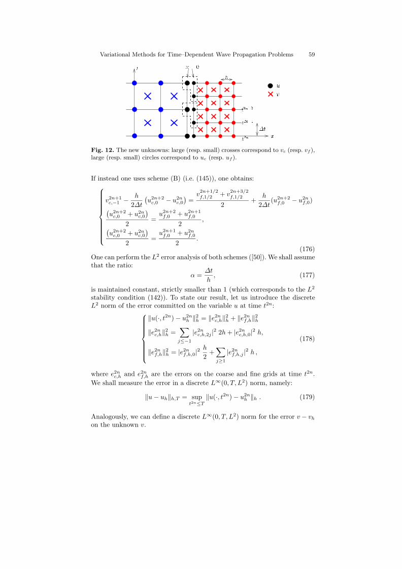
Variational Methods for Time–Dependent Wave Propagation Problems 59
u
t
v
t2n+1
t2n+2
t
x = 0
h
t2nx
Fig. 12. The new unknowns: large (resp. small) crosses correspond to vc (resp. vf ),large (resp. small) circles correspond to uc (resp. uf ).
If instead one uses scheme (B) (i.e. (145)), one obtains:
v2n+1c,−1 − h
2∆t
(u2n+2
c,0 − u2nc,0
)=
v2n+1/2f,1/2 + v
2n+3/2f,1/2
2+
h
2∆t(u2n+2
f,0 − u2nf,0)(
u2n+2c,0 + u2n
c,0
)2
=u2n+2
f,0 + u2n+1f,0
2,(
u2n+2c,0 + u2n
c,0
)2
=u2n+1
f,0 + u2nf,0
2.
(176)One can perform the L2 error analysis of both schemes ([50]). We shall assumethat the ratio:
α =∆t
h, (177)
is maintained constant, strictly smaller than 1 (which corresponds to the L2
stability condition (142)). To state our result, let us introduce the discreteL2 norm of the error committed on the variable u at time t2n:
‖u(·, t2n) − u2nh ‖2
h = ‖e2nc,h‖2
h + ‖e2nf,h‖2
h
‖e2nc,h‖2
h =∑
j≤−1
|e2nc,h,2j |2 2h + |e2n
c,h,0|2 h,
‖e2nf,h‖2
h = |e2nf,h,0|2
h
2+
∑j≥1
|e2nf,h,j |2 h ,
(178)
where e2nc,h and e2n
f,h are the errors on the coarse and fine grids at time t2n.We shall measure the error in a discrete L∞(0, T, L2) norm, namely:
‖u − uh‖h,T = supt2n≤T
‖u(·, t2n) − u2nh ‖h . (179)
Analogously, we can define a discrete L∞(0, T, L2) norm for the error v − vh
on the unknown v.
60 Patrick Joly
Theorem 2. Assume that the exact solution (u, v) has the regularity:
(u, v) ∈ C3(0, T ;L2), (180)
then with scheme (B), one has the error estimate:
‖u − uh‖h,T + ‖v − vh‖h,T ≤ C (1 − α2)−1/2 h1/2 ‖(u, v)‖C3(0,T ;L2). (181)
Assume that the exact solution (u, v) has the regularity:
(u, v) ∈ C3+k(0, T ;L2), k ≥ 0, (182)
then with scheme (A), one has the error estimate:
‖u − uh‖h,T + ‖v − vh‖h,T ≤ Ck (1 − α2)−1/2 hpk ‖(u, v)‖C3(0,T ;L2) (183)
where pk = 3/2 − 1/2k.
It is interesting to complete this result with some comments.
– The proof of this theorem is not completely standard. Let us give themain ideas. The errors u − uh and v − vh satisfy the same interior andtransmission schemes as uh and vh except that truncation errors appear atthe right hand sides:– an interior truncation error which is O(h2)– an interface truncation error, which is located at the numerical interface
and is O(h), due to the off-centred nature of the discrete transmissionconditions (175) or (176).
Thus a priori we expect an O(h) error estimate. However, in order to applythe same type of energy analysis as in Sect. 2.4, and more particularly tohandle the interface truncation error, we have to use some kind of discretetrace estimate, typically:
|u2nc,0| ≤ h−1/2 ‖u2n
c,h‖h . (184)
This drops an additional half power of h in the estimate obtained by theenergy analysis which thus provides (for both schemes):
‖u − uh‖h,T + ‖v − vh‖h,T = O(h1/2). (185)
The proof stops here with scheme (176) for which it can be proven thatthe O(h1/2) estimate is optimal (see the next item). With scheme (175),one can improve the estimate thanks to a boot strap argument (this isthe most delicate point) which exploits the precise nature of the interfacetruncation error associated with scheme (175). One can show (more detailswill be given in [50]) that, if (u, v) ∈ C3+k(0, T ;L2):
‖u−uh‖h,T +‖v−vh‖h,T = O(hpk−1) =⇒ ‖u−uh‖h,T +‖v−vh‖h,T = O(hpk),(186)
where pk = 1/2 pk−1 + 3/4 which yields pk = 3/2 − 1/2k.
Variational Methods for Time–Dependent Wave Propagation Problems 61
– Passing from a discrete L∞(0, T ;L2) norm to an L∞(0, T ;L∞), one loosesone half power of h in the error estimates. This means that the method isfirst order accurate in L∞ with scheme (175), but that maybe not conver-gent in L∞ with scheme (176). This is in fact clearly the case since, from(176), one deduces in particular that:
u2n+2c,0 = u2n
c,0,
In other words the trace on the interface of the coarse grid solution isconstant at even instants (which is, of course, not the case of the exactsolution). This also shows the optimality of the O(h1/2) L2-estimate forscheme (176)
– The result of the theorem essentially says that the method is of order 1/2with scheme (176) and of order 3/2 (take k arbitrarily large in (183)) withscheme (175). In both cases, one loses some accuracy with respect to theinterior scheme which is second order accurate. A challenging and still openquestion is to find more accurate conservative transmission schemes.
– The constants appearing in the error estimates (181) and (183) blow upwhen α tends to 1, similarly to what we obtain with the estimate (58) (seeSect. 2.4 and remark 10). It is not possible here to improve the result byapplying a technique similar to the one that we presented in the remark 10:indeed, due to the change of time step between the two grids, the schemeis not invariant by translation of ∆t. Moreover, the numerical experimentsindicate that the method is not strongly convergent when α = 1 (however,we conjecture that, in this case, the discrete solution converges weakly inL2 to the continuous one).
– In [30], we made a different analysis which completes (and some how con-firms) the results of Theorem 2. This analysis consists of looking at whathappens to an incident harmonic wave of amplitude 1 and frequency ω inthe coarse grid. This incident wave gives rise to:– a reflected wave of frequency ω and amplitude R in the fine grid.– a transmitted wave of frequency ω and amplitude T in the fine grid.– a parasitic transmitted wave of frequency ω+π/∆t in the fine grid. This
wave is evanescent, i.e. exponentially decaying with the distance to theinterface, and has an amplitude T ′ on the interface. The penetrationdepth is proportional to h.
Remark 23. The existence of the high frequency parasitic wave is due tothe so-called aliasing phenomenon: the two frequencies ω are ω +π/∆t are“equal” for the coarse grid but distinct for the fine grid.
An asymptotic analysis for small h shows that:– With scheme (175), R = 0(h2), T = 1 − 0(h2), T ′ = 0(h).– With scheme (176), R = 0(h2), T = 1 − 0(h2), T ′ = 0(1).This illustrates once again the superiority of scheme (175) (or scheme (A))with respect to scheme (176) (or scheme (B)). It also confirms in some
62 Patrick Joly
sense the optimality of the estimates (181) and (183). Roughly speaking,the amplitude of the parasitic wave is a function of the form (γ is a givenpositive constant):
T ′ exp(− γx
h), x > 0,
and the L2 norm of such a function is equal to |T ′|√
h/γ which givesO(h1/2) with scheme (176) and O(h3/2) with scheme (175).
Acknowledgements. I would like to thank my collaborators Eliane Becache,Gary Cohen, Francis Collino, Julien Diaz, Gregoire Derveaux, Thierry Fou-quet, Sylvain Garces, Florence Millot, Leila Rhouti, Jeronimo Rodriguez,Chrysoula Tsogka for their collaboration and their essential contributions tosome of the works presented in this article. I also thank particularly JeronimoRodriguez and Houssem Haddar for their careful reading of the manuscriptand the improvements they have proposed.
References
1. D.N. Arnold, F. Brezzi and J. Douglas. PEERS: A new mixed finite elementfor plane elasticity. Japan J. Appl. Math., 1:347–367, 1984.
2. G.P. Astrakmantev. Methods of fictitious domains for a second order ellipticequation with natural boundary conditions. U.S.S.R Comp. Math. and Math.Phys., 18:114–221, 1978.
3. C. Atamian, R. Glowinski, J. Periaux, H. Steve and G. Terrason. Con-trol approach to fictitious domain in electro-magnetism. Conference surl’approximation et les methodes numeriques pour la resolution des equationsde Maxwell, Hotel Pullmann, Paris, 1989.
4. C. Atamian and P. Joly. An analysis of the method of fictitious domains for theexterior Helmholtz problem. RAIRO Model. Math. Anal. Numer, 27(3):251–288, 1993.
5. I. Babuska. The Finite Element Method with Lagrangian Multipliers. Numer.Math., 20:179–192, 1973.
6. G.A. Baker and V.A. Dougalis. The Effect of Quadrature Errors on FiniteElement Approximations for the Second-Order Hyperbolic Equations. SIAM.Journ. Numer. Anal., 13(4):577–598, 1976.
7. A. Bamberger, R. Glowinski and Q. H. Tran. A domain decomposition methodfor the acoustic wave equation with discontinuous coefficients and grid change.SIAM J. on Num. Anal., 34(2):603–639, April 1997.
8. E. Becache, P. Joly and G. Scarella. A fictitious domain method for unilateralcontact problems in non destructive testing. In Computational and Fluid ansSolid Mechanics, pages 65–67, 2001.
9. E. Becache, P. Joly and C. Tsogka. An analysis of new mixed finite elementsfor the approximation of wave propagation problems. SIAM J. Numer.Anal.,37(4):1053–1084, 2000.
Variational Methods for Time–Dependent Wave Propagation Problems 63
10. E. Becache, P. Joly and C. Tsogka. Fictitious domains, mixed FE and PMLfor 2-D elastodynamics. Journal of Computational Acoustics, 9(3):1175–1201,2001.
11. E. Becache, P. Joly and C. Tsogka. A new family of mixed finite elementsfor the linear elastodynamic problem. SIAM J. Numer.Anal., 39(6):2109–2132,2002.
12. F. Ben Belgacem. The mortar finite element method with Lagrange multipliers.Numer. Math., 84(2):173–197, 1999.
13. F. Ben Belgacem, A. Buffa and Y. Maday. The mortar finite element methodfor 3d maxwell equations: First results. SIAM J. Numer. Anal., 39(3):880–901,2001.
14. A. Bendali. Approximation par elements finis de surface de problemes dediffraction des ondes electromagnetiques. PhD thesis, Universite Paris VI, 1984.
15. C. Bernardi and Y. Maday. Raffinement de maillage en elements finis par lamethode des joints. C. R. Acad. Sci. Paris Ser. I Math., 320(3):373–377, 1995.
16. F. Brezzi and M. Fortin. Mixed and Hybrid Finite Element Methods. SpringerSeries in Computational Mathematics (15). Springer Verlag, 1991.
17. A. Buffa and P. Ciarlet Jr. On traces for functional spaces related to Maxwell’sequations. I. an integration by parts formula in Lipschitz polyhedra. Mathe-matical Methods in the Applied Sciences, 24(1):9–30, 2001.
18. A. Chaigne, P. Joly and L. Rhaouti. Time-domain modeling and numerical sim-ulation of a kettledrum. Journal of the Acoustical Society of America, 6:3545–3562, 1999.
19. M.W. Chevalier and R.J. Luebbers. FDTD local grid with material traverse.IEEE Transactions on Antennas and Propagation, 45(3):411–421, March 1997.
20. M.J.S. Chin-Joe-Kong, W.A. Mulder and M. Van Veldhuizen. Higher-ordertriangular and tetrahedral finite elements with mass lumping for solving thewave equation. J. Engrg. Math., 35(4):405–426, 1999.
21. P.G. Ciarlet. The finite element method for elliptic problems. Reprinted bySIAM in 2002, original by North-Holland, 1982.
22. M. Clemens, P. Thoma, T. Weiland and U. van Rienen. Computationalelectromagnetic-field calculation with the finite-integration method. SurveysMath. Indust., 8(3-4):213–232, 1999.
23. P. Clement. Approximation by finite element functions using local regulariza-tion. Rev. Fran. Automat. Informat. Rech. Oper. Ser. Rouge Anal. Numer.,9:77–84, 1975.
24. G. Cohen. Higher-order numerical methods for transient wave equations. Sci-entific Computation, 2002.
25. G. Cohen, P. Joly and N. Torjman. Higher-order finite elements with mass-lumping for the 1D wave equation. Finite Elements in Analysis and Design,16:329–336, 1994.
26. G. Cohen, P. Joly, N. Torjman and J. Roberts. Higher order triangular finiteelements with mass lumping for the wave equation. SIAM J. Numer. Anal.,38(6):2047–2078, 2001.
27. G. Cohen and P. Monk. Gauss point mass lumping schemes for Maxwell’sequations. Numer. Methods Partial Differential Equations, 14(1):63–88, 1998.
28. G. Cohen and P. Monk. Mur-Nedelec finite element schemes for Maxwell’sequations. Comput. Methods Appl. Mech. Engrg., 169(3-4):197–217, 1999.
64 Patrick Joly
29. F. Collino, P. Joly and T. Fouquet. A Conservative Space-time Mesh Refine-ment Method for the 1-D Wave Equation. Part I : Construction. Num. Math.,To appear.
30. F. Collino, P. Joly and T. Fouquet. A Conservative Space-time Mesh Refine-ment Method for the 1-D Wave Equation. Part II : Analysis. Num. Math., Toappear.
31. F. Collino, P. Joly and S. Garces. A fictitious domain method for conformalmodeling of the perfect electric conductors in the FDTD method. IEEE Trans.on Antennas and Propagation, 46:1519–1527, 1997.
32. F. Collino, P. Joly and F. Millot. Fictitious domain method for unsteadyproblems: Application to electromagnetic scattering. Journal of Comp. Physics,138:907–938, 1997.
33. G. Derveaux. Modelisation Numerique de la Guitare Acoustique. PhD thesis,Ecole Polytechnique , 2002.
34. T. Dupont. L2 estimates or Galerkin methods for second-order hyperbolicequations. SIAM J. Numer.Anal., 10:880–889, 1973.
35. A. Elmkies. Elements finis et condensation de masse pour les equations deMaxwell. PhD thesis, Universite Paris XI, Orsay, June 1998.
36. A. Elmkies and P. Joly. Elements finis et condensation de masse pour lesequations de Maxwell : le cas 2D. C.R. Acad. Sci. Paris, t. 324(Serie I):1287–1292, 1997.
37. A. Elmkies and P. Joly. Elements finis et condensation de masse pour lesequations de Maxwell : le cas 3D. C.R. Acad. Sci. Paris, t. 325(Serie I):1217–1222, 1997.
38. B. Engquist and A. Majda. Absorbing boundary conditions for the numericalsimulation of waves. Math. of Comp., 31:629–651, 1977.
39. S.A Finogenov and Y.A. Kuznetsov. Two stage fictitious components methodsfor solving the Dirichlet boundary value problem. Sov. J. Num. Anal. Math.Modelling, 3:301–323, 1988.
40. G.J. Fix. Effects of quadrature errors in finite element approximation of steadystate, eigenvalue and parabolic problems. In The Mathematical Fondations ofthe Finit Element Method with Applications to Partial Differential Equations,pages 525–556, 1972.
41. T. Fouquet. Raffinement de maillage spatio-temporel pour les equations deMaxwell. PhD thesis, Universite Paris IX Dauphine, June 2000.
42. S. Garces. Application des methodes de domaines fictifs a la modelisation desstructures rayonnantes tridimensionnelles Etude mathematique et numeriqued’un modele. PhD thesis, ENSAE (Toulouse) , 1997.
43. T. Geveci. On the application of mixed finite element methods to the waveequations. RAIRO Model. Math. Anal. Numer., 22(2):243–250, 1988.
44. V. Girault and R. Glowinski. Error analysis of a fict. domain method appliedto a Dirichlet problem. Japan J. Ind. Appl. Math., 12(3):487–514, 1995.
45. R. Glowinski, T.W. Pan, and J. Periaux. A fictitious domain method for Dirich-let problem and applications. Comp. Meth. in Appl. Mech. and Eng., 111:283–303, 1994.
46. R. Glowinski, T.W. Pan and J. Periaux. A fictitious domain method for externalincompressible viscous flow modeled by Navier-Stokes equations. Comp. Meth.Appl. Mech. Eng., 112:133–148, 1994.
Variational Methods for Time–Dependent Wave Propagation Problems 65
47. P. Have, M. Kern and C. Lemuet. Resolution numerique de l’equation desondes par une methode d’elements finis d’ordre eleve sur calculateur parallele.Technical Report 4381, I.N.R.I.A., Fevrier 2002.
48. P. Joly and C. Poirier. A new second order edge element on tetrahedra fortime dependent maxwell’s equations. In Mathematical and Numerical Aspectsof Wave Propagation, pages 842–847, 2000.
49. P. Joly and L. Rhaouti. Domaines fictifs, elements finis h(div) et condition deneumann: le probleme de la condition inf-sup. C. R. Acad. Sci. Paris, Serie I,328:1225–1230, 1999.
50. P. Joly and J. Rodriguez. l2 error analysis of space-time mesh refinementschemes for the 1d wave equation. in preparation.
51. I. S. Kim and W. J. R. Hoefer. A local mesh refinement algorithm for the time-domain finite-difference method to solve maxwell’s equations. IEEE Trans.Microwave Theory Tech., 38(6):812–815, June 1990.
52. K.S. Kunz and L. Simpson. A technique for increasing the resolution of finite-difference solutions to the maxwell equations. IEEE Trans. Electromagn. Com-pat., EMC-23:419–422, Nov. 1981.
53. J.L. Lions and E. Magenes. Problemes aux Limites non Homogenes et Appli-cations. Dunod, 1968.
54. Ch.G. Makridakis. On mixed finite element methods for linear elastodynamics.Numer. Math., 61(2):235–260, 1992.
55. G.I. Marchuk, Y.A. Kuznetsov and A.M. Matsokin. Fictitious domain anddomain decomposition methods. Sov. J. Num. Anal. Math. Modelling, 1:3–35,1986.
56. P. Monk. Analysis of a finite element method for Maxwell’s equations. SIAMJ. Numer.Anal., 29(3):714–729, 1992.
57. P. Monk. Sub-gridding FDTD schemes. ACES Journal, 11:37–46, 1996.58. P. Monk and O. Vacus. Error estimates for a numerical scheme for ferromag-
netic problems. SIAM J. Numer.Anal., 36(3):696–718, 1999.59. J.C. Nedelec. Mixed finite elements in IR3. Num. Math., 35:315–341, 1980.60. J.C. Nedelec. A new family of mixed finite elements in IR3. Num. Math.,
50:57–81, 1986.61. V. Petkov. Scattering theory for hyperbolic operators. Studies in Mathematics
and its Applications, 1989.62. S. Piperno, M. Remaki and L. Fezoui. A nondiffusive finite volume scheme for
the three-dimensional Maxwell’s equations on unstructured meshes. SIAM J.Numer. Anal., 9(6):2089–2108, 2002.
63. D.T. Prescott and N.V. Shuley. A method for incorporating different sizedcells into the finite-difference time-domain analysis technique. IEEE MicrowaveGuided Wave Lett., 2:434–436, Nov. 1992.
64. P.A. Raviart. The use of numerical integration in finite element methods forparabolic equations. In Topics in Numerical Analysis Proc., pages 233–264,1973.
65. A. Taflove. Computational Electrodynamics, The Finite-Difference Time Do-main method. Artech House, London, 1995.
66. A. Ben Haj Yedder, E. Becache, P. Joly and A. Komech. A fictitious domainapproach to the scattering of waves by mobile obstacles. in preparation.
67. K.S. Yee. Numerical solution of initial boundary value problems involvingMaxwell’s equations in isotropic media. IEEE Trans. on Antennas and propa-gation, pages 302–307, 1966.
![LAWRENCE LIVERMORE NATIONAL LABORATORY Wave … · an isotropic material can lead to directionally dependent wave propagation properties [2], i.e., anisotropic behavior. More generally,](https://img.pdfslide.us/doc/110x75/5f6c5c48041bbf414967cfef/lawrence-livermore-national-laboratory-wave-an-isotropic-material-can-lead-to-directionally.jpg)


![Experimental Study on Shape Dependent Wave Force of ... · force was dependent on the support structure shape, wave height, and ... (Gravity Base System) [7], [8], Hybrid (1), and](https://img.pdfslide.us/doc/110x75/5fd18f148064ef430234ef0a/experimental-study-on-shape-dependent-wave-force-of-force-was-dependent-on-the.jpg)