Variational data assimilation for very large environmental ... · simple interpolation between the observations and the model state, ... Over the following decade many ... These two

Variational data assimilation for very large environmental problems Book or Report Section

Accepted Version

Lawless, A. (2013) Variational data assimilation for very large environmental problems. In: Cullen, M., Freitag, M.A., Kindermann, S. and Scheichl, R. (eds.) Large Scale Inverse Problems: Computational Methods and Applications in the Earth Sciences. Radon Series on Computational and Applied Mathematics , 2 (13). De Gruyter, Berlin, pp. 5590. ISBN 9783110282269 Available at http://centaur.reading.ac.uk/37707/

It is advisable to refer to the publisher’s version if you intend to cite from the work. Published version at: http://www.degruyter.com/view/product/182025

Publisher: De Gruyter

All outputs in CentAUR are protected by Intellectual Property Rights law, including copyright law. Copyright and IPR is retained by the creators or other copyright holders. Terms and conditions for use of this material are defined in the End User Agreement .

www.reading.ac.uk/centaur

http://centaur.reading.ac.uk/licence

http://www.reading.ac.uk/centaur

CentAUR

Central Archive at the University of Reading

Reading’s research outputs online

XXXX, 1–37 © De Gruyter YYYY

Variational data assimilation for very largeenvironmental problems

Amos S. Lawless

Abstract. Variational data assimilation is commonly used in environmental forecasting to es-timate the current state of the system from a model forecast and observational data. The as-similation problem can be written simply in the form of a nonlinear least squares optimizationproblem. However the practical solution of the problem in large systems requires many carefulchoices to be made in the implementation. In this article we present the theory of variationaldata assimilation and then discuss in detail how it is implemented in practice. Current solutionsand open questions are discussed.

Keywords. 3D-Var, 4D-Var, adjoint model, background errors, error covariance, incrementalformulation, nested models, observation errors, optimization, reduced order models, tangentlinear model, weak-constraint.

AMS classification. 49-02, 65-02, 86-02.

1 Introduction

Data assimilation is the process of combining a numerical model forecast with ob-servational data in order to estimate the current state of a dynamical system. It hasbeen an essential part of numerical weather prediction (NWP) since its beginnings inthe 1940s, when it was recognized that errors in the initial model state could rapidlylead to large errors in the forecast. Early data assimilation schemes were based on asimple interpolation between the observations and the model state, with later schemesalso taking account of the statistics of the errors in the data. Such schemes includedsmoothing splines, successive correction, optimal interpolation and analysis correction[82], [85]. The possible use of methods based on variational calculus was proposed bySasaki [103], [104] in the late 1950s and 1960s, but at the time a practical implemen-tation was not possible. A real breakthrough in the application of variational schemesto NWP came in the late 1980s with a series of papers demonstrating how the prob-lem could be solved using techniques from the theory of optimal control, in particularthe use of adjoint equations to calculate the gradient of an objective function, or cost

The author is supported in part by the U.K. Natural Environment Research Council, through the NationalCentre for Earth Observation.To appear in Large Scale Inverse Problems: Computational Methods and Applications in the Earth Sci-ences (2013), Eds. Cullen, M.J.P., Freitag, M. A., Kindermann, S., Scheichl, R., Radon Series on Com-putational and Applied Mathematics 13.

2 A. S. Lawless

function [77], [107]. This led to a series of papers in which the feasibility of vari-ational data assimilation was studied on a series of different simplified atmosphericmodels [108], [98], [26], [93] (these experiments usually only included the large-scaleatmospheric dynamics and not the subgrid-scale processes of full weather predictionmodels).

Despite the encouraging results of these experiments variational data assimilationremained impractical for operational use due to the high computational cost. Theintroduction of the incremental method of variational assimilation in 1994 [27], to-gether with increasing computing power, opened up the possibility of an affordableimplementation for operational weather prediction. Over the following decade manyweather forecasting centres began to develop variational data assimilation for opera-tional use [99], [84], [100], [42], [43], [61]. At the same time variational data assimi-lation began to be applied to other applications, such as ocean forecasting [116], [112]and atmospheric chemistry [38].

A common feature of many of these applications is that the size of the state variablebeing estimated is extremely large. Current numerical weather prediction models mayrequire the initialization of the order of 108 variables in order to make a forecast.As computing power increases the spatial resolution of the models tends to increaseand hence so does the number of variables being represented. Furthermore the real-time nature of environmental forecasting requires that the data assimilation problembe solved quickly. These two factors imply that when implementing variational dataassimilation schemes in practice compromises must be made. Hence it is importantto design the algorithms carefully to ensure that as accurate a solution as possible isobtained within the time available. Ideally such design should also include knowledgeof the physics of the problem, so that the final solution is physically realistic. In theremainder of this article we will discuss some of the different choices that arise in theimplementation of variational data assimilation for very large systems and the practicalapproaches that have been developed. First we briefly present the mathematical theoryof variational data assimilation.

2 Theory of variational data assimilation

We consider a discrete nonlinear dynamical system given by the equation

xi+1 =Mi(xi), (2.1)

where xi ∈ Rn is the state vector at time ti andMi is the nonlinear model operatorthat propagates the state at time ti to time ti+1 for i = 0, 1, . . . , N − 1. We assumethat we have imperfect observations yi ∈ Rpi at times ti, i = 0, . . . , N that are relatedto the system state through the equation

yi = Hi(xi) + εi, (2.2)

Variational data assimilation 3

where Hi : Rn → Rpi is known as the observation operator and maps the state vectorto observation space. The observation errors εi are usually assumed to be unbiased,serially uncorrelated, Gaussian errors with known covariance matrices Ri. For thenumerical weather prediction problem the vector xi would contain several meteoro-logical variables, such as pressure, temperature and the three-dimensional wind, ateach grid point of the model domain. The observation operator Hi may just be a sim-ple interpolation in space, if the state variable is observed directly. However, it couldbe a much more complicated nonlinear function of the state. For example, for a satel-lite radiance measurement the observation operator can include a complex radiativetransfer model.

We assume that at the initial time t0 we have an a priori estimate of the state, usuallyreferred to as a background field, that we denote xb. This background field is assumedto have unbiased, Gaussian errors with known covariance matrix B. In practice thebackground field is usually a short-term forecast of the state from a previous assimi-lation cycle. The problem of four-dimensional variational data assimilation (4D-Var)1

is then to find the initial state that minimizes the weighted least squares distance tothis background while minimizing the weighted least squares distance of the modeltrajectory to the observations over the time interval [t0, tN ]. Mathematically we canformulate this as an optimization problem:Find the state xa0 at time t0 that minimizes the function

J (x0) =12(x0−xb)TB−1(x0−xb)+

12

N∑i=0

(Hi(xi)−yi)TR−1i (Hi(xi)−yi) (2.3)

subject to the states xi satisfying the nonlinear dynamical system (2.1). In the casewhere N = 0 there is no model evolution and the scheme is referred to as three-dimensional variational data assimilation (3D-Var). The solution xa0 is commonly re-ferred to as the analysis. In environmental data assimilation the function J (x0) isusually called the cost function, but the terms objective function and penalty functionare often used in other fields.

The minimization problem given by equation (2.3) can be interpreted in a statisti-cal or deterministic sense. From Bayes’ theorem it can be shown that xa0 gives themaximimum a posteriori estimate of the state under the assumptions given [82]. Thisincludes the assumption of Gaussianity of the error statistics for the background fieldand observations. In practice this assumption may not always hold. For example, forvariables that are inherently non-negative, such as humidity in the atmosphere or con-centrations in chemical models, Gaussian statistics may not be appropriate. In somecases these errors may be treated by assuming a lognormal distribution and using thisto transform to variables whose statistics are Gaussian [13], [41]. Some allowance fornon-Gaussian observation errors may also be made using the method of variational

1 The scheme is referred to as four-dimensional since we usually fit three spatial dimensions in time,with time being the fourth dimension.

4 A. S. Lawless

quality control, as discussed in section 3.3. Furthermore, nonlinearity in the dynam-ical model implies that the background errors are likely to be non-Gaussian if thebackground comes from a forecast whose length is beyond the linearity regime of themodel. For this reason in numerical weather prediction the background field is usuallyfrom a forecast of only 6 or 12 hours. In some applications, such as the identificationof the source of an atmospheric tracer, it may be more appropriate to specify otherprior error distributions [12]. The alternative, deterministic interpretation of the mini-mization problem is to consider the term measuring the fit to the background state asa form of Tikhonov regularization in fitting the observations [65], [29], [90]. Each ofthese interpretations is able to provide different insights into the practical formulationof the problem.

It is instructive to consider the solution to the 3D-Var problem under the hypothesisthat the observation operatorH0 is approximately linear, such that

H0(xb)−H0(x0) ≈ H0(xb)(xb − x0) (2.4)

where H0(xb) is the Jacobian ofH0 evaluated at xb (This assumption (2.4) is referredto as the tangent linear hypothesis). In this case the minimum value of (2.3) can bewritten explicitly as

xa = xb + BHT0 (H0BHT

0 + R0)−1(y0 −H0(xb)). (2.5)

This solution is equal to the best linear unbiased estimate (or BLUE). We see thenthat the analysis increment, defined as the difference between the analysis and thebackground xa−xb, lies in the range space of the background error covariance matrixB. We return to the implications of this in section 3.2.

The covariance of the analysis error in this case is given by

A = (B−1 + HT0 R−1

0 H0)−1. (2.6)

We find that for both 3D-Var and 4D-Var this is equal to the inverse of the Hessian ofthe cost function,

A = (∇2J )−1. (2.7)

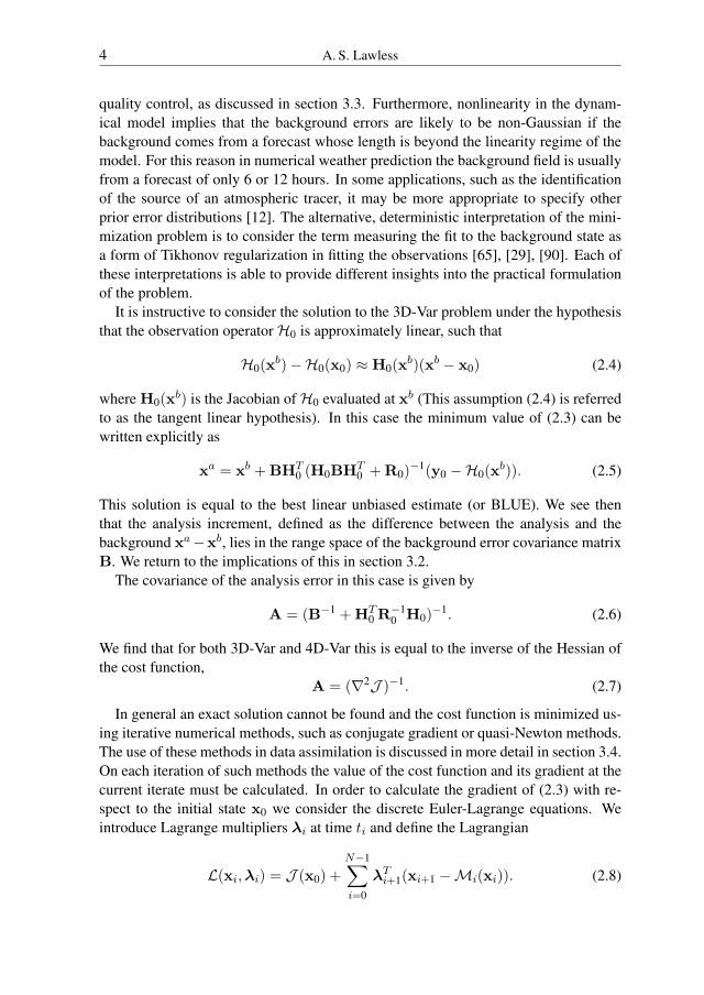
In general an exact solution cannot be found and the cost function is minimized us-ing iterative numerical methods, such as conjugate gradient or quasi-Newton methods.The use of these methods in data assimilation is discussed in more detail in section 3.4.On each iteration of such methods the value of the cost function and its gradient at thecurrent iterate must be calculated. In order to calculate the gradient of (2.3) with re-spect to the initial state x0 we consider the discrete Euler-Lagrange equations. Weintroduce Lagrange multipliers λi at time ti and define the Lagrangian

L(xi,λi) = J (x0) +N−1∑i=0

λTi+1(xi+1 −Mi(xi)). (2.8)


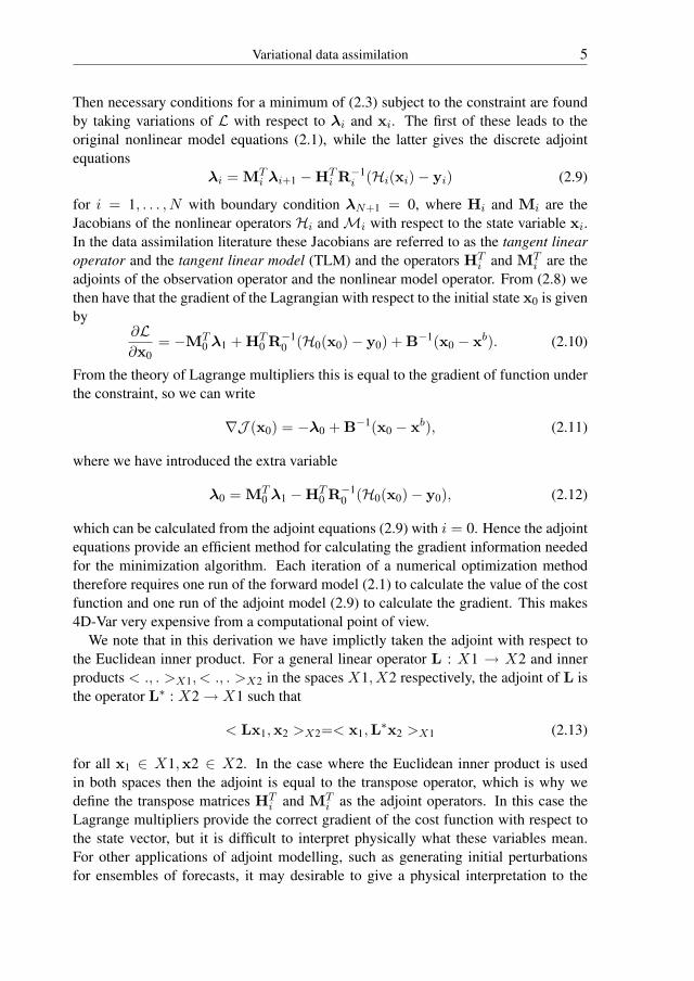
Then necessary conditions for a minimum of (2.3) subject to the constraint are foundby taking variations of L with respect to λi and xi. The first of these leads to theoriginal nonlinear model equations (2.1), while the latter gives the discrete adjointequations

λi = MTi λi+1 −HT

i R−1i (Hi(xi)− yi) (2.9)

for i = 1, . . . , N with boundary condition λN+1 = 0, where Hi and Mi are theJacobians of the nonlinear operators Hi andMi with respect to the state variable xi.In the data assimilation literature these Jacobians are referred to as the tangent linearoperator and the tangent linear model (TLM) and the operators HT

i and MTi are the

adjoints of the observation operator and the nonlinear model operator. From (2.8) wethen have that the gradient of the Lagrangian with respect to the initial state x0 is givenby

∂L∂x0

= −MT0 λ1 + HT

0 R−10 (H0(x0)− y0) + B−1(x0 − xb). (2.10)

From the theory of Lagrange multipliers this is equal to the gradient of function underthe constraint, so we can write

∇J (x0) = −λ0 + B−1(x0 − xb), (2.11)

where we have introduced the extra variable

λ0 = MT0 λ1 −HT

0 R−10 (H0(x0)− y0), (2.12)

which can be calculated from the adjoint equations (2.9) with i = 0. Hence the adjointequations provide an efficient method for calculating the gradient information neededfor the minimization algorithm. Each iteration of a numerical optimization methodtherefore requires one run of the forward model (2.1) to calculate the value of the costfunction and one run of the adjoint model (2.9) to calculate the gradient. This makes4D-Var very expensive from a computational point of view.

We note that in this derivation we have implictly taken the adjoint with respect tothe Euclidean inner product. For a general linear operator L : X1 → X2 and innerproducts < ., . >X1, < ., . >X2 in the spaces X1, X2 respectively, the adjoint of L isthe operator L∗ : X2→ X1 such that

< Lx1,x2 >X2=< x1,L∗x2 >X1 (2.13)

for all x1 ∈ X1,x2 ∈ X2. In the case where the Euclidean inner product is usedin both spaces then the adjoint is equal to the transpose operator, which is why wedefine the transpose matrices HT

i and MTi as the adjoint operators. In this case the

Lagrange multipliers provide the correct gradient of the cost function with respect tothe state vector, but it is difficult to interpret physically what these variables mean.For other applications of adjoint modelling, such as generating initial perturbationsfor ensembles of forecasts, it may desirable to give a physical interpretation to the

6 A. S. Lawless

gradients calculated from the Lagrange multipliers. In these applications other innerproducts may be used, for example based on the energy or enstrophy2 of the system[95].

2.1 Incremental variational data assimilation

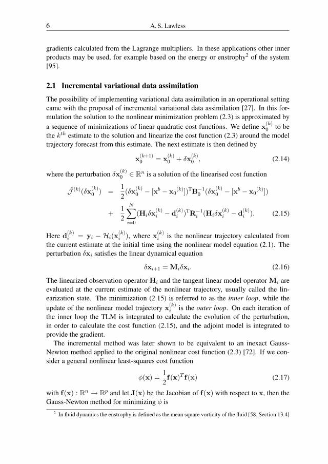
The possibility of implementing variational data assimilation in an operational settingcame with the proposal of incremental variational data assimilation [27]. In this for-mulation the solution to the nonlinear minimization problem (2.3) is approximated bya sequence of minimizations of linear quadratic cost functions. We define x(k)

0 to bethe kth estimate to the solution and linearize the cost function (2.3) around the modeltrajectory forecast from this estimate. The next estimate is then defined by

x(k+1)0 = x(k)

0 + δx(k)0 , (2.14)

where the perturbation δx(k)0 ∈ Rn is a solution of the linearised cost function

J (k)(δx(k)0 ) =

12(δx(k)

0 − [xb − x0(k)])TB−1

0 (δx(k)0 − [xb − x0

(k)])

+12

N∑i=0

(Hiδx(k)i − d(k)

i )TR−1i (Hiδx

(k)i − d(k)

i ). (2.15)

Here d(k)i = yi − Hi(x(k)

i ), where x(k)i is the nonlinear trajectory calculated from

the current estimate at the initial time using the nonlinear model equation (2.1). Theperturbation δxi satisfies the linear dynamical equation

δxi+1 = Miδxi. (2.16)

The linearized observation operator Hi and the tangent linear model operator Mi areevaluated at the current estimate of the nonlinear trajectory, usually called the lin-earization state. The minimization (2.15) is referred to as the inner loop, while theupdate of the nonlinear model trajectory x(k)

i is the outer loop. On each iteration ofthe inner loop the TLM is integrated to calculate the evolution of the perturbation,in order to calculate the cost function (2.15), and the adjoint model is integrated toprovide the gradient.

The incremental method was later shown to be equivalent to an inexact Gauss-Newton method applied to the original nonlinear cost function (2.3) [72]. If we con-sider a general nonlinear least-squares cost function

φ(x) =12f(x)T f(x) (2.17)

with f(x) : Rn → Rp and let J(x) be the Jacobian of f(x) with respect to x, then theGauss-Newton method for minimizing φ is

2 In fluid dynamics the enstrophy is defined as the mean square vorticity of the fluid [58, Section 13.4]


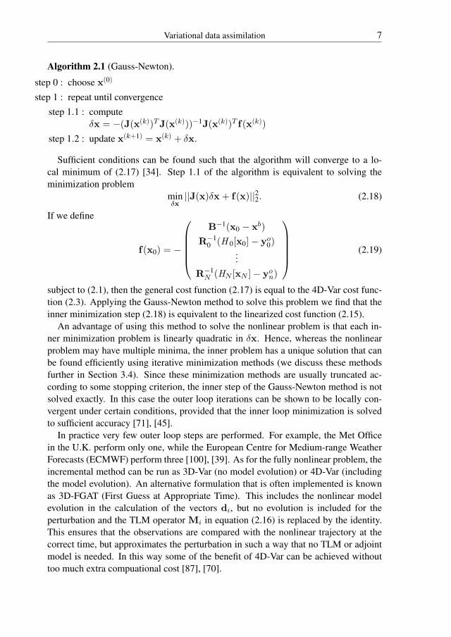
Algorithm 2.1 (Gauss-Newton).

step 0 : choose x(0)

step 1 : repeat until convergence

step 1.1 : computeδx = −(J(x(k))TJ(x(k)))−1J(x(k))T f(x(k))

step 1.2 : update x(k+1) = x(k) + δx.

Sufficient conditions can be found such that the algorithm will converge to a lo-cal minimum of (2.17) [34]. Step 1.1 of the algorithm is equivalent to solving theminimization problem

minδx||J(x)δx + f(x)||22. (2.18)

If we define

f(x0) = −

B−1(x0 − xb)

R−10 (H 0[x0]− yo0)

...R−1N (HN [xN ]− yon)

(2.19)

subject to (2.1), then the general cost function (2.17) is equal to the 4D-Var cost func-tion (2.3). Applying the Gauss-Newton method to solve this problem we find that theinner minimization step (2.18) is equivalent to the linearized cost function (2.15).

An advantage of using this method to solve the nonlinear problem is that each in-ner minimization problem is linearly quadratic in δx. Hence, whereas the nonlinearproblem may have multiple minima, the inner problem has a unique solution that canbe found efficiently using iterative minimization methods (we discuss these methodsfurther in Section 3.4). Since these minimization methods are usually truncated ac-cording to some stopping criterion, the inner step of the Gauss-Newton method is notsolved exactly. In this case the outer loop iterations can be shown to be locally con-vergent under certain conditions, provided that the inner loop minimization is solvedto sufficient accuracy [71], [45].

In practice very few outer loop steps are performed. For example, the Met Officein the U.K. perform only one, while the European Centre for Medium-range WeatherForecasts (ECMWF) perform three [100], [39]. As for the fully nonlinear problem, theincremental method can be run as 3D-Var (no model evolution) or 4D-Var (includingthe model evolution). An alternative formulation that is often implemented is knownas 3D-FGAT (First Guess at Appropriate Time). This includes the nonlinear modelevolution in the calculation of the vectors di, but no evolution is included for theperturbation and the TLM operator Mi in equation (2.16) is replaced by the identity.This ensures that the observations are compared with the nonlinear trajectory at thecorrect time, but approximates the perturbation in such a way that no TLM or adjointmodel is needed. In this way some of the benefit of 4D-Var can be achieved withouttoo much extra compuational cost [87], [70].

8 A. S. Lawless

A major advantage of the incremental approach is that the inner loop minimizationproblem may be solved in a smaller dimensional space than the outer loop step, forexample at a lower spatial resolution. In this way the TLM and adjoint model needonly be run at the lower resolution on each inner loop iteration, while the linearizationtrajectory from the nonlinear model is still calculated at the higher resolution on eachouter loop. This is discussed further in Section 3.5. The computational savings madeby implementing the inner loop in this way made incremental 4D-Var feasible foroperational weather and ocean forecasting.

Having presented the basic theory of variational data assimilation we now examinesome of the issues that arise in its practical implementation. For the very large systemsfound in environmental modelling it is not always possible to apply the theory in anintuitive way. Many choices must be made in order to set up and solve the assimilationproblem efficiently and compromises must often be made. It is the attention to detailin these choices that can determine the success or otherwise of the data assimilationscheme.

3 Practical implementation

3.1 Model development

The development of a 4D-Var scheme for the large models used in operational weatherand ocean forecasting is a huge undertaking. In most cases the nonlinear model codealready exists and has been developed over many years. These models are very largepieces of software, with maybe close to one million lines of code. In order to developan incremental 4D-Var scheme the code for the TLM and adjoint model must first bewritten. The development of a TLM code and adjoint model code from the source codeof a nonlinear model is a fairly automatic procedure. The correct code for the TLM canbe found from a linearization of each statement of the nonlinear model source code,based on treating the nonlinear model as a series of arithmetic operations and apply-ing the chain rule. The adjoint model is then found by a line-by-line transpose of theTLM source code in reverse order. This method is known as automatic differentiation.We do not go into details of its application here, but refer the reader to several goodintroductions in the literature [26], [10], [102], [44]. The automatic nature of this pro-cedure has led to many software tools being developed that will produce a TLM andadjoint model code from a nonlinear mode source code. These automatic differentia-tion tools, or automatic adjoint compilers, are now available commercially for manydifferent programming languages. 3

In practice the TLM and adjoint models of many large environmental models havebeen developed by hand, rather than using the automatic compilers. There are sev-eral reasons for this. The first is that in many cases of operational weather and oceanforecasting the complexity of the already exisiting nonlinear model codes was such

3 The term automatic differentiation refers to the approach itself, not just to the automatic tools.


that simple application of the automatic compilers was not possible. In many cases,particularly for large codes developed by many people, it is necessary to tidy the non-linear model codes to make them suitable for use with the automatic compilers. Manycentres felt that the effort to do this would have been greater than coding the TLM andadjoint model by hand.

The second reason for developing the TLM and adjoint codes by hand arises fromthe nature of the incremental approach to variational data assimilation. Since the TLMand adjoint are run at a lower resolution in the inner loop, the TLM is already anapproximate linearization of the nonlinear model used in the outer loop. It is there-fore justifiable to make further simplifications in the TLM, in order to reduce thecomputational cost. As long as the adjoint model is derived from the approximateTLM, then the inner loop minimization will contain the correct gradient informationfor convergence. In coding the models by hand it is easier to make such simplifica-tions based on physical arguments. For example, many meteorological models containparametrizations of sub-grid-scale processes (known as the physics in the meteorolog-ical literature), which include such things as clouds, precipitation and surface drag.The schemes used to represent these processes can be highly complex and often in-clude non-differentiable functions, such as on-off switches. While it is possible forautomatic differentiation to deal with such functions it is usually felt that this level ofcomplexity is not necessary in the TLM and adjoint model. Hence a series of sim-pler parametrizations have been developed solely for use in incremental 4D-Var, thatcapture the main behaviour of the more complex schemes [118], [64], [99], [88].

An alternative approach, devised by the Met Office, is to start from the premise thatthe linear model must evolve finite and not infinitesimal perturbations and so there isno need for the linear model to be tangent to any nonlinear model. In this approachthe linear model is designed with this in mind. In particular, the resolved dynamics isapproximated by a discretization of the linearized continuous equations, with varioussimplifications in the equations and the discretization. Then simplified parametriza-tions can be used to represent sub-grid-scale processes [86], [74]. The adjoint modelis derived from this approximate linear model by the process of automatic differentia-tion, ensuring that it provides the exact gradient of the discrete linear cost function.

An essential part of the development of the linear and adjoint models is their test-ing, as any small mistakes could lead to lack of convergence of the minimization algo-rithms. Robust tests exist to check the coding of a TLM and adjoint model. The testfor the TLM is based on comparing the evolution of a perturbation in the TLM with theevolution of the same perturbation in the nonlinear model. A Taylor series expansionof the nonlinear model operator shows that the evolutions should be closer together asthe perturbation size is reduced [98], [79]. Where an inexact TLM is used then this testis not able to differentiate between small coding errors and the desired inexactness. Inthis case other more subjective tests must be performed [74]. The adjoint model codecan be tested by a verification of the adjoint identity (2.13). If we assume that the

10 A. S. Lawless

spaces X1 and X2 are both equal to Rn, then we must have

< Miδxi,Miδxi >=< δxi,M∗i (Miδxi) >, (3.1)

which, in the Euclidean inner product, is equivalent to

(Miδxi)T (Miδxi) = δxTi (MTi (Miδxi)). (3.2)

This identity can be tested for random perturbations δxi. If the adjoint operator MTi

has been correctly coded then this identity will hold to machine precision [93]. Forlarge codes each of these tests should be available for each subroutine as well as athigher levels. A further test, also based on a Taylor expansion, is used to verify thatthe gradient of the cost function has been correctly coded [93].

3.2 Background error covariances

The background field xb is a very important part of practical data assimilation systemsin environmental forecasting. Since in many operational forecasting systems the back-ground field is a forecast from a previous assimilation cycle, it contains informationfrom observations assimilated at earlier times. In one of the early 4D-Var systemsat ECMWF it was shown that, at any assimilation time, the background field has anapproximately 85% influence on the analysis, with the new observations contributingonly 15% [24]. The background error covariance matrix B determines the relativeweight between the background field and observations and hence plays an essentialrole in the data assimilation algorithm. However, the calculation of these covariancesfor the assimilation system is a hugely complex task and very dependent on the spe-cific system being modelled. Here we are only able to give an outline of the main stepsinvolved. For further details in the context of atmospheric data assimilation the readeris referred to the comprehensive two-part review article of Bannister [6], [7].

As was seen from (2.5) in section 2, under certain simplified assumptions the anal-ysis increment of 3D-Var can be shown to lie in the subspace spanned by the columnsof the matrix B. In order to understand the implications of this, we consider the casewhere we have a single observation y of the kth component of the vector x, with errorvariance σ2

o. In this case the observation operator is linear and is given by the kth unitvector ek and the analysis equation (2.5) becomes

xa = xb +

b1,k

b2,k...

bN,k

y − xb(k)bk,k + σ2

o

, (3.3)

where bi,k, i = 1, . . . , N indicates the (i, k) element of the matrix B and xb(k) isthe kth component of xb. Hence we see that the value of each entry bi,k, which is


the covariance between the errors in the components of the background field xb(i)and xb(k), determines the analysis increment to the ith component of the state givenan observation of the kth component. As a consequence the entries of this matrixdetermine how observations are used to infer information about unobserved parts ofthe state. Thus this matrix is fundamental in allowing information to be inferred aboutunobserved physical variables or unobserved regions of space. However, it is usuallyimpossible to represent this matrix in matrix form. If the state vector is of size n thenthe matrix B is of size n × n and when n is of order 108 this matrix is impossible tocalculate or store. Instead the action of this matrix is usually represented by a variabletransform.

We consider the variable transform in the context of incremental variational dataassimilation, since that is how it is usually implemented. We define a new variableδzi ∈ Rn and a transformation matrix Ui ∈ Rn×n, such that

δxi = Uiδzi, i = 0, . . . , N. (3.4)

In terms of this new variable the incremental cost function (2.15) can be written

J (k)(δz(k)0 ) =

12(δz(k)

0 − [zb − z0(k)])TUT

0 B−1U0(δz(k)0 − [zb − z0

(k)])

+12

N∑i=0

(HiUiδz(k)i − d(k)

i )TR−1i (HiUiδz

(k)i − d(k)

i ), (3.5)

If the variables δz are chosen in such a way that they are uncorrelated then they haveidentity covariance matrix by definition and so UT

0 B−1U0 can be replaced with theidentity in the cost function (3.5). In this case the cost function no longer contains theoriginal background error covariance matrix; instead it is implicitly defined throughthe variable transform, with B = U0UT

0 .Furthermore, this variable transform is expected to lead to a better conditioned prob-

lem. To understand this we note that the Hessian of the original inner loop cost function(2.15) is given by

G = B−1 +N∑i=0

M(ti, t0)THTi R−1

i HiM(ti, t0), (3.6)

where

M(ti, t0) = Mi−1Mi−2 . . .M0 (3.7)

is the tangent linear model solution operator from time t0 to time ti. Equivalently wecan write this as

G = B−1 + HT R−1H, (3.8)

12 A. S. Lawless

where

H =

H0

H1M(t1, t0)...

HNM(tN , t0)

(3.9)

and R is a block diagonal matrix with blocks equal to Ri, i = 0, . . . , N . If the back-ground error covariance matrix is ill-conditioned, then we expect this to dominate theconditioning of the Hessian G. We return to an examination of this in section 3.4. Onthe other hand the Hessian of the transformed problem (3.5) is given by

G = I +N∑i=0

UTi M(ti, t0)THT

i R−1i HiM(ti, t0)Ui. (3.10)

Usually the number of observations is less than the number of state variables beingestimated and so the Hessian (3.10) is equal to the identity plus a low rank matrix.Then it has a minimum eigenvalue equal to one and the condition number (in thetwo-norm) is equal to the largest eigenvalue. Thus we would expect the transformedproblem to be better conditioned.

Of course this theory all relies on being able to choose appropriate variables δz thatare truly uncorrelated and it is here that a knowledge of the physical problem is neces-sary. In presenting how the transform is designed in practice it is easier to think aboutit in terms of the inverse transform, from model variables δx to uncorrelated vari-ables δz. A common approach in numerical weather prediction is to split the inversetransform into two parts. The first part, which we write U−1

p , is known as the param-eter transform and transforms to physical variables δχ whose errors are assumed tobe uncorrelated between themselves, but still contain spatial correlations. The spatialtransform, U−1

s , then removes spatial correlations between the physical variables δχ.We thus have the steps

δχ = U−1p δx (3.11)

δz = U−1s δχ, (3.12)

where for ease of notation we assume the transforms to be time-invariant. In prac-tice the transforms Up and Us may not be square and a generalization of the inverseoperator is needed. We now consider each of these transforms in turn.

Parameter transform

In designing a suitable transform of parameters U−1p it is necessary to have an under-

standing of the particular system being modelled, in order to decide which variableshave errors that are likely to be uncorrelated. For atmospheric models the transform


is based on the concept of balanced variables. Balance relationships are diagnosticrelationships that exist between certain atmospheric variables. For example, in mid-latitudes and at large horizontal length scales the horizontal wind is approximately inbalance with the gradient of the pressure field, through the relationship of geostrophicbalance. This relationship can be used in the parameter transform by assuming thaterrors in the the balanced part of the flow are uncorrelated with those in the unbal-anced part [7]. This can be justified by an eigenanalysis of the linearized equation set,which shows that the balanced flow can be associated with one eigenvector and theunbalanced flow with the remaining eigenvectors. Hence under linear evolution thesewill evolve independently.

The variable that best represents the balanced flow in the atmosphere is potentialvorticity (PV) [59] and so it would be natural to use this variable as the basis for theparameter transform. However the transform from PV to the original model variablesrequires the solution of a three-dimensional elliptic equation as part of the applicationof the operator Up. In dynamical regimes with small characteristic horizontal lengthscales, the PV is well-approximated by the vorticity, which only requires the solutionof a two-dimensional equation [117]. Hence early work in this area proposed a trans-form based on this variable [97] and this is still the basis of the parameter transform inmany operational weather forecasting systems [7]. It is recognized that this approxi-mation is not valid in all parts of the atmosphere and it has been demonstrated on sim-ple systems that significant correlations can remain between errors in the transformedvariables [66]. For this reason attempts are being made to implement a transformationbased on PV in large-scale systems [28], [8].

A similar approach may be followed in other applications, for example in oceanforecasting, though here there has been less work on the design of appropriate trans-forms than in the meteorological context. In many cases it may be assumed that errorsin the model variables such as salinity and temperature are uncorrelated and only thespatial transform is needed [116], but work on defining balance relationships has al-lowed multi-variate covariances to be introduced [114].

Spatial transform

Once the parameter transform has been performed it is assumed that the errors in theresulting variables are uncorrelated between themselves. At this point it is necessaryto specify the autocovariance information for each parameter through the spatial trans-form. In atmospheric models it is common to assume that the transforms in the hori-zontal and vertical planes are separable. In most systems a Fourier transform is used inthe horizontal and for the vertical correlations a transformation to the eigenvectors of avertical error covariance matrix is used. The order in which these transformations areperformed varies between systems. If the horizontal transform is performed first, thenthe horizontal spectral modes are assumed to be uncorrelated and vertical correlationsare specified separately for each mode. This assumption leads to correlations that are

14 A. S. Lawless

homogeneous (independent of horizontal position) and isotropic (independent of ori-entation) in the transformed parameters [7]. The method allows vertical correlationsthat vary with horizontal scale, so that features with large horizontal scale have deepervertical correlations [36]. However, it does not allow vertical correlations to vary withhorizontal position [62]. The alternative is to first perform the vertical transform andthen, assuming that these modes are independent, apply the Fourier transform to eachvertical mode. This allows more variation of vertical correlations with horizontal posi-tion (for example, with latitude). However it is more difficult to obtain an appropriatevariation in horizontal correlation length scales with height [84], [62]. In both casesa scaling transformation is also needed to ensure that the variance of the transformedvariables is equal to one. In an ideal case we would like to obtain covariances that de-pend on both horizontal scale and horizontal position. This has led to the developmentof spatial transforms based on a wavelet basis [36], [5]. Such a transform has beenimplemented in the operational NWP system of ECMWF.

In ocean models the complex boundaries near the coast prohibit the simple use of aFourier transform in the horizontal and so other methods must be used to represent spa-tial correlations. For example, the application of a correlation operator can be shownto be equivalent to the integration of an appropriately-constructed diffusion equation[113]. This can be used to design correlation models for use in data assimilation sys-tems with irregular boundary conditions [116], [115].

The use of transforms for spatial covariances requires the specification of corre-lation lengthscales and variances for each of the transformed variables. Since thebackground field is usually a short-term forecast, these statistics must represent thestructure of errors in the forecasting system being used and so be diagnosed fromthat. An early method for obtaining these statistical parameters used the differencebetween the observations and the background field (known as the innovations) [57].However, a disadvantage of this method is that it relies on having a sufficient numberof observations and is therefore biased towards data-dense areas. The most popularmethod in atmospheric data assimilation is that known as the ‘NMC method’ [97]4.In this method the difference between two different forecasts valid at the same timeis taken as a proxy for forecast errors and statistics are taken over a sample of manysuch forcasts. In atmospheric forecasting usually two forecasts starting 24 hours apartare used, with the earlier one run for 48 hours and the later one for 24 hours. By us-ing an interval of 24 hours problems arising from modelling the diurnal variation ofthe atmosphere are avoided. However, this means that the differences are taken overa much longer time interval than the normal background forecast, which is usually 6or 12 hours. As a result the covariance structures of the forecasts differences do notnecessarily reflect those of the background error and often they need to be modifiedfor use in the assimilation system [62], [36].

This has motivated the development of ensemble methods to generate statistics from

4 So called because it was first introduced in the National Meteorological Center of the USA, now theNational Center for Environmental Prediction.


shorter forecasts. Such a method for estimating background error statistics from anensemble of short forecasts was developed for use at ECMWF in [36]. The basis of thismethod is that if the inputs to the assimilation system (for example, the background,observations and physical boundary conditions) are perturbed within the statistics oftheir errors, then the perturbation in the resulting analysis will be drawn from thedistribution of analysis error. If a short forecast is produced from this analysis, thenwe expect the perturbation to the forecast to be drawn from the distribution of forecasterror. This perturbed forecast can then be used as a background field for the nextassimilation time and the process repeated to produce the next analysis and anotherforecast. Suppose that we run two such cycles in parallel for l cycles, starting from twodifferent sets of perturbations at time t0. Then at each assimilation time ti, i = 1, . . . , lthis will produce two perturbed short forecasts xb1i and xb2i . It can be shown that thestatistics of the true forecast error can then be calculated from the sample covarianceof the differences between these pairs [6],

B ≈ 12(l − 1)

l∑i=1

(xb1i − xb2i )(xb1i − xb2i )T , (3.13)

under the assumption that the errors in the two forecasts are uncorrelated. The factor of1/2 arises since the sample covariance itself is equal to the sum of the error covariancesof the two different sets of forecasts. Since the forecasts used in this method are of thesame length as the forecasts used to obtain the background field in the assimilation,the error statistics produced in this way are a more realistic representation of the trueerror statistics.

A key assumption in the methods presented so far is that the error covariance matrixrepresents a statistical average over time. The computational expense of calculatingthese statistics means that the matrix is kept constant from day to day, perhaps withdifferent statistics being used with a change of season. More recently there has beeninterest in developing methods for estimating statistics that vary from day to day, sinceit is expected that the actual background errors will depend on the underlying flow.Such flow-dependent statistics arise naturally in ensemble methods of data assimila-tion, such as the ensemble Kalman filter. Methods are currently being designed toobtain some flow-dependent information in variational assimilation, by combining in-formation from ensembles of forecasts with the statistically-averaged error covariancematrix, for example [18], [15].

3.3 Observation errors

As well as representing the errors in the background field it is important to treat prop-erly the errors in the observations within a variational data assimilation system. Ob-servational data received into operational weather and forecasting centres can containerrors from a variety of sources, including limitations in the measuring instrument,biases in the measurements and errors simply due to human error in recording the

16 A. S. Lawless

measurement. Furthermore other errors arise from the way the data are used withinthe data assimilation system, both from inaccuracies in the operators used to map themodel state to observation space and from the differences in spatial resolution betweenthe model and the observations. The theory of variational data assimilation assumesthat all observational errors are random, unbiased errors with a Gaussian distributionand known covariance. It is therefore important that as many of these sources of erroras possible are accounted for in the data assimilation system.

A first essential step in an operational data assimilation system is to perform a qual-ity control check on the data themselves. This may consist of several stages. First acheck for obvious errors in the reporting of the data is made, such as errors in the re-ported position. For example, if a ship observation is reported over a land point it willbe rejected from the assimilation. Then a so-called ‘background check’ may be madeto see how close the observation is to the forecast background field. If the differencefrom the background is too large when compared with its expected error variance thenthe observation may be rejected and not used in the assimilation [2]. Once this checkhas been performed the next step is to identify observations that may have gross errors,that is errors that are unlikely to satisy the assumption of being random and normallydistributed. This can be done either outside or within the assimilation process. Outsidethe assimilation each observation can be checked against nearby observations and anyobservations that largely disagree with others can be rejected [100]. Alternatively thischeck can be included in the assimilation process using the variational quality controlmethod [63], [2]. In this method the probability density function of the observation er-rors are assumed to be a weighted combination of a standard Gaussian distribution anda flat probability distribution function, with the weights determined by the probabilityof gross error of the observation. Thus for each single observation y with weight αy,the probability density function of the observation error is assumed to be of the form

PQC = (1− αy)PN + αyPF , (3.14)

where PN indicates the appropriate Gaussian probability density function and PF is aflat distribution over a finite interval centred at zero and is equal to zero outside this in-terval (the size of this interval is taken to be a multiple of the observation error standarddeviation). The observation part of the cost function is then taken to be equal to thenegative logarithm of PQC . In the case where αy = 0 this corresponds to the obser-vation term in the original nonlinear cost function (2.3). In this method observationsthat have a high probability of gross error are given very little weight in the analysis.Initially these probabilities are assigned to each observation based on a study of his-torical data. The probabilities are then updated on each iteration of the minimizationprocedure by comparison with the current estimate of the state, to allow observationsto be given more or less weight as the assimilation progresses. The introduction ofnon-Gaussianity means that variational quality control can introduce multiple minimainto the cost function and so it is necessary to have a good starting point for the mini-mization. For this reason the minimization is first run for several iterations without the


quality control term before switching it on [1].A second important aspect of observation errors is the treatment of systematic er-

rors, or biases, in the observations. This is particularly important for satellite radiancedata, where biases may occur from changes in the measuring instrument over time orfrom errors in the radiative transfer model needed as part of the observation operator[54]. Since the assimilation scheme assumes that the observations are unbiased, anybiases in the observations can introduce biases into the analyses. As with the qual-ity control these biases may be treated offline or within the assimilation scheme. Foreach satellite channel a bias model is assumed in such a way that we can define a newobservation operator for the biased measurement

H(x,β) = H(x) + b(β,x), (3.15)

with

b(β,x) =Np∑j=0

βjpj(x), (3.16)

where pj are predictors for j = 0, . . . , Np and βj are scalar coefficients [33]. A fewpredictor states are chosen that may be related to the state at the observation positions.The coefficients β can then be estimated in an offline regression using a few weeksof data [54] or a variational procedure can be used to estimate these coefficients. Thiscan be included directly in the assimilation procedure by including (3.15) in the costfunction in place of the standard observation operator and including a backgroundestimate βb of β with covariance Bβ. The 4D-Var assimilation problem is then tominimize

Jβ(x0,β) =12(x0 − xb)TB−1(x0 − xb) +

12(β − βb)TB−1

β (β − βb)

+12

N∑i=0

(Hi(xi) + b(β,xi)− yi)TR−1i (Hi(xi) + b(β,xi)− yi) (3.17)

subject to the dynamical equations, to estimate the state x0 and the coefficients β si-multeneously [33]. Alternatively, a variational procedure can be used to estimate thesecoefficients offline at regular intervals, using the previous value as the background forthe new estimate [3].

Finally we consider the specification of the observation error covariance matrix,which represents the covariance of the random components of the observation error.It is important to note that this error is defined by the difference between the actualmeasurement and the model representation of the true state xt mapped into observationspace by the observation operator, that is the error εoi at time ti is given by

εoi = yi −Hi(xti). (3.18)

This means that the error includes different components arising from the accuracyof the measuring instrument (instrument error), errors in the observation operator Hi

18 A. S. Lawless

and errors due to the difference in spatial resolution between the measurement andthe model state (known as representativity error). The instrument error is the easiest totreat, since the variances of this error can usually be obtained from the instrument man-ufacturer and it is normally safe to assume that these errors are uncorrelated. However,this may not always be the case. For example, measurements derived by preprocessingsatellite data may include spatial correlations [17]. Errors in the observation operatormay include such things as errors in the radiative transfer models used to model satell-lite data, which can lead to error correlations between different satellite channels [16],[105].

Although it is recognized that observation error correlations exist, particularly withrespect to satellite data, the correlations are not usually very well treated in currentoperational forecasting systems. Often the correlations are ignored and it is assumedthat the observation error covariance matrix is diagonal. To balance this assumptioneither the error variances are inflated [56] or the data are thinned so that many fewerof them are used [32]. The reasons for this are the difficulty in calculating what theerror correlations should be and the difficulty in then representing these correlationswithin an assimilation scheme in a way that the inverse correlation matrix can easily beapplied. To estimate the correlations in satellite data the methods that have mainly beenused are a comparison with independent measurements from radiosondes, based on themethod of [57], and the use of diagnostics calculated from the data assimilation systemitself, based on [35]. Various ways of then representing these correlations within thedata assimilation system have been proposed, including the use of a circulant matrix[55], an eigenvalue decomposition [37] and a Markov matrix [105]. However there isso far little use of these methods in operational practice.

3.4 Optimization methods

The minimization of the inner loop cost function (2.15) requires the use of a suitableoptimization algorithm. For the large problems of environmental modelling there aretwo particularly important constraints. The first is that because of the number of vari-ables in the system it is not possible to obtain second derivative information. TheHessian or second derivative matrix would contain of the order 1016 elements, whichis impossible to calculate or to store. Hence only methods that require first derivativeinformation can be used. The second constraint is that often these problems must besolved within a real-time forecasting system and hence the computer time that canbe used to solve the problem is very limited. Hence the methods much use as fewfunction evaluations as possible. This means that usually the problem is not allowedto run to full convergence and the use of any line search algorithms is prohibitivelyexpensive. Traditionally the algorithms that have most been used within data assimi-lation systems are quasi-Newton algorithms and conjugate gradient or related Lanczosalgorithms, which require only first derivative information to be provided. The mathe-matical details of these algorithms are well explained elsewhere (e.g. [94]) and so here


we limit discussion to their implementation in data assimilation systems.An essential aspect of the minimization procedure for variational data assimilation

is an appropriate preconditioning. Experimental evidence indicates that the Hessian ofthe inner loop cost function (2.15) is badly conditioned and that this arises from theill-conditioning of the background error covariance matrix [83]. This has been furtherconfirmed by theoretical results that bound the condition number of the Hessian of thecost function in terms of the condition number of this covariance matrix [50], [51].The first level of preconditioning that is applied is therefore to transform the problemto new variables, as described in section 3.2. The transformed problem (3.5) can beshown in general to be better conditioned both in theory and in practice [83], [42], [50],[51]. However, even after this transformation the problem is not very well-conditionedand can have a condition number of order 103 − 104 [39], [52]. Experiments in theECMWF system showed that the ill-conditioning that remains is related to the inclu-sion of dense, accurate surface observations over Europe [110] and this has also beenshown to be true for the system of the Met Office [52]. This can be explained bytheoretical bounds obtained by [50], [52] that show that the condition number of thetransformed problem increases as the spacing between observations decreases and asobservations become more accurate. Hence ideally a second level of preconditioningis required after the variable transformation has been performed.

In order to implement a further preconditioning it is necessary to find a precondi-tioning matrix K that is inexpensive to compute and such that the eigenvalues of KGare more clustered than those of the Hessian G of the transformed problem. Often thepreconditioning matrix may be represented in the factored form K = PPT and thepreconditioning matrix P is then used directly, for example in the preconditioned con-jugate gradient method [111]. In order to design such a preconditioner some knowl-edge of the Hessian (3.10) of the transformed cost function is required. One way thatthis can be obtained is by using a Lanczos algorithm to perform the inner loop min-imization. The Lanczos method produces estimates of the leading eigenvectors andeigenvalues of the Hessian of the function being minimized. If the first m eigenvaluesλj and eigenvectors uj , j = 1, . . . ,m have sufficiently converged then the inverse ofthe Hessian (3.10) can be approximated by the expression

K = I +m∑j=1

(λj − 1)ujuTj . (3.19)

This expression can then be used for the preconditioning of subsequent minimizations,under the assumption that the Hessian does not change greatly between one minimiza-tion and another [39], [111]. This method, known as spectral preconditioning, is usedin the operational forecast system of ECMWF, where three outer loops are performedfor each assimilation. During the first inner loop minimization the Lanczos vectors arestored and these are then used to precondition the mininimization of the second andthird inner loop cost functions [39]. It has been shown that this preconditioner belongsto a larger class of limited memory preconditioners [111]. In order to define this class

20 A. S. Lawless

we let si ∈ Rn, i = 1, . . . , l, with l < n, be a set of G−conjugate vectors. Then thelimited-memory preconditioning matrix is given by

Kl =

(In −

l∑i=1

sisTisTi Gsi

G

)(In −

l∑i=1

GsisTi

sTi Gsi

)+

l∑i=1

sisTisTi Gsi

. (3.20)

If the vectors si are chosen to be the eigenvectors of G then this formula results in thespectral preconditioning matrix (3.19).

The authors of [111] propose an alternative preconditioner from the same class,based on the Ritz pairs of the Hessian. Ritz pairs are approximate eigenpairs (θi,vi)defined in an appropriately chosen subspace. By choosing the subspace to be thatspanned by the Lanczos vectors, the authors obtain the Ritz limited memory precondi-tioner

KRitzl =

(In −

l∑i=1

vivTiθi

G

)(In −

l∑i=1

GvivTiθi

)+

l∑i=1

vivTiθi

. (3.21)

They found that the use of this preconditioner can provide an improvement over spec-tral preconditioning when the estimates of the Hessian eigenpairs are inaccurate. Asimilar result was also found in the Regional Ocean Modelling System (ROMS), inwhich both of these preconditioners are implemented [91]. One drawback of both ofthese methods is that, in order to generate the required information, the first minimiza-tion must be performed in order to generate the vectors si before any preconditioningcan be applied. So far little attention has been paid to preconditioning of this firstminimization.

With any minimization method it is important to specify appropriate stopping crite-ria and this is also the case in variational data assimilation. As discussed in section 2.1it has been proved that the inner-loop step of the Gauss-Newton method (step 1.1 ofAlgorithm 2.1) needs to be solved to sufficient accuracy in order to ensure convergenceof the outer loops [45]. The theory has been used to show how it is natural to use aninner-loop stopping criterion based on the relative change in the norm of the gradient,of the form

||∇J (k)(l) ||2

||∇J (k)(0) ||2

< ε, (3.22)

where the subscript indicates the inner-loop iteration index and ε is a specified toler-ance [73]. The tolerance used to stop the iterations must therefore be chosen carefully.If it is too high then there is no guarantee that the outer loop steps will converge.However the convergence should not be pushed below the level of noise on the obser-vations, as then small spatial scales are adjusted to fit the observational noise [68]. Inmany practical forecasting problems such care is not always taken and other criteriaare introduced. There are two main reasons for this. One is that in a time-critical fore-casting system it may considered more important to solve each minimization problem


using approximately the same amount of wall-clock time rather than to the same accu-racy. The second reason is that the preconditioning techniques decribed in this sectionrequire a minimum number of iterations to be performed on the first inner-loop mini-mization in order to acquire sufficiently accurate information about the Hessian. Hencecriteria that have been introduced include stopping the iterations when the value of thecost function is close to its expected minimum value [84] or using a fixed number ofiterations, particularly for the first minimization [110].

3.5 Reduced order approaches

As was mentioned in section 2.1 a major advantage of the incremental approach is thatthe inner loop problem may be solved in a smaller dimensional space than the outerloop update of the linearization trajectory. Within environmental prediction lower spa-tial resolution systems have often been used in the inner loop step, with the full reso-lution nonlinear model being used in the outer loop. Further simplifications may alsobe made to the linear dynamical model used in the inner loop, such as using simpli-fied parametrizations of sub-grid scale processes as described in section 3.1. While achange in resolution is certainly the simplest way to achieve a more computationallytractable inner loop problem, it does not necessarily provide the most accurate loworder representation of the linearized cost function and its constraint. In order to im-prove on this other reduced order approaches have been investigated in the context ofincremental 4D-Var. These essentially fall into two categories, methods based on prin-cipal component analysis and methods based on near-optimal reduction of dynamicalsystems.

Principal component analysis, which is often referred to as principal orthogonaldecomposition (POD) or the method of empirical orthogonal functions (EOFs), aimsto represent the solution of the assimilation problem as a linear combination of basisvectors. The basis vectors are chosen to represent the leading directions of variabilityin the model and are calculated using a series of model states, or ‘snapshots’, froman integration of the nonlinear model. Such a method was used in an ocean modelassimilation by [101]. From the sample of model states the authors generate the matrixX = (X1, . . . ,Xl), where Xi is the difference between the model state at time ti andthe mean state. The covariance matrix XXT /(l − 1) is then diagonalised to find a setof orthonormal eigenvectors vi (EOFs) and associated eigenvalues λi, i = 1, . . . , l.5

The solution δx0 to the inner loop minimization problem (2.15) is then defined by anexpansion of the leading r eigenvectors

δx0 =r∑i=0

wivi = Vw (3.23)

5 In practice the eigenvalues can be found by diagonalising the much smaller matrix XT X/(l − 1)[11].

22 A. S. Lawless

where V = (v1, . . . ,vr) is the matrix of the leading r eigenvectors and w = (w1, . . . , wr)T

are the weights to be determined. In this case the matrix V acts as a variable transfor-mation in a similar way to the parameter transform (3.4) and so the background termcan be written in the form

Jb(w) =12wTB−1

w w, (3.24)

where the covariance matrix Bw is taken to be the diagonal matrix of eigenvalues. Thenumber of vectors r that are used in the expansion is chosen in order to ensure that alarge fraction of the total variance is retained, where this fraction is calculated fromthe eigenvalues as ∑r

i=1 λi∑li=1 λi

. (3.25)

This method has been applied to assimilation in ocean models in an idealized setting[101] and using real data [60]. It is noted that the assumption behind this method isthat the variability of the system can be well described by a low dimensional space.Although the approach reduces the size of the space in which the minimization isperformed, the tangent linear model (2.16) must still be integrated at full resolution oneach iteration.

An alternative approach, based on POD, was put forward by [22], [23]. In that workthe solution to the full nonlinear 4D-Var problem is expressed as a perturbation fromthe sample mean that is expanded in terms of basis functions Φi, such that

δx0 =r∑i=0

wiΦi, (3.26)

where wi are again weights to be determined. The basis functions are derived in asimilar way to the EOFs, but by then projecting the perturbation fields X onto theeigenvectors vi, so that

Φ = {Φ1, . . . ,Φl} = XV. (3.27)

The number of basis functions that are used in the expansion is again determined usingthe fractional variance (3.25). In this work the authors solve the nonlinear 4D-Var costfunction (2.3) in the reduced space. As well as expressing the background term interms of coefficients of the basis functions they also derive a Galerkin projection ofthe dynamical model onto the basis functions for use in the observation term. Thusthis formulation has the advantage that the dynamical model and its adjoint are alsoexpressed in the reduced space. Again this method relies on the snapshots being ableto capture a low-dimensional subspace that adequately describes the full system.

A disadvantage with both the EOF and POD methods is that they do not use anyinformation about the data assimilation problem itself within the reduction procedure.There have been two approaches proposed to improve on this. The first is an adaptionof the POD method, called dual-weighted POD. In this method the snapshot perturba-tions X are weighted according the sensitivity of the cost function at the time of the


snapshot, where the weights are calculated using the adjoint model [30]. The otherapproach, put forward in the series of papers [76], [75], [14], is to use near-optimalmodel order reduction methods for linear dynamical systems to derive a reduced ordermodel and observation operator. The inner loop problem of incremental 4D-Var (2.15)is subject to the dynamical system described by the evolution equation (2.16) and theoutput equation

di = Hiδxi. (3.28)

Model reduction seeks linear restriction operators STi and prolongation operators Ti

that map the perturbation δxi ∈ Rn to δxi ∈ Rr with r << n. These operators arechosen such that the output of the projected system

δxi+1 = STi MiTiδxi (3.29)

di = HiTiδxi (3.30)

approximates well the output of the full dynamical system di. The inner loop problemcan then be defined in the reduced space as the minimization of

min J (k)[δx(k)0 ] =

12(δx(k)

0 − ST0 [xb − x0(k)])T

× (ST0 B0S0)−1(δx(k)0 − ST0 [xb − x0

(k)])

+12

N∑i=0

(HiTiδx(k)i − d(k)

i )TR−1(HiTiδx(k)i − d(k)

i ),

subject to the reduced dynamical model (3.29). The linearization state is then updatedwith the perturbation

δx(k)0 = T0δx

(k)0 . (3.31)

The authors of these papers use the method of balanced truncation [92] to demon-strate this method in the case where the operators M and H are time-invariant. Theaim of balanced truncation is to truncate the states of the system that are least affectedby the inputs and have least effect on the outputs. Since these are not generally thesame, the first step in the method is to transform the system into one in which thesestates coincide, the ‘balancing’ step. It is first necessary to find the state covariancematrices P and Q associated with the inputs and outputs respectively. These are foundby solving the Stein equations

P = MPMT + B (3.32)

and Q = MTQM + HTR−1H. (3.33)

The balancing transformation Ψ is then given by the matrix of eigenvectors of PQ,while the eigenvalues of PQ are equal to the Hankel singular values of the full system.

24 A. S. Lawless

The reduction step then calculates the restriction and prolongation operators from

ST = [Ir,0]Ψ−1 (3.34)

T = Ψ

[Ir0

], (3.35)

where the decay of the Hankel singular values is used to choose the model reduction or-der r. In idealised models the studies [76], [75], [14] show how this method improvesthe solution with respect to using low resolution models and how it is important touse information about the assimilation problem in the reduction procedure, includinginformation about the background and observation error covariance matrices. How-ever, whereas reduction methods based on POD can be implemented in large systems,the method of balanced truncation cannot. Although efficient numerical methods areavailable to apply balanced truncation to systems of moderately large size (e.g. [53],[69], [25]), these are not suitable for the very large systems found in environmentalprediction. Efforts are being made to design near-optimal reduction methods for suchsystems based on Krylov methods [21], but these methods have not yet been tried outin data assimilation for large systems.

3.6 Issues for nested models

For very high resolution weather and ocean forecasting operational centres often usemodels covering only the domain of interest that are nested in a larger model, oftenof lower resolution, which we refer to here as the parent model. In most of the sys-tems the nesting is a one-way nesting, whereby lateral boundary conditions for thenested model are provided by the parent model, but there is no feedback from the highresolution nested model to the parent model. This presents particular challenges forthe application of variational data assimilation. For problems specific to high resolu-tion weather forecasting we refer the reader to the review articles [96] and [31]. Herewe consider only more general problems arising from using a high resolution nestedgrid, in particular treatment of the lateral boundary conditions and of the difference inrepresentation of spatial scales between the parent and nested models.

With respect to the lateral boundary conditions, a decision must be made as towhether to estimate them as part of the assimilation procedure or to assume that theydo not change. Both approaches have been used in practice. In the operational weatherforecasting system of the Met Office the lateral boundary conditions are not updated,but are fixed by the parent model. Hence the increment δx on the boundary is set tozero. This has advantages for the practical implementation of the scheme. In particularit allows a simple sine transform to be used in the definition of the spatial backgrounderror covariances described in section 3.2, which then enforces zero boundary incre-ments [83]. However, observational information close to the boundaries can be diffi-cult to use, since the nested model cannot use observations lying outside the domain


and the analysis inside the domain may not be consistent with the boundary condi-tions provided [4], [47]. This can lead to features being artificially cut-off close to theboundaries.

The alternative approach is to estimate the boundary variables within the assimila-tion procedure [48], [67], [49]. This means that the state vector x is defined to includeboth the variables in the interior of the domain and on the lateral boundaries. In thisway observations inside the nested domain can update the boundary values and so itis possible to ensure that the analysis is consistent throughout the domain. Howeverin this case it is no longer possible to apply a sine transform to impose the spatialbackground error covariances. In order to be able to apply a spectral transformationan extension zone is created around the domain to obtain fields that are horizontallyperiodic. A Fourier transform can then be applied. One difficulty in analysing theboundaries in this way is that the lateral boundary conditions are only updated duringthe assimilation period. During the subsequent forecast no updates are available andthe values from the parent model must be used, so there is some inconsistency betweenthe boundary conditions of the analysis and those of the forecast. However, some con-sistency over the assimilation window can be ensured by estimating the boundary con-ditions at the beginning and end of the assimilation window, with both constrained bybackground values from the parent model. In this case the cost function to be solvedis of the form

J (x0,xlbc) =12(x0 − xb)TB−1(x0 − xb) +

12(xlbc − xblbc)

TB−1lbc(xlbc − xblbc)

+12

N∑i=0

(Hi(xi)− yi)TR−1i (Hi(xi)− yi), (3.36)

where x0 represents the model variables in the interior of the domain and the lateralboundary conditions at initial time t0, xlbc is the lateral boundary condition at finaltime tN , xb is the background estimate of x0, with error covariance matrix B and xblbcis the background estimate of xlbc, with error covariance matrix Blbc [67].

The second challenge we consider is the difference in the spatial scales that can berepresented in the nested and parent models. In particular, since the nested model oftencovers only a small domain, the assimilation scheme is not able to analyse adequatelyscales of the size of the domain and larger. In applications such as weather predictionit is important to capture these larger scales, since the physical system is inherentlymultiscale, with strong feedbacks between large and small scales. Hence attempts havebeen made to improve the large-scale information in nested model data assimilation byproviding information on these scales from a parent model analysis. For example, theMet Office experimented with a system that combined large scale increments from aparent model analysis with the small scale increments from the nested model analysis[4]. In this method the large scales of the nested model analysis are forced to be equalto those of the parent model.

26 A. S. Lawless

An alternative, proposed by [47], is to use the large scales of the parent analysis overthe nested model domain as a weak constraint on the variational problem. We let xap bethe analysis from the parent model and define operatorsHp andHn such thatHp(xap)represents some large scales of the parent analysis on the nested domain and Hn(x)represents the same large scales from the nested model field x. Then the differencebetween the large scales of the global analysis and those forecast by the nested modelcan be constrained by adding an extra term to the cost function (2.3) of the form

12(Hp(xap)−Hn(x))TB−1

p (Hp(xap)−Hn(x)), (3.37)

where Bp is the error covariance matrix of the parent model large scales. This meansthat the analysis is constrained by large scales from the parent model, through this ad-ditional term, and by large scales from the nested model, through the background term.In theory this should introduce another term including the cross-correlation betweenthese two sources of information. However, in their demonstration of the method in a3D-Var scheme of the ALADIN model at Météo-France the authors of [47] concludedthat this cross-correlation could be neglected, though at the cost of some inaccuracy.

A more theoretical study of this problem was carried out by [9]. They used a spectralanalysis to show how information from waves longer than the domain size is projectedonto different scales in the nested model domain, corresponding to the lowest wavenumbers that can be represented on this domain. They demonstrated that by givingmore weight to these scales in the background term of the cost function it was possibleto retain more of the large scale information from a parent model background. In thismethod the large spatial scales from only the parent model are used as a constraint inthe assimilation, as in [4], but they are not imposed exactly and may be altered by theassimilation process. The authors of [9] demonstrated benefit from this in an idealisedsystem, but the method has not been tested in a realistic model.

3.7 Weak constraint variational assimilation

The formulation of variational data assimilation presented in section 2 assumes that thediscrete dynamical model (2.1) is an exact representation of the physical system beingobserved. In practice we know that the models contain errors, caused by limitations inour knowledge of the physical equations and limitations in the numerical modelling,such as the need for sub-grid scale parametrizations. In theory it is possible to accountfor and estimate such errors in variational data assimilation, though implementation inpractice is more complicated. We assume an additive error to the model equations, sothat the true dynamical system can be written

xi+1 =Mi(xi) + ηi, (3.38)

where ηi are the unknown model errors at times ti, which are assumed to be random,serially uncorrelated, Gaussian errors with covariance matrix Qi. Then we can define


a weak constraint 4D-Var problem, in which the model equations do not have to beexactly satisfied over the assimilation window. We define a cost function of the form

J (x0,η0, . . . ,ηN−1) =12(x0 − xb)TB−1(x0 − xb)

+12

N∑i=0

(Hi(xi)− yi)TR−1i (Hi(xi)− yi) +

12

N−1∑i=0

ηTi Q−1i ηi (3.39)

subject to (3.38). The weak constraint problem is then to minimize (3.39) with respectto the initial state x0 and all the model errors ηi.

An alternative formulation of the weak constraint problem (3.39) is to write it interms of the model state xi at each time ti rather than in terms of the model errors.This leads to the cost function

J (x0,x1, . . . ,xN ) =12(x0 − xb)TB−1(x0 − xb)

+12

N∑i=0

(Hi(xi)− yi)TR−1i (Hi(xi)− yi)

+12

N−1∑i=0

(xi+1 −Mi(xi))TQ−1i (xi+1 −Mi(xi)).(3.40)

In [109] both formulations were presented in the incremental version of 4D-Var aspossibilities for inclusion in the ECMWF system.

The inclusion of the model errors at each observation time increases the size of theargument of J by a factor of N + 1, the number of observation times. One way toreduce this cost is by assuming a relationship in time between the model errors ηi.Theoretical work by [46] used an augmented state approach to solve for the state andthe model error, with a dynamical equation used to explain the evolution of the error.The authors introduced a general form for the error evolution, including both a system-atic and random component of the error. Various options for the systematic evolutionwere proposed, including a contant bias error and simple dynamical evolutions, and themethods were illustrated on simple systems. In the context of a regional atmosphericmodel [119] demonstrated a weak-constraint 4D-Var system under the assumption thatthe model error was serially correlated and obeyed a first order Markov process.

Since this early work there have been several idealised studies with weak-constraint4D-Var, but the move towards operational implementations in large-scale systems hasbeen slow. One of the biggest challenges remains the specification of the model er-ror covariance matrix Qi for real systems. An initial idea was to take this matrix tobe a scalar multiple of the background error covariance matrix B. However, in ex-periments with the ECMWF atmospheric forecasting system using formulation (3.39),[110] showed that this choice implies that corrections to the model error lie in the same

28 A. S. Lawless

space as those to the background. This leads to estimates of model error that are verysimilar to the increments to the initial conditions. An alternative method, proposed inthe same paper, is based on the use of model tendency fields, that is fields of the changein model variables over a model time step. The statistics of Qi are estimated from anensemble of differences between model tendency fields using the NMC method, ina similar way that differences between the model fields themselves are used in theestimation of the background error covariances (as explained in section 3.2). [110]interprets differences between these tendencies as a proxy for the uncertainty in themodel forcing. The statistics from this sample are then fit to the same statistical modelas is used for the matrix B. The use of a covariance matrix estimated in this waywas tested in weak-constraint 4D-Var experiments that assumed a constant error overthe assimilation window. This was shown to give an improvement over the use of acovariance matrix defined by a scalar multiple of B.

The work of [80] illustrated the implementation of weak-constraint 4D-Var usingsuch a matrix, again in the ECMWF system, to estimate a constant bias error in thestratosphere, where the model is known to have biases. A similar scheme has beenintroduced into the operational assimilation system of ECMWF [40]. In this imple-mentation the deviation of the error from its mean value is minimized, so that the lastterm of (3.39) becomes

12(η − η)TQ−1(η − η), (3.41)

where η is the estimate of the model bias from the previous analysis cycle. In this waythe assimilation ensures that the estimated error does not vary too quickly from oneanalysis cycle to the next.

Despite these initial successes much more work is needed. One particular difficultyis that it is not clear how to differentiate between model bias and observation bias, sincethe assimilation only measures the difference between the model and the observations.[110] showed a case study of observation bias being interpreted as a model error byweak-constraint 4D-Var. This problem was discussed further by [78] in the context ofocean data assimilation. They suggested that to estimate both model and observationbias it is necessary to include information on the spatial and temporal structure of thesebiases in the covariance matrices.

In order to then move away from the assumption of a constant bias and treat time-varying systematic and random model errors, more sophisticated methods for describ-ing the evolution of errors must be developed. This evolution is likely to be dependenton the specific model being used, yet general methods for representing this are alsoneeded. At the same time efficient and accurate representations of the covariancesof these model errors must be found. The use of the weak-constraint formulation of4D-Var holds much promise to counteract the inadequacies of models, but many chal-lenges remain open to be able to implement this in very large environmental models.


4 Summary and future perspectives

Variational data assimilation is now a well-established method for combining obser-vational data with very large environmental models. However, as has been illustratedin this article, its successful implementation requires careful and judicious choices ineach aspect of the assimilation scheme. In some cases these choices are determinedby the physical system being modelled or the observational data available, such as thespecification of the error covariances in the system. In other cases the choices may bedetermined by the size of the problem and the need to solve it in an efficient manner,often for real-time forecasting, or by features of the numerical model itself, such as lat-eral boundary conditions. In each instance the choices to be made will inevitably be acompromise between the ideal solution and what is practically feasible in a given sys-tem. We have presented some of the solutions that have been found that have allowedvariational data assimilation to be implemented in large environmental forecasting sys-tems. Nevertheless much research continues to improve on these solutions so as to findbetter estimates of the state and so produce better forecasts.

One particularly active area in numerical weather prediction is the desire to usemore information from ensembles of forecasts to provide time-varying covariancesfor the background errors, combining the advantages of ensemble filtering methodswith the advantages of 4D-Var. ECMWF have implemented a system in which anensemble of 4D-Var assimilations are run and the statistics from this ensemble areused to update the variances of the background errors [15]. Extensions to this methodto calculate also the covariance information are being sought. An alternative approachis to use information from ensembles of forecasts to calculate covariance informationthroughout the whole assimilation window. This method was proposed by [81] andtested in a global weather prediction model by [19], [20]. An advantage of this methodis that the tangent linear and adjoint models are not required in the 4D-Var, since allthe evolution information comes through the ensemble of nonlinear model forecasts.Hence this makes development of the system much easier.

Besides the many great challenges that we have discussed in this article, new chal-lenges are arising for the future evolution of variational data assimilation systems. Theadvent of massively parallel computers means that the algorithms used currently tosolve the assimilation problem may no longer be efficient on future computer architec-tures. Hence work is needed to develop new algorithms to solve the problem, particu-larly with respect to efficient minimization and preconditioning methods. This may beeasier as systems move to a weak-constraint form of 4D-Var but, as discussed above,that introduces its own difficulties [40]. Another challenge comes from the move to-wards more integrated Earth-system models, with different environmental models cou-pled to each other. For example, for seasonal to decadal prediction it is now commonto use coupled atmosphere-ocean models, but the initialization of these models withdata assimilation is still in its infancy. Particular problems arise from the very differenttime scales in the atmosphere and ocean system and from the model biases in atmo-

30 A. S. Lawless

sphere and ocean models. Some work has been done to implement 4D-Var in suchsystems in order to estimate the ocean state and coupling parameters [106], [89], butthe estimation of the complete state in coupled atmosphere-ocean models remains anopen problem for the coming years.

Acknowledgments. I would like to thank two anonymous reviewers whose detailedreading of the manuscript helped lead to many improvements in the final version.

Bibliography[1] W.K. Anderson and V. Venkatakrishan, Aerodynamic design optimization on unstruc-

tured grids with a continuous adjoint formulation, Computers and Fluids 28 (1999),443–480.

[2] E. Andersson and H. Järvinen, Variational quality control, Quart. J. Roy. Meteor. Soc.125 (1999), 697–722.

[3] T. Auligné, A.P. McNally and D.P. Dee, Adaptive bias correction for satellite data in anumerical weather prediction system, Quart. J. Roy. Meteor. Soc. 133 (2007), 631–642.

[4] S. Ballard, Z. Li, M. Dixon, S. Swarbrick, O. Stiller and H. Lean, Developmentof 1-4km resolution data assimilation for nowcasting at the Met Office, in: WorldWeather Research Program Symposium on Nowcasting and Very Short Range Fore-casting (WSN05), p. Paper 3.02, 2005.

[5] R.N. Bannister, Can wavelets improve the representation of forecast error covariancesin variational data assimilation?, Mon. Wea. Rev. 135 (2007), 387–408.

[6] , A review of forecast error covariance statistics in atmospheric variational dataassimilation. I: Characteristics and measurements of forecast error covariances, Quart.J. Roy. Meteor. Soc. 134 (2008), 1951–1970.

[7] , A review of forecast error covariance statistics in atmospheric variational dataassimilation. II: Modelling the forecast error covariance statistics, Quart. J. Roy. Meteor.Soc. 134 (2008), 1971–1996.

[8] R.N. Bannister and M.J.P. Cullen, A regime-dependent balanced control variable basedon potential vorticity, in: Proceedings of ECMWF workshop in flow-dependent aspectsof data assimilation, pp. 1–13, 2007.

[9] G.M. Baxter, S.L. Dance, A.S. Lawless and N.K. Nichols, Four-dimensional variationaldata assimilation for high resolution nested models, Computers & Fluids 46 (2011),137–141.

[10] C. Bischof, A. Carle, G. Corliss, A. Griewank and P. Hovland, ADIFOR: Generatingderivative codes from Fortran programs, Scientific Programming 1 (1992), 11–29.

[11] J. Blum, F.-X. Le Dimet and I. M. Navon, Data assimilation for geophysical fluids,Handbook of Numerical Analysis: Computational Methods for the Atmosphere and theOceans. Elsevier, Amsterdam XIV (2008), 377–433.


[12] M. Bocquet, Reconstruction of an atmospheric tracer source using the principle of max-imum entropy. I: Theory, Quart. J. Roy. Meteor. Soc. 131 (2005), 2191–2208.

[13] M. Bocquet, C.A. Pires and L. Wu, Beyond Gaussian statistical modeling in geophysicaldata assimilation, Mon. Wea. Rev. 138 (2010), 2997–3023.

[14] C. Boess, A.S. Lawless, N.K. Nichols and A. Bunse-Gerstner, State estimation usingmodel order reduction for unstable systems, Computers & Fluids 46 (2011), 155–160.

[15] M. Bonavita, L. Isaksen and E. Hólm, On the use of EDA background error variancesin the ECMWF 4D-Var, Quart. J. Roy. Meteor. Soc. 138 (2012), 1540–1559.

[16] N. Bormann and P. Bauer, Estimates of spatial and interchannel observation-error char-acteristics for current sounder radiances for numerical weather prediction. I: Methodsand application to ATOVS data, Quart. J. Roy. Meteor. Soc. 136 (2010), 1036–1050.

[17] N. Bormann, S. Saarinen, G. Kelly and J.N. Thepaut, The spatial structure of observa-tion errors in atmospheric motion vectors from geostationary satellite data, Mon. Wea.Rev. 131 (2003), 706–718.

[18] M. Buehner, Ensemble-derived stationary and flow-dependent background-error covari-ances: Evaluation in a quasi-operational NWP setting, Quart. J. Roy. Meteor. Soc. 131(2005), 1013–1043.

[19] M. Buehner, P.L. Houtekamer, C. Charette, H.L. Mitchell and B. He, Intercomparisonof variational data assimilation and the ensemble Kalman filter for global determinis-tic NWP. Part I: Description and single-observation experiments, Mon. Wea. Rev. 138(2010), 1550–1566.

[20] , Intercomparison of variational data assimilation and the ensemble Kalman fil-ter for global deterministic NWP. Part II: One-month experiments with real observa-tions, Mon. Wea. Rev. 138 (2010), 1567–1586.

[21] A. Bunse-Gerstner, D. Kubalinska, G. Vossen and D. Wilczek, h2-norm optimal modelreduction for large scale discrete dynamical MIMO systems, Journal of computationaland applied mathematics 233 (2010), 1202–1216.

[22] Y. Cao, J. Zhu, Z. Luo and I.M. Navon, Reduced-order modeling of the upper tropicalPacific ocean model using proper orthogonal decomposition, Computers and Mathe-matics with Applications 52 (2006), 1373–1386.

[23] Y. Cao, J. Zhu, I.M. Navon and Z. Luo, A reduced-order approach to four-dimensionalvariational data assimilation using proper orthogonal decomposition, InternationalJournal for Numerical Methods in Fluids 53 (2007), 1571–1583.

[24] C. Cardinali, S. Pezzulli and E. Andersson, Influence-matrix diagnostic of a data assim-ilation system, Quart. J. Roy. Meteor. Soc. 130 (2004), 2767–2786.

[25] Y. Chahlaoui and P. Van Dooren, Model reduction of time-varying systems, Dimen-sion reduction of large-scale systems (Mehrmann-V. Benner, P. and D. Sorensen, eds.),Springer-Verlag, 2005, pp. 131–142.

[26] W.C. Chao and L-P. Chang, Development of a four-dimensional variational analysissystem using the adjoint method at GLA. Part I: Dynamics, Mon. Wea. Rev. 120 (1992),1661–1673.

32 A. S. Lawless

[27] P. Courtier, J-N. Thepaut and A. Hollingsworth, A strategy for operational implementa-tion of 4D-Var, using an incremental approach, Quart. J. Roy. Meteor. Soc. 120 (1994),1367–1387.

[28] M.J.P. Cullen, Four-dimensional variational data assimilation: A new formulation ofthe background-error covariance matrix based on a potential-vorticity representation,Quart. J. Roy. Meteor. Soc. 129 (2003), 2777–2796.

[29] , A demonstration of 4D-Var using a time-distributed background term, Quart.J. Roy. Meteor. Soc. 136 (2010), 1301–1315.

[30] D.N. Daescu and I.M. Navon, A dual-weighted approach to order reduction in 4DVARdata assimilation, Mon. Wea. Rev. 136 (2008), 1026–1041.

[31] S.L. Dance, Issues in high resolution limited area data assimilation for quantitative pre-cipitation forecasting, Physica D: Nonlinear Phenomena 196 (2004), 1–27.

[32] M.L. Dando, A.J. Thorpe and J.R. Eyre, The optimal density of atmospheric sounderobservations in the Met Office NWP system, Quart. J. Roy. Meteor. Soc. 133 (2007),1933–1943.

[33] D.P. Dee, Bias and data assimilation, Quart. J. Roy. Meteor. Soc. 131 (2005), 3323–3343.

[34] J.E. Dennis, Jr and R.B. Schnabel, Numerical methods for unconstrained optimizationand nonlinear equations, Society for Industrial and Applied Mathematics, 1996.

[35] G. Desroziers, L. Berre, B. Chapnik and P. Poli, Diagnosis of observation, backgroundand analysis-error statistics in observation space, Quart. J. Roy. Meteor. Soc. 131 (2005),3385–3396.

[36] M. Fisher, Background error covariance modelling, in: ECMWF seminar on recentdevelopments in data assimilation for atmosphere and ocean, pp. 45–63, 2003.

[37] , Accounting for correlated observation error in the ECMWF analysis,ECMWF, Technical memorandum MF/05106, 2005.

[38] M. Fisher and D.J. Lary, Lagrangian four-dimensional variational data assimilation ofchemical species, Quart. J. Roy. Meteor. Soc. 121 (1995), 1681–1704.

[39] M. Fisher, J. Nocedal, Y. Trémolet and S.J. Wright, Data assimilation in weather fore-casting: a case study in PDE-constrained optimization, Optimization and Engineering10 (2009), 409–426.

[40] M. Fisher, Y. Trémolet, H. Auvinen, D. Tan and P. Poli, Weak-constraint and long-window 4D-Var, ECMWF, Technical memorandum 655, 2011.

[41] S.J. Fletcher and M. Zupanski, A data assimilation method for log-normally distributedobservational errors, Quart. J. Roy. Meteor. Soc. 132 (2007), 2505–2519.

[42] P. Gauthier, C. Charette, L. Fillion, P. Koclas and S. Laroche, Implementation of a 3Dvariational data assimilation system at the Canadian Meteorological Centre. Part I: Theglobal analysis, Atmosphere-Ocean 37 (1999), 103–156.

[43] P. Gauthier, M. Tanguay, S. Laroche, S. Pellerin and J. Morneau, Extension of 3DVARto 4DVAR: Implementation of 4DVAR at the Meteorological Service of Canada, Mon.Wea. Rev. 135 (2007), 2339–2354.


[44] R. Giering and T. Kaminski, Recipes for Adjoint Code Construction, ACM Trans. OnMath. Software 24 (1998), 437–474.

[45] S. Gratton, A.S. Lawless and N.K. Nichols, Approximate Gauss-Newton methods fornonlinear least squares problems, SIAM J. Optim. 18 (2007), 106–132.

[46] A.K. Griffith and N.K Nichols, Adjoint methods in data assimilation for estimatingmodel error, Flow, Turbulence and Combustion 65 (2000), 469–488.

[47] V. Guidard and C. Fischer, Introducing the coupling information in a limited-area vari-ational assimilation, Quart. J. Roy. Meteor. Soc. 134 (2008), 723–735.

[48] N. Gustafsson, L. Berre, S. Hörnquist, X.Y. Huang, M. Lindskog, B. Navascués, K.S.Mogensen and S. Thorsteinsson, Three-dimensional variational data assimilation for alimited area model, Tellus A 53 (2001), 425–446.

[49] N. Gustafsson, X.Y. Huang, X. Yang, K. Mogensen, M. Lindskog, O. Vignes, T. Wil-helmsson and S. Thorsteinsson, Four-dimensional variational data assimilation for alimited area model, Tellus A 64 (2012), 14985.

[50] S.A. Haben, Conditioning and preconditioning of the minimisation problem in varia-tional data assimilation, Ph.D. thesis, Department of Mathematics and Statistics, Uni-versity of Reading, 2011.

[51] S.A. Haben, A.S. Lawless and N.K. Nichols, Conditioning and preconditioning of thevariational data assimilation problem, Computers & Fluids 46 (2011), 252–256.

[52] , Conditioning of incremental variational data assimilation, with application tothe Met Office system, Tellus A 63 (2011), 782–792.

[53] S.J. Hammarling, Numerical Solution of the Stable, Non-negative Definite LyapunovEquation Lyapunov Equation, IMA Journal of Numerical Analysis 2 (1982), 303–323.

[54] B.A. Harris and G. Kelly, A satellite radiance-bias correction scheme for data assimila-tion, Quart. J. Roy. Meteor. Soc. 127 (2001), 1453–1468.

[55] S.B. Healy and A.A. White, Use of discrete Fourier transforms in the 1D-Var retrievalproblem, Quart. J. Roy. Meteor. Soc. 131 (2005), 63–72.

[56] F. Hilton, N.C. Atkinson, S.J. English and J.R. Eyre, Assimilation of IASI at the MetOffice and assessment of its impact through observing system experiments, Quart. J.Roy. Meteor. Soc. 135 (2009), 495–505.

[57] A. Hollingsworth and P. Lönnberg, The statistical structure of short-range forecast errorsas determined from radiosonde data. Part I: The wind field, Tellus A 38 (1986), 111–136.

[58] J.R. Holton, An introduction to dynamic meteorology, Elsevier Academic Press, 2004.

[59] B.J. Hoskins, M.E. McIntyre and A.W. Robertson, On the use and significance of isen-tropic potential vorticity maps, Quart. J. Roy. Meteor. Soc. 111 (1995), 877–946.

[60] I. Hoteit and A. Köhl, Efficiency of reduced-order, time-dependent adjoint data assimi-lation approaches, Journal of oceanography 62 (2006), 539–550.

[61] X.Y. Huang, Q. Xiao, D.M. Barker, X. Zhang, J. Michalakes, W. Huang, T. Henderson,J. Bray, Y. Chen, Z. Ma, J. Dudhia, Y. Guo, X. Zhang, D-J. Won, H-C. Lin and Y-H. Kuo,Four-dimensional variational data assimilation for WRF: Formulation and preliminaryresults, Mon. Wea. Rev. 137 (2009), 299–314.

34 A. S. Lawless

[62] N.B. Ingleby, The statistical structure of forecast errors and its representation in theMet Office Global 3-Dimensional variational data assimilation scheme, Quart. J. Roy.Meteor. Soc. 127 (2001), 209–231.

[63] N.B. Ingleby and A.C. Lorenc, Bayesian quality control using multivariate normal dis-tributions, Quart. J. Roy. Meteor. Soc. 119 (1993), 1195–1225.

[64] M. Janiskova, J-N. Thepaut and J-F. Geleyn, Simplified and regular physicalparametrizations for incremental four-dimensional variational assimilation, Mon. Wea.Rev. 127 (1999), 26–45.

[65] C. Johnson, B.J. Hoskins and N.K. Nichols, A singular vector perspective of 4D-Var:Filtering and interpolation, Quart. J. Roy. Meteor. Soc. 131 (2005), 1–19.

[66] D. Katz, A.S. Lawless, N.K. Nichols, M.J.P. Cullen and R.N. Bannister, Correlations ofcontrol variables in variational data assimilation, Quart. J. Roy. Meteor. Soc. 137 (2011),620–630.

[67] T. Kawabata, H. Seko, K. Saito, T. Kuroda, K. Tamiya, T. Tsuyuki, Y. Honda andY. Wakazuki, An Assimilation and Forecasting Experiment of the Nerima Heavy Rain-fall with a Cloud-Resolving Nonhydrostatic 4-Dimensional Variational Data Assimila-tion System, J. Met. Soc. Japan. Ser. II 85 (2007), 255–276.

[68] S. Laroche and P. Gauthier, A validation of the incremental formulation of 4D varia-tional data assimilation in a nonlinear barotropic flow, Tellus 50A (1998), 557–572.

[69] A. Laub, M. Heath, C. Paige and R. Ward, Computation of system balancing transfor-mations and other applications of simultaneous diagonalization algorithms, AutomaticControl, IEEE Transactions on 32 (1987), 115–122.

[70] A.S. Lawless, A note on the analysis error associated with 3D-FGAT, Quart. J. Roy.Meteor. Soc. 136 (2010), 1094–1098.

[71] A.S. Lawless, S. Gratton and N.K. Nichols, Approximate iterative methods for varia-tional data assimilation, International journal for numerical methods in fluids 47 (2005),1129–1135.

[72] , An investigation of incremental 4D-Var using non-tangent linear models,Quart. J. Roy. Meteor. Soc. 131 (2005), 459–476.

[73] A.S. Lawless and N.K. Nichols, Inner-loop stopping criteria for incremental four-dimensional variational data assimilation, Mon. Wea. Rev. 134 (2006), 3425–3435.

[74] A.S. Lawless, N.K. Nichols and S.P. Ballard, A comparison of two methods for develop-ing the linearization of a shallow-water model, Quart. J. Roy. Meteor. Soc. 129 (2003),1237–1254.

[75] A.S. Lawless, N.K. Nichols, C. Boess and A. Bunse-Gerstner, Approximate Gauss–Newton methods for optimal state estimation using reduced-order models, Internationaljournal for numerical methods in fluids 56 (2008), 1367–1373.

[76] , Using model reduction methods within incremental four-dimensional varia-tional data assimilation, Mon. Wea. Rev. 136 (2008), 1511–1522.

[77] F.-X. Le Dimet and O. Talagrand, Variational algorithms for analysis and assimilationof meteorological observations: theoretical aspects, Tellus 38A (1986), 97–110.


[78] D.J. Lea, J.P. Drecourt, K. Haines and M.J. Martin, Ocean altimeter assimilation withobservational- and model-bias correction, Quart. J. Roy. Meteor. Soc. 134 (2008), 1761–1774.

[79] Y. Li, I.M. Navon, W. Yang, X. Zou, J.R. Bates, S. Moorthi and R.W. Higgins,Four-dimensional variational data assimilation experiments with a multilevel semi-Lagrangian semi-implicit general circulation model, Mon. Wea. Rev. 122 (1994), 966–983.

[80] M. Lindskog, D. Dee, Y. Trémolet, E. Andersson, G. Radnóti and M. Fisher, A weak-constraint four-dimensional variational analysis system in the stratosphere, Quart. J.Roy. Meteor. Soc. 135 (2009), 695–706.

[81] C. Liu, Q. Xiao and B. Wang, An ensemble-based four-dimensional variational dataassimilation scheme. Part I: Technical formulation and preliminary test, Mon. Wea. Rev.136 (2008), 3363–3373.

[82] A.C. Lorenc, Analysis methods for numerical weather prediction, Quart. J. Roy. Meteor.Soc. 112 (1986), 1177–1194.

[83] , Development of an operational variational assimilation scheme, J. Met. Soc.Japan 75 (1997), 339–346.

[84] A.C. Lorenc, S.P. Ballard, R.S. Bell, N.B. Ingleby, P.L.F. Andrews, D.M. Barker, J.R.Bray, A.M. Clayton, T. Dalby and D. Li, The Met. Office global 3-dimensional varia-tional data assimilation scheme, Quart. J. Roy. Meteor. Soc 126 (2000), 2991–3012.

[85] A.C. Lorenc, R.B. Bell and B. Macpherson, The Meteorological Office analysis correc-tion data assimilation scheme, Quart. J. Roy. Meteor. Soc. 117 (1991), 59–89.

[86] A.C. Lorenc and T. Payne, 4D-Var and the butterfly effect: Statistical four-dimensionaldata assimilation for a wide range of scales, Quart. J. Roy. Meteor. Soc. 133 (2007),607–614.

[87] A.C. Lorenc and F. Rawlins, Why does 4D-Var beat 3D-Var?, Quart. J. Roy. Meteor.Soc. 131 (2005), 3247–3257.

[88] J.F. Mahfouf and F. Rabier, The ECMWF operational implementation of four-dimensional variational assimilation. II: Experimental results with improved physics,Quart. J. Roy. Meteor. Soc. 126 (2000), 1171–1190.

[89] T. Mochizuki, N. Sugiura, T. Awaji and T. Toyoda, Seasonal climate modeling over theIndian Ocean by employing a 4D-VAR coupled data assimilation approach, Journal ofGeophysical Research 114 (2009), C11003.

[90] A.J.F. Moodey, A.S. Lawless, R.W.E. Potthast and P.J. van Leeuwen, Nonlinear errordynamics for cycled data assimilation methods, Inverse Problems 29 (2013), 025002.

[91] A.M. Moore, H.G. Arango, G. Broquet, B.S. Powell, A.T. Weaver and J. Zavala-Garay,The Regional Ocean Modeling System (ROMS) 4-dimensional variational data assimi-lation systems Part I–System overview and formulation, Progress in Oceanography 91(2011), 34–49.

[92] B. Moore, Principal component analysis in linear systems: Controllability, observabil-ity, and model reduction, Automatic Control, IEEE Transactions on 26 (1981), 17–32.

36 A. S. Lawless

[93] I.M. Navon, X. Zou, J. Derber and J. Sela, Variational data assimilation with an adiabaticversion of the NMC spectral model, Mon. Wea. Rev. 120 (1992), 1433–1446.

[94] J. Nocedal and S.J. Wright, Numerical optimization, Springer Verlag, 2006.

[95] T.N. Palmer, R. Gelaro, J. Barkmeijer and R. Buizza, Singular vectors, metrics andadaptive observations, J. Atmos. Sci. 55 (1998), 633–653.

[96] S.K. Park and D. Zupanski, Four-dimensional variational data assimilation formesoscale and storm-scale applications, Meteorology and Atmospheric Physics 82(2003), 173–208.

[97] D.F. Parrish and J.C. Derber, The National Meteorological Center’s spectral statistical-interpolation analysis system, Mon. Wea. Rev. 120 (1992), 1747–1763.

[98] F. Rabier and P. Courtier, Four-dimensional assimilation in the presence of baroclinicinstability, Quart. J. Roy. Meteor. Soc. 118 (1992), 649–672.

[99] F. Rabier, H. Järvinen, E. Klinker, J.F. Mahfouf and A. Simmons, The ECMWF op-erational implementation of four-dimensional variational assimilation. I: Experimentalresults with simplified physics, Quart. J. Roy. Meteor. Soc. 126 (2000), 1143–1170.

[100] F. Rawlins, S.P. Ballard, K.J. Bovis, A.M. Clayton, D. Li, G.W. Inverarity, A.C. Lorencand T.J. Payne, The Met Office global four-dimensional variational data assimilationscheme, Quart. J. Roy. Meteor. Soc. 133 (2007), 347–362.

[101] C. Robert, S. Durbiano, E. Blayo, J. Verron, J. Blum and F.X. Le Dimet, A reduced-order strategy for 4D-Var data assimilation, Journal of Marine Systems 57 (2005), 70–82.

[102] N. Rostaing, S. Dalmas and A. Galligo, Automatic Differentiation in Odyssée, Tellus45A (1993), 558–568.

[103] Y. Sasaki, An objective analysis based on the variational method, J. Met. Soc. Japan 36(1958), 77–88.

[104] , Some basic formalisms in numerical variational analysis, Mon. Wea. Rev. 98(1970), 875–883.

[105] L.M. Stewart, Correlated observation errors in data assimilation, Ph.D. thesis, Depart-ment of Mathematics, University of Reading, 2010.

[106] N. Sugiura, T. Awaji, S. Masuda, T. Mochizuki, T. Toyoda, T. Miyama, H. Igarashiand Y. Ishikawa, Development of a four-dimensional variational coupled data assimi-lation system for enhanced analysis and prediction of seasonal to interannual climatevariations, Journal of Geophysical Research 113 (2008), C10017.

[107] O. Talagrand and P. Courtier, Variational assimilation of meteorological observationswith the adjoint vorticity equation. I: Theory, Quart. J. Roy. Meteor. Soc. 113 (1987),1311–1328.

[108] J-N. Thepaut and P. Courtier, Four-dimensional variational data assimilation using theadjoint of a multilevel primitive-equation model, Quart. J. Roy. Meteor. Soc. 117 (1991),1225–1254.


[109] Y. Trémolet, Accounting for an imperfect model in 4D-Var, Quart. J. Roy. Meteor. Soc.132 (2006), 2483–2504.

[110] , Model-error estimation in 4D-Var, Quart. J. Roy. Meteor. Soc. 133 (2007),1267–1280.

[111] J. Tshimanga, S. Gratton, A.T. Weaver and A. Sartenaer, Limited-memory precondi-tioners, with application to incremental four-dimensional variational data assimilation,Quart. J. Roy. Meteor. Soc. 134 (2008), 751–769.

[112] J. Vialard, A.T. Weaver, D.L.T. Anderson and P. Delecluse, Three-and four-dimensionalvariational assimilation with a general circulation model of the tropical Pacific Ocean.Part II: Physical validation, Mon. Wea. Rev. 131 (2003), 1379–1395.

[113] A. Weaver and P. Courtier, Correlation modelling on the sphere using a generalizeddiffusion equation, Quart. J. Roy. Meteor. Soc. 127 (2001), 1815–1846.

[114] A.T. Weaver, C. Deltel, E. Machu, S. Ricci and N. Daget, A multivariate balance op-erator for variational ocean data assimilation, Quart. J. Roy. Meteor. Soc. 131 (2005),3605–3625.

[115] A.T. Weaver and I. Mirouze, On the diffusion equation and its application to isotropicand anisotropic correlation modelling in variational assimilation, Quart. J. Roy. Meteor.Soc. (2012), doi: 10.1002/qj.1955.

[116] A.T. Weaver, J. Vialard and D.L.T. Anderson, Three-and four-dimensional variationalassimilation with a general circulation model of the tropical Pacific Ocean. Part I: For-mulation, internal diagnostics, and consistency checks, Mon. Wea. Rev. 131 (2003),1360–1378.

[117] M. Wlasak, N.K. Nichols and I. Roulstone, Use of potential vorticity for incrementaldata assimilation, Quart. J. Roy. Meteor. Soc. 132 (2006), 2867–2886.

[118] Q. Xu, Generalized adjoint for physical processes with parameterized discontinuities.Part I: Basic issues and heuristic examples, J. Atmos. Sci. 53 (1996), 1123–1155.

[119] D. Zupanski, A general weak constraint applicable to operational 4DVAR data assimi-lation systems, Mon. Wea. Rev. 125 (1997), 2274–2292.

Author informationAmos S. Lawless, School of Mathematical and Physical Sciences, University of Reading, POBox 220, Whiteknights, Reading, RG6 6AX, U.K..E-mail: [email protected]

Documents

Variational data assimilation for very large environmental ... · simple interpolation between the observations and the model state, ... Over the following decade many ... These two