1

EXPERIMENTAL VAPOUR VELOCIMETRY TECHNIQUE IN CAVITATIONAL FORMS

Author: Edvard Srdič

Mentor: dr. Rudolf Podgornik, co-mentors: dr. Brane Širok,

Abstract The topic of this seminar and our observation is cavitation flow, filmed in horizontal Venturi pipe. It usually consists of a variety of observed cavitating forms, produced on a obstacle in the Venturi pipe. The experimental results were obtained in laboratories in the USA and France by X-ray imaging. Our goal is to make a software algorithm for studying the velocity field in these cavitational forms, especially attached cavitation and cloud cavitation, due to restrictions of already obtained results. Software applied is LabView by National Instruments and measurement methods are based on image processing.

2

Contents 1.INTRODUCTION 1.1. Two phase flow 1.2. Basics of cavitation physics in two phase flow 1.3. Known velocimetry methods in two phase flows 2. ULTRA FAST X-RAY IMAGING AND EXPERIMENTAL SETUP 3. IMAGE MANIPULATION AND VISUALIZATION EXPERIMENT 3.1. Required Image processing 3.2. Mathematical operations for translation 3.2.1 Basics of PIV Technique 3.2.2 Digital image correlation (DIC) 3.3 Correction of the first velocimetry results and some improvements 4. RESULTS AND OBSERVATIONS 5. CONCLUSION 6. REFERENCES AND SOURCES

3

1. INTRODUCTION

1.1 Two phase flow

In fluid mechanics, two-phase flow occurs in a system containing gas and liquid with a meniscus separating the two phases. Two-phase flow is a particular example of multiphase flow. Two general topologies of multiphase flow can be usefully identified at the outset, namely disperse flows and separated flows. By disperse flow we mean flows consisting of finite particles, droplets or bubbles (the dispersed phase) distributed in a connected volume of the continuous phase. Separated flows consist of two or more continuous streams of different fluids separated by interfaces. Multiphase flow can be explored in three ways:

• Experimentally, with laboratory sized models equipped with appropriate instruments • Theoretically, using mathematical equations and models for the flow • computationally (CFD), using the power and size of modern computers to address the

complexity of the flow 1.2. Basics of cavitation physics in two phase flow

Cavitation is a general fluid mechanics phenomenon which can occur whenever liquid is used in a closed system inducing pressure and velocity fluctuations in the fluid. When cavitation occurs the liquid changes its phase into vapour at a certain flow region where local pressure is very low due to high local velocities (e.g. propeller tips). There are two types of vaporization: 1. The first is the well-known process of vaporization by increasing temperature (boiling) 2. Vaporization under nearly constant temperature due to reduced pressure (i.e. cold boiling) as in the case of cavitation.

Fig. 1. Types of vaporization [1]

4

The Cavitation number σ is a dimensionless number used in flow calculations. It expresses the relationship between the difference of local absolute pressure from the vapour pressure and the kinetic energy per volume, and is used to characterize the potential of flow to cavitate. It is derived from the Bernoulli's equation .The Cavitation number is defined as

Vpp v

ρσ

21

−= , (1)

where pv is vapour pressure, p is undisturbed pressure of fluid around the cavitation form and the denominator is density of kinetic energy of undisturbed flow σ for a given experimental setup is constant. Therefore, we can set up a simple criterion for cavitation based on cavitation number σ and pressure difference. If

qpΔ

≤σ , (2)

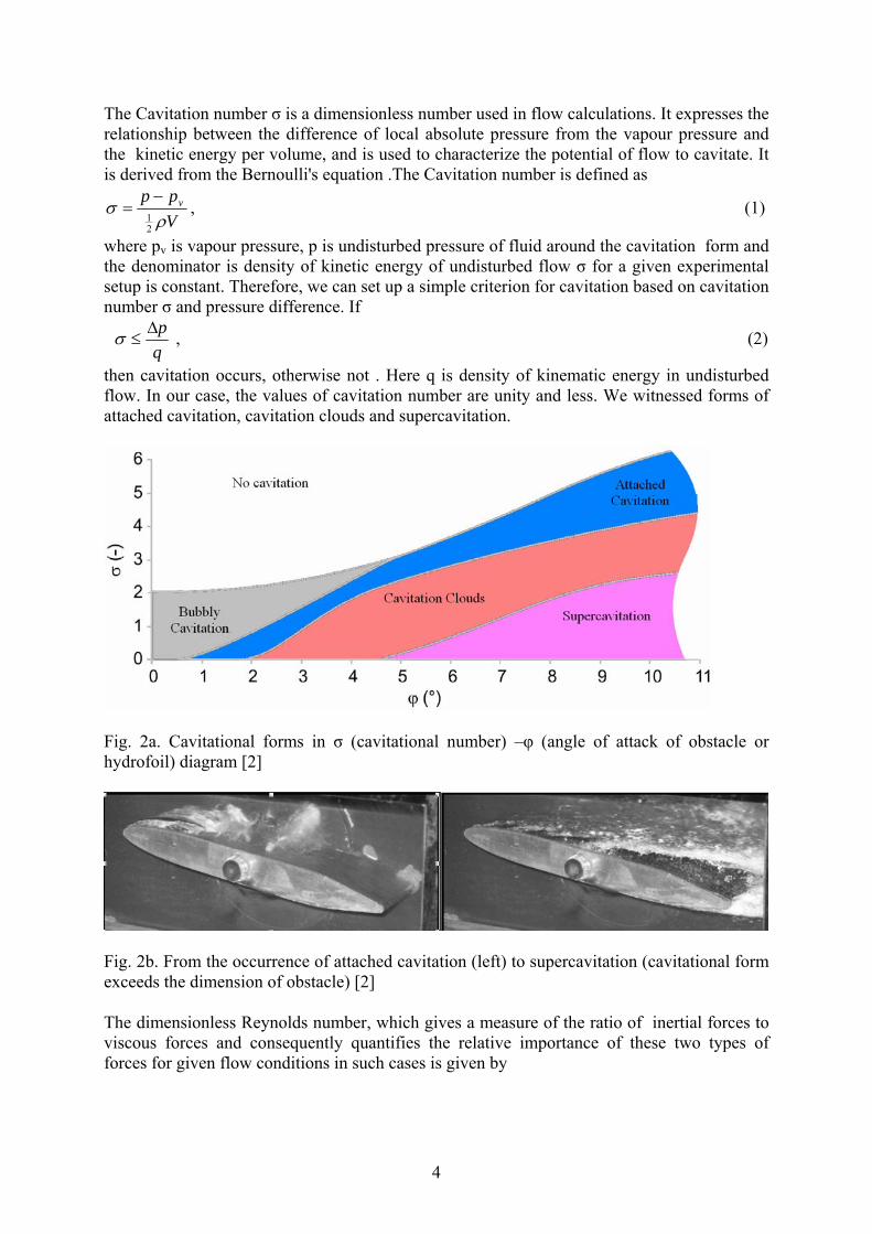
then cavitation occurs, otherwise not . Here q is density of kinematic energy in undisturbed flow. In our case, the values of cavitation number are unity and less. We witnessed forms of attached cavitation, cavitation clouds and supercavitation.

Fig. 2a. Cavitational forms in σ (cavitational number) –φ (angle of attack of obstacle or hydrofoil) diagram [2]

Fig. 2b. From the occurrence of attached cavitation (left) to supercavitation (cavitational form exceeds the dimension of obstacle) [2]

The dimensionless Reynolds number, which gives a measure of the ratio of inertial forces to viscous forces and consequently quantifies the relative importance of these two types of forces for given flow conditions in such cases is given by

5

νμ

ρ vLvL==Re , (3)

Where v is speed of laminar flow of the fluid, L is characteristic length of flow (for evaluation we take dimension of the test section in our case 10 cm) and ν is kinematic viscosity .In case of our experiment the value of Re is in order of 105 (for rapid flow around geometric obstacle, order of velocity 10 m/s and at room temperature). For such order of Re number turbulent flow is normally quite unstable,. The occurrence of cavitation is called cavitation inception. Pure fluid, in our case water, can withstand considerable low pressure (i.e. negative tension) without undergoing tension. A necessary condition for inception is the presence of weak spots in the fluid, which break the bond between fluid molecules. In the beginning of Venturi profile we expect cavitation inception, which normally occurs with standard cavitation numbers.

1.3. Known velocimetry methods in two phase flows Note that theoretical background for this seminar is presently still weak. The theoretical knowledge is mostly related to spherical cavitation clouds. In such a cloud we can assume the existence of smaller spherical bubbles with some distribution [4] . If spherical cloud travels to an area of sufficiently low pressure, it will cavitate, in other words the bubbles will grow explosively too many times from their original size. Subsequently, if the pressure far from the cloud increases again, the bubbles will collapse violently. For single bubble the theoretical background is given by Rayleigh- Plesset equation to model the highly non-linear reaction of the single bubble[3]

RdtdR

RdtdR

dtRdRtptp

L

L

L

B

ργν

ρ24

23)()( 2

2

2

++⎟⎠⎞

⎜⎝⎛+=

− ∞ (4)

This is an approximate equation derived from the incompressible Navier Stokes equations, written in the spherical coordinate system. It describes the motion of bubble radius R as a function of time t. The equation includes the phenomena of dynamics, viscosity, pressure and surface tension. For a cloud of bubbles this is more complex and requires the use of continuity and momentum equations coupled to the Rayleigh- Plesset equation in order to model the two-phase flow within the cloud. Velocity measurements within cavitating flows encounter strong difficulties. Only a few results have been obtained so far, although such experiments may be a key for physical modelling of cavitation. Some techniques so far include PIV (particle image velocimetry) in the USA (J. Katz team 2000 and Arndt group 2005) in the wake of sheet cavities, LIF (Laser induced fluorescence) in Germany (Dular, 2004 in 2007) and double optical probe measurements performed in the LEGI laboratory in France by Stutz and Reboued (1997). The main limitation of these approaches is that they only provide the flow velocity of one phase. Also, no dynamic information is accessible. The technique with optical sensors is integrated simultaneously, and PIV was realized at a few Hz. For these reasons, a technique based on X-ray absorption was proposed as well as phase contrast enhancement. This technique allows to carry out measurements at kHz time frequency. The measurement uncertainties are evaluated to be in the magnitude of percents, same as PIV. 2. ULTRA FAST X-RAY IMAGING AND EXPERIMENTAL SETUP

6

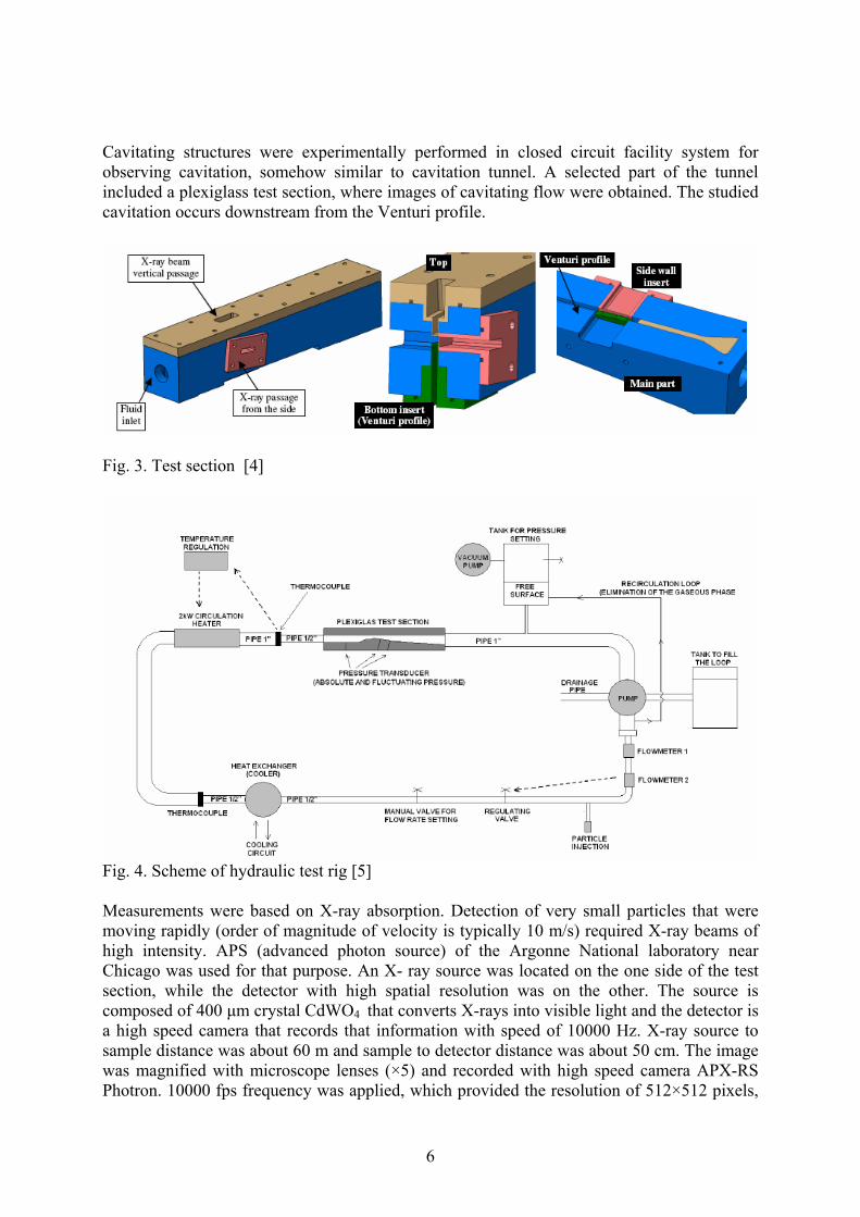
Cavitating structures were experimentally performed in closed circuit facility system for observing cavitation, somehow similar to cavitation tunnel. A selected part of the tunnel included a plexiglass test section, where images of cavitating flow were obtained. The studied cavitation occurs downstream from the Venturi profile.

Fig. 3. Test section [4]

Fig. 4. Scheme of hydraulic test rig [5] Measurements were based on X-ray absorption. Detection of very small particles that were moving rapidly (order of magnitude of velocity is typically 10 m/s) required X-ray beams of high intensity. APS (advanced photon source) of the Argonne National laboratory near Chicago was used for that purpose. An X- ray source was located on the one side of the test section, while the detector with high spatial resolution was on the other. The source is composed of 400 μm crystal CdWO4 that converts X-rays into visible light and the detector is a high speed camera that records that information with speed of 10000 Hz. X-ray source to sample distance was about 60 m and sample to detector distance was about 50 cm. The image was magnified with microscope lenses (×5) and recorded with high speed camera APX-RS Photron. 10000 fps frequency was applied, which provided the resolution of 512×512 pixels,

7

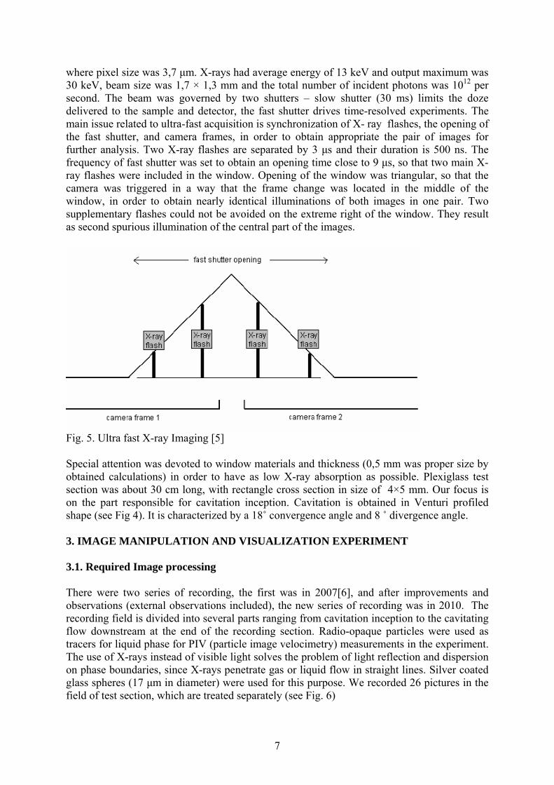
where pixel size was 3,7 μm. X-rays had average energy of 13 keV and output maximum was 30 keV, beam size was 1,7 × 1,3 mm and the total number of incident photons was 1012 per second. The beam was governed by two shutters – slow shutter (30 ms) limits the doze delivered to the sample and detector, the fast shutter drives time-resolved experiments. The main issue related to ultra-fast acquisition is synchronization of X- ray flashes, the opening of the fast shutter, and camera frames, in order to obtain appropriate the pair of images for further analysis. Two X-ray flashes are separated by 3 μs and their duration is 500 ns. The frequency of fast shutter was set to obtain an opening time close to 9 μs, so that two main X-ray flashes were included in the window. Opening of the window was triangular, so that the camera was triggered in a way that the frame change was located in the middle of the window, in order to obtain nearly identical illuminations of both images in one pair. Two supplementary flashes could not be avoided on the extreme right of the window. They result as second spurious illumination of the central part of the images.

Fig. 5. Ultra fast X-ray Imaging [5] Special attention was devoted to window materials and thickness (0,5 mm was proper size by obtained calculations) in order to have as low X-ray absorption as possible. Plexiglass test section was about 30 cm long, with rectangle cross section in size of 4×5 mm. Our focus is on the part responsible for cavitation inception. Cavitation is obtained in Venturi profiled shape (see Fig 4). It is characterized by a 18˚ convergence angle and 8 ˚ divergence angle. 3. IMAGE MANIPULATION AND VISUALIZATION EXPERIMENT 3.1. Required Image processing There were two series of recording, the first was in 2007[6], and after improvements and observations (external observations included), the new series of recording was in 2010. The recording field is divided into several parts ranging from cavitation inception to the cavitating flow downstream at the end of the recording section. Radio-opaque particles were used as tracers for liquid phase for PIV (particle image velocimetry) measurements in the experiment. The use of X-rays instead of visible light solves the problem of light reflection and dispersion on phase boundaries, since X-rays penetrate gas or liquid flow in straight lines. Silver coated glass spheres (17 μm in diameter) were used for this purpose. We recorded 26 pictures in the field of test section, which are treated separately (see Fig. 6)

8

Fig. 6. Recording field of test section in 2010 [5] Each position provides a number of image pairs made by X-ray imaging, recorded in selected time. X-rayed images first have to be prepared for the velocimetry experiment. Our first goal was to separate the desired area of flow from the background and to gain as uniform brightness of the pictures as possible for further treatment. A grey level image, made by the high speed camera, looks like this

Fig. 7. Raw recorded image (2007) Rotation for better orientation and image cropping are simple tasks which can be made with the selected software. Note that the part above the cavitation flow in the image is treated as unimportant and will be cropped. Achieving uniform brightness turned out to be a difficult task due to technical problems and required analysis of image brightness both in vertical and horizontal dimension since known software filtering algorithms did not fulfill our needs. With subprogram in LabView, called Horizontal analysis, we first measured approximate brightness of grey levels (containing discrete values from 0 to 256 in our case) in all points of straight lines for selected heights of image and then divided them by the number of heights. In doing so we obtained the average profile of grey level values according to x-coordinate of picture. Then we set new values of grey levels, compared with the average value of brightness in the entire image. In the selected x – coordinate we entered the values in y-direction and corrected them with the additional value of the difference between average grey level of the entire image and average grey level value of the straight line on the x-coordinate. The attempt at formulation is as follows:

⎥⎥⎦

⎤

⎢⎢⎣

⎡−⎟⎟

⎠

⎞⎜⎜⎝

⎛+= ∑∑ ∑

== =

),()),((),(),(1

1

1 1

11'jp

n

pn

m

k

n

pkpnmjiji yxIyxIyxIyxI (5)

9

Analogously this was made for vertical operation, only the directions were changed. The subprogram used is called Vertical equalization. We noticed two problems in the images – belts of brighter grey levels in the middle and low grey levels on the horizontal edges. The whole programme, combining both subprogrammes, provided respectful results for further work. Examples are shown in images below. Note that the correction of pictures could be made with several other operations (for example multiplying with proper weights) in both programmes, Vertical equalization vi and Horizontal equalization vi.

Fig. 8. Random pair of investigated pictures (2007) before equalization (left) and after equalization (right).

Fig 9 Distribution of grey level intensity before the use of Horizontal and Vertical equalization (left chart) and after (right chart) on a random image Fear of losing some information in the following steps of our research was present, but calculations yield satisfying results. In the next step we tried to eliminate opaque particles and separate vapour phase from liquid phase where possible. A large area of the observed test section can be marked as a separate multiphase flow and is ideal for our investigation. Both phases are distinguished by visual edge in the images. The inner part of the bubbles or bubble clouds is brighter than the main , since X-ray absorption is lower in vapour than in liquid. In that case we combined some morphological operations in LabView to detect the edge that separates both phases. For detecting vapour, high values of threshold were applied in order to identify pixels with high value of grey level. In addiction, conditions on shape, size and concentration are also applied: this last condition aims at detecting only vapour areas, instead of regions characterized by high concentrations of small objects that may be particles. Most important is the following condition: it is imposed that vapour areas should be in contact with one interface at previous step. Particle filtering is also an important task in vapour phase. For treatment of vapour phase, spatial filtering is applied to eliminate particles in the images. A linear filter is used by

10

convoluting a kernel matrix over the entire image. In the vicinity where cavitation occurs and in the area of cloud cavitation, where cavitation clouds are nicely confined between solid obstacle and fluid, such separations provide favourable results. At the end of cavitating structures downstream the test section, where cavitating clouds are in many cases torn apart into so called travelling cavitation bubbles, which often collapse in the area of higher pressure, we are faced with a problem of disperse flow. Some isolated bubbles are often treated as part of a fluid phase. But calculations show that visual separation is in more than 90 % cases successful.

Fig. 10. Control panels in LabView’s morphological operations and final phase separation: vapour phase is coloured grey and liquid phase is coloured dark (right windows) 3.2. Mathematical operations for translation We operate with pairs of images, delayed for estimated time by two consecutive X-ray flashes. First picture is divided into an array of equidistant points, where displacements are observed. The distance between two neighbouring points in the array is Δ. A square template is constructed around each point. Template size is experimentally determined. Every kind of that image pattern of selected size from the first image is then searched for in the next image of the selected pair. Furthermore, this is not just a search for displacements of the squares patterns, since the process also involves the rotation of square pattern with software tools. The similarity of two patterns is tested with cross-correlation method, already used in PIV technique . For better understanding a brief introduction of PIV technique is provided as well as its comparison to our experimental programme in vapour phase. 3.2.1 Basics of PIV Technique PIV is a visualization measurement method able to partially determine the instantaneous velocity gradient tensor ∂u/∂x within the plane defined by the light sheet. This implies that PIV measurement can be used to determine the instantaneous out-of-plane component of vorticity, i. e., the curl of the velocity field. An additional contribution of PIV technique to experimental research is its capability to simultaneously determine flow velocity at a large number of points, which allows a significant reduction of the time required to obtain experimental data. The extension of the PIV technique into a three dimensional measurement method has been achieved by different approaches:

11

• high-speed scanning method (the quasi-instantaneous three-dimensional flow structure is reconstructed from PIV recordings obtained at high repetition rate over parallel planes slightly shifted along the normal direction

• holographic recording • three-dimensional scattered light field reconstruction algorithm based on digital

tomography

In PIV the motion of a fluid is visualized by the motion of small tracer particles added to the fluid. These tracer particles constitute a pattern that can be used to evaluate the fluid motion. If tracer density is very low (i. e., the distance between distinct particles is much larger than the displacement) then it is relatively easy to evaluate the displacement of individual tracer particles. This mode of operation is generally referred to as low-image-density PIV, or particle tracking velocimetry (PTV). By increasing the concentration of tracer particles, the displacement becomes larger than the particle-image spacing, and it is no longer possible to identify matching pairs unambiguously. This mode of operation is generally referred to as high-image-density PIV. 3.2.2 Digital image correlation (DIC) DIC is predicated on the maximization of a correlation coefficient which is determined by examining pixel intensity array subsets in two or more corresponding images and extracting the deformation mapping function that relates to the images. An iterative approach is used to minimize the 2D correlation coefficient by applying non-linear optimization techniques. The cross correlation coefficient rij is defined as [7]

[ ]∑ ∑

∑−−

−−−=

∂∂

∂∂

∂∂

∂∂

ji jijiji

jijiji

ijGyxGFyxF

GyxGFyxF

yv

xv

yu

xuvur

, ,

2**2

,

**

)),(()),((

)),()(),((1),,,,,( (6)

Here F(xi ,yj) is pixel intensity or the grey scale value at point (xi ,yj) in the undeformed image. G(xi

* ,yj*) is gray scale value at point (xi

* ,yj*) in the deformed image. and are

mean values of the intensity matrices F and G, respectively. The coordinates or grid points (xi ,yj) and (xi

* ,yj*) are related by the deformation that occurs between the two images. If the

motion is perpendicular to the optical axis of the camera, then the relation between (xi ,yj) and (xi

* ,yj*) can be approximated by a 2D affine transformation such as:

yyvx

xvvyy

yyux

xuuxx

Δ∂∂

+Δ∂∂

++=

Δ∂∂

+Δ∂∂

++=

∗

*

(7)

Here u and v are translations of the centre of the sub-image in X and Y direction, respectively. The distances from the centre of sub-image to point (x, y) are denoted by Δx and Δy. Thus, the correlation coefficient rij is a function of displacement components (u, v) and displacement gradients. Spatial methods operate in the image domain, matching intensity patterns or features in images. Frequency-domain methods find the transformation parameters for registration of images while working in the transform domain. Such methods work for simple transformations, i.e. translation, rotation and scaling. Applying the phase correlation

12

method to a pair of images produces a third image which contains a single peak. The location of this peak corresponds to the relative translation between the images. Unlike many spatial-domain algorithms, the phase correlation method is resilient to noise, occlusions and other defects typical of medical or satellite images. Additionally, the phase correlation uses the fast Fourier transform (FFT) to compute the cross-correlation between two images, generally resulting in large performance gains. Image I (x, y) is discretized by the image sensor (i. e. camera device) that integrates the light intensity over a small area, or pixel: [ ] ∫∫ ⋅−⋅−= dxdyyxIdjydixpjiI ),(),(, ττ (8)

where p(x, y) is pixel spatial sensitivity. This is usually a uniform rectangular area, but more complex forms should be used to represent the effect of microlenses (where the sensitivity may be non-uniform and leakage from adjacent pixels can be incorporated). Image intensity is represented in a finite number of discrete levels. Common quantization level ranges are 256 or 4096 gray levels, i. e., 8 bit and 12 bit quantization, respectively. The quantization can be represented as additive white noise [ ] [ ] [ ]jijiIjiI ,,, ζ+= • (9)

When the variance of ζ is small with respect to the variance of I , the effect of quantization can be ignored. Usually the sensor noise level is larger than the quantization noise level. Therefore I • is simply written as I . Extreme situation is a binary image (which contains only gray levels 0 and 1), which is sometimes used to implement a special form of spatial correlation; in that case the increased noise contribution of ζ needs to be compensated by a higher image density. For digital images I1[i,j] and I2[i,j] the discrete spatial correlation is given by

[ ] [ ] [ ] [ ] ),(,),(, 222,

111 IkjpiIkjpiWIjiIjiWrji

pk −++++⋅−=∑ (10)

where I 1 and I 2 are the averaged image values over windows W1 and W2, respectively. Commonly, W1 and W2 are identical and uniform N × N pixel domains, equal to 1 inside the domain and zero outside the domain. For faster evaluation of spatial correlation, FFT is used. One of the most powerful aspects of digital PIV is its ability to determine the particle-image displacement at subpixel level: under optimal conditions the particle-image displacement can be estimated with a precision better than 0.1 pixel. The peak location at subpixel level is obtained by interpolation of the correlation values around the correlation maximum.

Fig. 11 The correlation values in a narrow peak as a function of subpixel position of displacement-correlation peak (one dimension). Fig. 11 shows a concrete example of primitive peak detection. Note that value φ0 ≡ φ[m0, n0] of the correlation maximum remains practically unchanged, while the two adjacent correlation values φ−1 ≡ φ[m0 −1, n0] and φ+1 ≡ φ[m0+1, n0] change considerably in amplitude. This means that subpixel location of maximum (i. e. the particle-image displacement) can be estimated based on correlation values {φ−1, φ0, φ+1} for each coordinate. The most commonly used method for sub-pixel estimation of displacement is the three-point Gaussian peak fit, where the subpixel part for each component of the displacement is given by

13

)ln2ln(ln2)ln(ln

011

11

rrrrr

X −−−

=+−

+−ε (11)

If image background is non-uniform, i.e. there are no light reflections (as it was in our case after some image processing), this is true estimation. Otherwise there are some other methods proposed to detect position of correlation peak. [8] In vapour phase visual complexity bubble clouds contain enough information to recognize small patterns, so tracers are not required anymore. Anyway, the software still uses the same principles as in PIV, i.e. image pattern recognition through cross correlation combined with the possible rotation of selected pattern. 3.3 Correction of the first velocimetry results and some improvements Pattern matching in the software is shown as an array with few information: quality of matching (from 1000 (perfect) to 0 (none)) and coordinates of centre of new matching pattern in the second picture and its rotation. Pattern matching is ordered by the quality of patterns starting with the best result to the threshold of least but still acceptable results. We set the lowest threshold to experimentally determined level. We have to reject random errors in pattern matching and repair them by assuming that velocity field should follow continuity. There are two approaches – to reject all results with discontinuity in the velocity field and accept the next best result if it fits the condition, or replace them with interpolation in neighbouring points. The next step is to test the results by the variability of pattern size. We determine dimension of patterns around the same point and search for a match in next image. Then we examine the results with statistical tools. We mark the area of reliable measurements. The velocity vectors close to the edge of images are often inappropriate due to lack of information. On the edge of each image we only consider the results, which fully fit into the next image. If we gain some discontinuity on the edges, we test the result with statistical tools in the vicinity of the neighbouring points. In the final phase we draw the vectors with arrows in the first image to show the velocity filed with the help of software. 4. RESULTS AND OBSERVATIONS There were a few series of X ray recordings in 2007, most of them vary due to flow rate (from 10 l/min to 16 l/min). The behaviour at different flow conditions was observed and compared. The behaviour of different cavitational forms and their parts was observed as well. Nevertheless that cavitation flow was fully turbulent at this Re numbers, it had some pattern of evolution from cavitation inception to travelling bubble cavitation (where cavitation cloud collapses into many smaller units). This is the matter of current research.

14

0

50

100

150

200

250

300

350

400

0 10 20 30 40 50 60

index of point on selected positon of recording

RRE

Fig. 12. Better success in pattern matching (without corrections) before the process of image equalization (R) and after (RE) in 2007 recordings. Fig. 12 demonstrates the improvement in software processing before and after image preparation. In retrospect our selected recording position was divided into 50 points, we kept the optimal window size (40 pixels) and recorded the first 1000 pairs of images. Then a test was performed with software pattern matching by calculating the velocities. The number of failed pattern matchings (y-axis) was observed in selected points for one recording position (x-axis) in both cases. The biggest problems occurred at the edge of the images (peaks). That is why the area of investigation was reduced as mentioned.

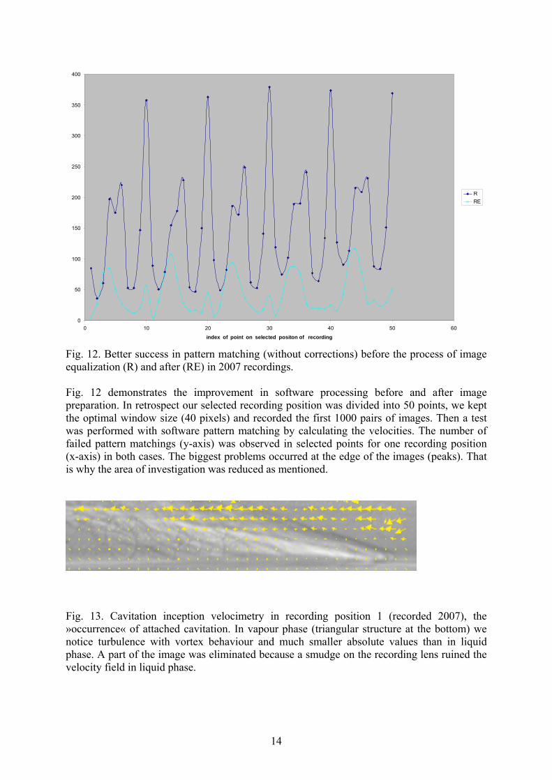
Fig. 13. Cavitation inception velocimetry in recording position 1 (recorded 2007), the »occurrence« of attached cavitation. In vapour phase (triangular structure at the bottom) we notice turbulence with vortex behaviour and much smaller absolute values than in liquid phase. A part of the image was eliminated because a smudge on the recording lens ruined the velocity field in liquid phase.

15

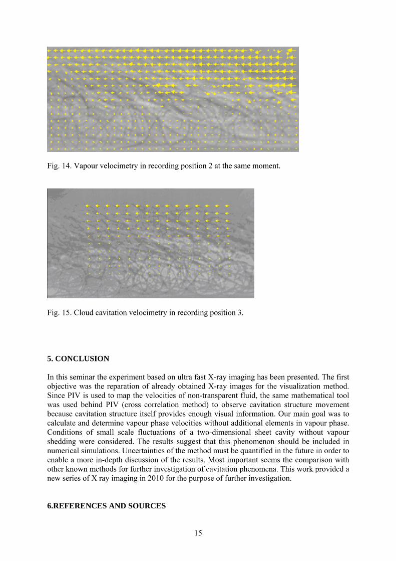
Fig. 14. Vapour velocimetry in recording position 2 at the same moment.

Fig. 15. Cloud cavitation velocimetry in recording position 3. 5. CONCLUSION In this seminar the experiment based on ultra fast X-ray imaging has been presented. The first objective was the reparation of already obtained X-ray images for the visualization method. Since PIV is used to map the velocities of non-transparent fluid, the same mathematical tool was used behind PIV (cross correlation method) to observe cavitation structure movement because cavitation structure itself provides enough visual information. Our main goal was to calculate and determine vapour phase velocities without additional elements in vapour phase. Conditions of small scale fluctuations of a two-dimensional sheet cavity without vapour shedding were considered. The results suggest that this phenomenon should be included in numerical simulations. Uncertainties of the method must be quantified in the future in order to enable a more in-depth discussion of the results. Most important seems the comparison with other known methods for further investigation of cavitation phenomena. This work provided a new series of X ray imaging in 2010 for the purpose of further investigation. 6.REFERENCES AND SOURCES

16

[1] http://www.gidb.itu.edu.tr/staff/emin/Lectures/Ship_Hydro/cavitation.pdf [2]KAVITACIJA, B. Širok, M. Dular,B. Stoffel, Ljubljana 2006 [3] http://authors.library.caltech.edu/25017/1/cavbubdynam.pdf, CAVITATION AND BUBBLY DYNAMICS, C.E. Brennen, Oxford University Press 1995 [4] CLOUD CAVITATION PHENOMENA http://authors.library.caltech.edu/53/

[5] VELOCITY MEASUREMENTS IN CAVITATING FLOWS BY FAST X-RAY IMAGING, Olivier Coutier-Delgosha, Marko Hocevar, Ilyass Khlifa, Sylvie Fuzier, Alexandre Vabre, Kamel Fezzaa, Wah-Keat Lee, 14th international Symposium on Transport Phenomena and Dynamics of Rotating Machinery , Honolulu 2012

[6]http://www.sciencedirect.com/science/article/pii/S0168900209006470

[7] http://en.wikipedia.org/wiki/Digital_image_correlation

[8] SPRINGER HANDBOOK OF EXPERIMENTAL FLUID MECHANICS, Cameron Tropea, Alexander L. Yarin, John F. Foss, Springer 2007

1.BUBBLY CLOUD DYNAMICS AND CAVITATION, C. E: Brennen, CIT , Pasadena California, Invited lecture at the Acoustical Society of America Meeting, June 2007, Salt lake City, Utah