OCT methods for capillary velocimetry

OCT methods for capillary velocimetry Vivek J. Srinivasan,1,* Harsha Radhakrishnan,2 Eng H. Lo,3 Emiri T. Mandeville,3

James Y. Jiang,4 Scott Barry,4 and Alex E. Cable4 1MGH/MIT/HMS Athinoula A. Martinos Center for Biomedical Imaging, Department of Radiology,

Massachusetts General Hospital/Harvard Medical School, Charlestown, MA 02129, USA 2Center for Neural Engineering, Pennsylvania State University, University Park, PA 16802, USA

3Neuroprotection Research Laboratory, Departments of Radiology and Neurology, Massachusetts General Hospital/Harvard Medical School, Charlestown, MA 02129, USA

4Advanced Imaging Group, Thorlabs, Inc., Newton, NJ 07860, USA *[email protected]

Abstract: To date, two main categories of OCT techniques have been described for imaging hemodynamics: Doppler OCT and OCT angiography. Doppler OCT can measure axial velocity profiles and flow in arteries and veins, while OCT angiography can determine vascular morphology, tone, and presence or absence of red blood cell (RBC) perfusion. However, neither method can quantify RBC velocity in capillaries, where RBC flow is typically transverse to the probe beam and single-file. Here, we describe new methods that potentially address these limitations. Firstly, we describe a complex-valued OCT signal in terms of a static scattering component, dynamic scattering component, and noise. Secondly, we propose that the time scale of random fluctuations in the dynamic scattering component are related to red blood cell velocity. Analysis was performed along the slow axis of repeated B-scans to parallelize measurements. We correlate our purported velocity measurements against two-photon microscopy measurements of RBC velocity, and investigate changes during hypercapnia. Finally, we image the ischemic stroke penumbra during distal middle cerebral artery occlusion (dMCAO), where OCT velocimetry methods provide additional insight that is not afforded by either Doppler OCT or OCT angiography. © 2012 Optical Society of America OCIS codes: (110.4500) Optical coherence tomography; (170.3880) Medical and biological imaging; (170.5380) Physiology; (170.1470) Blood or tissue constituent monitoring; (170.0180) Microscopy; (170.6900) Three-dimensional microscopy.

References and links 1. A. Grinvald, E. Lieke, R. D. Frostig, C. D. Gilbert, and T. N. Wiesel, “Functional architecture of cortex revealed

by optical imaging of intrinsic signals,” Nature 324(6095), 361–364 (1986). 2. A. Villringer and B. Chance, “Non-invasive optical spectroscopy and imaging of human brain function,” Trends

Neurosci. 20(10), 435–442 (1997). 3. B. A. Wilt, L. D. Burns, E. T. Wei Ho, K. K. Ghosh, E. A. Mukamel, and M. J. Schnitzer, “Advances in light

microscopy for neuroscience,” Annu. Rev. Neurosci. 32(1), 435–506 (2009). 4. U. Dirnagl, B. Kaplan, M. Jacewicz, and W. Pulsinelli, “Continuous measurement of cerebral cortical blood flow

by laser-Doppler flowmetry in a rat stroke model,” J. Cereb. Blood Flow Metab. 9(5), 589–596 (1989). 5. A. K. Dunn, H. Bolay, M. A. Moskowitz, and D. A. Boas, “Dynamic imaging of cerebral blood flow using laser

speckle,” J. Cereb. Blood Flow Metab. 21(3), 195–201 (2001). 6. E. M. Hillman, D. A. Boas, A. M. Dale, and A. K. Dunn, “Laminar optical tomography: demonstration of

millimeter-scale depth-resolved imaging in turbid media,” Opt. Lett. 29(14), 1650–1652 (2004). 7. W. Denk, J. H. Strickler, and W. W. Webb, “Two-photon laser scanning fluorescence microscopy,” Science

248(4951), 73–76 (1990). 8. Z. Chen, T. E. Milner, D. Dave, and J. S. Nelson, “Optical Doppler tomographic imaging of fluid flow velocity

in highly scattering media,” Opt. Lett. 22(1), 64–66 (1997). 9. J. A. Izatt, M. D. Kulkarni, S. Yazdanfar, J. K. Barton, and A. J. Welch, “In vivo bidirectional color Doppler flow

imaging of picoliter blood volumes using optical coherence tomography,” Opt. Lett. 22(18), 1439–1441 (1997).

#158450 - $15.00 USD Received 1 Dec 2011; revised 14 Feb 2012; accepted 17 Feb 2012; published 24 Feb 2012(C) 2012 OSA 1 March 2012 / Vol. 3, No. 3 / BIOMEDICAL OPTICS EXPRESS 612

10. R. Leitgeb, C. K. Hitzenberger, and A. F. Fercher, “Performance of Fourier domain vs. time domain optical coherence tomography,” Opt. Express 11(8), 889–894 (2003).

11. B. R. White, M. C. Pierce, N. Nassif, B. Cense, B. H. Park, G. J. Tearney, B. E. Bouma, T. C. Chen, and J. F. de Boer, “In vivo dynamic human retinal blood flow imaging using ultra-high-speed spectral domain optical coherence tomography,” Opt. Express 11(25), 3490–3497 (2003).

12. B. J. Vakoc, R. M. Lanning, J. A. Tyrrell, T. P. Padera, L. A. Bartlett, T. Stylianopoulos, L. L. Munn, G. J. Tearney, D. Fukumura, R. K. Jain, and B. E. Bouma, “Three-dimensional microscopy of the tumor microenvironment in vivo using optical frequency domain imaging,” Nat. Med. 15(10), 1219–1223 (2009).

13. D. Huang, E. A. Swanson, C. P. Lin, J. S. Schuman, W. G. Stinson, W. Chang, M. R. Hee, T. Flotte, K. Gregory, C. A. Puliafito, and et, “Optical coherence tomography,” Science 254(5035), 1178–1181 (1991).

14. Y. Wang, B. A. Bower, J. A. Izatt, O. Tan, and D. Huang, “In vivo total retinal blood flow measurement by Fourier domain Doppler optical coherence tomography,” J. Biomed. Opt. 12(4), 041215 (2007).

15. V. J. Srinivasan, S. Sakadzić, I. Gorczynska, S. Ruvinskaya, W. Wu, J. G. Fujimoto, and D. A. Boas, “Quantitative cerebral blood flow with optical coherence tomography,” Opt. Express 18(3), 2477–2494 (2010).

16. D. Kleinfeld, P. P. Mitra, F. Helmchen, and W. Denk, “Fluctuations and stimulus-induced changes in blood flow observed in individual capillaries in layers 2 through 4 of rat neocortex,” Proc. Natl. Acad. Sci. U.S.A. 95(26), 15741–15746 (1998).

17. S. Makita, Y. Hong, M. Yamanari, T. Yatagai, and Y. Yasuno, “Optical coherence angiography,” Opt. Express 14(17), 7821–7840 (2006).

18. R. K. Wang, S. L. Jacques, Z. Ma, S. Hurst, S. R. Hanson, and A. Gruber, “Three dimensional optical angiography,” Opt. Express 15(7), 4083–4097 (2007).

19. Y. K. Tao, A. M. Davis, and J. A. Izatt, “Single-pass volumetric bidirectional blood flow imaging spectral domain optical coherence tomography using a modified Hilbert transform,” Opt. Express 16(16), 12350–12361 (2008).

20. A. Mariampillai, B. A. Standish, E. H. Moriyama, M. Khurana, N. R. Munce, M. K. Leung, J. Jiang, A. Cable, B. C. Wilson, I. A. Vitkin, and V. X. Yang, “Speckle variance detection of microvasculature using swept-source optical coherence tomography,” Opt. Lett. 33(13), 1530–1532 (2008).

21. V. J. Srinivasan, J. Y. Jiang, M. A. Yaseen, H. Radhakrishnan, W. Wu, S. Barry, A. E. Cable, and D. A. Boas, “Rapid volumetric angiography of cortical microvasculature with optical coherence tomography,” Opt. Lett. 35(1), 43–45 (2010).

22. H. Ren, T. Sun, D. J. MacDonald, M. J. Cobb, and X. Li, “Real-time in vivo blood-flow imaging by moving-scatterer-sensitive spectral-domain optical Doppler tomography,” Opt. Lett. 31(7), 927–929 (2006).

23. A. Mariampillai, M. K. Leung, M. Jarvi, B. A. Standish, K. Lee, B. C. Wilson, A. Vitkin, and V. X. Yang, “Optimized speckle variance OCT imaging of microvasculature,” Opt. Lett. 35(8), 1257–1259 (2010).

24. J. Fingler, D. Schwartz, C. Yang, and S. E. Fraser, “Mobility and transverse flow visualization using phase variance contrast with spectral domain optical coherence tomography,” Opt. Express 15(20), 12636–12653 (2007).

25. H. Ren, K. M. Brecke, Z. Ding, Y. Zhao, J. S. Nelson, and Z. Chen, “Imaging and quantifying transverse flow velocity with the Doppler bandwidth in a phase-resolved functional optical coherence tomography,” Opt. Lett. 27(6), 409–411 (2002).

26. D. Piao, L. L. Otis, and Q. Zhu, “Doppler angle and flow velocity mapping by combined Doppler shift and Doppler bandwidth measurements in optical Doppler tomography,” Opt. Lett. 28(13), 1120–1122 (2003).

27. S. G. Proskurin, Y. He, and R. K. Wang, “Determination of flow velocity vector based on Doppler shift and spectrum broadening with optical coherence tomography,” Opt. Lett. 28(14), 1227–1229 (2003).

28. Y. Wang and R. Wang, “Autocorrelation optical coherence tomography for mapping transverse particle-flow velocity,” Opt. Lett. 35(21), 3538–3540 (2010).

29. P. J. Drew, A. Y. Shih, J. D. Driscoll, P. M. Knutsen, P. Blinder, D. Davalos, K. Akassoglou, P. S. Tsai, and D. Kleinfeld, “Chronic optical access through a polished and reinforced thinned skull,” Nat. Methods 7(12), 981–984 (2010).

30. S. Yousefi, Z. Zhi, and R. Wang, “Eigendecomposition-based clutter filtering technique for optical micro-angiography,” IEEE Trans. Biomed. Eng. 58(8), 2316–2323 (2011).

31. Y. Imai and K. Tanaka, “Direct velocity sensing of flow distribution based on low-coherence interferometry,” J. Opt. Soc. Am. A 16(8), 2007–2012 (1999).

32. H. L. Goldsmith and J. C. Marlow, “Flow behavior of erythrocytes. 2. Particle motions in concentrated suspensions of ghost cells,” J. Colloid Interface Sci. 71(2), 383–407 (1979).

33. Y. Park, M. Diez-Silva, D. Fu, G. Popescu, W. Choi, I. Barman, S. Suresh, and M. S. Feld, “Static and dynamic light scattering of healthy and malaria-parasite invaded red blood cells,” J. Biomed. Opt. 15(2), 020506 (2010).

34. J. Kalkman, R. Sprik, and T. G. van Leeuwen, “Path-length-resolved diffusive particle dynamics in spectral-domain optical coherence tomography,” Phys. Rev. Lett. 105(19), 198302 (2010).

35. E. B. Hutchinson, B. Stefanovic, A. P. Koretsky, and A. C. Silva, “Spatial flow-volume dissociation of the cerebral microcirculatory response to mild hypercapnia,” Neuroimage 32(2), 520–530 (2006).

36. M. Meinke, G. Müller, J. Helfmann, and M. Friebel, “Empirical model functions to calculate hematocrit-dependent optical properties of human blood,” Appl. Opt. 46(10), 1742–1753 (2007).

37. T. M. Fischer, M. Stöhr-Lissen, and H. Schmid-Schönbein, “The red cell as a fluid droplet: tank tread-like motion of the human erythrocyte membrane in shear flow,” Science 202(4370), 894–896 (1978).


38. H. H. Lipowsky, “Microvascular rheology and hemodynamics,” Microcirculation 12(1), 5–15 (2005). 39. T. Schmoll, C. Kolbitsch, and R. A. Leitgeb, “Ultra-high-speed volumetric tomography of human retinal blood

flow,” Opt. Express 17(5), 4166–4176 (2009). 40. R. Bonner and R. Nossal, “Model for laser Doppler measurements of blood flow in tissue,” Appl. Opt. 20(12),

2097–2107 (1981). 41. J. Fingler, R. J. Zawadzki, J. S. Werner, D. Schwartz, and S. E. Fraser, “Volumetric microvascular imaging of

human retina using optical coherence tomography with a novel motion contrast technique,” Opt. Express 17(24), 22190–22200 (2009).

1. Introduction

Optical imaging methods [1–3] have significantly impacted the field of neuroimaging and are now widely used to study cellular and vascular physiology in the brain. Currently, optical imaging modalities can be broadly classified into two groups: macroscopic methods using diffuse light (optical intrinsic signal imaging [1], laser Doppler imaging [4], laser speckle imaging [5], diffuse optical imaging [2], and laminar optical tomography [6]) which achieve spatial resolutions of hundreds of µm to millimeters, and microscopic methods (two-photon and confocal microscopy) which achieve micron-scale resolutions. Two-photon microscopy [7], in particular, is widely used in structural and functional imaging at the cellular and subcellular levels. While macroscopic imaging methods using diffuse light can achieve high penetration depths and large fields of view, they do not provide high spatial resolution. While microscopy achieves subcellular spatial resolution, the imaging speed, penetration depth, and field of view are limited.

Optical Coherence Tomography (OCT) possesses a unique combination of high imaging speed, penetration depth, field of view, and resolution and therefore occupies an important niche between the macroscopic and microscopic optical imaging technologies discussed above. Relative to the optical imaging technologies currently used for neuroscience research, OCT has several advantages. Firstly, OCT enables volumetric imaging with high spatiotemporal resolution in tens of seconds to a few minutes. By contrast, volumetric imaging with two-photon microscopy typically requires tens of minutes to a few hours. Secondly, OCT achieves high penetration depth. OCT rejects out-of-focus and multiple scattered light, enabling imaging at depths of greater than 1 mm in scattering tissue. By contrast, two-photon microscopy enables imaging depths of approximately 0.5 mm in scattering tissue. Third, OCT can be performed with long working distance, low numerical aperture (NA) objectives. Because the OCT depth resolution depends on the coherence length of light and not the confocal parameter (depth of field), low NA lenses may be used. This contrasts with two-photon microscopy, where high depth resolution and penetration depth in scattering tissue in vivo can be achieved only with high-NA water immersion objectives. The use of relatively low NA objectives allows OCT imaging of large fields of view, enabling the synthesis of microscopic and macroscopic information. Fourth, since OCT can measure well-defined volumes using predominantly single scattered light, quantitative assessment of hemodynamic parameters such as blood vessel diameter and blood flow using Doppler algorithms are possible [8–12]. Fifth, OCT is performed using intrinsic contrast alone, and does not require the use of dyes or extrinsic contrast agents. This capability is attractive for longitudinal studies where cumulative dye toxicity is a concern.

The first OCT systems were designed to image backscattered light intensity [13]. Doppler OCT (Fig. 1(a)) has shown promise for the non-invasive measurement of absolute blood flow in various organs in situ, including the retina [14] and brain [15]. In contrast with diffuse optical imaging techniques such as laser Doppler and laser speckle imaging, DOCT enables measurement of velocity axial projections in well-defined microscopic volumes [9], enabling unambiguous, quantitative measurements. However, DOCT measurements of absolute blood flow must satisfy two conditions in order to be quantitatively accurate. Firstly, the vessel of interest must have a well-defined transverse velocity profile. Secondly, the vessel of interest must not be perpendicular to the probe beam, so that flow results in a measurable Doppler


f

B

Hhpf(f)

OCT AngiographyPower Spectral Density P(f)

f

Capillary VelocimetryPower Spectral Density P(f)

C

Δf~v

Dynamic scattering

Static scattering

f

A Doppler OCTPower Spectral Density P(f)

f0~vz

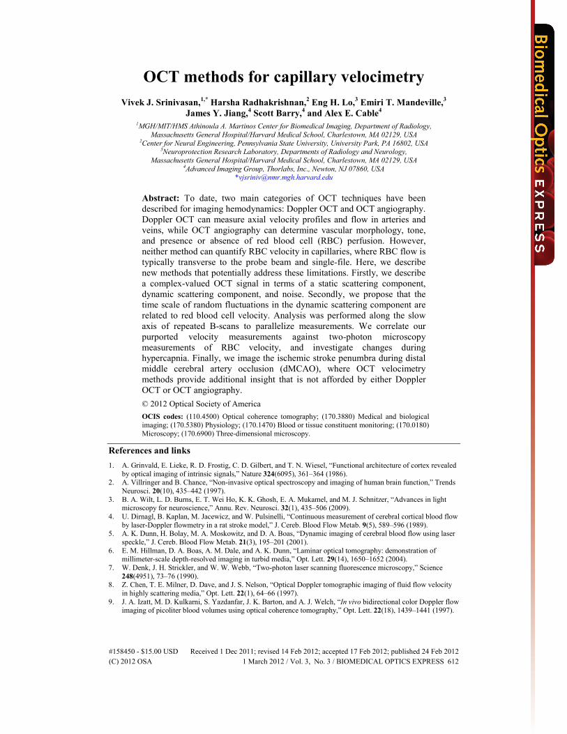
Fig. 1. Frequency domain comparison of Doppler OCT (a), OCT angiography (b), and the proposed method of OCT velocimetry (c). (a) In Doppler OCT, the center frequency of the dynamic scattering component of the power spectral density is estimated, and used to determine the axial projection of velocity, vz. (b) In conventional OCT angiography, a high-pass filter is applied to suppress static scattering, and visualize only the dynamic scattering component. (c) In the method of OCT velocimetry presented here, the spectral width of the dynamic scattering component is estimated.

shift. For instance, Doppler OCT is well-suited for measuring flow in ascending venules of >20 micron size in the cortex [15], where both of these conditions are met. However, conventional DOCT cannot measure dynamics in capillaries where, flow may be predominantly transverse to the probe beam by virtue of the imaging geometry, red blood cell (RBC) velocity is frequently between 0 and 1 mm / s, and RBC flow is single file [16]. A quantitative OCT metric of capillary perfusion would complement Doppler OCT measurements of flow, and would represent an important advance for in vivo hemodynamic imaging.

Recently, OCT angiography techniques that visualize vasculature in vivo [12,17–21] have emerged. An important insight, crucial to the development of OCT angiography techniques, was the recognition that the power spectral density within a single voxel can be represented as a superposition of static and dynamic scattering [19,22]. OCT angiography techniques seek to suppress static scattering from tissue in order to visualize only the dynamic scattering component. Most published techniques for OCT angiography involve some form of high-pass filtering. Some techniques use the field magnitude [20,23], others techniques use the phase [12,24], while other techniques use the complex field [18,19,21], thus incorporating both magnitude and phase information. OCT angiography relies on the fact that dynamic scattering components in vasculature experience decorrelation and Doppler shifting, thereby generating components at high spectral frequencies. By applying a high-pass filter, static (low frequency) scattering components are suppressed while dynamic (high frequency) scattering components are preserved. The brightness of the OCT angiogram at a given voxel is essentially the integrated spectral power of that voxel within the high-pass filter pass band, as shown in Fig. 1(b). Therefore, the brightness of the OCT angiogram is determined both by the magnitude of the dynamic scattering component and the fraction of the power spectral density of the dynamic scattering component that falls within the pass band of the high pass filter. Hence, while OCT angiography visualizes regions that decorrelate over time, it does not provide information about the decorrelation rate. Stated another way, while OCT angiography visualizes regions that contain dynamic scattering, it does not provide information about the bandwidth. Therefore, while OCT angiography is useful for visualizing perfused vasculature, it does not provide quantitative information on velocity, which is an important parameter for the study of hemodynamics.

Here, we propose a new method for the quantitative study of capillary hemodynamics. The method is based on estimating the width (Δf = 1/Δτ) of the power spectrum of electric field amplitude and phase fluctuations caused by RBCs traversing a voxel, as shown in Fig. 1(c). This method represents an advance since conventional OCT angiography does not


quantitatively measure either the decorrelation rate or the width of the power spectrum Previous work has used power spectrum broadening to estimate transverse flow velocity [25]. The transverse velocity can be combined with axial velocity obtained from the Doppler shift to compute the total flow velocity as well as the Doppler angle [26], however, broadening of the power spectrum due to axial motion must also be taken into account in this calculation [27]. In a recent study the slope of the normalized intensity autocorrelation function was found to be proportional to the transverse velocity of an intralipid flow phantom [28]. Our method builds upon this previous work by 1) directly accounting for the effects of static scattering in the analysis and 2) parallelizing measurements by performing analysis along the slow axis of repeated B-scans.

In this work, we review the effects of static and dynamic scattering in a single voxel and propose a straightforward procedure to estimate Δf. We present simple models that motivate the investigation of Δf as an indicator of velocity. We create maps of Δf, which clearly show heterogeneous values in different capillaries branches, but consistent values along non-branching capillary segments. These data suggest that Δf maps provide information about capillary RBC dynamics that cannot be obtained from conventional angiograms. We correlate values of Δf obtained from OCT imaging with RBC velocity values obtained from two-photon microscopy line scans. We also provide examples of scenarios where Δf maps provide additional insight to complement Doppler OCT and OCT angiography. Taken together, these data show that our method of capillary velocimetry provides novel information to complement conventional OCT hemodynamic imaging.

2. Experimental methods

2.1. System description

A 1310 nm spectral/Fourier domain OCT microscope was used for in vivo imaging of the rat cortex [21]. The light source consisted of two superluminescent diodes combined with a 50/50 fiber coupler to yield a spectral bandwidth of 170 nm. The axial (depth) resolution was 3.6 μm in tissue, full-width-at-half-maximum, the transverse resolution was 3.6 μm (full-width-at-half-maximum), and the imaging speed was 47,000 axial scans per second (17.3 microsecond exposure time), achieved by an InGaAs line scan camera (Goodrich-Sensors Unlimited, Inc.). The camera sensitivity was set to “high” for imaging through a closed cranial window, and “medium” for imaging through a thinned skull cranial window. A 10x objective (3 cm working distance, Mitsutoyu) was used.

2.2. Animal preparation

Sprague–Dawley rats (250 g – 350 g) were prepared under isoflurane anesthesia (1.5–2.5% in 25% Oxygen, 75% air). After tracheotomy and femoral arterial and venous catheterization, the head was fixed in a stereotaxic frame, the scalp was retracted, and a ~5 mm × 5 mm area of skull over the somatosensory cortex was thinned to translucency. The IVth ventricle was opened to relieve intra-cerebral pressure, and the thinned skull area was removed along with the dura. 1.5% agarose (Fluka) in artificial cerebrospinal fluid [21] was placed onto the exposed cortex and covered with a small glass coverslip. The window was then sealed relative to the skull with dental acrylic to minimize brain motion. Following surgery, isoflurane was discontinued, and replaced with intravenous delivery of alpha-chloralose (30–40 mg/kg/h). Throughout data collection, the animals were mechanically ventilated with air and oxygen, and systemic blood pressure was monitored and maintained within the normal range (100 mm Hg ± 20 mm Hg). Unless otherwise stated, blood gas values were measured when necessary to ensure good systemic physiology (PaCO2 between 32 and 40 mmHg, PaO2 between 90 and 120 mmHg, and pH between 7.35 and 7.45). All animal procedures were reviewed and approved by the Subcommittee on Research Animal Care at Massachusetts General Hospital, where these experiments were performed.


For distal middle cerebral artery occlusion (dMCAO) experiments, a thinned-skull, glass coverslip-reinforced cranial window [29] over the cerebral cortex was created in a C57BL6/6 mouse from Charles River Lab, enabling imaging of the boundary between middle cerebral artery (MCA) and anterior cerebral artery (ACA) supplied territories. A burr hole (3 mm diameter) was drilled under saline cooling in the temporal bone overlying the distal MCA. The dura was kept intact. The exposed artery was occluded with microbipolar coagulation where it crosses the inferior cerebral vein. Rectal temperature was maintained at 37°C with a thermostat-controlled heating pad.

fτ

Δτ ~1/v

Δf~v

Id

Is

Autocorrelation |R(τ)| Power Spectral Density P(f)A B

Dynamic scattering

Static scattering

Dynamic scattering (Id)Static scattering (Is) Overlay

0.1 mm 0.1 mm 0.1 mm 0.1 mm

C D E FTotal scattering (I)

f0~vz

τ

Autocorrelation arg[R(τ)]

slope~vz

I

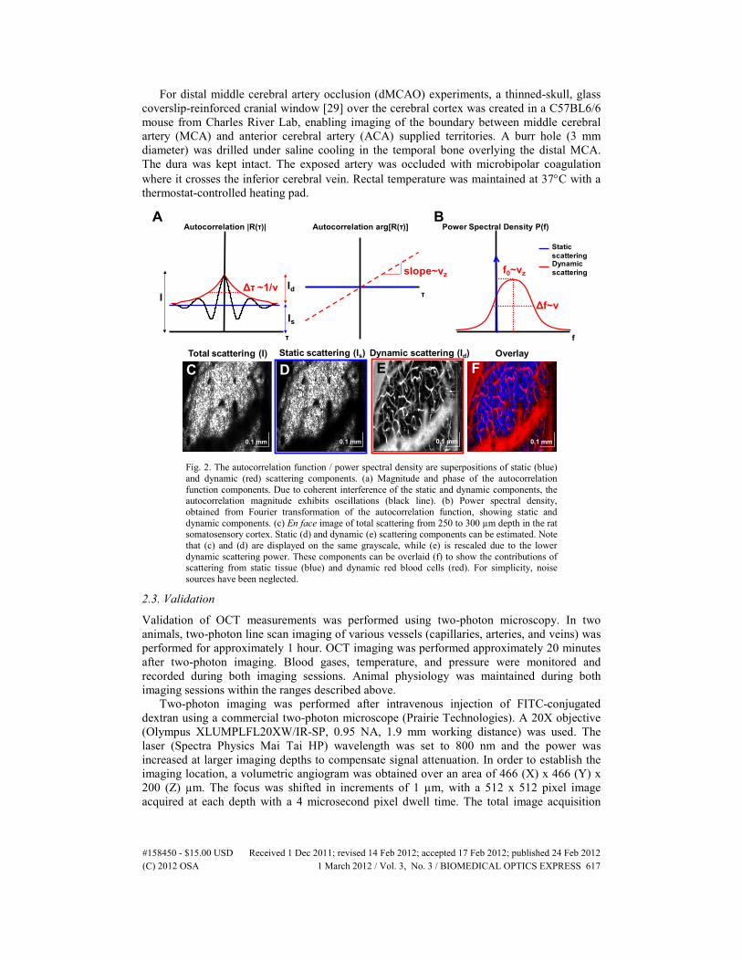
Fig. 2. The autocorrelation function / power spectral density are superpositions of static (blue) and dynamic (red) scattering components. (a) Magnitude and phase of the autocorrelation function components. Due to coherent interference of the static and dynamic components, the autocorrelation magnitude exhibits oscillations (black line). (b) Power spectral density, obtained from Fourier transformation of the autocorrelation function, showing static and dynamic components. (c) En face image of total scattering from 250 to 300 µm depth in the rat somatosensory cortex. Static (d) and dynamic (e) scattering components can be estimated. Note that (c) and (d) are displayed on the same grayscale, while (e) is rescaled due to the lower dynamic scattering power. These components can be overlaid (f) to show the contributions of scattering from static tissue (blue) and dynamic red blood cells (red). For simplicity, noise sources have been neglected.

2.3. Validation

Validation of OCT measurements was performed using two-photon microscopy. In two animals, two-photon line scan imaging of various vessels (capillaries, arteries, and veins) was performed for approximately 1 hour. OCT imaging was performed approximately 20 minutes after two-photon imaging. Blood gases, temperature, and pressure were monitored and recorded during both imaging sessions. Animal physiology was maintained during both imaging sessions within the ranges described above.

Two-photon imaging was performed after intravenous injection of FITC-conjugated dextran using a commercial two-photon microscope (Prairie Technologies). A 20X objective (Olympus XLUMPLFL20XW/IR-SP, 0.95 NA, 1.9 mm working distance) was used. The laser (Spectra Physics Mai Tai HP) wavelength was set to 800 nm and the power was increased at larger imaging depths to compensate signal attenuation. In order to establish the imaging location, a volumetric angiogram was obtained over an area of 466 (X) x 466 (Y) x 200 (Z) µm. The focus was shifted in increments of 1 µm, with a 512 x 512 pixel image acquired at each depth with a 4 microsecond pixel dwell time. The total image acquisition


time was 1.3 seconds for a given depth, and images were acquired at the rate of one image per 1.9 seconds. After acquiring the angiogram, line scans were performed along vessels (arteries, capillaries, and veins) at various depths. All line scans consisted of 8192 lines with 32 pixels per line. The line period was 2.7 ms. The line extent was either 15 µm or 24 µm. Velocities were calculated from line scans using previously described methods [29]. The two-photon angiogram was registered with the OCT angiogram. Each line scan was registered with the two-photon angiogram, and thus was registered with the OCT angiogram as well. Therefore, OCT measurements of Δf could be compared directly with two-photon measurements of red blood cell velocity in individual capillaries.

2.4. Applications

To demonstrate applications of OCT capillary velocimetry in cerebrovascular research, we performed imaging during a hypercapnic challenge in a rat and during distal middle cerebral artery occlusion (dMCAO) in a mouse. In the rat, capillary velocimetry was performed under normocapnia and under 5% hypercapnia. For comparison, we performed Doppler OCT to determine changes in cerebral blood flow and OCT angiography to determine changes in the number of perfused capillaries. As a second example, we performed OCT velocimetry before and after dMCAO in a mouse. OCT imaging was performed under isoflurane anesthesia prior to permanent dMCAO and one hour after occlusion. During imaging, the mouse was fixed in a home-built stereotaxic frame. For comparison, we performed Doppler OCT flow measurements to determine changes in cerebral blood flow and OCT angiography to determine changes in the number of perfused capillaries. During the post-dMCAO OCT imaging session, simultaneous wide field imaging was performed under 570 nm light to rule out possible occurrences of peri-infarct depolarizations during OCT imaging.

2.5. Static and dynamic scattering

Previously, it was proposed that a complex OCT image can be considered as a superposition fields from multiple scatterers [19,22] (While this assumption is convenient, near-field effects can violate this assumption in real biological tissue). The complex OCT signal (A) can be described as the superposition of a static scattering component (As), a dynamic scattering component (Ad), and additive noise (N) [15,30] within a single voxel, as shown below. As, Ad, and N are assumed to be three independent complex random processes. The static scattering component may be taken to include light that has scattered multiple times from static structures. s dA(t) = A (t) + A (t) + N(t) (1)

We characterize the temporal properties of the signal from a given voxel by the autocorrelation function (R(τ)) and power spectral density (P(f)), which are related by a Fourier transformation. Each term in the autocorrelation / power spectral density can be associated with a specific component of the complex OCT signal. The autocorrelation can be represented by [15,30]

*s d NR(τ) = E[A (t)A(t + τ)] = R (τ) + R (τ) + R (τ) (2)

As shown in Fig. 2(a), the dynamic component Rd (red line) decorrelates over time, whereas the static component RS (blue line) remains correlated over time. Due to the linear phase shift (Doppler shift) of the dynamic scattering component, interference fringes between the dynamic and static scattering components can be observed.

Equivalently, the power spectral density can be represented as a superposition of a static scattering component centered at zero frequency (“D.C”), a dynamic scattering component [19], and a noise component:

s d NP(f) = P (f) + P (f) + P (f) (3)


As shown in Fig. 2(b), the dynamic scattering component Pd (red line) is broadened, whereas the static scattering component PS (blue line) is located at zero frequency. The simplified plots shown in Fig. 2 neglects several important factors, including the finite observation time used to calculate the autocorrelation function, sampling in the time domain (which causes aliasing in the frequency domain), and sources of noise (both decorrelation noise caused by bulk motion and shot noise).

The term Rs(τ) represents the autocorrelation of the static scattering, or “clutter” component [15,30]. In this set of experiments we resample the same transverse location over time. Hence, for the time scales of interest in this experiment, we assume that this term is constant and therefore does not decorrelate, i.e.,

s s s sR (τ) = I P (f) = I δ(f)→ (4)

Any in vivo motion-induced decorrelation noise would broaden the power spectrum, thus violating the above assumption.

Similarly, the autocorrelation function for white noise is N NR (τ) = I δ(τ) (5)

The term Rd(τ) represents the autocorrelation of the dynamic scattering component, which goes to zero (decorrelates) over long time scales. The static scattering component can therefore be estimated as the part of the autocorrelation which does not decorrelate for times τ>>Δτ, where Δτ is the decorrelation time of the dynamic scattering component:

sI R(τ )≈ >> ∆τ (6)

Similarly one may associate an intensity with the dynamic scattering component as follows:

1/2

d d d-1/2

I = R (0) = P (f)df∫ (7)

One may also associate an intensity with the white noise component as follows:

1/2

N N N-1/2

I = R (0) = P (f)df∫ (8)

The intensity from each voxel can thus be represented as a sum of static scattering, dynamic scattering, and noise: s d N s d NI = R(0) = R (0) + R (0) + R (0) = I + I + I (9)

Figures 2(c)-(f) show the concept that an image comprises static and dynamic scattering components that can be determined and displayed separately.

2.6. Rate of autocorrelation decay as a velocity metric

This section will argue that the time scale of random fluctuations of the dynamic scattering component may provide an indicator of capillary velocity. We present two complementary models to explain the behavior of the autocorrelation function in the presence of red blood cell motion. The first model, valid for small particles undergoing uniform motion through the voxel, shows that the autocorrelation decay is determined by the axial and transverse point spread functions. The second model, valid for large particles, assumes that the autocorrelation decay is dominated by spatial characteristics of the particles themselves.

Model 1

We first determine the point spread function for a single point scattering particle located at a position (x,y,z). Neglecting the effects of the confocal parameter, phase front curvature, and


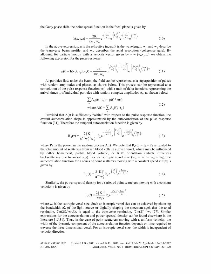
the Guoy phase shift, the point spread function in the focal plane is given by

22 2

22 2iyix iz

yx z 4πn22 2 i zww w λ

ix iy

2Kh(x, y, z) = e e e eπw w

− − − (10)

In the above expression, n is the refractive index, λ is the wavelength, wix and wiy describe the transverse beam profile, and wiz describes the axial resolution (coherence gate). By allowing for particle motion with a velocity vector given by v = (vx,vy,vz) we obtain the following expression for the pulse response:

( ) ( ) ( )

22 2y

x z22 2 ziyix iz

v tv t v t2 4πn2 2 i v tww w λx y z

ix iy

2Kp(t) = h(v t, v t, v t) = e e e eπw w

− − − (11)

As particles flow under the beam, the field can be represented as a superposition of pulses with random amplitudes and phases, as shown below. This process can be represented as a convolution of the pulse response function p(t) with a train of delta functions representing the arrival times tn of individual particles with random complex amplitudes An, as shown below:

n n

n

n nn

A p(t - t ) = p(t)*A(t)

where A(t) = A δ(t - t )

∑

∑ (12)

Provided that A(t) is sufficiently “white” with respect to the pulse response function, the overall autocorrelation shape is approximated by the autocorrelation of the pulse response function [31]. Therefore the temporal autocorrelation function is given by

( ) ( ) ( )

22 2y

x z22 2 ziyix iz

v τv τ v τ 4πn2 i v τww w λd A3/2 3/2 3/2

ix iy

2 | K |R (τ) = P e e e eπ w w

− − − (13)

where PA is the power in the random process A(t). We note that Rd(0) = Id ~ PA is related to the total amount of scattering from red blood cells in a given voxel, which may be influenced by either hematocrit, partial blood volume, or RBC orientation (which influences backscattering due to anisotropy). For an isotropic voxel size (wix = wiy = wiz = w0), the autocorrelation function for a series of point scatterers moving with a constant speed v = |v| is given by

2z

0

vτ 4πnv2 i τw λ

d A3/2 30

2 | K |R (τ) = P e eπ w

− (14)

Similarly, the power spectral density for a series of point scatterers moving with a constant velocity v is given by

22 2

0 z2

π w 2nv2 f -λv

d A20

2 | K |P (f) = P eπw v

− (15)

where w0 is the isotropic voxel size. Such an isotropic voxel size can be achieved by choosing the bandwidth Δλ of the light source or digitally shaping the spectrum such that the axial resolution, 2ln(2)λ2/πnΔλ, is equal to the transverse resolution, [2ln(2)]1/2w0 [27]. Similar expressions for the autocorrelation and power spectral density can be found elsewhere in the literature [15,31]. Thus, in the case of point scatterers moving with a uniform velocity, the width of the dynamic component of the autocorrelation function depends on time required to traverse the three-dimensional voxel. For an isotropic voxel size, the width is independent of velocity direction.


Model 2

While the preceding theory is valid for isotropic point particles traversing the resolution voxel, red blood cells are large, anisotropic scattering particles. We assume that, due to the finite extent of the red blood cell, the backscattered field from a red blood cell can be characterized by a spatial autocorrelation function. The extent of the spatial autocorrelation function is not greater than twice the RBC diameter, which is approximately 6-7 µm. The temporal autocorrelation can be obtained from the spatial autocorrelation by making the variable substitutions x = vxτ, y = vyτ, and z = vzτ:

x y z

d RBC x=v τ,y=v τ,z=v τR (τ) = R (x, y, z) (16)

Therefore, assuming the characteristics of the spatial autocorrelation do not change appreciably as RBCs move faster, higher RBC speeds will lead to shorter temporal autocorrelation widths.

Other effects

In reality, RBCs are highly anisotropic scattering particles with a distribution of sizes. Any dispersion in the backscattered field phase or amplitude during the particle transit time (~w0/v) will lead to additional decorrelation that is not accounted for in Model 1. Hence the above models are oversimplified and may not adequately represent RBC dynamics. Other effects that may influence the autocorrelation function decay include RBC diffusion [32], rotation [32], a random or time-varying RBC velocity distribution, and RBC membrane fluctuations [33]. Therefore, we view the above models as plausible but non-exhaustive justifications for a relationship between autocorrelation width and observed red blood cell dynamics. Due to the extreme complexity of these effects, we adopt a non-parametric, empirical approach. We propose to use the time scale of random fluctuations as a metric of capillary velocity, which we correlate against direct velocity measurements obtained via two-photon microscopy.

2.7. Data processing

The models developed above were used to motivate and guide the data processing. In this work we utilize the width of the power spectral density to quantify RBC velocity in capillaries in the rat neocortex. The scanning protocol samples each location in a 3D volume M = 100 times, at intervals of T = 7 milliseconds. This generates a 4-dimensional spatiotemporal data set A(x,y,z,t), where A is the complex OCT signal. The sampling interval of 7 milliseconds led to a Nyquist frequency of 71.4 Hz. As discussed below, aliasing in the power spectral density estimate is a limitation of the current technique. Currently the sampling interval of 7 milliseconds is limited by the camera line rate of 47 kHz and the time required for the galvanometer return at the end of the sawtooth waveform. Optimized galvanometer control and faster line scan cameras will enable reduction of the sampling interval in the future.

Based on data from the above scanning protocol, we perform a voxel-wise power spectral density estimate. The power spectral density estimate is calculated from the Fourier transformation of the complex autocorrelation function, calculated up to a temporal lag of 56 milliseconds, or N = 8 samples. As shown in Fig. 2(a), the width of the dynamic component of the autocorrelation function (Δτ) is assumed to be inversely proportional to velocity. Similarly, as shown in Fig. 2(b), the width of the dynamic component of the power spectral density (Δf) is assumed to be proportional to velocity. However, in order to estimate the width of the dynamic scattering component, it is necessary to first isolate the dynamic from the static component. Separation of the static and dynamic scattering components represents a challenge for which multiple solutions exist. One solution is to approximate the static component as the portion of the autocorrelation which does not decorrelate, R(τ>>Δτ), as


shown in Fig. 2(a). Another solution is fitting [34]. Yet another solution is to apply a temporal high-pass filter to the OCT data to remove the static scattering component.

18 Hz

45 Hz

z = 210 µm0.1 mm

0.1 mm

12

34

0.1 mm -50 0 500

0.2

0.4

0.6

0.8

1

τ (ms)

|R(τ)|∆f

1= 36.1 Hz

∆f2

= 27.9 Hz

∆f3

= 31.6 Hz

∆f4

= 23.8 Hz

A B

C E

D

C D

A

B

^

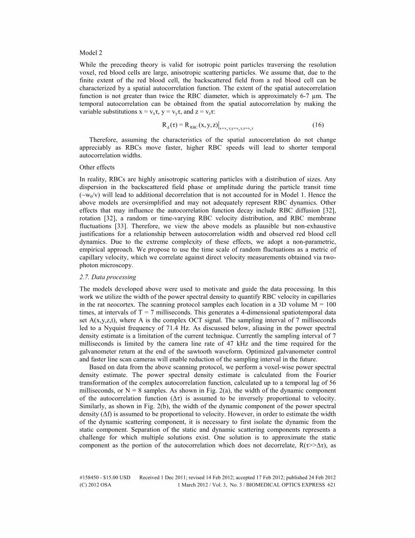
Fig. 3. Examples of autocorrelation function estimates from vasculature. En face OCT angiogram of the rat somatosensory cortex through a cranial window. (b) OCT Δf map, showing bandwidth in color scale. Cross-sectional slice through the angiogram (c) and Δf map (d) are shown, along with 4 labeled points where the autocorrelation function is estimated. (e) Plot of autocorrelation function estimate magnitudes at the 4 labeled points. The Δf values shown in the legend are proportional to the rate of autocorrelation decay.

For this work, we calculate the width of the power spectral density (Δf) using the following procedure. First, we calculate the autocorrelation function estimate as shown below. For the scan protocol we have chosen, M = 100, T = 7 milliseconds, and N = 8:

M-n-1*

corrx z m=0

A [x, y, z, mT]A [x, y, z, (m + n)T]R(x, y, z, nT) = for n = 0..., N -1, N

M - n

∑∑∑ (17)

A(x,y,z,t) is the four-dimensional complex-valued OCT signal. Each (x,y,z) location is sampled 100 times at intervals of 7 milliseconds in order to estimate the autocorrelation function. The subscript “corr” in the summation indicates that axial motion correction has been performed on the (m + n)th frame with respect to the mth frame for each (x,y) position [17]. “*” denotes complex conjugation. To ensure that the autocorrelation function estimate is Hermetian, we impose the following constraint:

*ˆ ˆR(x, y, z, nT) = R (x, y, z, -nT) for n = -N,-N +1,..., -1 (18)

We approximate the autocorrelation of the dynamic component by subtracting the static scattering component from the estimated autocorrelation function:

d sˆ ˆ ˆR (x, y, z, nT) = R(x, y, z, nT) - I (x, y, z) (19)

Our goal is to determine the time scale of fluctuations of the dynamic scattering component. While there are many approaches, here we calculate the power spectral density


estimate via discrete Fourier transformation. We use the absolute value of the autocorrelation function estimate to calculate the power spectral density estimate. By taking the absolute value of the autocorrelation function, we “demodulate” the power spectrum and ensure that any Doppler shift does not affect the width calculation. This guarantees that the power spectral density estimate is real and even:

N

d,demod dn=-N

ˆ ˆP (x, y, z, f) = |R (x, y, z, nT) | exp[-i2πf(nT)]∑ (20)

From our power spectral density estimate we calculate the frequency bandwidth, Δf, as follows:

d,demod

f

d,demodf

ˆ|f | P (x, y, z, f)Δf =

P (x, y, z, f)

∑∑

(21)

The power spectral density is calculated from the complex field autocorrelation function, and therefore Δf characterizes the complex field autocorrelation. This contrasts with previous work, where the intensity autocorrelation function was used [28].

-20 -10 0 10 20

30

35

40

µm

Hz

B

C

D

E

D

C

E

A

∆f

0.1 mm 0.1 mm

50 Hz

35 Hz

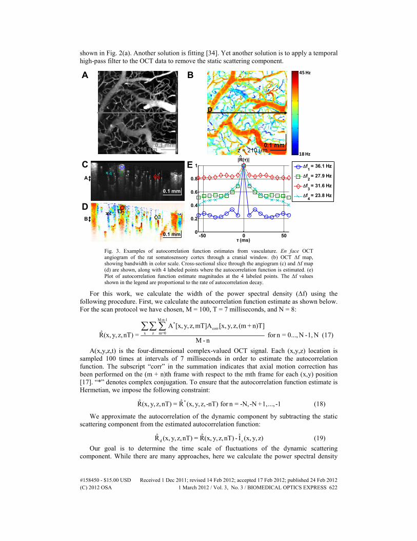
Fig. 4. OCT velocimetry of the rat somatosensory cortex. (a) En face OCT angiogram of the rat somatosensory cortex through a cranial window. (b) OCT Δf map, showing bandwidth in color scale. (c-d) Zoom of branch points show heterogeneous, branch-specific dynamics. (e) Cross-section through a vein shows increased bandwidth at the center, as would be expected from a parabolic profile.

3. Results

Figure 3(a) shows a conventional OCT angiogram, calculated from the following equation:

M-3

corrm=0

ΔA[x, y, z] = |A[x, y, z,mT]- A [x, y, z, (m + 2)T]|∑ (22)


The subscript “corr” in the summation indicates that axial motion correction has been performed on the (m + 2)nd frame with respect to the mth frame for each (x,y) position [17]. The angiogram was displayed after normalization to compensate attenuation and averaging over a depth range of 90 µm near the focus. Figure 3(b) shows the Δf map, similarly averaged over a depth range of 90 µm near the focus. The transparency of this image was set pixel-wise by a sigmoid function (with an empirically determined width and threshold) of the OCT angiogram shown in Fig. 3(a). Figure 3(c) shows a cross-sectional OCT angiogram with 4 points located within blood vessels. Points 1 and 2 are located in a pial vein, whereas points 3 and 4 are located in smaller parenchymal vessels. Figure 3(d) shows the Δf map with the same 4 points labeled. The absolute values of the autocorrelation function estimates at these points are plotted in Fig. 3(e), with calculated power spectral density widths (Δfi, i = 1,2,3,4) in the legend. It is important to note that while the point at the center of the large vessel (1) almost completely decorrelates over time, the other points (2-4) do not completely decorrelate. This is due to different relative amounts of static and dynamic scattering (Fig. 2). Point 1 is dominated by dynamic scattering, and point 3 is dominated by static scattering. Locations at the center of capillaries in the parenchyma may contain larger contributions of static scattering from the capillary endothelium, pericytes, and nearby cells. In addition, light that is forward scattered multiple times from static structures may contribute to the static scattering component. Additionally, hematocrit is lower is parencyhmal capillaries; this may reduce the dynamic scattering component relative to that in larger vessels.

Figure 4 shows examples of branch-specific dynamics. Figure 4(a) shows an OCT angiogram, averaged over a depth range of 30 µm near the focus. Figure 4(b) shows the Δf map, similarly averaged over a depth range of 30 µm near the focus. In Fig. 4(b), Δf values are spatially heterogenous, but clearly not random. Notably, values of Δf, as depicted in the color map, are consistent within non-branching segments of a single vessel, but often change dramatically after branch points. Numerous examples of this are evident in Fig. 4(b). Two examples of converging venular flow are shown in more detail. In Fig. 4(c), a smaller venule joins a large pial vein; the dynamics in the large pial vein do not appear to change dramatically before and after the smaller venule. However, Fig. 4(d) shows two veins of comparable size joining to form a larger vein. In this case, the dynamics in each converging vein are distinct, and furthermore, are different than dynamics in the larger vein after the branch point. Arteries and veins were distinguished based on branching pattern and morphology. Figure 4(e) shows the Δf profile across a surface pial vein. As expected, Δf increases at the center of the vessel. However, Δf does not go to zero at the edge of the vessel, while velocity should be zero at the edge of the vessel. This inaccuracy represents a limitation of our method, and is related to biases in the estimation procedure, the finite observation time, shot noise, and in vivo motion-induced decorrelation noise.

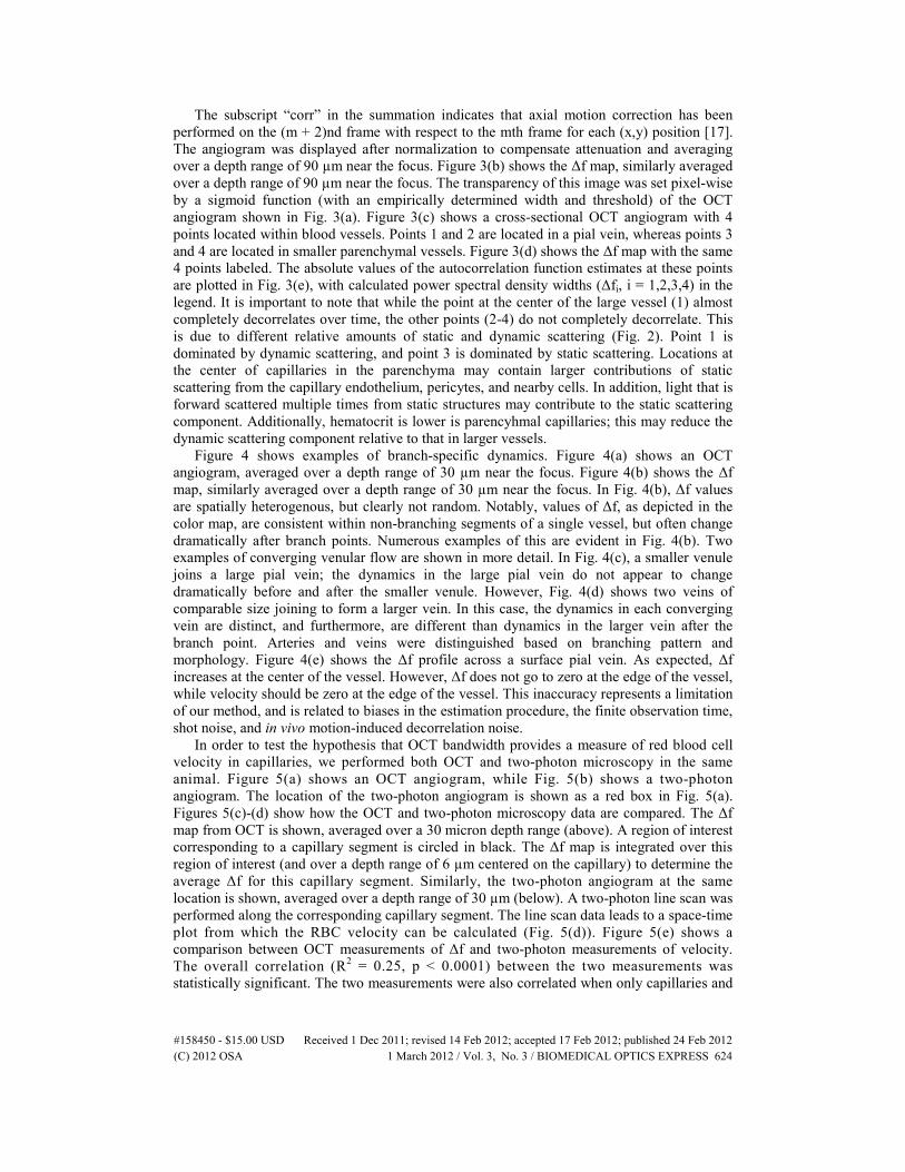
In order to test the hypothesis that OCT bandwidth provides a measure of red blood cell velocity in capillaries, we performed both OCT and two-photon microscopy in the same animal. Figure 5(a) shows an OCT angiogram, while Fig. 5(b) shows a two-photon angiogram. The location of the two-photon angiogram is shown as a red box in Fig. 5(a). Figures 5(c)-(d) show how the OCT and two-photon microscopy data are compared. The Δf map from OCT is shown, averaged over a 30 micron depth range (above). A region of interest corresponding to a capillary segment is circled in black. The Δf map is integrated over this region of interest (and over a depth range of 6 µm centered on the capillary) to determine the average Δf for this capillary segment. Similarly, the two-photon angiogram at the same location is shown, averaged over a depth range of 30 µm (below). A two-photon line scan was performed along the corresponding capillary segment. The line scan data leads to a space-time plot from which the RBC velocity can be calculated (Fig. 5(d)). Figure 5(e) shows a comparison between OCT measurements of Δf and two-photon measurements of velocity. The overall correlation (R2 = 0.25, p < 0.0001) between the two measurements was statistically significant. The two measurements were also correlated when only capillaries and


0.5 1 1.5 2 2.5 3

35

40

45

velocity (mm / s)

∆f (H

z)artery (A)capillary (C)vein (V)linear fit (C & V only)

0.1 mm

BA

EC

BC

r

1/v

t

0.1 mm

two-photon

two-photon

OCT

OCT

D

D

Fig. 5. Comparison of OCT and two photon velocimetry. (a) OCT angiogram and (b) two-photon angiogram. The location of the two-photon angiogram is shown as a red box in (a). (c) OCT Δf map at the location of the red box in (b). with a capillary (above, black region-of-interest) and two-photon line scan (below, red arrow) at the same location. (d) The slope of the space-time plot from the line scan is inversely proportional to the velocity (e) Comparison of velocity measured by two-photon microscopy and Δf values measured by OCT at the same location. The black line shows a linear fit for capillaries and veins only.

veins were considered (R2 = 0.25, p < 0.0001), and when only veins alone were considered (R2 = 0.51, p < 0.001). It should be noted that the large vessel (artery and vein) measurements were not necessarily performed at the center of the vessel. We attribute a significant portion of the variability between OCT and two-photon microscopy measurements to the fact that the measurements were not simultaneous, and we attribute nonlinearities in the relationship to aliasing. The offset in the relationship between Δf and velocity may be attributed to shot noise, in vivo motion-induced decorrelation noise, and biases in the estimation procedure, which increase the estimated power spectrum bandwidth.

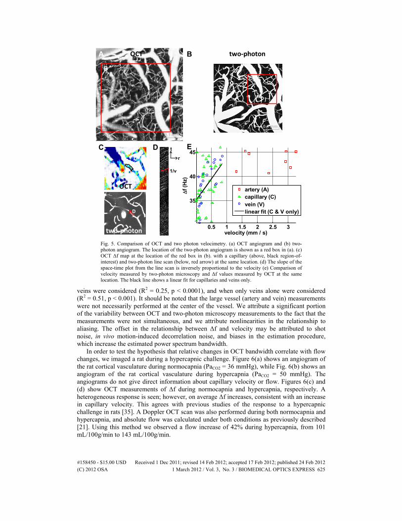
In order to test the hypothesis that relative changes in OCT bandwidth correlate with flow changes, we imaged a rat during a hypercapnic challenge. Figure 6(a) shows an angiogram of the rat cortical vasculature during normocapnia (PaCO2 = 36 mmHg), while Fig. 6(b) shows an angiogram of the rat cortical vasculature during hypercapnia (PaCO2 = 50 mmHg). The angiograms do not give direct information about capillary velocity or flow. Figures 6(c) and (d) show OCT measurements of Δf during normocapnia and hypercapnia, respectively. A heterogeneous response is seen; however, on average Δf increases, consistent with an increase in capillary velocity. This agrees with previous studies of the response to a hypercapnic challenge in rats [35]. A Doppler OCT scan was also performed during both normocapnia and hypercapnia, and absolute flow was calculated under both conditions as previously described [21]. Using this method we observed a flow increase of 42% during hypercapnia, from 101 mL/100g/min to 143 mL/100g/min.


z = 420 µm0.1 mm

B

D

hypercapnia

36 Hz

18 Hz

z = 420 µm0.1 mm

A

C

normocapnia

Fig. 6. Capillary velocimetry during a hypercapnic challenge. OCT angiograms under normocapnia (a) and hypercapnia (b) show no noticeable differences. However, OCT Δf map shows an apparent redistribution of capillary velocity during hypercapnia (d) compared to normocapnia (c). On average, the number of high-velocity capillaries is increased during hypercapnia.

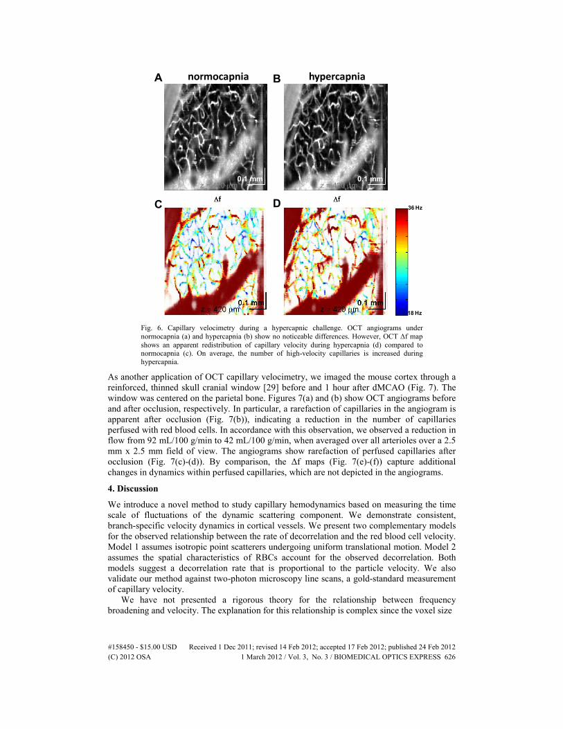
As another application of OCT capillary velocimetry, we imaged the mouse cortex through a reinforced, thinned skull cranial window [29] before and 1 hour after dMCAO (Fig. 7). The window was centered on the parietal bone. Figures 7(a) and (b) show OCT angiograms before and after occlusion, respectively. In particular, a rarefaction of capillaries in the angiogram is apparent after occlusion (Fig. 7(b)), indicating a reduction in the number of capillaries perfused with red blood cells. In accordance with this observation, we observed a reduction in flow from 92 mL/100 g/min to 42 mL/100 g/min, when averaged over all arterioles over a 2.5 mm x 2.5 mm field of view. The angiograms show rarefaction of perfused capillaries after occlusion (Fig. 7(c)-(d)). By comparison, the Δf maps (Fig. 7(e)-(f)) capture additional changes in dynamics within perfused capillaries, which are not depicted in the angiograms.

4. Discussion

We introduce a novel method to study capillary hemodynamics based on measuring the time scale of fluctuations of the dynamic scattering component. We demonstrate consistent, branch-specific velocity dynamics in cortical vessels. We present two complementary models for the observed relationship between the rate of decorrelation and the red blood cell velocity. Model 1 assumes isotropic point scatterers undergoing uniform translational motion. Model 2 assumes the spatial characteristics of RBCs account for the observed decorrelation. Both models suggest a decorrelation rate that is proportional to the particle velocity. We also validate our method against two-photon microscopy line scans, a gold-standard measurement of capillary velocity.

We have not presented a rigorous theory for the relationship between frequency broadening and velocity. The explanation for this relationship is complex since the voxel size


PAL

S0.1 mm

A B

C D

PAL

S0.1 mm

Pre-dMCAO 1 hour Post-dMCAO

E F

C,ED,F

MCAMCA

0.1 mm

0.1 mm

38 Hz18 Hz

Fig. 7. OCT methods of velocimetry provide additional insight which is not obtained from conventional OCT angiograms. OCT angiograms of the mouse cortex before (a) and one day after (b) distal MCA occlusion are shown. Surface vessels (pial and dural) have been colored yellow, while deeper vessels are colored in green. Black and white OCT angiograms show a rarefaction of perfused capillaries after occlusion (d) compared to before occlusion (c). OCT Δf maps show a reduction in velocity in perfused capillaries after occlusion (f) compared to before occlusion (e). The Δf maps (e-f) provide novel information which is not contained in the angiograms (c-d), and show an increase in heterogeneity after stroke.

(~3.6 x 3.6 x 3.6 µm) is on the order of the size of an RBC (6.5 x 6.5 x 1.5 µm). Therefore, we can identify two effects which lead to field fluctuations as red blood cells traverse the voxel. Firstly, as one red blood cell is replaced by another red blood cell with a different, random orientation and axial position, the field amplitude and phase will change randomly. Secondly, for a single red blood cell traversing a voxel, we expect that amplitude and phase fluctuations will result, due to the irregular red blood cell size and random orientation, as well as a random velocity axial projection distribution. The first effect, described by Model 1, is related to speckle decorrelation described earlier [15], and should be independent of the direction of flow, since the voxel is isotropic. The second effect, described in part by Model 2, is related to the spatial characteristics of the RBCs. However, the quantitative description of decorrelation caused by red blood cell dynamics is complex due to the highly anisotropic scattering from red blood cells [36], membrane fluctuations [33], deformations [37], and orientation changes and is beyond the scope of this paper.

Previously, validation of OCT velocity measurements were performed in scattering flow phantoms. Representative ex vivo phantoms that simulate capillary flow dynamics are challenging to fabricate. Furthermore, red blood cell density and velocity in a real microvascular network are complicated and difficult to measure directly [38], and challenging to replicate in an in vitro experiment. In this work, rather than attempt to perform ex vivo validation, we compared OCT capillary measurements with two-photon microscopy line scans, which have been the gold standard for measurements of capillary velocity since their


introduction in 1998 [16]. Our validation study required imaging the same animals on both a two-photon microscope and an OCT microscope. While we minimized the time between imaging sessions and attempted to maintain physiology, we acknowledge that our validation experiment had limitations. Nevertheless, the data shows that OCT measures of Δf positively correlate with two-photon microscopy measurements of velocity, when compared across vessels. Of note, OCT Δf measurements correlated with velocities ranging from 0 to 1 mm / s (Fig. 5(e)), which fall below the measurable dynamic range of current high-speed Doppler OCT systems [39].

Power spectrum measurements similar to those presented here are used for laser Doppler imaging. There are several differences between our imaging method and laser Doppler. Firstly, in laser Doppler imaging, due to the source-detector geometry, light has scattered multiple times before detection, it is not possible to unambiguously relate the bandwidth to velocity or flow [40]. Therefore baseline measurements of laser Doppler bandwidth cannot be compared across subjects. In contrast, for the method presented here, provided that mostly single scattered light is detected within the OCT voxel, and the method for removing static scattering is effective, the bandwidth Δf can be directly related to velocity. Our validation against two-photon microscopy supports this hypothesis. Furthermore, although not directly shown here, it is reasonable to hypothesize that the degree of broadening, quantified by Δf, can be compared across subjects. As our technique is phase-sensitive and therefore requires high mechanical stability of the sample, one possible factor confounding intersubject comparisons is different severities of motion artifacts in different animals.

4.1. Application to retinal imaging

We anticipate that velocimetry techniques could be used in retinal imaging to assess dynamics of capillary perfusion. In particular, performing analysis along the slow axis of repeated B-scans enables parallelization of measurements and reduced overall imaging times [20,21,24]. It is possible to maintain correlation across multiple rapidly acquired images in the human retina in vivo, as this is a prerequisite for phase variance imaging [41]. In addition, to reduce sensitivity to motion, the intensity autocorrelation could be used to assess the degree of capillary perfusion, provided that an appropriate model is developed for its interpretation.

4.2. Limitations and future work

Although our technique has shown promise, there are several limitations of our current method. The time required for estimation of autocorrelation width is necessarily longer than either Doppler OCT or OCT angiography, both of which require a minimum of only two axial scans at the same transverse location. This can be qualitatively understood from the fact that estimation of the standard deviation of a distribution is necessarily less precise than estimation of the centroid of a distribution. Performing analysis along the slow axis of repeated B-scans reduces the scan time through parallelization and improves efficiency of data acquisition. However, the resulting undersampling may result in aliasing; thus, at the speeds demonstrated here, this method is currently not suitable for measuring voxels with fast decorrelation rates, such as voxels with arterial flow. In fact, the nonlinear relationship between Δf and velocity in Fig. 5(e) is likely due to aliasing.

We have also not investigated the effects of defocus or multiple scattering on our measurements. Since the decorrelation rate depends on the voxel size, according to Model 1, one expects that for a given velocity, the rate of decorrelation will decrease at depths away from the focal plane where the transverse resolution is worse. However, at increased depths one also expects that multiple scattering will increase the rate of decorrelation. Thus, for a given velocity, the rate of decorrelation decreases superficially to the focal plane, while deeper than the focal plane the behavior is less well defined.


Lastly, our technique of width estimation is ad hoc and is likely to be biased and inefficient. Therefore, we anticipate that parametric estimation techniques will improve performance in the future.

5. Conclusion

In conclusion, we have demonstrated a method for capillary velocimetry in highly scattering tissue with OCT. The method requires, firstly, isolation of the dynamic scattering component from the static scattering component, and secondly, characterization of the time scale of random fluctuations of the dynamic scattering component. Improved efficiency of data acquisition is achieved by performing analysis along the slow axis of repeated B-scans at the same transverse location. In this work, we use the power spectrum bandwidth to characterize the dynamic scattering component, although alternative analyses based on the autocorrelation function are possible. The bandwidth correlates with velocity measured by two-photon microscopy line scans in the range from 0 to 1 mm / s, and has the expected behavior under a hypercapnic challenge and during distal middle cerebral artery occlusion. Therefore, techniques of capillary velocimetry may provide information complementary to Doppler OCT and OCT angiography techniques.

Acknowledgments

We acknowledge support from the National Institutes of Health (R00NS067050, NS055104, EB001954 R01), the American Heart Association (11IRG5440002), and the Glaucoma Research Foundation Catalyst for a Cure 2. We thank Maria Angela Franceschini for permission to use the OCT system.


Documents

OCT methods for capillary velocimetry