Embed Size (px)
Citation preview
PNNL-16626
Development of Millimeter-Wave Velocimetry and Acoustic Time-of-Flight Tomography for Measurements in Densely Loaded Gas-Solid Riser Flow A Final Report for the Multiphase Fluid Dynamics Research Consortium J.A. Fort D.M. Pfund D.M. Sheen R.A. Pappas G.P. Morgen April 2007 Prepared for the U.S. Department of Energy under Contract DE-AC05-76RL01830
PNNL-16626
Development of Millimeter-Wave Velocimetry and Acoustic Time-of-Flight Tomography for Measurements in Densely Loaded Gas-Solid Riser Flow A Final Report for the Multiphase Fluid Dynamics Research Consortium J.A. Fort D.M. Pfund D.M. Sheen R.A. Pappas G.P. Morgen April 2007 Prepared for the U.S. Department of Energy under Contract DE-AC05-76RL01830 Pacific Northwest National Laboratory Richland, Washington 99352
MFDRC
iii
Summary
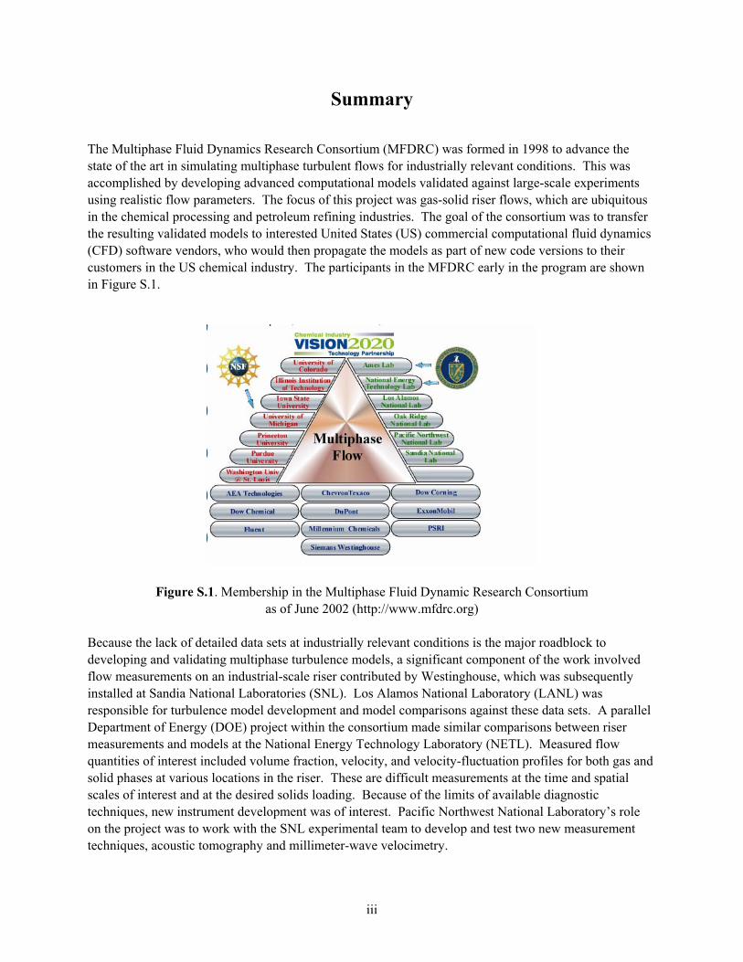
The Multiphase Fluid Dynamics Research Consortium (MFDRC) was formed in 1998 to advance the state of the art in simulating multiphase turbulent flows for industrially relevant conditions. This was accomplished by developing advanced computational models validated against large-scale experiments using realistic flow parameters. The focus of this project was gas-solid riser flows, which are ubiquitous in the chemical processing and petroleum refining industries. The goal of the consortium was to transfer the resulting validated models to interested United States (US) commercial computational fluid dynamics (CFD) software vendors, who would then propagate the models as part of new code versions to their customers in the US chemical industry. The participants in the MFDRC early in the program are shown in Figure S.1.
Figure S.1. Membership in the Multiphase Fluid Dynamic Research Consortium as of June 2002 (http://www.mfdrc.org)
Because the lack of detailed data sets at industrially relevant conditions is the major roadblock to developing and validating multiphase turbulence models, a significant component of the work involved flow measurements on an industrial-scale riser contributed by Westinghouse, which was subsequently installed at Sandia National Laboratories (SNL). Los Alamos National Laboratory (LANL) was responsible for turbulence model development and model comparisons against these data sets. A parallel Department of Energy (DOE) project within the consortium made similar comparisons between riser measurements and models at the National Energy Technology Laboratory (NETL). Measured flow quantities of interest included volume fraction, velocity, and velocity-fluctuation profiles for both gas and solid phases at various locations in the riser. These are difficult measurements at the time and spatial scales of interest and at the desired solids loading. Because of the limits of available diagnostic techniques, new instrument development was of interest. Pacific Northwest National Laboratory’s role on the project was to work with the SNL experimental team to develop and test two new measurement techniques, acoustic tomography and millimeter-wave velocimetry.
iv
Acoustic tomography is a promising technique for gas-solid flow measurements in risers and PNNL has substantial related experience in this area. PNNL is also active in developing millimeter wave imaging techniques and this technology presents an additional approach to make desired measurements. PNNL supported the advanced diagnostics development part of this project by evaluating these techniques, and then by adapting and developing the selected technology to bulk gas-solids flows and by implementing them for testing in the SNL riser testbed. During the course of this project, millimeter wave velocimetry was demonstrated in the SNL riser as being capable of making local measurements of solid phase velocities. These measurements were made through the acrylic riser wall and included a range of particle concentrations from 0.1 to 5%. The measurement signal is a spectrum of Doppler shifted frequencies, where the peak magnitude indicates bulk velocity magnitude. Measurements at concentrations up to 20% were attempted, but the bulk axial velocity was not distinguishable from the measurement. Potential exists for measuring turbulence quantities within the sampling volume, but this requires further work to characterize and extract this information from the measured spectrum. Finally, while our measurements focused on axial particle velocity, other velocity components can be resolved by reorienting antennas and simultaneous measurement of three components could be done with replicated instruments. Acoustic tomography presented a greater challenge. At the completion of this project, a prototype four-transducer system was demonstrated in the SNL riser. This four-transducer system represents the minimum building block for a complete tomographic array. Realizing the potential of such a system requires further development in transducer design to give good performance over wider angles with large bandwidth.
v
Acknowledgments
This work was sponsored by the US Department of Energy, Energy Efficiency and Renewable Energy (EERE), Office of Industrial Technology Programs. The authors would like to acknowledge the initiative and support of Brian Valentine of DOE-ITP, without which the MFDRC would not have been founded nor carried out its work. We acknowledge Tyler Thompson, DOW Chemical, for his leadership of the MFDRC and promotion of the MFDRC within the Chemical and Petrochemical process community. We acknowledge the many MFDRC participants and team members that made this a rich and unique collaboration, from DOE national laboratories, from academia, from chemical and petrochemical industry, and from commercial CFD companies,
We acknowledge Steve Weiner and Wally Weimer, PNNL for their support of this project and for support of the early committee work that preceded it. Finally, we wish to thank the contributions of the many PNNL staff who made significant contributions to this project: Tom Kiefer for detailed design and production of the multi-acoustic ultrasonic processor (AUP), Mike Fleming for development of the LabVIEW interface to the millimeter-wave instrument, Jerry Posakony and Mathew Flake for the ultrasonic transducer design and testing, and Mike White for the layout of the wave guides for the final configuration design of the riser section traverse and window for the millimeter-wave.

vii
Contents
1.0 Introduction ...................................................................................................................................... 1.1
2.0 Test Facilities ................................................................................................................................... 2.1
2.1 PNNL Riser ............................................................................................................................ 2.1
2.2 SNL Riser ............................................................................................................................... 2.2
3.0 Millimeter-Wave Velocimetry ......................................................................................................... 3.1
3.1 Design of Instrument .............................................................................................................. 3.1
3.2 Demonstration Tests at SNL .................................................................................................. 3.2
3.3 Second Generation Prototype ................................................................................................. 3.5
4.0 Ultrasonic Tomography ................................................................................................................... 4.1
4.1 Approach ................................................................................................................................ 4.1
4.1.1 Flow Velocity ............................................................................................................ 4.1
4.2 Tomographic Reconstruction ................................................................................................. 4.1
4.3 Time-of-Flight Measurement ................................................................................................. 4.3
4.3.1 Multi-AUP Prototype ................................................................................................ 4.6
4.3.2 Multi-AUP Prototype Testing ................................................................................. 4.10
4.4 Transducer Development ..................................................................................................... 4.15
5.0 Conclusions and Recommendations................................................................................................. 5.1
5.1 Conclusions ............................................................................................................................ 5.1
5.2 Recommendations .................................................................................................................. 5.1
6.0 References ........................................................................................................................................ 6.1
Appendix: Description of Software Interface to Millimeter-Wave Instrument ....................................... A.1
viii
Figures
2.1 PNNL 5.1 cm Riser .........................................................................................................................2.1
2.2 SNL’s Pilot-Scale Circulating Fluidized Bed..................................................................................2.3
3.1 Schematic Diagram of Millimeter-Wave Doppler Transceiver.......................................................3.2
3.2 Millimeter-Wave Instrument Configuration During August 2001 Testing at SNL.........................3.2
3.3 Velocity Distributions near Center of Riser for Range of Solids Loadings ....................................3.3
3.4 Velocity Distributions at Four Positions across Riser Cross-Section..............................................3.4
3.5 Time Variation of Velocity near Riser Center.................................................................................3.4
3.6 Time Variation of Velocity Adjacent to Wall of Riser....................................................................3.5
3.7 Millimeter-Wave Instrument Head Setup for Direct Measurements of Axial Flow Velocity.........3.6
3.8 Turntable Test Configuration for Checking Velocity Measurements .............................................3.6
3.9 Doppler Frequency Distribution Obtained in Turntable Measurements .........................................3.7
3.10 Design Drawing for Foam Window Section ...................................................................................3.8
3.11 Turntable Test Configuration for Foam Sample Attenuation Measurements..................................3.8
3.12 Attenuation Results for General Plastics Foam Samples ................................................................3.9
4.1 Approach to TOF Tomography .......................................................................................................4.4
4.2 Examples of Velocity and Distribution Completed Using Tomographic........................................4.5
4.3 System Specifications and Detail of a Single Transceiver Board ...................................................4.7
4.4 Transceiver Board – One per Transducer........................................................................................4.8
4.5 Housing with Power Supply and Amps – Front ..............................................................................4.8
4.6 Housing with Power Supply and Amps – Rear ...............................................................................4.9
4.7 Modulus of Cross-Correlation of Transmitted Code with Received Baseband Waveform...........4.11
4.8 Repeatability of the TOF Measurement Was ± 2.5 μ s .................................................................4.12
4.9 Separate Versus Simultaneous Transmissions ..............................................................................4.12
4.10 Time-of-Flight Versus Solids Loading of FCC Catalyst ...............................................................4.13
ix
Tables
3.1 Test Conditions for 8/01 Millimeter-Wave Velocimeter Testing....................................................3.2
3.2 Test Parameters and Sample Results for 100 GHz Doppler Transceiver Characterization.............3.7
3.3 Instrument as Determined in Turntable Tests..................................................................................3.7
3.4 Properties of General Plastics FR6703 Used for Window Section .................................................3.9
4.1 Measured TOF Values in Flow Tests with Glass Beads ...............................................................4.14

xi
Acronyms and Abbreviations
AUP Acoustic ultrasonic processor
CFD Computational fluid dynamics
COTS Commercial off the shelf
dBm Power ratio in decibel (dB) referenced to 1 mW
EERE Energy Efficiency and Renewable Energy
FCC Fluid catalytic cracking
FIFO First in first out
FWHM Full width half max
HEPA High efficiency particulate air
ID Inner diameter
ITP Industrial Technology Program (Office of DOE-EERE)
LANL Los Alamos National Laboratory
MFDRC Multiphase Fluid Dynamics Research Consortium
mm millimeter
ms millisecond
NETL National Energy Technology Laboratory
OIT Office of Industrial Technology (forerunner of ITP)
PNNL Pacific Northwest National Laboratory
PVC polyvinyl/chloride
RF Radio frequency
SNL Sandia National Laboratories
TOF Time of flight
1.1
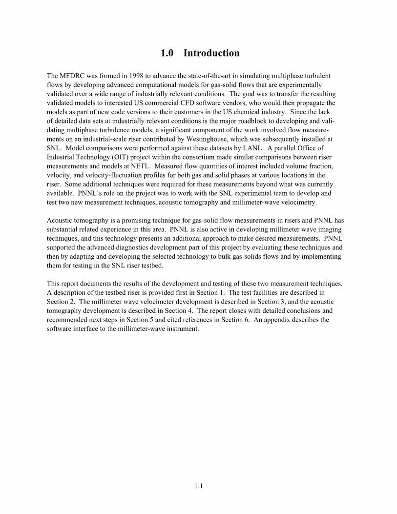
1.0 Introduction
The MFDRC was formed in 1998 to advance the state-of-the-art in simulating multiphase turbulent flows by developing advanced computational models for gas-solid flows that are experimentally validated over a wide range of industrially relevant conditions. The goal was to transfer the resulting validated models to interested US commercial CFD software vendors, who would then propagate the models as part of new code versions to their customers in the US chemical industry. Since the lack of detailed data sets at industrially relevant conditions is the major roadblock to developing and vali-dating multiphase turbulence models, a significant component of the work involved flow measure-ments on an industrial-scale riser contributed by Westinghouse, which was subsequently installed at SNL. Model comparisons were performed against these datasets by LANL. A parallel Office of Industrial Technology (OIT) project within the consortium made similar comparisons between riser measurements and models at NETL. Measured flow quantities of interest included volume fraction, velocity, and velocity-fluctuation profiles for both gas and solid phases at various locations in the riser. Some additional techniques were required for these measurements beyond what was currently available. PNNL’s role on the project was to work with the SNL experimental team to develop and test two new measurement techniques, acoustic tomography and millimeter-wave velocimetry. Acoustic tomography is a promising technique for gas-solid flow measurements in risers and PNNL has substantial related experience in this area. PNNL is also active in developing millimeter wave imaging techniques, and this technology presents an additional approach to make desired measurements. PNNL supported the advanced diagnostics development part of this project by evaluating these techniques and then by adapting and developing the selected technology to bulk gas-solids flows and by implementing them for testing in the SNL riser testbed. This report documents the results of the development and testing of these two measurement techniques. A description of the testbed riser is provided first in Section 1. The test facilities are described in Section 2. The millimeter wave velocimeter development is described in Section 3, and the acoustic tomography development is described in Section 4. The report closes with detailed conclusions and recommended next steps in Section 5 and cited references in Section 6. An appendix describes the software interface to the millimeter-wave instrument.
2.1
2.0 Test Facilities
2.1 PNNL Riser
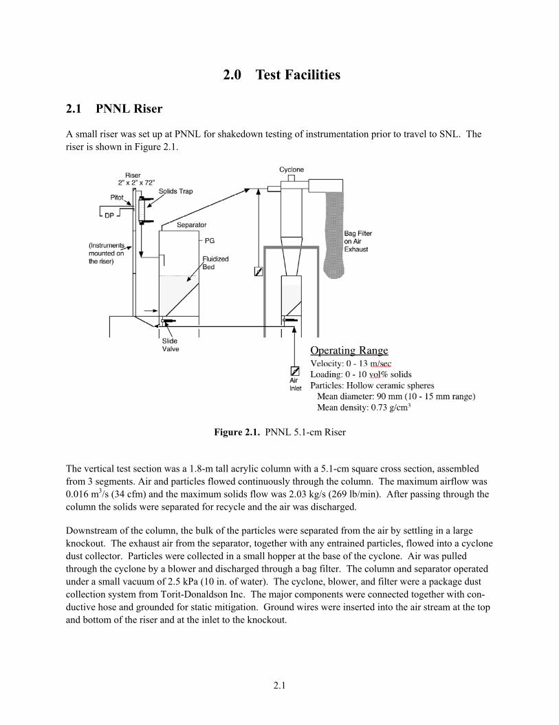
A small riser was set up at PNNL for shakedown testing of instrumentation prior to travel to SNL. The riser is shown in Figure 2.1.
Figure 2.1. PNNL 5.1-cm Riser
The vertical test section was a 1.8-m tall acrylic column with a 5.1-cm square cross section, assembled from 3 segments. Air and particles flowed continuously through the column. The maximum airflow was 0.016 m3/s (34 cfm) and the maximum solids flow was 2.03 kg/s (269 lb/min). After passing through the column the solids were separated for recycle and the air was discharged.
Downstream of the column, the bulk of the particles were separated from the air by settling in a large knockout. The exhaust air from the separator, together with any entrained particles, flowed into a cyclone dust collector. Particles were collected in a small hopper at the base of the cyclone. Air was pulled through the cyclone by a blower and discharged through a bag filter. The column and separator operated under a small vacuum of 2.5 kPa (10 in. of water). The cyclone, blower, and filter were a package dust collection system from Torit-Donaldson Inc. The major components were connected together with con-ductive hose and grounded for static mitigation. Ground wires were inserted into the air stream at the top and bottom of the riser and at the inlet to the knockout.
2.2
The system was designed to operate with hollow ceramic microspheres (from PQ Corporation) as the solid particle phase. The particles had a mean diameter of 90 μm, covering a range from 10 to 150 μm and a mean density of 0.73 g/cm3. The low density of the hollow particles allowed relatively large loadings of up to 10 vol% solids to be achieved. The system was sometimes operated with fluid catalytic cracking (FCC) catalyst particles (described in detail elsewhere in this report) as the solid phase, at much lower solids loading.
Ultrasonic and millimeter wave instruments were tested in the middle section of the column. A pitot tube was sometimes inserted into the upper section for measurements of airflow rate. A solids trap was posi-tioned between the riser and the knockout. The trap had quick operating values on the inlet and outlet and was intended for measurement of solids loading. Unfortunately, the trap proved difficult to operate; and there was no procedure for validating loading results from the trap.
2.2 SNL Riser
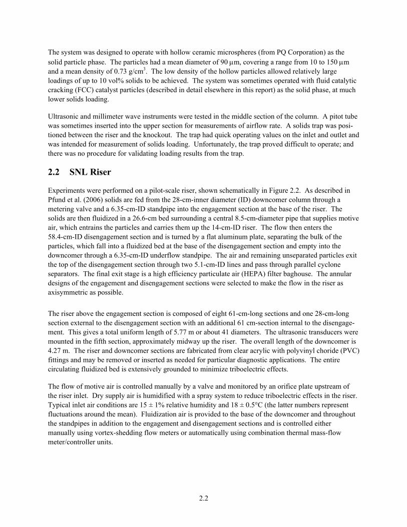
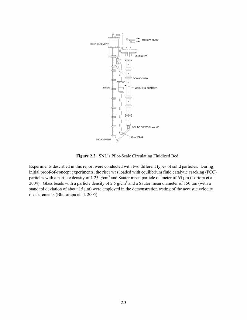
Experiments were performed on a pilot-scale riser, shown schematically in Figure 2.2. As described in Pfund et al. (2006) solids are fed from the 28-cm-inner diameter (ID) downcomer column through a metering valve and a 6.35-cm-ID standpipe into the engagement section at the base of the riser. The solids are then fluidized in a 26.6-cm bed surrounding a central 8.5-cm-diameter pipe that supplies motive air, which entrains the particles and carries them up the 14-cm-ID riser. The flow then enters the 58.4-cm-ID disengagement section and is turned by a flat aluminum plate, separating the bulk of the particles, which fall into a fluidized bed at the base of the disengagement section and empty into the downcomer through a 6.35-cm-ID underflow standpipe. The air and remaining unseparated particles exit the top of the disengagement section through two 5.1-cm-ID lines and pass through parallel cyclone separators. The final exit stage is a high efficiency particulate air (HEPA) filter baghouse. The annular designs of the engagement and disengagement sections were selected to make the flow in the riser as axisymmetric as possible.
The riser above the engagement section is composed of eight 61-cm-long sections and one 28-cm-long section external to the disengagement section with an additional 61 cm-section internal to the disengage-ment. This gives a total uniform length of 5.77 m or about 41 diameters. The ultrasonic transducers were mounted in the fifth section, approximately midway up the riser. The overall length of the downcomer is 4.27 m. The riser and downcomer sections are fabricated from clear acrylic with polyvinyl choride (PVC) fittings and may be removed or inserted as needed for particular diagnostic applications. The entire circulating fluidized bed is extensively grounded to minimize triboelectric effects.
The flow of motive air is controlled manually by a valve and monitored by an orifice plate upstream of the riser inlet. Dry supply air is humidified with a spray system to reduce triboelectric effects in the riser. Typical inlet air conditions are 15 ± 1% relative humidity and 18 ± 0.5°C (the latter numbers represent fluctuations around the mean). Fluidization air is provided to the base of the downcomer and throughout the standpipes in addition to the engagement and disengagement sections and is controlled either manually using vortex-shedding flow meters or automatically using combination thermal mass-flow meter/controller units.
2.3
DOWNCOMER
WEIGHING CHAMBER
BALL VALVE
CYCLONES
TO HEPA FILTER
SOLIDS CONTROL VALVE.
ENGAGEMENT
DISENGAGEMENT
RISER
Figure 2.2. SNL’s Pilot-Scale Circulating Fluidized Bed
Experiments described in this report were conducted with two different types of solid particles. During initial proof-of-concept experiments, the riser was loaded with equilibrium fluid catalytic cracking (FCC) particles with a particle density of 1.25 g/cm3 and Sauter mean particle diameter of 65 μm (Tortora et al. 2004). Glass beads with a particle density of 2.5 g/cm3 and a Sauter mean diameter of 150 μm (with a standard deviation of about 15 μm) were employed in the demonstration testing of the acoustic velocity measurements (Bhusarapu et al. 2005).
3.1
3.0 Millimeter-Wave Velocimetry
Millimeter-wave Doppler velocimetry is one of several possible means for measuring the velocity of particles within gas-solid flows. Millimeter-waves are high-frequency microwaves typically defined to cover the electromagnetic wavelength range of 1.0 mm to 10.0 mm. This range of wavelengths corre-sponds to a frequency range of 30 GHz to 300 GHz. Millimeter-waves are well suited for measurement applications involving gas-solid flows since the relatively long-wavelength waves can easily penetrate dense flows of small particles that are opaque to shorter wavelength laser-optical instruments.
The operating principle is the same as in laser Doppler velocimetry: incident electromagnetic radiation is Doppler shifted in frequency proportionate to the velocity of the scattering medium. The scattering medium in this case is the solid particulate. In contrast to laser Doppler velocimetry, the electromagnetic radiation in this case is much longer wavelength (close to that of microwave and radar) so that horn antennas are used in place of optical lenses. The measurement volume is illuminated with the source from the transmit antenna; a second antenna in the plane of the desired measurement is used to define the measurement volume and collect the scattered radiation.
The relationship between velocity and shifted frequency, fd, is
θsin2cvffd = (3.1)
where v is the particle velocity, f is the millimeter-wave frequency, c is the speed of light and θ is the angle between the transmit beam and particle flow. For a particle velocity of 1 meter/second and θ equal to 45 degrees, the expected Doppler frequencies is 452.5 Hz at 96 GHz.
3.1 Design of Instrument
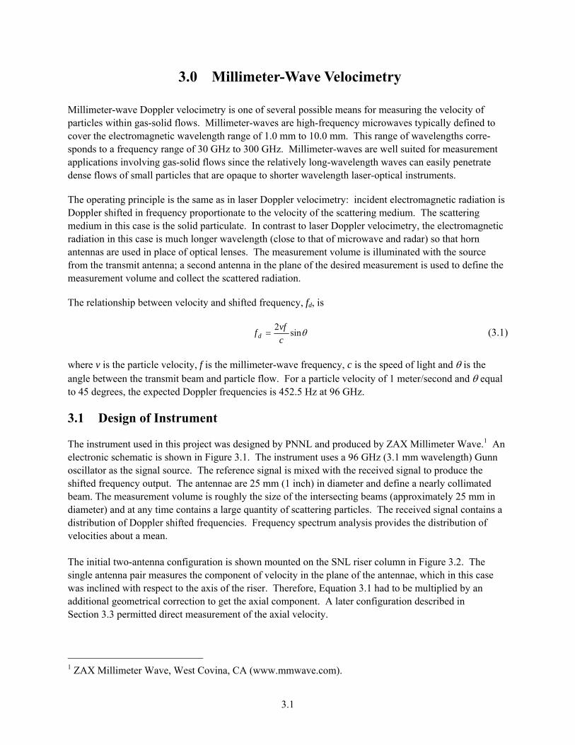
The instrument used in this project was designed by PNNL and produced by ZAX Millimeter Wave.1 An electronic schematic is shown in Figure 3.1. The instrument uses a 96 GHz (3.1 mm wavelength) Gunn oscillator as the signal source. The reference signal is mixed with the received signal to produce the shifted frequency output. The antennae are 25 mm (1 inch) in diameter and define a nearly collimated beam. The measurement volume is roughly the size of the intersecting beams (approximately 25 mm in diameter) and at any time contains a large quantity of scattering particles. The received signal contains a distribution of Doppler shifted frequencies. Frequency spectrum analysis provides the distribution of velocities about a mean. The initial two-antenna configuration is shown mounted on the SNL riser column in Figure 3.2. The single antenna pair measures the component of velocity in the plane of the antennae, which in this case was inclined with respect to the axis of the riser. Therefore, Equation 3.1 had to be multiplied by an additional geometrical correction to get the axial component. A later configuration described in Section 3.3 permitted direct measurement of the axial velocity.
1 ZAX Millimeter Wave, West Covina, CA (www.mmwave.com).
3.2
I = A cos(2π fd t+φ)
T
R
Oscillator
Mixer
Figure 3.1. Schematic Diagram of Millimeter-Wave Doppler Transceiver
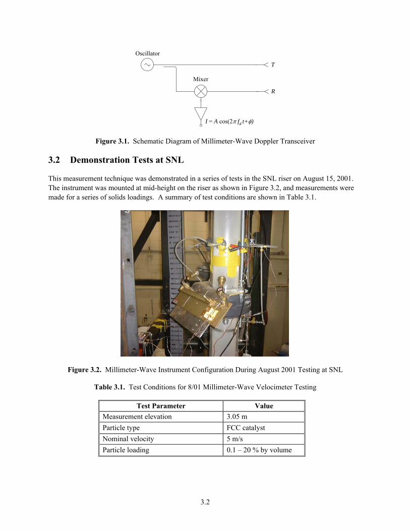
3.2 Demonstration Tests at SNL
This measurement technique was demonstrated in a series of tests in the SNL riser on August 15, 2001. The instrument was mounted at mid-height on the riser as shown in Figure 3.2, and measurements were made for a series of solids loadings. A summary of test conditions are shown in Table 3.1.
Figure 3.2. Millimeter-Wave Instrument Configuration During August 2001 Testing at SNL
Table 3.1. Test Conditions for 8/01 Millimeter-Wave Velocimeter Testing
Test Parameter Value Measurement elevation 3.05 m Particle type FCC catalyst Nominal velocity 5 m/s Particle loading 0.1 – 20 % by volume
3.3
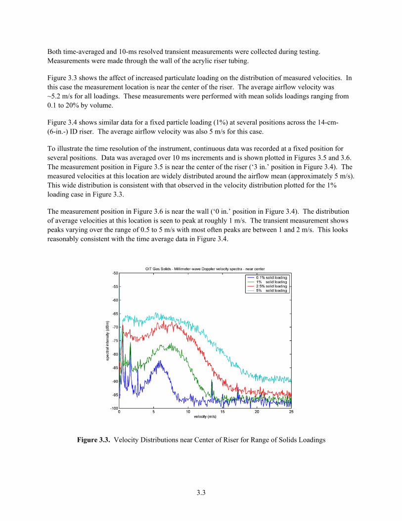
Both time-averaged and 10-ms resolved transient measurements were collected during testing. Measurements were made through the wall of the acrylic riser tubing.
Figure 3.3 shows the affect of increased particulate loading on the distribution of measured velocities. In this case the measurement location is near the center of the riser. The average airflow velocity was ~5.2 m/s for all loadings. These measurements were performed with mean solids loadings ranging from 0.1 to 20% by volume.
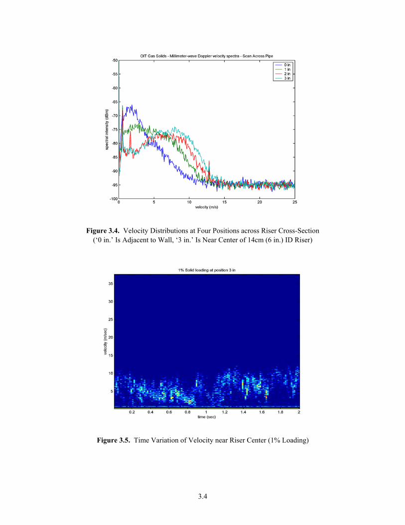
Figure 3.4 shows similar data for a fixed particle loading (1%) at several positions across the 14-cm- (6-in.-) ID riser. The average airflow velocity was also 5 m/s for this case.
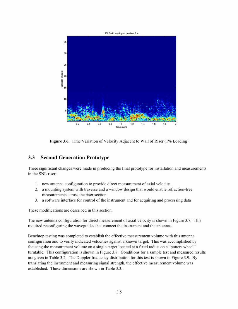
To illustrate the time resolution of the instrument, continuous data was recorded at a fixed position for several positions. Data was averaged over 10 ms increments and is shown plotted in Figures 3.5 and 3.6. The measurement position in Figure 3.5 is near the center of the riser (‘3 in.’ position in Figure 3.4). The measured velocities at this location are widely distributed around the airflow mean (approximately 5 m/s). This wide distribution is consistent with that observed in the velocity distribution plotted for the 1% loading case in Figure 3.3.
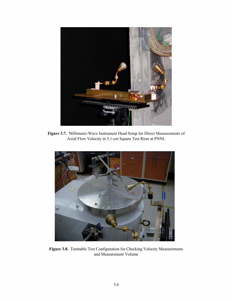
The measurement position in Figure 3.6 is near the wall (‘0 in.’ position in Figure 3.4). The distribution of average velocities at this location is seen to peak at roughly 1 m/s. The transient measurement shows peaks varying over the range of 0.5 to 5 m/s with most often peaks are between 1 and 2 m/s. This looks reasonably consistent with the time average data in Figure 3.4.
Figure 3.3. Velocity Distributions near Center of Riser for Range of Solids Loadings
3.4
Figure 3.4. Velocity Distributions at Four Positions across Riser Cross-Section (‘0 in.’ Is Adjacent to Wall, ‘3 in.’ Is Near Center of 14cm (6 in.) ID Riser)
Figure 3.5. Time Variation of Velocity near Riser Center (1% Loading)
3.5
Figure 3.6. Time Variation of Velocity Adjacent to Wall of Riser (1% Loading)
3.3 Second Generation Prototype
Three significant changes were made in producing the final prototype for installation and measurements in the SNL riser:
1. new antenna configuration to provide direct measurement of axial velocity 2. a mounting system with traverse and a window design that would enable refraction-free
measurements across the riser section 3. a software interface for control of the instrument and for acquiring and processing data
These modifications are described in this section.
The new antenna configuration for direct measurement of axial velocity is shown in Figure 3.7. This required reconfiguring the waveguides that connect the instrument and the antennas.
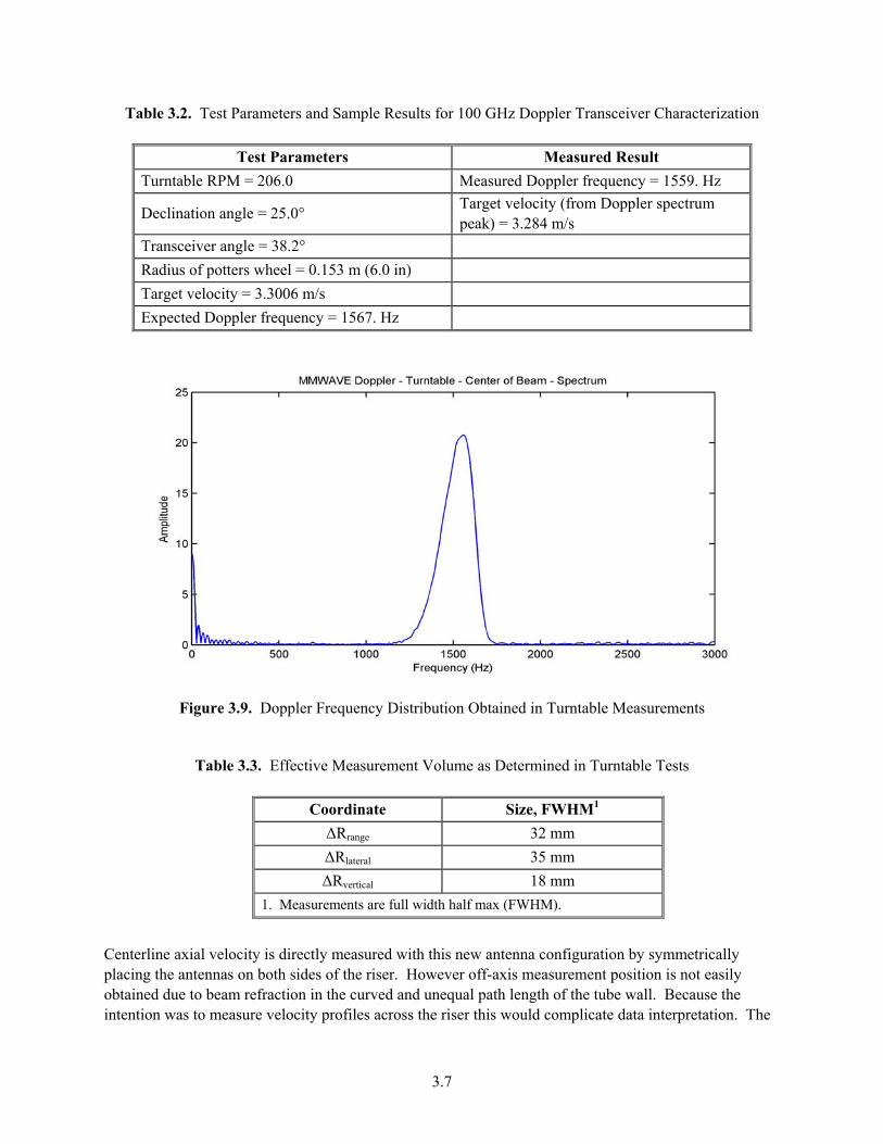
Benchtop testing was completed to establish the effective measurement volume with this antenna configuration and to verify indicated velocities against a known target. This was accomplished by focusing the measurement volume on a single target located at a fixed radius on a “potters wheel” turntable. This configuration is shown in Figure 3.8. Conditions for a sample test and measured results are given in Table 3.2. The Doppler frequency distribution for this test is shown in Figure 3.9. By translating the instrument and measuring signal strength, the effective measurement volume was established. These dimensions are shown in Table 3.3.
3.6
Figure 3.7. Millimeter-Wave Instrument Head Setup for Direct Measurements of Axial Flow Velocity in 5.1-cm Square Test Riser at PNNL
Figure 3.8. Turntable Test Configuration for Checking Velocity Measurements and Measurement Volume
3.7
Table 3.2. Test Parameters and Sample Results for 100 GHz Doppler Transceiver Characterization
Test Parameters Measured Result Turntable RPM = 206.0 Measured Doppler frequency = 1559. Hz
Declination angle = 25.0° Target velocity (from Doppler spectrum peak) = 3.284 m/s
Transceiver angle = 38.2° Radius of potters wheel = 0.153 m (6.0 in) Target velocity = 3.3006 m/s Expected Doppler frequency = 1567. Hz
Figure 3.9. Doppler Frequency Distribution Obtained in Turntable Measurements
Table 3.3. Effective Measurement Volume as Determined in Turntable Tests
Coordinate Size, FWHM1 ΔRrange 32 mm ΔRlateral 35 mm ΔRvertical 18 mm
1. Measurements are full width half max (FWHM).
Centerline axial velocity is directly measured with this new antenna configuration by symmetrically placing the antennas on both sides of the riser. However off-axis measurement position is not easily obtained due to beam refraction in the curved and unequal path length of the tube wall. Because the intention was to measure velocity profiles across the riser this would complicate data interpretation. The
3.8
solution was to manufacture a window section out of low density (thus low refraction), foam material. The foam window replaced a section of acrylic tube removed from a riser pipe segment.
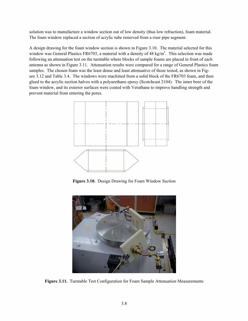
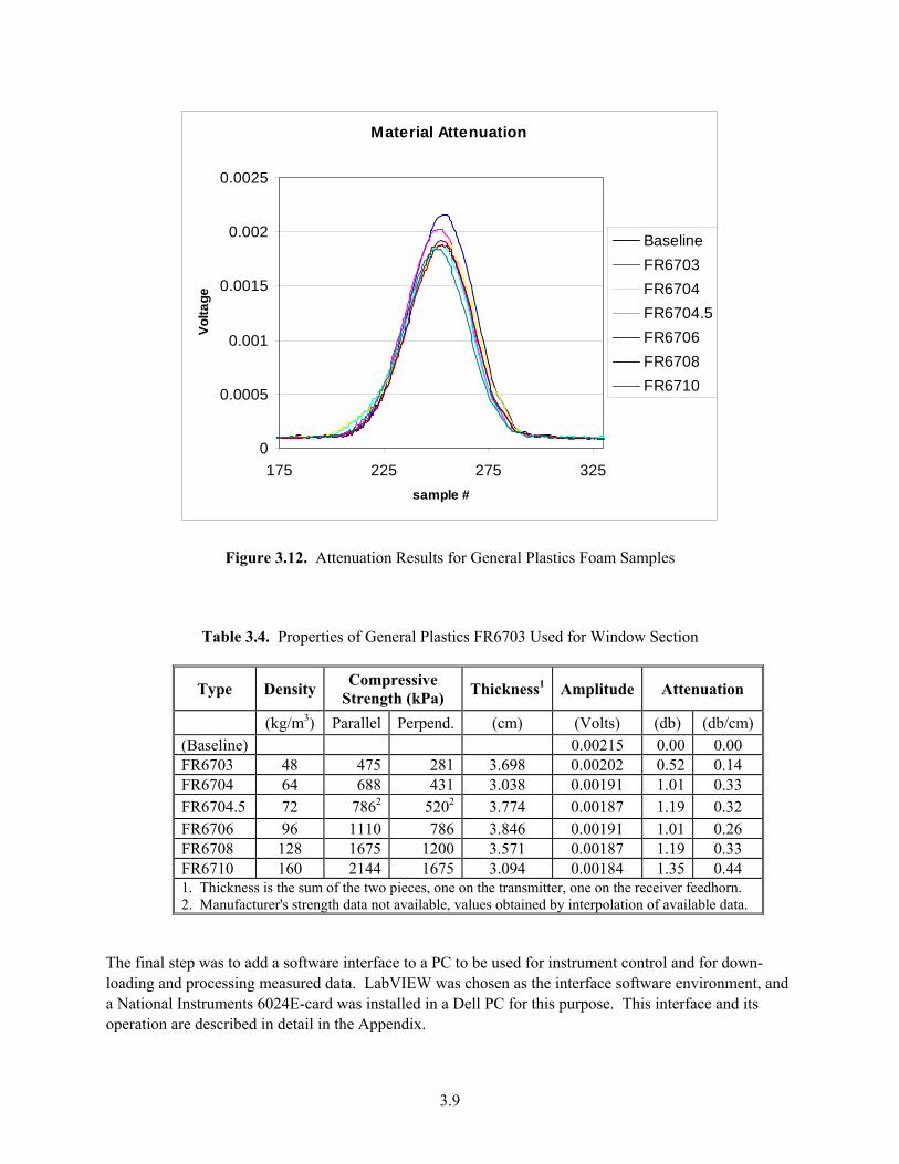
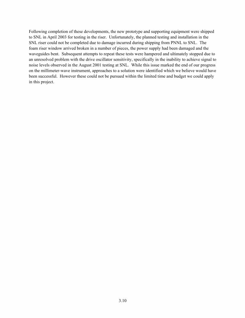
A design drawing for the foam window section is shown in Figure 3.10. The material selected for this window was General Plastics FR6703, a material with a density of 48 kg/m3. This selection was made following an attenuation test on the turntable where blocks of sample foams are placed in front of each antenna as shown in Figure 3.11. Attenuation results were compared for a range of General Plastics foam samples. The chosen foam was the least dense and least attenuative of those tested, as shown in Fig-ure 3.12 and Table 3.4. The windows were machined from a solid block of the FR6703 foam, and then glued to the acrylic section halves with a polyurethane epoxy (Scotchcast 2104). The inner bore of the foam window, and its exterior surfaces were coated with Verathane to improve handling strength and prevent material from entering the pores.
Figure 3.10. Design Drawing for Foam Window Section
Figure 3.11. Turntable Test Configuration for Foam Sample Attenuation Measurements
3.9
Material Attenuation
0
0.0005
0.001
0.0015
0.002
0.0025
175 225 275 325sample #
Volta
ge
BaselineFR6703FR6704FR6704.5FR6706FR6708FR6710
Figure 3.12. Attenuation Results for General Plastics Foam Samples
Table 3.4. Properties of General Plastics FR6703 Used for Window Section
Type Density Compressive Strength (kPa) Thickness1 Amplitude Attenuation
(kg/m3) Parallel Perpend. (cm) (Volts) (db) (db/cm) (Baseline) 0.00215 0.00 0.00 FR6703 48 475 281 3.698 0.00202 0.52 0.14 FR6704 64 688 431 3.038 0.00191 1.01 0.33 FR6704.5 72 7862 5202 3.774 0.00187 1.19 0.32 FR6706 96 1110 786 3.846 0.00191 1.01 0.26 FR6708 128 1675 1200 3.571 0.00187 1.19 0.33 FR6710 160 2144 1675 3.094 0.00184 1.35 0.44 1. Thickness is the sum of the two pieces, one on the transmitter, one on the receiver feedhorn. 2. Manufacturer's strength data not available, values obtained by interpolation of available data.
The final step was to add a software interface to a PC to be used for instrument control and for down-loading and processing measured data. LabVIEW was chosen as the interface software environment, and a National Instruments 6024E-card was installed in a Dell PC for this purpose. This interface and its operation are described in detail in the Appendix.
3.10
Following completion of these developments, the new prototype and supporting equipment were shipped to SNL in April 2003 for testing in the riser. Unfortunately, the planned testing and installation in the SNL riser could not be completed due to damage incurred during shipping from PNNL to SNL. The foam riser window arrived broken in a number of pieces, the power supply had been damaged and the waveguides bent. Subsequent attempts to repeat these tests were hampered and ultimately stopped due to an unresolved problem with the drive oscillator sensitivity, specifically in the inability to achieve signal to noise levels observed in the August 2001 testing at SNL. While this issue marked the end of our progress on the millimeter-wave instrument, approaches to a solution were identified which we believe would have been successful. However these could not be pursued within the limited time and budget we could apply in this project.
4.1
4.0 Ultrasonic Tomography
Desired measurements in the SNL riser include flow velocities and particle concentration. Riser flows of interest have velocities of up to 10 m/s with densely loaded particulate (up to 25% by volume). The ultra-sonic tomography system being developed for this application at PNNL is based on acoustic time of flight (TOF) measurements using air-coupled transducers operating at 125 kHz. In this system, TOF measure-ments from a multi-sensor array will provide velocity distribution through topographic inversion. Signal attenuation will provide the concentration distribution.
At the completion of this project, an operating acoustic tomography system was not yet finished. How-ever considerable development was completed toward that goal and results in prototype testing indicate a high probability of success in applying the technique to similar applications in the future. This section of the report describes progress and remaining work toward this goal.
4.1 Approach
4.1.1 Flow Velocity
Active ultrasonic measurements of gas velocities in gas-solid flows are difficult to make. The suspen-sions are considerably more attenuating than air, and the environment is dominated by passive acoustic noise, leading to very low signal-to-noise ratios. Low frequencies are required to reduce attenuation making Doppler techniques based on scatter from particles impractical. Ultrasonic transducers are relatively limited in the peak signal power they can generate, making it difficult to overcome attenuation and noise.
Robust measurements can be made of the TOF of an ultrasonic pulse in suspensions. The TOF between two points, ‘a’ and ‘b,’ on the periphery of the flow is a function of the speed of sound, c, and the velocity, v, along the path of the beam according to
vacdl
ab
breceiver
artransmitteab •+
= ∫@
@
τ (4.1)
where aab is a unit vector along the path of the beam. This measurement of velocity is not dependent, as are Doppler measurements, upon receiving sound backscattered from particles. A large number of TOF measurements, rapidly made over independent paths, can provide a real time image of the gas velocity field in a pipe or vessel by the application of tomographic reconstruction techniques (Johnson et al. 1977).
4.2 Tomographic Reconstruction
A tomographic reconstruction was used to determine the effect on image quality of measurement noise in the time-of-flight data. By judging the quality of the reconstructed image, specifications could be set on required repeatability of the TOF measurements. The specifications were used in the construction of the ultrasonic front-end.
4.2
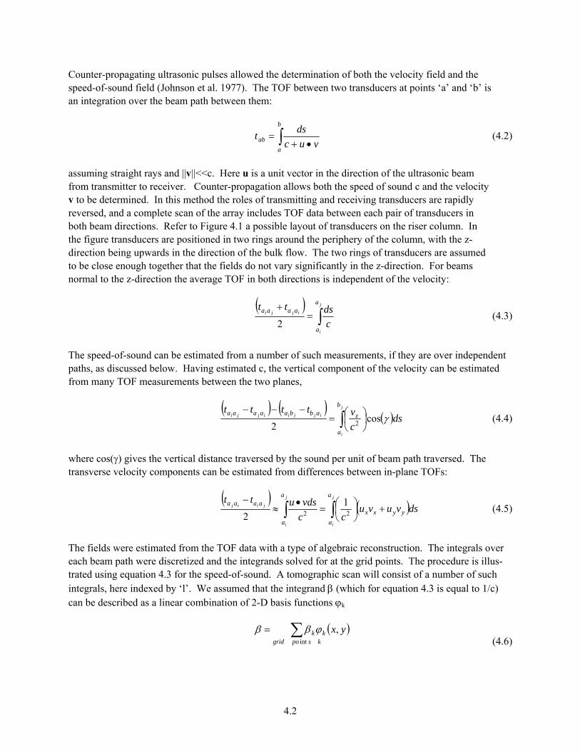
Counter-propagating ultrasonic pulses allowed the determination of both the velocity field and the speed-of-sound field (Johnson et al. 1977). The TOF between two transducers at points ‘a’ and ‘b’ is an integration over the beam path between them:
∫ •+=
b
aab vuc
dst (4.2)
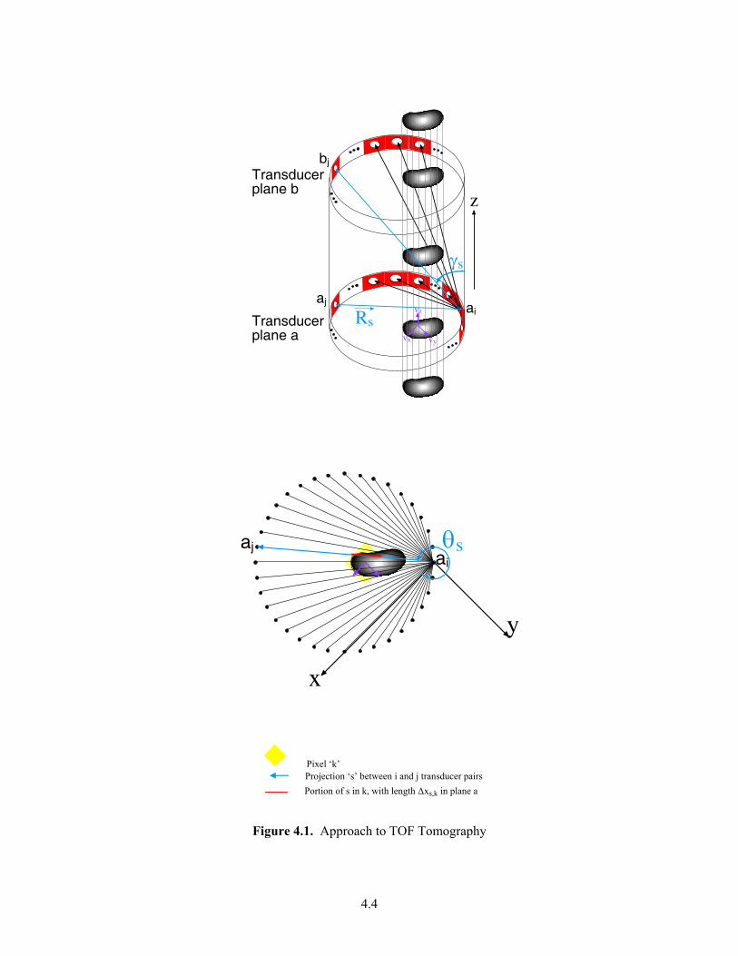
assuming straight rays and ||v||<<c. Here u is a unit vector in the direction of the ultrasonic beam from transmitter to receiver. Counter-propagation allows both the speed of sound c and the velocity v to be determined. In this method the roles of transmitting and receiving transducers are rapidly reversed, and a complete scan of the array includes TOF data between each pair of transducers in both beam directions. Refer to Figure 4.1 a possible layout of transducers on the riser column. In the figure transducers are positioned in two rings around the periphery of the column, with the z-direction being upwards in the direction of the bulk flow. The two rings of transducers are assumed to be close enough together that the fields do not vary significantly in the z-direction. For beams normal to the z-direction the average TOF in both directions is independent of the velocity:
( )∫=
+ j
i
ijji
a
a
aaaa
cdstt
2 (4.3)
The speed-of-sound can be estimated from a number of such measurements, if they are over independent paths, as discussed below. Having estimated c, the vertical component of the velocity can be estimated from many TOF measurements between the two planes,
( ) ( )( )ds
cvtttt j
i
ijjiijji
b
a
zabbaaaaa γcos2 2∫ ⎟
⎠⎞
⎜⎝⎛=
−−− (4.4)
where cos(γ) gives the vertical distance traversed by the sound per unit of beam path traversed. The transverse velocity components can be estimated from differences between in-plane TOFs:
( ) ( )∫ ∫ +⎟⎠⎞
⎜⎝⎛=
•≈
− j
i
j
i
jiij
a
a
a
ayyxx
aaaa dsvuvucc
vdsutt22
12
(4.5)
The fields were estimated from the TOF data with a type of algebraic reconstruction. The integrals over each beam path were discretized and the integrands solved for at the grid points. The procedure is illus-trated using equation 4.3 for the speed-of-sound. A tomographic scan will consist of a number of such integrals, here indexed by ‘l’. We assumed that the integrand β (which for equation 4.3 is equal to 1/c) can be described as a linear combination of 2-D basis functions ϕk
( )∑=kspogrid
kk yxint
,ϕββ (4.6)
4.3
where the sum is over all grid points in the cross-section of the riser. It is presumed that the basis func-tions are localized, with one function per grid point (the functions do overlap each other), the values of the basis functions summing to unity at each grid point. In this work the basis functions used were bi-linear splines. Each integral is then a linear combination of integrals over the basis functions. For the lth ray between transducers ai and aj:
( )( ) ( )( ) ∑∫ ∑ ∫ =≈=
+≡
klkkl
a
a k ofdomainllkkl
aaaal xdssysxds
tty
j
i k
ijji βϕββϕ
,2
(4.7)
There were similar discretizations for equations 4.4 and 4.5. The coefficients βk were estimated by linear regression. They were found by solving modified normal equations,
( ) yXHXX TT •=•+• βλ (4.8)
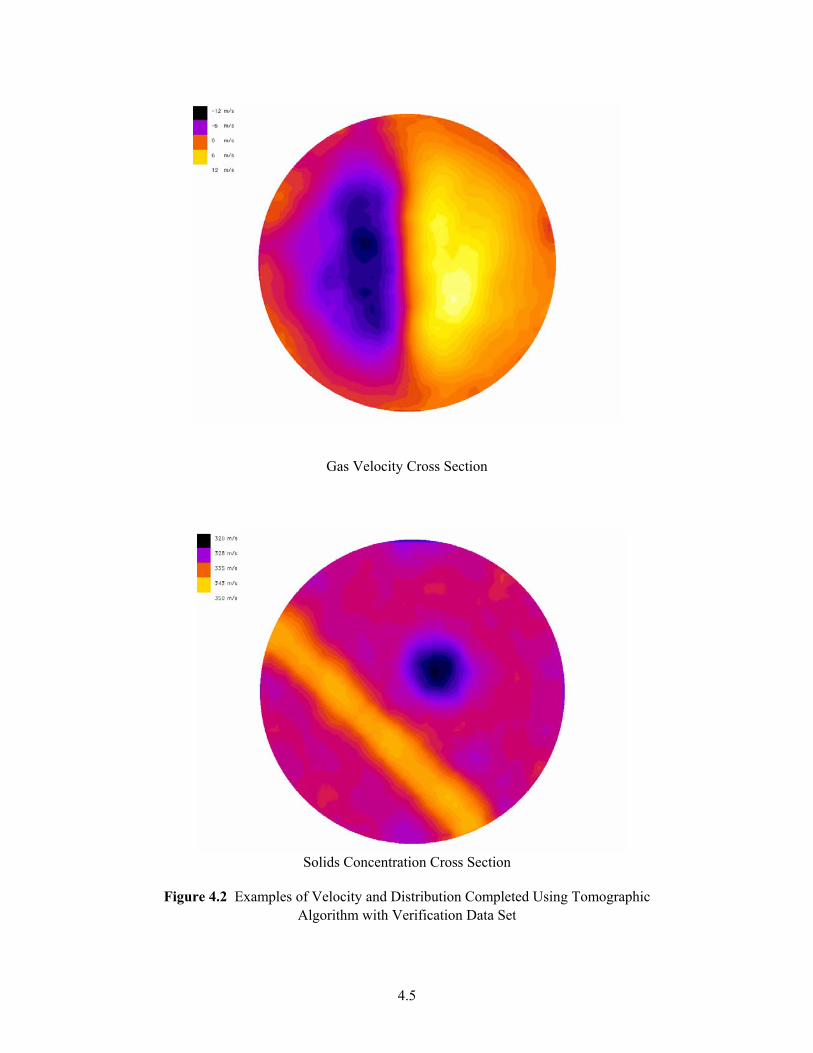
where y is a vector of the average of forward and backward TOFs of length equal to the number of beam paths in the scan. β is a vector of length equal to the number of grid points formed from the coefficients βk. X is a matrix of the path integrals of the basis functions. The matrix X was quite sparse, as most beam paths cross the domains of only a small fraction of the basis functions. Linear regularization (Press et al. 1992) was used to reduce the noise in the solution. For this, matrix H was chosen to dampen the system by averaging over neighboring grid points and coefficient λ set to given the desired degree of dampening. Example reconstructions from simulated TOF data are shown in Figure 4.2. The simulated TOF data were constructed from assumed velocity and speed-of-sound distributions and then various ranges of measurement noise were added. The velocity and speed-of-sound distributions were not intended to be physically realistic, merely values to test the reconstruction algorithm. Pictured in the left half of the figure is a reconstruction of axial velocities, the flow being upwards in the right half of the riser, downwards on the left half. Pictured on the right half of the figure is a reconstruction from sound speeds of the solids loading. The presumed solids distribution had a block and a stripe pattern. From such reconstructions it was estimated that TOF values measured to within ± 2 to 4 μs would give acceptable images of axial velocity. TOF accuracy would need to improve to ± 1 μs to give acceptable images of the transverse velocities. 4.3 Time-of-Flight Measurement
A TOF measurement system must have four key characteristics to be the basis of an accurate, highly time- and spatially resolved tomographic system:
1. Adequate signal-to-noise ratio to enable the detection of a pulse that has traversed an attenuating fluid in a noisy environment.
2. Accurate measurement of the TOF of each pulse. 3. An ability to discriminate, after reception, pulses that have arrived from multiple sources. 4. An ability to rapidly swap transmitter and receiver pairs to gather data from reversed
“counter-propagating beams.”
4.4
Figure 4.1. Approach to TOF Tomography
Pixel ‘k’ Projection ‘s’ between i and j transducer pairs
Portion of s in k, with length Δxs,k in plane a
vx vy
vz
γs
z
Transducer plane b
Transducer plane a
aiaj
bj
Rs
x
y
θsajai
4.5
Gas Velocity Cross Section
Solids Concentration Cross Section
Figure 4.2 Examples of Velocity and Distribution Completed Using Tomographic Algorithm with Verification Data Set
4.6
The TOF measurement system described in this report was designed to excel in each of these key areas. Very long pulses were used to increase pulse energy, and therefore signal-to-noise ratio, in attenuating media and noisy environments. The TOF of pulses was determined by cross-correlating the transmitted signal with the received waveforms. This had the effect of compressing the long, low-amplitude pulse into a narrow, tall peak rising above baseline noise (Lam et al. 1976). The height of the peak was pro-portional to the length of the pulse. Both the width of the peak in the cross correlation and the time resolution of the resulting TOF were inversely proportional to the bandwidth of the ultrasonic pulse. The bandwidth was increased by phase-shift modulating the drive signal. The modulation had the effect of giving the pulse a signature. The width of the peak in the correlation function was inversely proportional to the bandwidth of the modulated pulse. The polyphase modulations used were spectrum-spreading code sequences developed for cell phone use (Lötter et al. 1994). Unique code sequences (with minimal cross correlation) were assigned to each transmitter, allowing simultaneous transmissions to be distinguished at the receiver. The modulation signatures were also quite distinct from the white noise-like passive acous-tic noise present in the riser column. This distinction allowed the pulses to be heard by the receiver in the presence of noise. Finally a new electronic system was designed for multiple high-speed measurements of TOF in gas-solid flows. The system comprised an array of transceiver units operating under computer control, making possible arbitrary pulse sequencing and arbitrary waveform generation from each trans-mitter. With this system, transducers can be rapidly switched from transmission to reception mode. The system was designed to serve as the front end for a high-speed tomographic imaging system.
In this work, 2.35-ms pulses of 125-kHz ultrasound were modulated by sequences of phase shifts φ(t). A complex representation of the transmitted baseband signal is
( ) ( ) ( )[ ] ( )[ ]}sin{cos tittptm φφ += (4.9)
where p(t) denotes the on-off pulse modulation of the continuous 125-kHz carrier waveform. The received signal was quadrature demodulated and has a complex representation of
( ) iQItS += (4.10)
which, neglecting filtering by the transducers and the medium, is approximately a time- and phase-shifted copy of the transmitted signal:
( ) ( ) noisettmetS oti oc +−≈ − ωα (4.11)
In this equation, to is the TOF of the pulse, ωc is the carrier frequency, and α is an attenuation factor. The exponential factor is a phase shift resulting from demodulation. The TOF can be found from the location of the maximum in a plot versus time of the modulus of the cross-correlation of the transmitted signal with the received signal |S m*|2. The received waveforms were post-processed to obtain the TOF values.
4.3.1 Multi-AUP Prototype
Early in this project, testing of acoustic TOF concepts was done using PNNL’s AUP. This system supported only a single transducer pair and these early tests showed that significant modifications would be required to deliver the sensitivity and resolution required for tomography. The multi-AUP is the new system of front-end electronics that was constructed to meet this need for the large number of transducer pairs required in a tomographic system. More specifically, the multi-AUP is a fully self-contained system
4.7
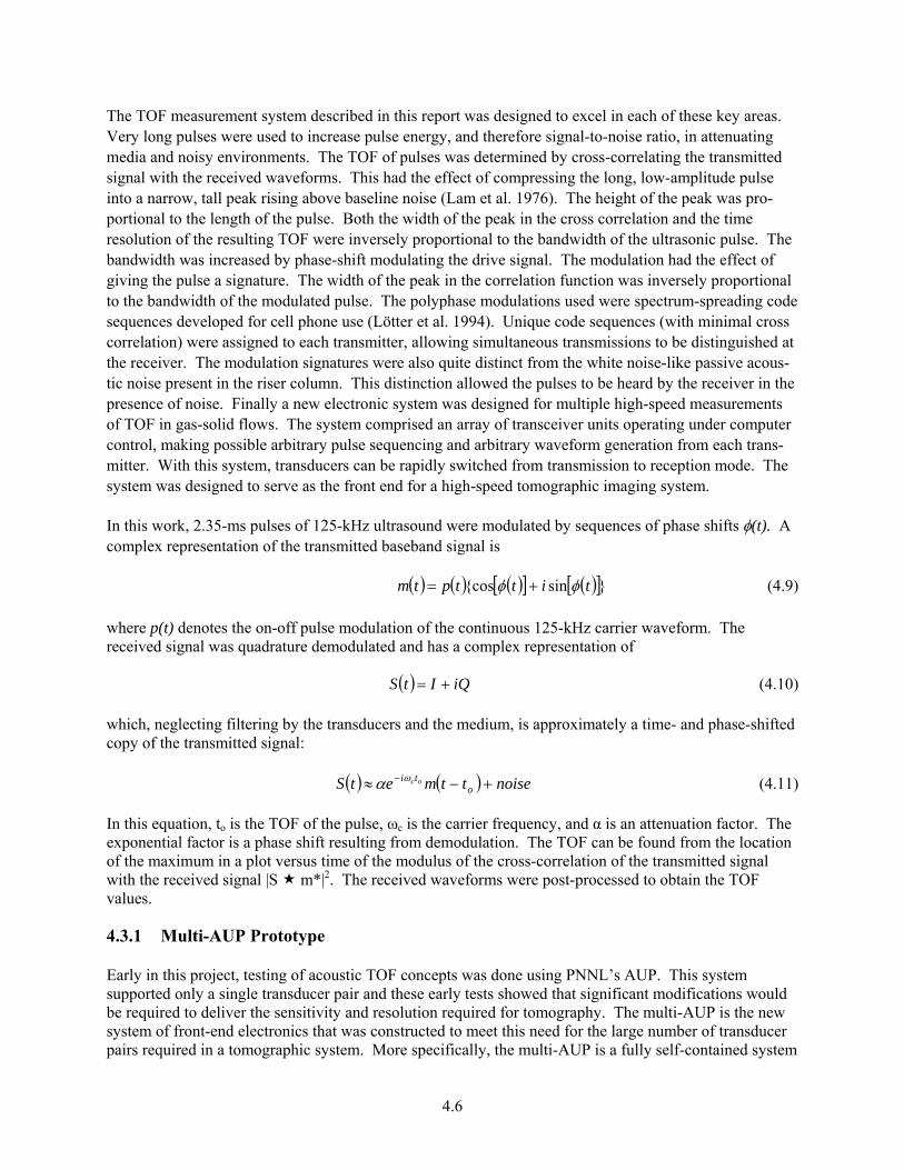
to synthesize, sequence, and amplify waveforms to drive the ultrasonic transducers, demodulate and digitize the received waveforms, and download the received waveforms to a PC for later post-processing. Figure 4.3 is a simplified schematic of the system.
The electronics consist of a series of transceiver boards mounted in a rack containing an embedded controller with a PC-based configuration and data acquisition system. These components are shown in Figures 4.4, 4.5, and 4.6. Each transceiver board is divided into transmitter and receiver sections. The transmitter section includes an arbitrary waveform generator and radio frequency (RF) power amplifier. The receiver section consists of a quadrature receiver and an analog-to-digital converter that discretizes received waveforms for storage on the PC. The design and operation of the system are discussed below.
Figure 4.3. System Specifications and Detail of a Single Transceiver Board
4.3.1.1 Embedded Controller
The embedded controller sits on the backplane of the electronics rack and is common to all transceivers installed. A controller can operate up to 32 transceivers driving 32 transducers in an array for tomography applications. Controllers and racks can be ganged to allow construction of even larger arrays.
4.8
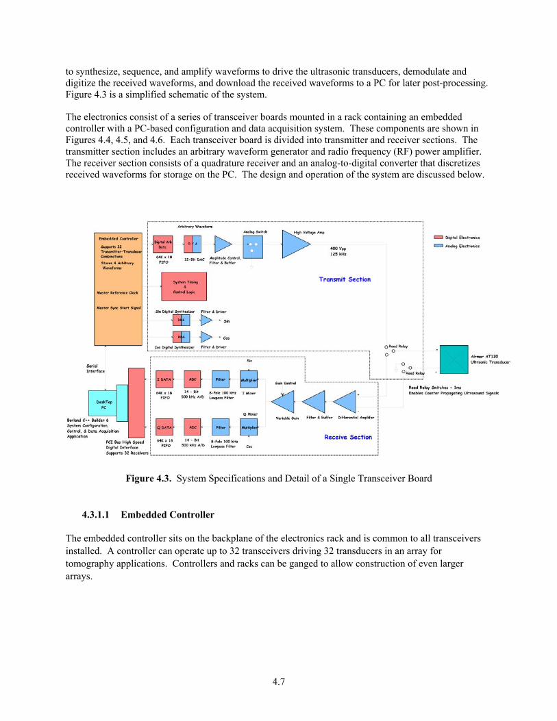
Figure 4.4. Transceiver Board – One per Transducer
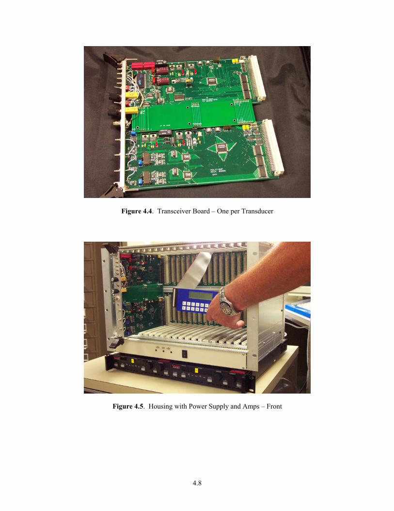
Figure 4.5. Housing with Power Supply and Amps – Front
4.9
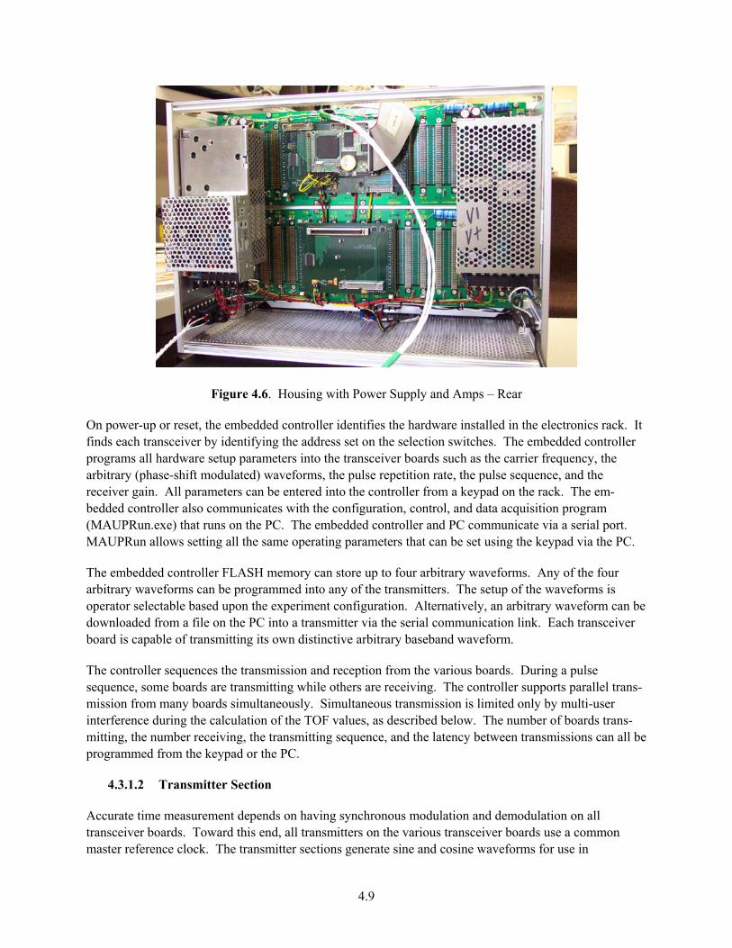
Figure 4.6. Housing with Power Supply and Amps – Rear
On power-up or reset, the embedded controller identifies the hardware installed in the electronics rack. It finds each transceiver by identifying the address set on the selection switches. The embedded controller programs all hardware setup parameters into the transceiver boards such as the carrier frequency, the arbitrary (phase-shift modulated) waveforms, the pulse repetition rate, the pulse sequence, and the receiver gain. All parameters can be entered into the controller from a keypad on the rack. The em-bedded controller also communicates with the configuration, control, and data acquisition program (MAUPRun.exe) that runs on the PC. The embedded controller and PC communicate via a serial port. MAUPRun allows setting all the same operating parameters that can be set using the keypad via the PC.
The embedded controller FLASH memory can store up to four arbitrary waveforms. Any of the four arbitrary waveforms can be programmed into any of the transmitters. The setup of the waveforms is operator selectable based upon the experiment configuration. Alternatively, an arbitrary waveform can be downloaded from a file on the PC into a transmitter via the serial communication link. Each transceiver board is capable of transmitting its own distinctive arbitrary baseband waveform.
The controller sequences the transmission and reception from the various boards. During a pulse sequence, some boards are transmitting while others are receiving. The controller supports parallel trans-mission from many boards simultaneously. Simultaneous transmission is limited only by multi-user interference during the calculation of the TOF values, as described below. The number of boards trans-mitting, the number receiving, the transmitting sequence, and the latency between transmissions can all be programmed from the keypad or the PC.
4.3.1.2 Transmitter Section
Accurate time measurement depends on having synchronous modulation and demodulation on all transceiver boards. Toward this end, all transmitters on the various transceiver boards use a common master reference clock. The transmitter sections generate sine and cosine waveforms for use in
4.10
demodulation. These waveforms are generated using direct digital synthesizers and are locked in phase on all boards. One master start pulse is used by all the transmitters to start sending the arbitrary wave-forms; thus, all transmitted signals have a common time reference. The start pulse begins at a zero crossing of the sine waveform used for demodulation.
Each arbitrary waveform is a 125-kHz sinusoidal waveform that has a sequence of discrete phase shifts encoded into the signal. The polyphase modulation used on each board was one of the seven unique 49-long code sequences described in reference (Lötter et al. 1994). In this work, each element of a code sequence was six cycles of the 125-kHz carrier long (code elements shorter than four cycles were found to be ineffective). The digital version of an arbitrary waveform is stored in a first-in-first-out (FIFO) buffer on a transceiver. The 12-bit digital data are clocked out and converted to analog. The analog signal is filtered and amplified and can be set to a maximum of 400 volts peak-to-peak to drive an ultra-sonic transducer (Airmar model AT120). A set of fast switching (switch plus bounce times less than 1ms) reed relays on a board are used to change between transmit and receive modes of operation.
4.3.1.3 Receiver Section
The receivers use a differential input instrumentation amplifier as the initial amplification of the receive signal from the transducer. After additional amplification and filtering, the receive signal is split into I and Q signal paths. Each I and Q are demodulated using a mixer-multiplier and then filtered using an eight-pole, 100-kHz low-pass filter. Each I and Q are then digitized at 500 kHz with 14 bits of resolution. The I and Q digital data are stored in separate FIFOs for later retrieval by the PC. The PC reads I and Q data via a PCI bus high-speed digital interface board.
4.3.1.4 Configuration, Control, and Data Acquisition System
A PC with a PCI bus high speed digital interface board implements the data acquisition system. Borland C++ Builder 6 was used to develop the MAUPRun program used to configure the system hardware, control system operations, and acquire I and Q data. The baseband I and Q data received after each pulse firing sequence are saved to a file for subsequent processing to obtain the TOF values.
4.3.1.5 Operations
Setting up a test involves defining when a transducer will be a transmitter and when it will be a receiver. The repetition rate sets the basic rate at which the system is pulsed. During each repetition period, two transducer configurations are defined in terms of which transducer is a transmitter and which a receiver. The switching time between the two configurations is 1 ms. For example, transducer “a” can transmit its arbitrary ultrasonic waveform through the test material to receiving transducer “b” then 1 ms later the transducers can reverse roles and “b” transmit to receiver “a.” The ability to rapidly reverse transits of ultrasound along the same beam path supports tomographic applications. Once the sequences are configured and the system started, it repeats at the repetition rate until stopped.
4.3.2 Multi-AUP Prototype Testing
TOF was determined by cross-correlating the demodulated received waveforms with the transmitted code sequence as discussed above. These times are the sums of the true TOF plus a constant delay time intro-duced by the transducer and the electronics. The TOF of echoes taken in an empty riser section were used
4.11
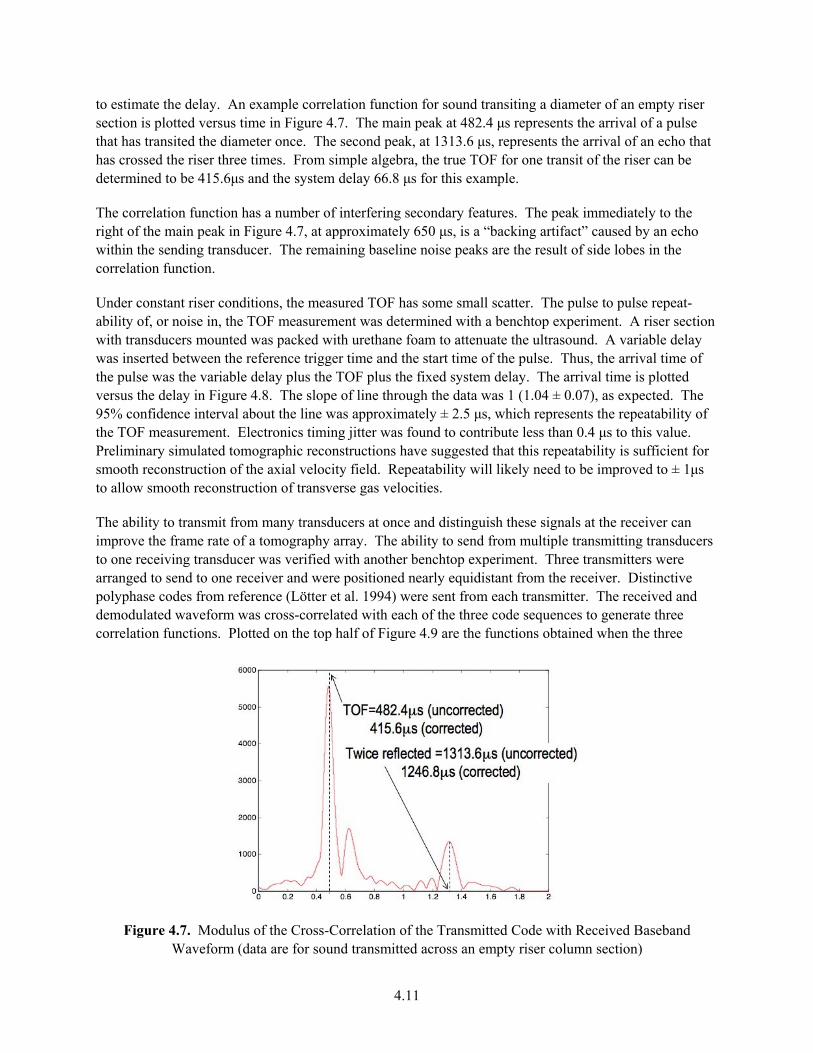
to estimate the delay. An example correlation function for sound transiting a diameter of an empty riser section is plotted versus time in Figure 4.7. The main peak at 482.4 μs represents the arrival of a pulse that has transited the diameter once. The second peak, at 1313.6 μs, represents the arrival of an echo that has crossed the riser three times. From simple algebra, the true TOF for one transit of the riser can be determined to be 415.6μs and the system delay 66.8 μs for this example.
The correlation function has a number of interfering secondary features. The peak immediately to the right of the main peak in Figure 4.7, at approximately 650 μs, is a “backing artifact” caused by an echo within the sending transducer. The remaining baseline noise peaks are the result of side lobes in the correlation function.
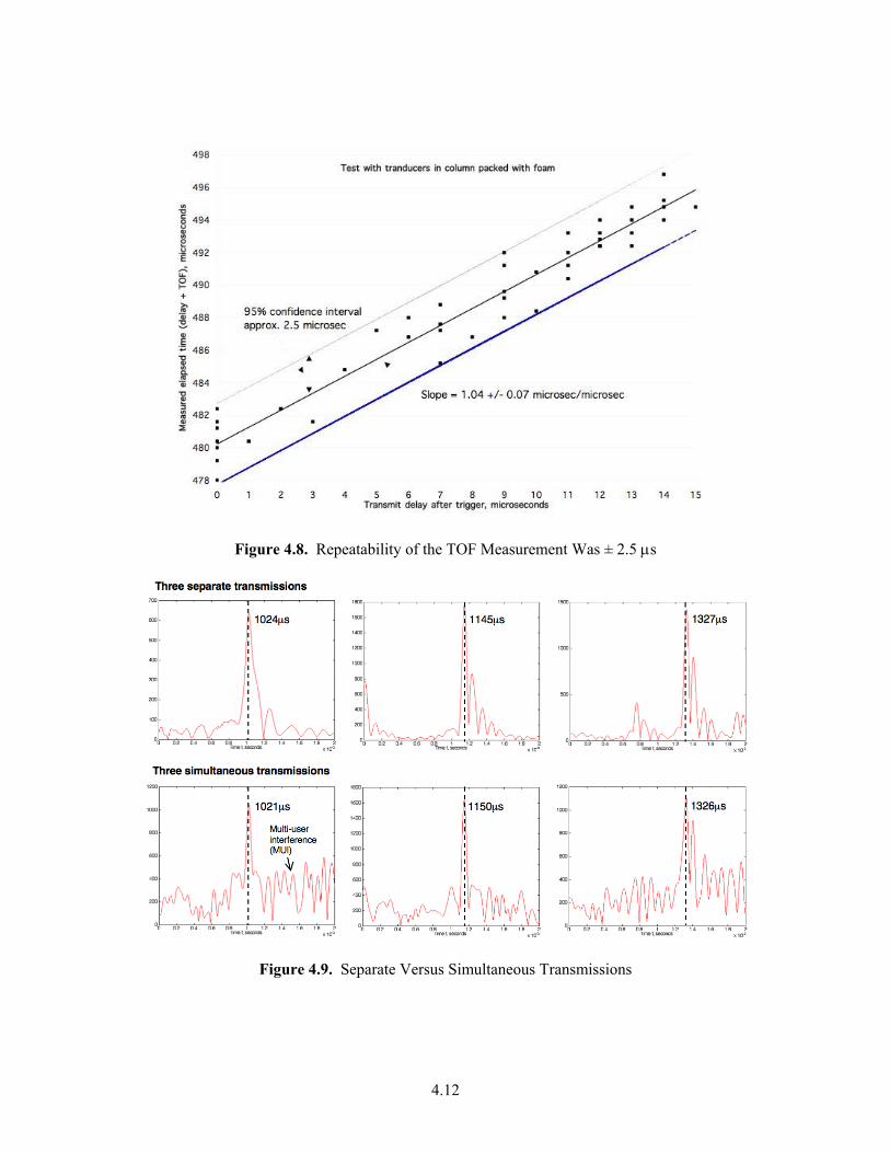
Under constant riser conditions, the measured TOF has some small scatter. The pulse to pulse repeat-ability of, or noise in, the TOF measurement was determined with a benchtop experiment. A riser section with transducers mounted was packed with urethane foam to attenuate the ultrasound. A variable delay was inserted between the reference trigger time and the start time of the pulse. Thus, the arrival time of the pulse was the variable delay plus the TOF plus the fixed system delay. The arrival time is plotted versus the delay in Figure 4.8. The slope of line through the data was 1 (1.04 ± 0.07), as expected. The 95% confidence interval about the line was approximately ± 2.5 μs, which represents the repeatability of the TOF measurement. Electronics timing jitter was found to contribute less than 0.4 μs to this value. Preliminary simulated tomographic reconstructions have suggested that this repeatability is sufficient for smooth reconstruction of the axial velocity field. Repeatability will likely need to be improved to ± 1μs to allow smooth reconstruction of transverse gas velocities.
The ability to transmit from many transducers at once and distinguish these signals at the receiver can improve the frame rate of a tomography array. The ability to send from multiple transmitting transducers to one receiving transducer was verified with another benchtop experiment. Three transmitters were arranged to send to one receiver and were positioned nearly equidistant from the receiver. Distinctive polyphase codes from reference (Lötter et al. 1994) were sent from each transmitter. The received and demodulated waveform was cross-correlated with each of the three code sequences to generate three correlation functions. Plotted on the top half of Figure 4.9 are the functions obtained when the three
Figure 4.7. Modulus of the Cross-Correlation of the Transmitted Code with Received Baseband Waveform (data are for sound transmitted across an empty riser column section)
4.12
Figure 4.8. Repeatability of the TOF Measurement Was ± 2.5 μs
Figure 4.9. Separate Versus Simultaneous Transmissions
4.13
transmissions did not overlap in time, yielding arrival times of 1024, 1145, and 1327 μs. Plotted on the bottom half of the figure the functions obtained when the three transmissions were done simultaneously, yielding arrival times of 1021, 1150, and 1326 μs. These times are equivalent, within the repeatability of the experiment, to those obtained with separate transmissions. The functions obtained with simultaneous transmission do show some increased baseline noise attributed to non-zero cross-correlations between the three transmitted codes (multi-user interference).
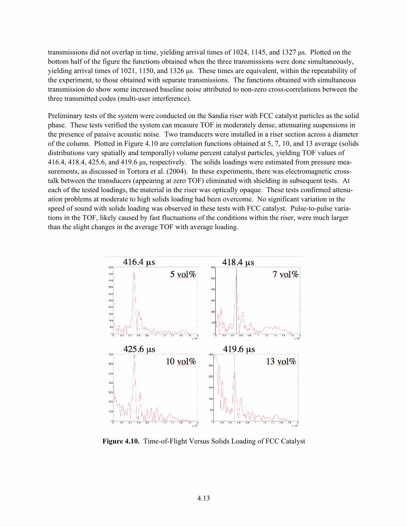
Preliminary tests of the system were conducted on the Sandia riser with FCC catalyst particles as the solid phase. These tests verified the system can measure TOF in moderately dense, attenuating suspensions in the presence of passive acoustic noise. Two transducers were installed in a riser section across a diameter of the column. Plotted in Figure 4.10 are correlation functions obtained at 5, 7, 10, and 13 average (solids distributions vary spatially and temporally) volume percent catalyst particles, yielding TOF values of 416.4, 418.4, 425.6, and 419.6 μs, respectively. The solids loadings were estimated from pressure mea-surements, as discussed in Tortora et al. (2004). In these experiments, there was electromagnetic cross-talk between the transducers (appearing at zero TOF) eliminated with shielding in subsequent tests. At each of the tested loadings, the material in the riser was optically opaque. These tests confirmed attenu-ation problems at moderate to high solids loading had been overcome. No significant variation in the speed of sound with solids loading was observed in these tests with FCC catalyst. Pulse-to-pulse varia-tions in the TOF, likely caused by fast fluctuations of the conditions within the riser, were much larger than the slight changes in the average TOF with average loading.
Figure 4.10. Time-of-Flight Versus Solids Loading of FCC Catalyst
4.14
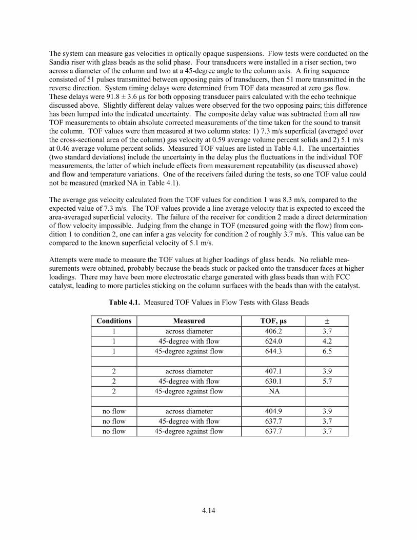
The system can measure gas velocities in optically opaque suspensions. Flow tests were conducted on the Sandia riser with glass beads as the solid phase. Four transducers were installed in a riser section, two across a diameter of the column and two at a 45-degree angle to the column axis. A firing sequence consisted of 51 pulses transmitted between opposing pairs of transducers, then 51 more transmitted in the reverse direction. System timing delays were determined from TOF data measured at zero gas flow. These delays were 91.8 ± 3.6 μs for both opposing transducer pairs calculated with the echo technique discussed above. Slightly different delay values were observed for the two opposing pairs; this difference has been lumped into the indicated uncertainty. The composite delay value was subtracted from all raw TOF measurements to obtain absolute corrected measurements of the time taken for the sound to transit the column. TOF values were then measured at two column states: 1) 7.3 m/s superficial (averaged over the cross-sectional area of the column) gas velocity at 0.59 average volume percent solids and 2) 5.1 m/s at 0.46 average volume percent solids. Measured TOF values are listed in Table 4.1. The uncertainties (two standard deviations) include the uncertainty in the delay plus the fluctuations in the individual TOF measurements, the latter of which include effects from measurement repeatability (as discussed above) and flow and temperature variations. One of the receivers failed during the tests, so one TOF value could not be measured (marked NA in Table 4.1).
The average gas velocity calculated from the TOF values for condition 1 was 8.3 m/s, compared to the expected value of 7.3 m/s. The TOF values provide a line average velocity that is expected to exceed the area-averaged superficial velocity. The failure of the receiver for condition 2 made a direct determination of flow velocity impossible. Judging from the change in TOF (measured going with the flow) from con-dition 1 to condition 2, one can infer a gas velocity for condition 2 of roughly 3.7 m/s. This value can be compared to the known superficial velocity of 5.1 m/s.
Attempts were made to measure the TOF values at higher loadings of glass beads. No reliable mea-surements were obtained, probably because the beads stuck or packed onto the transducer faces at higher loadings. There may have been more electrostatic charge generated with glass beads than with FCC catalyst, leading to more particles sticking on the column surfaces with the beads than with the catalyst.
Table 4.1. Measured TOF Values in Flow Tests with Glass Beads
Conditions Measured TOF, μs ± 1 across diameter 406.2 3.7 1 45-degree with flow 624.0 4.2 1 45-degree against flow 644.3 6.5
2 across diameter 407.1 3.9 2 45-degree with flow 630.1 5.7 2 45-degree against flow NA
no flow across diameter 404.9 3.9 no flow 45-degree with flow 637.7 3.7 no flow 45-degree against flow 637.7 3.7
4.15
4.4 Transducer Development
Transducers are our remaining challenge. While our modified commercial transducers will allow us to check out the system and perform the coarse array test, a development effort still remains to give the optimal transducer for a tomographic system. Asking simultaneously for high output, wide bandwidth and wide beam angle is asking a lot. For example, the high bandwidth transducers we had custom made in FY02 suffered considerable loss in output power in the exchange. We are not likely to get all three in any one design, but tradeoffs should be possible (e.g. high resolution, low concentration or low resolu-tion, high concentration). We at PNNL will be looking for ways to fund this remaining development task.
• Tradeoffs in size and penetration with frequency in commercial off the shelf (COTS) transducers • New transducer development – attempts, failures, and ultimately deferral.
5.1
5.0 Conclusions and Recommendations
5.1 Conclusions
During the course of this project, millimeter wave velocimetry was demonstrated in the SNL riser as being capable of making local measurements of solid phase velocities. These measurements were made through the acrylic riser wall and included a range of particle concentrations from 0.1 to 5%. The measurement signal is a spectrum of Doppler shifted frequencies, where the peak magnitude indicates bulk velocity magnitude. Measurements at concentrations up to 20% were attempted, but the bulk axial velocity was not distinguishable from the measurement. Potential exists for measuring turbulence quantities within the sampling volume, but this requires further work to characterize and extract this information from the measured spectrum. Finally, while our measurements focused on axial particle velocity, other velocity components can be resolved by reorienting antennas and simultaneous measurement of three components could be done with replicated instruments.
We have developed an electronics platform and signal-processing scheme that can measure ultrasonic TOF values in light to moderately loaded gas-solid flows. The system is capable of high-speed measure-ments from multiple transducers for tomography applications. We have verified the required timing accuracy and parallel transmission capability in a laboratory environment and demonstrated TOF mea-surement in moderately loaded suspensions of FCC catalyst particles. However, tomography requires fan beam transducers. A measurement of transverse gas velocities requires more repeatable TOF measure-ments, which likely requires greater transducer bandwidth. These requirements are difficult to satisfy as increasing spatial beam width and/or increasing frequency bandwidth greatly reduces the efficiency of the transducer. Transducer installation remains difficult as well. Efficiency in penetrating these suspensions requires direct contact of the transducers with the medium.
5.2 Recommendations
The next step for the millimeter wave velocimetry system should be to determine the cause of the lack of sensitivity in the second generation prototype, make repairs and follow with test of alternate antennae configurations. Following duplication of successful tests and further characterization with this system, use duplicate systems to demonstrate multiple-component velocity measurements. Explore alternate arrangements that provide time resolution for turbulence measurements. Perform further characterization of the measured frequency spectrum, its dependency on bulk particulate loading and velocity distribution. Results of such an investigation will validate bulk velocity measurements and should clarify additional capabilities of the instrument for quantifying velocity distribution and solid-phase turbulence intensity.
The recommended next steps for the ultrasonic tomography system development are to, first, test and develop wide angle, high bandwidth transducers and determine their range of applicability in a prototype system. Then replicate the transducer array and complete the demonstration of acoustic tomography; and finally, explore loadings and range of applicability of the completed system.
6.1
6.0 References
Bhusarapu S, MH Al-Dahhan, MP Dudukovic, SM Trujillo, and TJ O'Hern. 2005. “Experimental Study of the Solids Velocity Field in Gas-Solid Risers.” Ind. Eng. Chem. Res., 44:9739-9749.
Johnson SA, JF Greenleaf, M Tanaka, and G Flandro. 1977. “Reconstructing 3-Dimensional Temperature and Fluid Velocity Vector Fields from Acoustic Transmission Measurements.” ISA Transactions, 16(3):3-15.
Lam F and J Szilard. 1976. “Pulse Compression Techniques in Ultrasonic Non-Destructive Testing.” Ultrasonics, 14:111-114.
Lötter MP and LP Linde. 1994. “A Comparison of Three Families of Spreading Sequences for CDMA Applications.” Communications and Signal Processing. COMSIG-94, Proceedings of the 1994 IEEE South African Symposium, pp. 68-75.
Pfund DM, JA Fort, GP Morgen, and SM Trujillo. April 2006. “Measurement of Gas Velocities in Gas/Solids Flows Using Time-of-Flight Ultrasound.” Proceedings of AIChE 2006 Spring National Meeting, Orlando, Florida.
Press WH, SA Teukolsky, WT Vetterling, and BP Flannery. 1992. “Numerical Recipes in C,” 2nd Edition. Cambridge University Press, United Kingdom.
Tortora PR, SL Ceccio, SM Trujillo, TJ O'Hern, and KA Shollenberger. 2004. “Capacitance Measurements of Solid Concentration in Gas-Solid Flows.” Powder Technology, 148:92-101.
Appendix
Description of Software Interface to Millimeter-Wave Instrument
A.1
Operation Guide for the Millimeter-Wave Doppler Velocity Program
A.2
Index: Overview/Flowchart 3 Recommended Hardware/Software configuration 4 Getting Input Signal 5 Screen shot 6 Running the program 8 Saving output files 9
A.3
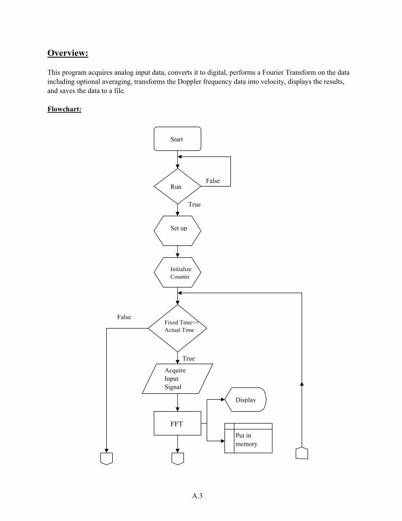
Overview: This program acquires analog input data, converts it to digital, performs a Fourier Transform on the data including optional averaging, transforms the Doppler frequency data into velocity, displays the results, and saves the data to a file. Flowchart:
Start
Run
Set up
Initialize Counter
Fixed Time<= Actual Time
Acquire Input Signal
Put in memory
FFT
False
True
False
True
Display
A.4
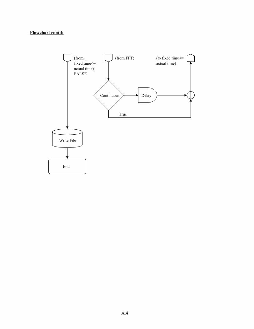
Flowchart contd:
End
Write File
Continuous Delay
True
(from FFT)(from fixed time<= actual time) FALSE
(to fixed time<= actual time)
A.5
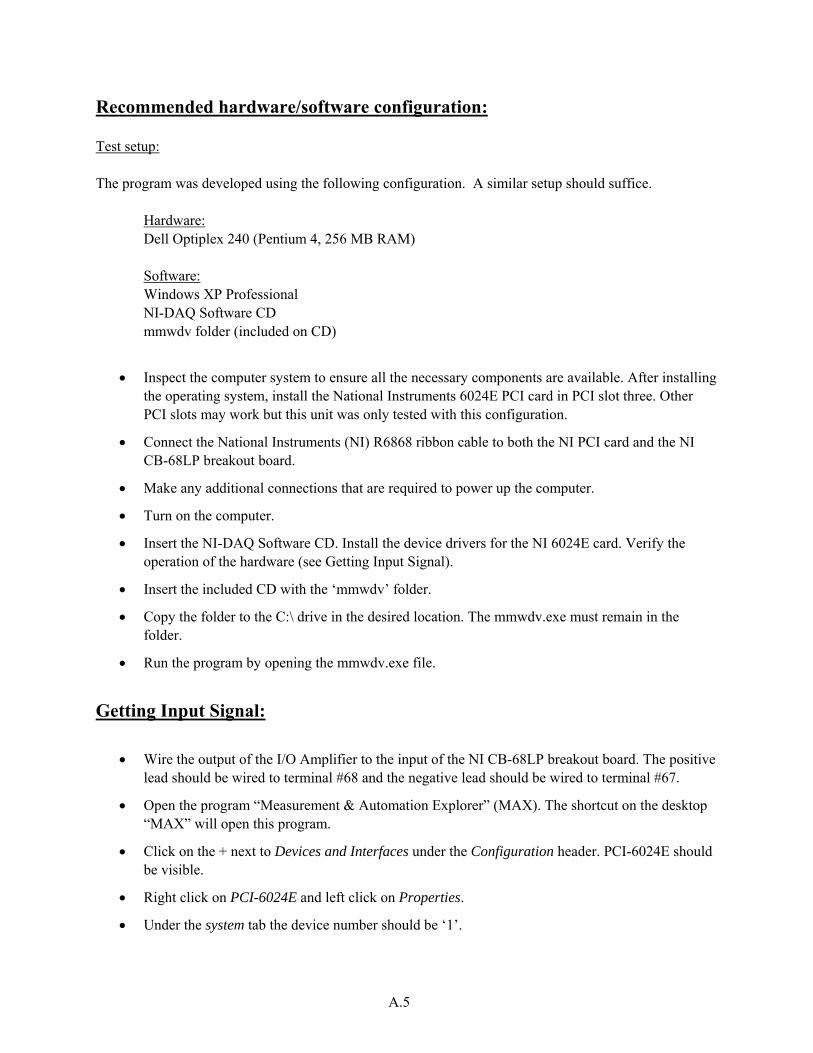
Recommended hardware/software configuration: Test setup: The program was developed using the following configuration. A similar setup should suffice.
Hardware: Dell Optiplex 240 (Pentium 4, 256 MB RAM)
Software: Windows XP Professional NI-DAQ Software CD mmwdv folder (included on CD)
• Inspect the computer system to ensure all the necessary components are available. After installing the operating system, install the National Instruments 6024E PCI card in PCI slot three. Other PCI slots may work but this unit was only tested with this configuration.
• Connect the National Instruments (NI) R6868 ribbon cable to both the NI PCI card and the NI CB-68LP breakout board.
• Make any additional connections that are required to power up the computer.
• Turn on the computer.
• Insert the NI-DAQ Software CD. Install the device drivers for the NI 6024E card. Verify the operation of the hardware (see Getting Input Signal).
• Insert the included CD with the ‘mmwdv’ folder.
• Copy the folder to the C:\ drive in the desired location. The mmwdv.exe must remain in the folder.
• Run the program by opening the mmwdv.exe file.
Getting Input Signal:
• Wire the output of the I/O Amplifier to the input of the NI CB-68LP breakout board. The positive lead should be wired to terminal #68 and the negative lead should be wired to terminal #67.
• Open the program “Measurement & Automation Explorer” (MAX). The shortcut on the desktop “MAX” will open this program.
• Click on the + next to Devices and Interfaces under the Configuration header. PCI-6024E should be visible.
• Right click on PCI-6024E and left click on Properties.
• Under the system tab the device number should be ‘1’.
A.6
• Under the AI tab the mode should be ‘Referenced Single Ended’.
• Under the system tab click on Run Test Panels. The display will indicate the signal applied to the input channel ‘0’.
NOTE: If at any time the input integrity needs to be verified, the Test Panel in the MAX program is an excellent way to troubleshoot the problem.
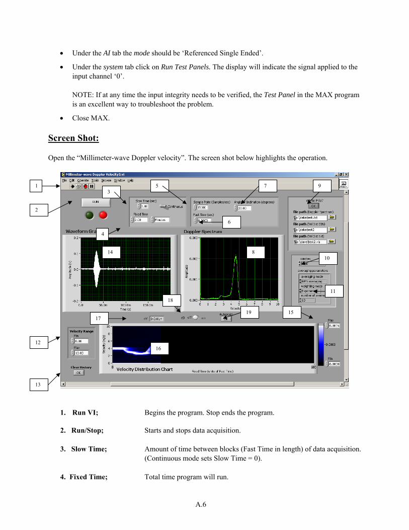
• Close MAX. Screen Shot: Open the “Millimeter-wave Doppler velocity”. The screen shot below highlights the operation.
1. Run VI; Begins the program. Stop ends the program. 2. Run/Stop; Starts and stops data acquisition.
3. Slow Time; Amount of time between blocks (Fast Time in length) of data acquisition.
(Continuous mode sets Slow Time = 0).
4. Fixed Time; Total time program will run.
1
2
3
4
5
6
7
8
9
10
12
13
14
15
16
11
17
18
19
A.7
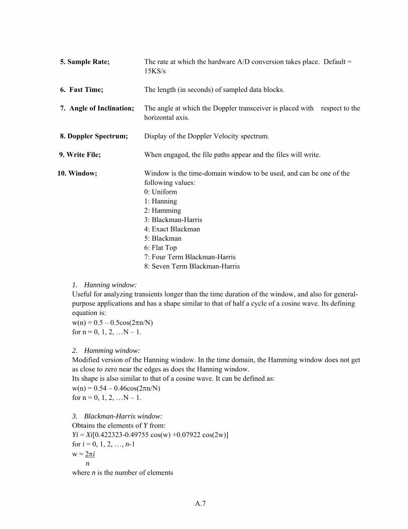
5. Sample Rate; The rate at which the hardware A/D conversion takes place. Default =
15KS/s
6. Fast Time; The length (in seconds) of sampled data blocks.
7. Angle of Inclination; The angle at which the Doppler transceiver is placed with respect to the horizontal axis.
8. Doppler Spectrum; Display of the Doppler Velocity spectrum.
9. Write File; When engaged, the file paths appear and the files will write.
10. Window; Window is the time-domain window to be used, and can be one of the following values: 0: Uniform 1: Hanning 2: Hamming 3: Blackman-Harris 4: Exact Blackman 5: Blackman 6: Flat Top 7: Four Term Blackman-Harris 8: Seven Term Blackman-Harris
1. Hanning window: Useful for analyzing transients longer than the time duration of the window, and also for general-purpose applications and has a shape similar to that of half a cycle of a cosine wave. Its defining equation is: w(n) = 0.5 – 0.5cos(2πn/N) for n = 0, 1, 2, …N – 1.
2. Hamming window: Modified version of the Hanning window. In the time domain, the Hamming window does not get as close to zero near the edges as does the Hanning window. Its shape is also similar to that of a cosine wave. It can be defined as: w(n) = 0.54 – 0.46cos(2πn/N) for n = 0, 1, 2, …N – 1.
3. Blackman-Harris window: Obtains the elements of Y from: Yi = Xi[0.422323-0.49755 cos(w) +0.07922 cos(2w)] for i = 0, 1, 2, …, n-1 w = 2πi
n where n is the number of elements
A.8
4. Exact Blackman: Obtains the elements of Y from: Yi = Xi[a0-a1 cos(w) + a2 cos(2w)] for i = 0, 1, 2, …, n-1 w = 2πi
n where n is the number of elements a0 = 7938/18608 a1 = 9240/18608 a2 = 1430/18608. 5. Blackman window: Obtains the elements of Y from: Yi = Xi[0.42-0.50 cos(w) +0.08 cos(2w)] for i = 0, 1, 2, …, n-1 w = 2πi
n where n is the number of elements
6. Flat Top Has the best amplitude accuracy of all the window functions. The increased amplitude accuracy (± 0.02 dB for signals exactly between integral cycles) is at the expense of frequency selectivity. The Flat Top window is most useful in accurately measuring the amplitude of single frequency components with little nearby spectral energy in the signal. The Flat Top window can be defined as: w(n) = a0 – a1*cos(2πn/N) + a2*cos(4πn/N) – a3*cos(6πn/N) + a4*cos(8πn/N), where a0 = 0.21557895 a1 = 0.41663158 a2 = 0.277263158 a3 = 0.083578947 a4 = 0.006947368.
11. Averaging Parameters:
Averaging mode: 1: No averaging 2: RMS averaging 3: Vector averaging 4: Peak hold.
RMS averaging: Provides an estimate of the true signal and noise levels in the input signal. Vector Averaging: Allows better noise rejection when the target signal is constant and the noise is random
A.9
Weighting Mode: Specifies the weighting mode for RMS and Vector averaging
Exponential: the averaging process is continuous
Linear: the averaging process stops once the selected number of averages has been computed
Number of Averages: The number of averages used during averaging.
12. Velocity Range; Min and max values for the Y-axis (velocity) of the Velocity Distribution
chart.
13. Clear History; When the button is pushed, the Velocity Distribution chart history will be removed from memory once the program is started or restarted.
14. Waveform Graph; Display of the input waveform prior to processing.
15. Velocity Distribution Min and max values for the Z-axis (amplitude) of the
Z Range; Velocity Distribution chart. 16. Velocity Distribution Displays the Velocity Distribution vs. scrolling time chart;
(which is in units of Fast Time). 17. dv; The change in velocity for discreet points on the display charts (displayed for reference). 18. dB on/off; Switches between normal and decibel mode. 19. Autoscale; Initiates auto scaling of the Doppler Spectrum graph and Velocity
Distribution chart. (This feature is best used for finding the signal range before manually setting the range).
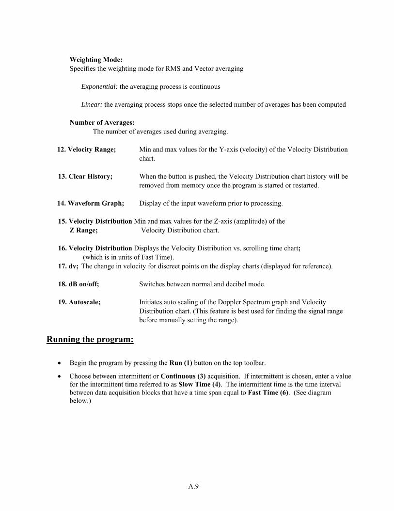
Running the program:
• Begin the program by pressing the Run (1) button on the top toolbar.
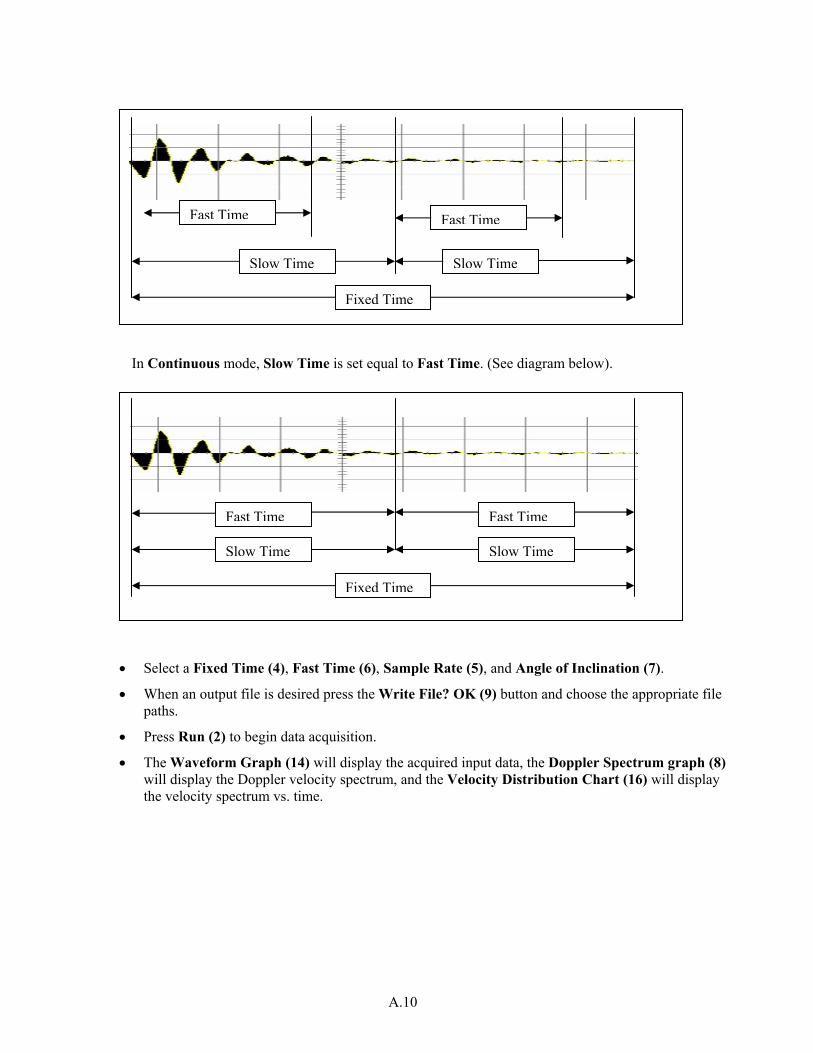
• Choose between intermittent or Continuous (3) acquisition. If intermittent is chosen, enter a value for the intermittent time referred to as Slow Time (4). The intermittent time is the time interval between data acquisition blocks that have a time span equal to Fast Time (6). (See diagram below.)
A.10
In Continuous mode, Slow Time is set equal to Fast Time. (See diagram below).
• Select a Fixed Time (4), Fast Time (6), Sample Rate (5), and Angle of Inclination (7).
• When an output file is desired press the Write File? OK (9) button and choose the appropriate file paths.
• Press Run (2) to begin data acquisition.
• The Waveform Graph (14) will display the acquired input data, the Doppler Spectrum graph (8) will display the Doppler velocity spectrum, and the Velocity Distribution Chart (16) will display the velocity spectrum vs. time.
Fixed Time
Slow Time Slow Time
Fast Time Fast TimeFast Time
Fast Time Fast Time
Fixed Time
Slow Time Slow Time
A.11
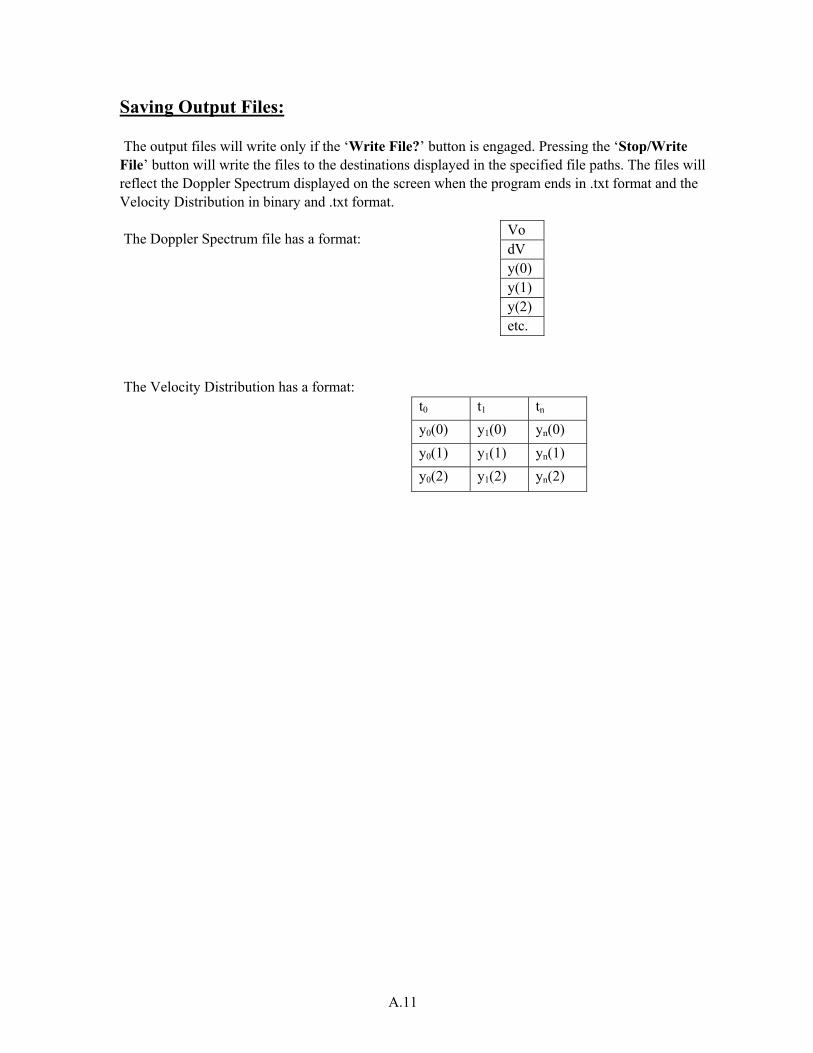
Saving Output Files: The output files will write only if the ‘Write File?’ button is engaged. Pressing the ‘Stop/Write
File’ button will write the files to the destinations displayed in the specified file paths. The files will reflect the Doppler Spectrum displayed on the screen when the program ends in .txt format and the Velocity Distribution in binary and .txt format. The Doppler Spectrum file has a format: The Velocity Distribution has a format:
t0 t1 tn
y0(0) y1(0) yn(0) y0(1) y1(1) yn(1) y0(2) y1(2) yn(2)
Vo dV y(0) y(1) y(2) etc.
A.12
Verification of the Output of the Millimeter-Wave Doppler Velocity Measurements for Gas-Solid Flows LabVIEW Program
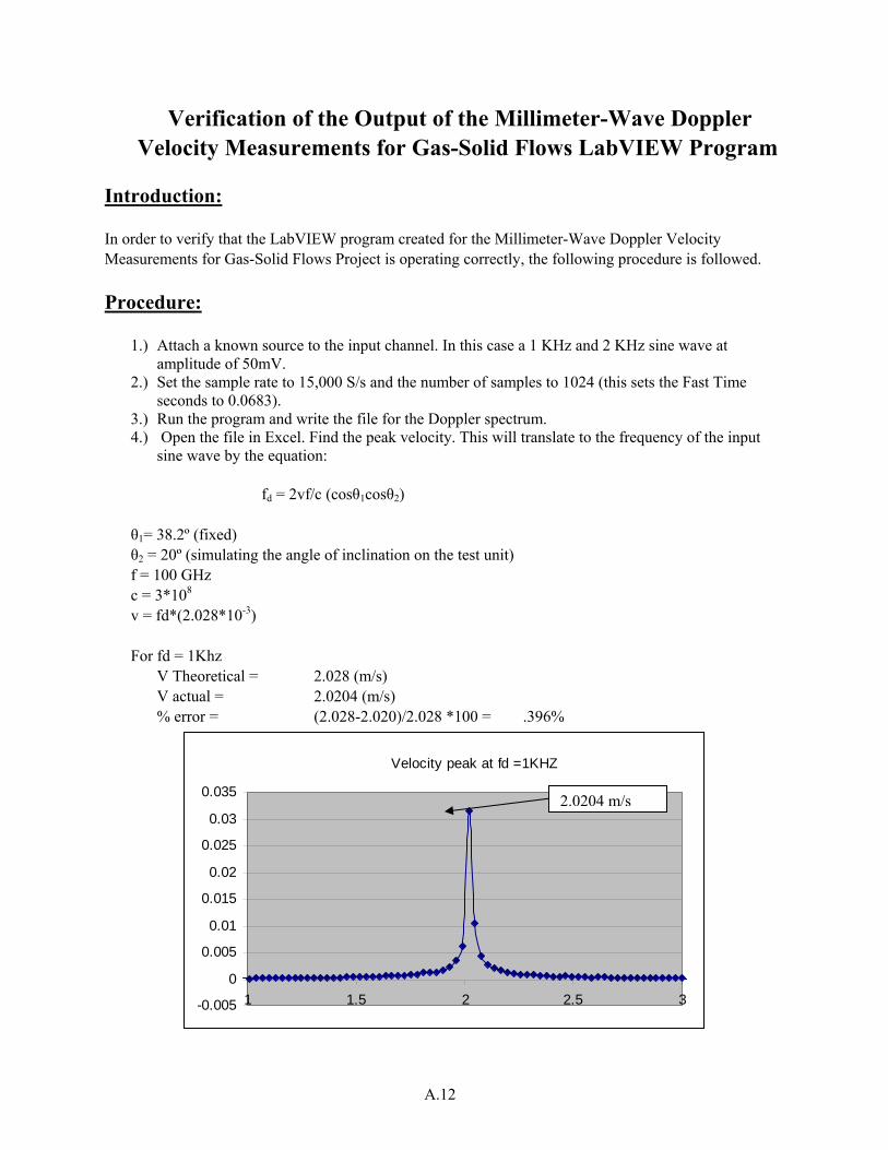
Introduction: In order to verify that the LabVIEW program created for the Millimeter-Wave Doppler Velocity Measurements for Gas-Solid Flows Project is operating correctly, the following procedure is followed. Procedure:
1.) Attach a known source to the input channel. In this case a 1 KHz and 2 KHz sine wave at amplitude of 50mV.
2.) Set the sample rate to 15,000 S/s and the number of samples to 1024 (this sets the Fast Time seconds to 0.0683).
3.) Run the program and write the file for the Doppler spectrum. 4.) Open the file in Excel. Find the peak velocity. This will translate to the frequency of the input
sine wave by the equation:
fd = 2vf/c (cosθ1cosθ2) θ1= 38.2º (fixed) θ2 = 20º (simulating the angle of inclination on the test unit) f = 100 GHz c = 3*108 v = fd*(2.028*10-3) For fd = 1Khz
V Theoretical = 2.028 (m/s) V actual = 2.0204 (m/s) % error = (2.028-2.020)/2.028 *100 = .396%
Velocity peak at fd =1KHZ
-0.005
0
0.005
0.01
0.015
0.02
0.025
0.03
0.035
1 1.5 2 2.5 3
2.0204 m/s
A.13
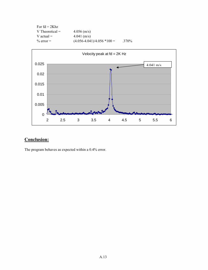
For fd = 2Khz V Theoretical = 4.056 (m/s) V actual = 4.041 (m/s) % error = (4.056-4.041)/4.056 *100 = .370%
Velocity peak at fd = 2K Hz
0
0.005
0.01
0.015
0.02
0.025
2 2.5 3 3.5 4 4.5 5 5.5 6
Conclusion: The program behaves as expected within a 0.4% error.
4.041 m/s