VALUE OF WALKABLE COMMUNITIES A Thesis … Thesis Presented to the faculty of the Department of Public Policy and Administration California State University, Sacramento Submitted in

VALUE OF WALKABLE COMMUNITIES

A Thesis

Presented to the faculty of the Department of Public Policy and Administration

California State University, Sacramento

Submitted in partial satisfaction of the requirements for the degree of

MASTER OF SCIENCE

in

Urban Land Development

by

Corina Cisneros

FALL 2015


A Thesis

by

Corina Cisneros Approved by: __________________________________, Committee Chair Robert Wassmer __________________________________, Second Reader Edward Lascher ____________________________ Date

ii

Student: Corina Cisneros

I certify that this student has met the requirements for format contained in the University

format manual, and that this thesis is suitable for shelving in the Library and credit is to

be awarded for the thesis.

__________________________, Department Chair ___________________ Edward Lascher Date Department of Public Policy and Administration

iii

Abstract

of


by

Corina Cisneros

The intent of this research is to determine what factors create walkable

communities, and for the information learned to be a useful tool to promote community

change with the goal of sustainable community design. One part of creating sustainable

communities is knowledge on the degree of walkability because this community feature

ties into so many other aspects of the health, social, and environmental concerns of a

community. Increased awareness and investment in walkable communities promotes

change that benefits individuals, communities, and society as a whole.

This thesis demonstrates the importance of walkability in sustainable community

design and how it can fit in with long range planning and policy directives supported at

the national, state, and local level. Analysis of the association between home values in the

Sacramento area and the degree of walkability of a home using Walk Score indicated

limitations with the data set. Based on the limitations found during this research I propose

an empirical measure of walkability that can be applied as a planning and development

tool to create walkable communities. The goal is to further explore the link between

residential land values and walkable communities. iv

_______________________, Committee Chair Robert Wassmer _______________________ Date

v

ACKNOWLEDGEMENTS

Thank you to my brothers Matias, Nathan, and especially Jacob. Jacob was like a second

parent to my daughter as I attended night classes to obtain my degree. Thank you to Rob

Wassmer for your continued guidance, patience, and understanding. Thank you Ted

Lascher for stepping in late in the process to assist as a second reader. Thank you to my

friends Alison, Davina, Jenny, and Victoria for always being there and for providing

support and encouragement. Thank you to Eli Harland and Ken Konecny, you two were

the best group partners in the program. I learned so much from the both of you. Thank

you to my husband Carlos for your support and willing to give me time to work the many

late nights. Thank you to my daughter Cienna. She is my motivation and my heart. My

time with her has been sacrificed as I forged to make a better life for us through higher

education and attainment of my master’s degree. Finally, words cannot express the

thanks due to my mother Monica. She has always been there for me no matter what

obstacles I have had in my life. She has encouraged me to be successful, to try my

hardest and be the best at what I do. She is the reason I have obtained a higher degree and

why I continue to strive to better myself. I love you mom.

vi

TABLE OF CONTENTS Page

Acknowledgements ..................................................................................................... vi

List of Tables .............................................................................................................. ix

List of Figures ............................................................................................................... x

Chapter

1. THE IMPORTANCE OF WALKABLE COMMUNITIES……………….…….. 1

Walk Score and Sacramento Real Estate Market ............................................. 4

Overview of the Remainder of this Thesis .......................................................7

2. LITERATURE REVIEW OF WALKABILITY: BENEFITS, HEDONIC PRICE

MODEL AND WALK SCORE ............................................................................ 10

Benefits of Walkability ................................................................................... 10

Hedonic Price Model ...................................................................................... 16

Walkability and Walk Score……………………………………………….. 20

3. REGRESSION ANALYSIS: WALK SCORE AND SACRAMENTO HOME

SALE PRICE ....................................................................................................... 28

Hedonic Regression Model ............................................................................. 28

Data Sources ................................................................................................... 36

4. FINDINGS AND INTERPRETATIONS ............................................................. 42

Initial Regression ............................................................................................ 42

Selection of Functional Form.......................................................................... 46

vii

Regression Analysis Errors ............................................................................. 48

Discussion ………………………………………………………………….. 50

New Walkability Measure .............................................................................. 51

5. AN ALTERNATIVE WALKABILITY MEASURE ........................................... 53

Walk Score Limitations .................................................................................. 55

An Alternative Walkability Measure .............................................................. 56

Policy Implications ........................................................................................ 59

References ........................................................................................................... 61

viii

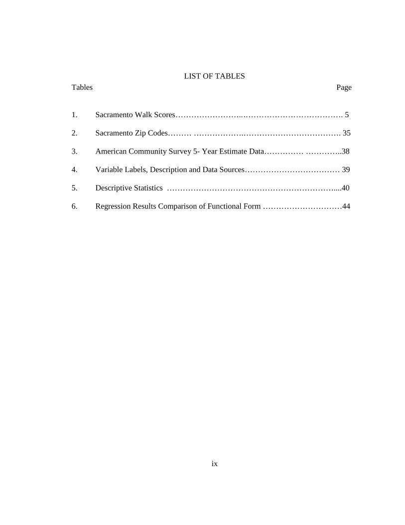
LIST OF TABLES Tables Page

1. Sacramento Walk Scores…………………….. .………………………………. 5

2. Sacramento Zip Codes……… ……………….………………………………. 35

3. American Community Survey 5- Year Estimate Data…………… …………..38

4. Variable Labels, Description and Data Sources……………………………… 39

5. Descriptive Statistics ………………………………………………………....40

6. Regression Results Comparison of Functional Form …………………………44

ix

LIST OF FIGURES Figures Page

1. United States Obesity Trend 1990, 2000, 2010.………………………………. 13

2. Scatterplot Linear Relationship……………….………………………………. 42

x

1

Chapter 1

THE IMPORTANCE OF WALKABLE COMMUNTIES

As a child growing up in Southern California I experienced traffic, pollution, and

overcrowding. I can still vividly remember days when we were not allowed to play

outside because the air pollution was so bad it would make us sick. My family lived in

the San Fernando Valley and I still recall knowing it was a clear beautiful day when we

could see the mountains that surrounded the valley, most of the time there was a thick

haze limiting our view. Based on these observations as a child I knew the greater Los

Angeles area was not good place to live. As I grew older and began college did I really

begin to understand why Los Angeles developed the way it did. I began to reflect about

the development policies that government’s support and how certain policies can have a

lasting and profound effect on the development of cities. One can only imagine how

Southern California would have developed if the powers that be had continued to expand

the trolleys and other public transportation networks, focused development on walkable

communities, and less investment on freeways and private automobile transportation.

Perhaps the greater Los Angeles area would be a model of health and vibrancy instead of

the sprawl and congestion we know it now to be.

The desire for changing the way cities, communities, and neighborhoods develop

from this point forward have been vocalized by policy makers at the federal, state and

local level. At the federal level incremental changes in policy and directives have called

for the creation and support of more walkable communities. The following quote

2

summarizes the idea envisioned in this thesis “Walkable communities are urban places

that support walking as an important part of people’s daily travel through a

complementary relationship between transportation, land use and the urban design

character of the place. In walkable communities, walking is a desirable and efficient

mode of transportation” (Institute of Transportation Engineers, 2012, p. 64).

The federal Department of Transportation (DOT) Bicycle and Pedestrian Program

announced a policy statement in Spring 2010 for support and development of an

integrated transportation network which included connected walking and biking

networks, “Walking and bicycling foster safer, more livable, family-friendly

communities; promote physical activity and health; and reduce vehicle emissions and fuel

use” (www.dot.gov) In conclusion the policy statement indicated that although DOT can

be the leader with its federal directives and support, it is ultimately up to the

transportation agencies across the nation to implement the policies. The agency with the

greatest impact on national housing development and direction, The U.S. Department of

Housing and Urban Development (HUD) has also acknowledged the need to create

walkable communities that are healthier for people and the environment. In partnership

with DOT and the Environmental Protection Agency (EPA), HUD’s Office of

Sustainable Housing and Communities has coordinated the offer of Sustainable

Communities Planning Grants “…In order to better connect housing to jobs, the office

will work to coordinate federal housing and transportation investments with local land

use decisions in order to reduce transportation costs for families, improve housing

3

affordability, save energy, and increase access to housing and employment opportunities

(www.hud.gov)”. Under federal direction there has been a growing awareness to change

policy and planning in regards to urban planning, transportation planning, and

environmental stewardship, but as indicated by the DOT, responsibility for action and

real change must be implemented by individual states and communities.

This thesis will demonstrate the importance of walkability in sustainable

community design and how it can fit in with long range planning and policy directives

supported at the national, state, and local level. Ultimately, this thesis will analyze the

association between home values in the Sacramento area and the degree of walkability of

a home. Ultimately, I will propose an empirical measure of walkability that can be

applied as a planning and development tool to create walkable communities. The purpose

is to further explore the link between residential land values and walkable communities.

If there is in reality a premium for homes in walkable communities, this will help support

the policy directives highlighted previously at all levels of government. It will also help

housing consumers to make educated decisions on where they choose to vote with their

housing dollars, walkable communities or car dependent ones, and will send a message to

developers and the public agencies in support of development how best to plan and

prioritize funding. The remainder of this chapter will introduce the Walk Score

walkability measured examined in this thesis; the housing and demographic market of

Sacramento; and concludes with the specific research questions and description of the

remaining chapters in this thesis.

4

Walk Score and Sacramento Real Estate Market

Walk Score was developed in 2007 with the stated mission “to promote walkable

neighborhoods. Walkable neighborhoods are one of the simplest and best solutions for

the environment, our health, and our economy” (walkscore.com). The website states

Walk Scores are shown for over 20 million locations every day and are used on over

30,000 sites. Walk Scores are given for a location with a number of how walkable that

location is from 0-100 scale.

Walk Scores

90-100- Walker’s Paradise- daily errands do not require a car.

70-89 Very Walkable- most errands can be accomplished on foot.

50-69 Somewhat Walkable- some errands can be accomplished on foot

25-49 Car Dependent- most errands require a car.

0-24- Care Dependent- almost all errands require a car.

(https://www.redfin.com/how-walk-score-works)

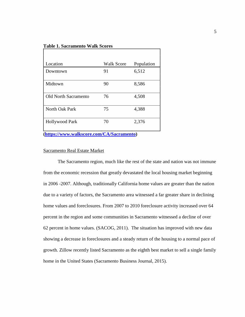
The following table information was taken directly from Walk Scores website for

Sacramento. Sacramento as a whole Walk Score is 43 which is considered Car

Dependent. Individual communities in Sacramento are listed below. As shown those

locations closer to the central business district have a higher Walk Score. Both

Downtown and Midtown are considered a Walker’s Paradise. This is evident from

anyone with familiar with these areas due to the shops, restaurants and other amenities

within close walking distance.

5

Table 1. Sacramento Walk Scores Location Walk Score Population Downtown 91 6,512 Midtown 90 8,586 Old North Sacramento 76 4,508 North Oak Park 75 4,388 Hollywood Park 70 2,376

(https://www.walkscore.com/CA/Sacramento)

Sacramento Real Estate Market

The Sacramento region, much like the rest of the state and nation was not immune

from the economic recession that greatly devastated the local housing market beginning

in 2006 -2007. Although, traditionally California home values are greater than the nation

due to a variety of factors, the Sacramento area witnessed a far greater share in declining

home values and foreclosures. From 2007 to 2010 foreclosure activity increased over 64

percent in the region and some communities in Sacramento witnessed a decline of over

62 percent in home values. (SACOG, 2011). The situation has improved with new data

showing a decrease in foreclosures and a steady return of the housing to a normal pace of

growth. Zillow recently listed Sacramento as the eighth best market to sell a single family

home in the United States (Sacramento Business Journal, 2015).

6

As the real estate market becomes less volatile and consistency and growth return

to normal it is imperative that planners, policy makers, and government officials

recognize the need to accommodate developments that are more reflective of changing

preferences and demographics. A variety of research has identified factors such as an

aging and significant baby boomer population that does not prefer large lot single family

housing and the current younger generation that desires housing close to work, shopping,

and dining. The Director of the Metropolitan Research Center at the University of Utah

Arthur Nelson’s research suggests that over half of the developments in 2025 will not

have existed in 2000 due to changing land use patterns and the preference of the two

groups identified previously. He identifies the need for housing units such as apartments,

town homes, and condos and small lot-houses in the future (SACOG, 2010). Jonathan

Rose the CEO of a national development and investment firm states, “It is very unlikely

that new projects in sprawl areas will be financed. Urban areas with diverse transit

options and thriving universities are the choice for Baby Boomers and young people

(Leinberger, 2010)”.

In addition to the policy and demographic changes, actual consumers are

demanding a shift from current housing types. A preference is indicated all over the

country for sustainable, smart growth, and walkable communities. In the winter 2010

National Association of REALTORS (NAR) publication “On Common Ground”, the

focus was on ‘green communities’. From Florida to Oregon realtors are noting the public

desire for walkable communities. A pendulum shift is occurring in the real estate market

7

where a premium is placed on homes in walkable communities versus auto-orientated

suburbs. One REALTOR summarized this shift as not merely a trend but a new way of

life. A Portland, Oregon REALTOR explained from personal experience her clients “Are

willing to pay more for a home – or accept less in terms of square footage and amenities

– in exchange for proximity to shopping, entertainment, work and school (On Common

Ground, 2010).” A 2011 survey by NAR also indicates consumer preference for walkable

communities. It was found 56 percent of Americans prefer walkable mixed used

neighborhoods over ones that where they have to drive more between work and home

(NAR 2011).

The Sacramento region is not exempt from these changing demographics and

regional plans, the Sacramento Area Council of Governments (SACOG) a regional

planning organization in the area developed the in process Metropolitan Transportation

Plan/Sustainable Communities Strategy 2035, which identifies the need for future growth

to shift towards developments closer to work and services, smaller lots and attached units

and increased rental units to satisfy demand (SACOG, MTP/SCS 2035). Growth is

predicted to shift from 35 percent single-family small lot and attached units and 65

percent single family large-lot in 2008 to 62 percent and 38 percent respectively by 2020.

This represents a complete turnaround in the future development of communities in the

region.

8

Overview of the Remainder of this Thesis

State laws are demanding a new way of planning and development. At the

individual level people are demanding the creation of walkable communities. Taken

together the writing is clear, a shift towards revitalizing existing communities towards

walkability as well as planning for new developments with the same focus is paramount

to our success as a nation, state, city and finally community. One area that can address

both the health and environmental welfare of our region is to develop tools that promote

walking not only as a source of physical activity but encourage it as a sustainable

transportation mode for work and leisure. The research agenda for this thesis is the

starting point on which to formulate policies and objectives aimed at identifying those

places in which to focus incentives for creating walkable, sustainable communities.

Specifically, this thesis will analyze the relationship between homes values and

Walk Score in select neighborhoods within the City of Sacramento and to systematically

evaluate whether Walk Score as a measure of walkability alone should be applied as a

planning tool to combat the negative associations of sprawl and poor planning discussed

previously. My prior research on this subject has indicated homes in walkable

neighborhoods can command a premium in the housing market, but as with any research

more analysis and variables are needed to determine if Walk Score alone should be

applied to determine the best measures of walkability. What this thesis will do is evaluate

Walk Score, discuss the criticisms found in my prior research as well as new research and

9

empirically formulate a method of measuring walkability as planning and development

tool.

The thesis is organized as follows. In Chapter 2 I will present a Literature Review

to acquaint the reader with previous research on this topic as well as provide a basis for

comparison to different research models. This chapter will discuss relevant research on

walkability as a planning tool, the research utilizing Walk Score, and limitations and

criticism of Walk Score research. Chapter 3 details the methodology used in this thesis to

generate the Walk Score regression. I used an Ordinary Least Squares (OLS) regression

model to determine the relationship between home value and Walk Score. This chapter

provides a clear understanding of the explanatory variables chosen and their anticipated

influence on home value, and indicates the data and sources used in the thesis which is

compiled in a data table format to allow for ease of dissemination and discussion. In

Chapter 4 the results of the regression analysis are reviewed and explained. Chapter 4

organizes the results obtained from the analysis and discusses the findings, and proposes

an empirical way to measure walkability that does limit walkability measurements strictly

to Walk Score data. Chapter 5 concludes with reflections on the regression model, how to

interpret the significant results, and suggestions for improving Walk Score or starting

fresh with a new empirical measure of walkability that can be applied to promote change

for future policy directions and initiatives.

10

Chapter 2

LITERATURE REVIEW OF WALKABILITY: BENEFITS, HEDONIC PRICE

MODEL, AND WALK SCORE

This chapter will be organized around four main themes: 1) the benefits of

walkable communities, 2) the nature of the hedonic price model and relevant literature on

neighborhood design characteristics that may influence walkability, 3) research on

walkability and Walk Score, and finally 4) limitations of Walk Score. The focus of the

literature review will be to discuss the findings of each theme and how they relate to

walkability. This is done with an eye toward formulating a new methodology for

walkability and its role in home value.

Benefits of Walkability

This chapter begins with a review of the benefits of walkability found in research

literature. I believe intuitively many people know there are benefits of walking and

exercise in general. We know we feel better when we move our bodies, but what

specifically are the benefits of communities that promote walking as a form or transport

and leisure? The answer to this question is important because if one is to develop a

comprehensive model that measure walkability, one must know how that measure is

intended to facilitate acquisition of specific benefits.

Academic research has examined the link between walkability and desirable

community design. Fueling this growing academic research field are concerns about the

health of the nation, environmental degradation, and a desire by many in the planning

11

profession to address these circumstances with focus and attention on sustainable

communities (Giles-Corti et al, 2015, Giles-Corti et al, 2014, Pivo & Fisher, 2011).

Walkable communities are one part of this dynamic of creating vibrant, healthy, and

livable places. The walkability of a community is an essential component of sustainable

community design and the health, social, and environmental benefits are indicators of

overall community health and vibrancy.

Health Benefits

There is a growing amount of research and data to support the claim that walkable

communities can be an important aspect of a healthy active lifestyle (Lovasi, Grady, and

Rundle, 2012, Duncan et al, 2011, Giles et al, 2009, Saelens & Handy, 2008). Our society

is battling a growing epidemic of health diseases and problems attributed to a sedentary

lifestyle (Pivo & Fisher, 2011). Estimates indicate physical inactivity is responsible for

over five million deaths annually throughout the world (Giles-Corti et al, 2015).

Obesity accounts for many health problems such as cardiovascular disease, cancer and

diabetes. Information obtained from the Centers for Disease Control (CDC) on health

risks such as obesity facing Californians, and specifically people living in the U.S.

Census defined Sacramento Metropolitan Statistical Area, indicate alarming rates of the

population battling these health problems (www.cdc.gov). However, the link between

the built environment and the degree of physical activity that communities engage in

increasingly shows a relationship (Giles-Corti et al, 2015, Frank et al, 2004, Goldberg,

2007, Saelens & Handy 2008). Built environments and communities that encourage

12

walking and biking can have a positive impact by addressing physical inactivity and

sedentary lifestyles according to information obtained from the Alliance for Biking and

Walking 2012 Benchmarking Report (Bicycling and Walking in the United States 2012

Benchmarking Report). The report provides reliable and relevant data to government and

elected officials to base support and sound decision-making for policies to increase

walking and biking as a viable transportation alternative to car use. What makes this

report unique and worth discussing is the specific data about Sacramento. Sacramento

ranks third in per capita spending of federal money for bicycling and walking between

the years 2006-2010 and ranks fifteenth for bicycle and walking levels in the same years

(Bicycling and Walking in the United States 2012 Benchmarking Report, 2012).

The nation has seen alarming growth in the number of overweight and obese

people, especially among children and young adults. Analyzing data going back to the

1960s, the Alliance for Biking and Walking 2012 report shows that as Americans have

decreased their use of walking and biking as a transportation option, the percent of

Americans classified as obese soared (2012 Benchmark Report). Based on the 1960

Census and CDC data almost ten percent of trips to work was by walking and the obesity

rate for adults was less than fifteen percent. By 2009 the obesity rate for adults nearly

reached thirty-five percent of the population, and walking or biking to work was down to

less than four percent of trips. For children the data is similar. Beginning with the years

1966-1969 the obesity rate for children was around four percent and the percent of kids

who walked or biked to school was almost forty-five percent. By 2009 the obesity rate for

13

children was close to eighteen percent and the percent of kids who walked or biked to

school had fallen to around ten percent (Benchmark 2012).

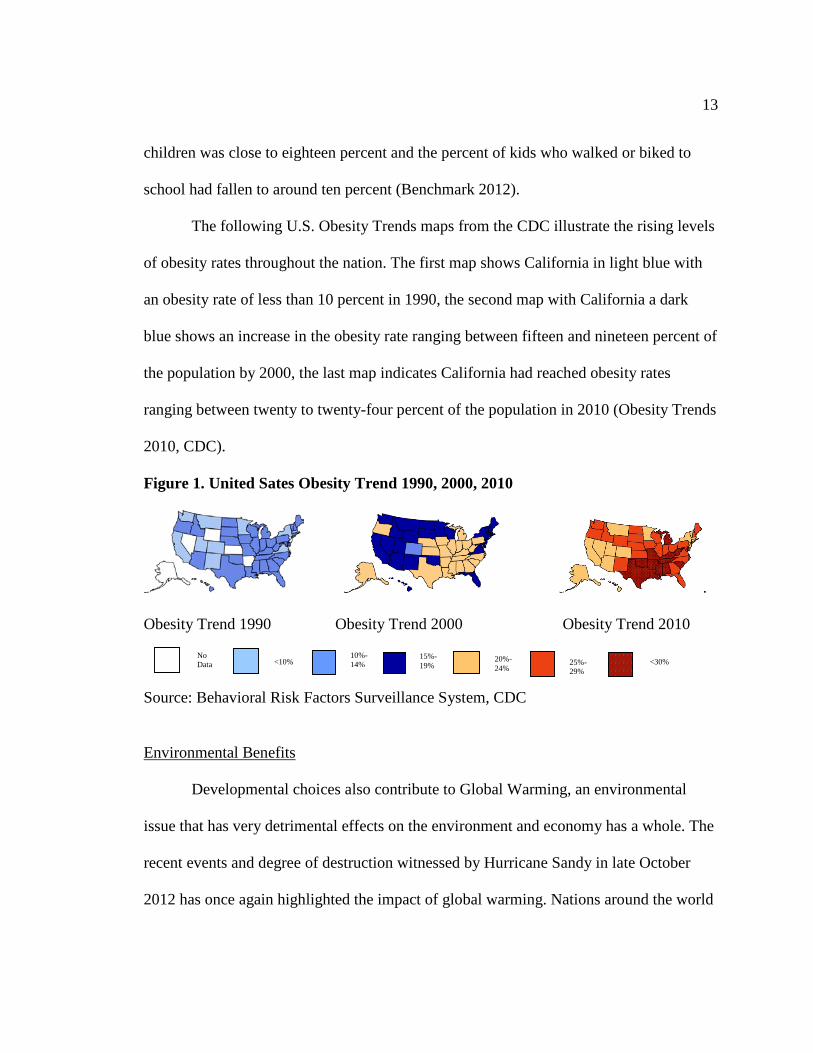
The following U.S. Obesity Trends maps from the CDC illustrate the rising levels

of obesity rates throughout the nation. The first map shows California in light blue with

an obesity rate of less than 10 percent in 1990, the second map with California a dark

blue shows an increase in the obesity rate ranging between fifteen and nineteen percent of

the population by 2000, the last map indicates California had reached obesity rates

ranging between twenty to twenty-four percent of the population in 2010 (Obesity Trends

2010, CDC).

Figure 1. United Sates Obesity Trend 1990, 2000, 2010

. Obesity Trend 1990 Obesity Trend 2000 Obesity Trend 2010 Source: Behavioral Risk Factors Surveillance System, CDC

Environmental Benefits

Developmental choices also contribute to Global Warming, an environmental

issue that has very detrimental effects on the environment and economy has a whole. The

recent events and degree of destruction witnessed by Hurricane Sandy in late October

2012 has once again highlighted the impact of global warming. Nations around the world

No Data <10%

10%-14%

15%-19%

20%-24%

25%-29%

<30%

14

are implementing measure to curb their output of greenhouse gases (GHG), which

contribute to global warming. The warming of the Earth’s atmosphere is attributed to

certain gases that stay in our environment and act as a blanket, trapping heat generated

from the earth in and not allowing warming gases to escape. This in turn causes

temperatures to rise. Not all GHG are bad; without them the Earth’s temperature would

be significantly lower, making for a dramatically different type of environment. The main

GHG are water vapor, carbon dioxide (CO2) and methane. Of the three main gases

carbon dioxide is the one countries, cities, and states are effectively trying to reduce.

Carbon dioxide levels have continued to rise over the last one hundred years and will

continue to rise long after people implement drastic measure to limit their output into the

atmosphere.

The consumption of fossil fuel energy is the single largest contributor of

greenhouse gas emissions for the world and carbon dioxide is responsible for 81% of

total U.S. greenhouse gas emissions (EIA, 2009). The number one contributor of carbon

dioxide emissions is transportation, which is closely tied to development, especially

sprawling green field developments. In the United States transportation accounts for

about 33% of total U.S. energy related GHG emissions, followed by the residential and

commercial sector with 26% of the emissions. The residential, commercial, and

transportation sectors combined account for close to sixty percent of GHG emissions, and

indicate the need for change in the way we travel and how we live (EIA, 2009). These

figures were obtained from the Department of Energy’s Energy Information

15

Administration (EIA), Green House Gas Emissions Report, 2008. Data from the report

indicates an overall decrease in 2008 GHG emissions by 2.2 percent from 2007 totals. A

combination of factors contributed to the lowering, the economic recession and increase

in fuel prices, causing consumers to tailor back their usage.

The urgency in reducing greenhouse gases, especially carbon dioxide is

increasingly becoming more important to the overall functioning of the State of

California. The state realizes the economic, social and global importance of tying to

mitigate the effects of global warming. Part of this commitment is directly tied to

modifying current building practices and energy consumption which contribute

significantly to global warming. Urban and regional planning can encourage development

in ways that encourage walkable communities or continue with developments that

essentially assure dependence on auto use.

California has been a leader in support of recognizing and seeking solutions to

mitigate decades of misguided transportation and planning policy. Historical legislation

passed such as AB 32 - The Global Warming Solutions Act and SB 375 - The

Transportation and Land Use Planning Bill set new goals for California to move towards

a sustainable future. According the Office of the Governor Fact Sheet on SB 375, “SB

375 provides incentives for creating attractive, walkable, sustainable communities and

revitalizing existing ones. It will encourage the development of more alternative

transportation options. By doing so, this law will promote healthy lifestyles…

(www.gov.ca).” Due to these key pieces of state legislation, communities finally have to

16

adopt long ranging planning and development plans that are sustainable and

fundamentally smarter for society in the long term.

The next section will discuss the hedonic price model. This is important to explain

how a home’s value is determined. An understanding of the model is needed to explain

why walkability should be part of home valuation.

Hedonic Price Model

Hedonic Model

There are a number of factors that affect the price of a home such as location,

housing characteristics, and land prices, to name a few. One can think of a house as a

basket containing many goods. Each of the goods plays a part in determining the basket’s

value. Economic research on home values often use a method of “hedonic” home

valuation developed in the 1970’s by Rosen (Gibbons & Machin, 2008). The hedonic

prices modes use a statistical regression analysis to arrive at a value for a home. This

statistical analysis determines home value derived from other variables and their

influence or impact on value. The hedonic framework in housing analysis is a useful tool

to determine the value of various housing characteristics and their impact on price.

Housing is not a uniform good, and simply comparing prices would not capture site

specific attributes that play a part in price (Cotright, 2009). Hedonic analysis essentially

unbundles the various components of a home and estimates a price for each; the value of

the house is a composition of the various characteristics (Rosen, 1974). House price can

be seen as function of some basic components, such as structural characteristics which

17

include number of bedrooms, number of bathrooms, age and lot size (Cotright, 2009).

Neighborhood characteristics include distance to school, transportation accessibility,

environmental factors, crime, and other location factors which can all influence the value

of a home. (Gibbons & Machin, 2004).

Some of the more widely studied effects on housing price include evaluation of

schools, transportation and crime. A review of the literature on these aspects undertaken

by Gibbons and Machin (2008) aimed to determine components of these characteristics

on property values. They show quality schools generally have a positive influence on

home price, but the degree of the influence varies across the 14 studies included in their

review. Magnitudes on home value from the studies range from a low of 1.3 percent

increase for one-standard deviation increases in math scores to a high of a 10 percent

increase for one-standard deviation of a school receiving and ‘A’ grade. The author’s

own study in 2006 results in a 3.8 percent increase in home value for a one-standard

deviation increase in school performance (Gibbons & Machin, 2008).

Transportation accessibility was also found to be a key component of property

value. The closer a home is to transportation connections or rail transit the greater value.

Home within walking distance to rail and transit lines are valued at a premium. The

Gibbons & Machin study found a 7-20 percent decrease in home value for one-standard

deviation increase in home distance to transit station (Gibbons & Machin, 2008). The

authors also cited another significant study by Armstrong and Rodriguez (2006)

indicating a 10 percent premium for properties within a ½ mile of station and a 15

18

percent reduction in home value per minute with increasing home-station drive time

(Gibbons & Machin, 2008).

The impact on housing values due to crime seems intuitive: the more crime in the

area where a home is located, the less the value of that home. One study conducted in

New York City determined that a fall in violent crime rates by 13% does in fact lead to

about an 8% increase in property values. These values were statistically significant with

81% of the variation in home prices explainable by the model (Schwartz, Susin and

Voicu, 2003). The period for the study is somewhat dated: property values and crime

statistics were gathered in a ten-year period from 1988-1998. However, the indications

from the study remain valid.

Neighborhood Characteristics

In addition to the hedonic price model there are factors related to community

characteristics and design elements that influence housing price. These characteristics are

not part of the variables I will use in my regression, but their importance stems from

elements contained in their characteristics that encourage walking as a viable alternative

to auto dependence.

Several studies by Tu and Eppli (1999, 2001) have analyzed the degree of price

premiums for “New Urbanist” housing versus related suburban housing. In their study in

Kentlands, Washington D.C it was shown that price premiums from 4% to 15% could be

placed on housing in New Urbanist communities. Some of the features of New Urbanist

communities include connected streets, higher densities and a mix of land uses, which

19

can also be attributes of a walkable community (Cotright, 2009). New Urbanist

communities are designed with the principles of traditional neighborhood development

(TND) and in this study the measure of New Urbanist and TND are used interchangeably.

New Urbanist communities in the study were identified with the dummy variable TND

and coded 1 if the development is a TND and 0 otherwise. The values from the regression

were then compared to a similar regression using conventional neighborhood data, with

conventional referring to low-density, auto-oriented development. Other relevant

variables from this study included age, total number of bathrooms, dummy variable for a

single story, and lot size. All were shown to be statistically significant in this study. Lot

size and number of bathrooms showed the greatest influence on home value besides the

TND variable.

Prior work also has found mixed-use land development patterns also have a

positive effect on home values. Song and Knapp (2003) conducted a study aimed at

addressing the lack of research that quantifies home values in mixed-use communities in

spite of popular claims of their benefits, and to determine consumer preference for mixed

used developments (2003). The study measured the proximity to amenities such as

shopping and parks. The authors found that housing prices increase when located near

public parks (.3%) or neighborhood scale commercial centers (1%), but decrease when

located near multi-family housing or bus stops. Most importantly, the study found that a

premium can be charged for housing located within walking distance of parks or

commercial centers. It should be noted also that the scale of commercial centers is

20

important, housing values decrease when the intensity of commercial centers increases,

there must be balance between housing and commercial space (Song & Knapp, 2003).

Walkability and Walk Score

I now turn to an assessment of studies where walkability is a key component or

explanatory variable for housing price. At this point I would like to explain the

components of walkability that determine a Walk Score™, which is central to my own

research. Walk Score is a value derived from the popular website, www.walkscore.com.

This measure uses publicly available data to allow one to look up a specific location’s

walkability determined by distance from a specific location to nearby amenities.

Amenities are grouped and points are applied to the location based on the number of

amenities. Amenities a quarter of mile or less receive the highest points, with decreasing

points for increasing distances up to one mile. The categories are weighted and summed

providing a Walk Score value between 0-100, with 100 the best indicator of walkability.

An example of amenity categories includes restaurants, schools, parks, cultural centers,

etc. Walk Score also recently incorporated pedestrian friendliness by measuring

“population density road metrics such as block length and intersection density”.

(www.walkscore.com).

In the past, the use of Walk Score in academic literature was limited and few

articles existed in peer-reviewed journals. However, there has been a change in the

academic scene and increasingly articles have appeared which have successfully

integrated Walk Score values into valid research. A question one must ask, is the use of

21

Walk Score a valid and reliable indicator of walkability and thus for this analysis, a

premium component of residential home value? So far the research has indicated yes,

Walk Score can be a useful tool and is a valid measure of walkable neighborhoods that

does translate to increased property values (Gilderbloom, Riggs, and Meares, 2015,

Duncan, et al., 2011, Carr, Dunsiger, and Marcus, 2010 and 2011) Its use in popular

home real estate websites such as Zillow.com and Realtor.com also attest to its

significance and use by the larger public (Leinberger, 2010).

In a very recent study published in February 2015, researchers questioned whether

walkability matter and sought to examine its impact on housing values, foreclosures and

crime (Gilderbloom, et al., 2015). The subject city for their analysis was 170 census tracts

in Louisville, KY considered to be a mid-size city. The researchers chose to use Walk

Score™ as their key test variable because of the following stated advantages “While

many tools employ surveys, self-reporting audits and observational data measures, the

Walk Score™ tool provides a direct and replicable way of assessing geospatial,

population and land use characteristics to benchmark walkability” (Gilderbloom, et al.,

2015, p. 16). This study also discussed the limitations with Walk Score™ which will be

analyzed further in theme four. Significantly, the research found that walkability is

valued and should be incorporated into hedonic regression analysis for mid-sized cities

where it has not been used, and is associated with higher property values, less

foreclosures and reduced crime rates. The researchers state the value from walkability

can influence policy toward creating sustainable neighborhood design and that is does

22

matter when consumers are evaluating where to live along with schools, jobs, crime, and

transportation costs, (Gilderbloom, et al., 2015).

Christopher Leinberger, an author of several articles and books advocating for

walkable communities, completed a coauthored study for the Brookings Institute on the

walkability of places in Washington D.C (Leinberger and Alfonzo, 2012). The

methodology for their research including trying to establish performance metrics for

walkable urban places using a variety of secondary real estate, demographic,

transportation, and economic data. The study’s aim was to show that walkability could be

a mechanism to increase a place’s triple bottom line of people, planet, and profit. The

study employed the use of Walk Score initially to determine walkable places in D.C.

however do to limitations of Walk Score they ultimately used their own matrix based on

are more complete set of micro-scale built environmental features which promote

walking (Leinberger and Alfonzo, 2012). The limitations mentioned in this research and

other research utilizing Walk Score will be discussed in more detail in the fourth theme

of this literature review. The key finding in Lienberger’s and Alfonzo’s hedonic

regression study was that residential rental units in walkable places can command an

additional $301.76 per month in rents and for sale properties can add a $81.54/sq. ft.

premium in value for a 20-point increase in walkability from a range of 94 (Leinberger &

Alfonzo, 2012).

In another article researchers evaluated residential land values and walkability

(Rauterkus & Miller, 2011). Walk Score was calculated for over 5,000 property

23

transactions and were evaluated in one county in Alabama to determine the relationship

between residential land only values and walkability. This study is unique in that

residential land values and not building improvements were analyzed using an OLS

regression. The study found that controlling for population growth and lot size,

walkability as measured by Walk Score did in fact have a direct relationship to land

values. Land values in neighborhoods closer to the central business district (CBD), in

older communities, and located near universities having a high degree of walkability

which does increase land values (Rauterkus & Miller, 2011).

Another widely cited, non-academic study attempted to assess the impact of Walk

Score on home values (Cotright, 2009). Most of the academic literature available had

ignored walking as a form of transport in communities, and therefore the Cotright study

is important and worth mentioning. The study obtained Walk Scores for 92,276

properties in 15 metropolitan cities in the United States and found that those properties

with high Walk Scores are priced higher than a comparable home in 13 of the study cities

(Cotright, 2009). The most Significant finding was that in a typical market a one-point

increase in Walk Score translates to an increase of between $700 and $3000 in property

value (Cotright, 2009). Yet the study is plagued by offering little methodological

information, including how the properties and cities were chosen. While the study is

suggestive, the results must be viewed with caution.

Another study use examines the impact of Walk Score on commercial property

values and investment returns (Pivo & Fisher, 2011). According to the authors, an aspect

24

of sustainable and responsible property investing is the walkability of properties due to

the inherent social and environmental benefits of building walkable places. The study

used an OLS regression to evaluate the degree, if any, in which Walk Scores influence

commercial property values. The study found that a ten-point increase in walkability

increases property values between 1-9% dependent on property type, and walkable

properties generate higher incomes (Pivo & Fisher, 2011).

Finally, one study examined the degree that walking influences social capital

(Leyden 2003). According to the author, walkable communities encourage social

cohesion, political participation and builds trust (2003). However, the study suffered from

notable limitations, including a low response rate of the survey (279), which was

designed to capture data on the key variables. In addition, respondents were asked to

determine their walkability index based on a set of nine questions. Finally, the study took

place in Ireland, which can hinder the results from being applicable to U.S. communities.

In summary, the studies of the walkability of a location seems to indicate that a

premium in price is associated with walkability in commercial and residential markets as

well as increasing social capital.

Walk Score Limitations

The Walk Score also has notable limitations. It does not account for other

walkability factors such as safety, environmental, or topographic deterrence’s

(Gilderbloom, et al., 2015, Pivo and & Fisher, 2011, Carr, et al., 2010). Walk Score has

25

addressed the safety aspect limitation with its Crime Grade, but this is an independent

measure and it is not calculated in the Walk Score algorithm.

Perhaps the greatest limitation, and one currently being addressed by Walk Score,

is the straight line distance calculated from one location to another, not factoring in

attributes that facilitate walking such as street connectivity and route. The website now

has a beta version of what is called Street Smart, which calculates a Walk Score that

takes into account street connectivity and intersection density for a specific location

(www.walkscore.com).

Gilderblooms, Riggs, and Meares 2015 work in Louisville, KY highlight some of

the previously mentioned limitations identified with Walk Score including the straight

line distance calculations. This is an important aspect as people when walking do not

always have the ability to walk the shortest route from point A to point B. This limitation

was also identified in an article on the validation of Walk Score (Duncan, et al., 2011).

The consensus from the research indicates Walk Score can be useful to determine some

walkable places, but cannot be universally applied to measure overall neighborhood

walkability (Duncan, et al., 2011). There are factors such a road routes and environmental

features such as lakes or parks that determine one’s route to a destination.

An additional limitation found with Walk Score was the fact that information

obtained for determining amenities were drawn from publically available sources such as

Google Maps which could potentially have geo-location errors and amenity classification

errors because of user contributions. Walk Score states in the data methodology data is

26

compiled from Google, Education.com, Open Street Map, and from information added by

the greater Walk Score community (www.walkscore.com). An additional limitation with

the Walk Score data is the absence of street quality in the algorithm which does not

account for trees, places to sit, sidewalk width and overall aesthetic value of the walking

route (Gildberbloom, et al., 2015, Leinberger & Alonzo, 2012, Pivo & Fisher, 2011).

In the Brookings Institute study mentioned previously, researchers Leinberger and

Alfonzo (2012) initially used Walk Score in determining their walkable neighborhoods in

Washington DC but opted for a more detailed set of micro-scale walkability measures in

their study. Using the Irvine Minnesota Inventory (IMI) which is a 162-item audit tool

used to collect information on built environment characteristics objectively. The

researchers collected data from sample blocks in their neighborhood sets which rated

walkability on ten urban design elements:

1. Aesthetics (attractiveness, open views, outdoor dining, maintenance)

2. Connectivity (potential barriers such as wide thoroughfares)

3. Density (building concentrations and height)

4. Form (streetscape discontinuity)

5. Pedestrian amenities (curbcuts, sidewalks, street furniture)

6. Personal safety (graffiti, litter, windows with bars)

7. Physical activity facilities (recreational uses)

8. Proximity of uses (presence of non-residential land uses)

9. Public spaces and parks (playgrounds, plazas, playing fields)

27

10. Traffic measures (signals, traffic calming)

The urban design measures are not accounted for in Walk Score and provide a

more robust measure of walkability from a walker’s perspective. If the goal is to design

neighborhoods and communities that facilitate walking Walk Score can be utilized as a

starting point as Leinberger and Alfonzo (2012) did but then incorporate more features

that assess the street, community, and neighborhood more completely.

An additional limitation identified with Walk Score is the fact that amenities are rated

equally and no preference is given for frequency of use or for example a convenient store

versus a grocery store which caters to different walkers and reasons for walking (Pivo &

Fisher, 2011, Duncan, et al., 2011).

Taken as a total Walk Score is not a perfect measure of walkability. The fact is it

is a fluid data set, being updated as continued research identifies limitations. The data

itself is changing as environments change. Walk Score is, however, a useful starting point

for some researchers, but there are other factors of walkability that should be measured

when determining community walkability. I will return to the limitations of Walks Score

in more detail in Chapter 5. , where I propose a new method of assessing walkability.

28

Chapter 3

REGRESSION ANALYSIS: WALK SCORE AND SACRAMENTO HOME SALES

PRICE

For the quantitative analysis portion of my thesis, I ran a hedonic regression

analysis using housing data from the Sacramento Area to try to tease out the influence of

the standard Walkability Score on the sales price of homes. This chapter summarizes my

methods. Specifically, I present my model and explain my choice of a dependent

variable, broad explanatory categories, and the specific explanatory variables in each

category. I then provide my regression results.

Hedonic Regression Model

I estimate the following derived regression equation using the Original Least

Squares (OLS) estimator technique which enables a determination of the relationships

between the dependent variable and an explanatory independent variable, holding other

explanatory variables constant.

The reason for using OLS is to derive numerical values for dependent and

independent variables for an otherwise theoretical concept and equation. This is an

important point for consideration, since this regression analysis will be using limited data

(Sacramento City home prices as a function of walkability) to explain a concept that

could be applied more broadly. It is important to know how well the estimated data will

fit the actual data. OLS regression also minimizes the difference between actual data and

estimated data, ensuring a more real world estimate of a given sample.

29

Home Price

The dependent variable used in this regression model is 2008-2009 Sacramento

City home sales prices drawn from Multiple List Serve and only for two specific zip

codes in Sacramento which will be provided when discussing details of this variable.

Home prices are reflective of a wide range of explanatory variables. I want to test the

influence of the current way of measuring walkability on home sales price after doing my

best control for other factors that could drive home price. The goal is to determine the

value that people place on walkability (as currently defined and measured) when looking

for a home. If the value is positive and statistically significant, then there is further

justification for land use planning to stress this concept when designing new

neighborhoods or retrofitting existing ones. Of course this finding is based upon the

current way that walkabaility is accounted for.

Factors that Cause Differences in Home Prices

This research seeks to determine if there is a correlation between differences in

housing price and walkability. In order to do this, I need to account for the other factors

that drive home prices. The broad categorical factors expected to cause variation in

housing price are: (1) walkability index, (2) home size characteristics, (3) home structural

characteristics, (4) home age characteristics, (5) neighborhood characteristics, and (6)

location. The variables I specifically use to measure all of these broad causal factors are

30

given next with a designation of (+), (-), or (?) included after each variable to indicate the

anticipated direction the variable have on sales prices.

Where:

Walkability Index= f [Walk Score (+)], Home size characteristics = f [house square feet (+), lot square feet (+)], Home structural characteristics = f [number of bedrooms (-), number of full bathrooms (+), number of half bathrooms (?), presence of a garage (+), presence of a pool (?)], Home Age Characteristics = f [house age (-), years since home remodel (+)], Neighborhood Characteristics = f [homeowner association (?), bank owned property (-), per capita income by zip code (?), percent of adult population below federal poverty level by zip code (-)], Location = f [set of zip code location dummies with 95816 excluded (?), population density by zip code (+)]

The specific variables for each broad category were chosen for this research due

the assumption that they would have the greatest influence on the dependent variable and

from previous research analyzing home price. I offer specifics on my choice of variables

next.

Walkability Index

The Walkability Index contains a specific variable Walk Score determined by

using the website www.walkscore.com to obtain a score for each address included in the

study. The values assigned to each location range from 0 to 100. Location values are

additionally categorized within five categories: 0-24 Car Dependent, 25-49 Car

Dependent, 50-69 Somewhat Walkable, 70-89 Very Walkable, 90-100 Walker’s Paradise

31

(www.walkscore.com), for the purpose of this research on the score is used not the

categorizes. The values obtained from the website indicate each specific home’s

proximity to nine amenity categories: grocery stores, restaurants, shopping places, coffee

shops, banks, parks, schools, libraries and other places with access to books, and places

of entertainment. The destination categories were selected based on available research

indicating these places are walked to the most or considered drivers of walking. Grocery

stores and restaurants/bars destinations receive the greatest weights based on studies

indicating their importance (Walk Score Methodology, 2011).

As stated previously, a Walk Score is not a perfect measure of walkability due to

limitations in how distance is measured and other variables that influence walking such

as crime and safety; however, obtaining a Walk Score is free and it has been

demonstrated in the literature to be a reliable and valid measure of walkability.

Walkability is anticipated to have a positive effect on home value and is based on

research and indicators in other metropolitan housing markets that there may be pent-up

demand in walkable urban communities. In a variety of coast to coast urban markets the

price per square foot of urban housing can carry a price premium of forty to two hundred

percent more than traditional suburban housing, but only five to ten percent of housing

stock is located in walkable places (Leinberger, 2008). Based on research there is a

limited supply of housing in walkable urban places and increased demand created by

changing demographics, environmental, and health concerns. This demand creates a

greater value for housing in walkable communities. This is evident in Sacramento, where

32

downtown and midtown properties rent and sell for more than in some outlying suburban

areas.

Home Size Characteristics

Home size characteristics include measures of home size in square feet and lot

size in square feet; both are a considered a significant part in determining housing price.

This is based on the assumption that a house with more square feet and a larger lot can

command more in the housing market. As stated, housing characteristics can be a

considered a bundle of variables which make up price. Larger homes require more land,

materials, and overall increased building costs, and as such are reflected in home price.

Home Structural Characteristics

Home structural characteristics include features that influence prices such as

number of bedrooms, number of full bathrooms, number of half bathrooms, whether a

home has a garage, and whether a home has pool. The two features expected to have a

positive influence on price are number of full bathrooms and having a garage. Number of

bedrooms decreases the amount of communal space in a home and is considered to have

a negative influence on price. The last two variables to have an undetermined effect on

home value are having a pool and the number of half bathrooms. I consider these

preferences and may seem desirable to some people, but not to others, and therefore an

anticipated effect on home value cannot be stated.

33

Home Age Characteristics

Home age characteristics variables contain data on home age and years since a

remodel. The older a home the less value it is anticipated to have, but a home remodel

should have a positive effect on price. Older homes can require more maintenance and

servicing. The potential for things to go wrong increase in an older home versus a newer

built home. There is some evidence that points to inherent value placed on historical or

older homes; however generally speaking older homes have less value. Homes that have

gone through a remodel should in theory increase in value. This is providing the remodel

was relatively recent; a forty-year old remodel of a one-hundred-year old home would not

be considered recent or value adding.


There are many attributes of a neighborhood. For the purpose of this research

neighborhood characteristics considered to influence home value are: belonging to a

homeowner’s association, if a home is banked owned, the percent of the population in

poverty, and the per capital income of the neighborhood. It is undetermined if homes

belonging in a homeowner association positively or negatively influence price. Some

people may like the sense of security and other amenities that belonging to an association

can provide, to others having to pay into an association may not seem appealing. A

dummy variable indicating homeowner association evidenced by HOA fees is included to

indicate this neighborhood characteristic.

34

The foreclosure crisis affecting many places in the nation has highlighted the

detrimental effects of declining property values on communities. Places with a far

number of bank owned properties have had to deal with among other things crimes of

vandalism and theft, sketchy characters moving in, gangs and poorly maintained vacant

properties (Leinberger, 2008). These characteristics portray a neighborhood in disarray

with a multitude of social problems effecting communities all over the country.

Sacramento area suburban communities have not been immune to the foreclosure crisis.

Communities in suburban areas like Elk Grove and Natomas have been especially hard

hit with plummeting home values and foreclosures. A dummy variable for Real Estate

Owned (REO) indicates bank owned foreclosed properties and for the reasons stated

previously is indicated as having a negative correlation to home price.

The final two variables indicating poverty and per capita earnings are included to

provide socio-economic demographics of the communities included in this research. The

poverty variable is a measurement of the percent of the community living below federal

poverty level. This variable was determined to have a negative association with home

value. The rationale behind this assumption is based on presuming people would not

prefer to live in places where a significant percent of the population was living in

poverty. The last variable is a measure of the per capita earnings of the communities. Per

capita income is calculated by dividing the mean income received for the past year by all

inhabitants of a community by the total population of that particular community or

geographic location (www.census.gov). Per capita income is a variable of socio-

35

economic status (SES) and assumes to have a positive association on home value for the

communities analyzed in this research.

Location Characteristics

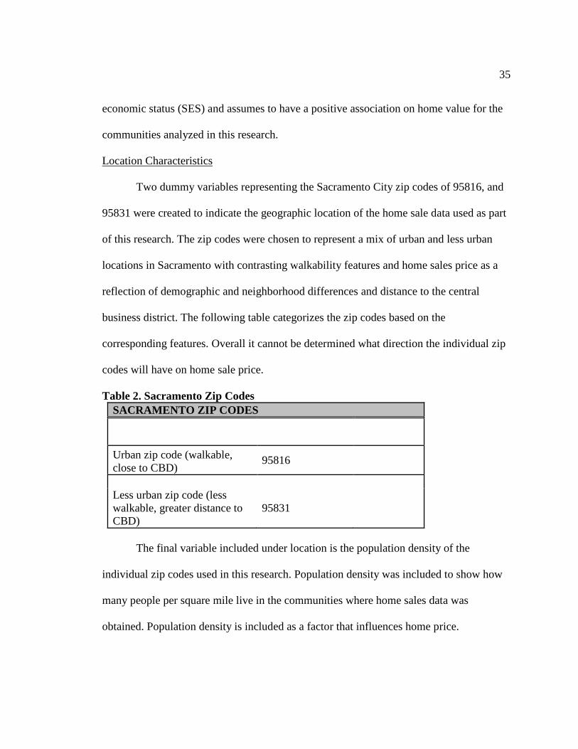
Two dummy variables representing the Sacramento City zip codes of 95816, and

95831 were created to indicate the geographic location of the home sale data used as part

of this research. The zip codes were chosen to represent a mix of urban and less urban

locations in Sacramento with contrasting walkability features and home sales price as a

reflection of demographic and neighborhood differences and distance to the central

business district. The following table categorizes the zip codes based on the

corresponding features. Overall it cannot be determined what direction the individual zip

codes will have on home sale price.

Table 2. Sacramento Zip Codes SACRAMENTO ZIP CODES

Urban zip code (walkable, close to CBD)

95816

Less urban zip code (less walkable, greater distance to CBD)

95831

The final variable included under location is the population density of the

individual zip codes used in this research. Population density was included to show how

many people per square mile live in the communities where home sales data was

obtained. Population density is included as a factor that influences home price.

36

Data Sources

I used three data sources in my research. This section provides detailed

information on the data sources and selection. A thorough understanding of the data used

in this regression model is imperative to understanding and interpreting the results.

Additional importance in providing data detail is to enable research duplication, a key

step required of sound research and policy assumptions. This chapter concludes with the

collection and organization of the data displayed in table format to allow ease of analysis.

Homes Sales Data

Home sales price in the years 2008-2009 obtained through the Multiple List Serve

(MLS) provided most of the data used in this regression analysis. The dependent variable

of home sale price or PRICE was sorted from the file to only include sales data on the

communities analyzed. The mean home sales price for the research area was $224,171

and values ranged from a very low $6053 to a high $1,550,000. Three of the six broad

independent variable categories; Home size characteristics, home structural

characteristics, and home age characteristics were exclusively obtained from the home

sales data. The mean house size in square feet was 1501 and the mean number of

bedrooms was three, mean age was slightly more than 43 years. Neighborhood

characteristics contain the two dummy variables of HOA and REO obtained from the

home sales data. Additionally, two zip code dummies were created from the home sales

data and homes sales prices were grouped by the two zip codes of 95816 and 95831.

37

Walk Score Data

The key explanatory variable is a Walkability Index as defined by Walk Score. A

total of 463 Walk Scores were obtained on home sale locations in the 95816 and 95831

zip codes. The key variable WALK provides a walkability proxy for the two zip codes.

Taken together the zip code variables represent walkability as a function of home price in

the selected areas. The rationale for the selection of the zip codes represent a desire to

analyze the effect of walkability of areas with varying degrees of home price and

neighborhood characteristics. The mean Walk Score for the research area was 51

indicating a “somewhat walkable” category, with values ranging from zero “car

dependent” to 92 “walkers paradise” (walkscore.com).

Census Data

The remaining variables used in the regression analysis were obtained from U.S.

Census data, specifically recently released (December, 2012) 5-year estimates of

American Community Survey (ACS) data for the years 2007-2011. ACS data is an

ongoing yearly survey from communities that provides statistical information used to

determine federal and state funds allocations for specific investments and services

(www.census.gov). ACS 5-year estimates are the best for analyzing very small

populations with the largest sample size. These estimates are more reliable than 1-year

and 3-year estimate released by the ACS. The geographic location analyzed from the

ACS 5-year estimates is what is known as ZCTA’s or Zip Code Tabulation Areas. Zip

Codes and Zip Code Tabulation Areas differ in that postal delivery routes use zip codes,

38

and the Census Bureau creates ZCTA’s as approximate areas corresponding the U.S.

Postal Service 5 digit zip code service areas (www.census.gov). For this regression

analysis ZCTA’s correspond most closely with the zip code areas collected for home

sales, and their use provides the latest and most reliable demographic information

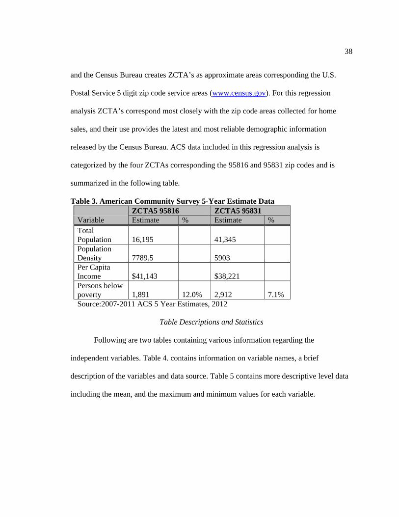
released by the Census Bureau. ACS data included in this regression analysis is

categorized by the four ZCTAs corresponding the 95816 and 95831 zip codes and is

summarized in the following table.

Table 3. American Community Survey 5-Year Estimate Data ZCTA5 95816 ZCTA5 95831 Variable Estimate % Estimate % Total Population 16,195 41,345 Population Density 7789.5 5903 Per Capita Income $41,143 $38,221 Persons below poverty 1,891 12.0% 2,912 7.1% Source:2007-2011 ACS 5 Year Estimates, 2012

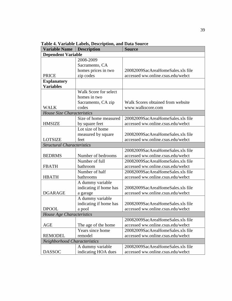
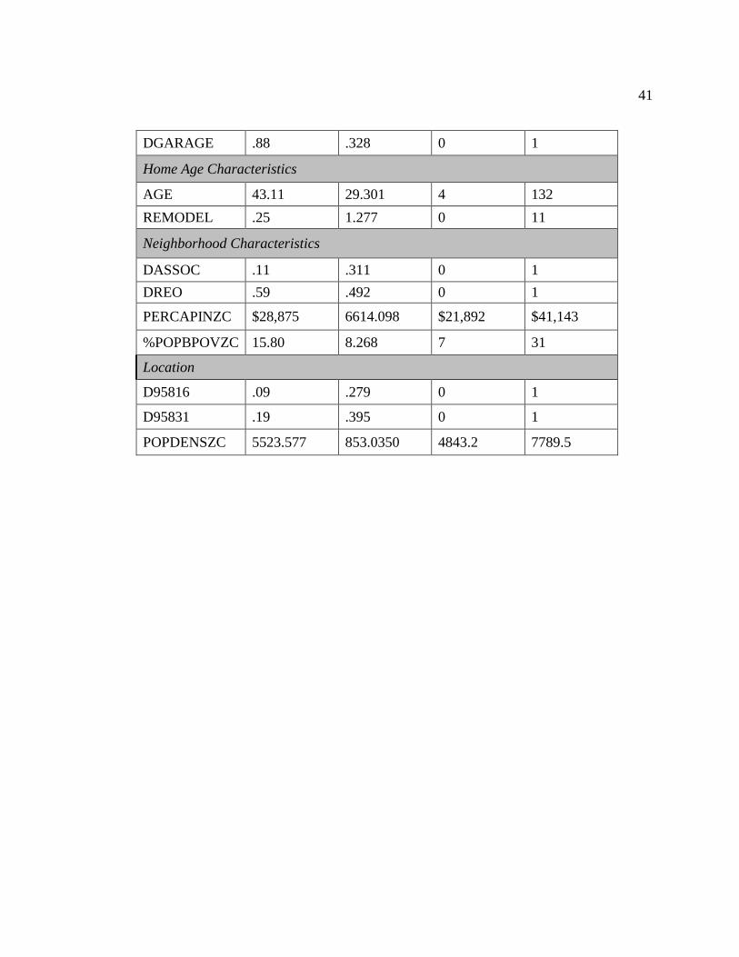
Table Descriptions and Statistics

Following are two tables containing various information regarding the

independent variables. Table 4. contains information on variable names, a brief

description of the variables and data source. Table 5 contains more descriptive level data

including the mean, and the maximum and minimum values for each variable.

39

Table 4. Variable Labels, Description, and Data Source Variable Name Description Source Dependent Variable

PRICE

2008-2009 Sacramento, CA homes prices in two zip codes

20082009SacAreaHomeSales.xls file accessed ww.online.csus.edu/webct

Explanatory Variables

WALK

Walk Score for select homes in two Sacramento, CA zip codes

Walk Scores obtained from website www.walkscore.com

House Size Characteristics

HMSIZE Size of home measured by square feet


LOTSIZE

Lot size of home measured by square feet


Structural Characteristics

BEDRMS Number of bedrooms 20082009SacAreaHomeSales.xls file accessed ww.online.csus.edu/webct

FBATH Number of full bathroom


HBATH Number of half bathrooms


DGARAGE

A dummy variable indicating if home has a garage


DPOOL

A dummy variable indicating if home has a pool


House Age Characteristics

AGE The age of the home 20082009SacAreaHomeSales.xls file accessed ww.online.csus.edu/webct

REMODEL Years since home remodel



DASSOC A dummy variable indicating HOA dues


40

DREO

A dummy variable indicating a bank owned property


PERCAPINCZC

The per capital income for a particular zip code

2007-2011 American Community Survey-Community Profile

%POPBPOVZC

The % of the adult population living in poverty by zip code


Location

D95816

A dummy variable indicating if home is located in 95816 zip code


D95831

A dummy variable indicating if home is located in 95831 zip code


POPDENZC The population density by zip code


Table 5. Descriptive Statistics

Variable Label Mean Std. Deviation Minimum Maximum

Dependent Variable PRICE $224,171 141921.042 $6,053 $1,550,000 Independent Variables WALK 51.23 16.786 0 92 Home Size Characteristics HMSIZE 1501.56 531.723 498 5583

LOTSIZE 6145.61 2789.018 0 28401

Home Structural Characteristics BEDRMS 3.08 .804 1 9 FBATH 1.84 .583 1 5 HBATH .24 .430 0 2 DPOOL .12 .328 0 1

41

DGARAGE .88 .328 0 1

Home Age Characteristics

AGE 43.11 29.301 4 132 REMODEL .25 1.277 0 11


DASSOC .11 .311 0 1 DREO .59 .492 0 1

PERCAPINZC $28,875 6614.098 $21,892 $41,143

%POPBPOVZC 15.80 8.268 7 31

Location

D95816 .09 .279 0 1

D95831 .19 .395 0 1

POPDENSZC 5523.577 853.0350 4843.2 7789.5

42

Chapter 4

FINDINGS AND INTERPRETATIONS

In the previous chapter I formulated a theoretically sound model of the regression

equation I wish to estimate. Furthermore, I have the data needed to estimate this

regression and I have anticipated the effect I expect each of the explanatory variables in

the regression model will have on home value. I offer the result of the regression analysis

in this chapter, as well as a discussion of previous findings. This chapter specifically

contains: (1) an overview of the initial regression, (2) a comparison and selection of the

ideal functional form which best represents the data, (3) the steps required to check for

errors in the equation, (4) a discussion of remedies for any such errors, and (5) an

analysis of the updated regression results. This chapter concludes with a discussion on

how the results obtained from this research compare to other findings.

Initial Regression

The basis for the rationale for initiating a regression analysis was not to make a

prediction on the relationship between Walk Score and home sales price, but rather to

determine, and then analyze, what degree, if any, the Walk Score variables had on home

sales price. From the start my research has focused on determining the impact of Walk

Score on home sales price with the objective of determining if Walk Score is a good

measure of walkability.

For a regression analysis to be valid it must adhere to certain assumptions. In part,

this chapter checks for the adherence of these assumptions. The very first assumption

being there must be a linear relationship between the dependent and key independent

43

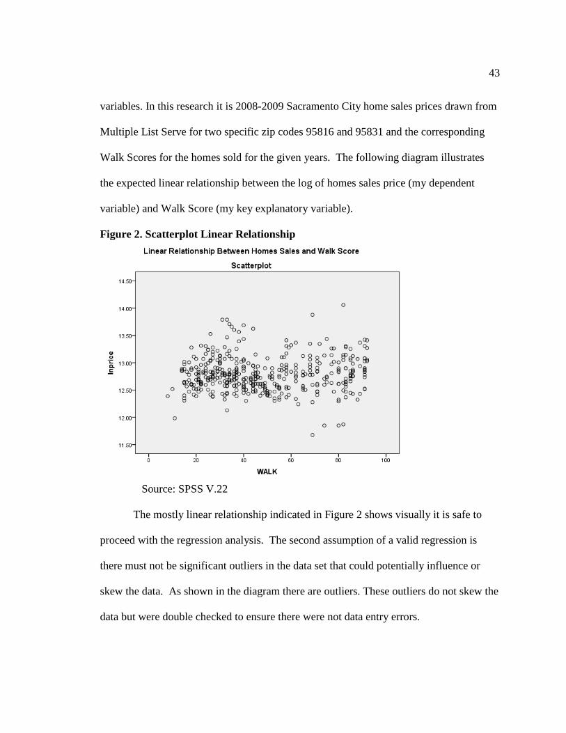
variables. In this research it is 2008-2009 Sacramento City home sales prices drawn from

Multiple List Serve for two specific zip codes 95816 and 95831 and the corresponding

Walk Scores for the homes sold for the given years. The following diagram illustrates

the expected linear relationship between the log of homes sales price (my dependent

variable) and Walk Score (my key explanatory variable).

Figure 2. Scatterplot Linear Relationship

Source: SPSS V.22

The mostly linear relationship indicated in Figure 2 shows visually it is safe to

proceed with the regression analysis. The second assumption of a valid regression is

there must not be significant outliers in the data set that could potentially influence or

skew the data. As shown in the diagram there are outliers. These outliers do not skew the

data but were double checked to ensure there were not data entry errors.

44

I conducted many different regression analyses to determine which functional

form best fit the data. The regression results recorded below represent the final result of

these tests, using various forms of some of the independent variables. It is worth noting

this at this point to validate the selection of the chosen variables. Additionally, this thesis

builds upon previous work I completed on a similar regression model. In this previous

analysis I used only data from the 95816 zip code in the Sacramento Area. In this

regression analysis I added data from the 95831 zip code which includes the Greenhaven-

Pocket area of the southern part of Sacramento, neighborhood per capita income,

population density and persons in poverty are calculated by zip code, the inclusion of the

95831 zip code dummy will need to proxy for these. The regression coefficient on the

95831 dummy variable measures the expected difference in home prices in this

neighborhood as compared to the excluded neighborhood with a zip code 95816.

The following Table 6 presents the estimated coefficients of home value as a

function of the various explanatory variables with a total of 433 observations. Table 6

includes the various functional forms of the regression analysis as well as the preferred

functional form with Variance Inflation Factors (VIFs) calculated to aide in the

evaluation of possible errors. In parenthesis are the p values for each regression

coefficient. These values must be below 0.10 for the relevant explanatory variable to

exert an influence on home on price that is statistically significant from zero. Note also

that next to each explanatory variable name in the first column of Table 6, in parentheses,

is an indication of whether the variable could be logged in one of the different regression

45

forms I tried. Additionally, and also in parentheses, the table includes the effect I

expected this variable to have on home value.

Table 6. Regression Results Comparison of Functional Form Variable Label (ln=log form)^

Log-Log Linear-Linear Log-Linear VIFs Log-Linear

CONSTANT 12.585 (.000)*

160974.819 (.000)*

12.307 (.000)*

WALKSCORE (ln) (+) .013

(.610)

-11.203 (.966)

.000 (.706) 3.809

D95831 (-) -.469 (.000)*

-166542.613 (.000)*

-.402 (.000)* 6.400

1D95816 NA NA NA NA HMSIZE (ln) (+)

.548 (.000)*

128644.119 (.000)*

.295 (.000)* 3.715

LOTSIZE (ln) (+)

.168 (.000)*

6385.367 (.000)*

.014 (.000)* 1.859

BEDROOM (ln) (-)

-.017 (.726)

-1523.112 (.791)

.001 (.928) 2.447

FULLBATH (ln) (+)

.114 (.014)*

28885.461 (.002)* .053

(.037)* 3.444

HALFBATH (+/-)

.008 (.695)

19881.888 (.825)

.010 (.628) 1.314

DPOOL (+) .033 (.135)

11249.613 (.164)

.041 (.064)* 1.143

DGARAGE (+)

.061 (.072)*

27096.482 (.029)*

.102 (.003)* 1.528

AGE (ln) (-) -.057 (.016)*

212.318 (.192)

-.001 (.250) 4.010

REMODEL (+)

.006 (.057)*

3140.454 (.008)*

.007 (.038)* 1.047

DASSOC (+) .141 (.000)*

50892.675 (.000)*

.081 (.014)* 1.396

DREO(-) -.226 (.000)*

-82945.896 (.000)*

-.227 (.000)* 1.048

R-Squared .683 .747 .682

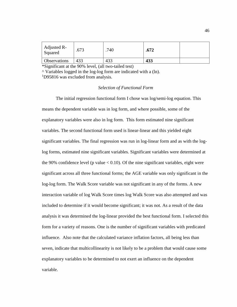
46

Adjusted R-Squared .673 .740 .672

Observations 433 433 433 *Significant at the 90% level, (all two-tailed test) ^ Variables logged in the log-log form are indicated with a (ln). 1D95816 was excluded from analysis.

Selection of Functional Form

The initial regression functional form I chose was log/semi-log equation. This

means the dependent variable was in log form, and where possible, some of the

explanatory variables were also in log form. This form estimated nine significant

variables. The second functional form used is linear-linear and this yielded eight

significant variables. The final regression was run in log-linear form and as with the log-

log forms, estimated nine significant variables. Significant variables were determined at

the 90% confidence level (p value < 0.10). Of the nine significant variables, eight were

significant across all three functional forms; the AGE variable was only significant in the

log-log form. The Walk Score variable was not significant in any of the forms. A new

interaction variable of log Walk Score times log Walk Score was also attempted and was

included to determine if it would become significant; it was not. As a result of the data

analysis it was determined the log-linear provided the best functional form. I selected this

form for a variety of reasons. One is the number of significant variables with predicated

influence. Also note that the calculated variance inflation factors, all being less than

seven, indicate that multicollinearity is not likely to be a problem that would cause some

explanatory variables to be determined to not exert an influence on the dependent

variable.

47

Also of importance, the log-linear form allows for a simple method of interpreting the

results. Specifically, the dependent variable is reflected as a percentage change as a result

of a change in the independent variables (Studenmund, 2006, p.215). Put another way, for

each independent variable, a one-unit change corresponds to a percent change in home

value. For example, the coefficient for REO is -.227 significant at the 90% level, which

means for a one-unit increase in REO, home value decreased by 22.7 percent. In addition,

a review of the histograms for the dependent and key independent variables in the various

forms log and linear, showed skewness. Specifically, the Walk Score coefficient in the

log form was negatively skewed and the linear form of the PRICE variable was positively

skewed. Using the log-linear functional form accounted for the skewness and mitigated

the effect of the final regression analysis.

The R-Squared values reported at the bottom of Table 4 above indicate the

percentage of variation in the dependent variable from the mean that is explained by the

explanatory variables. Higher R-Square values are desired due to their indication of a

“better fit” model, that is the explanatory variables more meaningfully explain the

dependent variables. However, overall fit is not the only important component of a

regression analysis. The R-Square value for the log-linear form did not yield the highest

numbers especially when compared with the linear-linear form but they are not directly

comparable across regression functional forms that take the log of the dependent variable

and do not do this. Other factors, such as the degree of fit with economic theory and

assumptions indicated by the data and model are equally, if not more important than high

R-Square values (Studenmund, 2006, p. 59).

48

Regression Analysis Errors

Ordinary Least Square (OLS) regression analysis is the model chosen for the

econometric estimation of home value as a function of various explanatory variables.

This regression analysis attempted to estimate the degree of walkability on home value in

two Sacramento zip codes. That is, OLS regression provides a sample estimate of a true

population (Studenmund, 2006, p. 37). OLS regression is the model of choice due to its

relative ease, but there are several classical assumptions that must hold for OLS to be a

preferred regression technique. Part of ensuring a valid and significant model is to

minimize and or correct for violations of assumptions. Two important assumptions that

are often violated in cross-sectional data analysis are multicollinearity and

heteroscedasticity. Multicollinearity simply means two variables are almost perfectly

linear with each other leading to problems with the regression model and

heteroskedasticity means the variance of residuals are similar to the predicted values.1

The following sections on Multicollinearity and Heteroskedasticity outline the steps taken

to reduce violations of these classical assumptions as well correcting for any errors.

Multicollinearity

Multicollinearity leads to problems of knowing which variable exerts the greatest

influence on the dependent variable. To test for multicollinearity, a two-step process was

performed on the regression model. The first step involves reviewing bivariate

correlations. An 80 percent and above threshold are a clear indication of

1 (Introduction to SAS. UCLA: Statistical Consulting Group from http://www.ats.ucla.edu/stat/sas/notes2/ accessed July 15, 2015).

49

multicollinearity. This analysis did indicate relationship values greater than 80 percent

and for this reason is what excluded from all model tests. The Census information

removed were the population density, persons below poverty, total population, and per

capita income. The second step to check for multicollinearity involves obtaining VIFs

for all the explanatory variables used in the final regression equation. The threshold for

VIFs to indicate multicollinearity is 5. VIFs greater than 5 indicate that one explanatory

variable could be explained by all other variables. It does not single out the relationship

as the bivariate correlation does, thus the need for the two-step process. As presented in

Table 4 the D95831 coefficient is the only value exceeding 5, but it was found to be

statistically significant (the problem that multicollinearity causing that it biases the

finding toward not being statistically significant) and thus there are no issues with

multicollinearity in this analysis.

Heteroskedasticity

A second classical assumption violation prevalent in cross-sectional research is

heteroskedasticity. This occurs when the variance of the error term is not constant due to

a wide variation in the values of the observed dependent variables (Studenmund, 2006,

p.348). Heteroskedasticity in of itself does not bias the coefficient estimates. However, its

presence will tend to underestimate the variance and standard errors making t-scores and

hypothesis testing unreliable. A series of steps in the regression analysis is required to

check for and correct heteroskedasticity. Prior to starting the Park Test to check for

heteroskedasticity in the equation, weighting of the variables HMSIZE and LOTSIZE

was done to control for wide variances in these observations.

50

The Park Test involves taking a final regression with the best functional form and

obtaining residuals or estimates of the error terms. Once the residuals are obtained, they

are squared then logged. The log of the square residuals is then tested in a second

regression as the dependent variable. The explanatory variable or suspected

proportionality factor Z variable is logged and is tested in the second equation as the only

independent variable. For this analysis, home size in square feet was determined to be the

Z factor due to suspected significant variation within the observations. An additional step

in the analysis finds the t-test to be statistically insignificant. The null hypothesis of

homoskedasticity may not be rejected as the absolute t-score [-1.384] is less than the

critical t-value 1.645 (10% level of significance two-tailed test, 474 degrees of freedom)

further indicating no significant conditions to correct for heteroeskedasticity.

Discussion of Findings

Model Fit

A reflection on the model is required at this point to access the quality of the

regression equation as well as discuss how well the OLS model fits the data. The R-

square value is a good starting point to begin this analysis as it is referred to as the

coefficient of determination. The R-square value provides a percentage that indicates how

well the dependent variable is explained by the regression equation. Values for R-square

range from 0 (indicating a poor fit) to 1.0, (indicating a perfect fit). The R-square value

from this research is .682 indicating 68 percent of the regression model fits or explains

home values. While this is not a relatively high value it does provide a starting point to

51

expand or change the research. It is possible that some key explanatory variables ae

missing, suggesting the existence of omitted variable bias.

Expectations and Significant Variables

As noted in the Model section of this report and presented in Table 4, most of the

variables had the expected coefficient influence. Seven variables D95831, DGARAGE,

FBATH, HMSIZE, LOTSIZE, REMODEL, DASSOC, and DREO are found to be

significant at the 90% confidence level; DPOOL was significant only in the log-linear

model. As indicated previously no interaction variables of Walk Score and zip code were

used in this research which does contrast with the prior research where a

MIDTOWNWALK coefficient was used in the final design model. These interaction

variables were not statistically significant in any form. Taking note from this prior

research it was shown this interaction variable may not be as well of an indicator of

walkability and home value in midtown Sacramento. Expanding on that this thought the

SUBURBWALK variable would also not be a good indicator of walkability and home

value in the suburban fringe of Sacramento. Prior research indicated the

MIDTOWNWALK variable should have been dropped from the equation and this study

made note of this.

New Walkability Measure

This chapter has demonstrated that although the regression analysis presented here can be

reliable and thus valid research, it is still not fully representing the value of walkable

communities. My analysis demonstrated that despite the multiple attempts to incorporate

Walk Score as an influence on home price, it was not shown to have an impact. I propose

52

using a method similar to Leinberger and Alfonzo in their evaluation of Washington D.C.

Similarly Walk Score data was obtained for neighborhoods, this data was then broken

down further to analyze micro level neighborhood characteristics that support walkability

(Leinberger and Alfonzo, 2012). In the final chapter I will review the regression model,

discuss some of its limitations and discuss why these limitations necessitated the need for

a more robust research model. Specifically, the final chapter will expand on the

walkability model I suggest can be used in conjunction with the regression analysis

presented thus far with the ultimate goal of contributing to the research agenda of

sustainable community design. It is important to keep the underlying importance of

walkability always at the forefront, to develop research that helps to support the

development of sustainable communities that are healthy, vibrant, and good for the

planet.

53

Chapter 5

AN ALTERNATIVE WALKABILITY MEASURE

As my thesis concludes, I am once again faced with answering the big questions:

Why are walkable communities important and can the current measures of walkability

truly assess the value of neighborhood sustainability?

In the first chapter of this thesis, I explained that walkable communities offer the

beginnings of creating sustainable communities. Once value is added to a place because

of the mere ability to walk from point A to point B, it can perhaps be a driver of other

sustainable features such as a more health environment and perhaps a generator of social

capital. Sustainable communities can both be economically vitality and not impose

negative external effects on other communities. The more that some communities can

adopt a model of sustainability, of which walkability is an essential part, they become a

beacon for other communities to follow.

Chapter 2 provided a brief summary of some of the relevant research on

walkability. I presented information from a health and social perspective on why creating

healthy, vibrant communities can be a way for communities to combat growing rates of

obesity from sedentary lifestyles. Creating walkable communities can be one part of

solving the problem by giving individuals the option to live in less car dependent

communities. Chapter 2 also provided the background on other research that employed

the use of Walk Score data. The relevance of Walk Score data in research was found to

be valid for some purposes and therefore had policy implications. For instance, a study

conducted using data from Louisville, Kentucky in year 2015 found Walk Score to be

54

replicable for assessing the walkability of a location and more walkable locations do

translate into higher property values, less foreclosures and less crime (Gilderbloom, et al.,

2015). An additional study from Alabama in year 2011 found Walk Score to be a good

indicator of increased land values, specifically the study found places located in the

central business district and with increased walkability did in fact increase land values

(Rauterkus & Miller, 2011). The Pivo and Fisher (2011) study of 4,200 commercial

properties around the country, from the years 2001 to 2008, employed Walk Score values

in a regression analysis concluded property values increased anywhere from 1 to 9

percent for a ten point increase in walkability based on a 100 point scale .

Chapters 3 and 4 went into more detail about my own thesis research and

methodology, as well as what specifically I was measuring and trying to convey. In

summary, I described how I will employ a regression analysis on homes sales data and

Walk Score data for Midtown and the Greenhaven-Pocket are of Sacramento with two

very different perceived walkability. The goal was to determine if walkability influenced

homes sales price, and if it did, by how much influence. The regression analysis

explained 68 percent of the real-world variation in home prices from the two chosen

Sacramento communities, but the Walk Score specifically was found to not have an

influence on home value contrary to what was expected and found in previous research.

The results of the regression analysis suggest the need for additional analysis of

the Walk Score data. The purpose of this concluding chapter will be to review the flaws

with Walk Score as evidenced in my research and to propose a method for changing it.

The remaining sections of this chapter will review Walk Score as it was used in the

55

regression and provide an explanation for why it is flawed. I will finally offer my

suggestion for developing a walkability index that addresses the Walk Score

shortcomings.

Walk Score Limitations

The concept of using a Walk Score to calculate the range of walkability for

specific residential locations is potentially a great and useful tool for consumers, realtors,

city planners, and others to use in their assessment of this trait. Alternative use in

academic research has grown in recent years with more valid data supporting its

methodology of determining the walkability of a location, but despite the merits as a

consumer housing tool and in academic research it does contain limitations that should be

addressed. My research findings indicate Walk Score data was not a significant variable

in the regression analysis, meaning Walk Scores did not have any influence on home

price. This section will review these limitations, and based on these findings, offer a

suggestion for a walkability index that takes into account the limitations.

Walk Score was found in several research studies to not account for other

walkability factors such as safety, environmental, or topographic deterrence

(Gilderbloom, et al., 2015, Pivo and & Fisher, 2011, Carr, et al., 2010). Previous research

also indicates that Walk Score can be useful to determine some walkable places, but

cannot be universally applied to measure overall neighborhood walkability (Duncan, et

al., 2011). Most important is that important factors relevant to actual walkability, such a

road routes and environmental features such as lakes or parks that determine one’s route

to a destination, are not currently accounted for. Walk Score data is also absent street

56

quality; and the algorithm does not account for trees, places to sit, sidewalk width and

overall aesthetic value of the walking route (Gildberbloom, et al., 2015, Leinberger &

Alonzo, 2012, Pivo & Fisher, 2011).

Taken as a total Walk Score is not a perfect measure of walkability. The fact is it

is a fluid data set, being updated as continued research identifies limitations. The website

www.walkscore.com includes specific information on the methodology for determining

scores and is updated as improvements are made to the algorithm. The data itself is

changing as environments change. Walk Score is a useful starting point for some

researchers, but there are other factors of walkability that should be measured when

determining community walkability.

An Alternative Walkability Measure

I propose a different method of walkability that more broadly encompasses the

health, social, and environmental benefits of a specific residential location. The current

Walk Score value calculated for a location does little to capture the broader health and

social aspects of walkability as an influence on home price. In Leinberger and Alfonso’s

(2012, p. 3) Washington D.C. study for the Brookings Institute, this lack of research was

summarized as: “…The absence of a clear classification of the mix of residential, office,

and retail elements that compromise walkable urban places or of the built environment

components (including area, density, land use characteristics, transportation facilities,

etc.) necessary to produce sustainable, economically viable, socially equitable places has

been one of most significant barriers to addressing their demand. Metrics to gauge

walkable urban places’ performance that could guide investments decisions and public

57

policy development have also been absent”. The Leinberger study initially used Walk

Score data for 201 neighborhoods and narrowed the data to include 66 places where there

were policies in place to promote walkability, mixed use development or higher densities.

This Leinberger study also focused solely on all places with Walk Scores greater than 90

which are considered a Walker’s Paradise and only a representative sampling of the other

Walk Score levels indicating most of the location sample already had a high Walk Score,

again the scale is out of 100.

To develop metrics for measuring walkability I would propose not to eliminate

those places considered car dependent or less walkable as the Leinberger and Alfonso

study did. My metrics will include all possible types of environments and include them in

any place study to highlight what makes a location a “Walker’s Paradise” and those

places not so much, so future investment can turn those places around so to speak. For

example, if the goal is to draw attention to places that capture the social, environmental,

and health aspects of walkability, a high walkability index as it is currently measured

may not be the best way to do this. There are other neighborhood features that promote

environment and health that are not in the current calculation of a Walk Score. Thus, a

different form of measure is needed.

The methodology I propose it to begin with the Walk Score (as currently

calculated) for a given location. The second step would be to conduct an audit of specific

neighborhoods whose boundaries are determined by similar Walk Scores, utilizing the

same method as the Leinberger and Alfonso (2012) study. In that study the researchers

used a 162 item Irvine Minnesota Inventory (IMI) “that collects objective data on built

58

environment characteristics hypothesized to be related to physical activity” (Leinberger

& Alfonso, 2012, p. 6). The locations were additionally assessed for ten environmental

characteristics believed to facilitate walking and which address the limitations of safety,

aesthetic walking quality, and topographic characteristics:

11. Aesthetics (attractiveness, open views, outdoor dining, maintenance)

12. Connectivity (potential barriers such as wide thoroughfares)

13. Density (building concentrations and height)

14. Form (streetscape discontinuity)

15. Pedestrian amenities (curbcuts, sidewalks, street furniture)

16. Personal safety (graffiti, litter, windows with bars)

17. Physical activity facilities (recreational uses)

18. Proximity of uses (presence of non-residential land uses)

19. Public spaces and parks (playgrounds, plazas, playing fields)

20. Traffic measures (signals, traffic calming)

Therefore, my proposed methodology includes a base line walkability index with Walk

Score data, a walkability assessment related to physical activity using the Irvine

Minnesota Inventory, and an additional assessment of the environmental characteristics

listed above, that theoretically promote walking. The final inventory is designed to

capture the social aspects of communities. The Leinberger and Alfonso (2012) study

additionally incorporated five indictors of social equity to include: income, diversity,

education, affordability, and transportation accessibility. The researchers consider social

equity metrics important to the overall walkability of a location as walkability is seen as a

59

way to increase a location’s “triple bottom line: profit (economics), people (equity), and

planet (environment)” Leinberger and Alfonso, 2012, p. 2). I would mirror these

indicators as they are easily measurable and the data sources are consistent across

metropolitan areas.

Taken together the four additional levels of indices provide a more inclusive

measure of communities that address various aspects of what actually makes a

community walkable, such as safety, community features that promote walking, and

topographic features not currently accounted for Walk Score. Incorporating this level of

assessment will help communities understand where they place in the walkability index,

where to focus resources and how to achieve an overall greater walkable community. For

instance, if one community has been identified as have higher education attainment,

higher disposable income, and higher walkability we can almost guarantee the housing

costs will inhibit racial diversity and social equality. City investment could target this

hypothetical area to promote housing affordability by way of housing subsidies or other

measures to create social diversity. Places with low walkability can implement policies to

increase density, promote infill development, and increase public transportation or other

measures to ensure future development focus on creating walkable places.

Policy Implications

The goal of this master’s thesis was to better understand the importance of

creating walkable communities and how to apply what was learned as policy actions that

communities can implement to promote more sustainable, and hence, walkable

communities. As indicated from this limited research endeavor, knowing the limitations

60

of Walk Score and accounting for the limitations and addressing them in a new

walkability index can be half the battle in implementing or promoting measures for better

designed communities. The policy implications from this are endless, from battling the

unintended health consequences of a sedentary lifestyle to preserving valuable natural

resources (think fossil fuel conservation, pollution and political unrest) to creating more

diverse and equal societies.

Community change does not happen all at once and by the mere implementation

of a policy by elected officials. It happens block by block, neighborhood by

neighborhood. It takes knowledge of what is working in a community and a clear

understanding of what needs to change. The ultimate intent of this research is for the

information presented in this thesis to actually be a useful tool to promote community

change with the goal of sustainable community design. One part of creating a sustainable

community is knowing how walkable it is because walkability ties into so many other

aspects of the health, social and environmental concerns of a community. Increased

awareness and investment in walkable communities can promote change that benefits

individuals, communities, and society as a whole.

61

References

A look at home prices and most expensive states to buy a house. (2015, May 1).

Sacramento Business Journal, 1-2. Retrieved from

http://www.bizjournals.com/sacramento/news/2015/05/01/california-median

-home-prices-expensive-states.html.

Carr, L., Dunsiger, S., and Marcus, B. (2010). Validation of Walk Score for estimating

access to walkable amenities. British Journal of Sports Medicine.

Centers for Disease Control and Prevention (2014). State indicator report on physical

activity. U.S. Department of Health and Human Services.

Cotright, J. (2009). Walking the walk: How walkability raises home values in U.S. cities.

CEOs for Cities.

Duncan, D., Aldstadt, J., Whalen, J., Melly, S., and Gortmaker, S. (2011). Validation of

Walk Score for estimating neighborhood walkability: An analysis of four US

metropolitan areas. International Journal of Environmental Research and Public

Health 8. pp. 4160-4179.

Gibbons, S. and Machin, S. (2008). Valuing school quality, better transport, and lower

crime: evidence from house prices. Oxford Review of Economic Policy 24:1, 99-

119

Giles-Corti, B., Macaulay, G., Middleton, N., Boruff, B., Bull, F., & Butterworth, I.,

Badland, H., Movao, S., Roberts, R., and Christian, H (2014). Developing a

research and practice tool to measure walkability: A demonstration project.

Health Promotion Journal of Australia, 25, 160-166.

62

Gilderbloom, J., Riggs, W., and Meares, W. (2015). Does walkability matter? An

examination of walkabilities impact on housing values, foreclosures and crime.

Cities 42, pp. 13-24.

Leinberger, C. and Alfonso, M. (2012). Walk this way: The economic promise of

walkable places in metropolitan Washington D. C. Metropolitan Policy Program

at Brookings.

Leyden, K.M. (2003). Social capital and the built environment: the importance of

walkable neighborhoods. American Journal of Public Health 93 (9), 1546-1551.

Litman, T. (2007). Economic value of walkability. Victoria Transport Policy Institute,

pp. 1-24.

Lovasi, G., Grady, S., and Rundle, A. (2012). Steps forward: Review and

recommendations for research on walkability, physical activity and cardiovascular

health. Public Health Review 33, pp. 484-506.

Matthews, J.W. and Turnbull G.K. (2007), ―Neighborhood street layout and property

value: the interaction of accessibility and land use mix. Journal of Real Estate

Finance and Economics 35, pp. 111-141.

National Association of REALTORS (2010). On common ground; Green communities.

Winter 2010.

Pivo, G. and Fisher, J. (2011). The walkability premium in commercial real estate

investments. Real Estate Economics V, pp.1-35.

Rosen, S. (1974). Hedonic prices and implicit markets: Product differentiation in pure

competitions. Journal of Political Economy, 82, 1, 34-55.

63

Sallis, J., Spoon, C., Cavill, N., Engelberg, J., Gebel, K., Parker, M., Thronton, C., Lou,

D., Wilson, A., Cutter, C., and Ding, D. (2015). Co-benefits of designing

communities for active living; an exploration of the literature. International

Journal of Behavioral Nutrition and Physical Activity 12.

Schwartz, A., et al. (2003). Has falling crime driven New York City’s real estate boom?

Journal of Housing Research., 14 (1), 101–136

Shultz, S.D. and King, D.A. (2001). The use of Census Data for hedonic price estimates

of open-space amenities and land use. Journal of Real Estate Finance and

Economics 22, 2, 239-252

Song, Y., and Knaap, G. J. (2004). Measuring the effects of mixed land uses on housing

values. Regional Science and Urban Economics, 34, 6, 663–680

Studenmund, A.H. (2006). Using econometrics: A practical guide. Pearson Educational,

Inc. Boston, MA.

Walk Score methodology. Retrieved from

https://www.walkscore.com/methodology.shtml.

Tu, C.C. and Eppli, M.J. (2001). An empirical examination of traditional neighborhood

development. Real Estate Economics 29 (3), 485-501.

Documents

VALUE OF WALKABLE COMMUNITIES A Thesis … Thesis Presented to the faculty of the Department of Public Policy and Administration California State University, Sacramento Submitted in