Embed Size (px)
Citation preview
Valuation of Structured Financial Products
by Adaptive Multiwavelet Methods
in High Dimensions
Rüdiger Kiesel, Andreas Rupp und Karsten Urban
Preprint Series: 2013 - 10
Fakultät für Mathematik und Wirtschaftswissenschaften
UNIVERSITÄT ULM
VALUATION OF STRUCTURED FINANCIAL PRODUCTS BY
ADAPTIVE MULTIWAVELET METHODS IN HIGH
DIMENSIONS
RUDIGER KIESEL, ANDREAS RUPP, AND KARSTEN URBAN
Abstract. We introduce a new numerical approach to value structured finan-cial products.
These financial products typically feature a large number of underlying as-
sets and require the explicit modelling of the dependence structure of theseassets. We follow the approach of Kraft and Steffensen (2006,[26]), who ex-
plicitly describe the possible value combinations of the assets via a Markov
chain with a portfolio state space.As the number of states increases exponentially with the number of assets
in the portfolio, this model so far has been – despite its theoretical appeal –
not computational tractable.The price of a structured financial product in this model is determined by
a coupled system of parabolic PDEs, describing the value of the portfolio foreach state of the Markov chain depending on the time and macroeconomic state
variables. A typical portfolio of n assets leads to a system of N = 2n coupled
parabolic partial differential equations. It is shown that this high number ofPDEs can be solved by combining an adaptive multiwavelet method with the
Hierarchical Tucker Format. We present numerical results for n = 128.
1. Introduction
The inadequate pricing of Asset-backed securities (ABS) and in particular Col-lateralized Debt Obligations (CDOs), on which we focus, is widely viewed as a maintrigger of the financial crisis that started in 2007, [6, 17].
The lack of adequate mathematical models to capture the (dependency) riskstructure, [23], of these assets is consistently identified as the main reason for theinaccurate pricing. Due to the complexity of a CDO portfolio, which arises fromthe high number of possible default combinations, drastic simplifications of theunderlying portfolio structure had to be made in order to compute a price, [7, 9, 43].
We consider the CDO model of [26] where the value of a CDO portfolio is deter-mined by a system of coupled parabolic PDEs, each PDE describing the portfoliovalue for a specific default situation. These default situations are characterizedby a discrete Markov chain, where each state in the Markov chain stands for adefault state of the portfolio. Therefore, for a portfolio of n assets, there areN = 2n possible combinations of defaults and, therefore, 2n states in the Markovchain. It will later turn out to be convenient to label the states in the index setN ∶= 0, . . . ,N − 1. The value of the CDO portfolio in [26] is described by thefunction u(t, y) = (u0(t, y), . . . , uN−1(t, y))T that satisfies the partial differentialequation for all t ∈ (0, T ) (T > 0 being the maturity) and all y ∈ Ω ⊂ RM . The yvariables are used to incorporate M economic market factors which describe the
1
2 RUDIGER KIESEL, ANDREAS RUPP, AND KARSTEN URBAN
state of the economy.
ujt(t, y) = −1
2∇ ⋅ (B(t)∇uj(t, y)) −αT (t)∇uj(t, y) + r(t, y)uj(t, y)
− ∑k∈N∖j
qj,k(t, y)(aj,k(t, y) + uk(t, y) − uj(t, y)) − cj(t, y),(1.1a)
u(t, y) = 0, t ∈ (0, T ), y ∈ ∂Ω,(1.1b)
u(T, y) = (u0T (y), . . . , u
N−1T (y))T , y ∈ Ω,(1.1c)
for all j ∈ N . The differential operator ∇ is to be understood w.r.t. the variabley. Often the bounded domain Ω arises from localizing the problem from RM to abounded domain by truncation.
This is a generalized Black-Scholes PDEs with a linear coupling, homogeneousDirichlet boundary conditions (1.1b) in y (possibly after localization) and terminalcondition (1.1c). The remaining parameters can be interpreted as follows:
The space variables y ∈ Ω ⊂ RM describe the current market situation bymeans of variables which describe the market influence on the CDO port-folio. This could be for example interest rates, foreign exchange rates,macroeconomic factors and other factors depending on the composition ofthe portfolio. These space variables are modelled via a market processdY (t) = α(t)dt + β(t)dW (t), where W (t) is a M -dimensional standardBrownian motion, the drift α(t) is a M -dimensional vector and the volatil-ity β(t) ∈ RM×M . Then, we abbreviate B(t) ∶= β(t)β(t)T . By normaliza-tion, we may assume w.l.o.g. Ω = [0,1]M .
N is the state space of a Markov chain, where each state is a possiblecombination of defaults of the underlying portfolio.
The function r(t, y) describes the relevant market interest rate.
The parameters qj,k ≥ 0 are the transition intensities, which is the instan-taneous change in the transition probabilities, from state j into state k,where j, k ∈ N . Moreover, for any state j, all intensities sum up to zero,i.e., qj,j ∶= −∑k∈N∖j q
j,k. The default probability is assumed to increaseover time, see [26].
The payments cj(t, y), j ∈ N , made by the CDO are assumed to be contin-uous in time.
The recovery payment, i.e., the distribution of the remaining funds of thedefaulted firm, is denoted by aj,k(t, y). It depends on the transition fromstate j to state k, which means on the defaulted firm.
Final payments at maturity can also be included. They also depend on thestate and the current market situation and are denoted by ujT (y).
All together, (1.1) is a system of N = 2n coupled time-dependent parabolic PDEseach in dimension M . The difficulty of this pricing approach is primarily the highnumber N = 2n of states in the Markov chain and, hence, the high number ofcoupled partial differential equations. In the following it will be shown, that underreasonable conditions, the high dimensionality resulting from the Markov chain canbe separated as a time dependent factor from the actual solution of the partial dif-ferential equation. This allows to represent the system of coupled partial differentialequations in variational form as the variational formulation of a high dimensionalparabolic partial differential equation. We propose to use orthogonal multiwavelet
ADAPTIVE MULTIWAVELET METHODS FOR STRUCTURED FINANCIAL PRODUCTS 3
bases to develop an equivalent discrete but infinite-dimensional system. This par-ticular choice allows to write the system as a tensor product, which in turns leadsto decoupling the Markov chain ingredients from the market parameters, i.e., thehigh dimensionality is separated from the integrals of the test and trial spaces.The hierarchical Tucker Format (HTF), is then applied to this tensor structure.To numerically approximate a solution for this system, multiwavelets ensure smallcondition numbers regardless of the dimension of the process. Moreover, this choiceallows for asymptotically optimal adaptive schemes, see e.g. [24].
In the context of wavelet approximations of solutions of partial differential equa-tions, the term “high dimensional” commonly refers to the dimension M of thespace variable, say M ≥ 5. In our problem at hand, we also have a huge numberN = 2n of coupled equations. As already mentioned, we will show that we canseparate both ingredients, namely the Markov chain state space N and the macro-economic model Ω ⊆ RM . The latter one will be discretized by a tensor productmultiwavelet bases. In general, the dimension of the basis grows exponentially withM – the curse of dimensionality. Thus, the number of macroeconomic variablesthat can be used is often strongly limited by the available memory. This can beseen in [13], where the number of degrees of freedom in 10 dimensions is not enoughto reach the optimal convergence rate. In [34] it can also be seen, that the numberof degrees of freedom which can be used in 5 dimensions is strongly limited. By ap-plying principal component analysis, [35], the authors are able to solve a problem in30 dimensions essentially by a reduction to 5 dimensions. In [22], 8 dimensions arereached for a full rank Black Scholes model and 16 dimensions, when a stochasticvolatility model is considered.
The remainder of this paper is organized as follows. In Section 2, we derive avariational formulation to (1.1) and prove its well-posedness. Section 3 is devotedto the description of well-known multiwavelet bases and the collection of the mainproperties that are needed here. The discretization in Section 4 is done in threesteps. First, we use the multiwavelet basis in order to derive an equivalent discretebut infinite-dimensional system. We also show that this approach allows to decouplethe market variables from the Markov chain state space in terms of a tensor product.The next two steps involve the discretization in time and market variables. Dueto the mentioned separation, we can handle large portfolios of companies by theso-called Hierarchical Tucker Format (HTF) which is briefly reviewed in Section 5concentrating on those properties that are relevant here. Finally, in Section 6, wereport on some numerical experiments for realistic market scenarios. We collectsome auxiliary facts in Appendix A.
2. Variational formulation
We start by deriving a variational formulation of the original system (1.1). Westart with some remarks on systems of elliptic partial differential equations. LetV H V ′ be a Gelfand triple and V ∶= V N be the tensor product space. Foru = (u0, . . . , uN−1)T , v = (v0, . . . , vN−1)T ∈ V, let aj ∶ V × V → R be a multilinearform and f j ∶ V → R, j = 0, . . . ,N − 1, a linear form. Then,
(2.1) u ∈ V ∶ aj(u, v) = f j(v) ∀ v ∈ V, j ∈ N ,
4 RUDIGER KIESEL, ANDREAS RUPP, AND KARSTEN URBAN
is a coupled linear system of N equations. Defining a ∶ V ×V → R, f ∶ V → R we
a(u,v) ∶= ∑j∈N
aj(u, vj), f(v) ∶= ∑j∈N
f j(vj), u,v ∈ V,
obtain a variational problem
(2.2) u ∈ V ∶ a(u,v) = f(v) ∀v ∈ V,
which is well-posed provided the well-known Necas conditions are valid, [32]. Notethat (2.1) and (2.2) are equivalent since using the test functions vjδj , whereδj = (δj,j′)
Tj′∈N (δi,j denoting the Kronecker delta) in (2.2) yields (2.1); the other
direction is trivial.Next, we need to separate the high dimensional Markov chain parts from the
variational formulation. This means that the state dependent variables are com-pound functions of a state dependent part (which might also depend on the timet) and a mutual factor depending on the space variables y. Hence, we assumethat there exist functions qj,k, aj,k, cj ∶ [0, T ] → R, constants aj ∈ R and functionshq, ha, hc, ha(T ) ∶ Ω→ R such that
qj,k(t, y) = qj,k(t)hq(y), aj,k(t, y) = aj,k(t)ha(y),(2.3a)
cj(t, y) = cj(t)hc(y), aj(y) = aj ha(T )(y),(2.3b)
for all j, k ∈ N , t ∈ [0, T ] and y ∈ Ω. This is a reasonable assumption from thefinancial point of view since it states that the dependency on the market processis the same for all points in time and for all states in the Markov chain. The fact,that changes of the state of the Markov chain cannot alter the dependency of themarket process Y means that default of single firms in the CDO portfolio will notchange the market situation. Finally, we remark that there are methods availablein order to obtain an approximate representation of the form (2.3) even in caseswhere the functions do not directly allow such a separation of variables, see e.g.[4, 33].
We are now going to derive a variational formulation. We need one more ab-breviation: If v ∶ (0, T ) × Ω → R is a function in time and space, we will alwaysabbreviate v(t) ∶ Ω→ R, where v(t)(y) ∶= v(t, y), y ∈ Ω.
Definition 2.1. Given assumption (2.3), a function u ∈ X ∶= L2(0, T ;H10(Ω)N) ∩
H1(0, T ;H−1(Ω)N) is called weak solution of (1.1) if
(2.4) (ut(t),v)0;Ω + a(u(t),v) = (f(t),v)0;Ω for all v ∈H1
0(Ω)N , t ∈ [0, T ]
u(T, y) = uT (y) ∶= (u0T (y), . . . , u
N−1T (y))T
where (w,v)0;Ω = ∑j∈N (wj , vj)0;Ω, a(w,v) ∶= ∑j∈N aj(w, vj) with
aj(w(t), v) ∶=1
2(∇wj(t),B(t)∇v)0;Ω − (α(t)T∇wj(t) + γj(t)Tw(t), v)0;Ω(2.5)
the reaction coefficient (j, k ∈ N )
γjk(t, y) ∶= (γj(t, y))k ∶=
⎧⎪⎪⎨⎪⎪⎩
−qj,k(t)hq(y) if k /= j,
r(t) −∑k′∈N∖j qj,k′(t)hq(y) if k = j.
and the right-hand side (f(t),v)0;Ω ∶= ∑j∈N (f j(t), vj)0;Ω with f j(t) ∶= −cj(t)hc(y)−
∑k∈N∖j qj,k(t) aj,k(t)ha(y)hq(y).

ADAPTIVE MULTIWAVELET METHODS FOR STRUCTURED FINANCIAL PRODUCTS 5
Obviously, (2.4) is a system of instationary convection-diffusion-reaction equa-tion and the linear coupling is in the zero-order (reactive) term.
Theorem 2.2. Let (2.3) hold. If u ∈ C1([0, T ]; (C2(Ω))N) is a classical solutionof (1.1), then it is also a weak solution in the sense of Definition 2.1. On the otherhand, if u is a weak solution and additionally u ∈ C1([0, T ]; (C2(Ω))N), then u isalso a classical solution of (1.1).
Proof. We multiply (1.1) with some vj ∈H10(Ω) and obtain
(ujt(t), vj)0;Ω = (r(t)uj(t), vj)0;Ω − (α(t)T∇uj(t), vj)0;Ω
−1
2(∇ ⋅ (B(t)∇uj(t)), vj)0;Ω
− ∑k∈N∖j
∫Ωqj,k(t, y) (uk(t, y) − uj(t, y))vj(y)dy
−∫Ωcj(t, y) + ∑
k∈N∖jqj,k(t, y)aj,k(t, y)vj(y)dy.
Using assumption (2.3), the (negative of the) last term reads
cj(t)∫Ωhc(y) v
j(y)dy +∑
k∈N∖jqj,k(t) aj,k(t)∫
Ωhq(y)ha(y) v
j(y)dy = (f j(t), vj)0;Ω.
Integration by parts gives for the last term
1
2(B(t)∇uj(t)),∇vj)0;Ω − (α(t)T∇uj(t), vj)0;Ω(2.6)
+∫Ωr(t)uj(t, y) − ∑
k∈N∖jqj,k(t)hq(y)(u
k(t, y) − uj(t, y))vj(y)dy,
where the last term is equal to (γj(t)Tu(t), vj)0;Ω. Summing over j ∈ N yields(2.4). The above derivation also proves the claim.
The next step is to prove well-posedness of the variational problem.
Theorem 2.3. If B(t) has rank M , then (2.4) is well-posed.
Proof. We need to show that the bilinear form a(⋅, ⋅) satisfies the Garding inequalityand is continuous. Then, the claim follows from the Lax-Milgram theorem.
Remark 2.4. Note that (2.3) is not needed for the well-posedness of (2.4).
Finally, consider a space-time variational formulation of (2.4) by integrating overtime. With
b(u,v) ∶= ∫
T
0[(ut(t),v1)0;Ω + a(u(t),v1)]dt + (u(T ),v2)0;Ω
f(v) ∶= ∫
T
0(f(t),v1(t))0;Ω + (uT ,v2)0;Ω
for u ∈ X and v ∈ Y ∶= L2(0, T ;H10(Ω)N)×L2(Ω)N , v = (v1,v2) ∈ Y, the space-time
variational formulation reads
(2.7) u ∈ X ∶ b(u,v) = f(v) ∀v ∈ Y.
This latter problem is also well-posed following the arguments e.g. in [38, 46].
6 RUDIGER KIESEL, ANDREAS RUPP, AND KARSTEN URBAN
3. Multiwavelets
Since we want to use multiwavelets for the discretization of the macroeconomicvariables, we briefly recall some facts of these function systems. A (standard, notmulti-) wavelet system is a Riesz basis Ψ ∶= ψλ ∶ λ ∈ J of L2(Ω), where λ = (`, k),∣λ∣ ∶= ` ≥ 0 denotes the level (also steering the size of the support in the sense that
diam(supp ψλ) ∼ 2−∣λ∣) and k indicates the position of supp ψλ, e.g. the center ofthe support. Wavelets are (among other parameters) characterized by a certainorder d of vanishing moments, i.e.,
(3.1) ∫Ωyr ψλ(y)dy = 0 ∀0 ≤ ∣r∣ ≤ d − 1 ∀λ ∈ J , ∣λ∣ > 0.
This means that wavelets necessarily oscillate which also explains the name. Notethat (3.1) only holds for ∣λ∣ > 0. Those functions ψλ with ∣λ∣ = 0 are not wavelets butso-called scaling functions and those are generated by a single so-called generatorϕ ∈ C0(Ω) in the sense that each ψλ, ∣λ∣ = 0, is a linear combination of (possibly toΩ restricted) shifts ϕ(⋅ −k), k ∈ Z. The wavelets ψλ, ∣λ∣ > 0, are linear combinationsof dilated versions of scaling functions.
The difference of multiwavelets as opposed to wavelets is that linear combinationsof shifts of several generators ϕi, i = 1, . . . ,m, are allowed. The main advantage isthat corresponding multiwavelets may be constructed that are
piecewise polynomial, L2-orthogonal, compactly supported with small support size.
These three properties are quite useful for numercial methods since they allowan efficient evaluation of an approximation as well as well-conditioned and sparsesystem matrices.
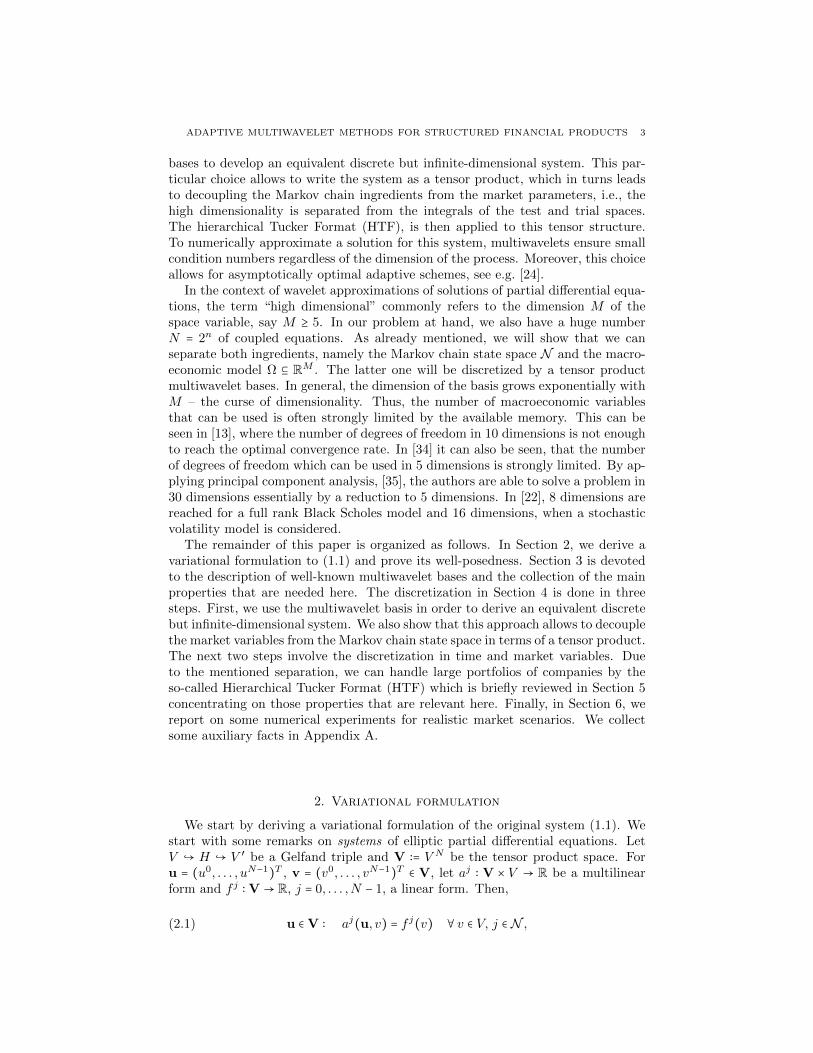
We use B-spline multiple generators and wavelets as constructed in [16, 19].These functions are also adapted to finite intervals and allow for homogeneousDirichlet boundary conditions, the latter construction was introduced in [36]. Wefaced some difficulties with the realization of the construction in [16] in partic-ular for higher regularity. However, we finally came up with a realization usingMathematica® for almost arbitrary regularity. Some functions are shown in Fig-ures 1 and 2. Details can be found in [36].
0.2 0.4 0.6 0.8 1.0x
-2
-1
1
2
3
yY1
0.2 0.4 0.6 0.8 1.0x
-2
-1
1
2
3
yY2
-1.0 -0.5 0.5 1.0x
-2
-1
1
2
3
yY3
-1.0 -0.5 0.5 1.0x
-2
-1
1
2
3
yY4
-1.0 -0.5 0.5 1.0x
-2
-1
1
2
3
yY5
-1.0 -0.5 0.5 1.0x
-2
-1
1
2
3
yY6
Figure 1: Wavelets generated by the piecewise cubic MRA having one continuousderivative.
ADAPTIVE MULTIWAVELET METHODS FOR STRUCTURED FINANCIAL PRODUCTS 7
0.2 0.4 0.6 0.8 1.0x
-2
-1
1
2
3
yHYleftL1
0.2 0.4 0.6 0.8 1.0x
-2
-1
1
2
3
yHYleftL2
0.2 0.4 0.6 0.8 1.0x
-3
-2
-1
1
2
3
yIYrightM1
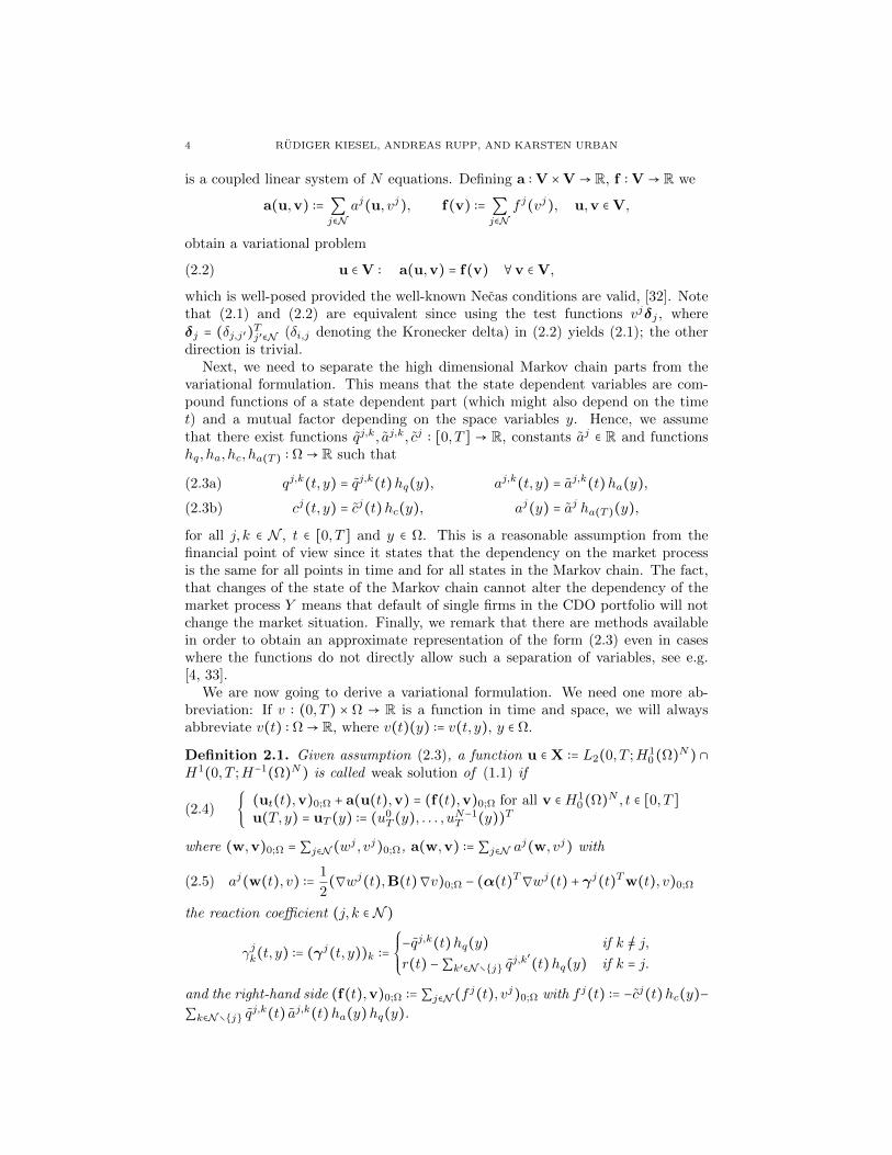
Figure 2: Wavelets with homogeneous Dirichlet boundary conditions generated bya piecewise cubic MRA on [0,1] with one continuous derivative.
Let us summarize some properties that we will need in the sequel.
Proposition 3.1 ([16]). Let Ψ = ψλ ∶ λ ∈ J be a system of multiwavelets onΩ = [0,1] from [16] normalized in H1(Ω), i.e., ∥ψλ∥1;Ω ∼ 1. Then,
(a) Ψ is L2-orthogonal, i.e., (ψλ, ψµ)0;Ω = δλ,µ∥ψλ∥20;Ω, λ,µ ∈ J ;
(b) ψλ ∈H10(Ω), λ ∈ J ;
(c) The system Ψ is a Riesz basis for H10(Ω) with L2-orthogonal functions.
Finally, denoting J ∶= (j, λ) ∶ j ∈ N ;λ ∈ J = N × J (i.e., ∣J ∣ = N ∣J ∣),λ ∶= (j, λ) ∈ J and ψλ ∶= ψλδj , λ = (j, λ) ∈ J , the system Ψ ∶= ψλ ∶ λ ∈ J is atensor product Riesz basis for H1
0(Ω)N .
4. Discretization
4.1. An equivalent `2-problem. The first step towards an adaptive multiwaveletmethod is to rewrite the variational problem (2.4) and (2.7) in a discrete equivalentproblem on the sequence space `2(J ) for the multiwavelet expansion coefficients.It turns out that the assumption (2.3) is particularly useful here, since it allows fora separation of state and space (and time), so that the discrete operators are oftensor product form. This also allows for an efficient numercial realization, also forthe space-time variational formulation [25] and in particular for larger M .
Using Ψ as defined in Section 3, the solution u of (2.4) has a unique expansionof the form
u(t, y) = ∑λ∈J
xλ(t)ψλ(y), t ∈ (0, T ), y ∈ Ω,
where xλ(t) = xjλ(t), λ = (j, λ), xj(t) = (xjλ(t))λ∈J ∈ `2(J ). The above sum is to
be understood componentwise, i.e., uj(t, y) = ∑λ∈J xjλ(t)ψλ(y) for j ∈ N . Then,
for λ = (j, λ) ∈ J , we get
aj(u(t), ψλ) = ∑µ∈J
xµ(t)1
2(∇ψµ,B(t)∇ψλ)0;Ω − (α(t)T ∇ψµ, ψλ)0;Ω
+ ∑k∈N
(γjk(t)uk(t), ψλ)0;Ω.
Defining A(t) ∶= ( 12(∇ψµ,B(t)∇ψλ)0;Ω − (α(t)T ∇ψµ, ψλ)0;Ω)
λ,µ∈J, the first sum
can be abbreviated as A(t)xj(t). The remaining term can be further detailed as
∑k∈N
(γjk(t)uk(t), ψλ)0;Ω = ∑
k∈N∑µ∈J
xkµ(t)(γjk(t)ψµ, ψλ)0;Ω = [ ∑
k∈NCj,k
(t)xk(t)]λ,
8 RUDIGER KIESEL, ANDREAS RUPP, AND KARSTEN URBAN
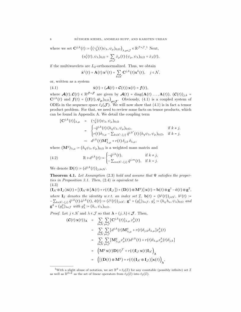
where we set Cj,k(t) ∶= ((γjk(t)ψλ, ψµ)0;Ω)λ,µ∈J ∈ RJ×J .1 Next,
(ujt(t), ψλ)0;Ω = ∑µ∈J
xµ(t) (ψµ, ψλ)0;Ω = xλ(t),
if the multiwavelets are L2-orthonormalized. Thus, we obtain
xj(t) +A(t)xj(t) + ∑k∈N
Cj,k(t)xk(t), j ∈ N ,
or, written as a system
(4.1) x(t) + (A(t) + C(t))x(t) = f(t),
where A(t),C(t) ∈ RJ×J are given by A(t) = diag(A(t) . . . ,A(t)), (C(t))j,k =
Cj,k(t) and f(t) = ((f(t),ψµ)0;Ω)µ∈J . Obviously, (4.1) is a coupled system of
ODEs in the sequence space `2(J ). We will now show that (4.1) is in fact a tensorproduct problem. For that, we need to review some facts on tensor products, whichcan be found in Appendix A. We detail the coupling term
[Cj,k(t)]λ,µ = (γjk(t)ψλ, ψµ)0;Ω
=
⎧⎪⎪⎨⎪⎪⎩
−qj,k(t) (hqψλ, ψµ)0;Ω, if k ≠ j,
r(t)δλ,µ −∑k∈N∖j qj,k′(t) (hqψλ, ψµ)0;Ω, if k = j,
=∶ dj,k(t)Mqλ,µ + r(t) δj,k δλ,µ,
where (Mq)λ,µ ∶= (hqψλ, ψµ)0;Ω is a weighted mass matrix and
(4.2) R ∋ dj,k(t) ∶=
⎧⎪⎪⎨⎪⎪⎩
−qj,k(t), if k ≠ j,
−∑m∈N∖j qj,m(t), if k = j.
We denote D(t) ∶= (dj,k(t))j,k∈N .
Theorem 4.1. Let Assumption (2.3) hold and assume that Ψ satisfies the proper-ties in Proposition 3.1. Then, (2.4) is equivalent to(4.3)(IN ⊗ IJ )x(t)+ [(IN ⊗ [A(t)+ r(t)IJ ])+ (D(t)⊗Mq
)]x(t) = b(t)⊗g1− c(t)⊗g2,
where II denotes the identity w.r.t. an index set I, b(t) = (bj(t))j∈N , bj(t) ∶=
−∑k∈N∖j qj,k(t) aj,k(t), c(t) ∶= (cj(t))j∈N , g1 = (g1
λ)λ∈J , g1λ ∶= (hq ha, ψλ)0;Ω and
g2 = (g2λ)λ∈J with g2
λ ∶= (hc, ψλ)0;Ω.
Proof. Let j ∈ N and λ ∈ J so that λ = (j, λ) ∈ J . Then,
(C(t)x(t))λ = ∑k∈N
∑µ∈J
[Cj,k(t)]λ,µ x
kµ(t)
= ∑k∈N
∑µ∈J
[dj,k(t)Mqλ,µ + r(t)δj,kδλ,µ]x
kµ(t)
= ∑k∈N
∑µ∈J
[Mqλ,µx
kµ(t)d
j,k(t) + r(t)δλ,µx
kµ(t)δj,k]
= (Mq x(t)D(t)T + r(t)IJ x(t)IN )λ
= ([(D(t)⊗Mq) + r(t)(IN ⊗ IJ )]x(t))
λ,
1With a slight abuse of notation, we set RI = `2(I) for any countable (possibly infinite) set Ias well as RI×I as the set of linear operators from `2(I) into `2(I).
ADAPTIVE MULTIWAVELET METHODS FOR STRUCTURED FINANCIAL PRODUCTS 9
where we have used Lemma A.4 in the last step. Note that D(t) ∈ RN×N , Mq ∈
RJ×J , thus (D(t)⊗Mq) ∈ R(N×J )×(N×J ) = RJ×J . Finally, we consider the right-hand side. We obtain
(b(t)⊗ g1− c(t)⊗ g2
)(j,λ)= bj(t) g1λ − c
j(t) g2
λ
= −∑k∈N∖j
qj,k(t) aj,k(t) (hq ha, ψλ)0;Ω − cj(t) (hc, ψλ)0;Ω
= (f j(t), ψλ)0;Ω,
so that the claim is proven.
4.2. Temporal discretization. So far (4.3) is equivalent to the original PDE. Asa first step towards a (finite) discretization, we consider the time interval [0, T ],fix some K ∈ N and set ∆t ∶= 1
Kas well as tk ∶= k∆t, k = 0, . . . ,K. Obviously,
(4.3) takes the form M x(t) +A (t)x(t) = f(t), x(T ) = xT , to which we apply thestandard θ-scheme (θ ∈ [0,1]) to derive an approximation xk ≈ x(tk) by solving
xK = xT ,1
∆tM (xk+1
− xk) + θA (tk+1)xk+1
+ (1 − θ)A (tk)xk = θf(tk+1) + (1 − θ)f(tk),
for k = K − 1, . . . ,0. Obviously, the second equation amounts solving the followinglinear system in each time step
(4.4) (M +∆t(θ−1)A (tk))xk = (M +∆t θA (tk+1))xk+1
+θf(tk+1)+ (1−θ)f(tk).
4.3. Wavelet Galerkin methods. The last step towards a fully discrete systemsin space and time is the discretization with respect to the economic variable y ∈ Ω.After having transformed (2.4) into the discrete but infinite-dimensional system(4.3), this can easily be done by selecting a finite index set Λ ⊂ J . Hence, weobtain
MΛ ∶= IN ⊗ IΛ, AΛ(t) ∶= IN ⊗ [AΛ(t) + r(t)IΛ] +D(t)⊗MqΛ,
which is then inserted into (4.4) for M and A (t), respectively, in order to get afinite system. We denote by AΛ(t) ∶= A(t)∣Λ = (aλ,µ(t))λ,µ∈Λ the restriction of theoriginal bi-infinite operator A(t) to a finite index set Λ ⊂ J , ∣Λ∣ <∞ (and similarlyIΛ, Mq
Λ). The choice of Λ is done in an adaptive manner, i.e., we get a sequence
Λ(0) → Λ(1) → Λ(2) → ⋯ by one of the known adaptive wavelet schemes that havebeen proven to be asymptotically optimal, [11, 10, 12, 24, 37, 45].
5. The Hierarchical Tucker Format (HTF)
In this section, we briefly recall the main properties of the Hierarchical TuckerFormat (HTF) and describe key features of our implementation. We concentrateon those issues needed for the pricing problem under consideration and refer e.g.to [20, 21, 27, 36] for more details.
We call w ∈ RK, K = ⨉j∈N Kj with entries wi ∈ R, i = (i0, . . . , iN−1)T = (ij)j∈N ,
ij ∈ Kj , a tensor of order N .2 Note that we will consider the cases Kj = Ij (a vector-tensor) as well as Kj = Jj × Ij (a matrix-tensor), where Ij and Jj are suitable(possibly adaptively chosen) index sets. Storing and numerically manipulatingtensors exactly is extremely expensive since the amount of storage and work grows
2The indexation here is adapted to our problem at hand and thus differs from the standard
literature on the Hierarchical Tucker Format.
10 RUDIGER KIESEL, ANDREAS RUPP, AND KARSTEN URBAN
exponentially with the order. Hence, one wishes to approximate a tensor w (orvec(w), which denotes the vector storage of w using reverse lexicographical orderw.r.t. the indices) by some efficient format. One example is the Tucker Format,[44], where one aims at determining an approximation
(5.1) vec(w) ≈ V vec(c) = (VN−1 ⊗⋯⊗ V0) vec(c), Vj ∈ RIj×Jj , j ∈ N ,
with the so called core tensor c ∈ RJ , J = ⨉j∈N Jj . It is known that the High-Order Singular Value Decomposition (HOSVD) (see (5.2) below) yields a ‘nearly’optimal solution to the approximation problem (5.1) which is also easily numericallyrealizable, [36]. However, the storage amount for the core tensor c still growsexponentially with N . This is the reason to consider alternative formats such asthe HTF which provides an efficient multilevel format for the core tensor c. In orderto be able to describe the HTF, it is useful to introduce the concept of matricizationas well as to describe the HOSVD in some more detail.
The direction indices 0, . . . ,N − 1 of a tensor w ∈ RI are also called modes.Consider a splitting of the set of all modes 0, . . . ,N − 1 = N into disjoint sets,i.e., N = t ⊍ s, t = t1, . . . , tk, s = s1, . . . , sN−k = t∁, then the matricization
w(t) ∈ RIt×I∁t of the tensor w w.r.t. the modes t is defined as follows
It ∶=k
⨉i=1
Iti , I∁t ∶=N−k⨉i=1
Isi , (w(t))(it1 ,...,itk ),(is1 ,...,isN−k ) ∶= wi.
Note that vec(w) = w(N ). A special case is the µ-matricization for µ ∈ N , where
t = µ and I∁µ = I0 ×⋯ × Iµ−1 × Iµ+1 ×⋯ × IN−1. We set rµ ∶= rank(w(µ)) and call
r = (r0, . . . , rN−1)T the rank of w.
One idea to obtain an approximation w of w requiring less storage is a low-rankapproximation, i.e., to determine a tensor w of rank r with rµ ≤ rµ ≤ #Iµ. This can
be achieved by a truncated SVD of each w(µ) in the sense that w(µ) ≈ UµΣµVTµ ,
i.e., Uµ ∈ RIµ×rµ contains the most significant rµ left singular vectors of w(µ). Then
(5.2) vec(w) ≈ vec(w) ∶= (UN−1 ⊗⋯⊗U0) vec(c)
with the core tensor vec(c) ∶= (UTN−1 ⊗ ⋯ ⊗ UT0 ) vec(w) ∈ Rr0×rN−1 and the modeframes Uµ, µ ∈ N . The approximation in (5.2) is precisely the HOSVD and thischoice of c can easily be shown to minimize ∥w−w∥2 for given orthonormal matricesUj . Moreover,
∥w − w∥2 ≤√N inf∥w − v∥2 ∶ v ∈ RI , rank(v(µ)) ≤ rµ, µ ∈ N.
The main idea behind the HTF is to construct a hierarchy of matricizations andto make use of the arising multilevel structure. It has been shown in [20, Lemma
17] that for t = t` ⊍ tr, t ⊆ N , we have span(w(t)) ⊆ span(w(tr) ⊗ w(t`)).3 This
result has the following consequence: If we consider w(t), w(t`) and w(tr) as definedabove and denote by Ut, Ut` and Utr any (column-wise) bases for the correspondingcolumn spaces, then the result ensures the existence of a so called transfer matrixBt ∈ Rrt`rtr×rt such that Ut = (Utr ⊗Ut`)Bt, where rt, rt` and rtr denote the ranksof the corresponding matricizations. Obviously tr and t` provide a subdivisionof a mode t. If one recursively applies such a subdivision to vec(w) = UN , oneobtains a multilevel-type hierarchy. One continues until t`, tr become singletons.
3By span(A) we denote the linear span of the column vectors of a matrix A.
ADAPTIVE MULTIWAVELET METHODS FOR STRUCTURED FINANCIAL PRODUCTS 11
The corresponding general decomposition is formulated in terms of a so calleddimension tree.
Definition 5.1 ([27, Def. 2.3]). A binary tree TN with each node represented by asubset of N is called a dimension tree if the root is N , each leaf node is a singleton,and each parent node is the disjoint union of its two children. We denote by L(TN )
the set of all leave nodes and by I(TN ) ∶= TN ∖L(TN) the set of inner nodes.
Now, we define those tensors that can exactly be represented in HTF, calledHierarchical Tucker Tensor (HTT).
Definition 5.2. Let TN be a dimension tree and let r ∶= (rt)t∈TN ∈ NTN , rt ∈ Nbe a family of non-negative integers. A tensor w ∈ RI , I = ⨉j∈N Ij, is calledHierarchical Tucker Tensor (HTT) of rank r if there exist families
(i) U ∶= (Ut)t∈L(TN ) of matrices Ut ∈ RIt×rt , rank(Ut) ≤ rt (a nested frametree),
(ii) B ∶= (Bt)t∈I(TN ) of matrices (the transfer tensors),
such that vec(w) = UN and for each inner node t ∈ I(TN ) with children t`, tr itholds that Ut = (Utr ⊗Ut`)Bt with Bt ∈ Rrt`rtr×rt .
In order to keep track of the dependencies, we will write w = (T wN , r
w,Uw,Bw).
Remark 5.3.
(a) By Definition 5.2, we obtain a Tucker representation vec(w) = (UN−1 ⊗⋯⊗U0) vec(c) with vec(c) formed as a multilevel product of the transfertensors.
(b) For the numerical realization, it turns out that it is useful to consider dif-ferent representation of tensors in terms of different matricizations. Thiscan be seen as different views on the tensor with the same data:(i) The ‘standard’ view, i.e., Bt ∈ Rkt`ktr×kt ;(ii) The ‘tensor view’, Bt ∈ Rkt×kt`×ktr , where Bt = B
(2,3)t ;
(c) The storage of an HTT thus requires N matrices Uµ ∈ RIµ×kµ , µ ∈ N and(N − 1) = #I(TN ) transfer tensors Bt, t ∈ I(TN ).
(d) From (i) it follows that rank(w(µ)) ≤ rµ.(e) An HTT for a vector w ∈ RI is called HT-vector and for a matrix A ∈ RI×I
HT-matrix.
Computing with hierarchical tensors. We are now going to describe some of thealgebraic operations for HTT’s that are required for the numerical realization of anadaptive wavelet method. Some issues are similar to existing software [27], someare specific due to our wavelet discretization. Our numerical realization is describedin detail in [36], where also the source code is available.
Lemma 5.4 ([20]). Let v = (TN , rv,Uv,Bv) and w = (TN , r
w,uw,Bw) be HTT’sof order N w.r.t. the same dimension tree TN . Then, the sum reads v + w =
(TN , rv + rw,Uv+w,Bv+w), where Uv+w
t = (Uvt U
wt ) ∈ RI
vt ∪I
wt ×(r
vt +r
wt ) and Bv+w
t ∈
R(rvt +r
wt )×(r
vt`+rwt`)×(r
vtr+rwtr ) for t = t` ⊍ tr is given by
(Bv+wt )i,j,k =
⎧⎪⎪⎪⎨⎪⎪⎪⎩
(Bvt )i,j,k, 1 ≤ i ≤ rvt ,1 ≤ j ≤ r
vt`,1 ≤ k ≤ rvtr ,
(Bwt )i,j,k, rvt < i ≤ rvt + r
wt , r
vt`< j ≤ rvt` + r
wt`, rvtr < k ≤ r
vtr + r
wtr ,
0, otherwise,
12 RUDIGER KIESEL, ANDREAS RUPP, AND KARSTEN URBAN
for t ∈ I(TN ) ∖N and
(Bv+wN )1,j,k =
⎧⎪⎪⎪⎨⎪⎪⎪⎩
(BvN )1,j,k, 1 ≤ j ≤ rvt` ,1 ≤ k ≤ r
vtr ,
(BwN )1,j,k, rvt` < j ≤ r
vt`+ rwt` , r
vtr ≤ k < r
vtr + r
wtr ,
0, otherwise.
at the root node t = N .
It is particularly worth mentioning that the HTF of the sum of two HTF onlyrequires a reorganization of the data and no additional computational work. Onthe other hand, however, we see that the rank of the sum is the sum of the ranks.We will come back to that point later. Let us now consider the matrix-vectormultiplication.
Lemma 5.5 ([27]). Let A = (TN , rA,UA,BA) ∈ RJ×I be a matrix HTT and
w = (TN , rw,Uw,Bw) ∈ RI be a vector HTT w.r.t. the same dimension tree TN .
Then, the matrix-vector product reads Aw = (TN , rAw,UAw,BAw), where
rAwt = rAt r
wt , t ∈ TN ;
V(i)t ∈ RJt×It is chosen such that (UA
t )i = vec(V(i)t ) for t ∈ L(TN) (reinter-
pretation of the columns of the leaf bases as matrices);
UAwt = [V
(1)t Uw
t , . . . , V(rAt )t Uw
t ] ∈ RJt×rAt r
wt ;
BAwt = BA
t ⊗Bwt , t ∈ I(TN).
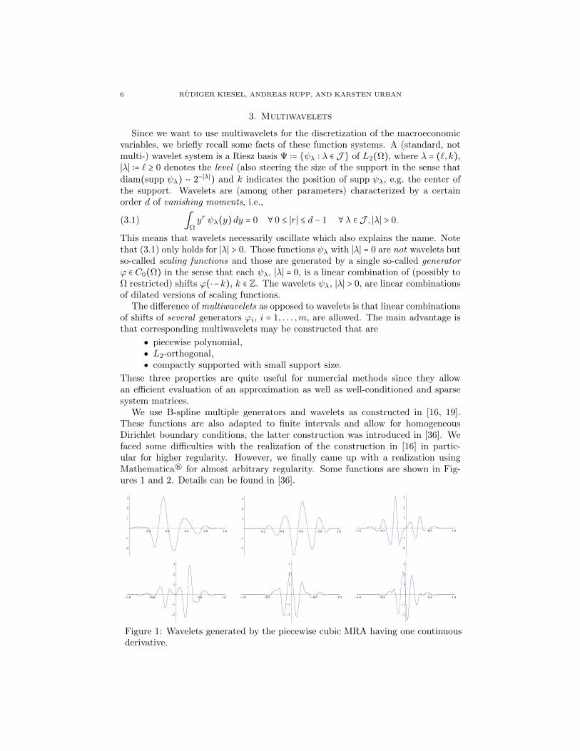
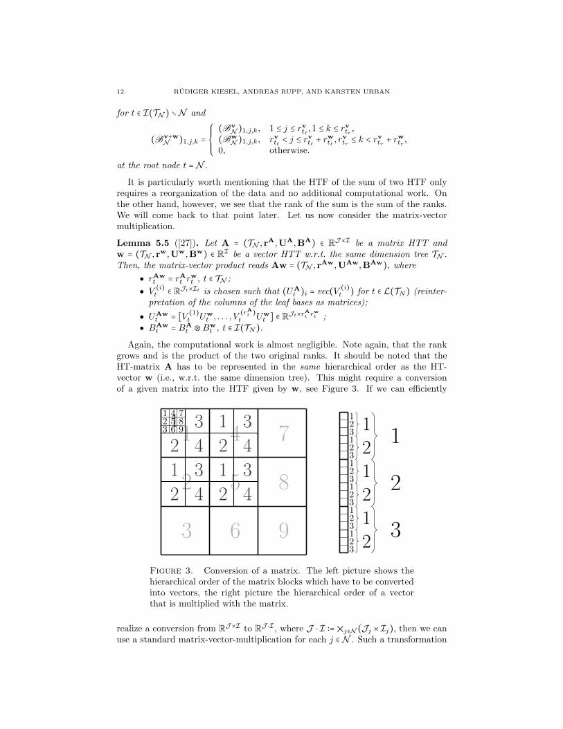
Again, the computational work is almost negligible. Note again, that the rankgrows and is the product of the two original ranks. It should be noted that theHT-matrix A has to be represented in the same hierarchical order as the HT-vector w (i.e., w.r.t. the same dimension tree). This might require a conversionof a given matrix into the HTF given by w, see Figure 3. If we can efficiently
1
2
3
4
5
6
7
8
9
1
2
3
4
1
2
3
4
1
2
3
4
1
2
3
4
123
456
789
123123123123123123212121
3
2
1
Figure 3. Conversion of a matrix. The left picture shows thehierarchical order of the matrix blocks which have to be convertedinto vectors, the right picture the hierarchical order of a vectorthat is multiplied with the matrix.
realize a conversion from RJ×I to RJ ⋅I , where J ⋅ I ∶= ⨉j∈N (Jj × Ij), then we canuse a standard matrix-vector-multiplication for each j ∈ N . Such a transformation

ADAPTIVE MULTIWAVELET METHODS FOR STRUCTURED FINANCIAL PRODUCTS 13
can be done by a reverse lexicographical ordering of the indices, i.e., applying thevec-routine to a matrix-tensor.
Lemma 5.6. Let A = (TN , rA,UA,BA) ∈ RI×I be a square HTT-matrix, then
DA = diag(A) ∈ RI is given as DA = (TN , rA,UDA ,BA), where UDA
t ∈ RIt×rAt is
obtained from UAt ∈ R(It×It)×r
At , t ∈ TN , by (UDA
t )i,k ∶= (UAt )(i,i),k, k = 1, . . . , rAt ,
i ∈ It.
Lemma 5.7. Let AAA = ∑mk=1⊗µ∈N Ak,µ ∈ RK be a Kronecker tensor, then AAA =
(TN , rAAA ,UAAA ,BAAA ), where
UAAAµ ∶= Ak,µ, k = 1, . . . ,m, µ ∈ L(TN ), rAAAµ ∶= k;
for t ∈ I(TN ) ∖ N: BAAAt ∈ Rm×m×m, rAAAt ∶=m and
(BAAAt )i,j,` ∶=
⎧⎪⎪⎨⎪⎪⎩
1, if i = j = `,
0, else;
(BAAAN )i,j,` = δj,`, B
AAAN ∈ R1×k×k, rAAAN ∶= 1.
Remark 5.8. Since the Kronecker sum in Definition A.6 is a special case of aKronecker tensor, Lemma 5.7 also provides an HTF for Kronecker sums.
Truncation of Tensors. We have seen that vector-vector addition and matrix-vectormultiplication can be efficiently done for tensors in HTF. However, by Lemmata 5.4and 5.5 the hierarchical rank grows with each addition or multiplication, so thatonly a certain number of such operations can be done in a numerical (iterative)scheme until the resulting HTTs get too large to be handled efficiently. Thus, atruncation is required.
The basic idea is to apply a singular value decomposition (SVD) on the matri-
cizations w(t) of the tensor w and restrict these to the dominant singular values.This can be realized without setting up w(t) explicitly. Since, by construction, thecolumns of the mode frames Ut contain a basis for the column span of w(t) there
is a matrix Vt ∈ RI(t)×rt such that w(t) = UtV
Tt . Only the left singular vectors of
the SVD of w(t) are thus needed. Thus, the symmetric singular value decomposi-tion of w(t)(w(t))T = UtV
Tt VtU
Tt =∶ UtGtU
Tt yields the same result. The matrices
Gt ∶= VTt Vt ∈ Rrt×rt are called reduced Gramian. They are always of small size and
can be computed recursively within the tree structure. In [20, Lemma 4.6] it isshown, that the reduced Gramians correspond to the accumulated transfer tensorsfor orthogonal HTTs. This statement also holds for general HTTs, see also [27].
The truncation of an HTT can then be computed by the computation of the QRdecomposition Ut = QtRt for t ∈ L(Td) or (STtlRtl ⊗ S
TtrRtr)Bt = QtRt for t ∈ I(Td).
Subsequently, the symmetric eigenvalue decomposition of RtGtRTt = StΣ
2STt is
computed and the truncated matrix is then given by Ut = QtSt, t ∈ L(Td), or
Bt = QtSt, t ∈ I(Td), where St is a restriction of St to the first rt columns. Finally,we recall a well-known estimate for the truncation error.
Lemma 5.9. Let w = (TN , r,U,B) be an HTT and let w = (TN , r, U, B) be the
truncation of w such that rank(w(t)) = rt ≤ rt. Then, for It = 1, . . . , nt, we have
∥w − w∥2 ≤⎛
⎝
nt
∑i=rt+1
σ2i
⎞
⎠
1/2
≤√
2d − 3 infv∈H(r)
∥w − v∥2 ,
14 RUDIGER KIESEL, ANDREAS RUPP, AND KARSTEN URBAN
where H(r) ∶= v = (TN , r,U,B) ∶ rank(v(t)) ≤ rt, t ∈ TN and σi are the sigular
values of w(t) such that σi ≥ σj if i < j, i = 1, . . . , nt.
Together with the vector-vector and matrix-vector addition as well as the trun-cation, the linear solver can be realized, [2]. The main difference is that after eachaddition or multiplication a truncation has to be made in order to keep the hierar-chical rank small, which is not always easy to realize, [27]. For the HTF a Matlabimplementation is available, [27]. We have developed an HT library in C++ in [36]based on BLAS, [8, 14, 15, 28] and LAPACK [1] routines, which are efficiently ac-cessed via the FLENS interface, [29, 30, 31]. The reason for our implementation isthat FLENS is the basis of the LAWA library (Library for Adaptive Wavelet Appli-cations), [40]. The coupling of the proposed adaptive wavelet scheme with the HTstructure could thus be efficiently realized. All subsequent numerical experimentshave been performed with this software.
6. Numerical experiments
We report on numerical experiments, first (in order to describe some fundamentalmechanisms) for a simple CDO and then in a more realistic framework.
6.1. Encoding of defaults. We are given n assets and hence the state dimensionis N = 2n. Let j ∈ N and let j ∈ N ∶= 0,1n be its binary representation, i.e.,a binary vector (j1, . . . ,jn)
T of length n, where ji = 1 means that asset numberi is defaulted. For j, k ∈ N with binary representation j,k ∈ N and j∣k denotingthe bitwise XOR, the number of ones in j∣k corresponds to the number of assetsthat change their state. This easy encoding is the reason why we used the labelingN = 0, . . . ,N − 1.
Once defaulted, always defaulted. For our numerical experiments, we assume forsimplicity that an asset that is defaulted, stays defaulted for all future times, it can-not be reactivated (the theory and our implementation, however, is not restricted tothis case). This means that qj,k(t, y) = 0 if there exists an index 1 ≤ i ≤ n such thatji = 1, ki = 0. Both in the usual and in the binary ordering this last statement meansqj,k(t, y) = 0 if j > k, which in turns means that the Q(t, y) ∶= (qj,k(t, y))j,k∈N is an
upper triangular matrix. Moreover, recall that qj,j(t, y) = −∑k∈N ,k>j qj,k(t, y), so
that Q can be stored as a strict lower triangular matrix, i.e., Q = (qj,k)k>j ∈ RN×N .
Independent defaults. We will always assume that we have independent defaults.If defaults are independent, the transition of asset i from one state to another isindependent of the state for all other assets as long as their states remain unchanged.Before we are going to formalize this, the following example may be helpful for theunderstanding.
Example 6.1. If a portfolio consists of 3 assets, asset 2 defaults when changingfrom state 0 = (000)2 to state 2 = (010)2, from state 1 = (001)2 to state 3 =
(011)2, from state 4 = (100)2 to state 6 = (110)2 and from state 5 = (101)2 tostate 7 = (111)2. These are all transitions where only asset 2 defaults. Whenindependent defaults are assumed, it follows that q0,2 = q1,3 = q4,6 = q5,7. Note that0∣2 = 1∣3 = 4∣6 = 5∣7 = (010)2.
ADAPTIVE MULTIWAVELET METHODS FOR STRUCTURED FINANCIAL PRODUCTS 15
Let j, k ∈ N , then j∣k indicates a state change of asset i if the i-th component ofj∣k is one. Hence, if j1∣k1 = j2∣k2, then the same assets change their state. Sincethe change 1→ 0 is not allowed, we obtain that
j1∣k1 = j2∣k2 ⇒ qj1,k1 = qj2,k2 .
Only one default at a time. If only one asset can default at a time, the transitionintensity qj,k is zero if j∣k has more than one “1”. On the other hand, if j∣k hasonly one “1”, then j∣k must be a power of 2. Since qj,k(t, y) = 0 for j > k, it sufficesto consider the case k > j (qj,j is determined by the condition on the sum over allintensities). For k > j being j∣k a power of 2 means that log2(k − j) ∈ N. In thiscase, we have j∣k = 0∣(k∣j), so that for j, k ∈ N we have
qj,k(t, y) = q0,k∣j(t, y), if k > j and log2(k − j) ∈ N,0, otherwise.
6.2. A model problem. The idea of our first numerical example is to showcase thenumerical manageability, where the focus is on the combination of the multiwaveletcomponents and the high dimensional Markov chain components. To this end, westart with a simplified CDO:
The macroeconomic process Y is one dimensional with parameters α andβ, that are constant in time. This implies that A(t) ≡ A and B(t) ≡ B.
The interest rate r(t) ≡ r is constant in time and does not depend on themacroeconomic process Y .
The state dependent parameters qi,j(t, y) and cj(t, y) are constant in timeand do not depend on the macroeconomic process Y , i.e., hq(y) ≡ 1 and
hc(y) ≡ 1, hence qj,k(t, y) ≡ qj,k and cj(t, y) ≡ cj . This means that Q(t, y) ≡
Q = Q, where Q = (qj,k)k>j;j,k∈N .
There is no recovery and no final payments, i.e., aj,k(t, y) ≡ 0 for all j, k ∈ Nand aj(y) = 0 for j ∈ N .
There is only one tranche covering the entire CDO portfolio.
This means that all involved matrices are time-independent. In particular, wehave Cj,k(t) ≡ γjk ((ψλ, ψµ)0;Ω)λ,µ∈J = γjkIJ . Moreover (Mq)λ,µ = (hqψλ, ψµ)0;Ω =
δλ,µ and D(t) ≡ D = (dj,k)j,k∈N . Next, we have by aj,k(t, y) ≡ 0 that bj(t) ≡ 0,cj(t) ≡ cj , g1
λ = g2λ = (1, ψλ)0;Ω (= 0 for ∣λ∣ > 0) so that (4.3) simplifies to
(6.1) (IN ⊗ IJ )x(t)+ [(IN ⊗ [A+ rIJ ])+ (D⊗ IJ )]x(t) = (−c)⊗ ((1, ψλ)0;Ω)λ∈J .
For later reference, recall that (4.2) in this case implies dk,k = −∑m∈N∖k,m>k qk,m.
In turns, this means that
D = Q + diag(Q1N ), where 1N ∶= (1, . . . ,1)T ∈ RN .
Note that even though D is time-independent, the huge dimension requires storageas an HT-matrix (in particular, it is impossible to store D directly). We use a stan-dard implicit θ-scheme for the time-discretization of this Sylvester-type equation,[42]. The Barlets-Steward algorithm [5], is a well-known method for solving suchSylvester equations. It is based on a Schur decomposition. However, we cannotuse this method here, since, to the best of our knowledge, there is no algorithm forthe QR decomposition of HT-matrices available. Alternatively, an iterative scheme(CG, GMRES or BiCGStab) may be used. We have used BiCGStab as D is (in gen-eral) not symmetric. While generally GMRES yields faster convergence in terms
16 RUDIGER KIESEL, ANDREAS RUPP, AND KARSTEN URBAN
of iteration numbers, it requires more computational steps and therefore, in thecontext of HT-matrices, more truncations are needed, which is computationally ex-pensive. For systems with small condition numbers, BiCGStab requires only a fewiterations, [41]. Using any iterative solver requires matrix-vector multiplications,here of the type (IN ⊗A+D⊗ IJ )x, where x = x1⊗x2 is also a Kronecker productof the appropriate dimension. Then, we obtain
(IN ⊗A +D⊗ IJ )(x1 ⊗ x2) = x1 ⊗Ax2 +Dx1 ⊗ x2,
which can be represented as a Kronecker product of an HT-matrix and a matrix.For details of the implementation, we refer to [36].
6.2.1. Construction of the intensity matrix D. We describe the representation ofD into HTF in case of independent defaults and only one default at a time. Recallthat D = Q+diag(Q1N ) and Q = (qj,k)k>j ∈ RN×N . Hence, we start by deriving a
Kronecker sum representation for Q.
Theorem 6.2. In case of independent defaults and one default at a time, the matrixQ ∈ RN×N can be written as a Kronecker sum (see Definition A.6 below)
(6.2) Q =n
⊕k=1
(0 q0,2n−k
0 0) =
n
∑k=1
k−1
⊗`=1
I2×2 ⊗ (0 q0,2n−k
0 0)⊗
n
⊗`=k+1
I2×2 ,
where I2×2 ∈ R2×2 denotes the identity matrix of corresponding size.
Proof. The k-th summand of the Kronecker sum on the right-hand side of (6.2)reads
Qk ∶=k−1
⊗`=1
I2×2 ⊗ (0 q0,2n−k
0 0)⊗
n
⊗`=k+1
I2×2.
It is readily seen that Qk is a matrix having the entries q0,n−k at the positions
(2n−k+1(ν − 1) + µ, 2n−k+1
(ν − 1) + µ + 2n−k),
for ν = 1, . . . ,2k−1 and µ = 1, . . . ,2n−k, i.e., 2k−1 ⋅2n−k = 2n−1 entries. Note that 2n−1
is the number of all combinations with a state change of asset k. Since 2n−k+1(ν −1) + µ ≠ 2n−k for all possible ν and µ, we obtain that j∣k has exactly one “1” at
position i = n − k. This, in turns, means that qj,k = q0,n−k. This shows that Qk
contains all transition intensities corresponding to asset k at the right positions.It remains to show that the sum over all Qk does not cause overlapping indices.
Since ⊕k−1`=1 I2×2 ∈ R2k−1×2k−1 , each Qk is a block matrix with blocks at different
positions. Thus ⊕nk=1 Qk collects the transition intensities for all assets k.
Having the Kronecker sum (6.2) at hand, the next step is to derive the HTF of D.
As we have seen in Lemma 5.7 and Remark 5.8, the HTF of Q can easily be derivedfrom the Kronecker sum representation. Next, note that RN ∋ 1N = ⊗
nk=1(1,1)
T ,
so that the HTF of Q1N can be obtained via Lemma 5.6 and the HTF of D byLemma 5.4. Finally, it is easily seen that c =⊕
nk=1(ck,0)
T so that the HTF of theright-hand side is easily be derived.

ADAPTIVE MULTIWAVELET METHODS FOR STRUCTURED FINANCIAL PRODUCTS 17
6.2.2. Results. We have used fictional data as marked data is generally not pub-licly available for CDOs. The fictional CDO portfolio consists of n = 128 assets,which is a reasonable size. The macroeconomic process is assumed to be one di-mensional. This leads to a system of N = 2128 coupled partial differential equations.The maturity is assumed to be T = 1 and the time interval is discretized into 20time steps. For the Galerkin approximation, piecewise cubic L2-orthonormal Multi-wavelets with Dirichlet boundary conditions. We have fixed the lowest and highestlevel to j0 = 2 and J = 4. This turned out to be sufficient in this example due tothe smoothness of the right-hand side. For the θ-scheme, the parameter θ = 0.5 hasbeen chosen (Crank-Nicholson). To solve the linear system, BiCGStab has beenused. The stopping criterion of the linear solver has been set as a relative error ofthe L2-norm of the residual to 10−13 and HTTs are truncated to a rank of 5.
00.2
0.40.6
0.81 0
0.20.4
0.60.8
0100200300400500600700800
u
t
y
u
00.2
0.40.6
0.81 0
0.20.4
0.60.8
−1.0 10−14
0.0 10−14
1.0 10−14
2.0 10−14
3.0 10−14
4.0 10−14
5.0 10−14
6.0 10−14
u
t
y
u
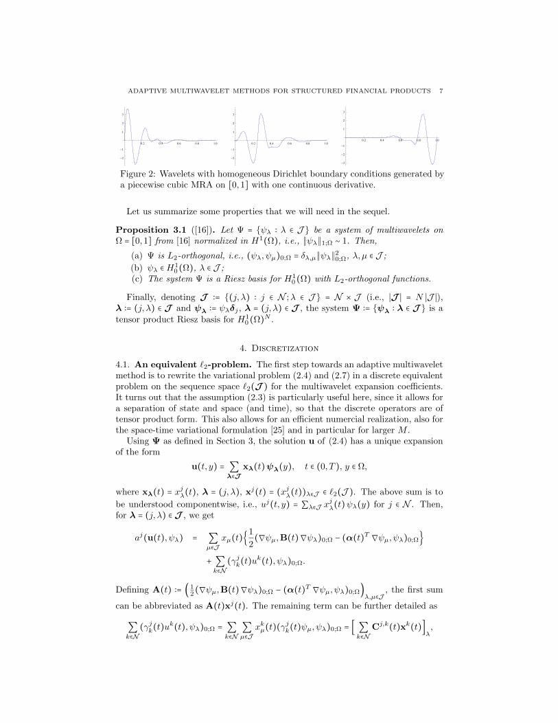
Figure 4. CDO portfolio value in a portfolio of 128 assets. Firststate (no defaults, left) and state (all firms have defaulted, right).Note the scaling of the vertical axis in the right figure.
In Figure 4, left, the portfolio value depending on the time t and the macroeco-nomic state y of the CDO in the first stage, where no firm has defaulted, is shown.Whenever a firm defaults, the Markov chain changes its state and the portfoliovalue jumps to a lower value due to the immediate loss of all future continuous pay-ments. To illustrate the jumps of the portfolio value, when a default has occurred,the values of all states of a portfolio of 2 assets have been combined in Figure 5,left. The last stage is used for error analysis, since here the portfolio value has tobe zero as all firms have defaulted. Figure 4 shows on the right the portfolio valuein the last state of this simulation. This can be interpreted as the relative errorarising from the Galerkin approximation with the L2-orthonormal multiwaveletsand the truncation of the HTTs after each addition or multiplication. It can beobserved, that the relative error of this computation is smaller than 10−13, whichcorresponds to the stopping criterion of the linear solver. In each time step, theBiCGStab algorithm took on average 54 iterations.
The computations were performed on a Dell XPS with Intel T9300 Dual CoreCPU and 3GB storage and took about 1 hour, the runtime for different portfoliosizes is summarized in Figure 5, right. We observe a linear scaling with respect ton, i.e., only a logarithmic scaling compared to the number of equations N = 2n.
6.3. A realistic scenario. The example presented in the previous section corre-sponds to a simplified and idealized situation. As we will show now, the extensionto a realistic scenario (given sufficient data), is not too difficult. In fact:
Observe, that time-dependent parameters do not affect the runtime of thepricing as the condition number of the matrix is not affected, assuming theparameters are sufficiently smooth in the time t.
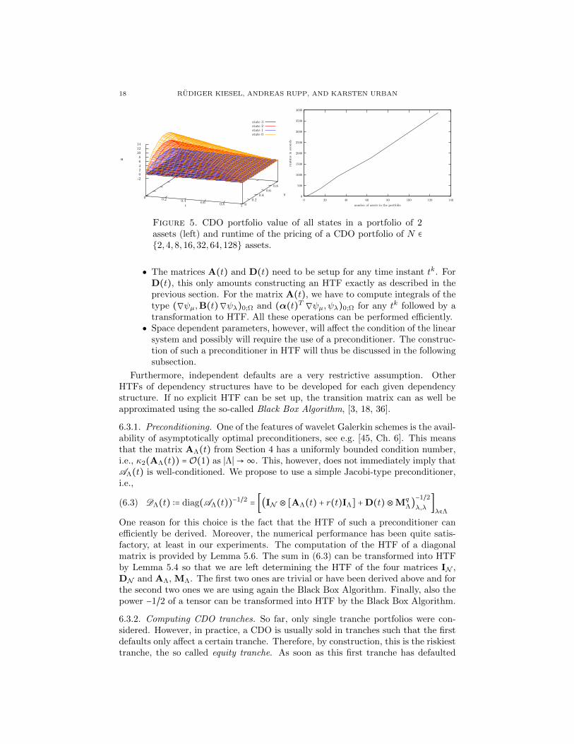
18 RUDIGER KIESEL, ANDREAS RUPP, AND KARSTEN URBAN
0 0.2 0.4 0.6 0.8 1 00.2
0.40.6
0.8
-202468
101214
u
state 3state 2state 1state 0
t
y
u
0
500
1000
1500
2000
2500
3000
3500
4000
0 20 40 60 80 100 120 140
runti
me
inse
con
ds
number of assets in the portfolio
Figure 5. CDO portfolio value of all states in a portfolio of 2assets (left) and runtime of the pricing of a CDO portfolio of N ∈
2,4,8,16,32,64,128 assets.
The matrices A(t) and D(t) need to be setup for any time instant tk. ForD(t), this only amounts constructing an HTF exactly as described in theprevious section. For the matrix A(t), we have to compute integrals of thetype (∇ψµ,B(t)∇ψλ)0;Ω and (α(t)T ∇ψµ, ψλ)0;Ω for any tk followed by atransformation to HTF. All these operations can be performed efficiently.
Space dependent parameters, however, will affect the condition of the linearsystem and possibly will require the use of a preconditioner. The construc-tion of such a preconditioner in HTF will thus be discussed in the followingsubsection.
Furthermore, independent defaults are a very restrictive assumption. OtherHTFs of dependency structures have to be developed for each given dependencystructure. If no explicit HTF can be set up, the transition matrix can as well beapproximated using the so-called Black Box Algorithm, [3, 18, 36].
6.3.1. Preconditioning. One of the features of wavelet Galerkin schemes is the avail-ability of asymptotically optimal preconditioners, see e.g. [45, Ch. 6]. This meansthat the matrix AΛ(t) from Section 4 has a uniformly bounded condition number,i.e., κ2(AΛ(t)) = O(1) as ∣Λ∣→∞. This, however, does not immediately imply thatAΛ(t) is well-conditioned. We propose to use a simple Jacobi-type preconditioner,i.e.,
(6.3) DΛ(t) ∶= diag(AΛ(t))−1/2= [(IN ⊗ [AΛ(t) + r(t)IΛ] +D(t)⊗Mq
Λ)−1/2λ,λ
]λ∈Λ
One reason for this choice is the fact that the HTF of such a preconditioner canefficiently be derived. Moreover, the numerical performance has been quite satis-factory, at least in our experiments. The computation of the HTF of a diagonalmatrix is provided by Lemma 5.6. The sum in (6.3) can be transformed into HTFby Lemma 5.4 so that we are left determining the HTF of the four matrices IN ,DN and AΛ, MΛ. The first two ones are trivial or have been derived above and forthe second two ones we are using again the Black Box Algorithm. Finally, also thepower −1/2 of a tensor can be transformed into HTF by the Black Box Algorithm.
6.3.2. Computing CDO tranches. So far, only single tranche portfolios were con-sidered. However, in practice, a CDO is usually sold in tranches such that the firstdefaults only affect a certain tranche. Therefore, by construction, this is the riskiesttranche, the so called equity tranche. As soon as this first tranche has defaulted
ADAPTIVE MULTIWAVELET METHODS FOR STRUCTURED FINANCIAL PRODUCTS 19
completely, subsequent defaults begin to affect a second trance. Therefore, this sec-ond tranche, called mezzanine tranche, is less risky than the first one. And finally, ifthis second tranche also has defaulted, the last tranche, the so called senior trancheis affected. Sometimes, these three tranches can be further split into sub-tranches.To compute the price of a CDO tranche, the cash flows of (1.1a) have to be adaptedto the cash flows which affect the tranche under consideration. The constructionof these adapted parameters is described in the following.
Given a portfolio of n assets with nominal values π1, . . . , πn, the S tranches aredefined by their upper boundary bs, s = 1, . . . , S, given in percentages b0 = 0 <
b1 < ⋯ < bS−1 < bS = 1 of the total portfolio nominal Π ∶= ∑ni=1 πi. Let Lj be the
accumulated loss in state j ∈ N , i.e., Lj = ∑i∈D(j) πi, where
D(j) ∶= i ∈ 1, . . . , n ∣ ∃xk ∈ 0,1, k = 1, . . . , n, xi = 1 ∶ j =n
∑k=1
xk2k−1
denotes the set of all defaulted firms in state j. Then, the cash flows are distributedas follows:
The amount of the state dependent continuous payments cj which is as-signed to the s-th tranche, s = 1, . . . , S, in state j ∈ N can be computed asthe percentage of the nominal of the tranche divided by the accumulatednominals of the assets not in default:
(6.4) cjs(t) =
⎧⎪⎪⎪⎪⎪⎨⎪⎪⎪⎪⎪⎩
cj(t)Π(bs−bs−1)Π−Lj if Lj < Πbs−1
cj(t)Π(1−bs)−LjΠ−Lj if Πbs−1 ≤ L
j < Πbs,
0 otherwise.
The final payments ujT are distributed to the tranches in the same way as
the continuous payments c, i.e., (6.4) holds with cjs(t) replaced by ujT,s, thefinal payment of tranche number s.
The recovery payments are paid out as a single payment to the tranche inwhich the default occurred.
If several tranches are affected, the recovery is paid out proportional totheir nominals. This means
aj,ks (t) =
⎧⎪⎪⎪⎪⎪⎪⎪⎪⎨⎪⎪⎪⎪⎪⎪⎪⎪⎩
aj,k(t) if Πbs−1 < Lj < Lk ≤ Πbs,
aj,k(t)Lk−Πbs−1Lk−Lj if Lj ≤ Πbs−1 < L
k ≤ Πbs,
aj,k(t)Πbs−Πbs−1Lk−Lj if Lj ≤ Πbs−1 < Πbs < L
k,
aj,k(t)Πbs−LjLk−Lj if Πbs−1 < L
j ≤ Πbs < Lk.
In this setting only recoveries are considered, when a default occurs. How-ever, the model also allows for firms to be in default only temporarily. Thismeans, there can also be payments if Lk < Lj . These cases are omitted inthe following as they can be handled exactly as the cases where Lj < Lk.
The difficulty of computing the payoffs of the s-th tranche is that certain specificstates within the huge amount of states of the Markov chain have to be found.Therefore, we define vectors 1<s , 1
=s and 1>s , by
(1<s)j ∶= χLj<Πbs−1, (1=s)j ∶= χΠbs−1≤Lj<Πbs, (1>s)j ∶= χLj≥Πbs, j ∈ N .
In order to explain the realization of some required operations, we introduce thefollowing short-hand nottaion for HTTs. Let w ∈ RK be a tensor with HTF w =
20 RUDIGER KIESEL, ANDREAS RUPP, AND KARSTEN URBAN
(TN , r,U,B), then we abbreviate by H(w) its HTF without specifying the quanti-ties involved in the HTF. For A ∈ RK×K and b ∈ RK, we indicate by H(A)H(u) =
H(b) that u ∈ RK is determined as the solution of the linear system Au = bbut only with numerical routines using the HTF-variants. Finally, we abbreviateD(w) ∶=H(diag(w)) ∈ RK for w ∈ RK, where (diag(w))i,j ∶= δi,j wi, i ∈ K.
Now, denote L ∶= (Lj)j∈N . Then, we need to compute the reciprocal value of each
component of the vector R ∶= Π − L ∈ RN in HTF denoted by R(−1). This can beachieved by solving the linear system D(H(R))x =H(1) for x. Then H(R(−1)) ∶= xand
H(cs(t)) = D(H(c(t))D(H(R−1))H(1<µ)Π(bs − bs−1)
+D(H(c(t))D(H(R−1))D(H(1=µ))(Π(1 − bs)H(1) −H(L)).
We obtain a similar formula for the final payments (ujT,s)j∈N . The HTF of the
matrix As(t) ∶= (aj,ks (t))j,k∈N can be set up similarly. Therefore, the matrix
S ∶= (Lk − Lj)j,k∈N is required. The HTF of this matrix can be obtained byH(S) = H(1 ⋅ 1T )D(H(L)) − D(H(L))H(1 ⋅ 1T ). As before, the HTF of the
matrix S(−1) containing the reciprocals of the entries of S can be found by solv-ing D(S)x = H(1) for x and setting H(S(−1)) ∶= x. Defining finally A (v,w) ∶=
D(H(v))H((ai,j(t))i,j∈N )D(H(w)), we obtain
H(As(t)) = A (1=s ,1=s)
+D(A (1<s ,1=s))D(H(S(−1)
))(H(1 ⋅ 1T )(D(H(L)) −D(H(1))Πbs−1))
+D(A (1<s ,1>s))D(H(S(−1)
))(H(1 ⋅ 1T )(D(H(1))Π(bs − bs−1))
+D(A (1=s ,1>s))D(H(S(−1)
))(H(1 ⋅ 1T )(D(H(1))Πbs) −D(H(L))).
With these adapted payments, the value of a portfolio tranche can now be deter-mined. A key point of this approach is the construction of the HTF of the vectors1<s , 1
=s and 1>s . This can be computed by
H(1<s) ∶= maxΠbs−1H(1) −H(L),0 (Πbs−1H(1) −H(L))−1,
H(1>s) ∶= maxH(L) −ΠbsH(1),0 (H(L) −ΠbsH(1))−1,
H(1=s) ∶=H(1) −H(1<s) −H(1>s).
The component-wise maximum maxH(⋅),0 of any HT-vector can be determinedby the relation maxH(⋅),0 = 1
2(H(⋅) + ∣H(⋅)∣). The absolute value ∣H(w)∣ can be
computed by the component-wise Newton iteration
H(w(n+1)) =H(w(n)) −D((H(w(n)))−1
)D(H(w))H(w).
Note, that each iteration step requires the component-wise inversion of an HT-vector, i.e., the solution of a linear system. Let ν be such that w(ν) is of the desired
accuracy, then ∣H(w)∣ ≈ H(w(ν)). Essentially, this corresponds to ∣x∣ =√x2, the
well-known Babylonian method, which converges quadratically for non-zero values.Moreover, for vectors w(0) with positive entries, it always converges to the positivesolution.
Appendix A. The Kronecker Product
The Kronecker product is a well-known technique when dealing with high dimen-sional problems, as it often allows the decomposition of a high dimensional problem
ADAPTIVE MULTIWAVELET METHODS FOR STRUCTURED FINANCIAL PRODUCTS 21
into a product of problems of low dimension. The following facts can be found in[39, 47].
Definition A.1. The Kronecker product A ⊗ B ∈ RmAmB×nAnB of two matri-ces A ∈ RmA×nA and B ∈ RmB×nB is defined by (A ⊗ B)(µ1−1)mB+µ2,(ν1−1)nB+ν2 ∶=Aµ1,ν1Bµ2,ν2 .
We note that the above definition and all subsequent properties can also beextended to (infinite) countable index sets J .
Lemma A.2. Let A ∈ RmA×nA , B ∈ RmB×nB , C ∈ RmC×nC , D ∈ RmD×nD and ν ∈ R.Then,
(1) (A⊗B)T = AT ⊗BT ,(2) (A⊗B)−1 = A−1 ⊗B−1,(3) (A⊗B)(C ⊗D) = AC ⊗BD, if nA =mC and nB =mD,(4) A⊗ (B ⊗C) = (A⊗B)⊗C,(5) A⊗ (B +C) = A⊗B +A⊗B and (B +C)⊗A = B ⊗A +C ⊗A,(6) ν(A⊗B) = (νA)⊗B = A⊗ (νB),(7) tr(A⊗B) = tr(A)tr(B),(8) if mA = nA and mB = nB, then det(A⊗B) = (det(A))
nB (det(B))nA ,
(9) rank(A⊗B) = rank(A)rank(B).
Definition A.3. Let A ∈ RmA×nA , then its vectorization is defined as vec(A) =
(AT⋅,1, . . . ,AT⋅,nA)
T , where A⋅,i, i ∈ 1, . . . , nA, is the i-th column of the matrix A.
Lemma A.4 ([47, (2)]). Let A ∈ RmA×nA ,B ∈ RmB×nB ,C ∈ RmB×mA ,X ∈ RnB×nA ,then (A⊗B)vec(X) = vec(C)⇔ BXAT = C.
Definition A.5. Let Ak,µ ∈ RKµ , µ ∈ N , k = 1, . . . ,m, m ∈ N. Then, we define theKronecker tensor as
AAA ∶=m
∑k=1
⊗µ∈N
Ak,µ ∈ RK.
Definition A.6. Let A1, . . . ,Am be matrices Ak ∈ Rnk×nk . Then, the Kroneckersum of A1, . . . ,Am is defined as
(A.1)m
⊕k=1
Ak ∶=m
∑k=1
k−1
⊗`=1
In`×n` ⊗Ak ⊗m
⊗`=k+1
In`×n` ∈ R(n1⋯nm)×(n1⋯nm).
Obviously, the Kronecker sum is a special case of the Kronecker tensor, whereAk,µ = δk,`Ak + (1 − δk,`)In`×n`
References
[1] E. Anderson, Z. Bai, C. Bischof, S. Blackford, J. Demmel, J. Dongarra, J. Du Croz, A. Green-baum, S. Hammarling, A. McKenney, and D. Sorensen. LAPACK Users’ Guide. Society forIndustrial and Applied Mathematics, Philadelphia, PA, third edition, 1999.
[2] J. Ballani and L. Grasedyck. A projection method to solve linear systems in tensor format.
Numerical Linear Algebra with Applications, 20(1):27–43, 2013.[3] J. Ballani, L. Grasedyck, and M. Kluge. Black box approximation of tensors in hierarchical
tucker format. Linear Algebra and its Applications, 438(2):639–657, 2013.[4] M. Barrault, Y. Maday, N.C. Nguyen, and A.T. Patera. An ‘empirical interpolation’ method:
application to efficient reduced-basis discretization of partial differential equations. C. R.Math. Acad. Sci. Paris, 339(9):667–672, 2004.
[5] R. H. Bartels and G. W. Stewart. Solution of the matrix equation ax + xb = c [f4]. Commun.
ACM, 15(9):820–826, September 1972.
22 RUDIGER KIESEL, ANDREAS RUPP, AND KARSTEN URBAN
[6] P. Beaudry and A. Lahiri. Risk allocation, debt fueled expansion and financial crisis. Working
Paper 15110, National Bureau of Economic Research, June 2009.
[7] T. R. Bielecki and M. Rutowski. Credit Risk: Modeling, Valuation and Hedging. Springer,2002.
[8] L. S. Blackford, J. Demmel, J. Dongarra, I. Duff, S. Hammarling, G. Henry, M. Heroux,
L. Kaufman, A. Lumsdaine, A. Petitet, R. Pozo, K. Remington, and R. C. Whaley. Anupdated set of basic linear algebra subprograms (blas). ACM Trans. Math. Softw., 28(2):135–
151, June 2002. http://www.netlib.org/blas/.
[9] C. Bluhm and L. Overbeck. Structured Credit Portfolio Analysis, Baskets and CDOs. Chap-man and Hall, 2007.
[10] A. Cohen, W. Dahmen, and R. DeVore. Adaptive wavelet methods for elliptic operator equa-
tions: convergence rates. Math. Comp., 70(233):27–75, 2001.[11] A. Cohen, W. Dahmen, and R. DeVore. Adaptive wavelet methods. II. Beyond the elliptic
case. Found. Comput. Math., 2(3):203–245, 2002.[12] A. Cohen, W. Dahmen, and R. Devore. Adaptive wavelet schemes for nonlinear variational
problems. SIAM J. Numer. Anal., 41(5):1785–1823, 2003.
[13] T. J. Dijkema, C. Schwab, and R. Stevenson. An adaptive wavelet method for solving high-dimensional elliptic pdes. Constructive Approximation, 30:423–455, 2009.
[14] J. J. Dongarra, J. Du Croz, S. Hammarling, and I. S. Duff. A set of level 3 basic linear algebra
subprograms. ACM Trans. Math. Softw., 16(1):1–17, 1990. http://www.netlib.org/blas/.[15] J. J. Dongarra, J. Du Croz, S. Hammarling, and R. J. Hanson. An extended set
of fortran basic linear algebra subprograms. ACM Trans. Math. Softw., 14:1–17, 1986.
http://www.netlib.org/blas/.[16] G. Donovan, J. Geronimo, and D. Hardin. Orthogonal polynomials and the construction of
piecewise polynomial smooth wavelets. SIAM J. Math. Anal., 30(5):1029–1056, 1999.
[17] G. P. Dwyer. Financial innovation and the financial crisis of 2007-2008. Papeles de EconomiaEspana, 130, 2012.
[18] M. Epsig, L. Grasedyck, and W. Hackbusch. Black box low tensor-rank approximation usingfiber-crosses. Constructive Approximation, 30(3):557–597, 2009.
[19] J. S. Geronimo, D. P. Hardin, and P. R. Massopust. Fractal functions and wavelet expansions
based on several scaling functions. J. Approx. Theory, 78(3):373–401, 1994.[20] L. Grasedyck. Hierarchical singular value decomposition of tensors. SIAM Journal on Matrix
Analysis and Applications, 31(4):2029–2054, 2010.
[21] W. Hackbusch and S. Kuhn. A new scheme for the tensor representation. Journal of FourierAnalysis and Applications, 15(5):706–722, 2009.
[22] N. Hilber, S. Kehtari, C. Schwab, and C. Winter. Wavelet finite element method for option
pricing in highdimensional diffusion market models. Research Report 01, ETH Zurich, 2010.[23] R. A. Jarrow. The role of abs, cds and cdos in the credit crisis and the economy. Working
Paper, 2012.
[24] S. Kestler. On the Adaptive Tensor Product Wavelet Galerkin Method with Applications inFinance. PhD thesis, Ulm University, 2013.
[25] S. Kestler, K. Steih, and K. Urban. An efficient space-time adaptive wavelet galerkin methodfor time-periodic parabolic partial differential equations. Research Report 06, Ulm University,
Fac. of Mathematics and Economics, August 2013.
[26] H. Kraft and M. Steffensen. Bankruptcy, counterparty risk, and contagion. Review of Finance,11:209–252, 2006.
[27] D. Kressner and C. Tobler. htucker - a matlab toolbox for tensors in hierarchical tuckerformat. Preprint, 2012.
[28] C. L. Lawson, R. J. Hanson, D. R. Kincaid, and F. T. Krogh. Basic linear algebra sub-
programs for fortran usage. ACM Trans. Math. Softw., 5(3):308–323, September 1979.
http://www.netlib.org/blas/.[29] M. Lehn. FLENS - a flexible library for efficient numerical solutions. PhD thesis, Ulm Uni-
versity, 2008.[30] M. Lehn. Flexible Library for Efficient Numerical Solutions (FLENS), 2013.
http://apfel.mathematik.uni-ulm.de/~lehn/FLENS/index.html.
[31] M. Lehn, A. Stippler, and K. Urban. Flens - a flexible library for efficient numerical solutions.In Proceedings of Equadiff 11, pages 467–473. Comenius University Press, 2007.
ADAPTIVE MULTIWAVELET METHODS FOR STRUCTURED FINANCIAL PRODUCTS 23
[32] R.H. Nochetto, K.G. Siebert, and A. Veeser. Theory of adaptive finite element methods:
an introduction. In R. DeVore and A. Kunoth, editors, Multiscale, nonlinear and adaptive
approximation, pages 409–542. Springer, Berlin, 2009.[33] A. Nouy. A priori model reduction through proper generalized decomposition for solving
time-dependent partial differential equations. Comput. Methods Appl. Mech. Engrg., 199(23-
24):1603–1626, 2010.[34] D. Pfluger. Spatially Adaptive Sparse Grids for High-Dimensional Problems. PhD thesis,
Technische Universitat Munchen, 2010.
[35] C. Reisinger and G. Wittum. Efficient hierarchical approximation of high-dimensional optionpricing problems. SIAM J. Sci. Comput., 29(1):440–458, January 2007.
[36] A. J. Rupp. High Dimensional Wavelet Methods for Structured Financial Products. PhD
thesis, University of Ulm, 2013.[37] C. Schwab and R. Stevenson. Space-time adaptive wavelet methods for parabolic evolution
problems. Math. Comp., 78(267):1293–1318, 2009.[38] C. Schwab and R. P. Stevenson. Fast evaluation of nonlinear functionals of tensor product
wavelet expansions. Numer. Math., 119(4):765–786, 2011.
[39] W. H. Steeb and T. K. Shi. Matrix Calculus and Kronecker Product With Applications andC++ Programs. World Scientific Publishing Company, Incorporated, 1997.
[40] A. Stippler. Lawa - library for adaptive wavelet applications, 2013.
”http://lawa.sourceforge.net/index.html”.[41] F. D. Swesty, D. C. Smolarski, and P. E. Syalor. A comparison of algorithms for the efficient
solution of the linear systems arising from multigroup flux-limited diffusion problems. The
Astrophysical Journal, 153:369–387, 2004.[42] J. J. Sylvester. Sur l’equations en matrices px = xq. Comptes Redus Acad. Sci. Paris, 99:67–
71, 1884.
[43] J. M. Tavakoli. Collateralized Debt Obligations and Structured Finance. John Wiley and Sons,Inc., 2003.
[44] L. R. Tucker. Some mathematical notes on three-mode factor analysis. Psychometrika,31(3):279–311, 1966.
[45] K. Urban. Wavelet Methods for Elliptic Partial Differential Equations. Oxford University
Press, 2009.[46] K. Urban and A. T. Patera. A new error bound for reduced basis approximation of parabolic
partial differential equations. C.R. Math., 350(3–4):203 – 207, 2012.
[47] C. F. van Loan. The ubiquitous kronecker product. Journal of Computational and AppliedMathematics, 123(1-2):85–100, 2000. Numerical Analysis 2000. Vol. III: Linear Algebra.
Rudiger Kiesel Lehrstuhl fur Energiehandel und Finanzdienstleistungen, University
of Duisburg-Essen, Universitatsstr. 12, D-45117 Essen, GermanyE-mail address: [email protected]
Andreas Rupp, Institute for Numerical Mathematics, University of Ulm, Helmholtz-
strasse 20, D-89069 Ulm, GermanyE-mail address: [email protected]
Karsten Urban, Institute for Numerical Mathematics, University of Ulm, Helm-holtzstrasse 20, D-89069 Ulm, Germany
E-mail address: [email protected]


![Enabling scalable parallel implementations of structured ...parashar/Papers/... · Grid Adaptive Computational Engine (GrACE) [20] is an adaptive computational and data-management](https://img.pdfslide.us/doc/110x75/5f701adcbcfeb05565181e22/enabling-scalable-parallel-implementations-of-structured-parasharpapers.jpg)