A Solution Adaptive Structured/Unstructured Overset Grid ... · PDF fileA Solution Adaptive Structured/Unstructured Overset Grid ... A SOLUTION ADAPTIVE STRUCTURED/UNSTRUCTURED OVERSET

NASA-CR-2O1053

Research Institute for Advanced Computer ScienceNASA Ames Research Center

A Solution AdaptiveStructured/Unstructured Overset Grid

Flow Solver with Applications toHelicopter Rotor Flows

Earl P. N. DuqueRupak Biswas

Roger C. Strawn

RIACS Technical Report 95.09 April 1995

Paper No. AIAA-95-1766, presented at the AIAA 13th Applied Aerodynamics Conference,

San Diego, California, June 19-21, 1995

https://ntrs.nasa.gov/search.jsp?R=19960023578 2018-05-08T15:17:53+00:00Z

A Solution AdaptiveStructured/Unstructured Overset Grid

Flow Solver with Applications toHelicopter Rotor Flows

Earl P. N. DuqueRupak Biswas

Roger C. Strawn

The Research Institute of Advanced Computer Science is operated by Universities Space Research

Association, The American City Building, Suite 212, Columbia, MD 21044, (410) 730-2656

Work reported herein was supported by NASA via Contract NAS 2-13721 between NASA and the Universities

Space Research Association (USRA). Work was performed at the Research Institute for Advanced Computer

Science (RIACS), NASA Ames Research Center, Moffett Field, CA 94035-1000.

AIAA-95-1766

A SOLUTION ADAPTIVE STRUCTURED/UNSTRUCTURED OVERSET GRID FLOW

SOLVER WITH APPLICATIONS TO HELICOPTER ROTOR FLOWS

Earl P.N. Duque

US Army Aeroflightdynamics Directorate, ATCOM, NASA Ames Research Center, Moffett Field, CA

Rupak Biswas

R1ACS, NASA Ames Research Center, Moffett Field, CA

Roger C. StrawnUS Army Aeroflightdynamics Directorate, ATCOM, NASA Ames Research Center, Moffett Field, CA

Abstract

This paper summarizes a method that solves both thethree dimensional thin-layer Navier-Stokes equationsand the Euler equations using overset structured andsolution adaptive unstructured grids with applications tohelicopter rotor fiowfields. The overset structured gridsuse an implicit finite-difference method to solve thethin-layer Navier-Stokes/Euler equations while theunstructured grid uses an explicit finite-volume methodto solve the Euler equations. Solutions on a helicopterrotor in hover show the ability to accurately convect therotor wake. However, isotropic subdivision of thetetrahedral mesh rapidly increases the overall problemsize.

Introduction

A helicopter rotor blade generates a vortical wake

that has a large effect on its performance, vibrations and

noise. In order to accurately predict the performance of

the rotor system, a numerical method must capture this

important feature. In the past, numerical methods have

relied upon empirically based models to approximate

the wake effect (references [1] - [71). More recently,researchers have used various CFD methods such as

vorticity confinement coupled with full potential [8] andEuler or Navier-Stokes with periodic boundary condi-

tions ([9] and [10]) in attempts to compute the wake

structure from first principles.

All the methods mentioned above use single-block,

body-conforming structured grids to discretize the entire

flow field. Topological restrictions in single-block grids

tend to degrade their efficient use in simulations of heli-

copter rotors. For example, single-block grids tend to

have excessive and poorly placed grid points that

increase required computer time, in-core memory and

This paper is declared a work of the U.S. Governmentand is not subject to copyright protection in the UnitedStates.

Presented at the 13th AIAA Applied Aerodynamics Con-ference, San Diego, CA, June 19-21, 1995.

computer costs. Also, it is extremely difficult, if not

impossible, to employ single-block grid schemes for

rotor-body interactions where the relative motion

between aircraft components is important.

In response to these disadvantages, two methodolo-

gies have emerged. One method, by Barth [11] and

modified for rotary wing flows by Strawn and Barth

[12], uses unstructured adaptive grids and an explicittime-integration finite-volume scheme. This method has

the ability to readily refine the grid around flow struc-

tures as demonstrated by Strawn et. al. [13]. However,

insufficient computer resources, inherent grid genera-

tion difficulties and solution accuracy within shear lay-

ers all tend to complicate large three-dimensional

viscous flowfield computations.

Duque and Srinivasan [141 and Meakin [151 use

overset structured grids for rotor computations. Theoverset grids allow for well formed grids at the rotor

surface and separate grids to carry the wakes. These

structured grid methods use implicit solution methods

that allow for larger time steps compared to explicit

methods. However, current structured grid methods are

not well suited for three dimensional grid adaption for

vortex wakes and cannot adequately adapt to an

unsteady flowfield.

In contrast, dynamic unsteady remeshing and gridadaptation on unstructured grids has been presented by

Lohner [16]. The ability to freely remove and add points

within regions of interest is a major advantage of

unstructured grids. In the wake of a helicopter blade, the

solution method needs to resolve the convecting tip vor-

tex and the vortex sheet. Unstructured grid methods

work well within these flow regions. In addition, grids

in this region do not require to be as fine as in viscousboundary layer regions near body surfaces. Therefore,

the CFL limit of an explicit method does not constrain

the time step.

In this paper, the advantages of structured and

unstructured schemes are combined into a hybrid

method that solves both the three dimensional thin-layerNavier-Stokes equations and Euler equations using

overset structured and unstructured grids. The overset

structuredgridsusethe methodologydeveloped by

Srinivasan, et. al. [10]. The structured grids are overset

onto an unstructured grid. The unstructured grid solu-

tion uses the method developed by Barth [11]. The

unstructured grid adapts to the solution using the suc-

cessive edge refinement and coarsening method of Bis-was and Strawn [17].

The main objective of this paper is to determine grid

adaption requirements for general helicopter wakes. Ahelicopter wake is unsteady and can interact with the

oncoming blades. It consists of a tip vortex, root vortex

and a vortical wake sheet. The paper presents a helicop-ter rotor in hover as a model problem and uses a number

of different indicators to determine where to adapt the

unstructured grid. An attempt is made to find an optimal

indicator to identify helicopter wake regions. Results

show that the current mesh adaption scheme can suc-

cessfully refine the grid in rotor wake regions. However,isotropic subdivision of the tetrahedral elements tends to

significantly increase the computer costs.

Mr,tkgaglg.

The structured grid flow solver is that by Srinivasan,

et. al. [10]. This method solves the thin-layer Navier-Stokes equations shown in Equation 1.

(EQ 1)

Reference [10] describes the finite-difference

implicit numerical scheme used for the solution of

Equation 1. Briefly, the numerical algorithm spatially

differences the flux terms using a Roe upwind-biased

scheme for all three coordinate directions with higher-

order MUSCL-type limiting to model shocks accurately.The method advances the solution in time using the LU-

SGS (lower-upper symmetric Gauss-Seidei) implicitscheme. Currently the scheme is third-order accurate in

space and first-order accurate in time. The solver

assumes fully turbulent flow for the blades and uses the

algebraic turbulence model of Baldwin and Lomax [ 18]

to estimate the eddy viscosity.

The unstructured grid flow solver is the code devel-

oped by Barth [11] and later modified by Strawn and

Barth [12] for rotary wing applications. This program

solves the finite-volume form of the Euler equations for

rotary wing aerodynamics, shown in Equation 2, where

u is the vector of primitive variables, density, velocity

and pressure, F is the flux vector, fl is the control vol-ume and /_f_ is its surface area.

d(Ov')i+ I F(a, rl)dS = 0 (EQ2)

Special boundary conditions enforce the hoveringrotor solution in inertial space coordinates. For a rotor in

hover, the grid domain encompasses an appropriate

fraction of the rotor azimuth. The unstructured grid flow

solver then enforces the periodicity by forming control

volumes that include the information from oppositesides of the domain. A no-slip boundary condition isused on the blade surface.

At the far field boundaries, the flow field magnitudesand direction depend upon the predicted rotor thrust asdescribed by Srinivasan, et. al. [10] and Strawn and

Barth [12]. This field is a linear superposition of

momentum and potential theory. Momentum theory

states that at some computed thrust and at some regionfar away from the rotor plane, mass flows out at twice

the induced velocity at the rotor plane and over half its

area. With potential theory, the rotor acts like a potentialsink with the mass flux into the domain distributed over

some far field area. This combination of boundary con-ditions yields a steady-state solution to the otherwise

unsteady rotor in hover problem.

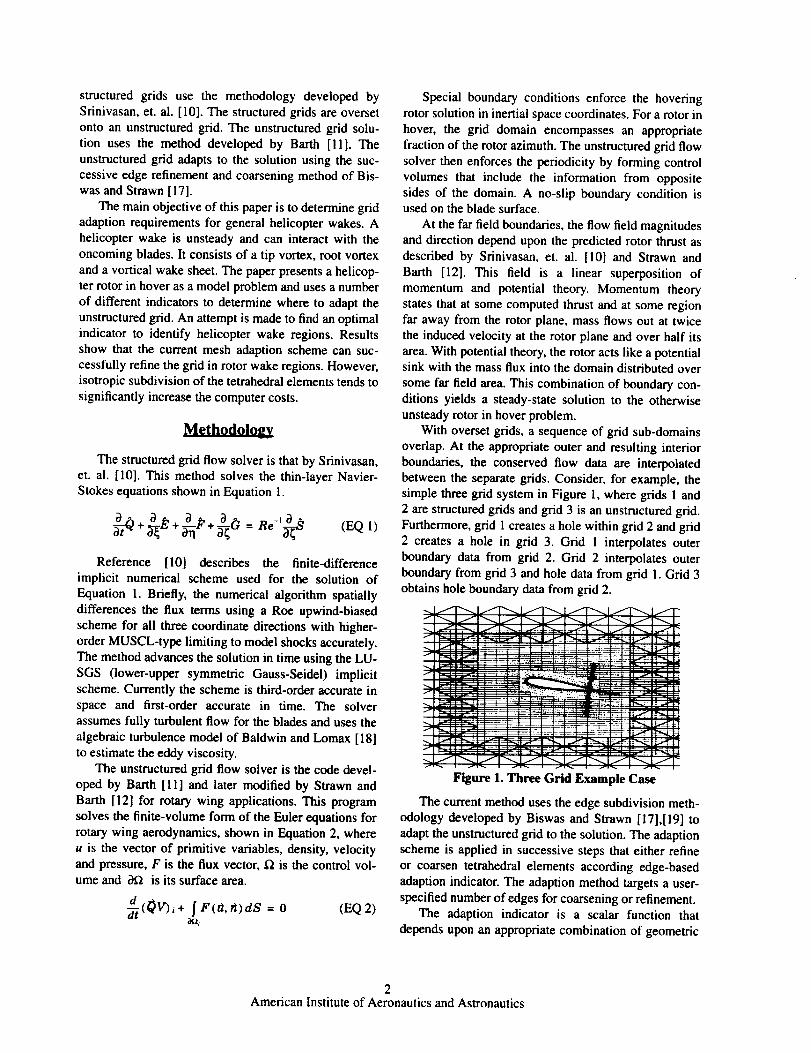
With overset grids, a sequence of grid sub-domains

overlap. At the appropriate outer and resulting interior

boundaries, the conserved flow data are interpolated

between the separate grids. Consider, for example, the

simple three grid system in Figure 1, where grids 1 and

2 are structured grids and grid 3 is an unstructured grid.

Furthermore, grid 1 creates a hole within grid 2 and grid2 creates a hole in grid 3. Grid 1 interpolates outer

boundary data from grid 2. Grid 2 interpolates outer

boundary from grid 3 and hole data from grid 1. Grid 3

obtains hole boundary data from grid 2.

Figure 1. Three Grid Example Case

The current method uses the edge subdivision meth-

odology developed by Biswas and Strawn [17],[19] to

adapt the unstructured grid to the solution. The adaptionscheme is applied in successive steps that either refine

or coarsen tetrahedral elements according edge-basedadaption indicator. The adaption method targets a user-

specified number of edges for coarsening or refinement.

The adaption indicator is a scalar function that

depends upon an appropriate combination of geometric

2American Institute of Aeronautics and Astronautics

andflowfieldinformation.Thispaperusesvorticitymagnitudeasthegeneraladaptionindicator.However,thevorticitymagnitudeis highlynonlinearwithveryhighlevelsatthetipvortexandwakesheet.Scalingthevorticityby theedgelengthbetweentwonodesasshownin Equation3 canalleviateexcessivegridclus-teringatthesehighgradientregions.

indicator (c°J2+ °_jl)Led¢e- 2 (EQ 3)

After each successive refinement step, the flow

solver updates the flow field data and further converges

the solution. However, the computed vorticity magni-tude in the adapted region may further increase, causing

repeated subdivision near the vortex and in the wake

sheet. Excessive refinement can cause poor distribution

of grid points which results in an inefficient use of avail-

able computer memory. Constraining the levels of

refinement helps to more evenly distribute the grid

refinement. In the current work, the grids are allowed to

refine up to a maximum of three subdivision levels.

The helicopter rotor wake is the predominant flow

feature in hover. Further geometric constraints were

imposed to help improve the tip vortex resolution. Thefinal adaption indicator uses a scaled vorticity that

allows the grid to refine to only three levels. The adap-

tion is then limited to occur only within 2 chords of the

blade tip radius.

The rotor solutions in this paper use the structured/

unstructured overset grid system reported earlier by

Duque [20]. This grid system models the rectangular

planform two bladed rotor by Caradonna and Tung [21].

This blade has a NACA0012 cross section, a squared off

tip and an aspect ratio of 6. The overset grid system con-sists of four separate grids - one grid for the main rotor

blade, two grids for the root and the tip and one for the

far field unstructured wake grid. As shown in Figure 2,

the blade grid captures the overall shape of the geometry

under investigation. The grid accurately resolves the

blade tips through the tip cap grid illustrated in Figure 2.

These grids are overset onto an unstructured grid that is

generated by algebraically subdividing an existing

structured grid into tetrahedral elements.

The rotor in hover computations were performed at

one of the subsonic tip hover test condition reported by

Caradonna and Tung [21 ] (Mti p = 0.439, Re = 1.83 mil-lion, 8° Collective). The solutions reported earlier with

this grid system were used as initial solutions to the

adaption cases. Three different adaption indicators

(scaled vorticity, level constraint and geometric con-

straint) were applied. Through adaptive refinement, the

grids were brought to a maximum upper limit in the

total number of elements. This upper limit gives a good

comparison of the effect of each adaption indicator for a

given amount of computational resources.

Results and Discussion

In the following calculations, the unstructured gridwas limited to a maximum of 1.3 million tetrahedral ele-

ments, 1.5 million edges, or 230,000 nodes. A maxi-

mum of seven refinement/coarsening steps was

implemented. Each grid refinement/coarsening step

required approximately 300 CPU seconds and a maxi-

mum of 96MW of memory on a Cray C-90. Between

each refinement step, the unstructured-grid flow solver

was run for 250 iterations or 2400 single CPU secondsto converge the solution. The combined structured/

unstructured flow solver required a maximum of 32MW

of in-core memory on a Cray C-90.

The discussion gives a progressive comparison of

the adapted grids along different cross sections of the

unstructured grid. The results show that one must care-

fully choose and apply the adaption indicator for effi-

cient use of available computational resources. All of

the indicators based on vorticity demonstrate the ability

to adapt to the tip vortex, root vortex, and wake sheet.However, the relative resolution of these flow features is

highly dependent on the specifics of the adaption indica-

tor. We assume that the most important flow features in

the rotor wake are the tip vortices.

One problem with tetrahedral meshes is that it is

very difficult to subdivide the grid in a truly anisotropic

manner. Isotropic subdivision rapidly leads to high com-

putational costs and the results will show that tetrahe-

dral meshes may not be the ideal unstructured grid

element for helicopter wakes. This is because the pre-

dominate features in helicopter wakes are tip vortices,which are inherently anisotropic. Hexahedral, or mixed-

element meshes are much better suited for anisotropic

subdivision than their tetrahedral counterparts but these

were not used in the present study.

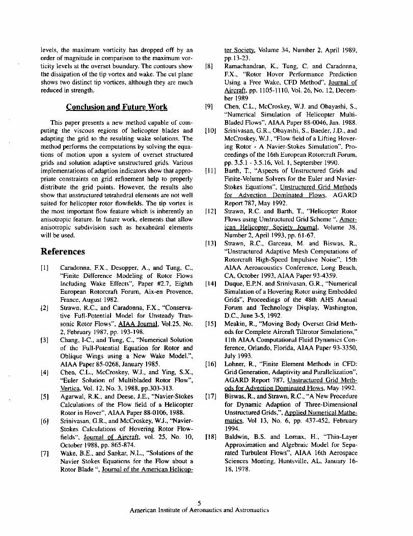
Figure 3 illustrates the grid for the initial and each of

the adapted grids at the periodic plane 90 ° behind the

blade trailing edge. For comparison, Figure 3a shows

the initial coarse grid. Figure 3b shows the final grid

obtained using the scaled vorticity grid indicator. The

grid shows refinement at the tip vortex region asdenoted. In this region, the grid shows multiple levels of

grid refinement. Grid refinement at the root vortex loca-tion is also seen.

Figure 3c shows the grid at the same location butwith a maximum limit of three refinement levels. Four

flow features become evident - initial tip vortex, wake

sheet, root vortex and first passage of tip vortex. Themajor differences between this adapted grid and the pre-

vious are the increased adaption on the wake sheet and


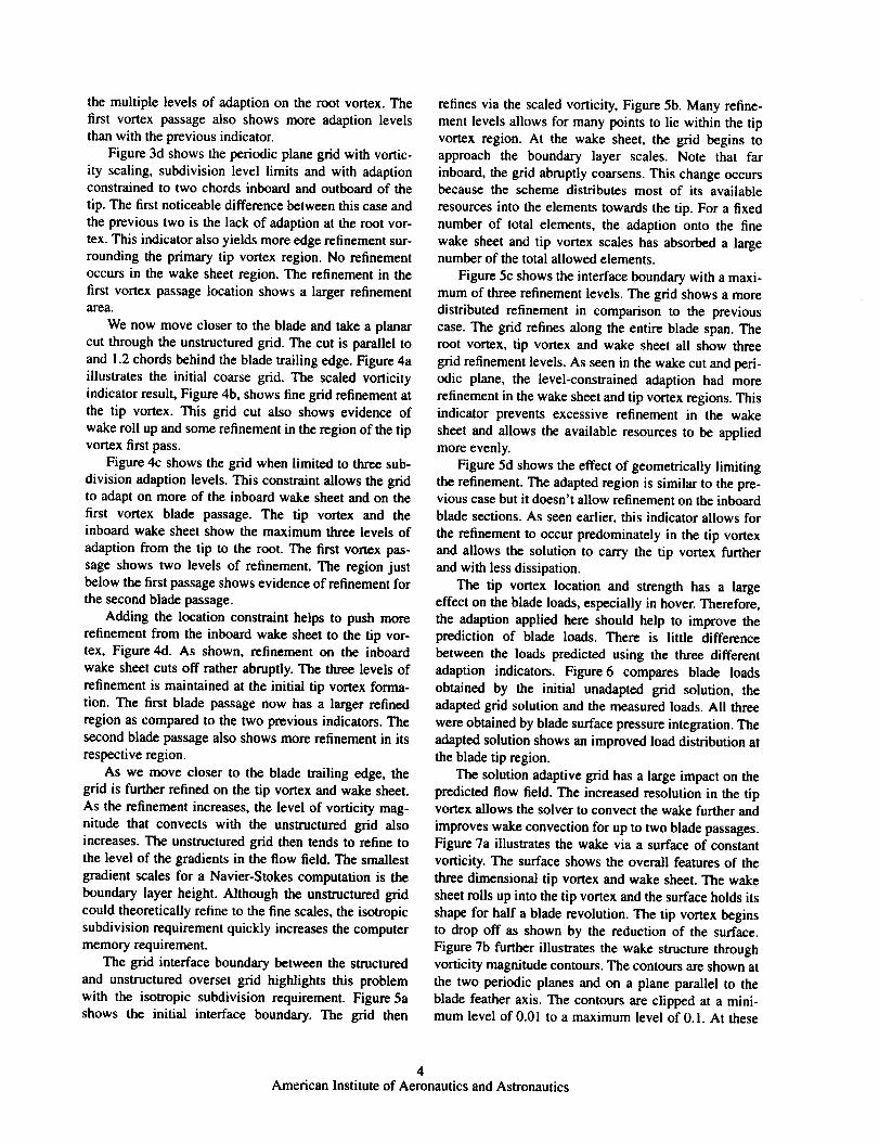
themultiple levels of adaption on the root vortex. The

first vortex passage also shows more adaption levels

than with the previous indicator.Figure 3d shows the periodic plane grid with vortic-

ity scaling, subdivision level limits and with adaptionconstrained to two chords inboard and outboard of the

tip. The first noticeable difference between this case and

the previous two is the lack of adaption at the root vor-

tex. This indicator also yields more edge refinement sur-

rounding the primary tip vortex region. No refinementoccurs in the wake sheet region. The refinement in the

first vortex passage location shows a larger refinement

ar_a.

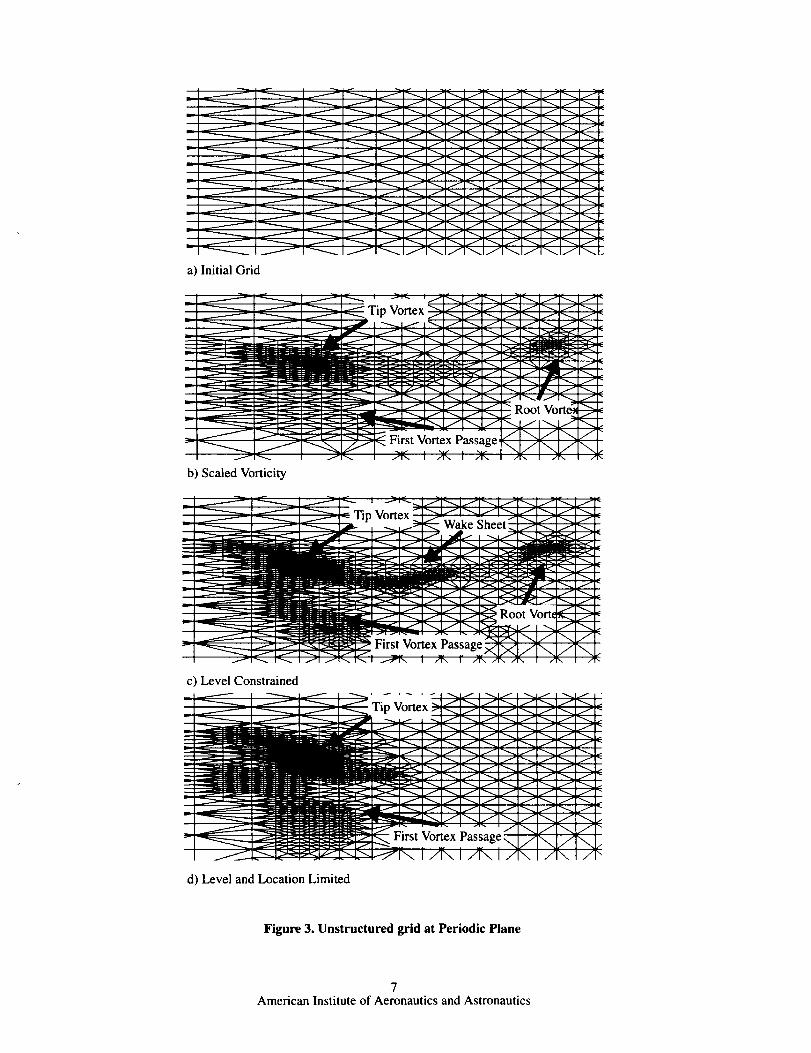
We now move closer to the blade and take a planar

cut through the unstructured grid. The cut is parallel to

and 1.2 chords behind the blade trailing edge. Figure 4a

illustrates the initial coarse grid. The scaled vorticity

indicator result, Figure 4b, shows fine grid refinement at

the tip vortex. This grid cut also shows evidence of

wake roll up and some refinement in the region of the tip

vortex first pass.

Figure 4c shows the grid when limited to three sub-

division adaption levels. This constraint allows the gridto adapt on more of the inboard wake sheet and on the

first vortex blade passage. The tip vortex and theinboard wake sheet show the maximum three levels of

adaption from the tip to the root. The first vortex pas-

sage shows two levels of refinement. The region just

below the first passage shows evidence of refinement for

the second blade passage.

Adding the location constraint helps to push more

refinement from the inboard wake sheet to the tip vor-tex, Figure 4d. As shown, refinement on the inboard

wake sheet cuts off rather abruptly. The three levels of

refinement is maintained at the initial tip vortex forma-

tion. The first blade passage now has a larger refined

region as compared to the two previous indicators. The

second blade passage also shows more refinement in its

respective region.As we move closer to the blade trailing edge, the

grid is further refined on the tip vortex and wake sheet.

As the refinement increases, the level of vorticity mag-

nitude that convects with the unstructured grid also

increases. The unstructured grid then tends to refine to

the level of the gradients in the flow field. The smallest

gradient scales for a Navier-Stokes computation is the

boundary layer height. Although the unstructured grid

could theoretically refine to the fine scales, the isotropic

subdivision requirement quickly increases the computer

memory requirement.

The grid interface boundary between the structured

and unstructured overset grid highlights this problem

with the isotropic subdivision requirement. Figure 5a

shows the initial interface boundary. The grid then

refines via the scaled vorticity, Figure 5b. Many refine-

ment levels allows for many points to lie within the tip

vortex region. At the wake sheet, the grid begins to

approach the boundary layer scales. Note that far

inboard, the grid abruptly coarsens. This change occursbecause the scheme distributes most of its available

resources into the elements towards the tip. For a fixed

number of total elements, the adaption onto the fine

wake sheet and tip vortex scales has absorbed a largenumber of the total allowed elements.

Figure 5c shows the interface boundary with a maxi-

mum of three refinement levels. The grid shows a more

distributed refinement in comparison to the previous

case. The grid refines along the entire blade span. The

root vortex, tip vortex and wake sheet all show three

grid refinement levels. As seen in the wake cut and peri-

odic plane, the level-constrained adaption had more

refinement in the wake sheet and tip vortex regions. This

indicator prevents excessive refinement in the wake

sheet and allows the available resources to be applied

more evenly.

Figure 5d shows the effect of geometrically limitingthe refinement. The adapted region is similar to the pre-vious case but it doesn't allow refinement on the inboard

blade sections. As seen earlier, this indicator allows for

the refinement to occur predominately in the tip vortex

and allows the solution to carry the tip vortex further

and with less dissipation.

The tip vortex location and strength has a large

effect on the blade loads, especially in hover. Therefore,

the adaption applied here should help to improve theprediction of blade loads. There is little difference

between the loads predicted using the three different

adaption indicators. Figure6 compares blade loads

obtained by the initial unadapted grid solution, the

adapted grid solution and the measured loads. All three

were obtained by blade surface pressure integration. The

adapted solution shows an improved load distribution at

the blade tip region.

The solution adaptive grid has a large impact on the

predicted flow field. The increased resolution in the tipvortex allows the solver to convect the wake further and

improves wake convection for up to two blade passages.

Figure 7a illustrates the wake via a surface of constant

vorticity. The surface shows the overall features of the

three dimensional tip vortex and wake sheet. The wake

sheet rolls up into the tip vortex and the surface holds its

shape for half a blade revolution. The tip vortex begins

to drop off as shown by the reduction of the surface.

Figure 7b further illustrates the wake structure through

vorticity magnitude contours. The contours are shown at

the two periodic planes and on a plane parallel to the

blade feather axis. The contours are clipped at a mini-mum level of 0.01 to a maximum level of 0.1. At these


levels,themaximumvorticityhasdroppedoff byanorderofmagnitudeincomparisontothemaximumvor-ticitylevelsattheoversetboundary.Thecontoursshowthedissipationofthetipvortexandwake.Thecutplaneshowstwodistincttipvortices,althoughtheyaremuchreducedinstrength.

Conclusion and Future Work

This paper presents a new method capable of com-

puting the viscous regions of helicopter blades and

adapting the grid to the resulting wake solutions. Themethod performs the computations by solving the equa-

tions of motion upon a system of overset structured

grids and solution adaptive unstructured grids. Various

implementations of adaption indicators show that appro-

priate constraints on grid refinement help to properly

distribute the grid points. However, the results alsoshow that unstructured tetrahedral elements are not well

suited for helicopter rotor flowfields. The tip vortex is

the most important flow feature which is inherently an

anisotropic feature. In future work, elements that allow

anisotropic subdivision such as hexahedral elementswill be used.

References

[1]

[2]

[31

[41

[51

[6]

[7]

Caradonna, EX., Desopper, A., and Tung, C.,

"Finite Difference Modeling of Rotor Flows

Including Wake Effects", Paper #2.7, Eighth

European Rotorcraft Forum, Aix-en Provence,

France, August 1982.Strawn, R.C., and Caradonna, EX., "Conserva-

tive Full-Potential Model for Unsteady Tran-

sonic Rotor Flows", AIAA Journal, Vol.25, No.

2, February 1987, pp. 193-198.

Chang, I-C., and Tung, C., "Numerical Solution

of the Full-Potential Equation for Rotor and

Oblique Wings using a New Wake Model.",

AIAA Paper 85-0268, January 1985.

Chen, C.L., McCroskey, W.J., and Ying, S.X.,"Euler Solution of Multibladed Rotor Flow",

Vertica, Vol. 12, No. 3, 1988, pp.303-313.

Agarwal, R.K., and Deese, J.E., "Navier-Stokes

Calculations of the Flow field of a Helicopter

Rotor in Hover", AIAA Paper 88-0106, 1988.

Srinivasan, G.R., and McCroskey, W.J., "Navier-

Stokes Calculations of Hovering Rotor Flow-

fields", Journal of Aircraft, vol. 25, No. 10,

October 1988, pp. 865-874.Wake, B.E., and Sankar, N.L., "Solutions of the

Navier Stokes Equations for the Flow about a

Rotor Blade ", Journal of the American Helicop-

ter Society, Volume 34, Number 2, April 1989,

pp. 13-23.

[8] Ramachandran, K., Tung, C. and Caradonna,EX., "Rotor Hover Performance Prediction

Using a Free Wake, CFD Method", Journal of

Aircraft, pp. 1105-1110, Vol. 26, No. 12, Decem-ber 1989

[9] Chen, C.L., McCroskey, W.J. and Obayashi, S.,

"Numerical Simulation of Helicopter Multi-

Bladed Flows", AIAA Paper 88-0046, Jan. 1988.

[10] Srinivasan, G.R., Obayashi, S., Baeder, J.D., and

McCroskey, W.J., "Flow field of a Lifting Hover-ing Rotor - A Navier-Stokes Simulation", Pro-

ceedings of the 16th European Rotorcraft Forum,

pp. 3.5.1 - 3.5.16, Vol. 1, September 1990.

[11] Barth, T., "Aspects of Unstructured Grids andFinite-Volume Solvers for the Euler and Navier-

Stokes Equations", Unstructured Grid Methodsfor Advection Dominated Flows, AGARD

Report 787, May 1992.

[12] Strawn, R.C. and Barth, T., "Helicopter Rotor

Flows using Unstructured Grid Scheme ", Amer-

ican Helicopter Society Journal, Volume 38,Number 2, April 1993, pp. 61-67.

[131 Strawn, R.C., Garceau, M. and Biswas, R.,

"Unstructured Adaptive Mesh Computations of

Rotorcraft High-Speed Impulsive Noise", 15th

A1AA Aeroacoustics Conference, Long Beach,

CA, October 1993, AIAA Paper 93-4359.

[14] Duque, E.P.N. and Srinivasan, G.R., "Numerical

Simulation of a Hovering Rotor using EmbeddedGrids", Proceedings of the 48th AHS Annual

Forum and Technology Display, Washington,D.C., June 3-5, 1992.

[15] Meakin, R., "Moving Body Overset Grid Meth-

ods for Complete Aircraft Tiltrotor Simulations,"

1lth AIAA Computational Fluid Dynamics Con-

ference, Orlando, Florida, AIAA Paper 93-3350,

July 1993.[16] Lohner, R., "Finite Element Methods in CFD:

Grid Generation, Adaptivity and Parallelization",

AGARD Report 787, Unstructured Grid Meth-

ods for Advection Dominated Flows, May 1992.

[17] Biswas, R., and Strawn, R.C., "A New Procedure

for Dynamic Adaption of Three-Dimensional

Unstructured Grids,", Applied Numerical Mathe-

matics, Vol 13, No. 6, pp. 437-452, February1994.

[18] Baldwin, B.S. and Lomax, H., "Thin-Layer

Approximation and Algebraic Model for Sepa-

rated Turbulent Flows", AIAA 16th Aerospace

Sciences Meeting, Huntsville, AL, January 16-18, 1978.


[19] Biswas, R., and Strawn, R.C., "Dynamic Mesh

Adaption for Tetrahedral Grids," Presented at the14th International Conference on Numerical

Methods in Fluid Dynamics, Bangalore, India,July 11-15, 1994.

[20] Duque, E.P.N., "A Structured/Unstructured

Embedded Grid Solver for Helicopter Rotor

Flows", AHS 50th Annual Forum, Washington

D.C., May 11-13, 1994.

[21] Caradonna, F.X. and Tung, C., "Experimental

and Analytical Studies of a Model Helicopter

Rotor in Hover", NASA TM-81232, September1981.

Blade Grid Tip Cap and Root Cap Grid

Unstructured Background Wake Grid

Figure 2: Rotor Grid Systems


m

/ _/_i/_/

..__ _ _/ _ .,_fl"_-_ / __- / _/_1/ _/

lilt v'-..

a) Initial Grid

el

V--

b) Scaled Vorticity

c) Level Constrained

d) Level and Location Limited

/

,___.___

i\f

Figure 3. Unstructured grid at Periodic Plane


,'Ix/"v '" ,,/\L 1\ / ,,/!\/",,v\,_/_/r d/\ / \,/\

/IX /IX /\ I /\ /I\ I AX I _\ ,

a) Initial b) Scaled Vorticity

I-_ _ fl

.... --y.7_- _ __ _ -_ -

_1._ _ f'_ _ "-_

,-p.a/

%

_-'_.S_l_ /,_- ..._11_-__/--_"7_1/ _ I-"-

- -_l/_li t" _

• / /\

c) Level Constrained d) Level and Location Constrained

Figure 4. Unstructured grid at 1.2 Chords Behind Trailing Edge


a)Initial

b)ScaledVorticity

c)LevelConstrained

d) Level and Location Constrained

Figure 5. Structured/Unstructured Grid Interface Boundarye

Lift

0.4-

0.3-

0.2-

0.1-

0.00.0

Adapted L

.... Initial J

• Experiment

0.2 0.4 0.6 0.8

r/R

Figure 6. Spanwise Loading with Adapted and InitialUnstructured Wake Grid

1.0


a) Isosurface of Voricity = 0.03

Tip Vortex at RearPeriodic Plane

Rotor Blade

( Trailing Edge )

b) Vorticity Contours ( min = 0.01, max = 0.1 )

Tip Vortex at FrontPeriodic Plane

1st Blade Passage

2nd Blade Passage

Figure 7. Isosurface of Vorticity and Vorticity ContoursLevel and Geometry Limited Unstructured Adapted Grid


RIACSMail Stop T041-5

NASA Ames Research Center

Moffett Field, CA 94035

Documents

A Solution Adaptive Structured/Unstructured Overset Grid ... · PDF fileA Solution Adaptive Structured/Unstructured Overset Grid ... A SOLUTION ADAPTIVE STRUCTURED/UNSTRUCTURED OVERSET