Embed Size (px)
Citation preview
Introduction Adaptive LBM Realistic computations Conclusions
A block-structured parallel adaptive Lattice-Boltzmannmethod for rotating geometries
Ralf Deiterding∗ & Stephen Wood+
∗Deutsches Zentrum fur Luft- und RaumfahrtBunsenstr. 10, Gottingen, Germany
E-mail: [email protected]
+University of Tennessee - KnoxvilleThe Bredesen Center, Knoxville, TN 37996
SIAM Conference on Parallel Processing for Scientific ComputingFebruary 19, 2014
R. Deiterding, S. Wood – A block-structured adaptive LBM 1
Introduction Adaptive LBM Realistic computations Conclusions
Outline
IntroductionAMROC software
Adaptive LBMLattice Boltzmann methodStructured adaptive mesh refinementVerificationPerformance assessmentComplex geometry consideration
Realistic computationsStatic geometriesSimulation of wind turbines
ConclusionsThings to address
S. Wood was partially sponsored by TN-Score and the Oak Ridge National Laboratory, which is managed by UT-Battelle, LLC underContract No. DE-AC05-00OR22725.
R. Deiterding, S. Wood – A block-structured adaptive LBM 2
Introduction Adaptive LBM Realistic computations Conclusions
AMROC software
AMROC
I Cartesian adaptive fluid solver framework for explicit finite volumemethods. Implements for instance Berger-Collela-type AMR.
I Many shock-capturing methods (MUSCL, (hybrid) WENO, etc.)implemented for complex flux functions.
I Used to drive Virtual Test Facility (VTF) FSI software.
I Targets strongly driven problems (shocks, blast, detonations)
I Geometry embedding via ghost fluid techniques and level set functions.Distance computation with CPT algorithm [Mauch, 2000].
I ∼ 430, 000 LOC in C++, C, Fortran-77, Fortran-90.
I Version V2.0 at http://www.cacr.caltech.edu/asc. V1.1 (no complexboundaries) still at http://amroc.sourceforge.net.
I Version used here V3.0 with significantly enhanced parallelization (V2.1not released).
I Papers: [Deiterding, 2011, Deiterding and Wood, 2013,Deiterding et al., 2009, Deiterding et al., 2007, Deiterding et al., 2006]and at http://www.rdeiterding.de
R. Deiterding, S. Wood – A block-structured adaptive LBM 3
Introduction Adaptive LBM Realistic computations Conclusions
Lattice Boltzmann method
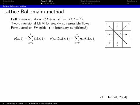
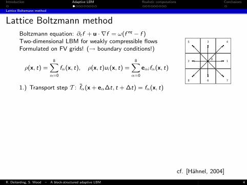
Lattice Boltzmann methodBoltzmann equation: ∂t f + u · ∇f = ω(f eq − f )Two-dimensional LBM for weakly compressible flowsFormulated on FV grids! (→ boundary conditions!)
ρ(x, t) =8Xα=0
fα(x, t), ρ(x, t)ui (x, t) =8Xα=0
eαi fα(x, t)
1.) Transport step T : fα(x + eα∆t, t + ∆t) = fα(x, t)
b
b
b
b
b bb
b
b
3
0
4
1
768
2
5
2.) Collision step C:
fα(·, t + ∆t) = fα(·, t + ∆t) + ω∆t“f eqα (·, t + ∆t)− fα(·, t + ∆t)
”with equilibrium function
f eqα (ρ, u) = ρtα
»1 +
eαu
c2s
+(eαu)2
2c4s− u2
2c4s
–mit tα = 1
9
˘4, 1, 1, 1, 1
4, 1
4, 1, 1
4, 1
4
¯Lattice speed of sound: cs = 1√
3
∆x∆t
, pressure p =Pα f eqα c2
s = ρc2s = ρRT
Collision frequency vs. kinematic viscosity: ω =c2
sν+∆tc2
s /2
cf. [Hahnel, 2004]
R. Deiterding, S. Wood – A block-structured adaptive LBM 4
Introduction Adaptive LBM Realistic computations Conclusions
Lattice Boltzmann method
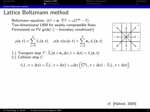
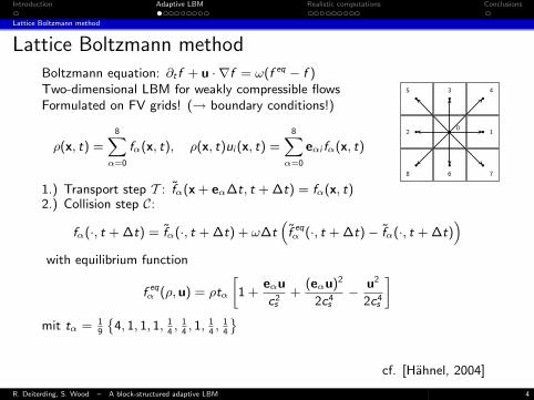
Lattice Boltzmann methodBoltzmann equation: ∂t f + u · ∇f = ω(f eq − f )Two-dimensional LBM for weakly compressible flowsFormulated on FV grids! (→ boundary conditions!)
ρ(x, t) =8Xα=0
fα(x, t), ρ(x, t)ui (x, t) =8Xα=0
eαi fα(x, t)
1.) Transport step T : fα(x + eα∆t, t + ∆t) = fα(x, t)
b
b
b
b
b bb
b
b
3
0
4
1
768
2
5
2.) Collision step C:
fα(·, t + ∆t) = fα(·, t + ∆t) + ω∆t“f eqα (·, t + ∆t)− fα(·, t + ∆t)
”
with equilibrium function
f eqα (ρ, u) = ρtα
»1 +
eαu
c2s
+(eαu)2
2c4s− u2
2c4s
–mit tα = 1
9
˘4, 1, 1, 1, 1
4, 1
4, 1, 1
4, 1
4
¯Lattice speed of sound: cs = 1√
3
∆x∆t
, pressure p =Pα f eqα c2
s = ρc2s = ρRT
Collision frequency vs. kinematic viscosity: ω =c2
sν+∆tc2
s /2
cf. [Hahnel, 2004]
R. Deiterding, S. Wood – A block-structured adaptive LBM 4
Introduction Adaptive LBM Realistic computations Conclusions
Lattice Boltzmann method
Lattice Boltzmann methodBoltzmann equation: ∂t f + u · ∇f = ω(f eq − f )Two-dimensional LBM for weakly compressible flowsFormulated on FV grids! (→ boundary conditions!)
ρ(x, t) =8Xα=0
fα(x, t), ρ(x, t)ui (x, t) =8Xα=0
eαi fα(x, t)
1.) Transport step T : fα(x + eα∆t, t + ∆t) = fα(x, t)
b
b
b
b
b bb
b
b
3
0
4
1
768
2
5
2.) Collision step C:
fα(·, t + ∆t) = fα(·, t + ∆t) + ω∆t“f eqα (·, t + ∆t)− fα(·, t + ∆t)
”with equilibrium function
f eqα (ρ, u) = ρtα
»1 +
eαu
c2s
+(eαu)2
2c4s− u2
2c4s
–mit tα = 1
9
˘4, 1, 1, 1, 1
4, 1
4, 1, 1
4, 1
4
¯
Lattice speed of sound: cs = 1√3
∆x∆t
, pressure p =Pα f eqα c2
s = ρc2s = ρRT
Collision frequency vs. kinematic viscosity: ω =c2
sν+∆tc2
s /2
cf. [Hahnel, 2004]
R. Deiterding, S. Wood – A block-structured adaptive LBM 4
Introduction Adaptive LBM Realistic computations Conclusions
Lattice Boltzmann method
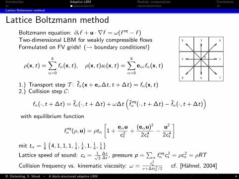
Lattice Boltzmann methodBoltzmann equation: ∂t f + u · ∇f = ω(f eq − f )Two-dimensional LBM for weakly compressible flowsFormulated on FV grids! (→ boundary conditions!)
ρ(x, t) =8Xα=0
fα(x, t), ρ(x, t)ui (x, t) =8Xα=0
eαi fα(x, t)
1.) Transport step T : fα(x + eα∆t, t + ∆t) = fα(x, t)
b
b
b
b
b bb
b
b
3
0
4
1
768
2
5
2.) Collision step C:
fα(·, t + ∆t) = fα(·, t + ∆t) + ω∆t“f eqα (·, t + ∆t)− fα(·, t + ∆t)
”with equilibrium function
f eqα (ρ, u) = ρtα
»1 +
eαu
c2s
+(eαu)2
2c4s− u2
2c4s
–mit tα = 1
9
˘4, 1, 1, 1, 1
4, 1
4, 1, 1
4, 1
4
¯Lattice speed of sound: cs = 1√
3
∆x∆t
, pressure p =Pα f eqα c2
s = ρc2s = ρRT
Collision frequency vs. kinematic viscosity: ω =c2
sν+∆tc2
s /2cf. [Hahnel, 2004]
R. Deiterding, S. Wood – A block-structured adaptive LBM 4
Introduction Adaptive LBM Realistic computations Conclusions
Structured adaptive mesh refinement
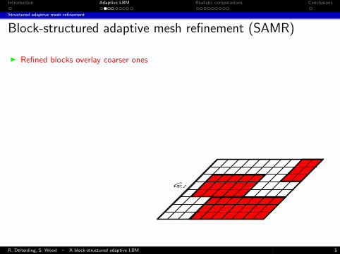
Block-structured adaptive mesh refinement (SAMR)
I Refined blocks overlay coarser ones
I Recursive refinement in space and timeby factor rl [Berger and Colella, 1988]ideal for LBM
I Block (aka patch) based datastructures
+ Numerical scheme only for single patchnecessary
+ Most efficient LBM implementationwith patch-wise for-loops
+ Cache efficient
I Spatial interpolation and averagingcan be used unaltered
- Cluster-algorithm necessary
G2,1
G2,2
G1,1
G1,2
G1,3
G0,1
R. Deiterding, S. Wood – A block-structured adaptive LBM 5
Introduction Adaptive LBM Realistic computations Conclusions
Structured adaptive mesh refinement
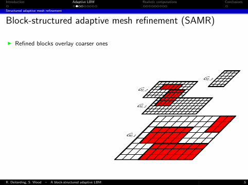
Block-structured adaptive mesh refinement (SAMR)
I Refined blocks overlay coarser ones
I Recursive refinement in space and timeby factor rl [Berger and Colella, 1988]ideal for LBM
I Block (aka patch) based datastructures
+ Numerical scheme only for single patchnecessary
+ Most efficient LBM implementationwith patch-wise for-loops
+ Cache efficient
I Spatial interpolation and averagingcan be used unaltered
- Cluster-algorithm necessary
G2,1
G2,2
G1,1
G1,2
G1,3
G0,1
R. Deiterding, S. Wood – A block-structured adaptive LBM 5

Introduction Adaptive LBM Realistic computations Conclusions
Structured adaptive mesh refinement
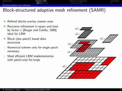
Block-structured adaptive mesh refinement (SAMR)
I Refined blocks overlay coarser ones
I Recursive refinement in space and timeby factor rl [Berger and Colella, 1988]ideal for LBM
I Block (aka patch) based datastructures
+ Numerical scheme only for single patchnecessary
+ Most efficient LBM implementationwith patch-wise for-loops
+ Cache efficient
I Spatial interpolation and averagingcan be used unaltered
- Cluster-algorithm necessary
G2,1
G2,2
G1,1
G1,2
G1,3
G0,1
R. Deiterding, S. Wood – A block-structured adaptive LBM 5

Introduction Adaptive LBM Realistic computations Conclusions
Structured adaptive mesh refinement
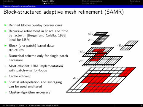
Block-structured adaptive mesh refinement (SAMR)
I Refined blocks overlay coarser ones
I Recursive refinement in space and timeby factor rl [Berger and Colella, 1988]ideal for LBM
I Block (aka patch) based datastructures
+ Numerical scheme only for single patchnecessary
+ Most efficient LBM implementationwith patch-wise for-loops
+ Cache efficient
I Spatial interpolation and averagingcan be used unaltered
- Cluster-algorithm necessary
G2,1
G2,2
G1,1
G1,2
G1,3
G0,1
R. Deiterding, S. Wood – A block-structured adaptive LBM 5
Introduction Adaptive LBM Realistic computations Conclusions
Structured adaptive mesh refinement
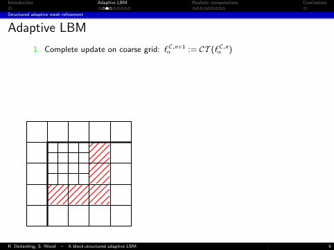
Adaptive LBM
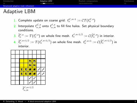
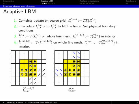
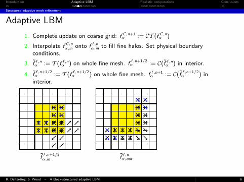
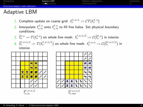
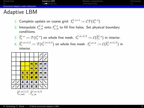
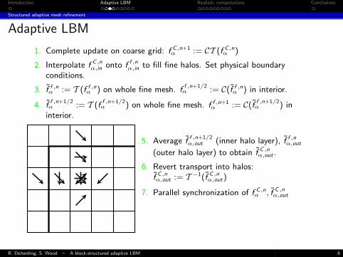
1. Complete update on coarse grid: f C ,n+1α := CT (f C ,n
α )
2. Interpolate f C ,nα,in onto f f ,n
α,in to fill fine halos. Set physical boundaryconditions.
3. f f ,nα := T (f f ,n
α ) on whole fine mesh. ff ,n+1/2α := C(f f ,n
α ) in interior.
4. ff ,n+1/2α := T (f
f ,n+1/2α ) on whole fine mesh. f f ,n+1
α := C(ff ,n+1/2α ) in
interior.
R. Deiterding, S. Wood – A block-structured adaptive LBM 6
Introduction Adaptive LBM Realistic computations Conclusions
Structured adaptive mesh refinement
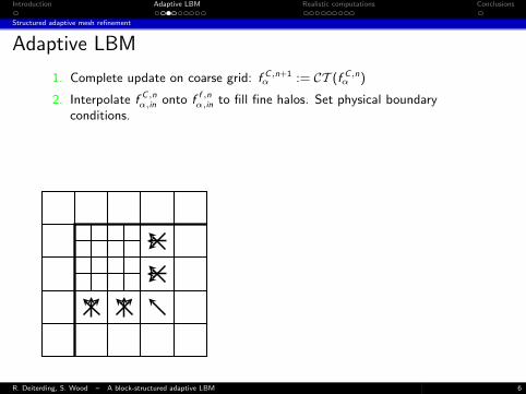
Adaptive LBM
1. Complete update on coarse grid: f C ,n+1α := CT (f C ,n
α )
2. Interpolate f C ,nα,in onto f f ,n
α,in to fill fine halos. Set physical boundaryconditions.
3. f f ,nα := T (f f ,n
α ) on whole fine mesh. ff ,n+1/2α := C(f f ,n
α ) in interior.
4. ff ,n+1/2α := T (f
f ,n+1/2α ) on whole fine mesh. f f ,n+1
α := C(ff ,n+1/2α ) in
interior.
R. Deiterding, S. Wood – A block-structured adaptive LBM 6
Introduction Adaptive LBM Realistic computations Conclusions
Structured adaptive mesh refinement
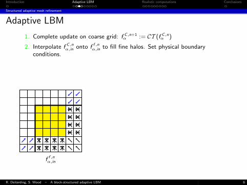
Adaptive LBM
1. Complete update on coarse grid: f C ,n+1α := CT (f C ,n
α )
2. Interpolate f C ,nα,in onto f f ,n
α,in to fill fine halos. Set physical boundaryconditions.
3. f f ,nα := T (f f ,n
α ) on whole fine mesh. ff ,n+1/2α := C(f f ,n
α ) in interior.
4. ff ,n+1/2α := T (f
f ,n+1/2α ) on whole fine mesh. f f ,n+1
α := C(ff ,n+1/2α ) in
interior.
f f ,nα,in
R. Deiterding, S. Wood – A block-structured adaptive LBM 6
Introduction Adaptive LBM Realistic computations Conclusions
Structured adaptive mesh refinement
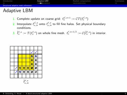
Adaptive LBM
1. Complete update on coarse grid: f C ,n+1α := CT (f C ,n
α )
2. Interpolate f C ,nα,in onto f f ,n
α,in to fill fine halos. Set physical boundaryconditions.
3. f f ,nα := T (f f ,n
α ) on whole fine mesh. ff ,n+1/2α := C(f f ,n
α ) in interior.
4. ff ,n+1/2α := T (f
f ,n+1/2α ) on whole fine mesh. f f ,n+1
α := C(ff ,n+1/2α ) in
interior.
f f ,nα,in
R. Deiterding, S. Wood – A block-structured adaptive LBM 6
Introduction Adaptive LBM Realistic computations Conclusions
Structured adaptive mesh refinement
Adaptive LBM
1. Complete update on coarse grid: f C ,n+1α := CT (f C ,n
α )
2. Interpolate f C ,nα,in onto f f ,n
α,in to fill fine halos. Set physical boundaryconditions.
3. f f ,nα := T (f f ,n
α ) on whole fine mesh. ff ,n+1/2α := C(f f ,n
α ) in interior.
4. ff ,n+1/2α := T (f
f ,n+1/2α ) on whole fine mesh. f f ,n+1
α := C(ff ,n+1/2α ) in
interior.
ff ,n+1/2α,in
R. Deiterding, S. Wood – A block-structured adaptive LBM 6
Introduction Adaptive LBM Realistic computations Conclusions
Structured adaptive mesh refinement
Adaptive LBM
1. Complete update on coarse grid: f C ,n+1α := CT (f C ,n
α )
2. Interpolate f C ,nα,in onto f f ,n
α,in to fill fine halos. Set physical boundaryconditions.
3. f f ,nα := T (f f ,n
α ) on whole fine mesh. ff ,n+1/2α := C(f f ,n
α ) in interior.
4. ff ,n+1/2α := T (f
f ,n+1/2α ) on whole fine mesh. f f ,n+1
α := C(ff ,n+1/2α ) in
interior.
ff ,n+1/2α,in f f ,n
α,out
R. Deiterding, S. Wood – A block-structured adaptive LBM 6
Introduction Adaptive LBM Realistic computations Conclusions
Structured adaptive mesh refinement
Adaptive LBM
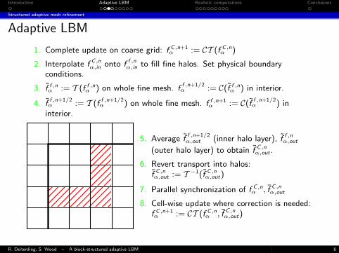
1. Complete update on coarse grid: f C ,n+1α := CT (f C ,n
α )
2. Interpolate f C ,nα,in onto f f ,n
α,in to fill fine halos. Set physical boundaryconditions.
3. f f ,nα := T (f f ,n
α ) on whole fine mesh. ff ,n+1/2α := C(f f ,n
α ) in interior.
4. ff ,n+1/2α := T (f
f ,n+1/2α ) on whole fine mesh. f f ,n+1
α := C(ff ,n+1/2α ) in
interior.
ff ,n+1/2α,in f
f ,n+1/2α,out
R. Deiterding, S. Wood – A block-structured adaptive LBM 6
Introduction Adaptive LBM Realistic computations Conclusions
Structured adaptive mesh refinement
Adaptive LBM
1. Complete update on coarse grid: f C ,n+1α := CT (f C ,n
α )
2. Interpolate f C ,nα,in onto f f ,n
α,in to fill fine halos. Set physical boundaryconditions.
3. f f ,nα := T (f f ,n
α ) on whole fine mesh. ff ,n+1/2α := C(f f ,n
α ) in interior.
4. ff ,n+1/2α := T (f
f ,n+1/2α ) on whole fine mesh. f f ,n+1
α := C(ff ,n+1/2α ) in
interior.
ff ,n+1/2α,out , f
f ,n+1/2α,in
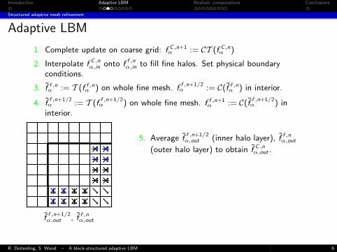
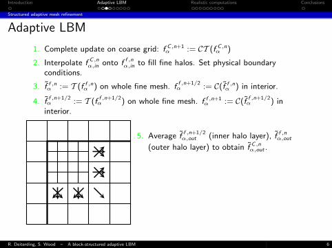
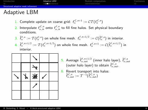
5. Average ff ,n+1/2α,out (inner halo layer), f f ,n
α,out
(outer halo layer) to obtain f C ,nα,out .
6. Revert transport into halos:f C ,nα,out := T −1(f C ,n
α,out)
7. Parallel synchronization of f C ,nα , f C ,n
α,out
8. Cell-wise update where correction is needed:f C ,n+1α := CT (f C ,n
α , f C ,nα,out)
R. Deiterding, S. Wood – A block-structured adaptive LBM 6
Introduction Adaptive LBM Realistic computations Conclusions
Structured adaptive mesh refinement
Adaptive LBM
1. Complete update on coarse grid: f C ,n+1α := CT (f C ,n
α )
2. Interpolate f C ,nα,in onto f f ,n
α,in to fill fine halos. Set physical boundaryconditions.
3. f f ,nα := T (f f ,n
α ) on whole fine mesh. ff ,n+1/2α := C(f f ,n
α ) in interior.
4. ff ,n+1/2α := T (f
f ,n+1/2α ) on whole fine mesh. f f ,n+1
α := C(ff ,n+1/2α ) in
interior.
ff ,n+1/2α,out , f f ,n
α,out
5. Average ff ,n+1/2α,out (inner halo layer), f f ,n
α,out
(outer halo layer) to obtain f C ,nα,out .
6. Revert transport into halos:f C ,nα,out := T −1(f C ,n
α,out)
7. Parallel synchronization of f C ,nα , f C ,n
α,out
8. Cell-wise update where correction is needed:f C ,n+1α := CT (f C ,n
α , f C ,nα,out)
R. Deiterding, S. Wood – A block-structured adaptive LBM 6
Introduction Adaptive LBM Realistic computations Conclusions
Structured adaptive mesh refinement
Adaptive LBM
1. Complete update on coarse grid: f C ,n+1α := CT (f C ,n
α )
2. Interpolate f C ,nα,in onto f f ,n
α,in to fill fine halos. Set physical boundaryconditions.
3. f f ,nα := T (f f ,n
α ) on whole fine mesh. ff ,n+1/2α := C(f f ,n
α ) in interior.
4. ff ,n+1/2α := T (f
f ,n+1/2α ) on whole fine mesh. f f ,n+1
α := C(ff ,n+1/2α ) in
interior.
5. Average ff ,n+1/2α,out (inner halo layer), f f ,n
α,out
(outer halo layer) to obtain f C ,nα,out .
6. Revert transport into halos:f C ,nα,out := T −1(f C ,n
α,out)
7. Parallel synchronization of f C ,nα , f C ,n
α,out
8. Cell-wise update where correction is needed:f C ,n+1α := CT (f C ,n
α , f C ,nα,out)
R. Deiterding, S. Wood – A block-structured adaptive LBM 6
Introduction Adaptive LBM Realistic computations Conclusions
Structured adaptive mesh refinement
Adaptive LBM
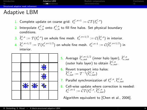
1. Complete update on coarse grid: f C ,n+1α := CT (f C ,n
α )
2. Interpolate f C ,nα,in onto f f ,n
α,in to fill fine halos. Set physical boundaryconditions.
3. f f ,nα := T (f f ,n
α ) on whole fine mesh. ff ,n+1/2α := C(f f ,n
α ) in interior.
4. ff ,n+1/2α := T (f
f ,n+1/2α ) on whole fine mesh. f f ,n+1
α := C(ff ,n+1/2α ) in
interior.
5. Average ff ,n+1/2α,out (inner halo layer), f f ,n
α,out
(outer halo layer) to obtain f C ,nα,out .
6. Revert transport into halos:f C ,nα,out := T −1(f C ,n
α,out)
7. Parallel synchronization of f C ,nα , f C ,n
α,out
8. Cell-wise update where correction is needed:f C ,n+1α := CT (f C ,n
α , f C ,nα,out)
Algorithm equivalent to [Chen et al., 2006].
R. Deiterding, S. Wood – A block-structured adaptive LBM 6
Introduction Adaptive LBM Realistic computations Conclusions
Structured adaptive mesh refinement
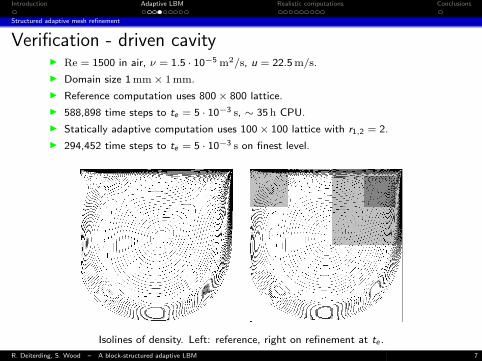
Verification - driven cavityI Re = 1500 in air, ν = 1.5 · 10−5 m2/s, u = 22.5 m/s.
I Domain size 1 mm× 1mm.
I Reference computation uses 800× 800 lattice.
I 588,898 time steps to te = 5 · 10−3 s, ∼ 35 h CPU.
I Statically adaptive computation uses 100× 100 lattice with r1,2 = 2.
I 294,452 time steps to te = 5 · 10−3 s on finest level.
Isolines of density. Left: reference, right on refinement at te .
R. Deiterding, S. Wood – A block-structured adaptive LBM 7
Introduction Adaptive LBM Realistic computations Conclusions
Verification
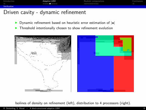
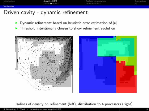
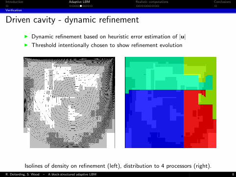
Driven cavity - dynamic refinement
I Dynamic refinement based on heuristic error estimation of |u|I Threshold intentionally chosen to show refinement evolution
Isolines of density on refinement (left), distribution to 4 processors (right).
R. Deiterding, S. Wood – A block-structured adaptive LBM 8
Introduction Adaptive LBM Realistic computations Conclusions
Verification
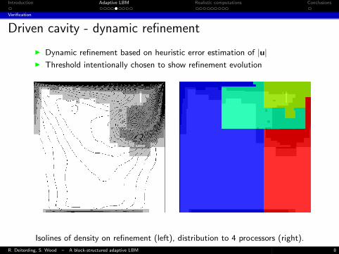
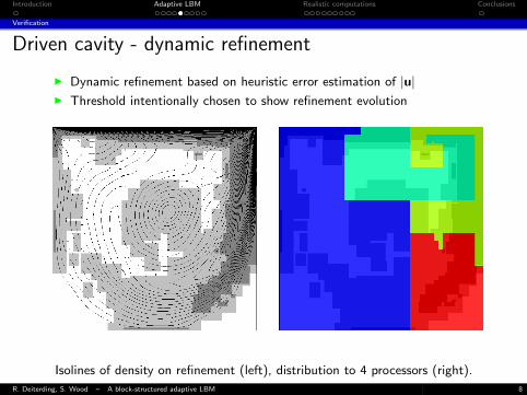
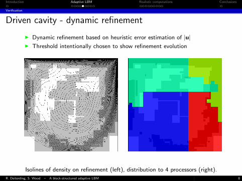
Driven cavity - dynamic refinement
I Dynamic refinement based on heuristic error estimation of |u|I Threshold intentionally chosen to show refinement evolution
Isolines of density on refinement (left), distribution to 4 processors (right).
R. Deiterding, S. Wood – A block-structured adaptive LBM 8
Introduction Adaptive LBM Realistic computations Conclusions
Verification
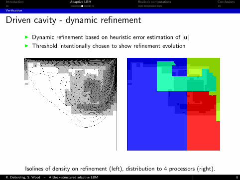
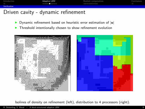
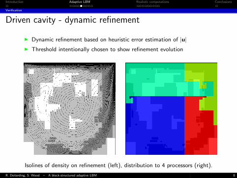
Driven cavity - dynamic refinement
I Dynamic refinement based on heuristic error estimation of |u|I Threshold intentionally chosen to show refinement evolution
Isolines of density on refinement (left), distribution to 4 processors (right).
R. Deiterding, S. Wood – A block-structured adaptive LBM 8
Introduction Adaptive LBM Realistic computations Conclusions
Verification
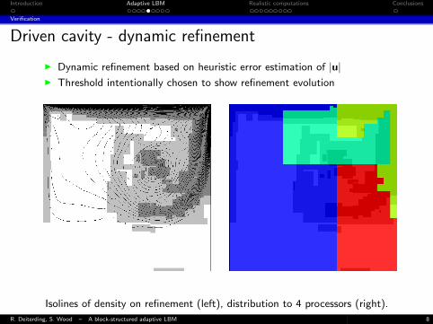
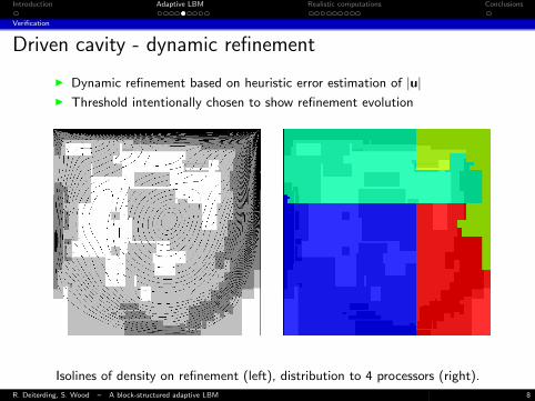
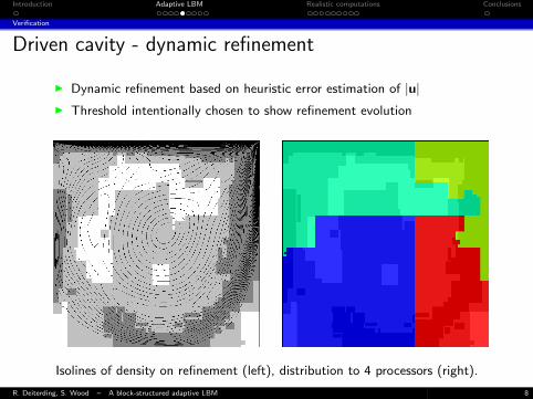
Driven cavity - dynamic refinement
I Dynamic refinement based on heuristic error estimation of |u|I Threshold intentionally chosen to show refinement evolution
Isolines of density on refinement (left), distribution to 4 processors (right).
R. Deiterding, S. Wood – A block-structured adaptive LBM 8
Introduction Adaptive LBM Realistic computations Conclusions
Verification
Driven cavity - dynamic refinement
I Dynamic refinement based on heuristic error estimation of |u|I Threshold intentionally chosen to show refinement evolution
Isolines of density on refinement (left), distribution to 4 processors (right).
R. Deiterding, S. Wood – A block-structured adaptive LBM 8
Introduction Adaptive LBM Realistic computations Conclusions
Performance assessment
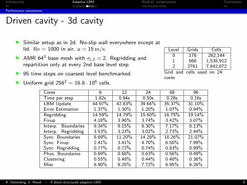
Driven cavity - 3d cavity
I Similar setup as in 2d. No-slip wall everywhere except atlid. Re = 1000 in air, u = 15 m/s.
I AMR 643 base mesh with r1,2 = 2. Regridding andrepartition only at every 2nd base level step.
I 95 time steps on coarsest level benchmarked.
I Uniform grid 2563 = 16.8 · 106 cells.
Level Grids Cells0 178 262,1441 668 1,538,9122 2761 7,842,872
Grid and cells used on 24cores
Cores 6 12 24 48 96Time per step 1.82s 0.94s 0.50s 0.28s 0.16sLBM Update 44.97% 42.83% 39.64% 35.37% 31.10%Error Estimation 1.37% 1.30% 1.20% 1.07% 0.94%Regridding 14.59% 14.79% 15.60% 16.75% 19.14%Fixup 4.18% 3.96% 3.74% 3.42% 3.07%Interp. Boundaries 9.34% 9.15% 8.30% 7.17% 6.13%Interp. Regridding 3.53% 3.23% 3.02% 2.73% 2.44%Sync Boundaries 8.69% 11.20% 14.28% 18.26% 21.07%Sync Fixup 2.41% 3.41% 4.70% 6.50% 7.99%Sync Regridding 0.77% 0.72% 0.74% 0.83% 0.99%Phys. Boundaries 0.69% 0.68% 0.63% 0.56% 0.49%Clustering 0.55% 0.48% 0.44% 0.40% 0.36%Misc 8.90% 8.25% 7.72% 6.95% 6.26%
R. Deiterding, S. Wood – A block-structured adaptive LBM 9
Introduction Adaptive LBM Realistic computations Conclusions
Performance assessment
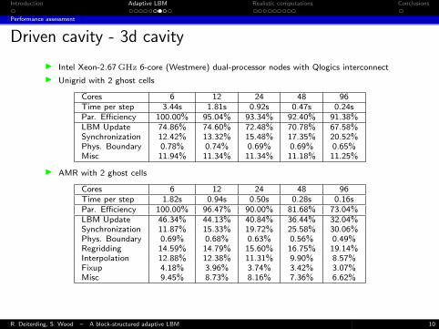
Driven cavity - 3d cavity
I Intel Xeon-2.67 GHz 6-core (Westmere) dual-processor nodes with Qlogics interconnect
I Unigrid with 2 ghost cells
Cores 6 12 24 48 96Time per step 3.44s 1.81s 0.92s 0.47s 0.24sPar. Efficiency 100.00% 95.04% 93.34% 92.40% 91.38%LBM Update 74.86% 74.60% 72.48% 70.78% 67.58%Synchronization 12.42% 13.32% 15.48% 17.35% 20.52%Phys. Boundary 0.78% 0.74% 0.69% 0.69% 0.65%Misc 11.94% 11.34% 11.34% 11.18% 11.25%
I AMR with 2 ghost cells
Cores 6 12 24 48 96Time per step 1.82s 0.94s 0.50s 0.28s 0.16sPar. Efficiency 100.00% 96.47% 90.00% 81.68% 73.04%LBM Update 46.34% 44.13% 40.84% 36.44% 32.04%Synchronization 11.87% 15.33% 19.72% 25.58% 30.06%Phys. Boundary 0.69% 0.68% 0.63% 0.56% 0.49%Regridding 14.59% 14.79% 15.60% 16.75% 19.14%Interpolation 12.88% 12.38% 11.31% 9.90% 8.57%Fixup 4.18% 3.96% 3.74% 3.42% 3.07%Misc 9.45% 8.73% 8.16% 7.36% 6.62%
I Expense for boundary is increased compared to FV methods because the algorithm uses fewfloating point operations but a large state vector!
R. Deiterding, S. Wood – A block-structured adaptive LBM 10
Introduction Adaptive LBM Realistic computations Conclusions
Performance assessment
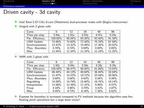
Driven cavity - 3d cavity
I Intel Xeon-2.67 GHz 6-core (Westmere) dual-processor nodes with Qlogics interconnect
I Unigrid with 2 ghost cells
Cores 6 12 24 48 96Time per step 3.44s 1.81s 0.92s 0.47s 0.24sPar. Efficiency 100.00% 95.04% 93.34% 92.40% 91.38%LBM Update 74.86% 74.60% 72.48% 70.78% 67.58%Synchronization 12.42% 13.32% 15.48% 17.35% 20.52%Phys. Boundary 0.78% 0.74% 0.69% 0.69% 0.65%Misc 11.94% 11.34% 11.34% 11.18% 11.25%
I AMR with 2 ghost cells
Cores 6 12 24 48 96Time per step 1.82s 0.94s 0.50s 0.28s 0.16sPar. Efficiency 100.00% 96.47% 90.00% 81.68% 73.04%LBM Update 46.34% 44.13% 40.84% 36.44% 32.04%Synchronization 11.87% 15.33% 19.72% 25.58% 30.06%Phys. Boundary 0.69% 0.68% 0.63% 0.56% 0.49%Regridding 14.59% 14.79% 15.60% 16.75% 19.14%Interpolation 12.88% 12.38% 11.31% 9.90% 8.57%Fixup 4.18% 3.96% 3.74% 3.42% 3.07%Misc 9.45% 8.73% 8.16% 7.36% 6.62%
I Expense for boundary is increased compared to FV methods because the algorithm uses fewfloating point operations but a large state vector!
R. Deiterding, S. Wood – A block-structured adaptive LBM 10
Introduction Adaptive LBM Realistic computations Conclusions
Performance assessment
Driven cavity - 3d cavity
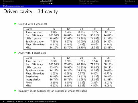
I Unigrid with 1 ghost cell
Cores 6 12 24 48 96Time per step 2.80s 1.46s 0.73s 0.37s 0.18sPar. Efficiency 100.00% 96.09% 95.33% 95.21% 94.82%LBM Update 78.05% 77.08% 75.85% 74.50% 71.38%Synchronization 7.25% 8.67% 10.00% 11.32% 14.35%Phys. Boundary 0.51% 0.46% 0.45% 0.44% 0.44%Misc 14.19% 13.79% 13.70% 13.73% 13.83%
I AMR with 4 ghost cells
Cores 6 12 24 48 96Time per step 3.32s 1.90s 1.21s 0.54s 0.30sPar. Efficiency 100.00% 87.42% 68.76% 77.02% 68.19%LBM Update 43.44% 40.93% 31.33% 34.64% 30.11%Synchronization 14.13% 18.26% 34.73% 25.76% 30.69%Phys. Boundary 1.03% 0.98% 0.77% 0.86% 0.77%Regridding 15.53% 16.02% 13.87% 18.72% 20.82%Interpolation 16.74% 15.71% 11.95% 13.15% 11.51%Fixup 2.89% 2.60% 2.02% 2.28% 2.03%Misc 6.22% 5.50% 5.33% 4.59% 4.08%
I Basically linear dependency on number of ghost cells used
R. Deiterding, S. Wood – A block-structured adaptive LBM 11
Introduction Adaptive LBM Realistic computations Conclusions
Complex geometry consideration
Level-set method for boundary embedding
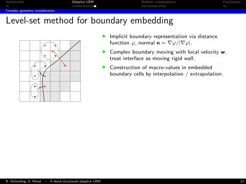
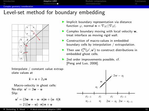
I Implicit boundary representation via distancefunction ϕ, normal n = ∇ϕ/|∇ϕ|.
I Complex boundary moving with local velocity w,treat interface as moving rigid wall.
I Construction of macro-values in embeddedboundary cells by interpolation / extrapolation.
I Then use f eqα (ρ′, u′) to construct distributions in
embedded ghost cells.
I 2nd order improvements possible, cf.[Peng and Luo, 2008].
Interpolate / constant value extrap-olate values at
x = x + 2ϕn
Macro-velocity in ghost cells:No-slip: u′ = 2w − uSlip:
u′ = (2w · n− u · n)n + (u · t)t= 2 ((w − u) · n) n + u
ρj−1 ρj ρj ρj−1
uj−1 uj 2w − uj 2w − uj−1
ut
ut
ut
w
uj
2w − uj
R. Deiterding, S. Wood – A block-structured adaptive LBM 12

Introduction Adaptive LBM Realistic computations Conclusions
Complex geometry consideration
Level-set method for boundary embedding
I Implicit boundary representation via distancefunction ϕ, normal n = ∇ϕ/|∇ϕ|.
I Complex boundary moving with local velocity w,treat interface as moving rigid wall.
I Construction of macro-values in embeddedboundary cells by interpolation / extrapolation.
I Then use f eqα (ρ′, u′) to construct distributions in
embedded ghost cells.
I 2nd order improvements possible, cf.[Peng and Luo, 2008].
Interpolate / constant value extrap-olate values at
x = x + 2ϕn
Macro-velocity in ghost cells:No-slip: u′ = 2w − uSlip:
u′ = (2w · n− u · n)n + (u · t)t= 2 ((w − u) · n) n + u
ρj−1 ρj ρj ρj−1
uj−1 uj 2w − uj 2w − uj−1
ut
ut
ut
w
uj
2w − uj
R. Deiterding, S. Wood – A block-structured adaptive LBM 12
Introduction Adaptive LBM Realistic computations Conclusions
Static geometries
Side-wind investigation for a train model
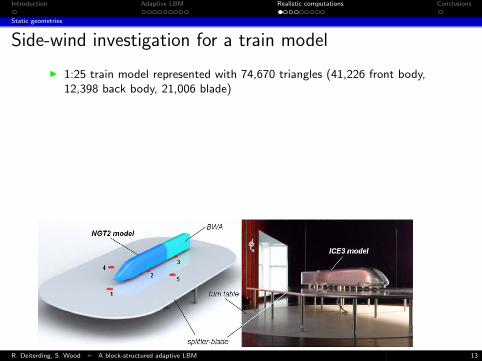
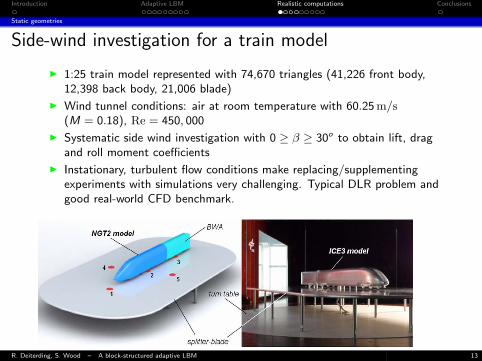
I 1:25 train model represented with 74,670 triangles (41,226 front body,12,398 back body, 21,006 blade)
I Wind tunnel conditions: air at room temperature with 60.25 m/s(M = 0.18), Re = 450, 000
I Systematic side wind investigation with 0 ≥ β ≥ 30o to obtain lift, dragand roll moment coefficients
I Instationary, turbulent flow conditions make replacing/supplementingexperiments with simulations very challenging. Typical DLR problem andgood real-world CFD benchmark.
R. Deiterding, S. Wood – A block-structured adaptive LBM 13
Introduction Adaptive LBM Realistic computations Conclusions
Static geometries
Side-wind investigation for a train model
I 1:25 train model represented with 74,670 triangles (41,226 front body,12,398 back body, 21,006 blade)
I Wind tunnel conditions: air at room temperature with 60.25 m/s(M = 0.18), Re = 450, 000
I Systematic side wind investigation with 0 ≥ β ≥ 30o to obtain lift, dragand roll moment coefficients
I Instationary, turbulent flow conditions make replacing/supplementingexperiments with simulations very challenging. Typical DLR problem andgood real-world CFD benchmark.
R. Deiterding, S. Wood – A block-structured adaptive LBM 13
Introduction Adaptive LBM Realistic computations Conclusions
Static geometries
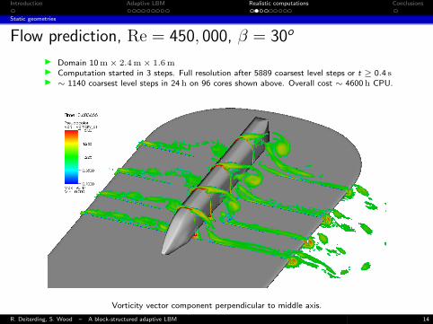
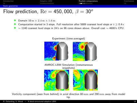
Flow prediction, Re = 450, 000, β = 30o
I Domain 10 m× 2.4 m× 1.6 mI Computation started in 3 steps. Full resolution after 5889 coarsest level steps or t ≥ 0.4 sI ∼ 1140 coarsest level steps in 24 h on 96 cores shown above. Overall cost ∼ 4600 h CPU.
Vorticity vector component perpendicular to middle axis.
R. Deiterding, S. Wood – A block-structured adaptive LBM 14
Introduction Adaptive LBM Realistic computations Conclusions
Static geometries
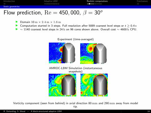
Flow prediction, Re = 450, 000, β = 30o
I Domain 10 m× 2.4 m× 1.6 mI Computation started in 3 steps. Full resolution after 5889 coarsest level steps or t ≥ 0.4 sI ∼ 1140 coarsest level steps in 24 h on 96 cores shown above. Overall cost ∼ 4600 h CPU.
Experiment (time-averaged)
AMROC-LBM Simulation (instantaneoussnapshots)
Vorticity component (seen from behind) in axial direction 80 mm and 290 mm away from modeltip.
R. Deiterding, S. Wood – A block-structured adaptive LBM 14
Introduction Adaptive LBM Realistic computations Conclusions
Static geometries
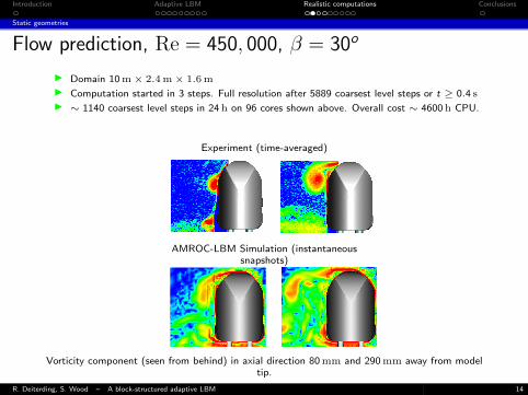
Flow prediction, Re = 450, 000, β = 30o
I Domain 10 m× 2.4 m× 1.6 m
I Computation started in 3 steps. Full resolution after 5889 coarsest level steps or t ≥ 0.4 s
I ∼ 1140 coarsest level steps in 24 h on 96 cores shown above. Overall cost ∼ 4600 h CPU.
Experiment (time-averaged)
AMROC-LBM Simulation (instantaneoussnapshots)
Vorticity component (seen from behind) in axial direction 80 mm and 290 mm away from modeltip.
R. Deiterding, S. Wood – A block-structured adaptive LBM 14
Introduction Adaptive LBM Realistic computations Conclusions
Static geometries
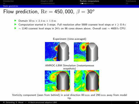
Flow prediction, Re = 450, 000, β = 30o
I Domain 10 m× 2.4 m× 1.6 m
I Computation started in 3 steps. Full resolution after 5889 coarsest level steps or t ≥ 0.4 s
I ∼ 1140 coarsest level steps in 24 h on 96 cores shown above. Overall cost ∼ 4600 h CPU.
Experiment (time-averaged)
AMROC-LBM Simulation (instantaneoussnapshots)
Vorticity component (seen from behind) in axial direction 80 mm and 290 mm away from modeltip.
R. Deiterding, S. Wood – A block-structured adaptive LBM 14
Introduction Adaptive LBM Realistic computations Conclusions
Static geometries
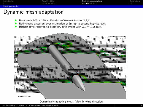
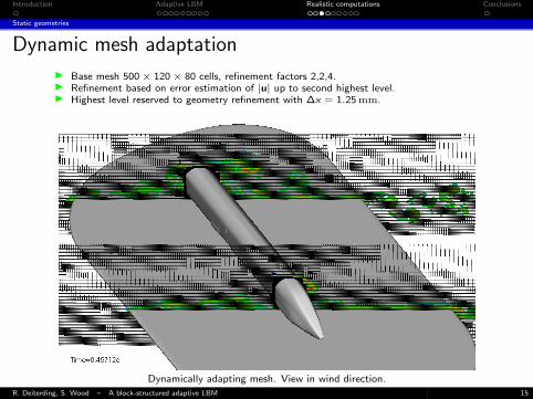
Dynamic mesh adaptation
I Base mesh 500× 120× 80 cells, refinement factors 2,2,4.I Refinement based on error estimation of |u| up to second highest level.I Highest level reserved to geometry refinement with ∆x = 1.25 mm.
Dynamically adapting mesh. View in wind direction.
R. Deiterding, S. Wood – A block-structured adaptive LBM 15
Introduction Adaptive LBM Realistic computations Conclusions
Static geometries
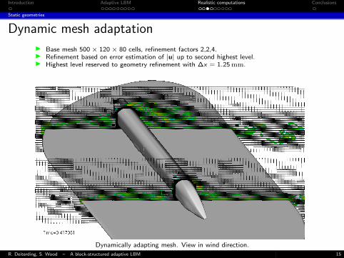
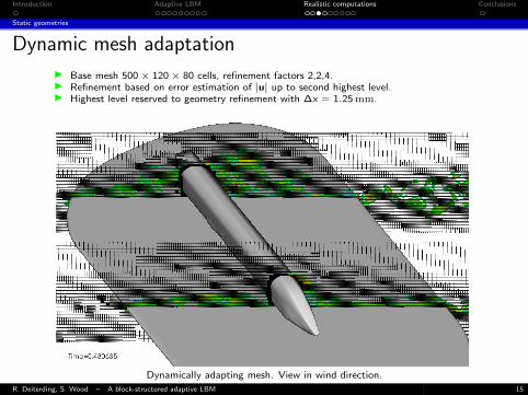
Dynamic mesh adaptation
I Base mesh 500× 120× 80 cells, refinement factors 2,2,4.I Refinement based on error estimation of |u| up to second highest level.I Highest level reserved to geometry refinement with ∆x = 1.25 mm.
Dynamically adapting mesh. View in wind direction.
R. Deiterding, S. Wood – A block-structured adaptive LBM 15

Introduction Adaptive LBM Realistic computations Conclusions
Static geometries
Dynamic mesh adaptation
I Base mesh 500× 120× 80 cells, refinement factors 2,2,4.I Refinement based on error estimation of |u| up to second highest level.I Highest level reserved to geometry refinement with ∆x = 1.25 mm.
Dynamically adapting mesh. View in wind direction.
R. Deiterding, S. Wood – A block-structured adaptive LBM 15
Introduction Adaptive LBM Realistic computations Conclusions
Static geometries
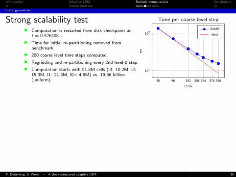
Strong scalability testI Computation is restarted from disk checkpoint at
t = 0.526408 s.
I Time for initial re-partitioning removed frombenchmark.
I 200 coarse level time steps computed.
I Regridding and re-partitioning every 2nd level-0 step.
I Computation starts with 51.8M cells (l3: 10.2M, l2:15.3M, l1: 21.5M, l0= 4.8M) vs. 19.66 billion(uniform).
I Portions for parallel communication quiteconsiderable (4 ghost cells still used).
48 96 192 288 384 576 768
101
102
CPUs
sec
Time per coarse level step
SAMR
Ideal
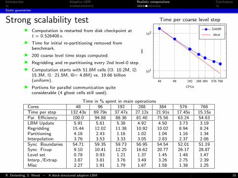
Time in % spent in main operationsCores 48 96 192 288 384 576 768Time per step 132.43s 69.79s 37.47s 27.12s 21.91s 17.45s 15.15sPar. Efficiency 100.0 94.88 88.36 81.40 75.56 63.24 54.63LBM Update 5.91 5.61 5.38 4.92 4.50 3.73 3.19Regridding 15.44 12.02 11.38 10.92 10.02 8.94 8.24Partitioning 4.16 2.43 1.16 1.02 1.04 1.16 1.34Interpolation 3.76 3.53 3.33 3.05 2.83 2.37 2.06Sync Boundaries 54.71 59.35 59.73 56.95 54.54 52.01 51.19Sync Fixup 9.10 10.41 12.25 16.62 20.77 26.17 28.87Level set 0.78 0.93 1.21 1.37 1.45 1.48 1.47Interp./Extrap. 3.87 3.81 3.76 3.49 3.26 2.75 2.39Misc 2.27 1.91 1.79 1.67 1.58 1.38 1.25
R. Deiterding, S. Wood – A block-structured adaptive LBM 16

Introduction Adaptive LBM Realistic computations Conclusions
Static geometries
Strong scalability testI Computation is restarted from disk checkpoint at
t = 0.526408 s.
I Time for initial re-partitioning removed frombenchmark.
I 200 coarse level time steps computed.
I Regridding and re-partitioning every 2nd level-0 step.
I Computation starts with 51.8M cells (l3: 10.2M, l2:15.3M, l1: 21.5M, l0= 4.8M) vs. 19.66 billion(uniform).
I Portions for parallel communication quiteconsiderable (4 ghost cells still used).
48 96 192 288 384 576 768
101
102
CPUs
sec
Time per coarse level step
SAMR
Ideal
Time in % spent in main operationsCores 48 96 192 288 384 576 768Time per step 132.43s 69.79s 37.47s 27.12s 21.91s 17.45s 15.15sPar. Efficiency 100.0 94.88 88.36 81.40 75.56 63.24 54.63LBM Update 5.91 5.61 5.38 4.92 4.50 3.73 3.19Regridding 15.44 12.02 11.38 10.92 10.02 8.94 8.24Partitioning 4.16 2.43 1.16 1.02 1.04 1.16 1.34Interpolation 3.76 3.53 3.33 3.05 2.83 2.37 2.06Sync Boundaries 54.71 59.35 59.73 56.95 54.54 52.01 51.19Sync Fixup 9.10 10.41 12.25 16.62 20.77 26.17 28.87Level set 0.78 0.93 1.21 1.37 1.45 1.48 1.47Interp./Extrap. 3.87 3.81 3.76 3.49 3.26 2.75 2.39Misc 2.27 1.91 1.79 1.67 1.58 1.38 1.25
R. Deiterding, S. Wood – A block-structured adaptive LBM 16
Introduction Adaptive LBM Realistic computations Conclusions
Simulation of wind turbines
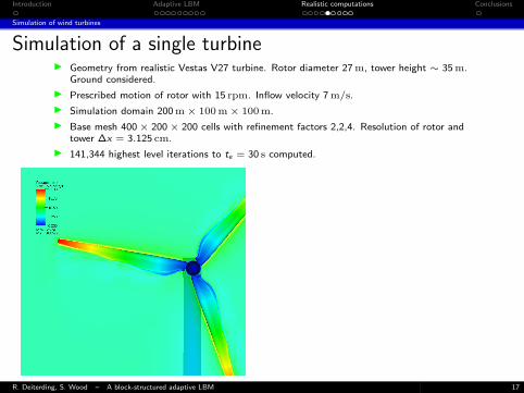
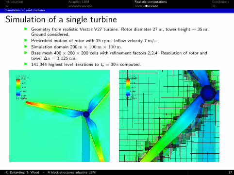
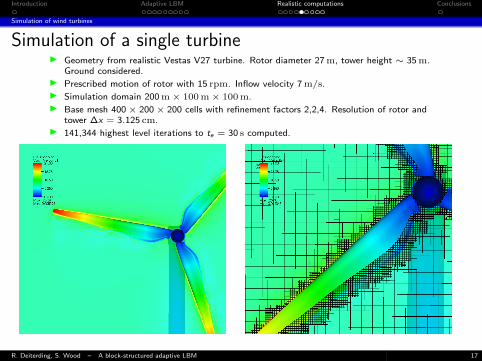
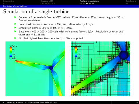
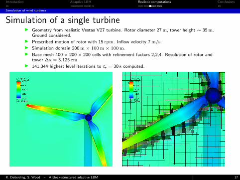
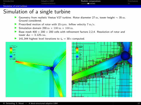
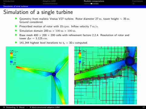
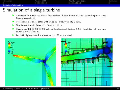
Simulation of a single turbineI Geometry from realistic Vestas V27 turbine. Rotor diameter 27 m, tower height ∼ 35 m.
Ground considered.
I Prescribed motion of rotor with 15 rpm. Inflow velocity 7 m/s.
I Simulation domain 200 m× 100 m× 100 m.
I Base mesh 400× 200× 200 cells with refinement factors 2,2,4. Resolution of rotor andtower ∆x = 3.125 cm.
I 141,344 highest level iterations to te = 30 s computed.
R. Deiterding, S. Wood – A block-structured adaptive LBM 17
Introduction Adaptive LBM Realistic computations Conclusions
Simulation of wind turbines
Simulation of a single turbineI Geometry from realistic Vestas V27 turbine. Rotor diameter 27 m, tower height ∼ 35 m.
Ground considered.I Prescribed motion of rotor with 15 rpm. Inflow velocity 7 m/s.I Simulation domain 200 m× 100 m× 100 m.I Base mesh 400× 200× 200 cells with refinement factors 2,2,4. Resolution of rotor and
tower ∆x = 3.125 cm.I 141,344 highest level iterations to te = 30 s computed.
R. Deiterding, S. Wood – A block-structured adaptive LBM 17
Introduction Adaptive LBM Realistic computations Conclusions
Simulation of wind turbines
Simulation of a single turbineI Geometry from realistic Vestas V27 turbine. Rotor diameter 27 m, tower height ∼ 35 m.
Ground considered.
I Prescribed motion of rotor with 15 rpm. Inflow velocity 7 m/s.
I Simulation domain 200 m× 100 m× 100 m.
I Base mesh 400× 200× 200 cells with refinement factors 2,2,4. Resolution of rotor andtower ∆x = 3.125 cm.
I 141,344 highest level iterations to te = 30 s computed.
R. Deiterding, S. Wood – A block-structured adaptive LBM 17
Introduction Adaptive LBM Realistic computations Conclusions
Simulation of wind turbines
Simulation of a single turbineI Geometry from realistic Vestas V27 turbine. Rotor diameter 27 m, tower height ∼ 35 m.
Ground considered.
I Prescribed motion of rotor with 15 rpm. Inflow velocity 7 m/s.
I Simulation domain 200 m× 100 m× 100 m.
I Base mesh 400× 200× 200 cells with refinement factors 2,2,4. Resolution of rotor andtower ∆x = 3.125 cm.
I 141,344 highest level iterations to te = 30 s computed.
R. Deiterding, S. Wood – A block-structured adaptive LBM 17
Introduction Adaptive LBM Realistic computations Conclusions
Simulation of wind turbines
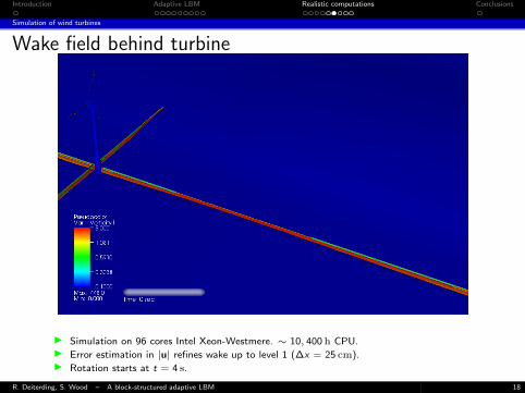
Wake field behind turbine
I Simulation on 96 cores Intel Xeon-Westmere. ∼ 10, 400 h CPU.I Error estimation in |u| refines wake up to level 1 (∆x = 25 cm).I Rotation starts at t = 4 s.
R. Deiterding, S. Wood – A block-structured adaptive LBM 18
Introduction Adaptive LBM Realistic computations Conclusions
Simulation of wind turbines
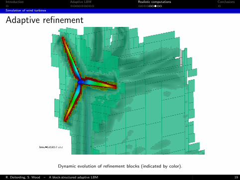
Adaptive refinement
Dynamic evolution of refinement blocks (indicated by color).
R. Deiterding, S. Wood – A block-structured adaptive LBM 19
Introduction Adaptive LBM Realistic computations Conclusions
Simulation of wind turbines
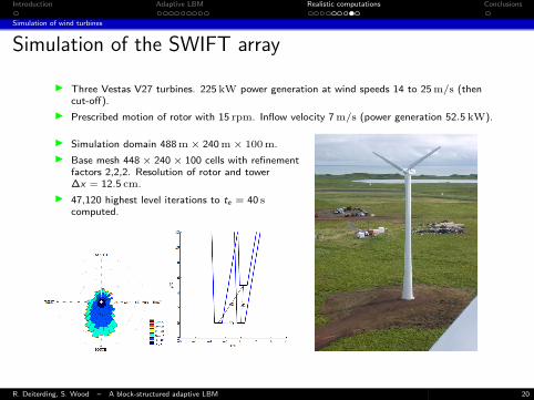
Simulation of the SWIFT array
I Three Vestas V27 turbines. 225 kW power generation at wind speeds 14 to 25 m/s (thencut-off).
I Prescribed motion of rotor with 15 rpm. Inflow velocity 7 m/s (power generation 52.5 kW).
I Simulation domain 488 m× 240 m× 100 m.
I Base mesh 448× 240× 100 cells with refinementfactors 2,2,2. Resolution of rotor and tower∆x = 12.5 cm.
I 47,120 highest level iterations to te = 40 scomputed.
R. Deiterding, S. Wood – A block-structured adaptive LBM 20

Introduction Adaptive LBM Realistic computations Conclusions
Simulation of wind turbines
Wakes in SWIFT array
I Simulation on 288 cores Intel Xeon-Westmere. ∼ 140, 000 h CPU.I Refinement of wake up to level 2 (∆x = 25 cm).I Rotation starts at t = 4 s, full refinement at t = 8 s to avoid refining initial acoustic waves.
R. Deiterding, S. Wood – A block-structured adaptive LBM 21
Introduction Adaptive LBM Realistic computations Conclusions
Things to address
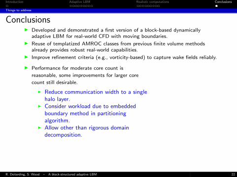
ConclusionsI Developed and demonstrated a first version of a block-based dynamically
adaptive LBM for real-world CFD with moving boundaries.
I Reuse of templatized AMROC classes from previous finite volume methodsalready provides robust real-world capabilities.
I Improve refinement criteria (e.g., vorticity-based) to capture wake fields reliably.
I Performance for moderate core count is
reasonable, some improvements for larger core
count still desirable.
I Reduce communication width to a singlehalo layer.
I Consider workload due to embeddedboundary method in partitioningalgorithm.
I Allow other than rigorous domaindecomposition.
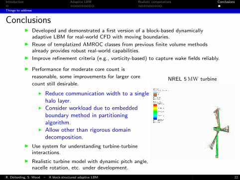
I Use system for understanding turbine-turbineinteractions.
I Realistic turbine model with dynamic pitch angle,nacelle rotation, etc. under development.
NREL 5 MW turbine
R. Deiterding, S. Wood – A block-structured adaptive LBM 22
Introduction Adaptive LBM Realistic computations Conclusions
Things to address
ConclusionsI Developed and demonstrated a first version of a block-based dynamically
adaptive LBM for real-world CFD with moving boundaries.
I Reuse of templatized AMROC classes from previous finite volume methodsalready provides robust real-world capabilities.
I Improve refinement criteria (e.g., vorticity-based) to capture wake fields reliably.
I Performance for moderate core count is
reasonable, some improvements for larger core
count still desirable.
I Reduce communication width to a singlehalo layer.
I Consider workload due to embeddedboundary method in partitioningalgorithm.
I Allow other than rigorous domaindecomposition.
I Use system for understanding turbine-turbineinteractions.
I Realistic turbine model with dynamic pitch angle,nacelle rotation, etc. under development.
NREL 5 MW turbine
R. Deiterding, S. Wood – A block-structured adaptive LBM 22
References
References I
[Berger and Colella, 1988] Berger, M. and Colella, P. (1988). Local adaptive meshrefinement for shock hydrodynamics. J. Comput. Phys., 82:64–84.
[Chen et al., 2006] Chen, H., Filippova, O., Hoch, J., Molvig, K., Shock, R., Teixeira,C., and Zhang, R. (2006). Grid refinement in lattice Boltzmann methods based onvolumetric formulation. Physica A, 362:158–167.
[Deiterding, 2011] Deiterding, R. (2011). Block-structured adaptive mesh refinement- theory, implementation and application. European Series in Applied and IndustrialMathematics: Proceedings, 34:97–150.
[Deiterding et al., 2009] Deiterding, R., Cirak, F., and Mauch, S. P. (2009). Efficientfluid-structure interaction simulation of viscoplastic and fracturing thin-shellssubjected to underwater shock loading. In Hartmann, S., Meister, A., Schafer, M.,and Turek, S., editors, Int. Workshop on Fluid-Structure Interaction. Theory,Numerics and Applications, Herrsching am Ammersee 2008, pages 65–80. kasseluniversity press GmbH.
R. Deiterding, S. Wood – A block-structured adaptive LBM 23
References
References II
[Deiterding et al., 2007] Deiterding, R., Cirak, F., Mauch, S. P., and Meiron, D. I.(2007). A virtual test facility for simulating detonation- and shock-induceddeformation and fracture of thin flexible shells. Int. J. Multiscale ComputationalEngineering, 5(1):47–63.
[Deiterding et al., 2006] Deiterding, R., Radovitzky, R., Mauch, S. P., Noels, L.,Cummings, J. C., and Meiron, D. I. (2006). A virtual test facility for the efficientsimulation of solid materials under high energy shock-wave loading. Engineeringwith Computers, 22(3-4):325–347.
[Deiterding and Wood, 2013] Deiterding, R. and Wood, S. L. (2013). Paralleladaptive fluid-structure interaction simulations of explosions impacting buildingstructures. Computers & Fluids, 88:719–729.
[Hahnel, 2004] Hahnel, D., editor (2004). Molekulare Gasdynamik. Springer.
[Mauch, 2000] Mauch, S. (2000). A fast algorithm for computing the closest pointand distance transform. SIAM J. Scientific Comput.
[Peng and Luo, 2008] Peng, Y. and Luo, L.-S. (2008). A comparative study ofimmersed-boundary and interpolated bounce-back methods in lbe. Prog. Comp.Fluid Dynamics, 8(1-4):156–167.
R. Deiterding, S. Wood – A block-structured adaptive LBM 24


![From Lattice Boltzmann Method to Lattice Boltzmann Flux … · From Lattice Boltzmann Method to Lattice Boltzmann Flux Solver Yan Wang 1, ... flows [8,13–15], compressible flows](https://img.pdfslide.us/doc/110x75/5cadf91b88c9938f4d8c0cd6/from-lattice-boltzmann-method-to-lattice-boltzmann-flux-from-lattice-boltzmann.jpg)


![Improving computational efficiency of lattice Boltzmann ... · 1.1 The lattice Boltzmann method The lattice Boltzmann method [7] [20] is a relative new technique to CFD. Classical](https://img.pdfslide.us/doc/110x75/5f03952b7e708231d409c3df/improving-computational-efficiency-of-lattice-boltzmann-11-the-lattice-boltzmann.jpg)