Supervisor: Stefan Karlsson

Examiner: Mattias Bäckström

E-mail: Isabelle.berg90@gmail.com

Validation of MP-AES at the quantification of trace metals in heavy matrices with comparison of performance to ICP-MS

A bachelor diploma work by Isabelle Berg

P a g e 1 | 31

Abstract: The MP-AES 4200 using microwave plasma and an atomic emission spectroscopy detector provide a new and improved instrument to the analytical field. In this project will the performance of the equipment be evaluated in controlled NaCl-heavy matrices for selected metals (Cu, Zn, Li) and the result from this will be used to optimize a method for specific samples. These samples consist of combustion ashes from the incineration of hazardous waste and are provided by the company SAKAB AB. The sample preparation consisted of several cycles of L/S 10 followed by microwave assisted dissolution with concentrated HNO3, aqua regia or 18.2 MΩ. An extended amount of metals were quantified for these samples (Al, As, Ba, Ca, Cd, Cr, Cu, Fe, K, Li, Mn, Na, Ni, Pb, V, Zn) and most (not Ca, Li, K or Na) were compared with an ICP -MS instrument equipped with a collision cell used for the elements As, Fe and V. A final experiment was made on an L/S 10 of the samples to attempt to separate the metals from the salt with ion exchange, something

that would make it possible to recycle this otherwise unused waste.

The detection limits were all in the low µg L-1 except for Cd, Mn and Zn, which were between 2-4 µg L-1. The MP-AES was found to be able to handle matrices up to 5 g L-1 NaCl without a significant loss of response and provided near identical results to the ICP-MS for the elements that could be compared, this did not included the elements not quantified with the ICP-MS or V which was the only element under the limit of detection for the MP-AES. The experiment where an attempt was made to separate the metals from the salt was

proven successful after treatment of bark compost and another type of waste ash as cation exchangers.

Keywords: MP-AES, ICP-MS, high matrices, digestion, microwave plasma, combustion ash, ion exchange

1 INTRODUCTION

The incineration of biofuels as well as hazardous waste (e.g. oil, solvents, paint [1]) generates ashes which

contain a complex mixture of silicates, oxides, carbonates and residues from not completely combusted

carbon compounds. They also contain a wide range of different metals and has a concentration of salt —

mainly chlorides — that greatly exceeds the 35 ‰ found in seawater. These properties make the leachates

an environmental problem and the ashes must therefore be disposed of under highly controlled conditions,

which is costly for the producers. Since brines are used for several different purposes such as de -icing of

roads there is a chance to re-cycle the leachates provided that the metal content can be kept at

environmentally safe levels. This calls for a robust analytical technology since the matrix will induce

interferences with several common techniques such as AAS and ICP-MS. In this study the performance of the

MP-AES 4200 (Microwave Plasma – Atomic Emission Spectroscopy) will be critically evaluated for the

potential use for metal quantification in brines. The parameters included are the use of internal standards,

matrix matching and ionization suppression as a function of salt concentrations in controlled solutions (NaCl)

as well as leachates. If successful, an instrumental method will be optimized for the use of MP -AES for these

kinds of matrices. The last part of the study evaluates the use of two adsorbents produced from refuse for

the separation of the toxic metals from the brines. Thus, the high salt concentrations play several roles in

this project: Firstly a new analytical technology will be evaluated for this complex matrix and secondly there

will be an effort to remove environmentally toxic metals allowing for re-use of the brines. The ashes used in this work were acquired from the company SAKAB AB located in Sweden.

The high level of salt in the samples causes interferences with several traditional instrumental methods for

metal quantification. In ICP-MS (Inductively Coupled Plasma – Mass Spectrometry) the high chloride

concentration in the matrix needs to be diluted to the low mg L-1 range or exchanged for a less interfering

anion. An alternative is to use an instrument that is equipped with a reaction-/collision-cell. This is due to the

P a g e 2 | 31

poly-atomic interferences that form in the argon plasma when the chloride ions combine with other ions

and/or neutrals. Since the ICP-MS is based on the detection of specific mass/charge ratios the polyatomic

species can increase apparent intensities for elements with the same ratios, or decrease them if the analyte

of interest is combined with chloride. For this type of matrix ICP-OES (Inductively Coupled Plasma – Optical

Emission Spectroscopy) could be an alternative. Since this technique uses optical detection it is less sensitive

to matrix effects from chloride why the polyatomic compounds that are formed has little impact on the

performance and can be compensated for by matrix matched calibration solutions. An even better

performance is expected if the detection is limited to atom lines since the ionic strength will influence the

ionization efficiency. Unfortunately, ICP-OES is more sensitive to elements in groups 1 and 2 because of their

low excitation and ionization energies why it has poorer detection-limits for transition elements compared

to ICP-MS. This makes MP-AES an interesting alternative because of its lower plasma temperature which also

makes controlling the ionization of the matrix easier.

Controlling the ionization of the matrix is desirable since the MP-AES as already mentioned gives a higher

reproducibility when determining atom lines opposed to ion lines, thanks to its relatively cold plasma. The

plasma is however still hot enough to ionize the analytes to a certain extent which will lower the sensitivity if

not dealt with. A reliable method to deal with this type of interferences is to add an ionization inhibitor,

preferably CsNO3, characterized by its low ionization energies which will cause this element to be the first to

form positive ions and thereby inhibit the ionization of the analytes of interest by absorbing excess energy.

Caution must however be taken not to add an excessive amount since this will overload the capacity of the

plasma and thus lower the sensitivity. Evaluations of the most optimal concentration of CsNO 3 has been

made by Karlsson et al. [2] who concluded that the addition of 1.25 g L-1 CsNO3 gave the best response.

Others that have evaluated the improvement of the plasma by adding easily ionizable elements are Balaram

et.al [3] who found that alkali and alkaline earth metals in general gave an improvement of both

vaporization and atomization conditions of the plasma. It is however necessary to choose an element which will not be an analyte of interest.

The hardware for the microwave plasma is somewhat similar to that

of the inductively coupled plasma in that near identical sample

introduction systems, see figure 1, with peristaltic pumps are used

followed by production of an aerosol of the sample with the help of

a nebulizer and selection of its droplet size by spray chamber [4], [5].

Different nebulizer designs can be used although Meinhardt,

MiraMIst and MicroMist are common in both systems. For MP the

recently developed OneNeb has gained increased use because of its

stability and rather high acceptance for particles [6]. The largest

difference between MP AES and ICP-OES is the generation of the plasma. In the traditional Ar plasma used in

ICP it operates around 8000-10 000°C and is generated by energy from electromagnetic radiofrequencies. In

the MP plasma the temperature is roughly half of the Ar ICP, i.e. a temperature around 5000°C. Not only are

the temperatures different, in the MP nitrogen gas is used and the plasma is generated from a magnetic field

that is created by microwaves. This magnetic field is sustained and concentrated with a magnetron and a

waveguide positioned at either side of the torch. The different operating temperatures are of course

dependent on the different ionization potentials of the elements in the plasma gas. Another consequence is

that the Ar ICP plasma has a higher electron activity which means that it has a lower redox potential than the

Figure 1: A picture of a sample introduction starting kit for MP-AES 4200 which can be purchased from: http://www.chem.agilent.com/en-US/products-services/parts-supplies/spectroscopy/mp-aes/mp-aes-sample-introduction-kit-supplies/Pages/default.aspx

P a g e 3 | 31

N2 plasma used in MP. Another important difference for the operator is the running cost. For most ordinary

laboratories argon has to be purchased either in bottles or in the liquid state whereas nitrogen gas for the

MP can easily be extracted from the air with a gas generator [4], [7], [8].

The microwave plasma has been used for nearly three decades although much of the early research is the

result of locally developed laboratory instruments that did not reach a broader market. It was not until 2011

that the instrument became commercially available when Agilent Technologies released the 4100 MP -AES

instrument. Historically a wide range of plasma sources (He, O2, and Ar as well as several combinations

between the former e.g. He + O2 and O2 + Ar) have been evaluated to sustain a stable microwave plasma

[9]–[13]. There has also been less successful attempts to use the air but the current research is focusing on

the use of N2 because of accessibility and economy [2], [14], [15]. The MP has also been coupled to several

different analyzers such as OES, MS, and AES and has been used in a variety of fields with hyphenations like GC-MP-AED [9], [16]–[18].

A downside with an instrument this new is the limited number of publications on its pe rformance for

different applications, i.e. matrices and elements. In fact, since the Agilent MP 4100 was released in 2011

only four articles have reported on the performance of the system, two were published in 2013, one in 2014

and one in early 2015. They concluded, however, that the analytical quality the 4100 MP-AES is comparable

to that of instruments using Ar ICP designs, with the added bonus of a far cheaper analysis [2], [3], [15], [19].

There is also plenty of information from the Agilent Technologies application notes and technical overviews

[20], [21]. Some recent research has also been reviewed in Geostandards and Geoanalytical with the

conclusion that MP-AES is a promising new technique although in need of further research [22]. At the

moment there is no research available that evaluates the performance of the MP-AES when used for semi-trace and trace metal quantification in heavy matrices such as brines, which is the objective of this project.

The final part in this report will attempt to remove metals from the salt-solution from the ash samples by

treatment with solid material capable of exchanging ions. Two complex materials will be examined, both

bark compost and a certain combustion ash. These materials have hypothetically the ability to exchange cat-

ions from the sample solutions and their capacities would be increased if conditioned in an appropriate way.

This treatment aims to generate as many negatively charged sites as possible, i.e. mainly deprotonation of

carboxylic and hydroxyl groups in an attempt to maximize the cation exchange capacity of the materials. The

positively charged metals from the sample solution will thus sorb to the solid material while most of the salt

stay in the solution inducing the desired separation. The properties of the bark compost are fairly well

known since it has been used for metal adsorption in other experiments [23] and this particular batch has

been used in similar experiments (Sjöberg and Karlsson, pers. comm.). The properties of the sludge ash have

not been elucidated in detail so far but from element determination and FTIR spectra it is known that it can

be regarded as a ferric oxide (Karlsson, pers. comm.). This is due to the use of iron as a precipitation agent in the treatment of the sewage water followed by incineration under oxidic conditions in the kiln.

To sum up the objectives this project will deal with; the performance of the MP -AES 4200 in heavy NaCl

matrices and the effect this salt has on the detection limits will be evaluated. This will be followed by the

optimization of a method that can handle this type of matrices while examine the metal content in the ash

samples provided by SAKAB. Finally an attempt will be made to separate the metals from the salt in said samples.

P a g e 4 | 31

2 MATERIALS AND METHODS

2.1 STUDY DESIGN The performance of the MP-AES was evaluated with brines whose properties were either known by

dissolving NaCl or unknown from water extraction of the ashes. The highest tolerable salt concentrations

were determined for the use of i) internal standards, ii) ionization suppression, iii) standard addition and iv)

matrix calibration. Combinations of techniques were also evaluated in order to optimize the analysis with

respect to detection limits, accuracy and time for sample preparation. The separation of metals from salt

was also conducted with the help of material capable of ion exchange. The experimental design and methods will be described in more detail below.

2.2 CHEMICALS AND MATERIALS A mixed calibration solution-stock was prepared from single element solutions by Merck Certipure (Al, As,

Ba, Be, Ca, Cd, Co, Cr, Cu, Fe, K, Li, Mg, Mn, Mo, Na, Ni, Pb, Sr, Zn) and VWR Prolabo (V) to the concentration

10 mg L-1 in 1% HNO3. This stock was diluted for calibration of the MP-AES in the range 0.1-10 mg L-1. It was

also used to prepare controls which were quantified with the samples. The 1% HNO3 used for dilutions

throughout the project was prepared from 18.2 MΩ water and ultrapure HNO 3. The water was produced

with a purification unit and the metal content was evaluated weekly with ICP-MS in a clean-room environment.

Another solution of La, Lu and Y was prepared from single-element solutions (Inorganic Ventures inc.) of

which 100 µL to 10 mL was added to each sample to the concentration of 1.0 mg L-1. These elements

functioned as internal standards. The last stock prepared was with CsNO3-salt (Alfa Aesar, 99.8% pure) to the

concentration of 1.25 g L-1. This was added to each run through the Y-piece via a tygon tubing. For part 1

several concentrations of CsNO3 was evaluated and prepared in the concentration range 0.625-5 g L-1. Both

of the mentioned stocks was diluted using 1% HNO3.

When filtering is mentioned 0.2 µm polypropylene filters were used with syringes unless otherwise specified.

All the tubes used were Sarstedt 15 and 50 mL plastic tubes, glassware was avoided as much as possible but for part one 100 mL glass beakers was used to dry salts in the oven.

2.3 INSTRUMENTAL The settings for the MP-AES and ICP-MS can be found in table 1. In addition to those settings the viewing

position and nebulizer flow for the MP-AES were optimized before each run. Wavelengths and isotopes used

for quantification are shown in table 2. The MP 4200 used for this project was equipped with a concentric

nebulizer and double pass cyclonic spray chamber. Inner diameters of the tube s used was 0.89 mm for

sample introduction and 0.19 mm for the tube used to inject CsNO3 to the sample. Other tubes used was for

spray chamber waste disposal and for transporting rinsing solution. All hardware and tubes were purchased from Agilent except a 0.19 mm tube that was purchased from Idex health and science: Ismatec.

P a g e 5 | 31

Table 1: Instrumental settings for the MP-AES 4200 and ICP-MS used to

evaluate the performance of the MP-AES as well as quantify the metal concentration in ash samples provided by SAKAB AB. MP-AES Argon (L/min) N/A*

Read time (s) 3

Pump speed (rpm) 10

Stabilization time (s) 20 Sample uptake time (s) 45 Rinse time (s) 90

ICP-MS RF power (kW) 1.5 Carrier gas (L/min) 0.9 Makeup gas (L/min) 0.2 Nebulizer pump (rps) 0.1 Replicates 2 Integration time (s) 0.1 Stabilization time (s) 20

*=only used to ignite the plasma

Table 2: Complete wavelenghts and masses analyzed with MP-AES and

ICP-MS respectively to evaluate the performance of MP-AES. MP-AES ICP-MS

Wavelength (nm) Mass

Al 396.152a 27

As 234.984a 75 (ORS)

Ba 455.403i; 553.548a 137

Ca 422.673a - Cd 228.802a 111 Cr 425.433a 53 Cu 324.754a; 327.395a 63 Fe 371.993 56 (ORS) K 766.491a - La (IS) 394.910i; 408.672i Lu (IS) 261.542i; 547.669i Li 610.365a; 670.784a - Mn 403.076a 55 Na 588.995a - Ni 352.454a 60 Pb 368.346a; 405.781a 208 Y (IS) 437.494i; 371.029i V 437.923a 51 (ORS) Zn 213.857a; 481.053a 66

a=atom lines i= ion lines ORS: octopole reaction system

The analytical cycle of the MP-AES thus consisted of 45 seconds sample uptake, 20 seconds to stabilize, then

reading elements at preselected wavelengths and finally rinsing for 90 seconds with 1% HNO3. For ICP-MS

the analytical cycle consisted of 60 seconds rinsing with 18.2 MΩ water following by 60 seconds rinsing with

1% HNO3, 60 seconds sample uptake then 20 seconds to stabilize. The quantification were based on two injections with 0.1 seconds integration time and with peak pattern: full quant.

P a g e 6 | 31

An octopole reaction cell was used with elements sensitive to interferences, see table 2, with the He gas

flow set on 5.0 mL/min. The parameters for the octopole were 180 V for octopole RF and -20.0V for octopole

bias in both normal mode and reaction mode.

2.4 PART 1: MP-AES RELIABILITY AT DIFFERENT NACL-CONCENTRATIONS

2.4.1 Preparation of samples with different concentrations of NaCl

A NaCl-solution was prepared by dissolving the salt in 1% HNO3 with consideration taken to the purity

(98.8%). A stock solution was prepared from Cu(NO3)2, ZnSO4 and a 1.0 mmol/L standard solution (Li)

respectively in 1% HNO3. Before preparation the salts were dried at 105ᵒC. Li was diluted from 1 mmol/L to 1 mg L-1. This stock-solution was diluted 20 times to get within the calibration range of Cu and Zn.

From the diluted metal-stock 1.5 mL was transferred to 15 mL test tubes (Sarstedt) and then the NaCl-

solution (100 g L-1) was added to give concentrations in the range 0-50 g L-1. Finally the volume was adjusted

to 15 mL with 1% HNO3. A sample with 100 g L-1 NaCl was prepared by dissolving NaCl directly in the test

tube. Another set of samples containing only the NaCl were also prepared in the range 0-50 g L-1 to

determine if there were any interferences present in the NaCl. Internal standard was added manually to

each sample.

The samples for evaluation of the detection limits were prepared by adding 3 mL of 1% HNO3 in 15 separate

tubes, this series of blanks was compared to a set of 15 samples containing 5 g L-1 NaCl in 1% HNO3. Both series also contained internal standards.

2.4.2 Experimental design for part 1

The samples were used to study if ionization suppression was enough to provide reliable results. They were

therefore quantified without further preparation in a series of CsNO3-concentrations that ranged from 0.625

to 5 g L-1 to determine the optimal conditions for this kind of matrix. All instrument signals were interpreted

by the MP Expert software. The samples for detection limit evaluation were quantified only in the presence

of 1.25 g L-1 CsNO3.

2.5 PART 2: METHOD OPTIMIZATION FOR QUANTIFICATION OF METALS IN COMBUSTION ASHES

2.5.1 Preparation of combustion ash – samples

Multiple samples were prepared to better determine the precision of the experiment. Knowing that the

samples contained a high amount of salt that could interfere with the quantification they were first leached

with 18.2 MΩ water. This was done by weighing up three replicate samples of 4 g each adding 40 mL 18.2

MΩ water to reach an L/S of 10, shaking them for 30 minutes and then centrifuge them at 5000 rpm for 20

minutes. The solution phase was measured for electrical conductivity as a proxy for ion concentrations. Finally, the L/S 10 leaching was repeated until the electrical conductivity reached a constant value.

After the leaching was completed the solid samples were dried overnight at 40ᵒC, crushed with a mortar and

pestle to finer particles, and then dried during the day at 55ᵒC until constant weight. From the dry samples

0.1 g was transferred to three separate Teflon tubes used in a CEM MarsV microwave digestion system. To

these samples either 10 ml of concentrated HNO3, Aqua Regia or MΩ were added, respectively. Three blanks

with only the acids or 18.2 MΩ water was added. The samples were then digested in two steps: the first

reached a maximum temperature of 180ᵒC after 30 minutes at 300 W exposure; the second remained at this

temperature for another 30 minutes with a power of 600 W. The samples were then allowed to cool for an

additional 30 minutes before getting transferred to 50 mL test tubes (Sarstedt) and adjusted to the volume

P a g e 7 | 31

of 50 mL. This was made with 18.2 MΩ water for the samples digested with HNO 3 and aqua regia or 1% HNO3 for the samples digested with 18.2 MΩ water only.

The samples were then filtered to remove residues like solid silicates which the chosen digestion procedure

does not dissolve. To solubilize silica HF is required but due to the highly hazardous nature of this acid it was

omitted from the sample preparation. This is also motivated by the fact that only minute amounts of the

elements studied are entrapped in silicate structures that are formed either during incineration or acid

treatment. The filters were rinsed with 1% HNO3 which was saved for quantification and the filtered samples

were diluted with 1% HNO3 to suit the calibration range. For MP-AES dilutions of 10 and 100 times were

used while the lower detection limits of ICP-MS required dilutions of 100 and 1000 times. Two controls of

0.1 and 1 mg L-1 were prepared from the 10 mg L-1 multi-elemental stock. Lastly internal standards (La, Lu and Y) were added manually to each MP-AES sample and Rh to the ICP-samples.

To examine the interferences a standard addition was made by mixing selected samples in the proportion 1:1 with the blank, 0.5 mg L-1 standard and 1 mg L-1 standard respectively.

2.5.2 Experimental design for quantification of metals in combustion ashes

The dried ash samples were examined with FTIR to determine the possible remains of organic material. This

was especially made to determine if there still was any soot left that could be difficult to dissolve with the

chosen method.

All MP-AES quantifications in this part of the project were done with the CsNO3-concentration that gave the

best response in part 1 of the project. The CsNO3 were automatically added through the Y-piece for the MP-

AES 4200. After the filtrated digests had been diluted with 1% HNO3 internal standards were added. The

samples were quantified in the MP-AES with optimized settings to determine the concentration of certain

metals and in ICP-MS for comparison. Additional quantifications were performed on the filtrate water from digests using the same settings as above to see if any metals was lost in this step.

To complete the evaluation of method accuracy a series of matrix adjusted calibration solutions and

standard addition using both calibrations were investigated. This allows for a direct comparison with the

original standard addition procedure to determine if a matrix adjusted calibration could enhance the

accuracy in these heavy matrices. These standards were prepared in the same way as described under

section 2.1 chemicals and with the additions from a NaCl stock solution to give a final concentration of 2 mg L-1.

2.6 PART 3: REMOVAL OF HEAVY METALS FROM BRINES

2.6.1 Preparation of samples for the separation of metals and salt

A new stock solution of metals was prepared for this experiment from 9 single-element solutions (Ni, Cr, Fe,

V, Zn, Cd, Cu, Mn, Pb) and 1 salt (LiCl). The solutions were prepared in 1% HNO 3 to give a final concentration

of 100 mg L-1 of each element. Four new ash samples were leached with 18.2 MΩ water in the same way as

in section 2.4.1 to give a matrix suitable for separation of metals and salt. After the centrifugation and

filtration of these brines 9 mL of was transferred to two 15 mL test tubes and to these 1 mL of the metal-

stock was added, thus increasing the metal concentration of the samples with 10 mg L-1. This was done to

ensure that the chosen metals would be present for the separation. For comparison were two samples

prepared from the brines with no stock added and two samples were prepared with a controlled matrix. The latter contained a known concentration of NaCl and 10 mg L-1 added metals from the stock.

Pretreatment of the solid material that was to be added as ion exchange material consisted of the following.

The bark compost was allowed to hydrate in deionized water for roughly 2 hours and then filtered through a

P a g e 8 | 31

2.5 µm cellulose acetate filter using a Büchner funnel and vacuum flask to get rid of excess water. The

pretreatment of the dry sludge ash consisted only of milling that was followed by sieving (1 mm). Before

adding these adsorbents the pH of the sample solutions was adjusted to 10-11 for the bark compost systems

since it is within the range of the L/S 10 value for leachates of fresh incineration ashes. For the systems with

sludge ash the pH was set to 8.0-8.5 because of the increased solubility of ferric oxides at high pH because of

the formation of negatively charged hydroxides. When the systems had been prepared in 50 ml test tubes they were put on an end-over-end rotary tumbler and allowed to equilibrate overnight.

2.6.2 Experimental design for part 3: removal of heavy metals

Prior to the metal quantification the samples were centrifuged for 10 minutes at 5000 rpm, filtered through

0.2 µm syringe filters and diluted 10 and 100 or 100 and 1000 times with 1% HNO3. Samples taken before

the addition of adsorbents were diluted more since they were expected to contain more metals. Internal

standards were added to all samples and they were quantified with 1.25 g L-1 CsNO3 added through the Y-

piece. The quantification was made together with two controls of 0.1 and 1 mg L-1. The controls were

prepared from the 10 mg L-1 multi-elemental stock described in section 2.1 by diluting the stock with 1% HNO3 and adding internal standards.

2.7 QC/QA Several steps were taken to improve the quality control and assurance such as the use of a method blank

going through all of the steps with the real samples in part 2 and the samples with a controlled matrix in part

3. The use of multi-elemental controls were added with most of the MP-AES analysis to evaluate the

machines performance and to further improve the instrumental progress also internal standards and

replicates were used for both instruments. Multiple samples were also prepared in each experiment to minimize human error.

When it came to equipment and chemicals glassware were avoided as much as possible to avoid the

adsorption of metals that occurs in glassware and the samples was only kept in polypropylene-tubes. Care

was taken that the chemicals and other equipment were sufficiently clean. Finally, statistics such as relative standard deviation and confidence intervals was performed were applicable on the results.

3 RESULTS AND DISCUSSION

3.1 PART 1: EVALUATION OF MP-AES PERFORMANCE IN HIGH MATRICES To correct for background interferences for MP-AES in this project the auto background correction mode in

the MP Expert software was used unless an interference was present when off-peak right/left was used. The

interferences that could be corrected for by this function were unless otherwise specified Pb 368.346, Zn

213.857, Fe 371.993 and Cr 425.433 where in all cases off peak right were used.

3.1.1 Evaluation of the impact salt had on the intensities of chosen wavelengths

The calibration error given by the MP-AES Expert Software was 5% and the linear regression were 1.0 for all

elements since only a 1-point calibration was used with a 5 mg L-1 standard. This was due to the qualitative nature of this part of the project with a main focus on the intensities.

The evaluated elements and their atom lines (nm) were: Cu 324.754, Cu 327.395, Zn 213.857, Zn 482.053, Li

610.365 and Li 670.784. Of these copper 324.754 and zinc 213.857 had signal intensities at 450’000 and

580’000 c/s respectively in the 5 mg L-1 standard and in the presence of 1.25 g L-1 CsNO3. This can be

compared with the 327.395 and 482.053 nm lines which gave intensities of 240’000 and 1750 c/s. For lithium

P a g e 9 | 31

the intensities were 4’000’000 c/s on the 670.784 nm compared to 40’000 c/s on the 610.365 nm. The latter

wavelength was not able to give a response when quantifying the samples. The wavelengths chosen for

analysis were the ones giving the highest intensity.

Figure 2-4 represent the results of the quantifications as a function of the concentration of NaCl. For copper

324.754 and zinc 213.857 the drop in intensity is steep and inversely exponential after amounts higher than

1 g L-1 NaCl is present in the solution phase, see figure 2 and 3. The by far largest drop in intensity occurs

after addition of 25 g L-1 NaCl. Up to 1 g L-1 NaCl the drop was marginally for zinc. In the presence of 1.25 g L-1

CsNO3 it declined from 27’000 to 24’000 c/s while after adding 25 g L-1 it declined to 14’000 c/s from the

38’000 c/s at 12.5 g L-1 NaCl. Copper is showing a similar pattern although it increases marginally up to the

concentration of 1 g L-1 NaCl. The increase is from 620’000 c/s when no NaCl is added to 660’000 c/s at 1 g L-1

NaCl. After 1 g L-1 NaCl the same steep reduction in intensity is however shown from the 660’000 c/s at 1 g L-

1 it decreases to 45’000 c/s at the highest concentration of 100 g L-1 NaCl.

The previous data are from the quantification performed with the addition of 1.25 g L-1 CsNO3 through the Y-

piece to the sample. Similar patterns are however seen for all concentrations of added CsNO3 although

copper at most concentrations of CsNO3 (0-1.5 g L-1) had the highest intensity at 0.5 g L-1 added NaCl. This

also was true in some cases for zinc (0.625, 1 and 2.5 g L-1 CsNO3). The same pattern as for 1.25 g L-1 CsNO3

for copper was shown at the added concentration of 2.5 g L-1 and for zinc at the concentrations of 0 and 1.5

g L-1 CsNO3. Zinc had the highest intensity at 1 g L-1 NaCl and in the presence of 5 g L-1 CsNO3. The highest

intensities at the intermediate concentration of NaCl indicates that copper and zink were undetected due to

ionization in the absence of NaCl. This phenomena will be more thoroughly discussed below but it is a clear

indication that sodium in small quantities can improve the performance of the MP-AES, although too high concentrations will give the opposite result.

For lithium a completely different relationship with the concentration of NaCl was found, see figure 4. For

most concentrations of added CsNO3 the intensity increased instead of decreasing with a higher

concentration of NaCl. For the quantification with 1.25 g L-1 added CsNO3 the intensity increase in a

consistent manner from 6000 c/s at 0 g L-1 NaCl to 24’000 c/s at 100 g L-1 NaCl except for a drop in intensity

between 25 and 50 g L-1 NaCl from 18’000 c/s to 16’000 c/s. All other systems except for the one with 1 g L-1

added CsNO3 showed the same relationship with a steady increase with one or two smaller dips These dips

were around the concentration of 1 g L-1 for most and 5 g L-1 NaCl at the run with 2.5 g L-1 CsNO3. The

quantification with 1 g L-1 added CsNO3 showed however that an optimal condition was achieved between 50

and 75 g L-1 NaCl with lower intensities on both sides in a shape similar to that of a Gaussian curve. A

hypothesis is that the other concentrations of CsNO3 would show a similar relationship if the concentrations of NaCl was high enough.

A possible explanation for the different manner in which lithium respond to increasing level of NaCl can be

related to its ionization energies. Sodium and lithium have similar ionization energies, 495.8 kJ/mole and

520.2 kJ/mole respectively. This can be compared with the ones for copper and zinc at 745.5 and 906.4

kJ/mole or the ionization energy for cesium at 375.7 kJ/mole. As mentioned in the introduction cesium is

added to control the matrix by absorbing excess energy in the plasma and improve the quantification of

other elements by minimizing their ionization. Sodium should give a similar relation since it i onizes at lower

energies than copper and zinc but at higher concentrations of sodium will an increasing part of the plasma

energy be used to excite and ionize sodium and there will therefore not be enough energy left to

quantitatively excite copper and zink. Hence, we get an intensity decrease with increased concentrations of NaCl for these elements.

P a g e 10 | 31

Figure 2: The intensity, in counts per seconds, is given as a function of the concentration of NaCl for Zn 213.857. The different series represent different analyses on the same

samples with an increasing concentration of the ionization-inhibitor CsNO3.

Figure 3: The intensity, in counts per seconds, is given as a function of the concentration of NaCl in for Cu 324.754. The different series represent different analyses on the same

samples with an increasing concentration of the ionization-inhibitor CsNO3.

Figure 4: The intensity, in counts per seconds, is given as a function of the concentration of NaCl for Li 670.784. The different series represent different analyses on the same samples with an increasing concentration of the ionization-inhibitor CsNO3.

Figure 5: The intensity, in counts per seconds, is given as a function of the concentration of the ionization inhibitor CsNO3. The different series represent samples with an increasing

concentration of NaCl, all data is for Cu 324.754.

P a g e 11 | 31

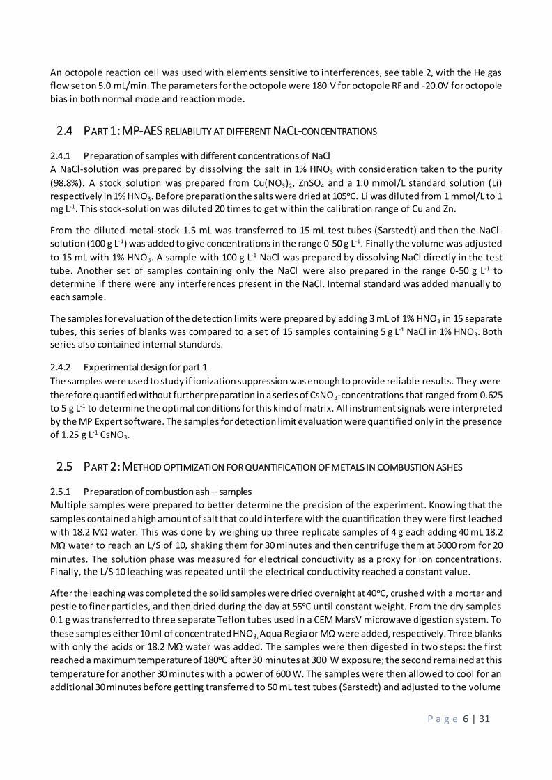
Figure 6: The intensity, in counts per seconds, is given as a function of the concentration of the ionization inhibitor CsNO3. The different series represent samples with an increasing concentration of NaCl, all data is for Cu 324.754.

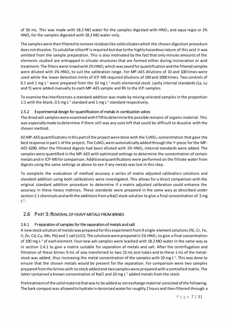
Figure 7: The intensity, in counts per seconds, is given as a function of the concentration of the ionization inhibitor CsNO3. The different series represent samples with an increasing concentration of NaCl, all data is for Li 670.784.

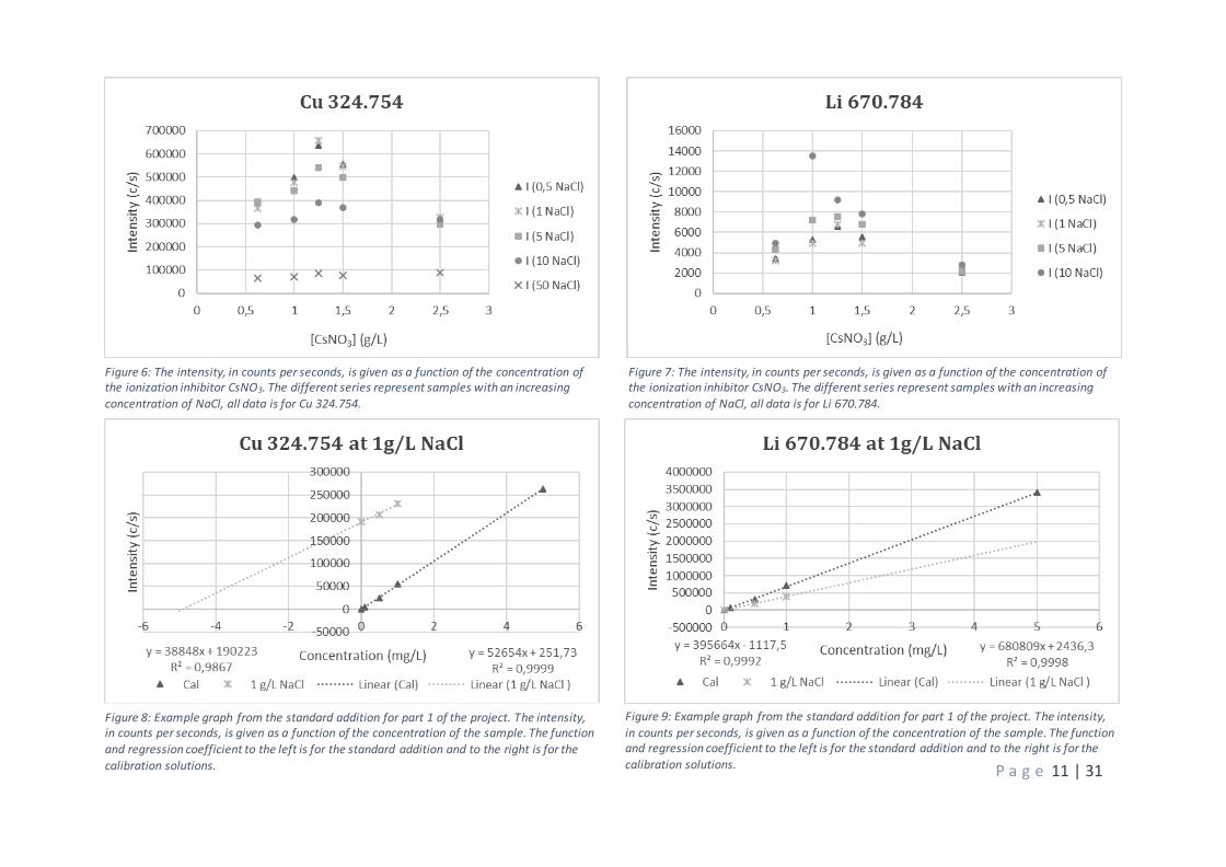
Figure 8: Example graph from the standard addition for part 1 of the project. The intensity, in counts per seconds, is given as a function of the concentration of the sample. The function

and regression coefficient to the left is for the standard addition and to the right is for the

calibration solutions.

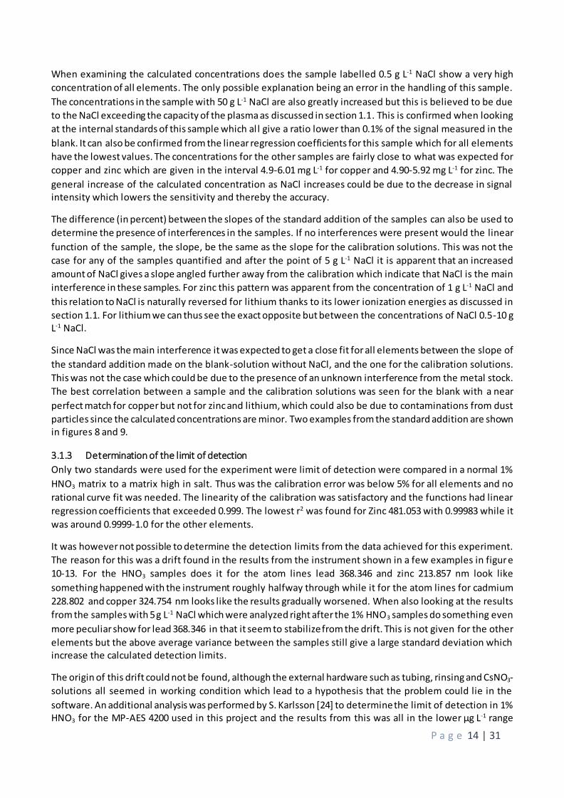
Figure 9: Example graph from the standard addition for part 1 of the project. The intensity,

in counts per seconds, is given as a function of the concentration of the sample. The function and regression coefficient to the left is for the standard addition and to the right is for the

calibration solutions.

P a g e 12 | 31

Lithium however having a much lower ionization energy and being a much smaller atom compared to copper

and zinc will generate an increased signal intensity with increasing concentrations of sodium. This is due to

the lower first ionization energy for lithium. Upon ionization the element is not detected using its atom line.

Upon addition of sodium however a fraction of this element will ionize which lowers the available energy in

the plasma. These conditions lower ionization of lithium and a larger fraction of excited species will form

that increases the signal from the atom line. Because of the similar ionization energies for Li and Na it is

highly likely that the drop seen for the atom line signals for Cu and Zn that was due to the plasma being

overloaded. These conditions are not expected for lithium because of its low atomization energy. Instead we

get the same response for most elements when cesium is added i.e. an increased concentration will increase the signal from an atom line for elements until the capacity of the plasma is exceeded.

Data from the quantification above is also shown in figure 5-7 where the intensity is plotted as a function of

the concentration of added CsNO3 instead of NaCl. This evaluation was done to determine the concentration

of added ionization suppressor that would give the best control of the matrix influenced ionization. As can

be seen in the figures there is a maximum intensity response for the 1.25 g L-1 CsNO3 for all elements in the

study. These results correspond well with the evaluation of plant digests where the optimum concentration

of CsNO3 was found at this concentration [2]. This is not too surprising since high levels of sodium and

potassium are typical for that kind of matrix. Further, from the graphs it can be seen that up to 5 g L-1 of NaCl

sufficiently high intensities from atom lines are present for quantification while the signal depression is very

high at 50 g L-1. Hence, matrices containing 10 g L-1 NaCl would work but higher concentrations require

dilution.

These results confirms the discussion above that addition of the easily ionizable cesium consumes enough

energy from the plasma to allow for the use of atom lines for the other elements. It is, however, very

important to remember that this is applicable only to atom lines, i.e. the emission from the relaxation of

excited atoms. We can also see that the results are similar for Li as well as for Cu and Zn. Hence, the non-

suppressed energy in the plasma is high enough to ionize small and variable fractions of both copper and

zinc. It is therefore recommended to use CsNO3 as ionization suppressor even in a matrix that is dominated

by quite high concentrations of NaCl. When following these guidelines it is also important to monitor the total energy status of the plasma in order to avoid that the plasma is overloaded.

There are also a clear correlation between the intensity of the internal standard elements (La, Lu, Y) and the

concentration of NaCl which is seen as further proof that the capacity of the plasma is exceeded. For

lanthanum 394.910 in the presence of 1.25 g L-1 CsNO3 the signal intensity decreases from 23’000 c/s in the

solution without NaCl addition to some 100 c/s in the sample with 100 g L-1 NaCl. The same can be seen for

all internal standards, some wavelengths (Lu 261.542 and Lu 547.669) are even so low that only an “error”

was given by the software. These results indicate that special care must be taken when quantifying salt-rich

matrices to optimize a method that will not exceed the capacity of the plasma. From this point of view it is

beneficial to include one or several ion lines from the IS elements since loss of signal is a good indicator of

plasma overload. Hence, for each kind of matrix a compromise has to be made concerning the concentration

of the ion suppressor and the need for dilution of the matrix in order to ascertain enough energy for analyte

excitation with a minimum risk for plasma overload. Within reasonable limits this can be accomplished by

optimizing the diameter of the tubing in the ionization suppressor line.

3.1.2 Standard addition for part 1 For this experiment the instrument was calibrated up to the concentration of 10 mg L-1 except for Li 670.784

which only was calibrated up to the concentration 5 mg L-1 because of saturation of the detector. The

quantification of the experiment was divided into two parts: the first containing standard addition of the

samples up to the concentration of 10 mg L-1 and the second concentrations of 50 mg L-1 and control

P a g e 13 | 31

solutions. These will henceforth be called run 1 and run 2. The calibration errors in both runs were fairly low

and for most elements around 10% (Cu 324.754, Cu 327.395 and Li 610.365). Lithium 670.784 and zinc

213.857 were lower in run 1 with both needing a calibration error of 8% while zinc needed a higher

calibration error in run 2 with 11%. Zinc 481.053 were the only element needing a 15% calibration error in

both runs. The linear regression of the calibration fit, r2, were at least 0.999 for all atom lines examined in

this experiment with the lowest value for copper 327.395 in run 1 with 0.99918 and the highest for lithium 670.784 with 0.99999 in the second run.

Evaluation of the intensities gave similar results to the previous experiment. In the 5 mg L-1 calibration

standard the lines for copper 324.754 and 327.395 gave intensities at 260’000 c/s and 130’000 c/s

respectively while the wavelengths for zinc had 1000 c/s at 481.053 nm and 40’000 c/s at 213.857 nm.

Lithium had 33’000 c/s for the 610.365 nm wavelength and 34’000’000 c/s at the 670.784 nm. The former

wavelength for lithium could in this experiment give results for all samples except the ones mixed with the

blank while the latter wavelength gave a results for all samples and thus was chosen for quantification. For copper and zinc the wavelength with the highest intensities were chosen.

The lowered intensities for both determined metals and internal standard elements when the concentration

of NaCl increased were obvious in this part of the project as well. In the first run a decrease is apparent

when comparing the sample with 0 g L-1 NaCl mixed 1:1 with the blank solution and the sample with 10 g L-1

NaCl mixed 1:1 with the same blank. The former has an intensity of 52’000 c/s for yttrium 371.029 nm that is

lowered to 32’000 c/s in the latter. This is lowered even further in run 2 where it for the sample originally

containing 50 g L-1 NaCl now mixed 1:1 with blank is down to 3000 c/s. These data given in ratio related to

the blank is 1.02, 0.64 and 0.05 respectively. Similar results are observed for all internal standards.

Results from the standard addition are shown in table 3. The samples are labelled after concentration of

NaCl in g L-1. All samples have the same concentration of metals added as stated in the method which after

dilution were 5 mg L-1 of copper and zinc and 5 µg L-1 for lithium. The samples labelled blanks do not contain

any added metals only NaCl to examine if the salt added to the metal concentration.

Table 3: Standard addition results for part 1. The concentrations are calculated from the equations given by the

standard addition. The concentration given for NaCl is in g L-1 in the original samples. A value is given for the difference in percentage between the slopes of the sample and the slope represented by the calibration curve, the value of the calibration slope is also given. This run was divided in two Cu 324.754 Zn 213.857 Li 670.784

NaCl g L-1

[Cu] mg L-1

% diff. slope

r2 [Zn] mg L-1

% diff. slope

r2 [Li]

µg L-1 % diff. slope

r2

0 6,01 -41,11 0,809 5,27 -35,61 0,9593 2,71 -42,56 0,994 0.5 14,65 -73,81 0,9955 8,93 -59,65 0,8586 9,52 -46,02 0,9998 1 4,90 -26,22 0,9867 4,90 -30,62 0,9844 2,82 -41,88 0,9992 5 5,09 -25,08 1 5,57 -41,59 0,9998 6,41 -36,65 1 10 5,61 -38,98 0,9996 5,92 -54,73 0,9923 5,61 -35,97 0,9977 50 12,38 -93,07 0,7404 2,53 -90,93 0,6229 30,55 46,88 0,9816 Blank 0 0,00 -2,29 0,9999 0,02 -41,47 0,9981 0,48 -21,35 1

Blank 5 0,13 -13,93 0,8921 0,05 -52,70 1 5,22 -23,02 0,9996

[Cu] mg L-1

slope r2 [Zn] mg L-1

slope r2 [Li] µg L-1

slope r2

Control 0.1 0,1 52654 0,9999 0,09 8007,9 0,9997 0,09 680809 0,9998

Control 1 1,02 1,12 0,99

Control 0,1 0,11 97833 1,0000 0,08 10279,0 0,9997 0,09 1000000* 1,0000

Control 1 0,96 0,99 0,94

* This result was given as 1E+06 in excel.

P a g e 14 | 31

When examining the calculated concentrations does the sample labelled 0.5 g L-1 NaCl show a very high

concentration of all elements. The only possible explanation being an error in the handling of this sample.

The concentrations in the sample with 50 g L-1 NaCl are also greatly increased but this is believed to be due

to the NaCl exceeding the capacity of the plasma as discussed in section 1.1. This is confirmed when looking

at the internal standards of this sample which al l give a ratio lower than 0.1% of the signal measured in the

blank. It can also be confirmed from the linear regression coefficients for this sample which for all elements

have the lowest values. The concentrations for the other samples are fairly close to what was expected for

copper and zinc which are given in the interval 4.9-6.01 mg L-1 for copper and 4.90-5.92 mg L-1 for zinc. The

general increase of the calculated concentration as NaCl increases could be due to the decrease in signal intensity which lowers the sensitivity and thereby the accuracy.

The difference (in percent) between the slopes of the standard addition of the samples can also be used to

determine the presence of interferences in the samples. If no interferences were present would the linear

function of the sample, the slope, be the same as the slope for the calibration solutions. This was not the

case for any of the samples quantified and after the point of 5 g L-1 NaCl it is apparent that an increased

amount of NaCl gives a slope angled further away from the calibration which indicate that NaCl is the main

interference in these samples. For zinc this pattern was apparent from the concentration of 1 g L-1 NaCl and

this relation to NaCl is naturally reversed for lithium thanks to its lower ionization energies as discussed in

section 1.1. For lithium we can thus see the exact opposite but between the concentrations of NaCl 0.5-10 g L-1 NaCl.

Since NaCl was the main interference it was expected to get a close fit for all elements between the slope of

the standard addition made on the blank-solution without NaCl, and the one for the calibration solutions.

This was not the case which could be due to the presence of an unknown interference from the metal stock.

The best correlation between a sample and the calibration solutions was seen for the blank with a near

perfect match for copper but not for zinc and lithium, which could also be due to contaminations from dust

particles since the calculated concentrations are minor. Two examples from the standard addition are shown in figures 8 and 9.

3.1.3 Determination of the limit of detection

Only two standards were used for the experiment were limit of detection were compared in a normal 1%

HNO3 matrix to a matrix high in salt. Thus was the calibration error was below 5% for all elements and no

rational curve fit was needed. The linearity of the calibration was satisfactory and the functions had linear

regression coefficients that exceeded 0.999. The lowest r2 was found for Zinc 481.053 with 0.99983 while it

was around 0.9999-1.0 for the other elements.

It was however not possible to determine the detection limits from the data achieved for this experiment.

The reason for this was a drift found in the results from the instrument shown in a few examples in figure

10-13. For the HNO3 samples does it for the atom lines lead 368.346 and zinc 213.857 nm look like

something happened with the instrument roughly halfway through while it for the atom lines for cadmium

228.802 and copper 324.754 nm looks like the results gradually worsened. When also looking at the results

from the samples with 5 g L-1 NaCl which were analyzed right after the 1% HNO3 samples do something even

more peculiar show for lead 368.346 in that it seem to stabilize from the drift. This is not given for the other

elements but the above average variance between the samples still give a large standard deviation which increase the calculated detection limits.

The origin of this drift could not be found, although the external hardware such as tubing, rinsing and CsNO3-

solutions all seemed in working condition which lead to a hypothesis that the problem could lie in the

software. An additional analysis was performed by S. Karlsson [24] to determine the limit of detection in 1% HNO3 for the MP-AES 4200 used in this project and the results from this was all in the lower µg L-1 range

P a g e 15 | 31

Figure 10: The intensity in counts per seconds shown for all three replicates of 15 samples. The samples with 1% HNO3 is represented on the primary y-axis while the samples with 5 g L-1 NaCl is represented on the secondary axis.

Figure 11: The intensity in counts per seconds shown for all three replicates of 15 samples. The samples with 1% HNO3 is represented on the primary y-axis while the samples with 5 g L-1 NaCl is represented on the secondary axis.

Figure 12: The intensity in counts per seconds shown for all three replicates of 15 samples. Figure 13: The intensity in counts per seconds shown for all three replicates of 15 samples.

The samples with 1% HNO3 is represented on the primary y-axis while the samples with 5 g L-1 NaCl is represented on the secondary axis.

P a g e 16 | 31

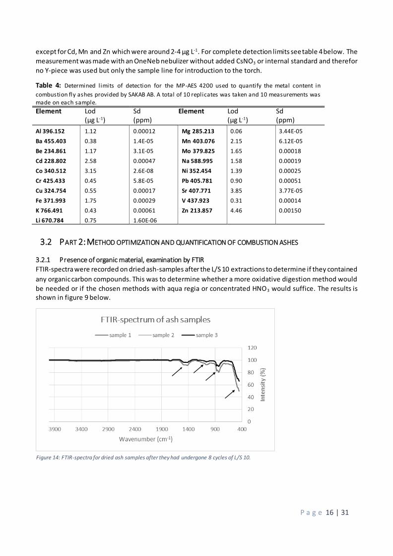
except for Cd, Mn and Zn which were around 2-4 µg L-1. For complete detection limits see table 4 below. The

measurement was made with an OneNeb nebulizer without added CsNO3 or internal standard and therefor

no Y-piece was used but only the sample line for introduction to the torch.

Table 4: Determined limits of detection for the MP-AES 4200 used to quantify the metal content in

combustion fly ashes provided by SAKAB AB. A total of 10 replicates was taken and 10 measurements was made on each sample. Element Lod

(µg L-1) Sd (ppm)

Element Lod (µg L-1)

Sd (ppm)

Al 396.152 1.12 0.00012 Mg 285.213 0.06 3.44E-05

Ba 455.403 0.38 1.4E-05 Mn 403.076 2.15 6.12E-05

Be 234.861 1.17 3.1E-05 Mo 379.825 1.65 0.00018

Cd 228.802 2.58 0.00047 Na 588.995 1.58 0.00019

Co 340.512 3.15 2.6E-08 Ni 352.454 1.39 0.00025

Cr 425.433 0.45 5.8E-05 Pb 405.781 0.90 0.00051

Cu 324.754 0.55 0.00017 Sr 407.771 3.85 3.77E-05

Fe 371.993 1.75 0.00029 V 437.923 0.31 0.00014

K 766.491 0.43 0.00061 Zn 213.857 4.46 0.00150

Li 670.784 0.75 1.60E-06

3.2 PART 2: METHOD OPTIMIZATION AND QUANTIFICATION OF COMBUSTION ASHES

3.2.1 Presence of organic material, examination by FTIR

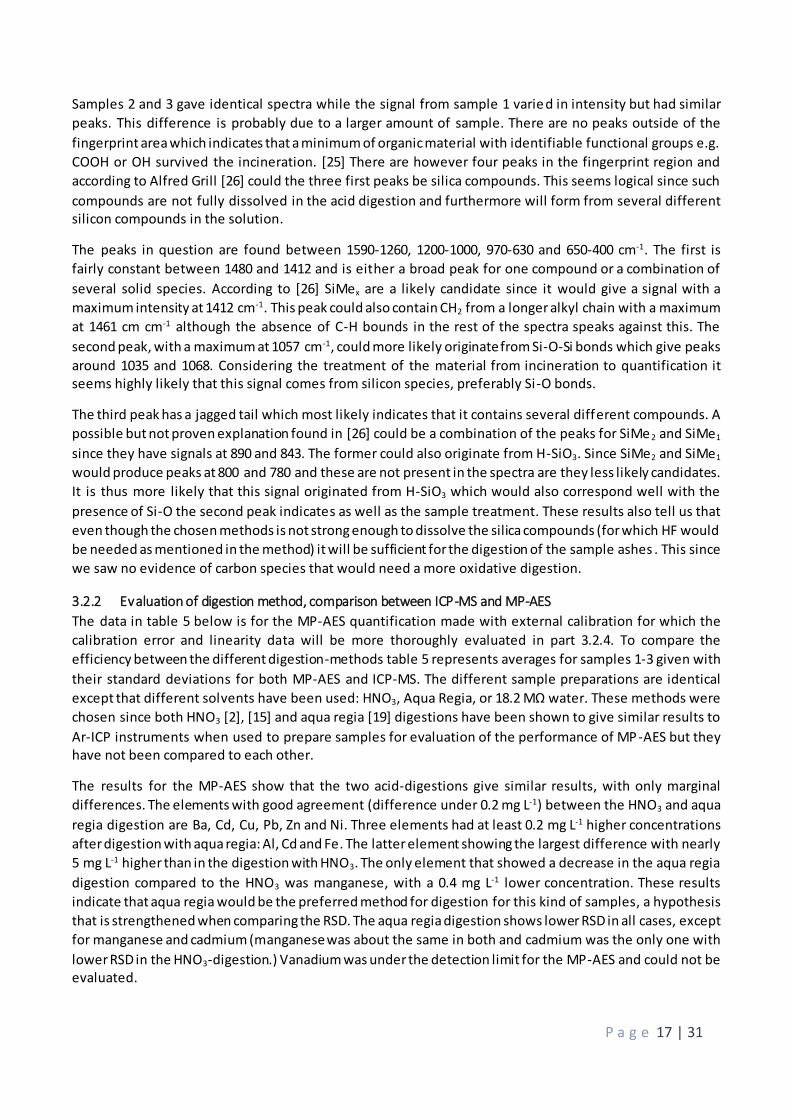
FTIR-spectra were recorded on dried ash-samples after the L/S 10 extractions to determine if they contained

any organic carbon compounds. This was to determine whether a more oxidative digestion method would

be needed or if the chosen methods with aqua regia or concentrated HNO3 would suffice. The results is shown in figure 9 below.

Figure 14: FTIR-spectra for dried ash samples after they had undergone 8 cycles of L/S 10.

P a g e 17 | 31

Samples 2 and 3 gave identical spectra while the signal from sample 1 varied in intensity but had similar

peaks. This difference is probably due to a larger amount of sample. There are no peaks outside of the

fingerprint area which indicates that a minimum of organic material with identifiable functional groups e.g.

COOH or OH survived the incineration. [25] There are however four peaks in the fingerprint region and

according to Alfred Grill [26] could the three first peaks be silica compounds. This seems logical since such

compounds are not fully dissolved in the acid digestion and furthermore will form from several different silicon compounds in the solution.

The peaks in question are found between 1590-1260, 1200-1000, 970-630 and 650-400 cm-1. The first is

fairly constant between 1480 and 1412 and is either a broad peak for one compound or a combination of

several solid species. According to [26] SiMex are a likely candidate since it would give a signal with a

maximum intensity at 1412 cm-1. This peak could also contain CH2 from a longer alkyl chain with a maximum

at 1461 cm cm-1 although the absence of C-H bounds in the rest of the spectra speaks against this. The

second peak, with a maximum at 1057 cm-1, could more likely originate from Si-O-Si bonds which give peaks

around 1035 and 1068. Considering the treatment of the material from incineration to quantification it seems highly likely that this signal comes from silicon species, preferably Si-O bonds.

The third peak has a jagged tail which most likely indicates that it contains several different compounds. A

possible but not proven explanation found in [26] could be a combination of the peaks for SiMe2 and SiMe1

since they have signals at 890 and 843. The former could also originate from H-SiO3. Since SiMe2 and SiMe1

would produce peaks at 800 and 780 and these are not present in the spectra are they less likely candidates.

It is thus more likely that this signal originated from H-SiO3 which would also correspond well with the

presence of Si-O the second peak indicates as well as the sample treatment. These results also tell us that

even though the chosen methods is not strong enough to dissolve the silica compounds (for which HF would

be needed as mentioned in the method) it will be sufficient for the digestion of the sample ashes . This since

we saw no evidence of carbon species that would need a more oxidative digestion.

3.2.2 Evaluation of digestion method, comparison between ICP-MS and MP-AES

The data in table 5 below is for the MP-AES quantification made with external calibration for which the

calibration error and linearity data will be more thoroughly evaluated in part 3.2.4. To compare the

efficiency between the different digestion-methods table 5 represents averages for samples 1-3 given with

their standard deviations for both MP-AES and ICP-MS. The different sample preparations are identical

except that different solvents have been used: HNO3, Aqua Regia, or 18.2 MΩ water. These methods were

chosen since both HNO3 [2], [15] and aqua regia [19] digestions have been shown to give similar results to

Ar-ICP instruments when used to prepare samples for evaluation of the performance of MP-AES but they have not been compared to each other.

The results for the MP-AES show that the two acid-digestions give similar results, with only marginal

differences. The elements with good agreement (difference under 0.2 mg L-1) between the HNO3 and aqua

regia digestion are Ba, Cd, Cu, Pb, Zn and Ni. Three elements had at least 0.2 mg L-1 higher concentrations

after digestion with aqua regia: Al, Cd and Fe. The latter element showing the largest difference with nearly

5 mg L-1 higher than in the digestion with HNO3. The only element that showed a decrease in the aqua regia

digestion compared to the HNO3 was manganese, with a 0.4 mg L-1 lower concentration. These results

indicate that aqua regia would be the preferred method for digestion for this kind of samples, a hypothesis

that is strengthened when comparing the RSD. The aqua regia digestion shows lower RSD in all cases, except

for manganese and cadmium (manganese was about the same in both and cadmium was the only one with

lower RSD in the HNO3-digestion.) Vanadium was under the detection limit for the MP-AES and could not be evaluated.

P a g e 18 | 31

The ICP-MS gave similar results to the MP-AES. Elements that differed with less than 0.2 mg L-1 were Ba, Cd,

Cu, Mn, Pb and Ni. The elements Al, Fe and Zn had an at least 0.2 mg L-1 higher concentration in the samples

digested with aqua regia while the only element lower in this digestion compared to the HNO3-digestion was

chromium. This means that the elements that show similar results for both instruments are Al, Ba, Cu, Fe, Pb

and Ni. Furthermore there is a difference between manganese and chromium in that manganese was the

only element with a lower concentration in the aqua regia digestion for the MP-AES while it was chromium

for the ICP-MS. This cannot be explained with differences in efficiency of the digestion method but probably

arise from a difference between the instruments. A smaller difference was also seen for cadmium which was

more than 0.2 mg L-1 higher in the aqua regia for the MP-AES and only 0.07 mg L-1 higher in the ICP-MS.

Finally, vanadium could not be compared but show a higher concentration in the aqua regia digestion for the ICP-MS while an increase is also shown for zinc.

Table 5: Comparison of the digestion methods for samples 1-3 – an average with SD between samples is given – for both MP-AES and ICP-MS. The results is adjusted for dilution to the concentrated solution and are given in mg L-1 for all elements except V which is in µg L-1.

HNO3 Aqua Regia 18.2 MΩ

MP-AES ICP-MS MP-AES ICP-MS MP-AES ICP-MS Av. SD Av. SD Av. SD Av. SD Av. SD Av. SD Al 11.1 ± 0.08 12.7 ± 0.68 11.8 ± 0.04 14.1 ± 0.17 6.77 ± 0.25 7.86 ± 3.03 Ba 2.67 ± 0.03 2.54 ± 0.22 2.69 ± 0.01 2.54 ± 0.12 2.06 ± 0.09 1.92 ± 0.78

Cd 6.40 ± 0.01 4.98 ± 0.14 6.77 ± 0.03 5.05 ± 0.07 6.23 ± 0.04 4.82 ± 0.21 Cr 7.73 ± 0.11 7.62 ± 0.87 6.86 ± 0.07 7.20 ± 0.25 1.22 ± 0.03 1.25 ± 0.27 Cu 20.4 ± 0.14 21.2 ± 0.68 20.2 ± 0.07 21.0 ± 0.28 16.0 ± 0.19 16.1 ± 2.02

Fe 30.1 ± 0.39 30.1 ± 3.13 34.8 ± 0.22 35.9 ± 4.04 1.67 ± 0.08 2.56 ± 0.19 Mn 15.7 ± 0.08 16.6 ± 0.89 15.3 ± 0.08 16.8 ± 1.13 9.25 ± 0.56 9.71 ± 5.91 Pb 12.0 ± 0.10 11.8 ± 0.38 11.9 ± 0.09 11.9 ± 0.16 11.3 ± 0.14 10.7 ± 1.20 Zn 685 ± 0.08 705 ± 22.0 684 ± 0.11 728 ± 13.7 632 ± 0.43 655 ± 56.9

Ni 1.29 ± 0.01 1.29 ± 0.10 1.29 ± 0.00 1.34 ± 0.07 0.64 ± 0.02 0.55 ± 0.17 V u.d ± u.d 45.3 ± 3.47 u.d ± u.d 48.6 ± 0.70 u.d ± u.d 29.0 ± 4.46

The SD-values for the aqua regia digests are generally lower than for the HNO3 treatment for the ICP-MS

quantification as well which strengthens the hypothesis that the most sufficient method for digesting this

type of matrix is aqua regia. The two exceptions are iron and manganese, which were slightly higher with

this solvent. It should be noted that the SD between samples is significantly higher for the ICP-MS compared

to the MP-AES. A possible explanation is that the MP-AES is less sensitive to interferences even though a

collision-cell was used with the ICP-MS which eliminates the polyatomic interferences. However, an

increased uncertainty is expected for the ICP-MS because of the need for higher dilutions. The results in this

comparison are sufficient to present the concentrations in mg g-1 ash from the aqua regia digestion in part

3.2.3, were another comparison will be made regarding difference in concentrations between samples and

instruments.

A final comment should be made about the digestion with water which were performed to see which metals

that would dissolve in pure water. All elements show lower concentrations in this treatment since water is

not able to decompose the matrix. Some metals were surprisingly high such as Ba, Cd, Cu, Mn, Pb and Zn

which is a clear indication that these metals were not present in insoluble species or contained within larger particles. The RSD is however significantly higher which makes this digestion unreliable.

P a g e 19 | 31

3.2.3 Standard addition for part 2

A standard addition was performed using multi-elemental calibration solutions in the concentration range

0.1-10 mg L-1. See table 6 below. Clear indications of interferences were shown in that the slopes of the

standard additions deviated significantly from those of the external calibration. In an attempt to improve the

results additional calibration series were prepared in 2 mg L-1 NaCl. This was due to the standard addition of

sodium showing the least impact from interference leading to a hypothesis that it could be the element that

interfered. The concentration was calculated from the standard addition data which for all samples were

between 1.5-2.1 mg L-1 sodium as shown in table 6 which give data for the chosen elements: Cu 324.754, Zn

213.857, Li 670.784, Mn 403.076 and Na 588.995. Sodium mainly interferes with the quantification in that it

in low concentrations improves the conditions in the plasma, while in higher concentrations there is a risk to

overload the plasma. It has also been showed to decrease the sensitivity of the MP-AES at concentrations

exceeding 1 mg L-1 NaCl.

The data from the matrix matched standard addition did however not give a satisfactory improvement.

Some RSD of the slopes improved, such as for zinc and lithium, zinc was however still very high with a RSD of

99.3% and the improvement for lithium was only lowered from 7.25% to 6.07%. The RSD for Na, Cu and Mn

increased significantly, especially for Na which increased from 10.4% to 52.4%. The reliability of the

measurement of Na is however low since NaCl was added to the calibration series. The relatively low RSD for

the original standard addition tells us that the interference is fairly constant. If it would have been NaCl then

all of these values should have been lowered for the second standard addition and the linear fit would have

corresponded better with the calibration function.

When examining the difference in percent from the standard addition slopes of the samples to the slope of

the calibration do we see that the functions for Cu, Zn and Li lies further away than before in the matrix

matched calibration, while the results for zink is mixed and sodium showed the exact opposite. An

explanation for the mixed results for zink could be that the concentrations were far above the calibration

range. The results for Cu, Zn and Li indicates that matrix matching with NaCl interferes with the read of these

elements while the results for sodium indicates an improvement. However sodium also showed a significant

increase in uncertainty when looking at the RSD. These results lead to the conclusion that matrix matching

does not improve the analytical quality for this kind of matrix, at least when NaCl is used. The following results will therefore origin from an ordinary external calibration of the instrument.

3.2.4 Metal concentration in original ash samples, comparison between ICP-MS and MP-AES

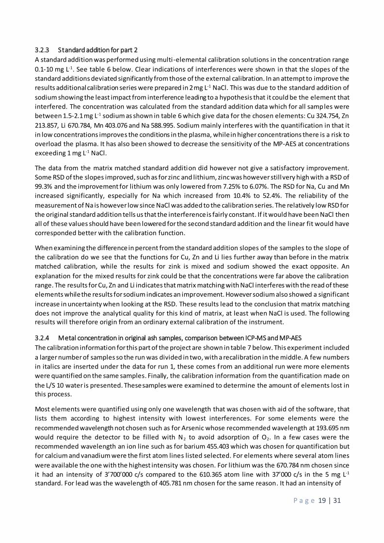
The calibration information for this part of the project are shown in table 7 below. This experiment included

a larger number of samples so the run was divided in two, with a recalibration in the middle. A few numbers

in italics are inserted under the data for run 1, these comes f rom an additional run were more elements

were quantified on the same samples. Finally, the calibration information from the quantification made on

the L/S 10 water is presented. These samples were examined to determine the amount of elements lost in this process.

Most elements were quantified using only one wavelength that was chosen with aid of the software, that

lists them according to highest intensity with lowest interferences. For some elements were the

recommended wavelength not chosen such as for Arsenic whose recommended wavelength at 193.695 nm

would require the detector to be filled with N2 to avoid adsorption of O2. In a few cases were the

recommended wavelength an ion line such as for barium 455.403 which was chosen for quantification but

for calcium and vanadium were the first atom lines listed selected. For elements where several atom lines

were available the one with the highest intensity was chosen. For lithium was the 670.784 nm chosen since

it had an intensity of 3’700’000 c/s compared to the 610.365 atom line with 37’000 c/s in the 5 mg L-1 standard. For lead was the wavelength of 405.781 nm chosen for the same reason. It had an intensity of

P a g e 20 | 31

Table 6: Results from the standard addition for part 2, the concentrations are given in mg L-1 for all elements except for Li which is given in µg L-1. These concentrations

are calculated from the standard addition functions. The samples are digests from ash provided by SAKAB AB. The abbreviations used mean as follows; A: digestion with

concentrated HNO3, B: digestion with aqua regia, C: digestion with 18.2 MΩ water. Samples 1-3 are replicates from the same batch of ash while the sample labelled 4 is a method blank. NORMAL

Cu 324.754 Zn 213.857 Li 670.784 Mn 403.076 Na 588.995

[Cu]

mg L-1

% diff.

slope

r2 [Zn]

mg L-1

% diff.

slope

r2 [Li]

µg L-1

% diff.

slope

r2 [Mn]

mg L-1

% diff.

slope

r2 [Na]

mg L-1

% diff.

slope

r2

1A 2.15 52.1 0.9916 1298 98.2 0.089 42.3 16.6 0.998 1.603 51.7 0.9903 1.6382 50.3 0.9993

1B 1.55 37.6 0.9876 35.5 35.4 0.3122 24.4 10.2 0.9999 1.496 46.9 0.9993 1.6111 45.0 0.9996 1C 1.30 47.7 0.9886 275 92.5 0.4209 16.7 11.0 0.9993 0.251 49.4 0.9992 1.5587 46.5 1 2A 1.77 43.2 0.9885 10.2 -119.6 0.9898 7.1 -2.0 0.9957 1.377 46.2 0.9722 1.5697 44.4 0.9686 3A 2.00 53.1 0.9794 137 84.0 0.4011 18.3 25.3 0.9981 1.581 56.2 0.9968 2.1460 48.6 0.9803 4A 0.01 45.9 0.9997 0.22 51.6 0.9964 0.8 6.4 1 0.007 50.1 0.9994 0.1463 47.9 0.9957

C0.1 0.07 slope r2 0.03 slope r2 73 slope r2 0.0819 slope r2 o.r. slope r2

C1 0.89 82822 0.9998 0.74 7136 1 896 778774 0.9998 0.8616 31770 1 5.8813 220994 0.9995

RSD 10.8% RSD 137% RSD 7.25% RSD 4.23% RSD 10.4%

MATRIX MATCHED Cu 324.754 Zn 213.857 Li 670.784 Mn 403.076 Na 588.995

[Cu] mg L-1

% diff. slope

r2 [Zn] mg L-1

% diff. slope

r2 [Li] µg L-1

% diff. slope

r2 [Mn] mg L-1

% diff slope

r2 [Na] mg L-1

% diff slope

r2

1A 2.30 57.1 0.99 274 108.8 0.3818 38.4 53.2 0.9986 1.95 59.9 0.9975 4.32 41.2 0.9892 1B 1.89 49.0 0.8851 372 93.5 0.0274 20.7 49.8 0.9994 1.89 57.8 0.9751 2.33 -39.2 0.8589 1C 1.21 50.0 0.9969 27.4 22.3 0.9534 27.5 53.2 0.9998 0.293 56.3 0.998 1.83 32.9 0.9994 2A 1.62 37.3 0.9899 14.1 -67.7 0.9992 13.8 47.7 0.9988 1.32 45.8 0.9973 1.62 9.2 0.9945 3A 2.43 59.6 0.9874 27.1 10.7 0.6678 51.0 55.9 0.9951 2.55 70.4 0.9772 12.8 81.5 0.2353

4A 0.002 51.9 0.9997 0.012 47.1 0.9988 1.5 50.6 1 0.0018 54.0 1 0.446 18.5 0.9994

C0.1 0.088 slope r2 0.088 slope r2 90 slope r2 0.103 slope r2 0.065 slope r2 C1 0.973 90813 1 1.090 5378.1 0.9997 924 771297 0.9999 0.906 31691 0.9999 1.26 206893 0.9989 RSD 15.8% RSD 99.3% RSD 6.07% RSD 18.9% RSD 52.4%

P a g e 21 | 31

15’000 c/s in the 5 mg L-1 standard which was higher than the 6000 and 8000 c/s in the 368.346 and 283.305 nm atom lines, respectively.

Table 7: Wavelengths and mass numbers quantified, values in italics is from another

run. Regressions with an L represent l inear calibration fi t while R represent the rational calibration model in the software.

Sample run part 1

Normal calibration

Sample run part 2

Normal calibration L/S 10

% error

r2 % error

r2 % error

r2

Al 396.152 10 L: 0.99993 10 0.99999 10 L: 0.99814 As 234.984 5 R: 0.99994 7 R: 0.99896 25 R: 0.99942 Ba 455.403 10 L: 0.99996 10 0.99928 7 R: 0.99991 Ba 553.548 5 L: 0.99994 10 0.99998 12 L: 0.99707 Ca 422.673 20 L: 0.99971 - - - - Cd 228.802 10 L: 0.99880 5 0.99969 10 R: 0.99887 Cr 425.433 10 L: 0.99993 10 0.99999 10 L: 0.99814 Cu 324.754 5 L: 0.99992 10 0.99962 10 R: 0.99913 K 766.491 25 L: 0.99995 - - - - Fe 371.993 10 L: 0.99998 16 0.99989 14 L: 0.99898 Li 610.365 7 L: 0.99998 10 0.99996 10 L: 0.99731 Li 670.784 7 L: 0.99992 11 0.99992 20 R: 0.99996 Mn 403.076 5 L: 0.99998 11 0.99978 10 L: 0.99808 Na 588.995 30 L: 0.99958 - - 6 L: 0.99865 Ni 352.454 5 L: 0.99985 10 0.99987 10 L: 0.99955 Pb 283.305 25 L: R: 0.99992 11 0.99980 - - Pb 368.346 5 L: 0.99999 15 0.99982 uncal L: 0.99934 Pb 405.781 5 L: 0.99999 16 0.99977 12 L: 0.99905 V 437.923 30 R:0.99995 - - - - Zn 213.857 10 L: 0.99952 5 0.99870 5 R: 0.99995

The data in table 8 consist of the complete calculated concentrations in mg g-1 ash for the determined

elements. The data in this table are given for the quantification made with conventional external calibration

since the matrix matching (section 3.2.3) gave no improvement. The data include digestions with aqua regia

since the evaluation of digestion methods (section 3.2.3) proved this to give the best results for both

instruments. This approach means that the interferences found in the standard addition (section 3.2.3) still

has not been successfully dealt with. However, when comparing the results from the MP-AES with those

from the ICP-MS no proof is found that this interference has altered the quality of the quantification.

The results from the MP-AES and ICP-MS are in fact surprisingly similar, some elements have almost identical

concentrations such as samples 1 and 3 for barium which is given as 1.26 mg g-1 in the MP-AES and 1.28 mg

g-1 in the ICP-MS. The results for nickel are even closer with values for sample 1 given as 0.68 in both

instruments, although the most sensitive atom line in the MP-AES should have been chosen. Other elements

that differ with less than 0.5 mg g-1 between the instruments are Cr, Cu, Fe, Mn and Pb. Zinc differs with a

few mg between the techniques but when regarding the incredibly high concentration of this element this

difference can be considered minor. The elements Ca, K, Li and Na were not quantified with the ICP-MS and

cannot be compared and vanadium and arsenic were the only element not being possible to quantify with

the MP-AES. Vanadium was under the detection limits while the inadequate result for arsenic was due to

this atom line being highly affected of interferences from beryllium and iron. The atom line also has a low

P a g e 22 | 31

sensitivity. The other elements differed less than 1 mg g-1 between the instruments except for cadmium which had one sample which differed with roughly 1.5 mg g-1.

All elements included were quantified in the samples, even if the amount of vanadium was very low (24 µg g-

1). The highest concentrations were found for zinc and calcium, the former with concentrations around 350

mg g-1 and the latter around 90 mg g-1. This mean that they together make up nearly half of the dry weight of

the ashes. Arsenic was around 45 mg g-1 in the ICP-MS but could not be detected by the MP-AES. The

concentration of iron was around 18 mg g-1 while several elements had concentrations of 10 ± 2 mg g-1 such

as Cu, K and Mn. Elements with concentrations of 5 ± 2 mg g-1 were Al, Cd, Cr, Na and Pb. Note that the main

reason the samples underwent 8 cycles of L/S 10 was to remove Na, meaning that the concentration of this

element was much higher from the beginning, which will be discussed further below. Finally , some elements was present in low concentrations such as Ba (1.3 mg g-1), Ni (0.7 mg g-1) and Li (0.1 mg g-1).

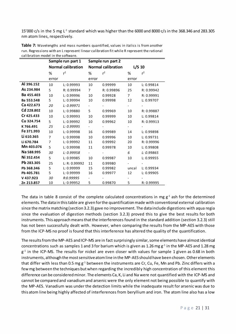
The concentration of sodium found to give a decrease in signal intensities (section 3.1.1) was 5 g L-1. To get

below this threshold the leaching out of the samples was controlled with electrical conductivity and

concentration of sodium in each sample with the MP-AES. The results from these measurements are shown

in figure 14. The highest concentration in the first cycle of L/S 10 was above the calibration range but a clear

resemblance is still visible between the measurement of conductivity and concentration that show an

inversely exponential relation between the amount of Na and the L/S cycle. The leachable amount of sodium

were between 2.2-2.4 mg g-1 ash, giving a concentration in the original samples around 10 mg g-1. This is

however far below the concentrations that affect the signal intensities adversely which rises a hypothesis

that this sort of matrix could be quantified without an L/S 10 pretreatment. Then the slight loss of elements

in the L/S 10 pretreatment could be avoided, as for Pb, Li and Cr which averagely lost 0.29, 0.1 and 0.05 mg

g-1 ash respectively. The losses for the other elements were in lower µg g -1 range and can be considered minor.

This experiment show that the MP-AES give comparable results to that of Ar-ICP-instruments, which

correspond with what has been shown in the literature [2], [3], [15], [19]. The MP-AES is therefore an

attractive alternative due to its significant economic benefit, easy handling and the increased safety and ruggedness of this instrument.

P a g e 23 | 31

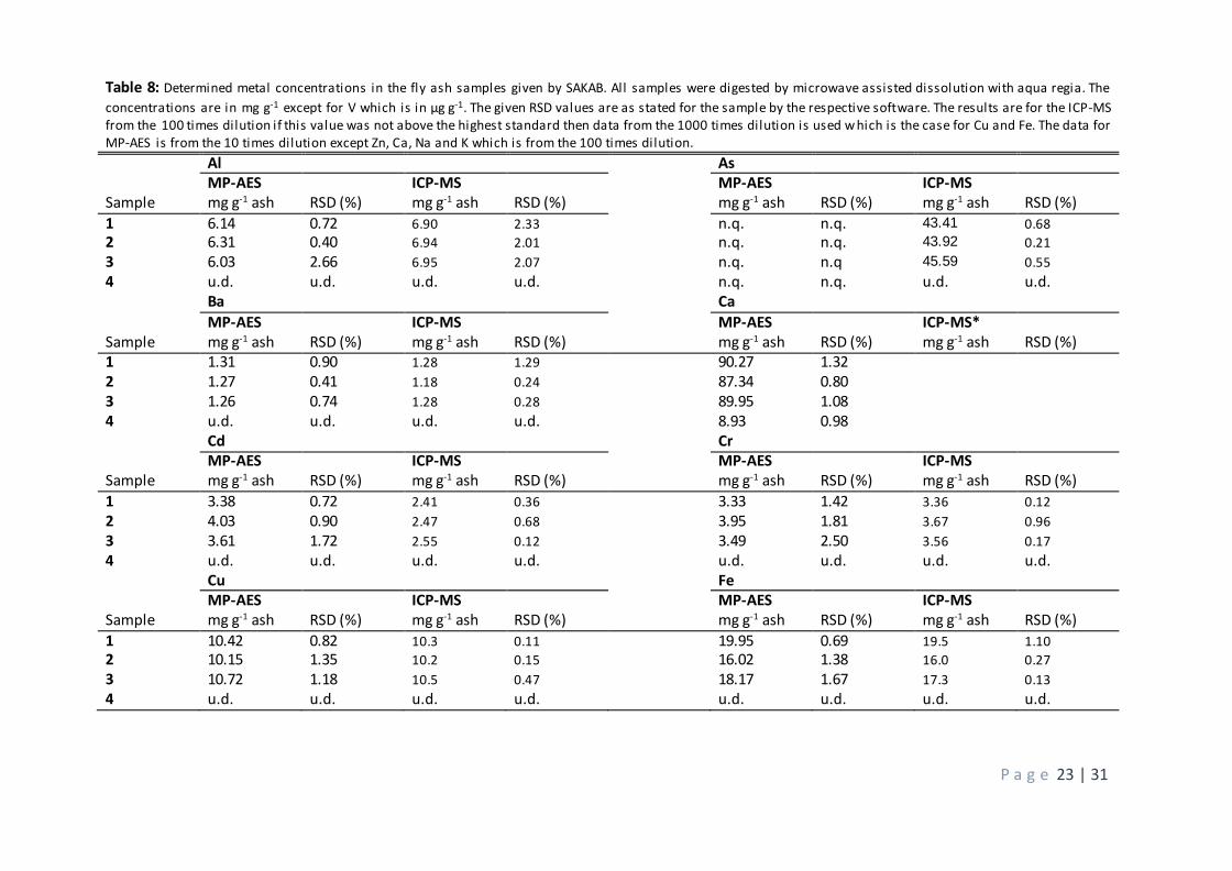
Table 8: Determined metal concentrations in the fly ash samples given by SAKAB. All samples were digested by microwave assisted dissolution with aqua regia. The

concentrations are in mg g-1 except for V which is in µg g-1. The given RSD values are as stated for the sample by the respective software. The results are for the ICP-MS from the 100 times dilution if this value was not above the highest standard then data from the 1000 times dilution is used w hich is the case for Cu and Fe. The data for MP-AES is from the 10 times dilution except Zn, Ca, Na and K which is from the 100 times dilution.

Al As MP-AES ICP-MS MP-AES ICP-MS Sample mg g-1 ash RSD (%) mg g-1 ash RSD (%) mg g-1 ash RSD (%) mg g-1 ash RSD (%)

1 6.14 0.72 6.90 2.33 n.q. n.q. 43.41 0.68

2 6.31 0.40 6.94 2.01 n.q. n.q. 43.92 0.21

3 6.03 2.66 6.95 2.07 n.q. n.q 45.59 0.55

4 u.d. u.d. u.d. u.d. n.q. n.q. u.d. u.d. Ba Ca

MP-AES ICP-MS MP-AES ICP-MS* Sample mg g-1 ash RSD (%) mg g-1 ash RSD (%) mg g-1 ash RSD (%) mg g-1 ash RSD (%) 1 1.31 0.90 1.28 1.29 90.27 1.32

2 1.27 0.41 1.18 0.24 87.34 0.80

3 1.26 0.74 1.28 0.28 89.95 1.08

4 u.d. u.d. u.d. u.d. 8.93 0.98

Cd Cr MP-AES ICP-MS MP-AES ICP-MS Sample mg g-1 ash RSD (%) mg g-1 ash RSD (%) mg g-1 ash RSD (%) mg g-1 ash RSD (%)

1 3.38 0.72 2.41 0.36 3.33 1.42 3.36 0.12

2 4.03 0.90 2.47 0.68 3.95 1.81 3.67 0.96

3 3.61 1.72 2.55 0.12 3.49 2.50 3.56 0.17

4 u.d. u.d. u.d. u.d. u.d. u.d. u.d. u.d. Cu Fe MP-AES ICP-MS MP-AES ICP-MS Sample mg g-1 ash RSD (%) mg g-1 ash RSD (%) mg g-1 ash RSD (%) mg g-1 ash RSD (%)

1 10.42 0.82 10.3 0.11 19.95 0.69 19.5 1.10 2 10.15 1.35 10.2 0.15 16.02 1.38 16.0 0.27 3 10.72 1.18 10.5 0.47 18.17 1.67 17.3 0.13 4 u.d. u.d. u.d. u.d. u.d. u.d. u.d. u.d.

P a g e 24 | 31

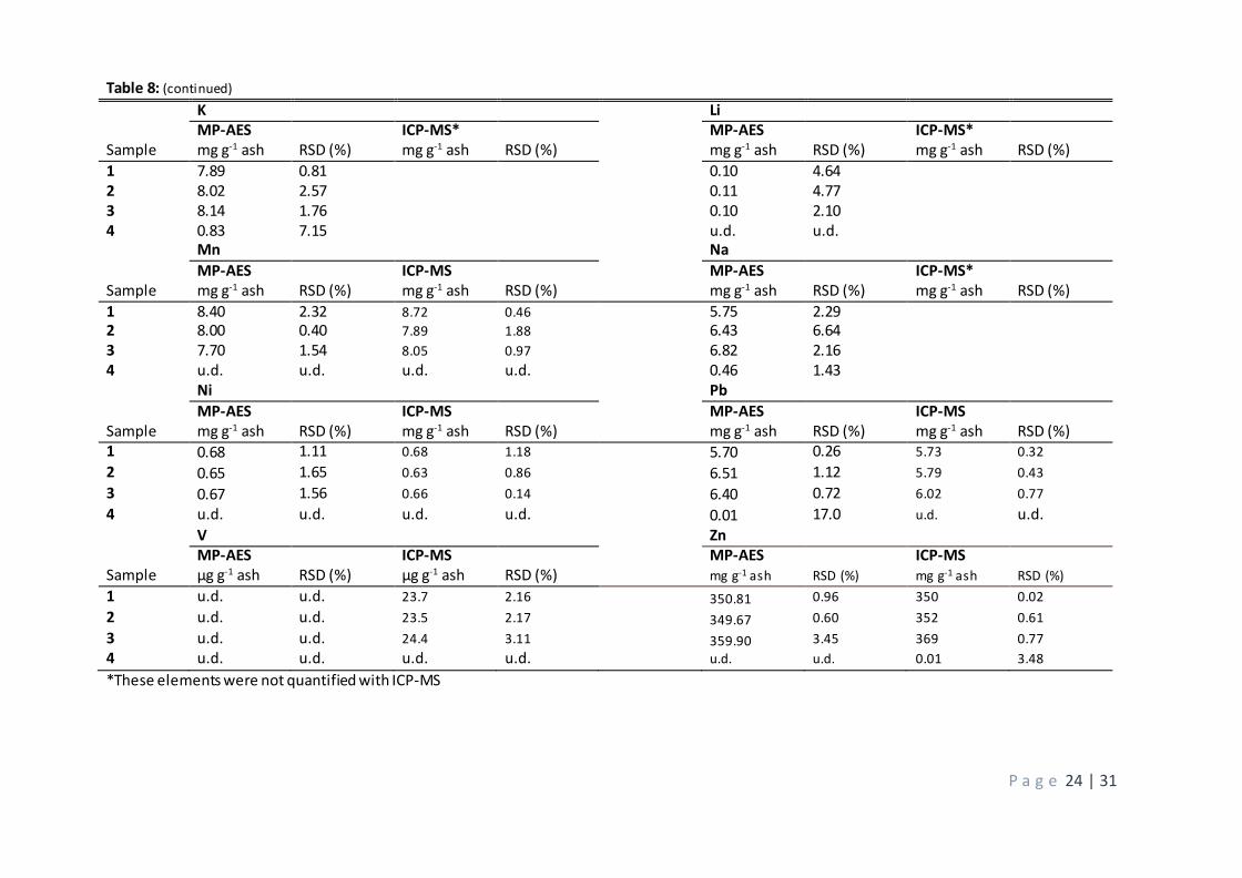
Table 8: (continued)

K Li MP-AES ICP-MS* MP-AES ICP-MS* Sample mg g-1 ash RSD (%) mg g-1 ash RSD (%) mg g-1 ash RSD (%) mg g-1 ash RSD (%)

1 7.89 0.81 0.10 4.64

2 8.02 2.57 0.11 4.77

3 8.14 1.76 0.10 2.10

4 0.83 7.15 u.d. u.d.

Mn Na

MP-AES ICP-MS MP-AES ICP-MS* Sample mg g-1 ash RSD (%) mg g-1 ash RSD (%) mg g-1 ash RSD (%) mg g-1 ash RSD (%)

1 8.40 2.32 8.72 0.46 5.75 2.29

2 8.00 0.40 7.89 1.88 6.43 6.64

3 7.70 1.54 8.05 0.97 6.82 2.16

4 u.d. u.d. u.d. u.d. 0.46 1.43

Ni Pb

MP-AES ICP-MS MP-AES ICP-MS Sample mg g-1 ash RSD (%) mg g-1 ash RSD (%) mg g-1 ash RSD (%) mg g-1 ash RSD (%) 1 0.68 1.11 0.68 1.18 5.70 0.26 5.73 0.32

2 0.65 1.65 0.63 0.86 6.51 1.12 5.79 0.43

3 0.67 1.56 0.66 0.14 6.40 0.72 6.02 0.77

4 u.d. u.d. u.d. u.d. 0.01 17.0 u.d. u.d.

V Zn MP-AES ICP-MS MP-AES ICP-MS Sample µg g-1 ash RSD (%) µg g-1 ash RSD (%) mg g-1 ash RSD (%) mg g-1 ash RSD (%)

1 u.d. u.d. 23.7 2.16 350.81 0.96 350 0.02

2 u.d. u.d. 23.5 2.17 349.67 0.60 352 0.61

3 u.d. u.d. 24.4 3.11 359.90 3.45 369 0.77

4 u.d. u.d. u.d. u.d. u.d. u.d. 0.01 3.48

*These elements were not quantified with ICP-MS

P a g e 25 | 31

Figure 14: Sample 1 -3 with respective electrical conductivity and intensity measurements. S1-3 int. is a based on the primary y-axis, intensity in c/s, while S1-3 cond. is based on the secondary y-axis, conductivity in mS/cm. The x-axis represent the L/S 10 round.

Figure 16: Results for ash samples after an L/S 10, before and after these samples were

treated with bark compost. The concentration in mg/L is shown on the y-axis and the

name of the element in question is shown on the x-axis. All samples has been adjusted for the dilution, including the control. A: Ash samples C…: Control samples.

Figure 15: Results for ash samples after an L/S 10, before and after these samples were treated with combusted waste ashes. The concentration in mg/L is shown on the y-axis and the name of the element in question is shown on the x-axis. All samples has been adjusted for the dilution, including the control. A: Ash samples C…: Control

samples.

P a g e 26 | 31

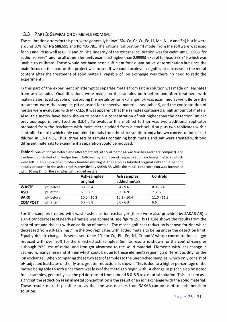
3.3 PART 3: SEPARATION OF METALS FROM SALT The calibration errors for this part were generally below 15% (Cd, Cr, Cu, Fe, Li, Mn, Ni, V and Zn) but it were

around 50% for Na 588.995 and Pb 405.781. The rational calibration fit model from the software was used

for Na and Pb as well as Cu, V and Zn. The linearity of the external calibration was for cadmium 0.99986, for

sodium 0.99974 and for all other elements examined higher than 0.99993 except for lead 368.346 which was

unable to calibrate. These would not have been sufficient for a quantitative determination but since the

main focus on this part of the project was to see if we could achieve a significant decrease in the metal

content after the treatment of solid material capable of ion exchange was there no need to redo the experiment.

In this part of the experiment an attempt to separate metals from salt in solution was made on leachates

from ash samples. Quantifications were made on the samples both before and after treatment with

materials believed capable of absorbing the metals by ion exchange, pH was examined as well. Before the

treatment were the samples pH adjusted for respective material, see table 9, and the concentration of

metals were evaluated with MP-AES. It was apparent that the samples contained a high amount of metals.

Also, this matrix have been shown to contain a concentration of salt higher than the detection limit in

previous experiments (section 3.2.4). To evaluate this method further was two additional replicates

prepared from the leachates with more metals added from a stock solution plus two replicates with a

controlled matrix which only contained metals from the stock solution and a known concentration of salt

diluted in 1% HNO3. Thus, three sets of samples containing both metals and salt were treated with two different materials to examine if a separation could be induced.

Table 9: Values for pH before and after treatment of solid material (waste ashes and bark compost). The

treatment consisted of pH-adjustment followed by addition of respective ion exchange material which

were left in an end-over-end rotary tumbler overnight. The samples labelled original only contained the metals prescent in the ash samples provided by SAKAB AB while the metal -concentration was increased with 10 mg L-1 for the samples with added metals. Ash-samples

original Ash samples added metals

Controls

WASTE ASH

pH before 8.1 - 8.4 8.4 - 9.6 8.0 - 8.4

pH after 6.9 - 7.2 6.7 - 6.9 7.3 - 7.5

BARK COMPOST

pH before 10.0 - 10.2 10.1 - 10.4 11.0 - 11.3

pH after 6.7 - 6.8 6.0 - 6.3 6.6

For the samples treated with waste ashes as ion exchanger (these were also provided by SAKAB AB) a

significant decrease of nearly all metals was apparent, see figure 15. This figure shows the results from the

control set and the set with an addition of metals. The most significant reduction is shown for zinc which

decreased from 9.0-12.2 mg L-1 in the two replicates with added metals to being under the detection limit.

Equally drastic changes is seen, see table 10, for Cu, Pb, Fe, Ni, Cr and V whose concentrations all got

reduced with over 90% for the enriched ash samples. Similar results is shown for the control-samples

although 20% less of nickel and iron got absorbed to the solid material. Elements with less change is

cadmium, manganese and lithium which could be due to these elements requiring a different acidity for the

ion exchange. When comparing these two sets of samples to the unenriched samples, which only consist of

pH-adjusted leachates of the fly ash, greater reductions is shown. This is due to a higher percentage of the

metals being able to sorb since there was less of the metals to begin with. A change in pH can also be noted

for all samples, generally has the pH decreased from around 8.0-8.5 to a neutral solution. This is taken as a

sign that the reduction seen in metal concentration is the result of an ion exchange with the solid material.

These results make it possible to say that the waste ashes from SAKAB can be used to sorb metals in

solution.

P a g e 27 | 31

The previous results can be compared with what was achieved with the second treatment of bark compost,

which is given in figure 16 and table 10. The results for this treatment were generally better than the ones

with ash for most elements, especially for cadmium which was reduced with around 90% for all systems in

this treatment compared to around 50% in the treatment with waste ashes. A greater reduction is also seen

for lithium, with a 66,6% reduction compared to 38,5% for the controlled matrix. . The results for Cu, Pb and

Fe were similar while Mn showed an increase in both samples containing ash with -55,2% and -74,3%

respectively, the control samples however still gave a reduction. This batch of compost has been examined

by Viktor Sjöberg [27] who found the same increase of manganese after treatment at a pH around 6.0. Thus,

this extra manganese is due to the pH getting low enough in these systems for manganese to release from

the bark compost. The pH for the control solutions never got below 6.7 which explains the difference. This

means that to avoid the increase of manganese in the solution when using bark compost more care needs to

be taken of the pH of the solution. Finally, when comparing the methods do we see that the treatment with

bark compost in most cases resolved in greater extent of metal separation from the salt with manganese as an exception.

Table 10: An average of the decrease in percent with RSD for examined metals after treatment with solid material capable of ion exchange. The samples were treated with respective solid material in an end -over-end

rotary tumbler overnight. The liquid solid ratios was 1 g per 10 mL water for the samples treated with waste ashes and 3g in 10 mL water for the samples treated with bark compost. Waste ash-treatment Bark compost-treatment

Controlled matrix

Ash original Ash

samples Controlled

matrix Ash original

Ash samples

Zn 100 ± 0 100 ± 0 100 ± 0 100 ± 0 100 ± 0 100 ± 0

Cd 46.8 ± 43.6 67.1 ± 8.6 57.1 ± 20.1 91.9 ± 1.8 92.5 ± 2.5 86.7 ± 3.5

Cu 97.6 ± 14 100 ± 0 98.8 ± 0.3 97.1 ± 0.5 100 ± 0 98.8 ± 0.3

Pb 95.5 ± 6.7 100 ± 0 94.4 ± 1.7 94.9 ± 0.6 99.4 ± 0.1 93.2 ± 1.6

Ni 73.3 ± 25.8 100 ± 0 96.3 ± 0.9 99.4 ± 0.9 100 ± 0 100 ± 0

Fe 73.6 ± 9.3 100 ± 0 90.4 ± 3.8 76.2 ± 5.0 100 ± 0 92.5 ± 2.1

Cr 95.1 ± 7.3 100 ± 0 100 ± 0.0 100 ± 0 100 ± 0 100 ± 0

V 92.6 ± 4.0 100 ± 0 100 ± 0.1 100 ± 0. 100 ± 0 100 ± 0

Mn 51.6 ± 8.1 49.0 ± 12.8 37.3 ± 54.9 34.3 ± 3.9 -55.2 ± 38.3 -74.3 ± 58.2

Li 38.5 ± 0.1 25.1 ± 8.9 8.4 ± 199.8 66.6 ± 1.5 37.0 ± 15.7 28.3 ± 56.7

A final note should be taken to the concentration of sodium, which after the treatment with solid material

greatly exceeding the calibration range meaning that there still was a high concentration of salt in the

samples. This mean that we have successfully separated most metals from the salt, although further method

optimization will be needed for manganese. The high concentration of sodium which exceeded the highest

standard of 10 mg L-1 could as discussed in section 3.1.1 be over the range of what the machine can handle

without loss of sensitivity but it was necessary to quantify the samples in this dilution due to the low

concentration of analytes. These results thus indicates that it is possible to clean the salt from the more

hazardous metals which opens up for the possibility to reuse the ashes as for example road salt. Further

research must however be taken with more elements such as arsenic which we found the ashes to have a high concentration of (section 3.2.4) before it is possible to say that this method will be sufficient.

P a g e 28 | 31

4 CONCLUSIONS

Conclusions drawn in this project are as follows:

The MP-AES is well suited for heavy matrices although the sensitivity will go down in matrices exceeding 5 g L-1 NaCl.

It has also been shown that the results from the MP-AES correspond well with the results achieved from the ICP-MS in this type of matrix.

Finally, the attempt to separate metals from salt with the help of bark compost and waste ashes

gave a positive outcome.

It is therefore possible to state that the MP-AES is an excellent replacement — to a greatly reduced

cost — for the ICP-MS to quantify matrices high in salt, as well as stating that the examined ashes could be reused.

5 ACKNOWLEDGMENTS

SAKAB AB and Thomas von Kronhelm is thanked for providing the samples examined in this project and

thanks go to Örebro University for the lending of equipment and resources required to perform this work.

I’m grateful to Viktor Sjöberg for his work with the ICP-MS to give me comparable data, and for the support

granted in the lab. Special thanks also goes to my supervisor Stefan Karlsson for guiding and helping me

every step of this project. Thanks also goes to Mattias Bäckström in his work of correcting it. Finally, I want a kind note to go to my classmates for all the late hours of exchanging advice and comfort.

P a g e 29 | 31

6 REFERENCES

[1] SAKAB, “Detaljerad information förbränning.” [Online]. Available: http://www.sakab.se/sv/behandling-av-avfall/forbranning-av-avfall/detaljerad-information-forbranning. [Accessed: 02-Apr-2015].

[2] S. Karlsson, V. Sjöberg, and A. Ogar, “Comparison of MP AES and ICP -MS for analysis of principal and selected trace elements in nitric acid digests of sunflower (Helianthus annuus).,” Talanta, vol. 135, pp. 124–32, Apr. 2015.

[3] Kamala C T, Balaram V, Dharmendra V, Satyanarayanan M, Subramanyam K S V, and Krishnaiah A, “Application

of microwave plasma atomic emission spectrometry (MP-AES) for environmental monitoring of industrially contaminated sites in Hyderabad city.,” Environ. Monit. Assess., vol. 186, no. 11, pp. 7097–113, Nov. 2014.

[4] Perkin Elmer incorporation, “The 30-minute guide to ICP-MS.” Waltham, USA, 2011.

[5] Agilent technologies, The Principles of ICP-MS. Agilent technologies, 2009.

[6] Agilent technologies, OneNeb - the Universal Nebulizer for ICP-OES and MP-AES. Agilent technologies, 2013.

[7] Agilent technologies, 4100 MP-AES Technology Video. Agilent technologies, 2011.

[8] A. Technologies, 4100 MP-AES web demo. Agilent technologies, 2013.

[9] R. D. Satzger and T. W. Brueggemeyer, “Preliminary Investigation of a Tangential Flow Torch with Coupling Probe Injector for Helium Microwave Induced Plasma Mass Spectrometry,” Mikrochim. Acta, pp. 239–246, 1989.

[10] P. Liang and A. Li, “Determination of arsenic by continuous hydride generation with direct introduction into an O 2 -argon microwave plasma torch atomic emission spectrometer,” Fresemius J Anal Chem, pp. 418–420, 2000.

[11] M. C. García, M. Varo, and P. Martínez, “Excitation of Species in an Expanded Argon Microwave Plasma at Atmospheric Pressure,” Plasma Chem. Plasma Process., vol. 30, no. 2, pp. 241–255, Jan. 2010.

[12] M. Baeva, X. Luo, J. H. Schafer, J. Uhlenbusch, and Z. Zhang, “Experimental and Theoretical Studies of a Pulsed Microwave Excited Ar / CF 4 Plasma,” Plasma Chem. Plasma Process., vol. 18, no. 4, pp. 429–446, 1998.

[13] S. Takahashi and T. Fujii , “Direct Mass Spectrometric Study of the Ionic Species Content of a C2HCl3/He/O2 Microwave Discharge Plasma,” Plasma Chem. Plasma Process., vol. 27, no. 5, pp. 517–528, Jul. 2007.

[14] C. Lalo, L. Deson, C. Cerveau, and R. I. Ben-Aim, “Air Microwave-Induced Plasma: Detection of NO in the Post-Discharge Using an ArF Laser,” Plasma Chem. Plasma Process., vol. 13, no. 2, pp. 351–364, 1993.

[15] W. Li, P. Simmons, D. Shrader, T. J. Herrman, and S. Y. Dai, “Microwave plasma -atomic emission spectroscopy as a tool for the determination of copper, iron, manganese and zinc in animal feed and fertil izer.,” Talanta, vol. 112, pp. 43–8, Aug. 2013.

[16] G. Heltai, B. Fehér, and M. Horváth, “Coupling of microwave induced plasma optical emission spectrometry with HPLC separation for speciation analysis of Cr(III)/Cr(VI),” Chem. Pap., vol. 61, no. 6, pp. 15–18, Jan. 2007.

[17] H. Matusiewicz, “A microwave plasma cavity assembly for atomic emission spectrometry.,” Anal. Bioanal. Chem., vol. 355, no. 5–6, pp. 623–5, Jul. 1996.

P a g e 30 | 31

[18] R. I. Pereiro and C. a. Díaz, “Speciation of mercury, tin, and lead compounds by gas chromatography with microwave-induced plasma and atomic-emission detection (GC–MIP–AED),” Anal. Bioanal. Chem., vol. 372, no. 1, pp. 74–90, Dec. 2001.

[19] V. Balaram, D. Vummiti, P. Roy, C. Taylor, P. Kar, A. K. Raju, and K. Abburi, “Determination of precious metals in

rocks and ores by microwave plasma-atomic emission spectrometry for geochemical prospecting studies,” Curr. Sci., vol. 104, no. 9, pp. 1207–1215, 2013.

[20] T. Hettipathirana, “Determination of metals in industrial wastewaters by microwave plasma - atomic emission spectrometry Application note.” Agilent technologies, Melbourne, Australia, 2011.

[21] “Optimization of method conditions for high matrix samples using the Agil ent Technical Overview.” Agilent technologies, Melbourne, Australia, 2014.

[22] M. Wiedenbeck, L. P. Bédard, R. Bugoi, M. Horan, K. Linge, S. Merchel, L. F. G. Morales, D. Savard, a. K. Souders,

and P. Sylvester, “GGR Biennial Critical Review: Analytical Developments Since 2012,” Geostand. Geoanalytical Res., vol. 38, no. 4, pp. 467–512, Dec. 2014.

[23] a. P. Khokhotva, “Adsorption of heavy metals by a sorbent based on pine bark,” J. Water Chem. Technol., vol. 32, no. 6, pp. 336–340, 2010.

[24] S. Karlsson, “Personal comment.” Örebro university, Örebro, sweden.

[25] A. Langford, J. Dean, R. Reed, D. Holmes, J. Weyers, and A. Jones, “Infrared and raman spectroscopy,” in Practical skills in forensic science, 2nd ed., Edinburgh, England: Pearson Education Limited, 2010.

[26] A. Gril l , “Dielectrics for Chip Interconnects Prepared by PECVD,” Annual Review of Materials Research, vol. 39,

no. 1. Supplemental Material: Annu. Rev. Mater. Res . 2009. 39:49-69 doi: 10.1146/annurev-matsci-082908-145305 Porous, pp. 49–69, 2009.

[27] P. Viktor Sjöberg, “Personal comment.” Örebro university, Örebro, sweden.