1

Paper 1400-2015

Validation and monitoring of PD models for low default portfolios using PROC MCMC

Machiel Kruger Centre for Business Mathematics and Informatics

North-West University, South Africa

ABSTRACT

A bank that wants to use the Internal Ratings Based (IRB) methods to calculate minimum Basel capital requirements have to calculate default probabilities (PDs) for all their obligors. Supervisors are mainly concerned about the credit risk being underestimated. For high quality exposures or groups with an insufficient number of obligors, calculations based on historical data may not be sufficiently reliable due to infrequent or no observed defaults. In an effort to solve the problem of default data scarcity, modelling assumptions are made and to control the possibility of model risk, a high level of conservatism is applied. Banks, on the other hand, are more concerned about PDs that are too pessimistic, since this has an impact on their pricing and economic capital. In small samples or where we have little or no defaults, the data provide very little information about the parameters of interest. The incorporation of prior information or expert judgment and using Bayesian parameter estimation can potentially be a very useful approach in a situation like this. Using PROC MCMC, we will show that a Bayesian approach can serve as a valuable tool for validation and monitoring of PD models for low default portfolios (LDPs). We will cover cases ranging from single period, zero correlation and zero observed defaults to multi-period, non-zero correlation and with few observed defaults.

INTRODUCTION

In terms of the Basel II framework, a bank that wants to use the Internal Ratings Based (IRB) methods to calculate minimum capital requirements have to calculate default probabilities (PDs) for all their obligors.

These PD models are usually based on historical data covering a period of five years. To estimate and validate the accuracy of these models a bank has to have to access to enough default data:

Basel §501: “Banks must regularly compare realised default rates with estimated PDs for each grade and be able to demonstrate that the realised default rates are within the expected range for that grade. .... Such comparisons must make use of historical data that are over as long a period as possible. The methods and data used in such comparisons by the bank must be clearly documented by the bank. This analysis and documentation must be updated at least annually.”

This means that banks has to compare their PD estimates and realized default rates at single grade level.

Basel §504: “Banks must have well-articulated internal standards for situations where deviations in realised PDs, LGDs and EADs from expectations become significant enough to call the validity of the estimates into question. These standards must take account of business cycles and similar systematic variability in default experiences. Where realised values continue to be higher than expected values, banks must revise estimates upward to reflect their default and loss experience.”

For high quality exposures or groups with a small number of obligors, calculations based on historical data may not be sufficiently reliable due to infrequent or no observed defaults. In an effort to solve the problem of default data scarcity, modelling assumptions are made and to control for the possibility of model risk, a high level of conservatism is applied. Although the supervisor is mainly concerned about the credit risk being under estimated, the bank is concerned about PDs that are too pessimistic, since this has an impact on their pricing and economic capital.

2

Any bank needs to determine the most appropriate methodology to calculate model accuracy for low default portfolios as this determines the Through the Cycle Probability of Default (TTC PD) level. The TTC PD drives RWA and as such it is important to have the correct PD level to ensure the regulatory capital is adequate.

Currently the “Pluto and Tasche” (Pluto and Tasche, 2006) approach is often used by banks to validate and monitor their LDP PD models. Since the proposal of Pluto and Tasche in 2006, other approaches have also been reported in the literature.

LITERATURE REVIEW

Although a number of possible approaches have been proposed in the literature, there is no consensus among academics or practitioners on which method is the most appropriate for predicting PDs for LDPs. In this paper we are, however, concerned with the validation and monitoring of LDP PD models. The question that we try to answer is:

Which methodology is the most appropriate methodology to validate and monitor a TTC PD model accuracy in the case of low default portfolios?

After an initial literature survey was done, we found that (see for example (Blümke, 2012)):

Some of the models need at least some defaults and is not applicable to no-default portfolios.

Some of the models are only single period.

The scarcity of default data makes back testing very difficult if not impossible.

Most of the available models are used for PD estimation and give no guidance on how to validate PD model.

The investigation into possible approaches and the selection of applicable methodologies was largely guided by the following assumptions.

Assumptions

The obligors in the portfolio are ranked according their riskiness and that the rating or score of an obligor contains all the information around its risk profile.

All exposures/obligors in a specific rating class are homogeneous in terms of their risk profile.

Only the Through the Cycle Probability of Default (TTC PD) level has to be validated and monitored.

Each rating class has an assigned or estimated TTC PD for the period covered by the historical data.

Multi-period methodologies that can handle portfolios with zero and low defaults are preferred.

Conclusion of Literature Review

After reading a large number of papers (see References for full list of papers considered) it became clear that a Bayesian approach is the most appropriate approach. For example:

Kiefer (2009) argues that

"… uncertainty about the default probability should be modeled the same way as uncertainty about defaults - namely, represented in a probability distribution."

Tasche (2013) concludes that

"… Bayesian estimators computed as a means of the posterior distributions can serve as an alternative to the upper confidence bounds approach. Such an alternative is welcome because it makes the necessarily subjective choice of a confidence level redundant."

For this reason the following papers were studied in more detail and most of the techniques contained in them were implemented:

3

Dwyer D.W. (2007), The distribution of defaults and Bayesian model validation, Journal of Risk Model Validation, Vol. 1, Iss. 1, pp. 23-53

Tasche D. (2013), Bayesian estimation of probabilities of default for low default portfolios, Journal of Risk Management in Financial Institutions, Vol. 6, Iss. 3, pp. 302-326

Chang YP and CT Yu (2014), Bayesian confidence intervals for probability of default and asset correlation of portfolio credit risk, Computational Statistics, Vol. 29, Iss. 1-2, pp. 331-361

BAYESIAN APPROACH IN A NUTSHELL

In Bayesian analysis the following steps are followed:

1) A prior distribution, θ , for each of the parameters θ of interest is specified before data is

observed.

2) Given the observed data, (y), a statistical model θ|yp is chosen which describes the data

given the parameters.

3) Prior beliefs about the parameters are updated by combining information from the prior

distributions and the data to produce a posterior distribution, yp |θ :

.|

||,|

θθ

θθθθθθ

dyp

yp

yp

yp

yp

ypyp

NOTATION AND GENERAL MULTIPERIOD STATISTICAL MODEL

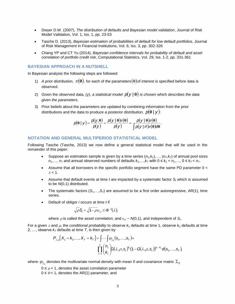
Following Tasche (Tasche, 2013) we now define a general statistical model that will be used in the remainder of this paper:

Suppose an estimation sample is given by a time series (n1,k1),…, (nT,kT) of annual pool sizes n1,…, nT and annual observed numbers of defaults k1,…,kT with 0 ≤ k1 < n1,…, 0 ≤ kT < nT.

Assume that all borrowers in the specific portfolio segment have the same PD parameter 0 <

< 1.

Assume that default events at time t are impacted by a systematic factor St which is assumed to be N(0,1) distributed.

The systematic factors (S1,…,ST) are assumed to be a first order autoregressive, AR(1), time series.

Default of obligor i occurs at time t if

, , 11 titS

where is called the asset correlation, and i,t ~ N(0,1), and independent of St.

For a given and , the conditional probability to observe k1 defaults at time 1, observe k2 defaults at time 2, …, observe kT defaults at time T, is then given by

,,,,,1,,

,,,,

1

1

111,

T

t

T

kn

t

k

t

t

t

TTT

ssdsGsGk

n

sskXkXP

ttt

where

denotes the multivariate normal density with mean 0 and covariance matrix

0 ≤ < 1, denotes the asset correlation parameter

0 ≤ < 1, denotes the AR(1) parameter, and

4

.,,

1

1

tt

ssG

MAXIMUM LIKELIHOOD ESTIMATION (MLE)

In cases where at least one default was observed one can use MLE to get estimates for the parameters (Tasche, 2013):

Given at least one default, one can assume that the systematic factors (S1,…,ST) are latent, i.e. not observable.

The remaining parameters, , and , can then be estimated using the following equation:

T

t

T

kn

t

k

t

t

t

T ssdsGsGk

nss ttt

1

11,,

,,,,1,,,,maxargˆ,ˆ,ˆ

The multiple integrals have to be estimated using Monte Carlo simulation. For this we need the

Cholesky decomposition of the correlation matrix , where

.

1

1

1

1

21

2

2

12

T

T

T

T

It is easy to verify that the Cholesky decomposition of , is given by the following lower triangular matrix (Wilde & Jackson, 2006):

.

111

0

11

001

0001

223221

222

2

TTT

We have implemented the MLE using PROC OPTMODEL and the SAS code is available from the author upon request.

For each of the Monte Carlo simulations, we generated 10 000 samples for the systematic factors (S1,…,ST).

For each of the examples below, we repeated the MLE a number of times, by changing the seed of the Monte Carlo simulations, to also get an estimate for the variance of the estimated parameters.

We also increased the sample size to 200 000 to check the sensitivity of the MLE, but the spread in the results did not improve significantly. For this reason and computational speed we have used a sample size of 10 000 to produce the results below.

CASE STUDIES

In what follows we give the details of applying the Bayesian approach to different business cases, including details on how the parameters were estimated.

Case I: Multi-period with zero defaults

In this case we cannot apply the Maximum Likelihood Estimation (MLE) to estimate the parameters of our general statistical model. We have to follow a Bayesian approach to analyze the data. Assuming

5

independence of , and , the joint posterior distribution is given by (Chang & Yu, 2014):

dsdddssyp

ssypysp

|,,|

|,,||,,,

To obtain the posterior distribution we us the SAS procedure, PROC MCMC, which is a general purpose Markov Chain Monte Carlo (MCMC) simulation procedure that is designed to fit Bayesian models.

In this report we will not go into the detail mechanics of the MCMC approach. The interested reader is referred to the paper “An Introduction to MCMC for Machine Learning” by Andrieu et. al (Andrieu, et. al, 2003).

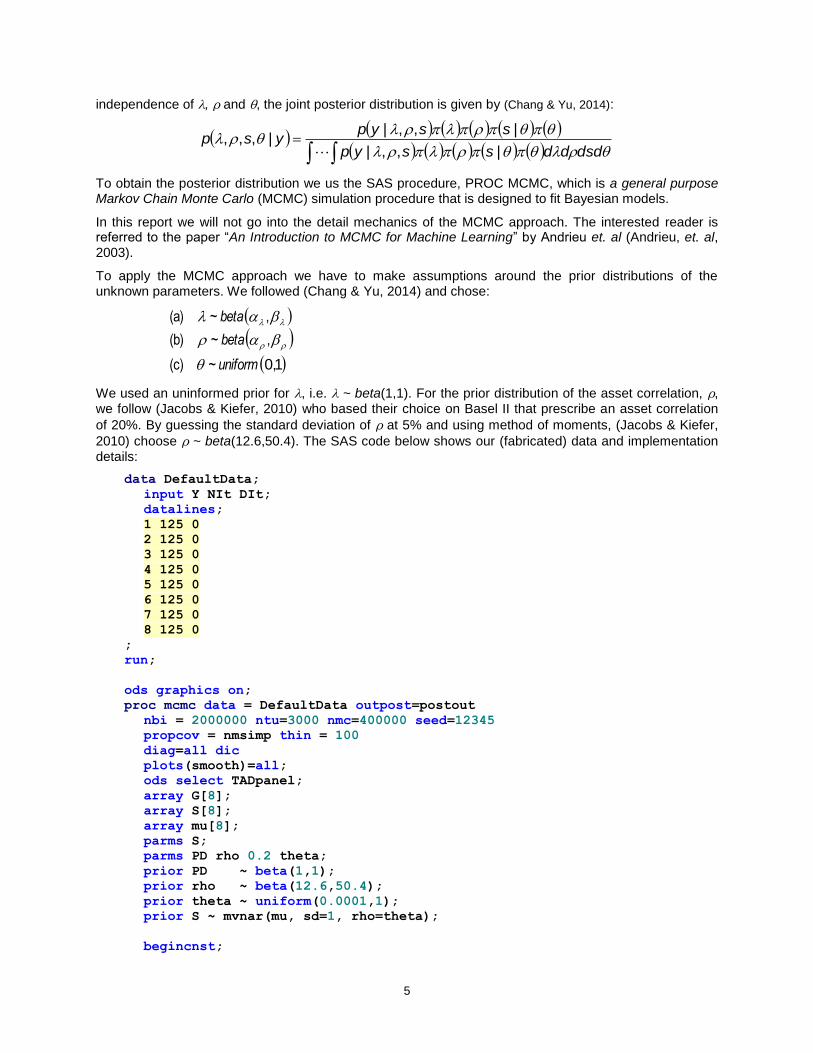
To apply the MCMC approach we have to make assumptions around the prior distributions of the unknown parameters. We followed (Chang & Yu, 2014) and chose:

10,~ (c)

,~ (b)

,~ (a)

uniform

beta

beta

We used an uninformed prior for , i.e. ~ beta(1,1). For the prior distribution of the asset correlation, , we follow (Jacobs & Kiefer, 2010) who based their choice on Basel II that prescribe an asset correlation

of 20%. By guessing the standard deviation of at 5% and using method of moments, (Jacobs & Kiefer,

2010) choose ~ beta(12.6,50.4). The SAS code below shows our (fabricated) data and implementation details:

data DefaultData;

input Y NIt DIt;

datalines;

1 125 0

2 125 0

3 125 0

4 125 0

5 125 0

6 125 0

7 125 0

8 125 0

;

run;

ods graphics on;

proc mcmc data = DefaultData outpost=postout

nbi = 2000000 ntu=3000 nmc=400000 seed=12345

propcov = nmsimp thin = 100

diag=all dic

plots(smooth)=all;

ods select TADpanel;

array G[8];

array S[8];

array mu[8];

parms S;

parms PD rho 0.2 theta;

prior PD ~ beta(1,1);

prior rho ~ beta(12.6,50.4);

prior theta ~ uniform(0.0001,1);

prior S ~ mvnar(mu, sd=1, rho=theta);

begincnst;

6

call zeromatrix(mu);

endcnst;

beginnodata;

do i = 1 to 8;

G[i] = probnorm((QUANTILE('NORMAL',PD,0,1) -

sqrt(rho)*S[i])/sqrt(1 - rho));

end;

endnodata;

model DIt ~ binomial(NIt,G[y]);

preddist outpred=pout nsim=10000;

run;

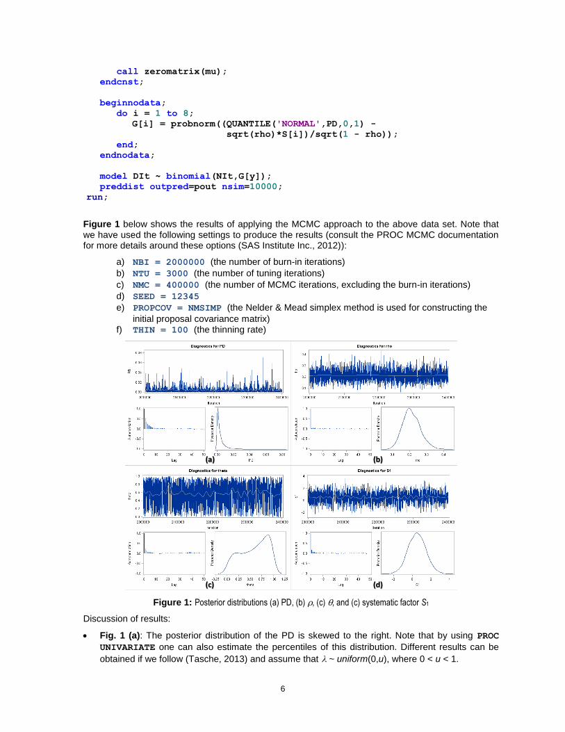
Figure 1 below shows the results of applying the MCMC approach to the above data set. Note that we have used the following settings to produce the results (consult the PROC MCMC documentation for more details around these options (SAS Institute Inc., 2012)):

a) NBI = 2000000 (the number of burn-in iterations)

b) NTU = 3000 (the number of tuning iterations)

c) NMC = 400000 (the number of MCMC iterations, excluding the burn-in iterations)

d) SEED = 12345

e) PROPCOV = NMSIMP (the Nelder & Mead simplex method is used for constructing the

initial proposal covariance matrix) f) THIN = 100 (the thinning rate)

Figure 1: Posterior distributions (a) PD, (b) , (c) , and (c) systematic factor S1

Discussion of results:

Fig. 1 (a): The posterior distribution of the PD is skewed to the right. Note that by using PROC

UNIVARIATE one can also estimate the percentiles of this distribution. Different results can be

obtained if we follow (Tasche, 2013) and assume that ~ uniform(0,u), where 0 < u < 1.

(a) (b)

(c) (d)

7

Fig. 1 (b): The posterior distribution of the asset correlation is close to symmetric. This is due to our specification of the prior beta(12.6,50.4). Given our assumptions on the prior distributions, this is in accordance with the fact zero defaults were observed. Again, different results can be

obtained if we follow (Tasche, 2013) and assume that ~ uniform(0,u), where 0 < u < 1.

Fig. 1 (c): Given our assumptions on the prior distributions for the parameters, the posterior

distribution of the AR parameter, , is in accordance with the fact zero defaults were observed.

Fig. 1 (d): Given zero observed defaults and that the general macro-economic environment was good, the posterior distribution of the systematic factor S1 has moved into a positive direction. Although not shown, this was also the case for S2,…,S8.

IMPORTANT NOTE: Given the fact that the data covers a period of only eight years, these results must be used/interpreted with great care. For example, if we were to change the prior distribution of

the AR parameter, , to uniform(-1,1) we will get different results.

The results in the above case (i.e. zero defaults) might seem to be unsatisfactory. One way to get a more conservative result is to assume a single default happened in one of the periods, let’s say in the period that has the smallest number of exposures. To then solve the problem, we have to follow the steps covered in the next section.

Case II: Multi-period with few defaults

The following default data set (Table 1, below) was derived from data reported in (Moody’s, 2014). First

the parameters , and , were estimated using MLE (described above).

Table 1: Investment Grade (IG) default data

Year Pool Size #Defaults

2000 2627 4

2001 2678 4

2002 2777 13

2003 2651 0

2004 2649 0

2005 2710 2

2006 2738 0

2007 2742 0

2008 2709 14

2009 2600 11

2010 2481 2

2011 2522 1

2012 2498 1

2013 2560 1

2014 2643 2

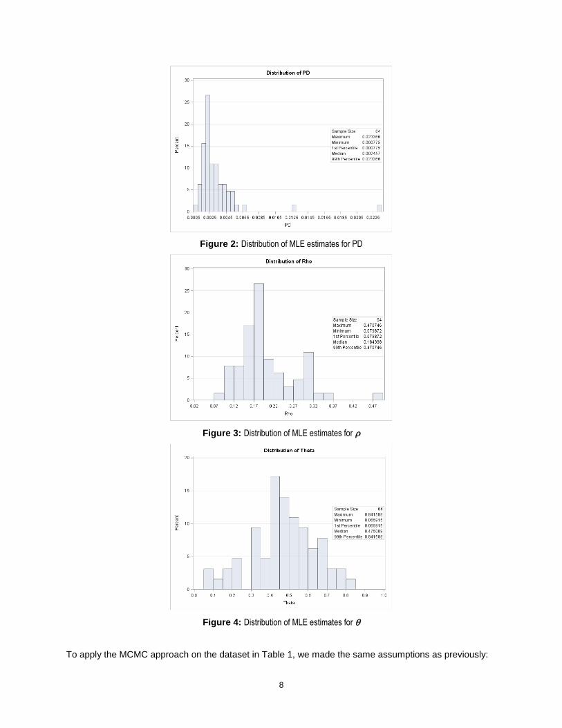
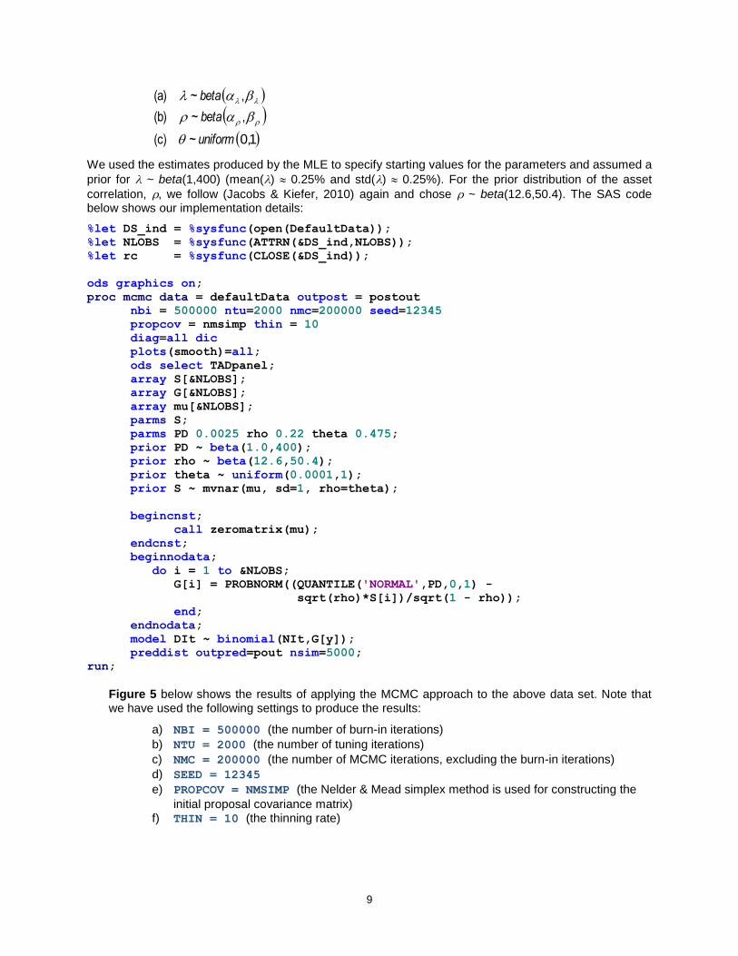
The results of the MLE estimation are shown in Figures 2 to 4 below:

Fig. 2 and 3 show the spread of the MLE estimates for PD and . This stresses that, to get reliable estimates for PD, one has to repeat the MLE a number of times using different seeds and then take the average or median of these estimates.

Fig.4 shows the spread of the MLE estimates for . Following (Tasche, 2013), we also

constrained the AR parameter, [0,1].

8

Figure 2: Distribution of MLE estimates for PD

Figure 3: Distribution of MLE estimates for

Figure 4: Distribution of MLE estimates for

To apply the MCMC approach on the dataset in Table 1, we made the same assumptions as previously:

9

10,~ (c)

,~ (b)

,~ (a)

uniform

beta

beta

We used the estimates produced by the MLE to specify starting values for the parameters and assumed a

prior for ~ beta(1,400) (mean() 0.25% and std() 0.25%). For the prior distribution of the asset

correlation, , we follow (Jacobs & Kiefer, 2010) again and chose ~ beta(12.6,50.4). The SAS code below shows our implementation details:

%let DS_ind = %sysfunc(open(DefaultData));

%let NLOBS = %sysfunc(ATTRN(&DS_ind,NLOBS));

%let rc = %sysfunc(CLOSE(&DS_ind));

ods graphics on;

proc mcmc data = defaultData outpost = postout

nbi = 500000 ntu=2000 nmc=200000 seed=12345

propcov = nmsimp thin = 10

diag=all dic

plots(smooth)=all;

ods select TADpanel;

array S[&NLOBS];

array G[&NLOBS];

array mu[&NLOBS];

parms S;

parms PD 0.0025 rho 0.22 theta 0.475;

prior PD ~ beta(1.0,400);

prior rho ~ beta(12.6,50.4);

prior theta ~ uniform(0.0001,1);

prior S ~ mvnar(mu, sd=1, rho=theta);

begincnst;

call zeromatrix(mu);

endcnst;

beginnodata;

do i = 1 to &NLOBS;

G[i] = PROBNORM((QUANTILE('NORMAL',PD,0,1) -

sqrt(rho)*S[i])/sqrt(1 - rho));

end;

endnodata;

model DIt ~ binomial(NIt,G[y]);

preddist outpred=pout nsim=5000;

run;

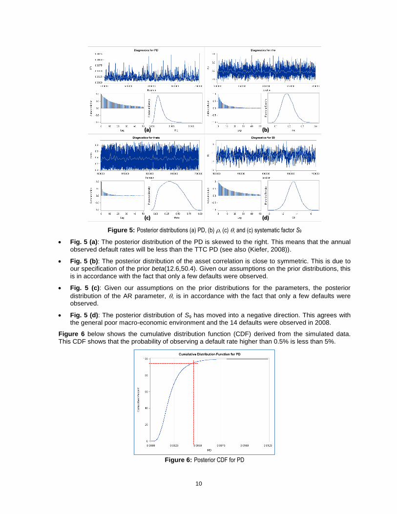
Figure 5 below shows the results of applying the MCMC approach to the above data set. Note that we have used the following settings to produce the results:

a) NBI = 500000 (the number of burn-in iterations)

b) NTU = 2000 (the number of tuning iterations)

c) NMC = 200000 (the number of MCMC iterations, excluding the burn-in iterations)

d) SEED = 12345

e) PROPCOV = NMSIMP (the Nelder & Mead simplex method is used for constructing the

initial proposal covariance matrix) f) THIN = 10 (the thinning rate)

10

Figure 5: Posterior distributions (a) PD, (b) , (c) , and (c) systematic factor S9

Fig. 5 (a): The posterior distribution of the PD is skewed to the right. This means that the annual observed default rates will be less than the TTC PD (see also (Kiefer, 2008)).

Fig. 5 (b): The posterior distribution of the asset correlation is close to symmetric. This is due to our specification of the prior beta(12.6,50.4). Given our assumptions on the prior distributions, this is in accordance with the fact that only a few defaults were observed.

Fig. 5 (c): Given our assumptions on the prior distributions for the parameters, the posterior

distribution of the AR parameter, , is in accordance with the fact that only a few defaults were observed.

Fig. 5 (d): The posterior distribution of S9 has moved into a negative direction. This agrees with the general poor macro-economic environment and the 14 defaults were observed in 2008.

Figure 6 below shows the cumulative distribution function (CDF) derived from the simulated data. This CDF shows that the probability of observing a default rate higher than 0.5% is less than 5%.

Figure 6: Posterior CDF for PD

(a) (b)

(c) (d)

11

Case III: Single-period with and without defaults

The joint distribution function for the probability of default, the aggregate shock and the number defaults for a single time period, t, is given by

PD Z

tt

kn

t

k

t

t

t

tt ddssfsGsGk

nkXZsPDP ttt

0

1 ,,,,,,

where f() is the density function of .

The posterior distribution of PD is given by (Dwyer, 2007: p. 34):

.

,,1,,

,,1,,

|1

0

0

ddssfsGsG

ddssfsGsG

kXPDP

tt

kn

t

k

t

PD

tt

kn

t

k

t

t

ttt

ttt

The above integrals have to be evaluated numerically. Note that if we assume that the PD has a uniform

prior distribution on the interval [0,1], then f() = 1 for all .

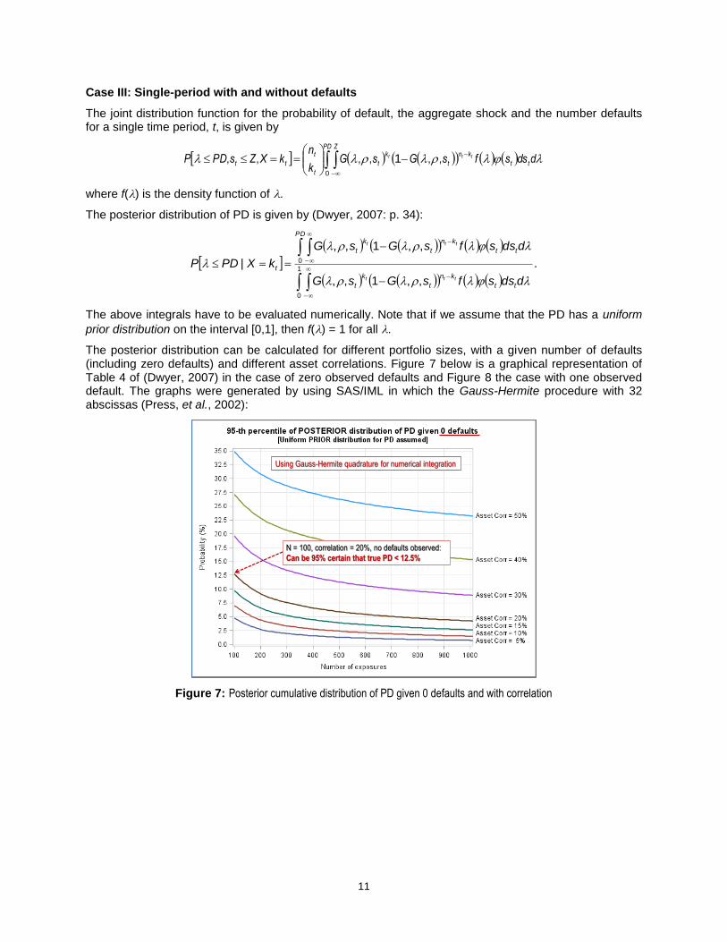
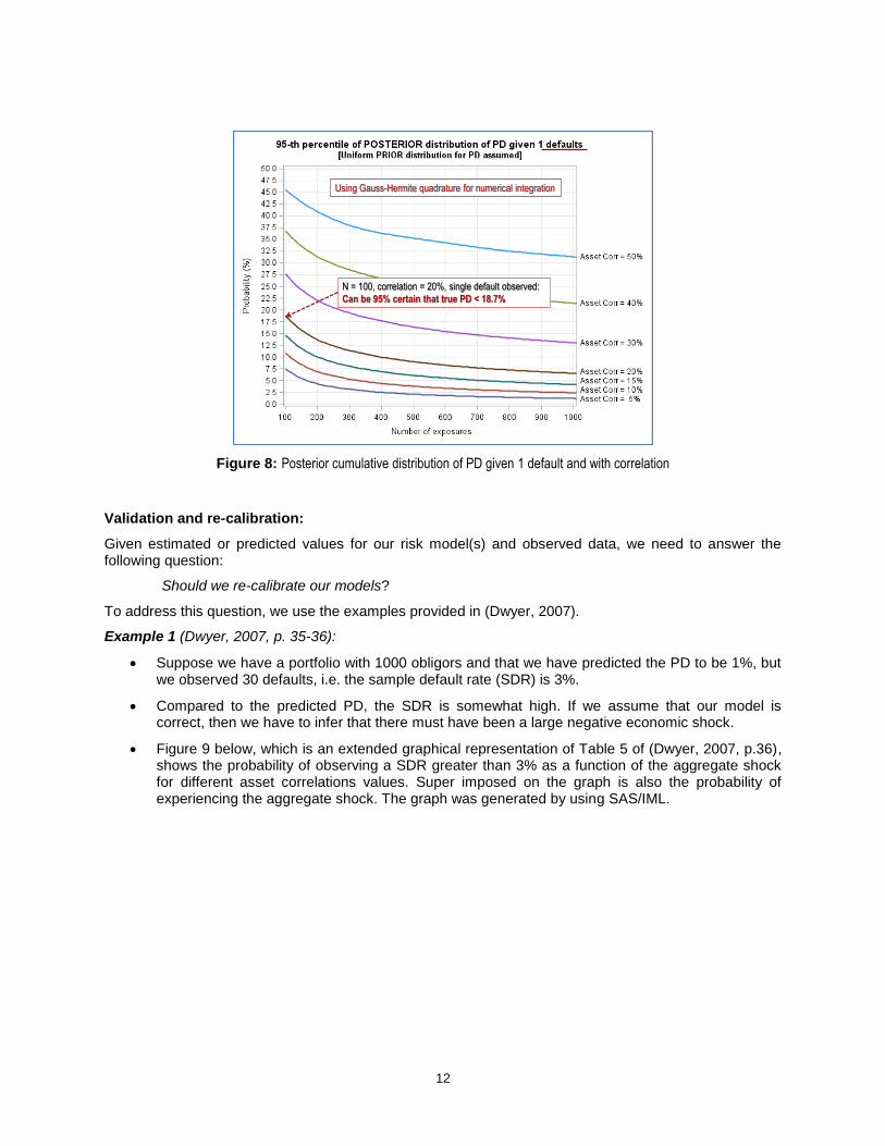
The posterior distribution can be calculated for different portfolio sizes, with a given number of defaults (including zero defaults) and different asset correlations. Figure 7 below is a graphical representation of Table 4 of (Dwyer, 2007) in the case of zero observed defaults and Figure 8 the case with one observed default. The graphs were generated by using SAS/IML in which the Gauss-Hermite procedure with 32 abscissas (Press, et al., 2002):

Figure 7: Posterior cumulative distribution of PD given 0 defaults and with correlation

Using Gauss-Hermite quadrature for numerical integration

N = 100, correlation = 20%, no defaults observed:

Can be 95% certain that true PD < 12.5%

12

Figure 8: Posterior cumulative distribution of PD given 1 default and with correlation

Validation and re-calibration:

Given estimated or predicted values for our risk model(s) and observed data, we need to answer the following question:

Should we re-calibrate our models?

To address this question, we use the examples provided in (Dwyer, 2007).

Example 1 (Dwyer, 2007, p. 35-36):

Suppose we have a portfolio with 1000 obligors and that we have predicted the PD to be 1%, but we observed 30 defaults, i.e. the sample default rate (SDR) is 3%.

Compared to the predicted PD, the SDR is somewhat high. If we assume that our model is correct, then we have to infer that there must have been a large negative economic shock.

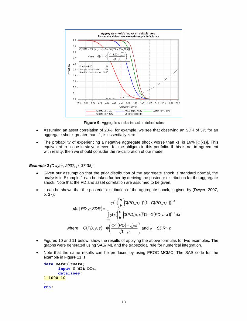
Figure 9 below, which is an extended graphical representation of Table 5 of (Dwyer, 2007, p.36), shows the probability of observing a SDR greater than 3% as a function of the aggregate shock for different asset correlations values. Super imposed on the graph is also the probability of experiencing the aggregate shock. The graph was generated by using SAS/IML.

Using Gauss-Hermite quadrature for numerical integration

N = 100, correlation = 20%, single default observed:

Can be 95% certain that true PD < 18.7%

13

Figure 9: Aggregate shock’s impact on default rates

Assuming an asset correlation of 20%, for example, we see that observing an SDR of 3% for an aggregate shock greater than -1, is essentially zero.

The probability of experiencing a negative aggregate shock worse than -1, is 16% [(-1)]. This equivalent to a one-in-six-year event for the obligors in this portfolio. If this is not in agreement with reality, then we should consider the re-calibration of our model.

Example 2 (Dwyer, 2007, p. 37-38):

Given our assumption that the prior distribution of the aggregate shock is standard normal, the analysis in Example 1 can be taken further by deriving the posterior distribution for the aggregate shock. Note that the PD and asset correlation are assumed to be given.

It can be shown that the posterior distribution of the aggregate shock, is given by (Dwyer, 2007, p. 37):

nSDRksPD

sPDG

dxxPDGxPDGk

nx

sPDGsPDGk

ns

SDRPDspknk

knk

and 1

,, where

,,1,,

,,1,,

,,|

1

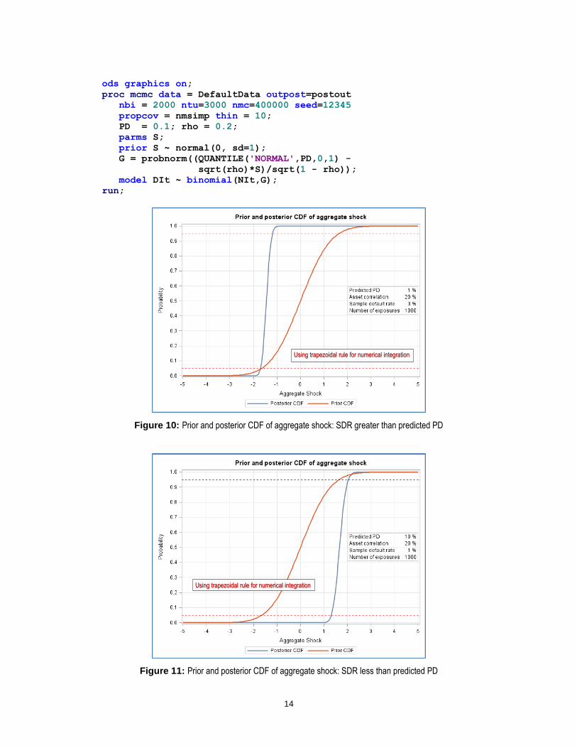
Figures 10 and 11 below, show the results of applying the above formulas for two examples. The graphs were generated using SAS/IML and the trapezoidal rule for numerical integration.

Note that the same results can be produced by using PROC MCMC. The SAS code for the example in Figure 11 is:

data DefaultData;

input Y NIt DIt;

datalines;

1 1000 10

;

run;

1 where

,,%31,,|%3

1 ssG

sGNNBinsSDRP

14

ods graphics on;

proc mcmc data = DefaultData outpost=postout

nbi = 2000 ntu=3000 nmc=400000 seed=12345

propcov = nmsimp thin = 10;

PD = 0.1; rho = 0.2;

parms S;

prior S ~ normal(0, sd=1);

G = probnorm((QUANTILE('NORMAL',PD,0,1) -

sqrt(rho)*S)/sqrt(1 - rho));

model DIt ~ binomial(NIt,G);

run;

Figure 10: Prior and posterior CDF of aggregate shock: SDR greater than predicted PD

Figure 11: Prior and posterior CDF of aggregate shock: SDR less than predicted PD

Using trapezoidal rule for numerical integration

Using trapezoidal rule for numerical integration

15

For the case in Figure 10, it follows that we are 95% sure that the aggregate shock is less than -1.16. The probability of this happening is 12%, i.e. 1-in-8-year event. This means that observing an SDR of 3% when our model has predicted a default rate of 1%, will only be consistent if we are at or close to the bottom of the credit cycle.

For the case in Figure 11, it follows that we are 95% sure that the aggregate shock is larger than

1.3. The probability of this happening is 10% [1-(1.3)], i.e. 1-in-10-year event. This means that observing an SDR of 1% when our model has predicted a default rate of 10%, will only be consistent if the macro-economic environment was pretty favorable, otherwise our model is too conservative and needs to be re-calibrated.

CONCLUSION

This paper showed that the Bayesian approach can serve as a valuable tool for validation and monitoring of PD models for LDPs. PROC OPTMODEL was used for the MLE of the multi-period statistical model and PROC MCMC was used to implement the Bayesian approach to show how the overall validation and monitoring process can be done in a very compact way, i.e. little programming effort is needed.

Future research could focus on the development of a process to formally incorporate expert opinion in PD modelling and validation.

REFERENCES

Andrieu C., N. de Freitas, A. Doucet and M. I. Jordan (2003), “An introduction to mcmc for machine learning”, Machine Learning, Vol. 50, 5-43

BBA, LIBA, and ISDA (2005), “Low Default Portfolios”,”Discussion paper, British Banking Association, London Investment Banking Association and International Swaps and Derivatives Association, Joint Industry Working Group

Benjamin N., C. Cathcart & K. Ryan (2006), “Low Default Portfolios: A Proposal for Conservative Estimation of Default Probabilities”, Discussion paper, Financial Services Authority

Blümke O. (2012), “Probability of default validation: a single-year and a multiyear methodology for the Basel framework”, The Journal of Risk Model Validation, Vol. 6, Iss. 2, 47–79

Chang YP. & CT. Yu (2014), “Bayesian confidence intervals for probability of default and asset correlation of portfolio credit risk”, Computational Statistics, Vol. 29, Iss. 1-2, 331-361

Clifford T., Sebestyen K. & A. Marianski (2013), “Low Default Portfolio (LDP) Modelling: Probability of Default (PD) Calibration Conundrum”, Credit Scoring and Credit Control XIII conference

Dwyer D.W. (2007), “The distribution of defaults and Bayesian model validation”, Journal of Risk Model Validation, Vol. 1, Iss. 1, 23-53

Dzidzevičiūtė L. (2012), “Estimation of Default Probability for Low Default Portfolios”, Ekonomika, Vol. 91 Iss. 1, 132-156

Forrest A. (2005), “Likelihood approaches to Low Default Portfolios”, Joint Industry Working Group Discussion Paper. Credit Research Center (CRC), University of Edinburgh

Frunza M. (2013), “Are Default Probability Models Relevant for Low Default Portfolios?”, Available at SSRN: http://ssrn.com/abstract=2282675 or http://dx.doi.org/10.2139/ssrn.2282675

Gossl C. (2005), “Predictions based on certain uncertainties - a Bayesian credit portfolio approach”, Discussion paper, HypoVereinsbank AG

Iqbal N. & S. A. Ali (2012), “Estimation of Probability of Defaults (PD) for Low Default Portfolios: An Actuarial Approach”, Research paper presented at the 2012 ERM Symposium

16

Jacobs M Jr. & N.M. Kiefer (2010), “The Bayesian approach to default risk: a guide”, In: Bocker K. (ed) Rethinking risk measurement and reporting: Volume II. Risk Books, London, 319–344

Jacobs M Jr. & N.M. Kiefer (2011), “The Bayesian Approach to Default Risk Analysis and the Prediction of Default Rates”, Yale SOM, Econometrics Summer Conference

Kiefer N.M. (2008), "Annual Default Rates are Probably Less Than Long-Run Average Annual Default Rates", The Journal of Fixed Income, Vol. 18, No. 2, 85-87

Kiefer N.M. (2009a), “Default estimation for low default portfolios”, Journal of Empirical Finance, Vol. 16, 164–173

Kiefer N.M. (2009b), “Correlated defaults, temporal correlation, expert information and predictability of default rates”, CAE Working Paper 09-12

Kiefer N.M. (2010), “Default estimation and expert information”, Journal of Business and Economic Statistics, Vol. 28, No. 2

Kiefer N.M. (2011), “Default estimation, correlated defaults, and expert information”, Journal of Applied Econometrics, Vol.26, No.2, 173-192

Pluto K. & D. Tasche (2011), “Estimating probabilities of default for low default portfolios”, In: Engelmann B, Rauhmeier R (eds) The Basel II risk parameters, Springer, Berlin, 75–101

Press W. H., Teukolsky S. A., Vetterling W. T. and B.P. Flanner (2002), Numerical Recipes in C++: The Art of Scientific Computing, 2nd ed., Cambridge University Press

Roengpitya R. & P. Nilla-or (2012), “Challenges on the Validation of PD Models for Low Default Portfolios (LDPs) and Regulatory Policy Implications”, Working Paper No 2012-02, Economic Research Department, Bank of Thailand

SAS Institute Inc. (2012), SAS/STAT® 12.1 User’s Guide, Cary, NC: SAS Institute Inc.

Tasche D. (2013), “Bayesian estimation of probabilities of default for low default portfolios”, Journal of Risk Management in Financial Institutions, Vol. 6, Iss. 3, 302-326

Van der Burgt M.J. (2008), “Calibrating low-default portfolios using the cumulative accuracy profile”, Journal of Risk Model Validation, Vol. 1, Iss. 4, 1–17

Wilde T. and L. Jackson (2006), “Low-Default Portfolios Without Simulation”, Risk, August 2006, 60–63

CONTACT INFORMATION

Your comments and questions are valued and encouraged. Contact the author at:

Machiel Kruger Centre for Business Mathematics and Informatics North-West University (Potchefstroom campus) South Africa machiel.kruger@nwu.ac.za

SAS and all other SAS Institute Inc. product or service names are registered trademarks or trademarks of SAS Institute Inc. in the USA and other countries. ® indicates USA registration.

Other brand and product names are trademarks of their respective companies.