Embed Size (px)
Citation preview

Utilizing Motion Sensor Data For Some Image
Processing Applications
A Project Report
submitted by
SARAGADAM R V VISHWANATH
EE10B035
in partial fulfilment of the requirements
for the award of the degree of
BACHELOR OF TECHNOLOGY
DEPARTMENT OF ELECTRICAL ENGINEERINGINDIAN INSTITUTE OF TECHNOLOGY MADRAS
MAY 2014
THESIS CERTIFICATE
This is to certify that the thesis titled Utilizing Motion Sensor Data For Some Im-
age Processing Applications, submitted by Saragadam Raja Venkata Vishwanath,
to the Indian Institute of Technology, Madras, for the award of the degree of Bachelor
of Technology, is a bona fide record of the research work done by him under our su-
pervision. The contents of this thesis, in full or in parts, have not been submitted to any
other Institute or University for the award of any degree or diploma.
Prof. A. N. RajagopalanResearch GuideProfessorDept. of Electrical EngineeringIIT-Madras, 600 036
Place: Chennai
Date: 12th May 2014
ACKNOWLEDGEMENTS
I would like to express my heartfelt gratitude to my guide, Dr. A. N. Rajagopalan
for his invaluable support and guidance throughout my project duration. I have gained
immense insight into computational photography and image processing in this one year,
which I believe will hold me in good stead in my future endeavors. I am indebted to
him for patiently sitting with me at times when I could not see any path forward. I will
always remember him as the professor who said “There is nothing sacred about time or
frequency”.
I also thank all my lab mates Vijay, Abhijith, Sahana, Swarun, Karthik and Poorna
for being extremely helpful and for their patience and guiding me through difficult tasks.
I had the privilege of working with some of the best minds in the department.
I would also like to thank my parents for being flexible and giving me moral support
throughout my education. I believe that what I am today and what I will be tomorrow is
a result of their wonderful upbringing. I am also thankful to my brother, who constantly
updates me with the latest trends in technology and comes forward to give constructive
critisism on my programs. His hobby of photography has also proved very useful in
understanding some of the nitty-gritties of my project.
Last but not the least, my wing mates have been the best experience in my under-
graduate life. Living with fifteen different minds with always something new to learn
from each person, I have learnt more than I ever learnt anything before coming here.
They have been with me throughout my undergraduate studies, with healthy debates,
joyful times, tough exams and quintessential assignments. I owe a lot to them.
Vishwanath
i
ABSTRACT
We explore various image restoration and registration techniques using data obtained
from a mobile device. The device we used is a Nokia Lumia 520 which is based on
the Windows Phone 8 operating system. The device captures sharp and blurred im-
ages, variable focus images and motion sensor data which we use for evaluating some
important image processing algorithms. The first one is non-blind image deblurring.
We evaluate the usefulness of having extra information from the motion sensors, which
give a clue about camera motion. We show that deconvolution with our kernel as the ini-
tial estimate either converged quicker or produced better results for low texture images
when compared to a complete blind deconvolution. The second problem we address
is that of depth estimation using blurred and latent image pair and depth from focus.
In the former problem, we show that with a good estimate of blur kernel from motion
sensors, depth can be estimated very efficiently. The third problem involves evaluation
of image registration algorithms using the information from motion sensors. We show
that the registration results are very accurate and the registration can be done very fast
and efficiently even when one of the images is blurred.
ii
TABLE OF CONTENTS
ACKNOWLEDGEMENTS i
ABSTRACT ii
LIST OF FIGURES vi
1 INTRODUCTION 1
1.1 Goal of the project . . . . . . . . . . . . . . . . . . . . . . . . . . 1
1.2 Prior work . . . . . . . . . . . . . . . . . . . . . . . . . . . . . . . 2
1.3 Report layout . . . . . . . . . . . . . . . . . . . . . . . . . . . . . 3
2 BASIC THEORY 4
2.1 Position from Acceleration Data . . . . . . . . . . . . . . . . . . . 4
2.2 Image blur . . . . . . . . . . . . . . . . . . . . . . . . . . . . . . . 7
2.2.1 Defocus blur . . . . . . . . . . . . . . . . . . . . . . . . . 7
2.2.2 Motion blur . . . . . . . . . . . . . . . . . . . . . . . . . . 7
2.3 Image deconvolution . . . . . . . . . . . . . . . . . . . . . . . . . 8
2.3.1 Regularized deconvolution . . . . . . . . . . . . . . . . . . 10
2.4 Image registration . . . . . . . . . . . . . . . . . . . . . . . . . . . 11
2.4.1 Image registration using cross correlation . . . . . . . . . . 12
3 THE DEVICE 13
3.1 Device side application . . . . . . . . . . . . . . . . . . . . . . . . 14
3.1.1 Logging accelerometer data during exposure . . . . . . . . 15
3.1.2 Sending data over TCP . . . . . . . . . . . . . . . . . . . . 16
3.2 Host side application . . . . . . . . . . . . . . . . . . . . . . . . . 17
3.2.1 TCP data handling . . . . . . . . . . . . . . . . . . . . . . 17
3.2.2 Visualizing sensor data . . . . . . . . . . . . . . . . . . . . 18
iii

4 DEBLURRING 20
4.1 Constructing the kernel . . . . . . . . . . . . . . . . . . . . . . . . 20
4.2 Deblurring the image . . . . . . . . . . . . . . . . . . . . . . . . . 22
5 IMAGE REGISTRATION 25
5.1 Pure translation . . . . . . . . . . . . . . . . . . . . . . . . . . . . 26
5.2 Pure rotation . . . . . . . . . . . . . . . . . . . . . . . . . . . . . . 29
6 DEPTH ESTIMATION 32
6.1 Depth from motion blur . . . . . . . . . . . . . . . . . . . . . . . . 32
6.2 Depth from focus . . . . . . . . . . . . . . . . . . . . . . . . . . . 35
7 CONCLUSION 38
7.1 Future work . . . . . . . . . . . . . . . . . . . . . . . . . . . . . . 38
LIST OF FIGURES
2.1 Plot showing the effect of constant offset to acceleration value. The firsttrajectory has been calculated using actual acceleration values and thetrajectories in the second plot have been calculated by adding a smalloffset to the actual acceleration values. . . . . . . . . . . . . . . . . 6
3.1 A screen shot of the application. . . . . . . . . . . . . . . . . . . . 14
3.2 Screen shot of live sensor logging. . . . . . . . . . . . . . . . . . . 18
3.3 Screen shot of attitude UI. The upper circular graph represents the ori-entation of the mobile device and the lower rectangular graph representsthe direction of translational motion. . . . . . . . . . . . . . . . . . 19
4.1 Actual image showing the point spread function, which acts as ourground truth measurement. . . . . . . . . . . . . . . . . . . . . . . 21
4.2 Kernel constructed from sensors data. The scale is not exact. Further,there was no drift compensation. . . . . . . . . . . . . . . . . . . . 21
4.3 Actual image showing the point spread function, which acts as ourground truth measurement. . . . . . . . . . . . . . . . . . . . . . . 22
4.4 Plain kernel and the kernel corrected for drift. . . . . . . . . . . . . 22
4.5 Blurred image and the best deblurred output using wiener filter. . . . 23
4.6 Blind deconvolution by Xu and Jia (2010). . . . . . . . . . . . . . . 23
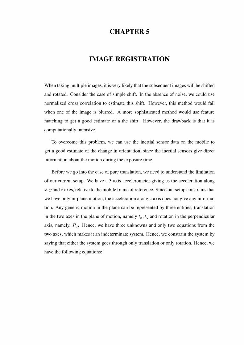
4.7 Actual blurred image. . . . . . . . . . . . . . . . . . . . . . . . . . 24
4.8 Deblurring using total blind method. . . . . . . . . . . . . . . . . . 24
4.9 Deblurring using our kernel as the initial estimate. . . . . . . . . . . 24
5.1 Example 1: Input image set . . . . . . . . . . . . . . . . . . . . . . 27
5.2 Example 1: Registered image pairs. . . . . . . . . . . . . . . . . . 27
5.3 Corresponding feature points calculated using SIFT based registrationby Vishwanath (2012–). The algorithm ran into error since not enoughpoints were found. . . . . . . . . . . . . . . . . . . . . . . . . . . 28
5.4 Example 2: Input image set . . . . . . . . . . . . . . . . . . . . . . 28
5.5 Example 2: Registered image pairs. . . . . . . . . . . . . . . . . . 28
5.6 Example 1: Input image set . . . . . . . . . . . . . . . . . . . . . . 30
v
5.7 Example 1: Registered images with very high blur and rotation. . . 30
5.8 Corresponding feature between the two images, calculated using SIFTbased image registration by Vishwanath (2012–). . . . . . . . . . . 30
5.9 Registed sharp image. Observe that the image is a little distorted alongthe horizontal axis. . . . . . . . . . . . . . . . . . . . . . . . . . . 30
5.10 Example 3: Input image set . . . . . . . . . . . . . . . . . . . . . . 31
5.11 Example 3: Registered images with very small blur and rotation. . . 31
6.1 Latent image and synthetic lurred image pair. . . . . . . . . . . . . 33
6.2 True depth map and estimated depth map. . . . . . . . . . . . . . . 33
6.3 Latent image and Blurred image pair. This is an example of close upshot. . . . . . . . . . . . . . . . . . . . . . . . . . . . . . . . . . . 34
6.4 Estimated depth map. Brighter area represents scene closer to the cam-era. . . . . . . . . . . . . . . . . . . . . . . . . . . . . . . . . . . 34
6.5 Latent image and Blurred image pair. Note that there is a misalignmentbetween the images. . . . . . . . . . . . . . . . . . . . . . . . . . . 34
6.6 Bad depth map. While the depth calculation at the edges is expected tobe accurate, the obtained depth map has erroneous edge values. . . . 34
6.7 First and last image of the 100 images. Note that in the first image, thescrew driver handle is in complete focus and in the last image, the bookis in complete focus. . . . . . . . . . . . . . . . . . . . . . . . . . 36
6.8 Estimated depth map. Objects nearer to the camera are darker. Observehow the objects have been segregated. . . . . . . . . . . . . . . . . 37
6.9 All focused image obtained using equation.6.5. . . . . . . . . . . . 37
vi
CHAPTER 1
INTRODUCTION
There has been a recent shift in computation from traditional computers to ubiquitous
mobile phones. With the ever increasing power of the mobiles, executing many of the
image processing algorithms on mobile has been made easy. Further, with the many
peripherals available for the mobile, such as the inertial sensors, controllable focus,
TCP and the bluetooth, computational photography is greatly advanced.
Photography using mobile has the innate problem of shake, which tends to blur the
images. Recovering the sharp image, given only the blurred image is a difficult task
due to the ill-posed nature of the problem. Any information about the motion during
the exposure time can help solve the problem with ease. Data from motion sensors
serves this purpose by providing the approximate trajectory of motion. Even when
taking multiple photographs which need to be aligned, like in the case of HDR images
from multiple normal exposure images, sensors data can be utilized to find the accurate
motion between the two shots.
A recent advancement in the field of computational photography is light field pho-
tography. Instead of a single focused image, multiple images are taken and various
regions of the image can be refocused. A mobile platform, which has the ability to
capture multiple images very fast with variable focus would pave way for research in
this area.
1.1 Goal of the project
We evaluate some of the important algorithms in computational photography by using
data obtained from the mobile. The aim is to prove that the extra information avail-
able from the motion sensors aides in increasing the efficiency of the image processing
algorithms.
The scope of the project extends to some of the consumer photography utilities. For
example, deblurring can be used to correcting images which have been degraded by
motion blur and would hence prevent a retake of the photo. Similarly, image registra-
tion can be used for stabilizing video when the camera is hand held. Further, this can
prove useful when the mobile device is fixed on top of a moving vehicle and we need a
stabilized video.
Throughout the project, we have assumed the availability of an accelerometer alone
as a motion sensor. While most part of the project has worked with data only from
accelerometer, we show that availability of other motion sensors like magnetometer
and gyroscope will make the algorithms more robust.
1.2 Prior work
The best known project involving the camera as an imaging device is the Camera 2.0
project by the Computer Science department at Stanford. The project involved hack-
ing the Nokia N900 firmware to write custom algorithms for focus. Further, the lab
also built a custom camera called Frankencamera which runs Linux and is completely
programmable, making it highly flexible.
While computational imaging on a mobile platform is relatively new, there has been
a lot of work on combining motion sensors with DSLR to perform accurate deblurring.
Joshi et al. (2010) Combines a 3 axis accelerometer and 3 axis gyroscope with a DSLR.
This paper is one of the main motivation for the image deblurring part. Bae et al.
(2013) builds upon Joshi et al. (2010) and explains how blind PSF estimation can be
combined with motion sensors data to improve deblurring. Šindelár and Šroubek (2013)
discusses the usage of a smart phone for deblurring images which have been degraded
by rotational blur. We try to use some of the ideas in this paper for deblurring for
translational blur.
Depth estimation, a well researched topic is of a lot of interest, especially in devices
for gaming like Kinect. A lot of literature exists on depth estimation using stereo vision.
A recent foray into this area is to estimate depth from a sharp and blurred image pair.
2
While most of the methods estimate it by estimating PSF from individual regions, not
much work has been done on fusing the image data with motion sensors data. We
present some of the methods for estimating depth using motion sensors data along with
sharp and blurred images.
Image registration exists for sharp images but not much literature exists on regis-
tering blurred images. Registration for symmetric blur has been discussed by Ojansivu
and Heikkila (2007), which is more applicable to the case of defocus blur. We deal with
a more non-symmetric case of motion blur and show that inertial sensors gives accurate
registration results.
1.3 Report layout
The project report is organized in the following manner. The chapter on Basic Theory
presents a brief account of the various algorithms and the mathematics involved in the
project. The chapter on The Device gives an in-depth account of the mobile platform,
the application written for the mobile platform and the host side software. The chapter
on Deblurring explains the implementation of the deblurring algorithm using the data
obtained from the mobile. Image Registration discusses about how inertial sensor data
can be used to reduce the search space of image registration process. Depth Estimation
has two parts, Depth estimation using motion blur and Depth estimation using focus
measure.
At the end of the report, we give a brief discussion about the future of the project
and how the algorithms can be taken forward. We concluded that though some of the
experiments were not successful, they gave very interesting results, which pave way for
future work.
3
CHAPTER 2
BASIC THEORY
We discuss the basics of some of the image processing algorithms in this chapter to gain
an understanding of the theory behind the project.
2.1 Position from Acceleration Data
A major part of the project involves estimating the trajectory of motion from accelerom-
eter data. In the current context, we assume that we have access to a three-axis ac-
celerometer alone. The three-axis accelerometer measures physical acceleration, which
is a combination of the acceleration due to gravity and any external force. Further,
the measured values are relative to the mobile frame of reference. Define ax, ay, az as
the acceleration due to external force, gx, gy, gz as the acceleration due to gravity from
the mobile’s frame of reference and ax, ay, az as the measured acceleration. Hence,
measured acceleration is modeled as
ax = gx + ax + nx (2.1)
ay = gy + ay + ny (2.2)
az = gz + az + nz, (2.3)
where nx, ny and nz are noise in measurements.For calculating the trajectory, we need
{ax, ay, az}. To obtain these values, we need to subtract the acceleration due to gravity.
However, we have no further information apart from the above equations. To get a good
estimate of the required acceleration, we assume that the gravity vector is quasi-static
when there is only translation in the mobile device. Hence, we estimate the gravity
vector as
gtx = αgt−1x + (1− α)atx (2.4)
gty = αgt−1y + (1− α)aty (2.5)
gtz = αgt−1z + (1− α)atz, (2.6)
where α is the LPF constant and lies between 0 and 1. Higher α gives rise to slower
variation in the gravity vector. We found empirically that 0.8 was a good value for the
constant.
Once we have the device acceleration, the equation for finding the trajectory of
motion would be
x(t) =
∫∫ t
0
ax(t)dt (2.7)
y(t) =
∫∫ t
0
ay(t)dt (2.8)
z(t) =
∫∫ t
0
az(t)dt. (2.9)
The discrete time approximation is
x[n] = (n∑t
n∑t
ax[n])×T 2 (2.10)
y[n] = (n∑t
n∑t
ay[n])×T 2 (2.11)
z[n] = (n∑t
n∑t
az[n])×T 2, (2.12)
where T is the sampling time of the motion sensors. Though this gives a good estimate
of the orientation of the device when there is no motion or the device acceleration when
there is only translation, the method suffers from two drawbacks:
1. The noise in measurement creates a random walk pattern. However, this mightnot be of major concern as it would only create a small disturbance in the over alltrajectory.
2. If the estimate of gravity vector is not correct, it would create a constant offset tothe device acceleration. This gives rise to drift, which will grow as t2, giving riseto wrong trajectory.
5
To understand drift, let us define a as the measured acceleration and a as theactual acceleration. Let the two quantities be related by the following equation:
a(t) = a(t) + ε, (2.13)
where ε is a small constant when compared to a(t). From the equation of thetrajectory, we get
x(t) =
∫∫a(t)dt (2.14)
=⇒ x(t) =
∫∫(a(t) + ε)dt (2.15)
=⇒ x(t) =
∫∫a(t)dt+
∫∫εdt (2.16)
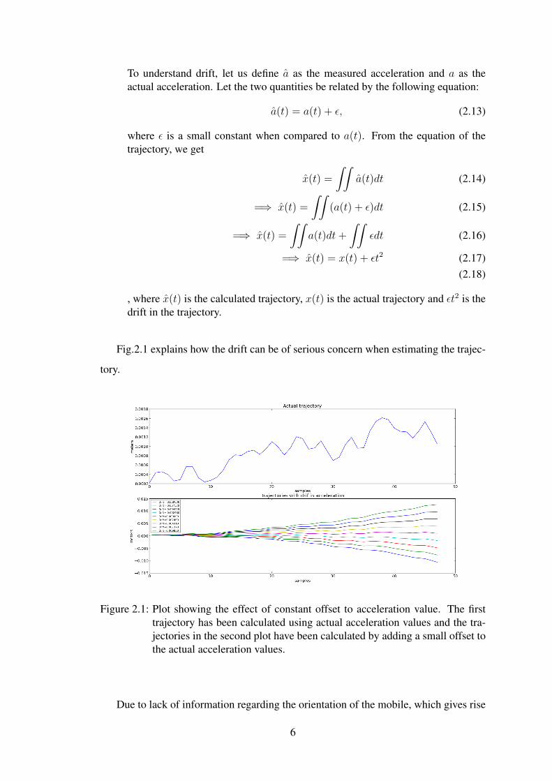
=⇒ x(t) = x(t) + εt2 (2.17)(2.18)
, where x(t) is the calculated trajectory, x(t) is the actual trajectory and εt2 is thedrift in the trajectory.
Fig.2.1 explains how the drift can be of serious concern when estimating the trajec-
tory.
Figure 2.1: Plot showing the effect of constant offset to acceleration value. The firsttrajectory has been calculated using actual acceleration values and the tra-jectories in the second plot have been calculated by adding a small offset tothe actual acceleration values.
Due to lack of information regarding the orientation of the mobile, which gives rise
6
to a bad estimate of gravity vector, the drift will exist and make the estimate unreliable.
In section 4, we will see the consequences of have a bad trajectory and possible ways
to rectify the problem.
2.2 Image blur
Image blur is equivalent to low pass filtering in 1D signals. While image blur is desired
in some applications like animation, it is undesirable when taking still photos. Two
types of blurs are of interest in this project, namely defocus blur and motion blur.
2.2.1 Defocus blur
Defocus blur is caused when the image of the object is not focussed on the sensor. This
arises only in real aperture cases when the focal length of the lens is finite and objects
are at varied distances.
The blur that arises due to defocus can be modeled as a 2D gaussian filtering oper-
ation. Hence, the point spread function is given by
h(x, y) =1
2πσ2e
−(x2+y2)
2σ2 , (2.19)
where σ depends on the depth of the object from the lens.
The defocus blur can be used in the shape from focus method, which varies one
particular parameter of the system like the lens position or the object position to bring
the object in focus. The idea is to have a focus measure. Pertuz et al. (2013) gives a
good outline of various focus measures used commonly. Further discussion about shape
from focus will be carried out in section 6.
2.2.2 Motion blur
Motion blur occurs due to relative motion between the scene and the camera during the
exposure time. The motion could either be the moving object or the motion induced
7
due to camera shake. This report deals with the problem of camera shake.
The process of camera shake can be considered as an averaging of multiple sharp
images shifted due to the camera motion. Hence for a planar scene,
ˆim(x, y) =1
N
N∑k
im(x− xk, y − yk) (2.20)
=⇒ ˆim(x, y) =1
N
N∑k
δ(xk, yk) ∗ im(x, y) (2.21)
where δ(xk, yk) is the Kronecker delta and ˆim is the observed image.
This can be rewritten as,
ˆim(x, y) = (1
N
N∑k
δ(xk, yk)) ∗ im(x, y) (2.22)
=⇒ ˆim(x, y) = h(x, y) ∗ im(x, y) (2.23)
h(x, y) is called the point spread function. If the image is not a planar scene, then
every point in the scene moves by a different amount due to the camera shake. If we
assume that there is no parallax error, we have,
ˆim(x, y) =∑t
δ(xt
d(x, y),
ytd(x, y)
) ∗ im(x, y) (2.24)
where d(x, y) is the depth of the image at (x, y). This space variant blurring operation
can be used to calculate depth information from the images, as objects at different
depths will be blurred to a different extent. Calculating d(x, y) gives the depth map
of the image.
2.3 Image deconvolution
The process of removing the blur in the image is known as image deconvolution. De-
convolution can be broadly of two types, blind and non- blind. If the PSF is known a
priori, it is known as non-blind deconvolution, else, it is known as blind deconvolution.
8
Blind deconvolution is an ill-posed problem, as an infinite combinations of latent image
and PSF can give rise to the observed image. Hence, various constraints are used when
trying to retrieve the latent imageFergus et al. (2006); Krishnan and Fergus (2009);
Levin et al. (2007a); Gupta et al. (2010).For example, an image can be considered as
piecewise smooth function with sharp images. Hence, we can try to reduce the total
variance of the obtained latent imageMoney and Kang (2006); Chan and Wong (1998).
If the blur is caused due to a straight line shaped PSF, analyzing the frequency domain
of the image can help retrieving the PSFOliveira et al. (2007).
On the other hand, non-blind deconvolution is less ill posed than the blind case,
as we have the PSF estimate. As discussed in the previous section, the blurred image
can be represented as the convolution of the PSF and the latent image in case of a
planar scene. This transforms into multiplication in the frequency domain. Hence, we
divide the image’s Fourier transform with the PSF’s Fourier transform to get the original
image. i.e
IMlatent(u, v) =ˆIM(u, v)
H(u, v), (2.25)
where H(u,v) is the DFT of the PSF h(x, y). However, the observed image is further
degraded by noise. Hence, the actual model of the observed image is
ˆim(x, y) = h(x, y) ∗ im(x, y) + n(x, y), (2.26)
where n(x, y) is the noise. The equation in the frequency domain can be loosely ex-
pressed as
ˆIM(u, v) = H(u, v).IM(u, v) +N(u, v) (2.27)
IMlatent(u, v) =ˆIM(u, v)
H(u, v)(2.28)
=⇒ IMlatent(u, v) = IM(u, v) +N(u, v)
H(u, v)(2.29)
Note that h(x, y) has a low frequency structure and noise has a high frequency structure.
Hence, the obtained image will have very high values in the high frequency region due
to the zeros of h(x, y) in the high frequency region.
9
Wiener deconvolution
Instead of simple division, we reformulate our problem as finding a filter which when
convolved with the observed image would return the latent image. Further, we wish
to reduce the error between the latent image and the image obtained by filtering the
observed image, i.e
min E|IM(u, v)− F. ˆIM(u, v)|2 (2.30)
ˆIM(u, v) = IM(u, v).H(u, v) +N(u, v), (2.31)
where E|.| is the expectation operator. Differentiating with respect to F , we get
F (u, v) =H∗(u, v)
|H(u, v)|2 + α(2.32)
=⇒ IMlatent(u, v) = ˆIM(u, v).F (u, v) (2.33)
=H∗(u, v). ˆIM(u, v)
|H(u, v)|2 + α(2.34)
where H∗(u, v) is the complex conjugate of H(u, v) and α is the inverse signal to noise
ratio of the image.
2.3.1 Regularized deconvolution
Since we know that the image blows up at the edges, we can impose a penalty on the
edge weights. Let gx and gy be the horizontal and vertical differentiation filters . Then,
we need
minimize |y − h ∗ x|2 + α|gx ∗ x|2 + α|gx ∗ x|2 (2.35)
=⇒ minimize |Y −HX|2 + α|GxX|2 + α|GxX|2 (2.36)
(2.37)
10
Where X represents the DFT of x. Differentiating the above equation with respect to
X , we get
X =H∗Y
|H|2 + α(G2x +G2
y)(2.38)
This is called regularized deconvolution. Apart from the simple deblurring algo-
rithms, there are other deconvolution methods, which work by reducing a certain cost
function. Literature on some of these can be found at Long and Brown; Wang et al.
(2009); Bioucas-Dias et al. (2006)
2.4 Image registration
Image registration finds application in many areas like medical imaging, aerial photog-
raphy and automated target recognition. In computational photography, image registra-
tion is used in wide number of areas like panorama stitching, depth estimation using
stereo vision and video stabilization.
Image registration involves finding the transform between a pair of images. The
transform could be a simple translation and rotation or a complicated warping. For
simple cases which involves only translation or only rotation, many of the frequency
based methods give good results. For advanced warping, feature based registration is
used. The SIFT based image registration, for example, identifies key points in each
image. Once we have the corresponding points in both the images, the problem is of
estimating the matrix that created this transform.
Note that when there is a large motion between the two images or one of the image
pairs is highly blurred, registration becomes difficult. Section 5 discusses about how
registration can be simplified using data from accelerometer. In this section, we will
look at a simple case of registering image pair which are transformed by shift alone.
11
2.4.1 Image registration using cross correlation
Let im1 and im2 be the image pairs. Since we are looking at a translation only model,
we have,
im2(x, y) = im1(x− x0, y − y0) (2.39)
Given these two images, we wish to estimate (x0, y0). A shift in the spacial domain
reflects as a phase multiplication in the frequency domain. Hence, if IM1 is the DFT of
im1, then,
IM2(u, v) = IM1(u, v)e−j(2πx0uM
+2πy0uN
) (2.40)
Let,
H(u, v) =IM1(u, v)×IM∗
2 (u, v)
|IM1(u, v)×IM2(u, v)|(2.41)
=⇒ H(u, v) = e−j(2πx0uM
+2πy0uN
) (2.42)
This gives,
h(x, y) = δ(x0, y0) (2.43)
Hence, the location of peak in h(x,y) will give the shift between the two images.
12
CHAPTER 3
THE DEVICE
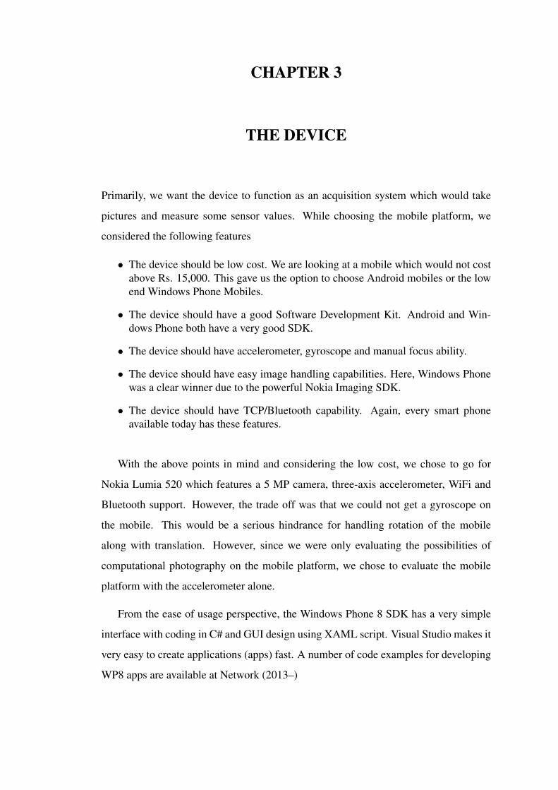
Primarily, we want the device to function as an acquisition system which would take
pictures and measure some sensor values. While choosing the mobile platform, we
considered the following features
• The device should be low cost. We are looking at a mobile which would not costabove Rs. 15,000. This gave us the option to choose Android mobiles or the lowend Windows Phone Mobiles.
• The device should have a good Software Development Kit. Android and Win-dows Phone both have a very good SDK.
• The device should have accelerometer, gyroscope and manual focus ability.
• The device should have easy image handling capabilities. Here, Windows Phonewas a clear winner due to the powerful Nokia Imaging SDK.
• The device should have TCP/Bluetooth capability. Again, every smart phoneavailable today has these features.
With the above points in mind and considering the low cost, we chose to go for
Nokia Lumia 520 which features a 5 MP camera, three-axis accelerometer, WiFi and
Bluetooth support. However, the trade off was that we could not get a gyroscope on
the mobile. This would be a serious hindrance for handling rotation of the mobile
along with translation. However, since we were only evaluating the possibilities of
computational photography on the mobile platform, we chose to evaluate the mobile
platform with the accelerometer alone.
From the ease of usage perspective, the Windows Phone 8 SDK has a very simple
interface with coding in C# and GUI design using XAML script. Visual Studio makes it
very easy to create applications (apps) fast. A number of code examples for developing
WP8 apps are available at Network (2013–)
3.1 Device side application
The app is mainly used for logging information to the computer so that algorithms can
be tested off line. The major advantage of this method is that it gives the power of the
computer along with the flexibility to experiment with different kinds of algorithms.
To make the application versatile and useful for future development, we added mul-
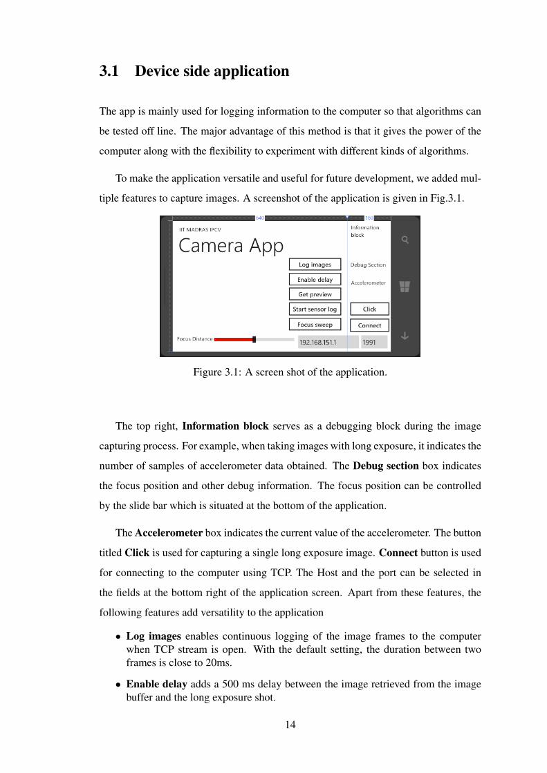
tiple features to capture images. A screenshot of the application is given in Fig.3.1.
Figure 3.1: A screen shot of the application.
The top right, Information block serves as a debugging block during the image
capturing process. For example, when taking images with long exposure, it indicates the
number of samples of accelerometer data obtained. The Debug section box indicates
the focus position and other debug information. The focus position can be controlled
by the slide bar which is situated at the bottom of the application.
The Accelerometer box indicates the current value of the accelerometer. The button
titled Click is used for capturing a single long exposure image. Connect button is used
for connecting to the computer using TCP. The Host and the port can be selected in
the fields at the bottom right of the application screen. Apart from these features, the
following features add versatility to the application
• Log images enables continuous logging of the image frames to the computerwhen TCP stream is open. With the default setting, the duration between twoframes is close to 20ms.
• Enable delay adds a 500 ms delay between the image retrieved from the imagebuffer and the long exposure shot.
14
• Enable preview captures an image from the image buffer (which can act as alatent image) prior to a long shot image.
• Start sensor log enables continous logging of the accelerometer data to the com-puter when the TCP stream is open.
• Focus sweep records 100 images with varied focus distance and sends them tothe computer.
The application has a 10ms timer, which takes care of all the logging and image
capture functions. While it is more apt to use a separate thread, we found that using a
timer was an easy method.
We discuss some of the methods implemented for logging the data and sending it
over TCP to understand the intricacies involved.
3.1.1 Logging accelerometer data during exposure
When the Click button is clicked, a camera capture sequence is started, which is pro-
grammed to take a picture with an exposure time of 200ms (adjustable). However, by
default, this suspends all other thread activities and is only released once the capture is
complete. This poses the problem that the accelerometer data cannot be logged during
this time, which is very important for estimating the blur kernel . To overcome this, we
use the async mode of camera capture(add ref to async camera capture website). In this
mode, the camera is initialized for capture and it returns to the thread. Meanwhile, a
busy flag is set and accelerometer data is recorded. When this is done, the busy flag is
unset, which stops the data logging. The code snippet is given below
public async void capture(bool get_preview, bool register){
// Get image previewif (get_preview == true){
_camera.GetPreviewBufferArgb(preview_image);}// Take a picture. Flag busy meanwhile.cam_busy = true;// If register mode is enabled, sleep for 500ms.if (register == true){
15
await System.Threading.Tasks.Task.Delay(500);}await _camsequence.StartCaptureAsync();cam_busy = false; // Done capture. Unset busy.transmit = true;imstream.Seek(0, SeekOrigin.Begin);
}
If an exposure time of 200ms is used, 20 accelerometer values are expected with a
10ms timer. However, close to 70 readings are obtained. This is due to the transfer time
of the image data also included in the capture time. To overcome this problem, a fast
moving image of a single point light source is taken. Frames of 20 samples out of 70
samples of the accelerometer data is used for estimating the best start and end times.
We use these start and end times for all the future kernel estimates.
3.1.2 Sending data over TCP
The TCP communication enables a communication stream between the mobile device
and the computer. With the stream open, it can be treated as a continuous information
channel, with no prior information about the size of the data being sent. To retrieve
data with this asynchronous type of data transmission, we encapsulate the data in key-
words which is known to the computer. This would boil down the problem to searching
for starting and ending keywords for each data type received. For example, if we are
sending a new image, we would use the keywords STIM and EDIM to encapsulate the
image data. An example:
// app_comsocket is the object representing the TCPconnection.
// app_comsocket.Send is used to send data over theconnection.
app_comsocket.Send("STIM\n"); // Start tokenapp_comsocket.Send(imdata); // Image dataapp_comsocket.Send("EDIM\n"); // End token
16
3.2 Host side application
Most of the host side application is written in Python. The reason for choosing python
is the vast support available for scientific computing, communication protocols, image
processing support and above all, python being free software. However, some of the
deblurring codes and super resolution are in MATLAB.
The communication from mobile to computer is done using the inbuilt socket mod-
ule in python. As mentioned in section 3.1.2, the data from the mobile is encapsulated
and sent in keywords. These keywords are used to parse the incoming data and split it
accordingly.
A number of functions have been written as part of host side software for data
reception, interpretation and image processing. Some of the main software modules are
discussed below.
3.2.1 TCP data handling
The TCP data handling, as the name suggests is responsible for receiving data from the
mobile, which includes images and motion sensors data. The main functions of this
module involve receiving sharp and blurred image pair, continuously receiving images
and continuously receiving motion sensor data. For example, in order to receive a sharp
and blurred image pair, we need to execute the function get_tcp_data(), which in
turn executes the following:
# Listen to the TCP socket and get data.dstring = tcp_listen();# Parse and save the data obtained from TCPsave_data(dstring);# Return a handle to the data, which consists of images and
the motion sensor data.return TCPDataHandle(dstring)
For continuous reception of images, we use the following function calls.
# All the images are encapsulated in tokens. Further, alltokens are
17
# Separated by the null character.strt_token = ’S\x00T\x00I\x00G\x00’end_token = ’E\x00D\x00I\x00G\x00’frame_token = ’S\x00T\x00I\x00M\x00’fstart = ’STIM’fend = ’EDIM’# First, receive the data from the mobile.continuous_recv(strt_token, end_token, frame_token,
’tmp/burst/tokens.dat’)# Once we have all the data, split it and save the first 100
images.extract_images(’tmp/burst/tokens.dat’, 100, fstart, fend,
’tmp/burst/src’)
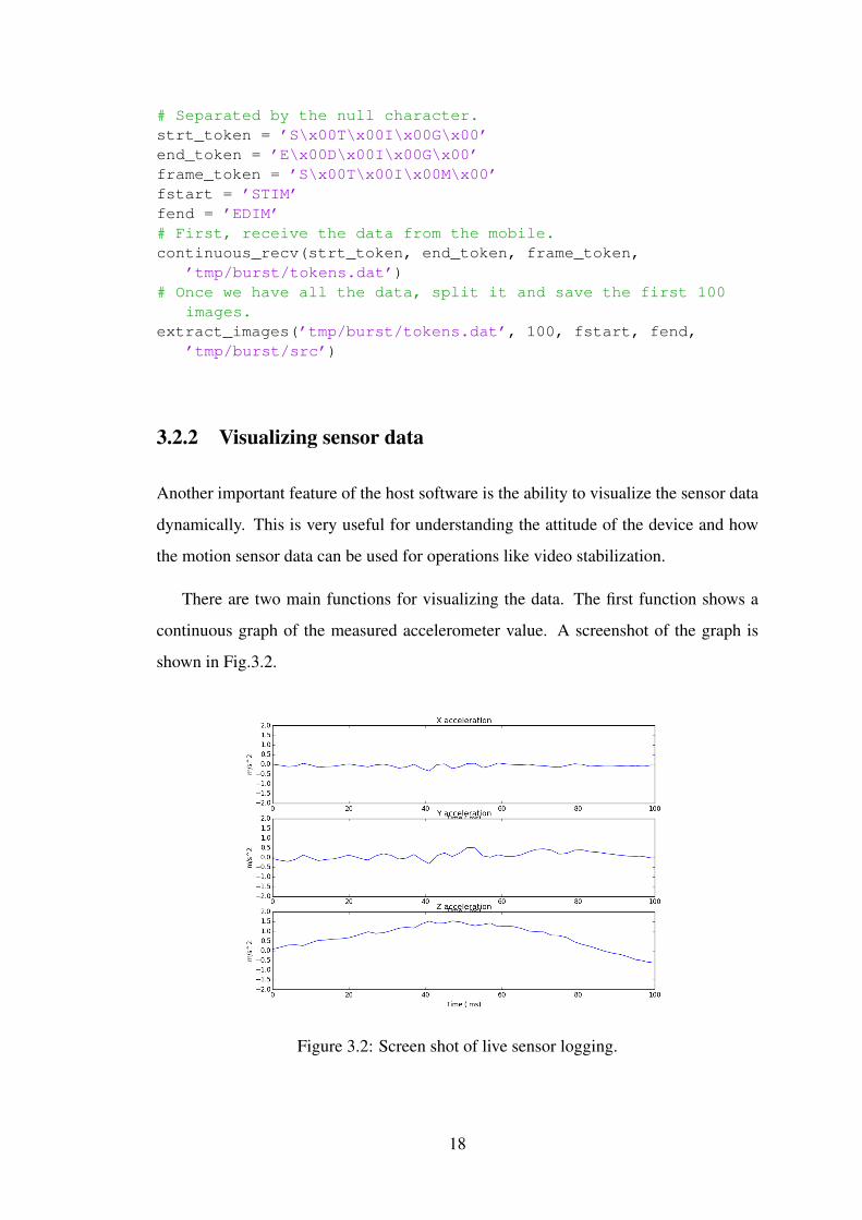
3.2.2 Visualizing sensor data
Another important feature of the host software is the ability to visualize the sensor data
dynamically. This is very useful for understanding the attitude of the device and how
the motion sensor data can be used for operations like video stabilization.
There are two main functions for visualizing the data. The first function shows a
continuous graph of the measured accelerometer value. A screenshot of the graph is
shown in Fig.3.2.
Figure 3.2: Screen shot of live sensor logging.
18
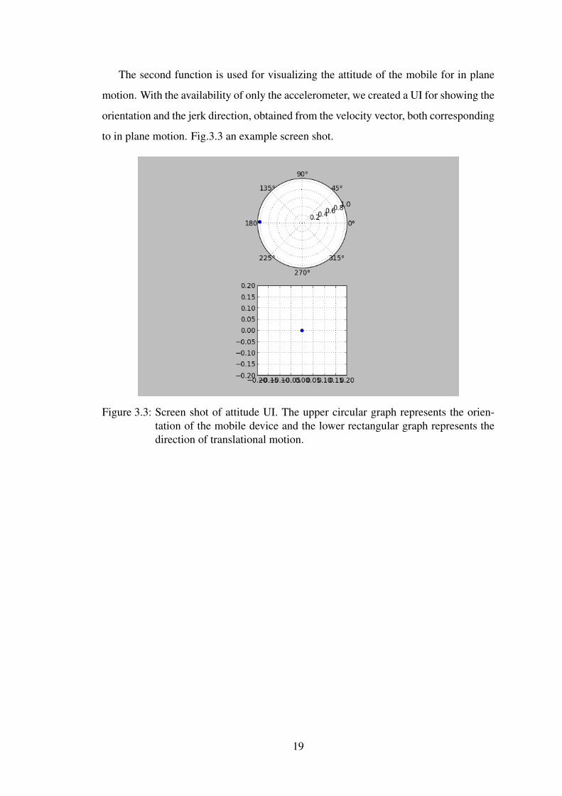
The second function is used for visualizing the attitude of the mobile for in plane
motion. With the availability of only the accelerometer, we created a UI for showing the
orientation and the jerk direction, obtained from the velocity vector, both corresponding
to in plane motion. Fig.3.3 an example screen shot.
Figure 3.3: Screen shot of attitude UI. The upper circular graph represents the orien-tation of the mobile device and the lower rectangular graph represents thedirection of translational motion.
19
CHAPTER 4
DEBLURRING
As mentioned in section 2.3, blurring due to motion is not desirable and we wish to
remove it. In this section, we will look at non blind and semi blind deconvolution
techniques.
Prior to deblurring, we need to estimate the blur kernel. As mentioned in 2.1, the
accelerometer data can be used to estimate the trajectory of the camera and thus the PSF
can be estimated. However, since we don’t know the scene depth and there is a drift
due to approximate value of gravity vector, we iterate through various possible depths
and shifts to find the appropriate image.
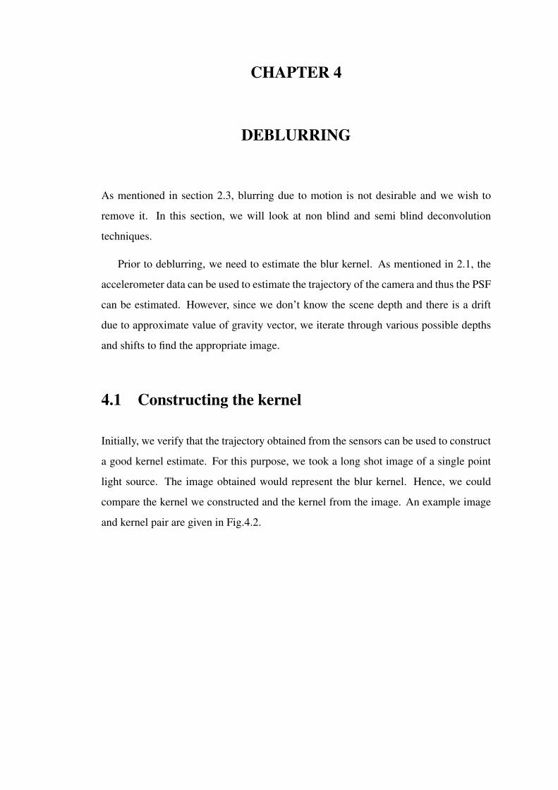
4.1 Constructing the kernel
Initially, we verify that the trajectory obtained from the sensors can be used to construct
a good kernel estimate. For this purpose, we took a long shot image of a single point
light source. The image obtained would represent the blur kernel. Hence, we could
compare the kernel we constructed and the kernel from the image. An example image
and kernel pair are given in Fig.4.2.
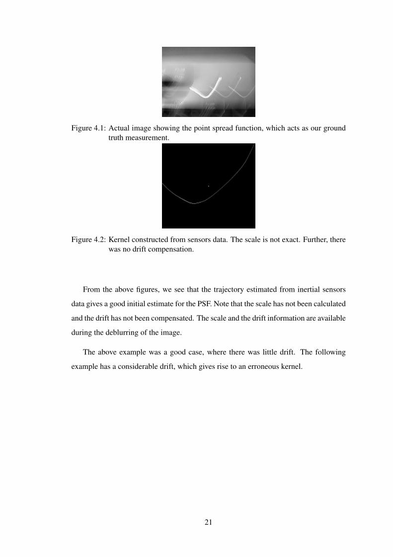
Figure 4.1: Actual image showing the point spread function, which acts as our groundtruth measurement.
Figure 4.2: Kernel constructed from sensors data. The scale is not exact. Further, therewas no drift compensation.
From the above figures, we see that the trajectory estimated from inertial sensors
data gives a good initial estimate for the PSF. Note that the scale has not been calculated
and the drift has not been compensated. The scale and the drift information are available
during the deblurring of the image.
The above example was a good case, where there was little drift. The following
example has a considerable drift, which gives rise to an erroneous kernel.
21
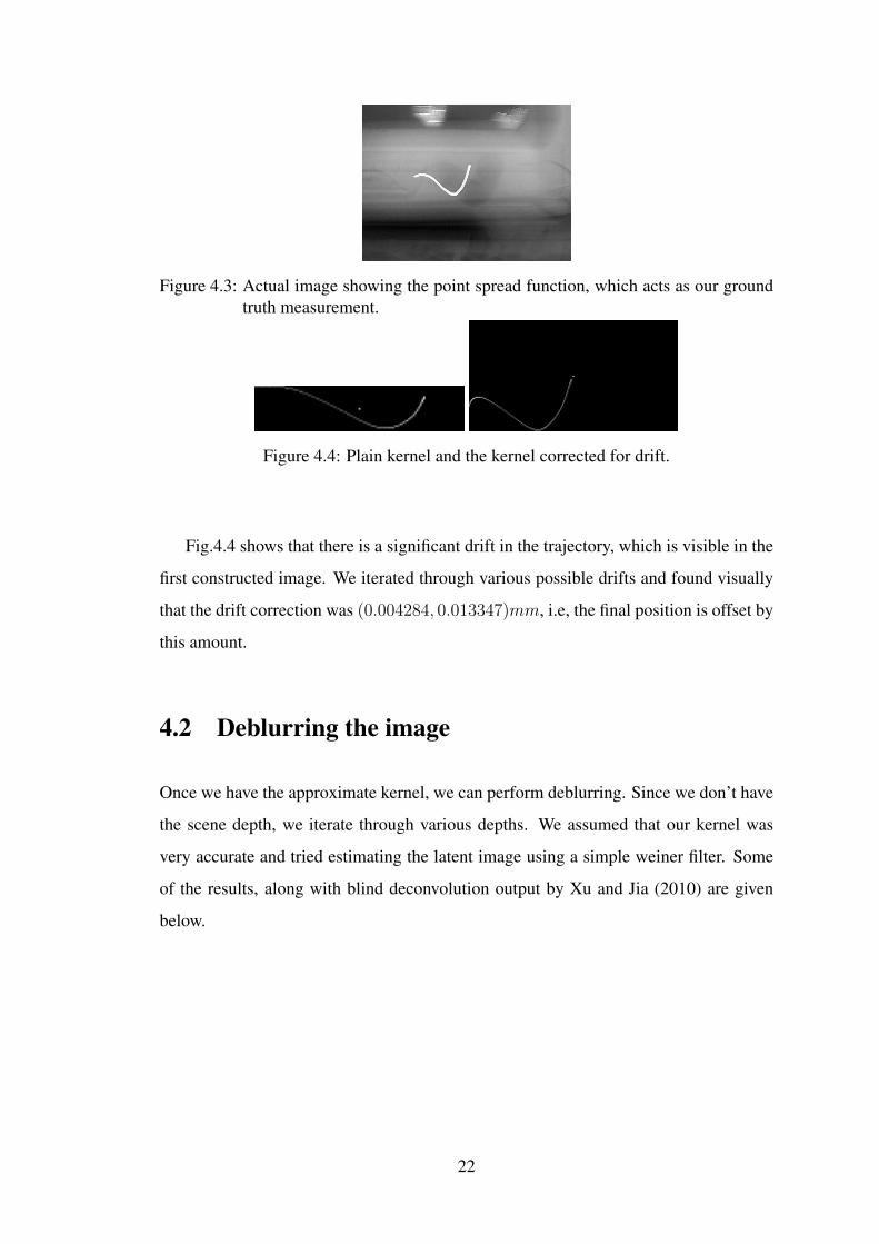
Figure 4.3: Actual image showing the point spread function, which acts as our groundtruth measurement.
Figure 4.4: Plain kernel and the kernel corrected for drift.
Fig.4.4 shows that there is a significant drift in the trajectory, which is visible in the
first constructed image. We iterated through various possible drifts and found visually
that the drift correction was (0.004284, 0.013347)mm, i.e, the final position is offset by
this amount.
4.2 Deblurring the image
Once we have the approximate kernel, we can perform deblurring. Since we don’t have
the scene depth, we iterate through various depths. We assumed that our kernel was
very accurate and tried estimating the latent image using a simple weiner filter. Some
of the results, along with blind deconvolution output by Xu and Jia (2010) are given
below.
22
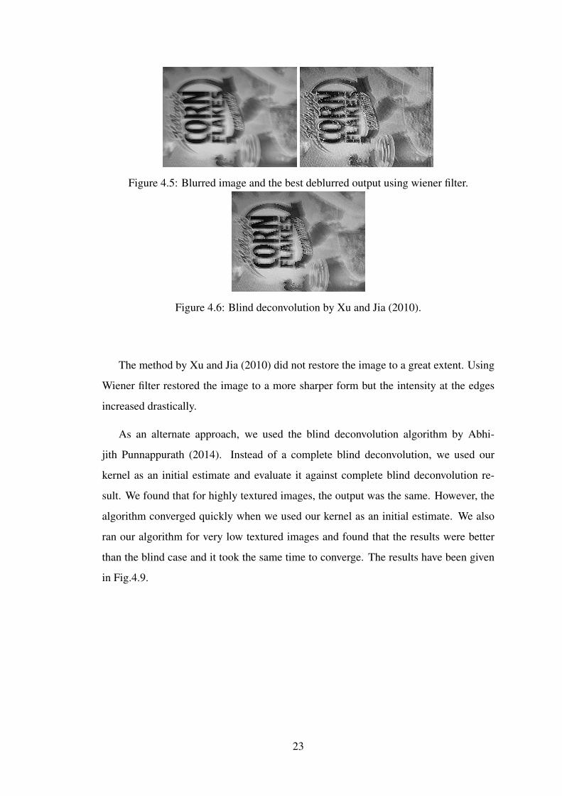
Figure 4.5: Blurred image and the best deblurred output using wiener filter.
Figure 4.6: Blind deconvolution by Xu and Jia (2010).
The method by Xu and Jia (2010) did not restore the image to a great extent. Using
Wiener filter restored the image to a more sharper form but the intensity at the edges
increased drastically.
As an alternate approach, we used the blind deconvolution algorithm by Abhi-
jith Punnappurath (2014). Instead of a complete blind deconvolution, we used our
kernel as an initial estimate and evaluate it against complete blind deconvolution re-
sult. We found that for highly textured images, the output was the same. However, the
algorithm converged quickly when we used our kernel as an initial estimate. We also
ran our algorithm for very low textured images and found that the results were better
than the blind case and it took the same time to converge. The results have been given
in Fig.4.9.
23
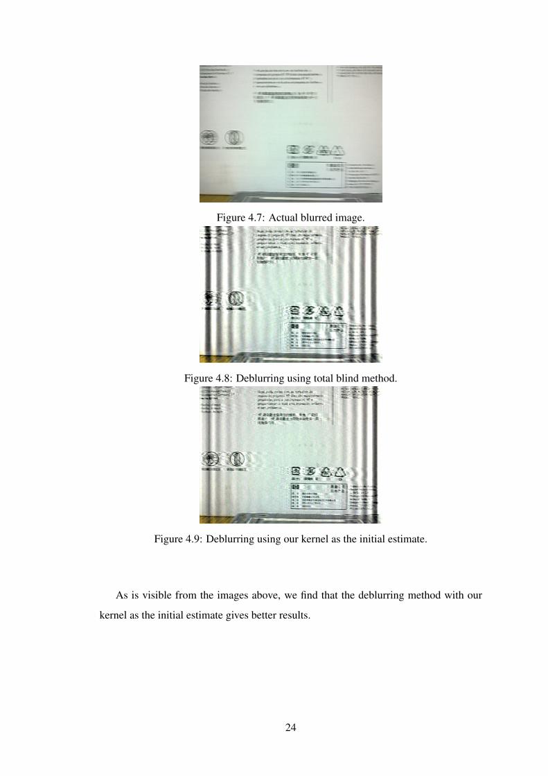
Figure 4.7: Actual blurred image.
Figure 4.8: Deblurring using total blind method.
Figure 4.9: Deblurring using our kernel as the initial estimate.
As is visible from the images above, we find that the deblurring method with our
kernel as the initial estimate gives better results.
24
CHAPTER 5
IMAGE REGISTRATION
When taking multiple images, it is very likely that the subsequent images will be shifted
and rotated. Consider the case of simple shift. In the absence of noise, we could use
normalized cross correlation to estimate this shift. However, this method would fail
when one of the image is blurred. A more sophisticated method would use feature
matching to get a good estimate of a the shift. However, the drawback is that it is
computationally intensive.
To overcome this problem, we can use the inertial sensor data on the mobile to
get a good estimate of the change in orientation, since the inertial sensors give direct
information about the motion during the exposure time.
Before we go into the case of pure translation, we need to understand the limitation
of our current setup. We have a 3-axis accelerometer giving us the acceleration along
x, y and z axes, relative to the mobile frame of reference. Since our setup constrains that
we have only in-plane motion, the acceleration along z axis does not give any informa-
tion. Any generic motion in the plane can be represented by three entities, translation
in the two axes in the plane of motion, namely tx, ty and rotation in the perpendicular
axis, namely, Rz. Hence, we have three unknowns and only two equations from the
two axes, which makes it an indeterminate system. Hence, we constrain the system by
saying that either the system goes through only translation or only rotation. Hence, we
have the following equations:
txi =
∫∫axdt (5.1)
tyi =
∫∫aydt (5.2)
or (5.3)
θi = tan−1(ay/ax) (5.4)
(5.5)
We look at two cases, one of pure translation and another of pure rotation.
5.1 Pure translation
As mentioned in 3.1.1, we can determine the trajectory of the device from the ac-
celerometer data, which is given by
xfinal =
∫ tfinal
tinit
∫ tfinal
tinit
axdt (5.6)
yfinal =
∫ tfinal
tinit
∫ tfinal
tinit
aydt. (5.7)
We wish to find the shifts xshift, yshift such that the RMS difference between the first
image and the shifted second image is reduced. i.e
min ||im1(x, y)− im2(x− xshift, y − yshift)||2 (5.8)
The calculated final position is in mm and needs to be converted into pixel dimension.
However, we don’t have the distance of the scene from the camera, which makes it an
ill-posed problem. To overcome this, we iterate through various scales and find out the
correct scale using RMS error. Hence,
(xshift, yshift) = argmink{∑x
∑y
(im1(x, y)− im2(x− k ∗ xfinal, y − k ∗ yfinal))2}
(5.9)
26
Note that the maximum shift is bound due to the finite duration. Hence, our search
space is drastically reduced from 360o in the blind case to a small sector(it is not a
straight line due to the drift associated with the accelerometer readings) with the help
of accelerometer data.
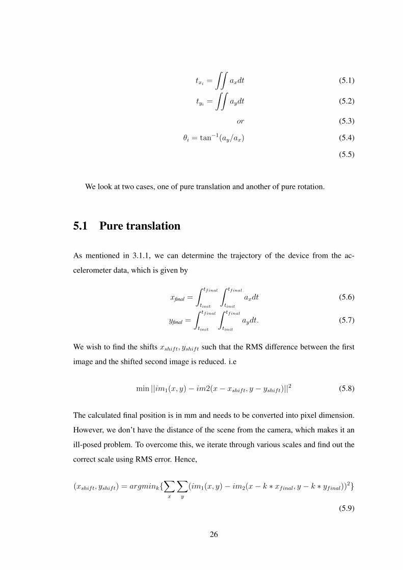
Fig.5.5 shows example outputs of the algorithm.
Figure 5.1: Example 1: Input image set
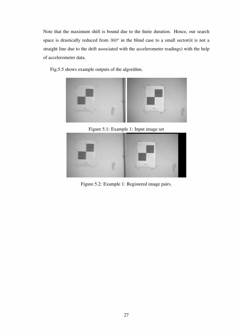
Figure 5.2: Example 1: Registered image pairs.
27
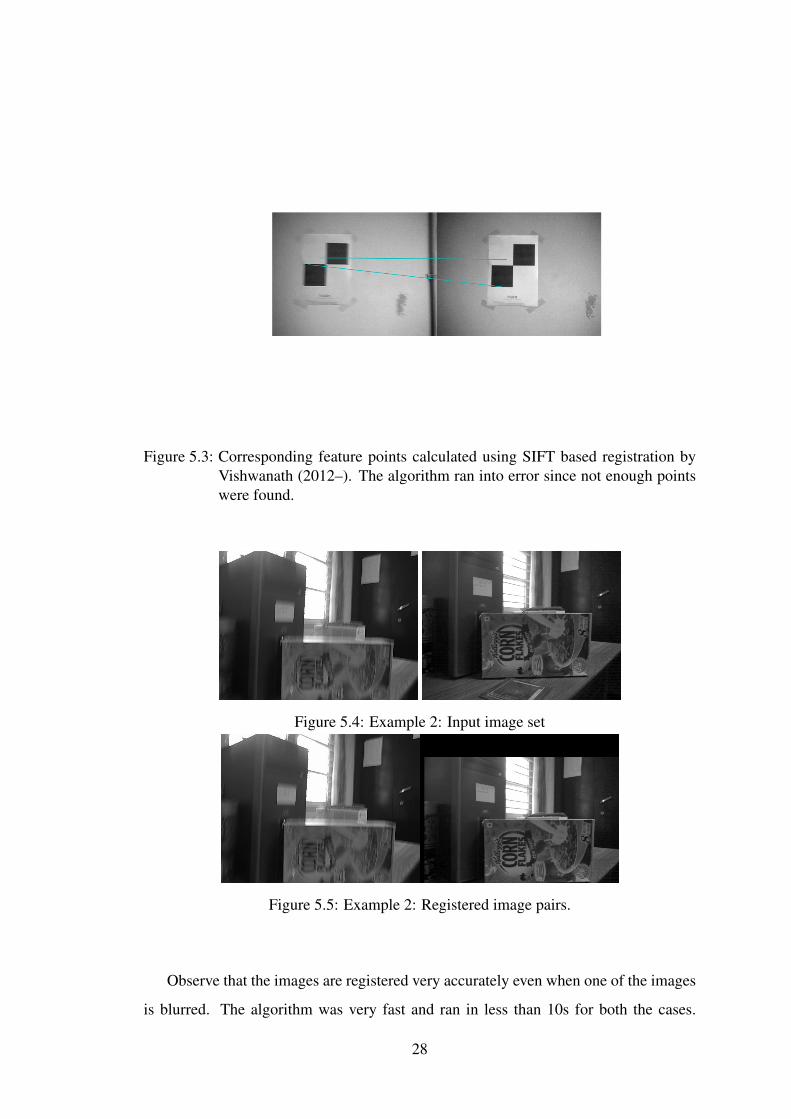
Figure 5.3: Corresponding feature points calculated using SIFT based registration byVishwanath (2012–). The algorithm ran into error since not enough pointswere found.
Figure 5.4: Example 2: Input image set
Figure 5.5: Example 2: Registered image pairs.
Observe that the images are registered very accurately even when one of the images
is blurred. The algorithm was very fast and ran in less than 10s for both the cases.
28
Further, as we have a good estimate of the direction of motion, finer registration can
be done by increasing the search space, after performing coarse registration using the
above mentioned method. On the other hand, the SIFT based image registration ran
into error due to very less matching feature points.
5.2 Pure rotation
Assuming only in-plane rotation, we can relate the measured acceleration to world ac-
celeration (in the absence of other forces) as
ax = g cos θ (5.10)
ay = g sin θ (5.11)
Where θ is the orientation of the device. Hence, the orientation of the mobile can be
estimated as
θ = tan−1(ayax
) (5.12)
As in the pure translation case, we take two images, one non-blurred and another
blurred, both separated by 500ms duration. We only rotate the device during this du-
ration. Hence, we can use the acceleration values estimated during this time frame to
correct for the rotation. Note that the process of rotation will also induce a small trans-
lation in the image. This makes the RMS error method of finding the appropriate angle
difficult. We hence use normalized cross correlation, which is independent of the shift.
Thus,
θ = argmaxt{F−1
(F(im1).F(R(im2, θt))
∗
|F(im1).F(R(im2, θt))|
)} (5.13)
Where F(.) is the 2D discrete Fourier transform, F−1(.) is the 2D discrete inverse
Fourier transform andR(im, θ) rotates the image by θ degrees.
Fig.5.11 gives three examples of registration using the proposed method.
29
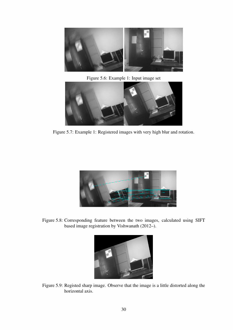
Figure 5.6: Example 1: Input image set
Figure 5.7: Example 1: Registered images with very high blur and rotation.
Figure 5.8: Corresponding feature between the two images, calculated using SIFTbased image registration by Vishwanath (2012–).
Figure 5.9: Registed sharp image. Observe that the image is a little distorted along thehorizontal axis.
30
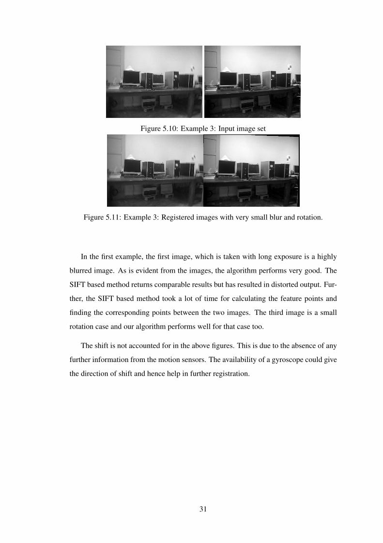
Figure 5.10: Example 3: Input image set
Figure 5.11: Example 3: Registered images with very small blur and rotation.
In the first example, the first image, which is taken with long exposure is a highly
blurred image. As is evident from the images, the algorithm performs very good. The
SIFT based method returns comparable results but has resulted in distorted output. Fur-
ther, the SIFT based method took a lot of time for calculating the feature points and
finding the corresponding points between the two images. The third image is a small
rotation case and our algorithm performs well for that case too.
The shift is not accounted for in the above figures. This is due to the absence of any
further information from the motion sensors. The availability of a gyroscope could give
the direction of shift and hence help in further registration.
31
CHAPTER 6
DEPTH ESTIMATION
When taking an image, due to the variable depth of the scene, the amount of blur in-
duced at every pixel due to defocus or motion of the camera is different. We use this
information to estimate the depth from images using two methods, namely depth from
motion blur and depth from focus.
6.1 Depth from motion blur
Section 2.2.2 gives a brief discussion about how every point in the image gets blurred
by a different blur kernel due to the depth profile. If we neglect the parallax error,
we can see that the only variation in the blur kernel is the scale. Hence, estimating
the depth profile boils down to estimating the scale of the blur kernel at different points.
Estimating depth from a blurred and latent image has been discussed in Paramanand and
Rajagopalan (2010). However, the method requires estimation of depth at every point,
due to the absence of any motion information. Levin et al. (2007b) uses coded aperture
for extracting the depth profile from the image. However, the paper has good discussion
about estimating depth from two images, which is more apt for our discussion.
In the experimental setup, we capture two images, one with very short exposure
and another with long exposure. Further, along with the two images, the motion of
the camera is estimated by logging the accelerometer values. Thus, we have the latent
image, the blurred image and the blur kernel. We need to estimate the scale of the blur
kernel at each point. Prior to estimating the depth, it is very important that the two
images are aligned. We would show that misalignment could be a major reason for
wrong depth profiles. However, for small shifts, we found that iterating through a small
space to search for the right shifts was enough.
To estimate the depth at each point, we iterate through various blur kernel sizes and
calculate the difference between the blurred image and the blurred latent image for each
scale of the kernel. If the scale is correct at a given position, the error at that point will
be the least and that would be assigned as the depth value. Hence, we can formulate our
algorithm as
k(x, y) = argmind{|im(x, y)blurred − h(x, y, d) ∗ imlatent(x, y)|2} (6.1)
Where h(x, y, d) is the kernel with scale value of d. While this works for the ideal case,
the real depth map is very noisy. Hence, we low pass filter the error map with a box
filter. This algorithm works very well when there is good texture in the image. Further,
it is necessary that the kernel is very accurate, else the depth map will go wrong.
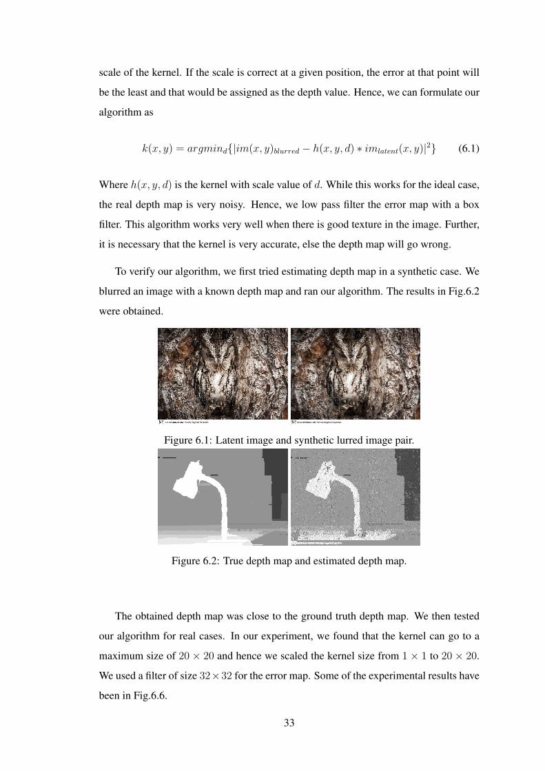
To verify our algorithm, we first tried estimating depth map in a synthetic case. We
blurred an image with a known depth map and ran our algorithm. The results in Fig.6.2
were obtained.
Figure 6.1: Latent image and synthetic lurred image pair.
Figure 6.2: True depth map and estimated depth map.
The obtained depth map was close to the ground truth depth map. We then tested
our algorithm for real cases. In our experiment, we found that the kernel can go to a
maximum size of 20 × 20 and hence we scaled the kernel size from 1 × 1 to 20 × 20.
We used a filter of size 32×32 for the error map. Some of the experimental results have
been in Fig.6.6.
33
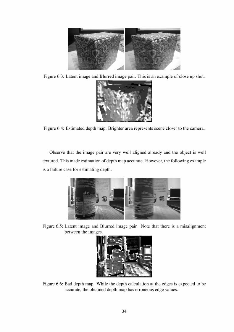
Figure 6.3: Latent image and Blurred image pair. This is an example of close up shot.
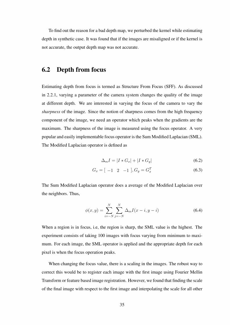
Figure 6.4: Estimated depth map. Brighter area represents scene closer to the camera.
Observe that the image pair are very well aligned already and the object is well
textured. This made estimation of depth map accurate. However, the following example
is a failure case for estimating depth.
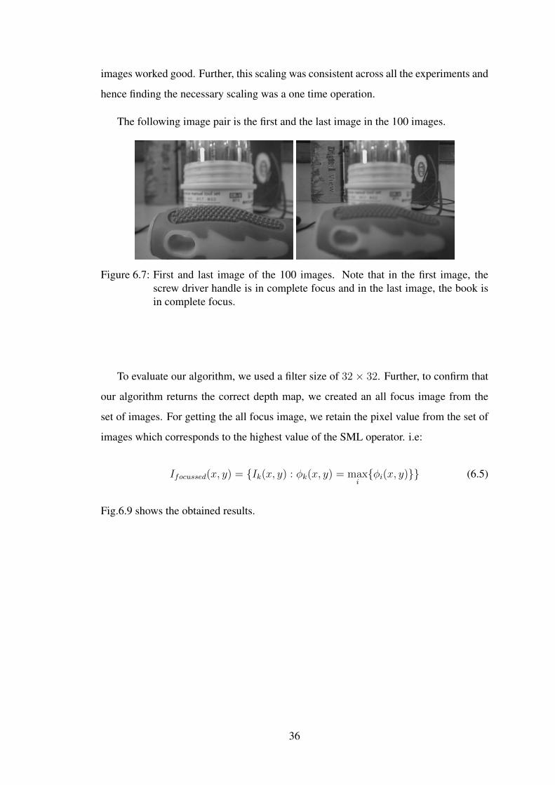
Figure 6.5: Latent image and Blurred image pair. Note that there is a misalignmentbetween the images.
Figure 6.6: Bad depth map. While the depth calculation at the edges is expected to beaccurate, the obtained depth map has erroneous edge values.
34
To find out the reason for a bad depth map, we perturbed the kernel while estimating
depth in synthetic case. It was found that if the images are misaligned or if the kernel is
not accurate, the output depth map was not accurate.
6.2 Depth from focus
Estimating depth from focus is termed as Structure From Focus (SFF). As discussed
in 2.2.1, varying a parameter of the camera system changes the quality of the image
at different depth. We are interested in varying the focus of the camera to vary the
sharpness of the image. Since the notion of sharpness comes from the high frequency
component of the image, we need an operator which peaks when the gradients are the
maximum. The sharpness of the image is measured using the focus operator. A very
popular and easily implementable focus operator is the Sum Modified Laplacian (SML).
The Modified Laplacian operator is defined as
∆mI = |I ∗Gx|+ |I ∗Gy| (6.2)
Gx = [ −1 2 −1 ], Gy = GTx (6.3)
The Sum Modified Laplacian operator does a average of the Modified Laplacian over
the neighbors. Thus,
φ(x, y) =N∑
i=−N
N∑j=−N
∆mI(x− i, y − i) (6.4)
When a region is in focus, i.e, the region is sharp, the SML value is the highest. The
experiment consists of taking 100 images with focus varying from minimum to maxi-
mum. For each image, the SML operator is applied and the appropriate depth for each
pixel is when the focus operation peaks.
When changing the focus value, there is a scaling in the images. The robust way to
correct this would be to register each image with the first image using Fourier Mellin
Transform or feature based image registration. However, we found that finding the scale
of the final image with respect to the first image and interpolating the scale for all other
35
images worked good. Further, this scaling was consistent across all the experiments and
hence finding the necessary scaling was a one time operation.
The following image pair is the first and the last image in the 100 images.
Figure 6.7: First and last image of the 100 images. Note that in the first image, thescrew driver handle is in complete focus and in the last image, the book isin complete focus.
To evaluate our algorithm, we used a filter size of 32× 32. Further, to confirm that
our algorithm returns the correct depth map, we created an all focus image from the
set of images. For getting the all focus image, we retain the pixel value from the set of
images which corresponds to the highest value of the SML operator. i.e:
Ifocussed(x, y) = {Ik(x, y) : φk(x, y) = maxi{φi(x, y)}} (6.5)
Fig.6.9 shows the obtained results.
36
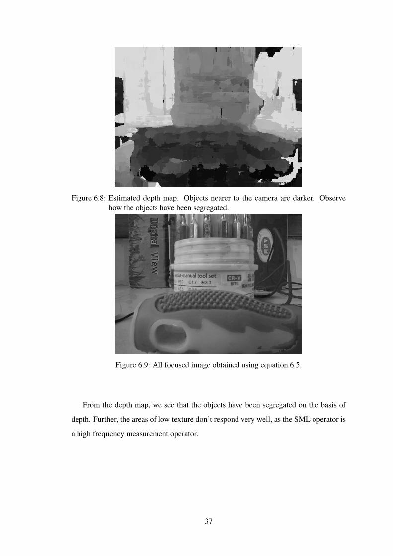
Figure 6.8: Estimated depth map. Objects nearer to the camera are darker. Observehow the objects have been segregated.
Figure 6.9: All focused image obtained using equation.6.5.
From the depth map, we see that the objects have been segregated on the basis of
depth. Further, the areas of low texture don’t respond very well, as the SML operator is
a high frequency measurement operator.
37
CHAPTER 7
CONCLUSION
We have evaluated some of the important image restoration and registration algorithm
with data from a mobile. Some of the results are very promising, while some of them
weren’t very good. In particular, estimating depth from focus, and image registration
have given very good results. Depth estimation from blurred and latent image pair was
good to a certain extent but was very sensitive to the accuracy of the kernel estimate.
The results can be made better with the presence of a magnetometer, which would pro-
vide accurate orientation information, thus making the estimate of trajectory of motion
more accurate. The image deblurring, while proving interesting results like fast conver-
gence and better results in case of low texture images, has good scope for improvement.
While all the codes were run offline for ease of research purpose, we saw that the
algorithms were very simple and efficient due to availability of information from motion
sensors. Hence, porting these algorithms onto a mobile should be an easy task.
7.1 Future work
Along with the evaluation of major algorithms for registration and restoration, the
project has provided a good stage for future development. All the discussed algorithms
can be immediately ported to a mobile platform with great ease, which would provide
a very powerful computational imaging device.
Along from the usefulness of our algorithms, the mobile application is a very ver-
satile one and would serve well for future experiments with different algorithms. With
features like continuous logging of images, continuous logging of motion sensor data,
capturing low exposure noisy image and long exposure blurred image and freely chang-
ing parameters of the camera, the device would prove very useful for working on com-
putational imaging on a mobile platform.
Apart from the sunny side of the project, there were some parts which were not
addressed appropriately. Not much effort was put into writing a more efficient semi-
blind deconvolution algorithm. However, this was partly not possible due to absence
of magnetometer on our device. Further, the mobile currently does all the job using a
10ms timer, which might be inefficient. Unloading the work onto a separate thread will
not only make it neat, but it would make it much more efficient.
We also started working on multi-frame super-resolution but were not able to go
further due to time constraints. As registration forms a major part of super-resolution,
the data from the inertial sensors can greatly aide in reducing the complexity of this
step.
We are looking forward to open our code to public so that people who are interested
can contribute. The code will be the property of the lab and the author of the report
would like to credit all the work to the lab.
39
REFERENCES
Abhijith Punnappurath, G. S., A. N. Rajagopalan, Blind restoration of aerial im-agery degraded by spatially varying motion blur. In Society of Photographic Instru-mentation Engineers, 2014. Proceedings SPIE’14. 2014.
Bae, H., C. C. Fowlkes, and P. H. Chou, Accurate motion deblurring using cameramotion tracking and scene depth. In WACV . 2013.
Bioucas-Dias, J. M., M. A. Figueiredo, and J. P. Oliveira, Total variation-based im-age deconvolution: a majorization-minimization approach. In Acoustics, Speech andSignal Processing, 2006. ICASSP 2006 Proceedings. 2006 IEEE International Con-ference on, volume 2. IEEE, 2006.
Chan, T. F. and C.-K. Wong (1998). Total variation blind deconvolution. Image Pro-cessing, IEEE Transactions on, 7(3), 370–375.
Fergus, R., B. Singh, A. Hertzmann, S. T. Roweis, and W. T. Freeman, Removingcamera shake from a single photograph. In ACM Transactions on Graphics (TOG),volume 25. ACM, 2006.
Freeman, W. T. and E. H. Adelson (1991). The design and use of steerable filters.IEEE Transactions on Pattern analysis and machine intelligence, 13(9), 891–906.
Gupta, A., N. Joshi, C. L. Zitnick, M. Cohen, and B. Curless, Single image de-blurring using motion density functions. In Computer Vision–ECCV 2010. Springer,2010, 171–184.
Jin, H. and P. Favaro, A variational approach to shape from defocus. In ComputerVisionâATECCV 2002. Springer, 2002, 18–30.
Joshi, N., S. B. Kang, C. L. Zitnick, and R. Szeliski (2010). Image deblurring usinginertial measurement sensors. ACM Transactions on Graphics (TOG), 29(4), 30.
Jung, S.-H. and C. J. Taylor, Camera trajectory estimation using inertial sensor mea-surements and structure from motion results. In Computer Vision and Pattern Recog-nition, 2001. CVPR 2001. Proceedings of the 2001 IEEE Computer Society Confer-ence on, volume 2. IEEE, 2001.
Krishnan, D. and R. Fergus, Fast image deconvolution using hyper-laplacian priors.In NIPS, volume 22. 2009.
Levin, A., R. Fergus, F. Durand, and W. T. Freeman (2007a). Deconvolution usingnatural image priors. ACM Transactions on Graphics (TOG), 26(3), 0–2.
Levin, A., R. Fergus, F. Durand, and W. T. Freeman (2007b). Image and depth froma conventional camera with a coded aperture. ACM Transactions on Graphics (TOG),26(3), 70.
40
Long, Y.-W. T. P. T. and G. M. S. Brown (). Richardson-lucy deblurring for scenesunder projective motion path.
Losch, S. (2009). Depth from Blur: Combining Image Deblurring and Depth Esti-mation. Ph.D. thesis, Department of Computer Science, Saarland University, Saar-brÃijcken, Germany.
Money, J. H. and S. H. Kang (2006). Total variation semi-blind deconvolution usingshock filters. submitted to Image and Vision Computing.
Network, M. D. (2013–). Windows phone samples: learn through code. URL http://code.msdn.microsoft.com/wpapps/.
Ojansivu, V. and J. Heikkila (2007). Image registration using blur-invariant phasecorrelation. Signal Processing Letters, IEEE, 14(7), 449–452.
Oliveira, J. P., M. A. Figueiredo, and J. M. Bioucas-Dias, Blind estimation of motionblur parameters for image deconvolution. In Pattern Recognition and Image Analysis.Springer, 2007, 604–611.
Paramanand, C. and A. Rajagopalan, Unscented transformation for depth frommotion-blur in videos. In Computer Vision and Pattern Recognition Workshops(CVPRW), 2010 IEEE Computer Society Conference on. IEEE, 2010.
Pertuz, S., D. Puig, and M. A. Garcia (2013). Analysis of focus measure operators forshape-from-focus. Pattern Recognition, 46(5), 1415–1432.
Portilla, J. and R. Navarro, Efficient method for space-variant low-pass filtering. In VIINational Symposium on Pattern Recognition and Image Analysis, volume 1. 1997.
Reddy, D., J. Bai, and R. Ramamoorthi (). External mask based depth and light fieldcamera.
Šindelár, O. and F. Šroubek (2013). Image deblurring in smartphone devices usingbuilt-in inertial measurement sensors. Journal of Electronic Imaging, 22(1), 011003–011003.
Sroubek, F. and P. Milanfar (2012). Robust multichannel blind deconvolution via fastalternating minimization. Image Processing, IEEE Transactions on, 21(4), 1687–1700.
Subbarao, M. and N. Gurumoorthy, Depth recovery from blurred edges. In Com-puter Vision and Pattern Recognition, 1988. Proceedings CVPR’88., Computer Soci-ety Conference on. IEEE, 1988.
Vandewalle, P. (2006). Super-resolution from unregistered aliased images. Ph.D. the-sis, Ecole Polytechnique Fédérale de Lausanne.
Vishwanath, S. R. V. (2012–). Simple image registration using sift and ransac algo-rithm. URL https://github.com/vishwa91/pyimreg.
41

Wang, C., L. Sun, Z. Chen, S. Yang, and J. Zhang, Robust inter-scale non-blindimage motion deblurring. In Image Processing (ICIP), 2009 16th IEEE InternationalConference on. IEEE, 2009.
Xiao, F., A. Silverstein, and J. Farrell, Camera-motion and effective spatial resolution.In International Congress of Imaging Science, Rochester, NY . 2006.
Xiong, Y. and S. A. Shafer, Depth from focusing and defocusing. In Computer Vi-sion and Pattern Recognition, 1993. Proceedings CVPR’93., 1993 IEEE ComputerSociety Conference on. IEEE, 1993.
Xu, L. and J. Jia, Two-phase kernel estimation for robust motion deblurring. In Com-puter Vision–ECCV 2010. Springer, 2010, 157–170.
42