Understanding City Traffic Dynamics Utilizing Sensor and Textual Observations

Pramod Anantharam, Krishnaprasad Thirunarayan, Surendra Marupudi, Amit Sheth, and Tanvi BanerjeeKno.e.sis, Wright State University, Dayton OH, USA{pramod,tkprasad,surendra,amit,tanvi}@knoesis.org

Abstract

Understanding speed and travel-time dynamics in re-sponse to various city related events is an important andchallenging problem. Sensor data (numerical) contain-ing average speed of vehicles passing through a roadlink can be interpreted in terms of traffic related inci-dent reports from city authorities and social media data(textual), providing a complementary understanding oftraffic dynamics. State-of-the-art research is focused oneither analyzing sensor observations or citizen observa-tions; we seek to exploit both in a synergistic manner.We demonstrate the role of domain knowledge in cap-turing the non-linearity of speed and travel-time dynam-ics by segmenting speed and travel-time observationsinto simpler components amenable to description us-ing linear models such as Linear Dynamical System(LDS). Specifically, we propose Restricted SwitchingLinear Dynamical System (RSLDS) to model normalspeed and travel time dynamics and thereby charac-terize anomalous dynamics. We utilize the city trafficevents extracted from text to explain anomalous dynam-ics. We present a large scale evaluation of the proposedapproach on a real-world traffic and twitter dataset col-lected over a year with promising results.

IntroductionThere is an increasing body of research on understandingtraffic flow for efficient management of mobility in a city.Currently, there are over 1 billion cars on roads and thisnumber is expected to double by 2020 (IBM 2014). Vehic-ular traffic increased by 236% from 1981 to 2001 while theworld population grew only by 20% (IBM 2014). Increasedurbanization has impacted the mobility of people in cities.Zero traffic fatalities and minimizing traffic delays are someof the grand challenges in Cyber-Physical Systems (Rajku-mar et al. 2010). To overcome these challenges, we needa deeper understanding of the interactions between variousevents in a city and its impact on traffic. Current traffic as-sessment techniques focus on analysis of fine grained sen-sor observations to predict delays (Ko and Guensler 2005;Anderson and Bell 1997; De Fabritiis, Ragona, and Valenti2008; Sun, Zhang, and Yu 2006). However, these are lim-

Copyright c© 2016, Association for the Advancement of ArtificialIntelligence (www.aaai.org). All rights reserved.

ited and opaque, and do not explain the reasons for traf-fic flow variations. Increasingly, observations of real-worldsystems span Physical, Cyber and Social (PCS) domainswith heterogeneous and multi-modal observations (Sheth,Anantharam, and Henson 2013). For example, observa-tions related to traffic spans both sensor and textual modal-ity. We believe that social media data (Goodchild 2007;Nagarajan, Sheth, and Velmurugan 2011) can provide bet-ter understanding of speed dynamics by providing informa-tion complementary to sensor data. While social data hasplayed a major role in interpreting situations and applica-tions such as political debates, civil unrest, crime predic-tion, disaster relief and coordination (Crooks et al. 2013;Boulos et al. 2011; Sakaki, Okazaki, and Matsuo 2010), ithas been under-utilized in understanding PCS systems. Ex-tracting traffic related information from social data has beencarried out by some studies (Wanichayapong et al. 2011;Zeng et al. 2013).

Important challenges in modeling and explaining speedand travel time variations, collectively called traffic dynam-ics, include: i) Modeling nonlinear traffic dynamics due tovarious city events, temporal landmarks such as peak-hourand off-peak hour traffic, and random noise that influencetraffic, ii) Integration of heterogeneous data sources span-ning both social and sensor data, iii) Scalability issue involv-ing large data size due to continuous data collection fromsensors, iv) Identifiability of traffic events due to limitedmodality of traffic related observations. E.g., many eventseffect the average speed of vehicles passing through a roadlink, so: can we even identify various events by just studyingtraffic dynamics? and v) Uncertain impact due to contextualdependency. E.g., events may manifest in speed variationsonly when a road link has high enough traffic volume.

We address the challenging task of modeling non-lineartraffic dynamics utilizing a Restricted Switching Linear Dy-namical System (RSLDS) for learning normalcy models.RSLDS captures the non-linearity of speed and travel-timedynamics by segmenting speed and travel-time observa-tions into simpler components amenable to description us-ing linear models such as Linear Dynamical System (LDS)(Bishop 2006). We provide a rationale for using LDS tomodel traffic dynamics by motivating the modeling needsand connecting it to the capabilities of LDS. We addressthe heterogeneity challenge by using events extracted from

tweets and available formal traffic reports (textual data) toexplain anomalies in traffic dynamics (sensor data). We dealwith the large data size challenge through a scalable imple-mentation of our approach on Apache Spark.

Our work is one of the first efforts in associating textualobservations with sensor anomalies in the domain of traffic.Using our approach, we address research questions such as:Do the traffic events reported by city authorities manifest inthe speed and travel time variations? How do we formallymodel speed and travel time dynamics? How do we capturenormalcy and thereby characterize anomalies? Can we uti-lize city events extracted from tweets to explain anomalies?

Related WorkRelated work can be organized into generic and time se-ries based approaches based on the modeling principles em-ployed.

Generic ApproachesSustainability researchers are studying traffic conditionsusing sensors on road and GPS sensors on vehicles topredict congestion. Current research on traffic data ana-lytics predominantly uses a single modality such as sen-sor data for understanding delays (Ko and Guensler 2005;Lee, Tseng, and Tsai 2009; Anderson and Bell 1997;Pattara-Atikom, Pongpaibool, and Thajchayapong 2006;De Fabritiis, Ragona, and Valenti 2008; Sun, Zhang, andYu 2006). Work on traffic diagnostics connects events tocongestions utilizing historical data and applies it to thenear real-time observations for explaining congestions interms of city events (Lecue, Schumann, and Sbodio 2012;Daly, Lecue, and Bicer 2013). Inferring the root cause oftraffic congestion is investigated by (Chawla, Zheng, and Hu2012). The origin and destination of a car is modeled as a la-tent variable and the flow of cars observed from GPS data ismodeled as the observed variable. The root cause does notinclude the city events that may influence traffic and evencause a change in the origin and the destination of cars.(Horvitz et al. 2012) use a Bayesian Network (Koller andFriedman 2009) structure extraction based approach to ex-tract insights from a combination of traffic sensor data andincident reports. They derive insights that are not obvious tocity authorities and present a traffic alert system to deliverthese predictions to commuters.

Time Series Based ApproachesIf we consider speed and travel time observations as timeseries observations, our proposition of explaining textualobservations using speed and travel time anomalies can beviewed as a time series annotation task. In a related work(Fanaee-T and Gama 2014), variations in the number of bi-cycles hired at various locations in a city, modeled as timeseries data, is explained using events in the city such astemporal landmarks, concerts, sports matches, parades, badweather, and public holidays. Events are detected using lo-cation and date specific search queries to a search engine.An ensemble approach is used to build a model that con-nects major events to the number of bikes being hired. An-notating physiological dynamics of premature babies for risk

assessment has been carried out by (Quinn, Williams, andMcIntosh 2009), where, variations in physiological obser-vations such as heart rate, blood pressure, and body tem-perature are modeled using a Switching Linear DynamicalSystem (SLDS).

Understanding city events using a holistic approach of an-alyzing both sensor and textual data however has receivedlimited attention. We aim to fill this void by proposing algo-rithms to relate city events from textual data to anomalies insensor data. Our approach uses domain knowledge to buildand apply multiple linear models to learn normal speed andtravel time dynamics.We seek explanations in terms of cityevents, from both formal (e.g., incident reports) and informal(e.g., twitter) sources, for deviations in traffic dynamics.

PreliminariesWe define representation of city traffic related events and theroad network. We also provide a brief overview of LinearDynamical System (LDS) and propose Restricted SwitchingLinear Dynamical System (RSLDS) to characterize trafficdynamics.

Traffic Event RepresentationWe use a quintuple 〈et, el, est, eet, ei〉 to represent an eventwhere, et represents the event type, el is the location of theevent, est is the start time of the event, eet is the end timeof the event, and ei represents the estimated impact of theevent. We use a unified representation of events for both511.org reported events and traffic events extracted fromtwitter.

Road NetworkThe fundamental building block of a road network is calleda link, represented by l. 511.org provides location informa-tion for all the links in San Francisco Bay Area. A road r, isan ordered sequence of links, i.e., r = [l1, l2, ..., ln], where,n is the number of links in road r. The location of a link isspecified by start and end lat-long which can be used to re-construct the road. We collect speed and travel time observa-tions from 511.org for 3,622 links. The whole road networkN is a set of roads,N = {r1, r2, ..., rm}, wherem is the totalnumber of roads in the road network.

Linear Dynamical SystemsTime series data with hidden and observed variables natu-rally occur in the domains such as traffic, healthcare, finance,and system health monitoring. A LDS model (Barber 2012)incorporates both hidden and observed variables as shownin Figure 1(a) with T hidden nodes h1:T and T observednodes s1:T respectively for modeling observations at T timepoints. A hidden variable captures the state of a system thatis not directly observable, e.g., in the context of diseases andsymptoms, a disease is hidden while a symptom is observ-able. In the domain of traffic, the volume of vehicles pass-ing through a link may not be available (511.org does notprovide volume data). Further, there may be many other un-observed factors influencing traffic dynamics such as roadconditions, visibility, and random effects. These unobserved

(a) (b)

Figure 1: (a) A Linear Dynamical System for T time pointswith hidden nodes h1:T and observed nodes s1:T . (b) A Re-stricted Switching Linear Dynamical System (RSLDS) witheach switch variable indexed by day of week and hour ofday (di, hj).

variables at time t may be represented using a hidden nodeht in the LDS model. The average speed of vehicles and av-erage travel time through a link are the observed variablesrepresented using st in the LDS model. LDS is formally de-fined using Equations(1a) and (1b) where At is called thetransition matrix and Bt is called the emission matrix. ηhtand ηst represent the transition and emission noise, respec-tively.

ht = Atht−1 + ηht , η

ht ∼ N (η

ht |ht,Σ

ht ) (1a)

st = Btht + ηst , η

st ∼ N (η

st |st,Σ

st) (1b)

The hidden state at any time ht depends only on the previ-ous hidden state ht−1 (Markovian assumption) and the tran-sition from ht−1 to ht is governed by the transition matrix.The observation at any time, st, depends only on the cur-rent hidden state ht and is governed by the emission matrix.Their joint probability distribution over all the hidden statesand observations is given by

p(h1:T , s1:T ) = p(h1)p(s1|h1)

T∏t=2

p(ht|ht−1)p(st|ht) (2)

where, the terms p(ht|ht−1) and p(st|ht) are given by

p(ht|ht−1) = N (ht|Atht−1 + ht,Σht ) (3a)

p(st|ht) = N (st|Btht + st,Σst ) (3b)

This model offers to capture variation in the transition andemission matrices along with the Gaussian noise. For thedomain of traffic, we assume that the transition and emis-sion matrices do not vary over time. Such a model is calleda stationary model. Thus, At ≡ A, Bt ≡ B, Σh

t ≡ Σh,Σs

t ≡ Σs, ht = 0, and st = 0.The hidden state ht is normally distributed with mean

Atht−1 and covariance Σh. The observation st is normallydistributed and has mean Btht and covariance Σs.

Problem FormulationSpeed and travel time dynamics in the domain of traffic fol-lows a more or less recurring pattern based on the hour ofthe day and the day of the week. Traffic dynamics may varyabnormally due to various city traffic related events, vary-ing road conditions, and random effects. We are not guaran-teed to have access to all the active city traffic related eventsand their interactions. A Gaussian Mixture Model (GMM)approach to model speed and travel time variations (Sun,

Zhang, and Yu 2006) do not capture the temporal dependen-cies fundamental to traffic dynamics. Time series techniquessuch as autoregressive (AR) and autoregressive-integrated-moving-average (ARIMA) models (Lee and Fambro 1999;Moorthy and Ratcliffe 1988) capture temporal dependen-cies. However, relating later values of speed and travel timewith corresponding earlier values alone is not adequate asthey cannot capture the latent variables crucial in modelingtraffic dynamics. An LDS model offers a better foundationfor representing additional factors that are difficult to cap-ture separately in modeling traffic dynamics. The volume ofvehicles through a link, associated interactions, and randomeffects (noise) on traffic dynamics is being approximated bythe hidden states (h1:T ) of the LDS model and the noiseterms ηht and ηst as shown in Figure 1(a). The average speedof vehicles passing through a link and average travel timefor a link, obtained from sensor data, represents the observednode (s1:T ) in Figure 1(a).

We broadly categorize various factors that influence traf-fic into internal and external factors. Internal factors includeday of the week, time of the day, and location. Externalfactors include city traffic related events such as accidents,breakdowns, music and sporting events. We propose a Re-stricted Switching Linear Dynamical System (RSLDS) asshown in Figure 1(b). We learn one LDS model for eachhour of the day and for each day of the week, giving us 24× 7 (168) LDS models for each link. A switch variable inRSLDS is used to index and select an LDS model on (di,hj), where, di is day of week (ranging over 7 days) and hjis hour of day (ranging over 24 hours). Our approach is sim-ilar to Switching Linear Dynamics System (SLDS) (Quinn,Williams, and McIntosh 2009) that allows discrete switchesto select an appropriate LDS model. However, SLDS modelassumes a Markovian transition between switch configura-tions, which is violated in the domain of traffic. For exam-ple, the external factors such as accidents and breakdownsmay occur randomly and independently.

ApproachWe present our approach to learn models for normal traf-fic dynamics, tagging anomalies, and utilizing events fromtextual stream to explain the anomalies below.

Learning Normalcy in Traffic DynamicsFigure 2 outlines the process of learning normal traffic dy-namics. LDS is a linear model and cannot faithfully capturethe non-linearity in speed dynamics over time. RSLDS dealswith non-linearity by piecewise linear approximation usinga collection of LDS models by selecting appropriate linearregime from the collection based on the switch state. Hourof the day has a major influence on traffic dynamics, e.g.,morning peak hours (7 am to 9 am) and evening peak hours(5 pm to 7 pm) on a work day typically has slow movingtraffic. Day of the week is another important influencer oftraffic dynamics, e.g., weekend pattern is different as officesare closed but social, music, or sporting events may occur atcertain locations and time durations. We use both the day ofthe week and the hour of the day to index traffic dynamicsand learning normalcy model.

Figure 2: Learning normal traffic dynamics from speed andtravel time observations resulting in 168 LDS models.

Indexing Traffic Dynamics Data In Step 1 of Figure 2,we partition data from a link based on the day of week(Mon-Sun) and further, on the hour of the day (1-24). Hourlyspeed dynamics for each Monday between May 2014 andJan 2015, and each hour is shown in Figure 4. Each of the24 subplots corresponds to the time series of speed variationover each hour of the day. We observe approximate cluster-ing of speed dynamics (light colored lines) in most of theplots, indicating a general hourly trend in speed dynamics.In the first seven hours of the day, starting 12 AM to 7 AM,the average speed of the vehicles remain high and stable,around 80 to 100 km/h. After 7 AM, we observe a decreas-ing trend in speed until 9 AM, which may be due to morn-ing commute. After an increasing trend in speed around 10AM, possibly due to subsiding commuter traffic, the speedof vehicles is observed to be stable from 11 AM to 1 PM. Adecreasing trend is observed between 1 PM and 2 PM withspeeds plummeting to 20 to 30 km/h after 2 PM until 6 PM.This can be due to lunch time and evening rush hour trafficrespectively. Closer to 7 PM, peak hour rush subsides re-sulting in increasing speed trend till 8 PM. After 9 PM, thespeed resumes and stabilizes between 80 to 100 km/h.

Selecting Typical Traffic Dynamics In Step 2 of Figure 2,we select typical traffic dynamics by iterating through the in-dex of Step 1. Algorithm 1 describes the selection of a typi-cal traffic dynamics for each hour. The input to Algorithm 1is the speed observations indexed over internal factors. Eachhour contains multiple speed sequences [s(m,1), ..., s(m,n)](if there are five Mondays with 60 observations for an hour,then, m = 1 to 5 and n = 60; speed observations are sampledn times an hour to create each of them sequences). For com-puting the average speed at each of the n sampling point, wesum up all the speed values at each sampling index (1 to n)over all the m sequences and divide it by m. Average speedsequence serves as the centroid of all the speed sequences.To select a speed sequence that exists in the real-world (thatis, it is realizable), we choose the speed sequence that is

Figure 3: Utilizing 168 LDS models to tag anomalies, whichcan be tied to a city event reported on textual stream.

closest to the centroid using a point-wise Euclidean distancemetric, obtaining the medoid.

Algorithm 1 Select medoid for hourly speed plotsRequire: Multiple speed observation sequences collected for each (di, hj) where di = Monday

to Sunday and hj = 1 to 24, each set containing n speed observations, [sm,1, ..., sm,n]where,m indexes over number of speed sequences collected for (di, hj)

Ensure: [s1..., sn] representing the medoid for eachM(di, hj)for each day d from Monday to Sunday do

for each hour h of the day ranging from 1 to 24 doSelect speed values [s(m,1), ..., s(m,n)] from (di, hj)

Find the average speed [a1..., an] fromm samplesSelect speed sequence [s1..., sn] closest to averageSetM(di, hj) = [s1..., sn]

end forend for

The result of running Algorithm 1 is shown in Figure 4with mean speed plot (dashed line) and medoid (solid line).

Learning LDS parameters In Step 3 of Figure 2, welearn the parameters of the LDS utilizing the representativetraffic dynamics chosen based on Algorithm 1. The LDS pa-rameters are learned for every day of week and every hour ofday. LDS is parameterized by θ = {A,Σh,B,Σs, µπ,Σπ}where A is the transition matrix, Σh is the transition covari-ance, B is the emission matrix, Σs is the emission covari-ance, µπ and Σπ are the mean and covariance of the initialstate density p(h1) in Equation 2. Since the joint distributionof LDS contains hidden variables, Expectation Maximiza-tion (EM) algorithm is used for learning the LDS parameters(Ghahramani and Hinton 1996; Barber 2012). From Equa-tion 2, the joint distribution can be rewritten as

ln p(h1:T , s1:T |θ) = ln p(h1|µπ,Σπ) +

T∑t=2

ln p(ht|ht−1,A,Σh) +T∑t=1

ln p(st|ht,B,Σs)(4)

Equation 4 has explicit parameterization and representsthe log likelihood of data given the parameters. EM al-gorithm chooses the initial parameters θold and evaluatesp(h1:T |s1:T , θold) in the expectation step. In the maxi-mization step, the expectation of the log likelihood func-tion represented by Eh1:T |θold [ln p(h1:T , s1:T |θ)] is maxi-

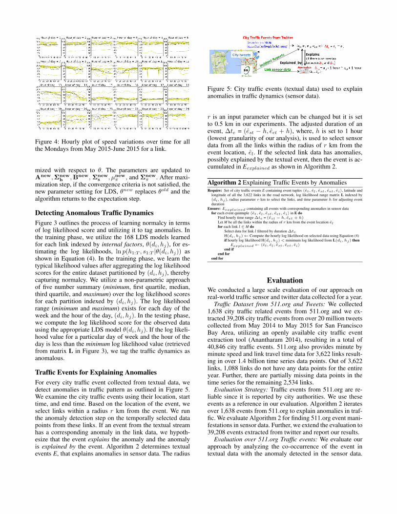
Figure 4: Hourly plot of speed variations over time for allthe Mondays from May 2015-June 2015 for a link.

mized with respect to θ. The parameters are updated toAnew,Σnew

h ,Bnew, Σnews , µnew

π , and Σnewπ . After maxi-

mization step, if the convergence criteria is not satisfied, thenew parameter setting for LDS, θnew replaces θold and thealgorithm returns to the expectation step.

Detecting Anomalous Traffic DynamicsFigure 3 outlines the process of learning normalcy in termsof log likelihood score and utilizing it to tag anomalies. Inthe training phase, we utilize the 168 LDS models learnedfor each link indexed by internal factors, θ(di, hj), for es-timating the log likelihoods, ln p(h1:T , s1:T |θ(di, hj)) asshown in Equation (4). In the training phase, we learn thetypical likelihood values after aggregating the log likelihoodscores for the entire dataset partitioned by (di, hj), therebycapturing normalcy. We utilize a non-parametric approachof five number summary (minimum, first quartile, median,third quartile, and maximum) over the log likelihood scoresfor each partition indexed by (di, hj). The log likelihoodrange (minimum and maximum) exists for each day of theweek and the hour of the day, (di, hj). In the testing phase,we compute the log likelihood score for the observed datausing the appropriate LDS model θ(di, hj). If the log likeli-hood value for a particular day of week and the hour of theday is less than the minimum log likelihood value (retrievedfrom matrix L in Figure 3), we tag the traffic dynamics asanomalous.

Traffic Events for Explaining AnomaliesFor every city traffic event collected from textual data, wedetect anomalies in traffic pattern as outlined in Figure 5.We examine the city traffic events using their location, starttime, and end time. Based on the location of the event, weselect links within a radius r km from the event. We runthe anomaly detection step on the temporally selected datapoints from these links. If an event from the textual streamhas a corresponding anomaly in the link data, we hypoth-esize that the event explains the anomaly and the anomalyis explained by the event. Algorithm 2 determines textualevents E, that explains anomalies in sensor data. The radius

Figure 5: City traffic events (textual data) used to explainanomalies in traffic dynamics (sensor data).

r is an input parameter which can be changed but it is setto 0.5 km in our experiments. The adjusted duration of anevent, ∆te = (est − h, eet + h), where, h is set to 1 hour(lowest granularity of our analysis), is used to select sensordata from all the links within the radius of r km from theevent location, el. If the selected link data has anomalies,possibly explained by the textual event, then the event is ac-cumulated in Eexplained as shown in Algorithm 2.

Algorithm 2 Explaining Traffic Events by AnomaliesRequire: Set of city traffic events E containing event tuples 〈et, el, est, eet, ei〉, latitude and

longitude of all the 3,622 links in the road network, log likelihood range matrix L indexed by(di, hj), radius parameter r km to select the links, and time parameter h for adjusting eventduration

Ensure: Eexplained containing all events with corresponding anomalies in sensor datafor each event quintuple 〈et, el, est, eet, ei〉 in E do

Find hourly time range ∆te = (est − h, eet + h)Let M be all the links within the radius of r km from the event location elfor each link l ∈ M do

Select data for link l filtered by duration ∆teH(di, hj)← Compute the hourly log likelihood on selected data using Equation (4)if hourly log likelihood H(di, hj)< minimum log likelihood from L(di, hj) then

Eexplained←〈et, el, est, eet, ei〉end if

end forend for

EvaluationWe conducted a large scale evaluation of our approach onreal-world traffic sensor and twitter data collected for a year.

Traffic Dataset from 511.org and Tweets: We collected1,638 city traffic related events from 511.org and we ex-tracted 39,208 city traffic events from over 20 million tweetscollected from May 2014 to May 2015 for San FranciscoBay Area, utilizing an openly available city traffic eventextraction tool (Anantharam 2014), resulting in a total of40,846 city traffic events. 511.org also provides minute byminute speed and link travel time data for 3,622 links result-ing in over 1.4 billion time series data points. Out of 3,622links, 1,088 links do not have any data points for the entireyear. Further, there are partially missing data points in thetime series for the remaining 2,534 links.

Evaluation Strategy: Traffic events from 511.org are re-liable since it is reported by city authorities. We use theseevents as a reference in our evaluation. Algorithm 2 iteratesover 1,638 events from 511.org to explain anomalies in traf-fic. We evaluate Algorithm 2 for finding 511.org event mani-festations in sensor data. Further, we extend the evaluation to39,208 events extracted from twitter and report our results.

Evaluation over 511.org Traffic events: We evaluate ourapproach by analyzing the co-occurrence of the event intextual data with the anomaly detected in the sensor data.

Source Total Events No Links Missing Data No Anomalies Anomalies511.org 1,638 201 901 145 391Twitter 39,208 36,436 1942 18 812

Table 1: Evaluation results for all the events using Algo-rithm 2 with parameter setting: h = 1 hour and r = 0.5 km.

Table 1 presents the evaluation summary for all the 1,638511.org events and 39,208 twitter traffic events. Events withno links near them (for r = 0.5 km) are placed under NoLinks. If there are links near an event, with data that may bemissing (for the event duration), then they are characterizedas Missing Data. Links near an event with data are used totag anomalies and the result is placed under No Anomaliesand Anomalies. We call the events corroborated with anoma-lies in any of the link sensor data near the event as being ex-plained. Events without accompanying anomalies in any ofthe link sensor data are called un-explained. For a palatablecomparison, we present percentages of events from 511.organd twitter that explain anomalies in Figure 6. We observe alarger set of links near events from 511.org relative to twitterevents as shown in Figure 6 (bottom). Out of 33% 511.orgevents with complete sensor data, we could explain 72% ofthem. Figure 6 (top) presents a sample output of Algorithm 2after processing 10 events. For events marked in bold, wefound anomalies in traffic dynamics possibly explained bythe event with the following insights: (a) Long-term eventsmay not manifest as anomalies in sensor data. RSLDS nor-malcy model is trained over the entire year of average speedand travel time observations. Long-term events such as con-struction activities may span several months. Since the datawe have is for a year, such long-term events are part of thenormalcy model and may not be tagged anomalous as ob-served in Figure 6 (top). Events, such as accidents and dis-abled vehicles, are short lived events that may manifest asanomalous traffic. (b) Location and start time of the eventmay impact its manifestation in sensor data. Events nearcrowded places would most likely manifest as anomalies.Events occurring during off-peak hours are less likely tomanifest in sensor data compared to the events occurringduring peak-hours. (c) Missing data creates challenges forassociating anomalies with events. Among the 2,534 linkswith data, there is missing data for many days in a year dueto maintenance and sensor failures resulting in decreasedcoverage.

Evaluation over Twitter Traffic Events: Twitter trafficevents are dispersed widely across the city resulting in re-duced or missing links near many events. There are 36,436twitter traffic events with no links near them as shown in Ta-ble 1 due to significantly lower sensor data coverage. Con-sequently, we observe that the coverage can be significantlyimproved by augmenting information from sensor data withthat from twitter events as shown in Figure 6 (bottom). Weexpected a higher twitter traffic event manifestation in sen-sor data since people will most likely report events of signif-icant impact while 511.org reports all possible traffic relatedevents that may have varying impact. Out of 2% twitter traf-fic events with complete sensor data, we could corroborate97% of it with anomalies.

Figure 6: City traffic events with available and missing linkdata and percentage of events explained by Algorithm 2

Scalability Challenges: There are 2,534 links with data.For each link, we learn 168 LDS models by analyzing over1.4 billion data points resulting in a total of 425,712 (=2,534 × 168) LDS models. The size of the traffic datasetis around 30 GB. Learning LDS parameters and the crite-ria for anomaly is computationally expensive. For each linkwith one year of data, we estimated 25 minutes for learningLDS models and 15 minutes for computing the criteria foranomaly, resulting in a total processing time of 40 minutesper link. Extrapolating processing time for all the links, weget 1,689 hours ( 40minutes×2,53460minutes ) (≈2 months). Initial pro-cessing was done with 2.66 GHz, Intel Core 2 Duo processorwith 8 GB main memory. We then exploited inherent “em-barrassing parallelism” to devise a scalable implementationof our approach on Apache Spark (Zaharia et al. 2010) thattakes less than a day. The Apache Spark cluster used in ourevaluation has 864 cores and 17TB main memory.

Conclusion and Future Work

Normal traffic dynamics can be captured using RSLDS, avariant of LDS model, that utilizes domain knowledge tosegment nonlinear traffic dynamics into linear components.Utilizing the normalcy model, we could explain anomaliesin traffic sensor data using traffic events from textual data.We could also associate real-world events that impact trafficby determining anomalies in traffic pattern. Further, a largescale evaluation of our approach on a real-world dataset col-lected for a year corroborated 72% of 511.org events and97% of twitter traffic events in terms of anomalous trafficdynamics. As a future work, RSLDS model capturing tem-poral dynamics can be utilized to study various traffic eventtypes and associated speed and travel time dynamics andpredict traffic dynamics based on the traffic events from tex-tual streams.

AcknowledgmentsThis material is based upon work supported by the NationalScience Foundation under Grant No. EAR 1520870 titled“Hazards SEES: Social and Physical Sensing Enabled Deci-sion Support for Disaster Management and Response”. Anyopinions, findings, and conclusions or recommendations ex-pressed in this material are those of the author(s) and donot necessarily reflect the views of the National ScienceFoundation. We would also like to acknowledge the EU FP7Citypulse project contract number: 609035 for providing abroader motivation for this work.

ReferencesAnantharam, P. 2014. Extracting city traffic events from so-cial streams. https://osf.io/b4q2t/wiki/home/.Anderson, J., and Bell, M. 1997. Travel time estimation inurban road networks. In Intelligent Transportation System,1997. ITSC’97., IEEE Conference on, 924–929. IEEE.Barber, D. 2012. Bayesian reasoning and machine learning.Cambridge University Press.Bishop, C. M. 2006. Pattern recognition and machine learn-ing. springer.Boulos, M. N. K.; Resch, B.; Crowley, D. N.; Breslin, J. G.;Sohn, G.; Burtner, R.; Pike, W. A.; Jezierski, E.; and Chuang,K.-Y. S. 2011. Crowdsourcing, citizen sensing and sen-sor web technologies for public and environmental healthsurveillance and crisis management: trends, ogc standardsand application examples. International journal of health ge-ographics 10(1):67.Chawla, S.; Zheng, Y.; and Hu, J. 2012. Inferring theroot cause in road traffic anomalies. In Data Mining(ICDM), 2012 IEEE 12th International Conference on, 141–150. IEEE.Crooks, A.; Croitoru, A.; Stefanidis, A.; and Radzikowski, J.2013. # earthquake: Twitter as a distributed sensor system.Transactions in GIS 17(1):124–147.Daly, E. M.; Lecue, F.; and Bicer, V. 2013. Westland row whyso slow?: fusing social media and linked data sources for un-derstanding real-time traffic conditions. In Proceedings of the2013 international conference on Intelligent user interfaces,203–212. ACM.De Fabritiis, C.; Ragona, R.; and Valenti, G. 2008. Trafficestimation and prediction based on real time floating car data.In Intelligent Transportation Systems, 2008. ITSC 2008. 11thInternational IEEE Conference on, 197–203. IEEE.Fanaee-T, H., and Gama, J. 2014. Event labeling combiningensemble detectors and background knowledge. Progress inArtificial Intelligence 2(2-3):113–127.Ghahramani, Z., and Hinton, G. E. 1996. Parameter estima-tion for linear dynamical systems. Technical report, TechnicalReport CRG-TR-96-2, University of Totronto, Dept. of Com-puter Science.Goodchild, M. F. 2007. Citizens as sensors: the world ofvolunteered geography. GeoJournal 69(4):211–221.Horvitz, E.; Apacible, J.; Sarin, R.; and Liao, L. 2012.Prediction, expectation, and surprise: Methods, designs, andstudy of a deployed traffic forecasting service. arXiv preprintarXiv:1207.1352.IBM. 2014. Smarter traffic. http://www.ibm.com/smarterplanet/us/en/traffic_congestion/ideas/.

Ko, J., and Guensler, R. L. 2005. Characterization of conges-tion based on speed distribution: a statistical approach usinggaussian mixture model. In Transportation Research BoardAnnual Meeting. Citeseer.Koller, D., and Friedman, N. 2009. Probabilistic graphicalmodels: principles and techniques. MIT press.Lecue, F.; Schumann, A.; and Sbodio, M. L. 2012. Applyingsemantic web technologies for diagnosing road traffic con-gestions. In The Semantic Web–ISWC 2012. Springer. 114–130.Lee, S., and Fambro, D. 1999. Application of subsetautoregressive integrated moving average model for short-term freeway traffic volume forecasting. Transportation Re-search Record: Journal of the Transportation Research Board(1678):179–188.Lee, W.-H.; Tseng, S.-S.; and Tsai, S.-H. 2009. A knowl-edge based real-time travel time prediction system for urbannetwork. Expert Systems with Applications 36(3):4239–4247.Moorthy, C., and Ratcliffe, B. 1988. Short term traffic fore-casting using time series methods. Transportation planningand technology 12(1):45–56.Nagarajan, M.; Sheth, A.; and Velmurugan, S. 2011. Citizensensor data mining, social media analytics and developmentcentric web applications. In Proceedings of the 20th interna-tional conference companion on World wide web, 289–290.ACM.Pattara-Atikom, W.; Pongpaibool, P.; and Thajchayapong, S.2006. Estimating road traffic congestion using vehicle veloc-ity. In ITS Telecommunications Proceedings, 2006 6th Inter-national Conference on, 1001–1004. IEEE.Quinn, J. A.; Williams, C. K.; and McIntosh, N. 2009. Fac-torial switching linear dynamical systems applied to physio-logical condition monitoring. Pattern Analysis and MachineIntelligence, IEEE Transactions on 31(9):1537–1551.Rajkumar, R. R.; Lee, I.; Sha, L.; and Stankovic, J. 2010.Cyber-physical systems: the next computing revolution. InProceedings of the 47th Design Automation Conference, 731–736. ACM.Sakaki, T.; Okazaki, M.; and Matsuo, Y. 2010. Earthquakeshakes twitter users: real-time event detection by social sen-sors. In Proceedings of the 19th international conference onWorld wide web, 851–860. ACM.Sheth, A.; Anantharam, P.; and Henson, C. 2013. Physical-cyber-social computing: An early 21st century approach. In-telligent Systems, IEEE 28(1):78–82.Sun, S.; Zhang, C.; and Yu, G. 2006. A bayesian network ap-proach to traffic flow forecasting. Intelligent TransportationSystems, IEEE Transactions on 7(1):124–132.Wanichayapong, N.; Pruthipunyaskul, W.; Pattara-Atikom,W.; and Chaovalit, P. 2011. Social-based traffic informa-tion extraction and classification. In ITS Telecommunica-tions (ITST), 2011 11th International Conference on, 107–112. IEEE.Zaharia, M.; Chowdhury, M.; Franklin, M. J.; Shenker, S.;and Stoica, I. 2010. Spark: Cluster computing with workingsets. In Proceedings of the 2Nd USENIX Conference on HotTopics in Cloud Computing, HotCloud’10, 10–10. Berkeley,CA, USA: USENIX Association.Zeng, K.; Liu, W.; Wang, X.; and Chen, S. 2013. Traffic con-gestion and social media in china. IEEE Intelligent Systems28(1):72–77.