Using Kinked Budget Sets to Estimate Extensive Margin

Responses: Method and Evidence from the Social Security

Earnings Test

Alexander M. Gelber, Damon Jones, Daniel W. Sacks, and Jae Song∗

October 2017

Abstract

We develop a method for estimating the effect of a kinked budget set on workers’employment de-

cisions, and we use it to estimate the impact of the Social Security Old-Age and Survivors Insurance

(OASI) Annual Earnings Test (AET). The AET reduces OASI claimants’current OASI benefits in pro-

portion to their earnings in excess of an exempt amount. Using a Regression Kink Design and Social

Security Administration data, we document that the discontinuous change in the benefit reduction rate

at the exempt amount causes a corresponding change in the slope of the employment rate. We develop

conditions in a general setting under which we can use such patterns to estimate the elasticity of the

employment rate with respect to the effective average net-of-tax rate. Our resulting elasticity point

estimate for the AET is at least 0.49, suggesting that the AET reduces employment by more than one

percentage point in the group we study.

∗Gelber: UC Berkeley Goldman School of Public Policy and NBER, agelber@berkeley.edu; Jones: University of Chicago,Harris School of Public Policy and NBER, damonjones@uchicago.edu; Sacks: Indiana University, Kelley School of Business,dansacks@indiana.edu; Song: Social Security Administration, jae.song@ssa.gov. This research was supported by the U.S.Social Security Administration through grant #RRC08098400-06-00 to the National Bureau of Economic Research as part ofthe SSA Retirement Research Consortium and by grant #G-2015-14005 from the Alfred P. Sloan Foundation. The findingsand conclusions expressed are solely those of the authors and do not represent the views of SSA, any agency of the FederalGovernment, or the NBER. We also thank the UC Berkeley IRLE, CGIF, and Burch Center for research support. We areextremely grateful to David Pattison for running our early code on the data. We thank David Card, Raj Chetty, Jim Cole, JulieCullen, Rebecca Diamond, Avi Feller, Jon Gruber, Hilary Hoynes, Pat Kline, Rafael Lalive, Emmanuel Saez, Håkan Selin, JoelSlemrod, and seminar participants at Brookings, Case Western Reserve, Cornell, Dartmouth, DePaul, Duke, Maryland, NBER,Notre Dame, NYU, SIEPR, UC Berkeley, UC Davis, University of Chicago, UIC, UIUC, and UVa for helpful comments. Allerrors are our own.

1 Introduction

Non-linear price schedules are common across a wide variety of economic applications, including labor supply

(e.g. Hausman, 1981), electricity demand (e.g. Ito, 2014), health insurance (e.g. Einav, Finkelstein, and

Schrimpf, 2015), and retirement savings (e.g. Bernheim, Fradkin, and Popov, 2015). Taxes and government

transfers in particular often create kink points, discontinuous changes in the marginal incentive to earn

or work more. For example, many means-tested government transfer programs reduce transfer benefits

as income rises above threshold levels, and the individual income tax in many countries also generates a

piecewise linear budget set with kinks at each point at which the marginal tax rate (MTR) jumps. Previous

literature has developed methods for explicitly using kink points or notches in the effective tax schedule to

estimate responses at the intensive margin, the choice of earnings or hours worked conditional on working

(e.g. Burtless and Hausman, 1978; Hausman, 1981; Saez, 2010; Chetty, Friedman, Olsen, and Pistaferri,

2011; Kleven and Waseem, 2013; see the review in Kleven, 2016). However, the welfare implications of

tax and transfer policies depend not only on the magnitude of intensive margin responses, but also on the

degree of responses at the extensive margin, the choice of whether or not to be employed (Diamond, 1980;

Saez, 2002; Eissa, Kleven, and Kreiner, 2008). More generally, the effects of incentives on earnings and the

employment rate are both key questions across several fields in economics.

In this paper, we develop a method for estimating the effects of kinked budget sets on workers’extensive

margin decisions. Our method relies on clear patterns in data: under the conditions we specify, a kink

in a budget set leads to a kink in the employment rate. Specifically, suppose individuals face fixed costs

of employment such as commuting costs (Cogan, 1981), and consider the probability of employment as a

function of the desired earnings individuals would choose if employed. If the individual faces a linear budget

set, this function should presumably be smooth (continuously differentiable), as illustrated in the dashed

line in Figure 1. Now consider a budget set with a convex kink at which the effective marginal tax rate

discontinuously rises. Figure 2 shows that in this case the slope of the average net-of-tax rate (ANTR)

decreases discontinuously at the kink point.1 The ANTR is defined as the fraction of an individual’s income

that the individual keeps net of taxes and benefit reduction when earning a positive amount rather than

earning zero, reflecting the individual’s incentive to be employed. In this environment, we show that there

should robustly be a discontinuous decrease at the kink point in the slope of the probability of employment

among individuals who are constrained from making small, intensive margin adjustments. This is illustrated

in the solid line in Figure 1. Intuitively, these intensive margin frictions prevent individuals from locating

at the kink even if they might otherwise like to do so under the kinked budget constraint, driving them to

non-employment instead and fueling a discontinuous decrease in the slope of employment.2

Thus, observing such a change in slope represents a novel type of evidence that a kinked budget set has

an extensive margin effect. Our assumptions are therefore testable, as this change in slope should arise if1 Formally, for a tax schedule T (z), we define the ANTR as ANTR ≡ 1− T (z) /z, where z is pre-tax earnings.2Our method also applies at non-convex kinks: the slope of the employment rate discontinuously increases for those constrained

from adjusting away from non-convex kinks.

1

individuals face fixed costs of employment as well as intensive margin frictions. This prediction does not

rely on parametric assumptions on the utility function, nor on assuming a representative agent; indeed the

distribution of employment responses in the population, as well as other distributional assumptions, are left

unrestricted. Using a Regression Kink Design (RKD), we can estimate the change in slope of the employment

rate (Nielson, Sorenson, and Taber, 2010; Card, Lee, Pei, and Weber, 2015), which reflects average extensive

margin effects for those near the budget set kink.

The elasticity of participation with respect to the ANTR– the parameter relevant for welfare analysis

(Eissa, Kleven, and Kreiner, 2008)– can be expressed as a function of the change in the slope of the employ-

ment rate at the kink, as well as other observable moments in the data. All else equal, the larger the change

in the slope of employment at the kink point, the larger the elasticity of employment with respect to the

ANTR. If some individuals do not face such frictions and some do, then we estimate a lower bound on the

average elasticity among both of these two groups without making parametric or distributional assumptions.

We suggest that this method for estimating (a lower bound on) extensive margin elasticities is valid without

such assumptions not only in the case of employment (i.e. a corner solution in leisure demand), but also in

the case of demand for other commodities in the presence of fixed costs of extensive margin decisions as well

as intensive margin frictions.

One collection of prior literature explicitly uses kinked budget sets to estimate intensive margin responses,

while abstracting from the extensive margin that we study (e.g. Burtless and Hausman, 1978; Hausman,

1981; Saez, 2010; Chetty, Friedman, Olsen, and Pistaferri, 2011; Kleven and Waseem, 2013; Kleven, 2016).

Previous literature on the effect of the marginal incentives to be employed on extensive margin employment

decisions, including the literature based on kinks, has generally imposed parametric restrictions to generate

labor supply estimates (Manski, 2014), or has not explicitly related causal responses to the budget constraint

(Blundell and MaCurdy, 1999). For example, prior literature contains estimates of extensive margin responses

to employment incentives under the distributional assumptions in Tobit or discrete choice models (McDonald

and Moffi tt, 1980; Moffi tt, 1983; Hoynes, 1996; Keane and Moffi tt, 1998; Blundell and Shephard, 2012; see the

surveys in Keane, 2011, or Saez, Slemrod, and Giertz, 2012). Similarly, Alpert and Powell (2014) develop

a method that can be used when capital and labor income are both observed under certain restrictions

on functional forms. Other papers have performed program evaluations of such effects using randomized

experiments (e.g. Bitler, Gelbach, and Hoynes, 2006) or other techniques such as difference-in-differences

(e.g. Eissa and Liebman, 1996), but with empirical models that do not explicitly take into account how

the data relate to the budget constraint (Blundell and MaCurdy, 1999). We specify the conditions under

which our method can be used, and our model allows us to be explicit about the about the population and

parameter that our elasticity refers to.

Two recent papers have investigated the effects of a notch– rather than the kinked budget set that is

our focus– on extensive margin decisions in very different contexts than ours. Kleven, Landais, Saez, and

Schultz (2014) explore the effect of a notch on migration using quasi-linear utility, and Kopczuk and Munroe

2

(2015) show that a housing tax notch creates “unraveling”of productive matches within a bargaining model

for the particular housing context. Our work develops methods applicable in the context of a general budget

set kink, with an application to the employment decision.3

None of these existing methods applies the newly developed RKD design in the novel context of explicitly

using kinks in budget sets to estimate extensive margin labor supply or earnings responses.4 Thus, a key

feature of our method is that its central prediction can be transparently confirmed in a simple graph of the

data showing whether the slope of the employment rate changes discontinuously at the kink. Our method

explicitly focuses on discontinuities in the data to drive the results. As our empirical method is valid under

a different set of assumptions than alternative methods for estimating extensive margin responses, we see

our method as complementary to other approaches.

Substantively, we apply our method to show that extensive margin responses are important in the context

of the Social Security Old-Age and Survivors Insurance (OASI) Annual Earnings Test (AET). Although we

focus on the AET, we also explain how our method can be used in other contexts, and we show empirically

that in a broader sample of ages– not just older Americans subject to the AET– conditions hold that allow

our method to be used. The AET reduces OASI claimants’current OASI benefits as a proportion of earnings

in excess of an exempt amount. For example, for OASI claimants aged 62 to the Normal Retirement Age

(NRA) of 66.17 in 2017, current OASI benefits are reduced by one dollar for every additional two dollars

earned above $16,920. This could reduce OASI claimants’ incentives for additional work. Reductions in

current benefits due to the AET sometimes lead to increases in later benefits; nonetheless, as we discuss,

several factors may explain why individuals’earnings still respond to the AET.

The AET is a natural context for studying the extensive margin effects of kinks. The AET is a significant

factor affecting the income of many older Americans. The AET’s large benefit reduction rate (BRR) can

lead to a large budget set kink, suggesting that the AET could have important impacts on employment that

policy-makers wish to understand. Particularly as the economy-wide employment-to-population ratio has

fallen by over four percentage points since its peak in 2000 (Aaronson et al., 2014), many policy makers are

interested in ways to affect employment rates (Abraham and Kearney, 2017), including potential changes to

the AET (Tergesen, 2016). Indeed, the AET is a leading candidate in helping to explain the upward spike in

the hazard of retirement at age 62 (Gruber and Wise 1999). The importance of the AET is now increasing

as the NRA gradually rises from 65 for those born in 1937 and earlier, to 67 for those born in 1960 and later,

exposing more OASI claimants to the AET. Even when the NRA was 65.5 for the youngest OASI primary

beneficiaries in the latest year of the available micro-data in 2003, the AET led to a total of $4.3 billion

3A small literature has developed non-parametric methods for estimating a different parameter, or in a substantially different context.Blomquist, Kumar, Liang, and Newey (2015) non-parametrically estimate the effect of a non-linear budget set on expected labor income,without separating the intensive and extensive margin responses that are necessary for welfare evaluation. In a welfare program creatingkinks and notches, as well as under-reporting of income, welfare stigma, and hassle costs of welfare work requirements, Kline and Tartari(2016) develop non-parametric bounds on labor supply responses in the context of the particular features of their setting, whereas ourpaper focuses on behavior around a general kink.

4 In Austria, Manoli and Weber (2016) use an RKD to study retirement decisions relying on a Saez (2010)-type model of intensivemargin bunching in retirements at the retirement age, while Manoli and Weber (forthcoming) study bunching in retirements at notchescreated by severance payments. Similarly, Card et al. (2015) and Card et al. (2016) use an RKD to study the effect of unemploymentbenefits on unemployment, but their model features an unemployment benefit that is a kinked function of past earnings, as opposed toa kink in the budget constraint itself.

3

in current benefit reductions for around 538,000 beneficiaries, thus substantially affecting benefits and their

timing.5

To estimate the employment effects of the AET, we use Social Security Administration (SSA) data on

a 25 percent random sample of the U.S. population in birth cohorts 1918 to 1923 over the years 1978 to

1987.6 These data cover 11,397,336 observations of calendar year earnings and other information on 1,424,667

individuals in our full sample. Using an RKD, we uncover a novel fact: as a function of past earnings–

which captures desired earnings as we verify– the slope of the employment rate among 63 to 64 year-olds

discontinuously decreases around the budget set kink created by the AET at the exempt amount.7 We

conduct several placebo and other robustness checks to verify that we have found a true effect on earnings,

as opposed to an underlying nonlinearity in the employment rate.

A baseline specification shows that the point estimate of the elasticity of employment with respect to the

ANTR is at least 0.49.8 Simulations relying on these estimates show that eliminating the AET would cause

an increase in the annual employment rate at ages 63 to 64 of 1.4 percentage points in the group we study

near the kink, reflecting a 2.5 percent increase in employment. Using our extensive margin elasticity from this

paper, as well as the AET intensive margin elasticities from Gelber, Jones, and Sacks (2013), we calculate

that earnings in the group we study decrease by 9.8 percent due to the AET. Of the total earnings reductions

due to the AET, 27.6 percent are associated with extensive margin exit decisions. Our model and results

therefore highlight both the potential importance of the AET to older workers’earnings and employment

decisions, as well as the importance of the extensive margin responses in addition to the intensive margin

responses around the kink that are the focus of much recent literature following Saez (2010).

Our new estimates of the effect of the AET on employment relate to long lines of previous research on

the effect of Social Security and other types of pensions on retirement or employment decisions (see the

literature review in Blundell, French, and Tetlow, 2016). With respect to the AET in particular, much of

the previous literature has focused on the policy’s intensive margin effect (e.g. Burtless and Moffi tt, 1985;

Friedberg, 1998; Friedberg, 2000; Song and Manchester, 2007; Gelber, Jones, and Sacks, 2013), typically

finding moderate substitution elasticities at the intensive margin. Given the clear but moderate responses

at the intensive margin, it is arguably surprising that nearly all prior studies find little evidence of extensive

margin responses– particularly since the elderly are often on the margin of whether to retire and therefore

may be especially sensitive to extensive margin incentives (e.g. French, 2005). Indeed, much of the earlier

empirical literature on the AET concludes that the policy has little meaningful effect on the labor supply of

5 If earnings and/or employment are reduced by the AET, then this calculated reduction in benefits reflects a lower bound on thereduction in current benefits we would hypothetically observe if earnings and employment were inert in response to the AET.

6 For our calculation of the $4.3 billion aggregate benefit reduction alone, we use the Benefits and Earnings Public Use File onepercent population sample, because this file has information on all birth cohorts until the more recent year 2003 that illustrates theaggregate benefit reduction better after the NRA had risen above 65. We use our 25 percent random sample of administrative datafrom 1978 to 1987 everywhere else because these data allow much more statistical power to perform the other estimates in the paper.

7We focus on 63 to 64 year-olds for several reasons: this group is relevant to policy, as the AET currently applies to this group butnot to those over NRA; this is the youngest group sub ject to the AET for which measured employment would be affected by the AET,as we explain in detail later; and thus this is the group for which age 60 earnings represents the best proxy for desired earnings.

8 For consistency with the previous literature on kink points that has focused on the effect of taxation, we sometimes use “tax” asshorthand for “tax-and-transfer,” as in our use of the term “ANTR” to apply to the AET, while recognizing that the AET reducesSocial Security benefits and is not administered through the tax system.

4

older men.9 More recent work has examined the effect of the AET on employment decisions using a difference-

in-differences framework. Several of these papers find little evidence for an effect on the employment rate

(Gruber and Orszag, 2003; Song, 2004; Song and Manchester, 2007; Haider and Loughran, 2008), while

Friedberg and Webb (2009) find a significant effect in some specifications in the Current Population Survey.10

We interpret our evidence as showing a clear and robust impact of the AET on the annual employment

rate, in contrast to the bulk of previous literature. The combination of a large administrative dataset with

individual-level microdata (also used in various forms in Song, 2004, Song and Manchester, 2007, and Haider

and Loughran, 2008) and our novel identification strategy based on discontinuities leads to precise estimates

of sizeable elasticities. Our paper is the first that has estimated a significant impact of the AET at the

extensive margin through explicitly modeling individuals’budget sets. However, we estimate the effect of

the AET on those locating near the exempt amount in the policy-relevant 63 to 64 year-old group to which

the AET currently applies– a younger group than those studied in the difference-in-differences literature

cited above– and thus our results are not directly comparable to this previous literature.

The paper proceeds as follows. Section 2 presents our model. Section 3 describes the policy environment.

Section 4 explains our empirical strategy. Section 5 discusses the data. Section 6 presents empirical evidence

on the response to the AET and performs counterfactual simulations. Section 7 concludes.

2 Model

We begin by presenting a model of how a kink in the budget set impacts an individual’s decision of whether

or not to have a positive amount of earnings, which we refer to as the “employment”decision. In particular,

we explore under what conditions the introduction of a kink in the effective tax schedule should cause a

corresponding kink in the employment rate.11 Throughout, we make use of a potential outcomes framework

(Rubin, 1974). We index two potential states of the world by j ∈ {0, 1}. In state 0 individuals face a

linear tax τ0, i.e. T0 (z) = τ0z, where Tj (·) denotes their tax liability in state j and z denotes their pre-tax

earnings. Alternatively, in state 1 the tax schedule exhibits a kink at z∗:

T1(z) =

τ0z, if z < z∗

τ0z∗ + τ1 (z − z∗) if z ≥ z∗

(1)

In our application we interpret z as earnings and T as a tax schedule, but an analogous model should apply

to consumption of any good (or “bad”) under a price schedule with a convex kink.

Following much previous literature on employment responses to kinks or notches (e.g. Hausman, 1981;

Saez, 2010; Kleven and Waseem, 2013), we begin with a static model in which individuals’utility depends

on consumption and earnings, u (c, z;n), where the partial effect of an increase in z on utility is negative

9 See Viscusi (1979), Burtless and Moffi t (1985), Gustman and Steinmeier (1985, 1991), Vroman (1985), Honig and Reimers (1989),and Leonesio (1990).1 0Examining the effects of earnings tests in other countries using difference-in-differences designs, Baker and Benjamin (1999) find a

significant effect of the Canadian earnings test on weeks worked per year but no significant effect on employment at some point duringthe year, and Disney and Smith (2002) find inconclusive evidence on the impact of the U.K. earnings test on the employment rate.1 1To clarify, we use “kink” in two senses– both to describe a discontinuity in the effective marginal tax rate in the budget set, and

to describe a discontinuity in the slope of an outcome variable (in our case the employment rate).

5

as it requires effort to increase earnings, and the partial effect of an increase in c on utility is positive. We

assume u (·) is a function of class C2. As in Saez (2010) and much subsequent literature, we model the

determination of earnings, rather than hours worked, as earnings (but not hours worked) are observed in

many administrative datasets. However, our method can easily be adapted to apply to the determination

of hours worked. Our index of “ability” is n; the marginal rate of substitution of c for z is decreasing in n

at all levels of c and z.12 To simplify the model for the time being, we assume that individuals maximize

utility subject to a static budget constraint:

cnj = znj − Tj (znj) (2)

where znj is realized earnings for an individual with ability n in state j. At an interior solution, the first-order

condition, (1 − T ′j (z))uc + uz ≡ 0, implicitly defines the earnings supply function (we suppress subscripts

here as shorthand).

2.1 Effect of a Kink at the Intensive Margin

Given this setup, we first briefly review the intensive margin effect of a kink. As shown in Saez (2010),

a kinked budget set leads to a discontinuity in the earnings density at the kink due to intensive margin

responses. Assuming a smooth distribution of ability n, a range of individuals who would earn between z∗

and z∗ + ∆z∗ in state 0 will respond in state 1 by reducing earnings to the kink at z∗. This is referred to as

“bunching”at the kink. The reduction in earnings ∆z∗ of the “marginal buncher”– i.e. the buncher who

earns the most, z∗ + ∆z∗, in state 0– can be related to the size of the change in the marginal tax rate at

the kink, dτ ≡ τ1 − τ0, in order to estimate an intensive margin elasticity (Saez, 2010).

2.2 Extensive Margin Responses

In addition to the intensive margin response that much recent literature has focused on, individuals may

also respond at the extensive margin. In the model in Section 2.1, preferences and budget sets are convex,

which restricts a small tax change only to affect the choice between zero and infinitesimally small earnings

supply (e.g. Kleven and Kreiner, 2005). To capture the realistic pattern of potential entry to or exit from

non-trivial levels of earnings, we introduce a fixed cost of employment (Cogan, 1981; Eissa, Kleven, and

Kreiner, 2008). Utility conditional on working is now given by:

u (cnj , znj ;n) = v (cnj , znj ;n)− qnj · 1 {znj > 0} (3)

where j ∈ {0, 1} indexes the state of the world, and the state-specific, additively separable fixed cost of

employment, qnj , is drawn from a distribution with CDF G (q|n) and pdf g (q|n). If an agent does not

work, she receives a reservation level of utility of u(c0, 0;n

)= v0 in either state of the world.13 ,14 We often

1 2This implies a standard single-crossing property assumed in these models, which generates rank preservation in earnings, conditionalon earning a positive amount.1 3Without loss of generality, the outside option, v0, does not vary with n or j. This is because cross-sectional and state-specific

variation in the outside option is not separately identified from the fixed cost of entry qnj . We therefore collapse all such variation intothe fixed cost of entry. Similarly, we can interpret our framework as accommodating extensive margin frictions in the form of a fixedcost, as such frictions could be considered part of the fixed cost of working.1 4Writing the fixed cost q as separable from v, as in (3) above, simplifies the exposition. Without loss of generality, this model

is equivalent to a model in which these are not separable per se , and instead we express utility simply as v (c, z;n). Letting c0n be

6

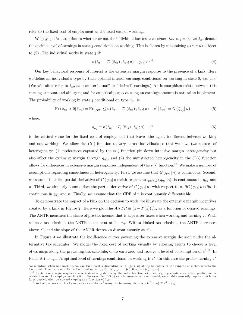
refer to the fixed cost of employment as the fixed cost of working.

We pay special attention to whether or not the individual locates at a corner, i.e. znj = 0. Let znj denote

the optimal level of earnings in state j conditional on working. This is chosen by maximizing u (c, z;n) subject

to (2). The individual works in state j if:

v (znj − Tj (znj) , znj ;n)− qnj > v0 (4)

Our key behavioral response of interest is the extensive margin response to the presence of a kink. Here

we define an individual’s type by their optimal interior earnings conditional on working in state 0, i.e. zn0.

(We will often refer to zn0 as “counterfactual”or “desired”earnings.) An isomorphism exists between this

earnings amount and ability n, and for empirical purposes using an earnings amount is natural to implement.

The probability of working in state j conditional on type zn0 is:

Pr (znj > 0| zn0) = Pr(qnj ≤ v (znj − Tj (znj) , znj ;n)− v0

∣∣ zn0

)= G

(qnj∣∣n) (5)

where:

qnj ≡ v (znj − Tj (znj) , znj ;n)− v0 (6)

is the critical value for the fixed cost of employment that leaves the agent indifferent between working

and not working. We allow the G(·) function to vary across individuals so that we have two sources of

heterogeneity: (1) preferences captured by the v(·) function pin down intensive margin heterogeneity but

also affect the extensive margin through qn1, and (2) the unrestricted heterogeneity in the G (·) function

allows for differences in extensive margin responses independent of the v (·) function.15 We make a number of

assumptions regarding smoothness in heterogeneity. First, we assume that G (qnj |n) is continuous. Second,

we assume that the partial derivative of G (qnj |n) with respect to qnj , g (qnj |n), is continuous in qnj and

n. Third, we similarly assume that the partial derivative of G (qnj |n) with respect to n, ∂G (qnj |n) /∂n, is

continuous in qnj and n. Finally, we assume that the CDF of n is continuously differentiable.

To demonstrate the impact of a kink on the decision to work, we illustrate the extensive margin incentives

created by a kink in Figure 2. Here we plot the ANTR ≡ (z − T (z)) /z, as a function of desired earnings.

The ANTR measures the share of pre-tax income that is kept after taxes when working and earning z. With

a linear tax schedule, the ANTR is constant at 1 − τ0. With a kinked tax schedule, the ANTR decreases

above z∗, and the slope of the ANTR decreases discontinuously at z∗.

In Figure 3 we illustrate the indifference curves governing the extensive margin decision under the al-

ternative tax schedules. We model the fixed cost of working visually by allowing agents to choose a level

of earnings along the prevailing tax schedule, or to earn zero and receive a level of consumption of c0.16 In

Panel A the agent’s optimal level of earnings conditional on working is z∗. In this case she prefers earning z∗

consumption when not working, we can then posit a discontinuity in v (c, z;n) at the boundary of the support of z that reflects thefixed cost. Thus, we can define a fixed cost qn as: qn ≡ limz−>0+

[v(c0n, 0;n

)− v

(c0n, z, n

)].

1 5 If extensive margin responses were instead only driven by the value function v (·), we might generate unexpected predictions orrestrictions on the employment function. For example, if G (·) were homogeneous in our model, we would necessarily require that laborforce participation be upward sloping as a function of zn0.1 6 For the purposes of this figure, we can redefine c0 using the following identity u

(c0, 0;n

)≡ v0 + qnj .

7

to earning zero. Her response to the kink is simply a reduction in earnings. In Panel B, the agent similarly

has optimal earnings of z∗ conditional on having positive earnings. In this case the individual’s preferences

lead her to earn zero rather than earning at the kink. Next we formally explore such responses.

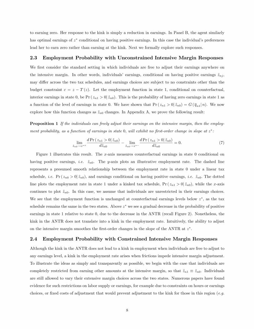
2.3 Employment Probability with Unconstrained Intensive Margin Responses

We first consider the standard setting in which individuals are free to adjust their earnings anywhere on

the intensive margin. In other words, individuals’ earnings, conditional on having positive earnings znj ,

may differ across the two tax schedules, and earnings choices are subject to no constraints other than the

budget constraint c = z − T (z). Let the employment function in state 1, conditional on counterfactual,

interior earnings in state 0, be Pr (zn1 > 0| zn0). This is the probability of having zero earnings in state 1 as

a function of the level of earnings in state 0. We have shown that Pr (zn1 > 0| zn0) = G (qn1|n). We now

explore how this function changes as zn0 changes. In Appendix A, we prove the following result:

Proposition 1 If the individuals can freely adjust their earnings on the intensive margin, then the employ-

ment probability, as a function of earnings in state 0, will exhibit no first-order change in slope at z∗:

limzn0→z∗+

dPr (zn1 > 0| zn0)

dzn0− limzn0→z∗−

dPr (zn1 > 0| zn0)

dzn0= 0. (7)

Figure 1 illustrates this result. The x-axis measures counterfactual earnings in state 0 conditional on

having positive earnings, i.e. zn0. The y-axis plots an illustrative employment rate. The dashed line

represents a presumed smooth relationship between the employment rate in state 0 under a linear tax

schedule, i.e. Pr (zn0 > 0| zn0), and earnings conditional on having positive earnings, i.e. zn0. The dotted

line plots the employment rate in state 1 under a kinked tax schedule, Pr (zn1 > 0| zn0), while the x-axis

continues to plot zn0. In this case, we assume that individuals are unrestricted in their earnings choices.

We see that the employment function is unchanged at counterfactual earnings levels below z∗, as the tax

schedule remains the same in the two states. Above z∗ we see a gradual decrease in the probability of positive

earnings in state 1 relative to state 0, due to the decrease in the ANTR (recall Figure 2). Nonetheless, the

kink in the ANTR does not translate into a kink in the employment rate. Intuitively, the ability to adjust

on the intensive margin smoothes the first-order changes in the slope of the ANTR at z∗.

2.4 Employment Probability with Constrained Intensive Margin Responses

Although the kink in the ANTR does not lead to a kink in employment when individuals are free to adjust to

any earnings level, a kink in the employment rate arises when frictions impede intensive margin adjustment.

To illustrate the ideas as simply and transparently as possible, we begin with the case that individuals are

completely restricted from earning other amounts at the intensive margin, so that zn1 ≡ zn0. Individuals

are still allowed to vary their extensive margin choices across the two states. Numerous papers have found

evidence for such restrictions on labor supply or earnings, for example due to constraints on hours or earnings

choices, or fixed costs of adjustment that would prevent adjustment to the kink for those in this region (e.g.

8

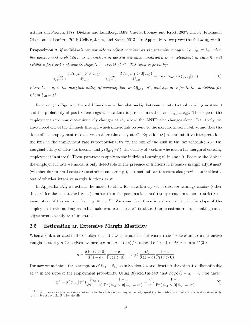
Altonji and Paxson, 1988; Dickens and Lundberg, 1993; Chetty, Looney, and Kroft, 2007; Chetty, Friedman,

Olsen, and Pistaferri, 2011; Gelber, Jones, and Sacks, 2013). In Appendix A, we prove the following result:

Proposition 2 If individuals are not able to adjust earnings on the intensive margin, i.e. zn1 ≡ zn0, then

the employment probability, as a function of desired earnings conditional on employment in state 0, will

exhibit a first-order change in slope (i.e. a kink) at z∗. This kink is given by:

limzn0→z∗+

dPr (zn1 > 0| zn0)

dzn0− limzn0→z∗−

dPr (zn1 > 0| zn0)

dzn0= −dτ · λn∗ · g (qn∗1|n∗) (8)

where λn ≡ vc is the marginal utility of consumption, and qn∗1, n∗, and λn∗ all refer to the individual for

whom zn0 = z∗.

Returning to Figure 1, the solid line depicts the relationship between counterfactual earnings in state 0

and the probability of positive earnings when a kink is present in state 1 and zn1 ≡ zn0. The slope of the

employment rate now discontinuously changes at z∗, where the ANTR also changes slope. Intuitively, we

have closed one of the channels through which individuals respond to the increase in tax liability, and thus the

slope of the employment rate decreases discontinuously at z∗. Equation (8) has an intuitive interpretation:

the kink in the employment rate is proportional to dτ , the size of the kink in the tax schedule; λn∗ , the

marginal utility of after-tax income; and g (qn∗1|n∗), the density of workers who are on the margin of entering

employment in state 0. These parameters apply to the individual earning z∗ in state 0. Because the kink in

the employment rate we model is only detectable in the presence of frictions in intensive margin adjustment

(whether due to fixed costs or constraints on earnings), our method can therefore also provide an incidental

test of whether intensive margin frictions exist.

In Appendix B.1, we extend the model to allow for an arbitrary set of discrete earnings choices (other

than z∗ for the constrained types), rather than the parsimonious and transparent– but more restrictive–

assumption of this section that zn1 ≡ zn0.17 We show that there is a discontinuity in the slope of the

employment rate as long as individuals who earn near z∗ in state 0 are constrained from making small

adjustments exactly to z∗ in state 1.

2.5 Estimating an Extensive Margin Elasticity

When a kink is created in the employment rate, we may use this behavioral response to estimate an extensive

margin elasticity η for a given average tax rate a ≡ T (z) /z, using the fact that Pr (z > 0) = G (q):

η ≡ dPr (z > 0)

d (1− a)

1− aPr (z > 0)

= g (q)∂q

∂ (1− a)

1− aPr (z > 0)

For now we maintain the assumption of zn1 ≡ zn0 as in Section 2.4 and denote β the estimated discontinuity

at z∗ in the slope of the employment probability. Using (8) and the fact that ∂q /∂ (1− a) = λz, we have:

η∗ = g (qn∗1|n∗)∂qn∗1

∂ (1− a)

1− aPr (zn1 > 0| zn0 = z∗)

=β

α· 1− a

Pr (zn1 > 0| zn0 = z∗)(9)

1 7 In fact, one can allow for some continuity in the choice set as long as, loosely speaking, individuals cannot make adjustments exactlyto z∗. See Appendix B.1 for details.

9

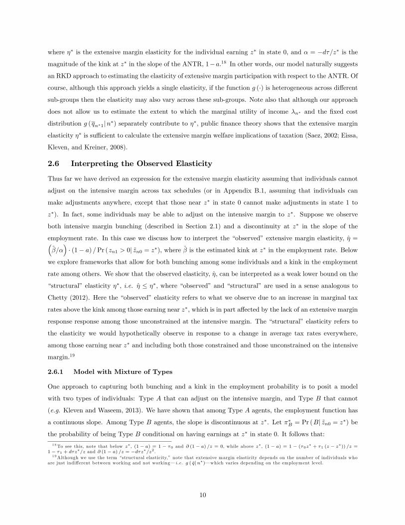
where η∗ is the extensive margin elasticity for the individual earning z∗ in state 0, and α = −dτ/z∗ is the

magnitude of the kink at z∗ in the slope of the ANTR, 1−a.18 In other words, our model naturally suggests

an RKD approach to estimating the elasticity of extensive margin participation with respect to the ANTR. Of

course, although this approach yields a single elasticity, if the function g (·) is heterogeneous across different

sub-groups then the elasticity may also vary across these sub-groups. Note also that although our approach

does not allow us to estimate the extent to which the marginal utility of income λn∗ and the fixed cost

distribution g (qn∗1|n∗) separately contribute to η∗, public finance theory shows that the extensive margin

elasticity η∗ is suffi cient to calculate the extensive margin welfare implications of taxation (Saez, 2002; Eissa,

Kleven, and Kreiner, 2008).

2.6 Interpreting the Observed Elasticity

Thus far we have derived an expression for the extensive margin elasticity assuming that individuals cannot

adjust on the intensive margin across tax schedules (or in Appendix B.1, assuming that individuals can

make adjustments anywhere, except that those near z∗ in state 0 cannot make adjustments in state 1 to

z∗). In fact, some individuals may be able to adjust on the intensive margin to z∗. Suppose we observe

both intensive margin bunching (described in Section 2.1) and a discontinuity at z∗ in the slope of the

employment rate. In this case we discuss how to interpret the “observed”extensive margin elasticity, η =(β/α

)· (1− a) /Pr (zn1 > 0| zn0 = z∗), where β is the estimated kink at z∗ in the employment rate. Below

we explore frameworks that allow for both bunching among some individuals and a kink in the employment

rate among others. We show that the observed elasticity, η, can be interpreted as a weak lower bound on the

“structural”elasticity η∗, i.e. η ≤ η∗, where “observed”and “structural”are used in a sense analogous to

Chetty (2012). Here the “observed”elasticity refers to what we observe due to an increase in marginal tax

rates above the kink among those earning near z∗, which is in part affected by the lack of an extensive margin

response response among those unconstrained at the intensive margin. The “structural”elasticity refers to

the elasticity we would hypothetically observe in response to a change in average tax rates everywhere,

among those earning near z∗ and including both those constrained and those unconstrained on the intensive

margin.19

2.6.1 Model with Mixture of Types

One approach to capturing both bunching and a kink in the employment probability is to posit a model

with two types of individuals: Type A that can adjust on the intensive margin, and Type B that cannot

(e.g. Kleven and Waseem, 2013). We have shown that among Type A agents, the employment function has

a continuous slope. Among Type B agents, the slope is discontinuous at z∗. Let π∗B = Pr (B| zn0 = z∗) be

the probability of being Type B conditional on having earnings at z∗ in state 0. It follows that:

1 8To see this, note that below z∗, (1− a) = 1 − τ0 and ∂ (1− a) /z = 0, while above z∗, (1− a) = 1 − (τ0z∗ + τ1 (z − z∗)) /z =

1− τ1 + dτz∗/z and ∂ (1− a) /z = −dτz∗/z2.1 9Although we use the term “structural elasticity,” note that extensive margin elasticity depends on the number of individuals who

are just indifferent between working and not working– i.e. g ( q|n∗)– which varies depending on the employment level.

10

limzn0→z∗+

dPr (zn1 > 0| zn0)

dzn0− limzn0→z∗−

dPr (zn1 > 0| zn0)

dzn0= −π∗B · dτ · gB (qn∗1|n∗) (10)

where gB (·) is the pdf of fixed costs among Type B agents. In this sense, our estimate of the extensive

margin elasticity is attenuated by a factor π∗B and can therefore be considered a weak lower bound on the

elasticity among Type B agents with state 0 earnings z∗. Among Type A agents who earn above z∗ in state

0, there may also be a response to the kink that increases gradually above z∗ as in Figure 1, but our method

only picks up responses among Type B agents.20 Nonetheless, the observed elasticity is a lower bound on

the elasticity among all of those earning z∗ in state 1:

η =β

α· 1− a

Pr (zn1 > 0| zn0 = z∗)= π∗B · η∗B ≤ π∗A · η∗A + π∗B · η∗B = η∗ (11)

In principle it would be possible to use the observed elasticity η, together with an estimate of the

fraction constrained π∗B , to estimate the structural elasticity among constrained agents, η∗B = η/π∗B . However,

estimating π∗B requires more restrictive assumptions, including assuming that types A and B have the same

distribution of q and n, as we explain in Appendix B.2. Our observed elasticity remains of interest regardless

of the underlying proportion of agents displaying different types of behavior, both in the sense that policy-

makers are interested in the raw employment effects of changing policy parameters like the average tax rate,

and in the sense that it reflects a lower bound on the structural elasticity.

2.6.2 Model with a Fixed Cost of Intensive Margin Adjustment

In an alternative model of intensive margin frictions, individuals face a fixed cost of adjusting earnings on

the intensive margin in response to variation in the tax schedule (see Gelber, Jones, and Sacks, 2013, for a

detailed exposition of this model). Such frictions could reflect a variety of factors, including lack of knowledge

of a tax regime, the cost of negotiating a new contract with an employer, or the time and financial cost of

job search. With a fixed intensive margin adjustment cost individuals will only adjust if the utility gain of

intensive margin adjustment exceeds the fixed cost. Recall that for individuals earning zn0 < z∗ there is no

change in the tax schedule from state 0 to state 1, and therefore zn1 = zn0. Also, due to the fixed cost of

intensive margin adjustment individuals with zn0 > z∗ for whom zn0 is suffi ciently close to z∗ will also prefer

to keep earnings fixed across the two tax schedules. The reason is that the utility gain from adjusting on the

intensive margin converges to zero as zn0 approaches z∗: the optimal level of earnings is z∗ in state 1 for this

group. However, the fixed cost of intensive margin adjustment remains strictly positive, generating a set of

individuals earning just above z∗ for whom zn1 = zn0. In this case, in a close enough neighborhood around

z∗, individuals behave as in Section 2.4, and our results from Section 2.4 follow. In other words, a fixed cost

of intensive margin adjustment can rationalize the assumption that some individuals do not adjust to z∗ in

state 1, and it follows that η = η∗, so that the observed elasticity reflects the structural elasticity if there is

2 0 It is possible that some individuals mis-perceive their incentives, for example through “ironing” in the context of “schmeduling,”i.e. mis-perceiving the marginal tax rate as being the average tax rate (Liebman and Zeckhauser 2004). Such individuals would notbunch at z∗, because there would be no perceived discontinuity in the MTR at z∗. These individuals should therefore act as if theyare constrained from bunching at the intensive margin– in this case because they mis-perceive their intensive margin incentives– andthus should act the same at Type B agents in our model, showing a kink in employment at z∗ (results available upon request).

11

a positive fixed cost of intensive margin adjustment.

3 Policy Environment

3.1 Annual Earnings Test (AET) Rules

We apply the framework from Section 2 in the context of estimating responses to the AET. Social Security

Old-Age and Survivors Insurance (OASI) provides annuity income to older Americans and to survivors of

deceased workers. Individuals with suffi cient years of eligible earnings can claim OASI benefits through their

own work history as early as age 62, the Early Entitlement Age (EEA). They can claim full benefits once

they reach the Normal Retirement Age (NRA), which is 65 for individuals in our sample. The AET reduces

current OASI benefits in proportion to earnings above an exempt amount shown in Figure 4 over the years

we study.21 For those whose age is at the NRA and over, the real exempt amount is substantially higher

than for those below the NRA. For those under the NRA but above the EEA– the main group that our

empirical work studies– the benefit reduction rate (BRR) was 50 percent throughout the period we study,

1978 to 1987. During our period, the AET applied to earnings from ages 62 to 71 during 1978 to 1982, and

from ages 62 to 69 during 1983 to 1987.

The AET rules for married couples imply that as a function of each spouse’s individual earnings, the

couple’s total benefit is reduced at the BRR. How this occurs depends on how benefits are claimed. If each

spouse is a primary OASI beneficiary, then the AET reduces each spouse’s separate benefit by the BRR

multiplied by that spouse’s individual current earnings in excess of the exempt amount. If one spouse is

a primary beneficiary and the other is a secondary or dual-entitled beneficiary, the couple’s total benefits

are reduced by the BRR multiplied by the primary beneficiary’s current individual earnings in excess of the

exempt amount, and further reduced by the BRR multiplied by the secondary or dual beneficiary’s current

individual earnings in excess of the exempt amount. In either case, the relevant amount for applying the

AET is each individual’s current annual earnings, which we observe in our data.

When current OASI benefits are lost to the AET, future scheduled benefits may be increased in some

circumstances. This is sometimes referred to as “benefit enhancement.”For beneficiaries below the NRA in

particular, the benefit enhancement, known as the “actuarial adjustment,” raises future benefits whenever

a claimant earns over the AET exempt amount.22 Future benefits are raised by 0.55 percent per month

of benefits withheld for the first three years of AET assessment. On average, this adjustment is roughly

actuarially fair when considering the timing of claiming OASI (Diamond and Gruber, 1999).

2 1The Policy Environment section overlaps with Gelber, Jones, and Sacks (2013) who also study the AET; the Empirical Strategysection overlaps with Gelber, Moore, and Strand (forthcoming) who also use an RKD; and the Data section overlaps with Gelber, Isen,and Song (2016) who also use the full population SSA data on these cohorts.2 2 Social Security Administration (2012); Gruber and Orzag (2003). Gelber, Jones, and Sacks (2013) show that there is no evidence

of a bunching response to the notch created by this aspect of the policy.

12

3.2 Applying the Model in our Policy Setting

Our theoretical model in Section 2 generally applies to any context with a kinked budget set, and it is

specifically applicable in the case of the kink the AET creates at the exempt amount. Following previous

literature (e.g. Friedberg, 1998; Friedberg, 2000), we model the AET as creating a positive implicit MTR for

some individuals above the exempt amount, consistent with the empirical finding in this previous literature

that some individuals bunch at the exempt amount. The MTR we assume is the BRR associated with

the reduction in the family’s total benefits (as described above), as is appropriate in a unitary model of

family labor supply (Becker, 1976). Thus, we interpret our results within this model, as the effect of the

AET applying to a given spouse’s earnings (but potentially reducing both spouses’combined current OASI

benefits at the BRR) on that spouse’s employment.

Even after taking benefit enhancement into account, the AET could create a positive implicit MTR,

and therefore affect earnings and employment decisions, for a number of reasons. Those whose expected

lifespan is shorter than average should expect to collect OASI benefits for less time than average, implying

that the AET is financially punitive. Liquidity-constrained individuals or those who discount faster than

average may also reduce work in response to the AET. Finally, many individuals also may not understand

the AET benefit enhancement or other aspects of OASI (Honig and Reimers, 1989; Liebman and Luttmer,

2015; Brown, Kapteyn, Mitchell, and Mattox, 2013). Indeed, the earnings test is widely viewed as a pure

tax. Most popular guides highlight the Earnings Test but do not note the subsequent adjustment in benefits

(Gruber and Orszag, 2003). During the period that we study, the popular guide Your Income Tax (J.K.

Lasser Institute, 1987), for example, warned readers that if “you are under age 70, Social Security benefits

are reduced by earned income,” but did not mention benefit adjustment. This is consistent with survey

evidence showing that most older adults understand that the AET reduces current benefits but do not know

that later benefits may be affected (Brown and Perron, 2011). We follow most previous work and do not

distinguish among the potential reasons for a response to the AET, though Gelber, Jones, and Sacks (2013)

explore some of these potential mechanisms.23

Our policy setting has a number of specific features that can be incorporated into the method for esti-

mating elasticities in Section 2. First, individuals are subject to the AET only when they choose to claim

OASI; this mirrors other transfer programs that must be claimed to receive benefits. In Appendix B.4 we

extend our model to show under mild assumptions that when claiming can respond jointly with working,

the kink in the probability of earning a positive amount will be less negative than in the case in which

claiming is exogenous. Nonetheless, we can recover the elasticity among those claiming OASI by dividing

the observed elasticity by the probability of claiming at z∗. In the most general case in which we relax these

2 3Our framework provides certain secondary contributions relative to existing theoretical treatments of the AET (Blinder, Gordon,and Wise, 1980; Burkhauser and Turner, 1978; Vroman, 1985; Burtless and Moffi tt, 1985; Gustman and Steinmeier, 1985; Honig andReimers, 1989; Gustman and Steinmeier, 1991; Friedberg, 1998). First, we focus on the AET’s extensive margin effects; in many cases,existing models focus on the AET’s intensive margin incentives. Note, however, that Vroman (1979) and Friedberg and Webb (2009)describe informally how constraints on labor supply could lead the AET to have extensive margin effects. Second, and more important,we introduce a new methodology that exploits the sharp changes in incentives around the AET exempt amount to estimate extensivemargin effects. We do not model shifts from the formal labor market to “off-the-books” employment as discussed in Christensen (1990).

13

mild assumptions, we can still obtain a lower bound on this employment elasticity by subtracting the kink

in claiming from the kink in the employment probability. This is one of several reasons discussed over the

course of the paper that we may estimate a lower bound on the observed elasticity (and by implication, a

lower bound on the structural elasticity).

Second, in Section 2 we examined a static setting in which individuals only consider the current period’s

budget set and incentives. In a dynamic setting we may observe individuals serially facing a linear tax

(corresponding to state 0), followed temporally by a tax that creates a convex kink (corresponding to state

1); indeed this is the case in our empirical application, in which individuals are not subject to the AET initially

and become subject later. In such a dynamic setting with two or more periods, our static framework will

hold only in a model with borrowing constraints, myopia, or no income effects. In Appendix B.3 we present

a fully dynamic, multi-period model with a joint decision over saving and earnings, and we show that under

a set of empirically relevant assumptions our results still hold: if intensive margin frictions exist, a change in

the slope of the employment rate occurs at the budget set kink, and we can still recover the elasticity using

(9). This appendix also discusses the interpretation of the parameter our elasticity represents, depending

on whether the tax change is anticipated or unanticipated. If agents act as if they do not anticipate the

change– consistent with our empirical findings as well as the results in Gelber, Jones and Sacks (2013) and

Gelber, Isen, and Song (2016)– then we can interpret the results as reflecting the impact of an unanticipated

change in policy. Third, after presenting a basic dynamic model in Appendix B.3, we extend this model to

tailor it to our particular policy setting to show that our method still applies when reductions in current

benefits due to the AET can lead to increases in later benefits, as under benefit enhancement.

4 Empirical Strategy

4.1 Regression Kink Design

Our model indicates that to estimate the extensive margin effect of the kink, we should seek to estimate the

change in the slope of employment at the kink, which can be accomplished with an RKD. Recent work on

RKDs shows that under certain conditions, a change in the slope of the treatment intensity can be used to

identify local treatment effects by comparing the relative magnitudes of the kink in the treatment variable

and the induced kink in the outcome variable (Nielson, Sorenson, and Taber, 2010). Under smoothness

assumptions that parallel the smoothness assumptions of our model, the estimates can be interpreted as a

treatment-on-the-treated or “local average response”parameter (Card et al., 2015).

In our context, the treatment intensity is the effective ANTR for individual i at time t, ANTRit, and

the primary outcome variable is the probability of positive earnings after becoming subject to the AET,

Pr (Lit = 1), where Lit is a dummy for positive earnings (and where Pr (Lit = 1) in the empirical model

corresponds to Pr (zn1 > 0) in the theoretical model). The ANTRit is a function of earnings conditional on

working, which we take as desired earnings on a linear budget set zi0t (corresponding to zn0 in the model in

Section 2 above). Consistent with Figure 2, the AET creates a discontinuity at the exempt amount in the

14

slope of the ANTR as a function of zi0t. In this case, we can estimate the causal effect of the AET on the

employment rate by estimating the change at the exempt amount in the slope of the employment rate as a

function of zi0t, in comparison to the change at the exempt amount in the slope of the ANTR. Specifically,

using the RKD we can estimate the marginal effect of the ANTR on the employment probability as:

∂ Pr (Lit = 1)

∂ANTRit

∣∣∣∣zi0t=z∗

=

limzi0t→z∗+

∂ Pr(Lit=1|zi0t)∂zi0t

− limzi0t→z∗−

∂ Pr(Lit=1|zi0t)∂zi0t

limzi0t→z∗+

∂ANTRit(zi0t)∂zi0t

− limzi0t→z∗−

− ∂ANTRit(zi0t)∂zi0t

(12)

That is, the marginal effect we can estimate is the change at the exempt amount in the slope of the employ-

ment probability as a function of desired earnings, divided by the change at the exempt amount in the slope

of the ANTR as a function of desired earnings.

The numerator of (12) can be estimated by relating Pr (Lit = 1) to desired earnings:

Pr (Lit = 1) =

J∑j=0

δj (zi0t − z∗t )j

+D ·J∑j=0

βj (zi0t − z∗t )j

+ µt + εit (13)

where D = 1 {zi0t ≥ z∗t } is an indicator for being above the exempt amount, the µt are time fixed effects,

εit is an error term, and β1 is the change in the slope of Pr (Lit = 1) at the exempt amount. We calculate

Pr (Lit = 1) at the individual level by averaging an indicator for employment over a range of ages, specifically

ages 63 and 64 in our main specification. We retain the t subscript to allow for the fact that in different

specifications we may investigate employment over different time periods. This RKD yields a non-parametric

estimate of the effect, because asymptotically the estimator uses only data arbitrarily close to the exempt

amount and is unbiased without any functional form restriction on the underlying function to be estimated

(Card et al., 2015). Our model in Section 2 makes no specific functional form assumptions, and expression

(9) for the elasticity only relies on expectations and partial derivatives, all of which can be estimated non-

parametrically.

Identification of the effect of the AET on employment relies on two key assumptions (Card et al., 2015).

First, in the neighborhood of the exempt amount there is no discontinuity in the slope of age 63 to 64

employment that occurs for reasons unrelated to the AET. For example, beneficiaries’ earnings could in

principle be affected by other public programs, or by their human capital or work experience as manifested

in their hourly wage. Married beneficiaries’earnings could also be affected by their spouses’effective MTRs.

We follow Saez (2010) and subsequent literature studying the effects of public programs in assuming that

these factors jointly would have a smooth effect on earnings in the neighborhood of z∗.24 Second, conditional

on unobservables, the distribution of the assignment variable, zi0t, is smooth (i.e. the p.d.f. is continuously

differentiable) in this neighborhood. These assumptions may not hold if we observe sorting in relation to

2 4The 1978 and 1986 amendments to the Age Discrimination in Employment Act (ADEA) extended the ages at which age discrim-ination in employment was prohibited, but this did not have a discontinuous effect on elderly work incentives at the exempt amount.The 1977 Social Security Amendments increased the Delayed Retirement Credit for those 65 to 69 beginning in 1982, and the maximumage to which the AET applied decreased from 71 to 69 in 1983, but again neither of these should confound our RKD strategy. Otherprograms, such as Medicaid, Supplemental Security Income, Disability Insurance (DI), or taxes such as unemployment insurance payrolltaxes distort earnings incentives at low earnings levels. We eliminate essentially all DI recipients from our sample through the restrictionto those who claimed at 62 or later. The kinks created by other programs are typically at least several thousand dollars away fromthe AET convex kink, and we verify that the kink in employment at the AET exempt amount in particular is statistically significantrelative to placebo kink locations.

15

the exempt amount, as indicated by a discontinuous change at the exempt amount in the slope or level of

the density of the assignment variable, or in the distribution of predetermined covariates.

4.2 Measuring the ANTR

We would like to measure the ANTR in period t (i.e. ages 63 to 64) using the rules of the AET and the

earnings level zi0t, the counterfactual level of earnings the individual would choose if there were a linear tax

schedule in period t. We do not observe this counterfactual level of earnings, because earnings at ages 63

to 64 (analogous to zn1 from the model above) are endogenous to the AET, and furthermore earnings are

not observed for those who are not employed at those ages. Because of this endogeneity, actual observed

earnings at ages 62, 63, or 64 cannot serve as adequate proxies for this counterfactual earnings level.

Many other papers have grappled with the issue of how to proxy for earnings or wages if individuals

choose to work, and thus how to proxy for the incentive to work. Given that the econometrician does not

directly observe counterfactual earnings, there is no alternative to making some assumption. One solution is

a selection correction in the context of the effect of wages on labor supply, which generally requires functional

form assumptions (Heckman, 1979) or very powerful instruments (Powell, 1994). Another solution is to use

demographics to impute earnings if an individual works (e.g. Meyer and Rosenbaum, 2001), which is more

diffi cult in settings such as ours, with a limited number of demographic variables in our administrative data.

Our solution to this issue is to estimate a bound on the elasticity by assuming that the ANTR an

individual would face at age 63 or 64 at her desired earnings level is the same as the ANTR she would face

given her age 60 earnings level. Thus, we proxy for desired earnings conditional on working at ages 63 and

64 in the absence of the AET, zi0t, using actual earnings at age 60, z60i . Individuals do not face the AET

kink at age 60, and therefore at age 60 their budget set is on average approximately linear in the region of

the exempt amount. We use earnings at age 60, rather than 61, to avoid any anticipatory manipulation of

earnings, and we show that there is no evidence for anticipatory manipulation in age 60 earnings. In our

baseline RKD specification, our running variable is the distance between age 60 earnings in a given year and

the exempt amount applying to those aged 62 to 64 in that year.

The use of a proxy variable and the inability to observe ANTRit raise challenges in the estimation of

the first stage of a “fuzzy RKD” (see Battistin and Chesher, 2014, on measurement error in the general

average treatment effect framework). In our case, we rely on an analytic expression for the denominator of

equation (12). Specifically, we calculate the kink in ANTRit using the AET rules, i.e. α ≡ dτ/z∗, where

dτ is the BRR. Next, we must address the use of a proxy for desired earnings, z60i , which may suffer from

measurement error. Following Card et al. (2015), we model the measurement error in our proxy as:

z60i = zi0t + pit · vit, (14)

where vit is a continuously distributed random variable, and pit is an indicator variable that equals zero

with probability π (zi0t, vit) > 0. Thus, the error in our observed proxy is a composite of a continuously

distributed variable and a mass point at zero. This implies that with some positive probability, π, earnings

16

at age 60 equals desired earnings conditional on working in period t under a linear tax schedule. Note that

we need not assume that the measurement error is mean zero, only that the distribution of vit, conditional

on z60i , is a smooth function of z

60 and that π (zi0t, vit) > 0.

Importantly, if π (zi0t, vit) < 1, so that desired earnings are variable from age 60 to ages 63 to 64, then

our procedure should overestimate the absolute value of the change in the ANTR at the exempt amount in

the first stage, and therefore we should estimate a lower bound on the elasticity (as implied by Card et al.,

2015). We show this formally in Appendix A. Since the lower bound we estimate will be large, our conclusion

will be that the elasticity is large. If there is no such persistence in desired earnings, then we would not see

a kink in the employment rate; thus, we can test whether π (zi0t, vit) > 0. In principle, it would be possible

to put assumptions on the structure of the measurement error, but these assumptions would be unverifiable.

Although we use lagged earnings as a proxy for desired earnings in our specific context, this need not be a

feature of our method in general. As a general matter in the potential outcomes framework, we need a proxy

for counterfactual desired earnings. This can be achieved in a number of ways; for example, in the context

of a randomized experiment we may be able to generate this counterfactual by comparing to a control group

that is unaffected by a policy, thus allowing a researcher to estimate the elasticity itself more directly (see

Kline and Tartari, 2016, for such an approach using a randomized experiment to generate counterfactuals

under alternative budget constraints).

4.3 Comparison to Other Identification Strategies

This method involves a different set of assumptions than existing approaches for estimating extensive margin

elasticities. As noted, relative to discrete choice methods or a selection correction, our method is valid

non-parametrically in the context of the economic model we specify. Our method also allows transparent

identification through the RKD approach, allowing clear graphical depiction of the results.

Relative to the difference-in-differences approach that has often been used (e.g. Eissa and Liebman, 1996;

Meyer and Rosenbaum, 2001; Eissa and Hoynes, 2004; Gelber and Mitchell, 2012), our formal model allows us

to be explicit about the population and parameter that our elasticity refers to, as in the distinction between

the “observed” and “structural” elasticities discussed in Section 2.6. Our paper estimates an observed

elasticity driven by individuals who face intensive margin frictions, much as previous papers have implicitly

estimated observed extensive margin elasticities that could be driven in part by responses among constrained

individuals. Our model highlights that extensive margin elasticities, in the presence of kinked budget sets

such as the ones created by the AET or Earned Income Tax Credit, can reflect “observed”elasticities that

can be influenced by the non-response on the extensive margin of those who bunch at the kink.

Using the RKD approach, one avoids the assumptions of difference-in-differences (DD). Suppose the

employment probability is a function of the ANTR, which varies across groups and time due to policy

changes. We can use this variation to perform a DD estimate of the effect of the ANTR (or a transformation

thereof) on the employment rate (or a transformation thereof), for example using the policy variation as

17

an instrument for the ANTR under a DD instrumental variables approach. However, to do so we must

postulate some parametric relationship– whether linear, log, semi-log, etc.– between employment and the

ANTR. Our RKD approach does not require any such parametric assumption. A DD estimator also makes

other assumptions, including the “parallel trends”assumption, that are not required for our RKD. In Gelber,

Jones, Sacks, and Song (2017), we are investigating the effects of the AET using a DD approach comparing

those below and above the exempt amount before and after age 62, allowing estimates applying to a broader

sample. This requires the assumptions above, as well as panel data over more than two time periods: in the

DD context counterfactual (i.e. lagged) earnings must be observed prior to both the pre-62 employment

observation, as well as the post-62 employment observation. Thus, our RKD setting requires fewer time

periods of data.

Our method also has potential disadvantages relative to a DD design. For example, in many cases

estimating a precise RKD may require large sample sizes of the sort we have obtained in our SSA data.

Furthermore, like other empirical work that exploits sharp discontinuities in incentives, our estimate is local

to those near the kink. In general, it may be possible to address this to some extent– for example, in principle

one could investigate whether estimates are heterogeneous when the kink is placed in different locations. In

comparison, the DD approach also may identify local effects– those in the region of policy variation–

that may not apply more broadly. Our RKD approach also makes the assumptions above, including the

continuity of the first derivative. As Card, et al. (2015) note, it is also possible to test the underlying

smoothness assumption by testing for kinks in predetermined variables. We are also able to address these

assumptions by assessing how our results compare to those in a placebo sample that is not subject to the

AET (of course, placebos may also be available in a DD context).

Ultimately, our approach offers a new and different method, with both potential advantages and disad-

vantages relative to other methods. At the least, our new approach both allows an explicit understanding of

the interpretation of the extensive margin parameter we estimate, and enlarges the set of existing strategies

for estimating extensive margin responses, thus complementing existing strategies. We view our approach as

particularly well suited to settings in which it is possible to obtain precise kink estimates and convincingly

verify the RKD smoothness assumptions.

4.4 Additional Specification Considerations

Implementation of an RKD requires a number of choices regarding specification. For our main results, we

implement the Calonico et al. (2014) data-driven method for bandwidth selection. We report confidence

intervals corrected for bias following Calonico et al. (2014), and we use a triangular kernel to weight the data

near the exempt amount. Card et al. (2015) use both linear and quadratic specifications in their analysis.

Calonico et al. (2014) propose an RKD estimator in which the quadratic specification can be used to correct

for the bias in the linear estimator, while Ganong and Jäger (2015) advocate for a cubic specification. We

implement linear, quadratic, and cubic versions of (13), to investigate the robustness of our results. We

18

use the linear specification without additional controls as our baseline because it minimizes the corrected

Akaike Information Criterion (AICc) and the Bayesian Information Criterion (BIC) for our main outcome

(the employment rate at ages 63 to 64), as well as for nearly every other outcome.

We must also decide whether to allow a discontinuity at the exempt amount in the level of the outcome

variable and whether to control for covariates (Ando, 2013). We allow for a discontinuity, although the

results are virtually unchanged if we do not. We present results with and without controlling for covariates.

Thus, for each sample or outcome we can produce estimates using six regressions: the linear, quadratic, and

cubic regressions; and a version of each further adding predetermined covariates using Calonico et al. (2016).

Finally, we focus primarily on employment outcomes at ages 63 and 64, even though the AET begins

to apply as early as age 62 and remains in effect at ages 65 and older in the period we study. We make

this choice due to the following considerations. The AET first applies to claimants when they reach OASI

eligibility at age 62, but it does not make sense to examine the effect of the AET on whether an individual

has positive earnings in the calendar year she turns age 62. The reason is that we observe calendar year

earnings, and we measure “age”coarsely as the highest age a person attains during a given calendar year.

If an individual claims OASI during the calendar year she turns age 62, the AET only applies to earnings in

the calendar months after the individual claims. If the claimant earns at all during this calendar year– even

during months prior to claiming OASI– then she will have positive earnings in this calendar year. Thus, a

person who is induced by the AET to stop earning after claiming would appear in the data with positive

earnings during this calendar year, and therefore would appear to have no measured response to the AET.

As a result, it appears highly unlikely that we would observe a measurable employment response to the AET

at age 62 as we measure it in the data, even if the AET has a substantial impact on employment. We expect

measurable effects only to appear as early as age 63. We choose 64 as the oldest age at which to examine

employment effects because age 60 earnings are a better proxy for desired earnings at ages 63 to 64 than

for older ages. Moreover, at age 65 individuals with earnings near the under-NRA exempt amount are only

exposed to this exempt amount– as opposed to the much higher exempt amount applying to those at NRA

and above– for only part of the year. This consideration applies a fortiori to those over 65.

4.5 Mapping the Estimates to the Model

The RKD statistical model can be related directly to our theoretical model. First, the smoothness conditions

imposed on preferences and heterogeneity in Section 2 are analogs to the assumptions in Card et al. (2015)

that allow us to interpret the RKD estimate as a treatment-on-the-treated parameter. Second, the RKD

coeffi cients map directly to the parameters of our model. The parameter β in equation (9) corresponds to

the β1 from (13), and we calculate α analytically, as described above. We can then calculate the remaining

elements of equation (9), 1 − a and Pr (zn1 > 0| zn0 = z∗), using data on individuals who have age 60

earnings near z∗. Moreover, just as the RKD returns an estimate that is local to agents located at the kink,

our theoretical model identifies parameters that apply to agents located at the kink.

19

As described in Section 4.2, we will use earnings at age 60 to proxy for desired earnings at ages 63

and 64 in the absence of the AET, positing equation (14). Thus, in terms of our model in Section 2, we

require that the ability distribution remain relatively stable between ages 60 and 63 to 64. We still allow

π (zi0t, vit) < 1 in Section 4.2, i.e. we do not require this distribution to be absolutely static across this time

span. Furthermore, this assumption places no restrictions on the evolution of the fixed cost distribution,

G (q|n), over time. We observe a declining employment rate between ages 60 and 63 to 64, which can be

accommodated by a rightward shift in the distribution G (q|n) at older ages. We require that the distribution

G (q|n) is the same across states 0 and 1. While we use age 60 earnings to proxy for desired earnings at

ages 63 to 64 as above, our RKD effectively uses the employment rate at ages 63 to 64 for those with age 60

earnings just under the exempt amount to reflect state 0 employment rates, while the employment rate at

ages 63 to 64 for those with age 60 earnings just over the exempt amount reflects state 1 employment rates.

5 Data

We implement our RKD estimation strategy using the restricted-access Social Security Administration Mas-

ter Earnings File (MEF) linked to the Master Beneficiary Record (MBR). The data contain Federal Insurance

Contributions Act (FICA) pre-tax earnings for all Social Security Numbers (SSNs) in the U.S. in each cal-

endar year.25 Separate information is available on self-employment and non-self-employment earnings. The

data are from W-2s, mandatory forms filed with the Internal Revenue Service for each employee for whom

the firm withholds taxes and/or to whom remuneration exceeds a modest threshold. Thus, we have data on

earnings regardless of whether an employee files taxes. The data longitudinally follow individuals over time.

The MBR contains information on exact date of birth, exact date of death, month and calendar year of

claiming OASI, race, and sex. In the calendar year after an individual dies, earnings and employment appear

in the dataset as zeroes. Thus, some of an effect on employment could in principle be mediated through an

effect on mortality, which would affect the interpretation– but not the validity– of our results. The effects

we estimate are relevant to policy, in the sense that they reflect the overall effect on employment.

The AET is applied to pre-tax OASI benefits; this affects the results negligibly relative to measuring after-

tax benefits, because OASI benefits only became taxable in 1984, and after 1984 benefits were only taxable

above an income threshold much higher than the AET exempt amount. By examining pre-tax benefits, we

answer a policy-relevant question: how a given change in the AET BRR would affect employment. After-tax

benefits are slightly smaller than pre-tax benefits– and the benefit reduction rate associated with after-tax

benefits should change by slightly less at the exempt amount– suggesting that the effect of the pre-tax BRR

should if anything reflect a lower bound on the effect of the after-tax BRR, and again strengthening our case

that we will estimate a lower bound on the elasticity.

2 5Data are also available on total W-2 earnings, as opposed to FICA earnings that are capped at the maximum taxable earningslevel. We use FICA earnings because in 1978 to 1980 the data on total W-2 earnings are sub ject to measurement error that is not anissue in the FICA earnings data (Utendorf, 2001/2002; Kopczuk, Saez, and Song, 2010). The cap on FICA earnings at the maximumtaxable earnings level does not affect our results: the AET exempt amount was far below the maximum taxable earnings level, so theFICA earnings data are capped at a level far above the top of the range included in our bandwidth.

20

Due to institutional considerations and computational constraints, we focus on a specific set of cohorts

observed over certain calendar years. We focus on a sample that is subject to the AET in 1978 and after.

The reason is that we observe only calendar year earnings, and the AET has effectively applied to calendar

year earnings beginning in 1978 (Gelber, Jones, and Sacks, 2013, Appendix A). Before 1978, the AET was

applied to quarterly earnings, which we do not observe in the data. This limits our focus to individuals

born in 1918 or later, who turned age 60 in 1978 or later. Due to computational constraints, we were able

to obtain data on individuals born from 1918 until 1923, and due to these constraints it was also necessary

to draw a 25 percent random sample of this group. This leaves 3,629,183 sampled individuals; we included

data on these individuals for all calendar years in the panel. We observe these individuals until they turn

64, which occurs as late as 1987 (in the 1923 birth cohort).

Next, from this initial sample, we drop individuals who claimed OASI or Disability Insurance prior to age

62– usually those claiming on a spouse’s record– so that our measure of earnings prior to 62 is not affected

by potential contemporaneous impacts of the AET (19.5 percent of the sample); those with missing values

for gender (0.049 percent of the remaining sample); those with positive self-employment earnings at age 60

(7.82 percent of the remaining sample), as these earnings are often subject to manipulation (e.g. Chetty,

Friedman, and Saez, 2013); and those with negative measured earnings at some point between ages 50 and

70 (0.035 percent of the remaining sample). Since the key running variable is earnings at age 60, we restrict

attention to individuals with positive earnings at age 60 (47.05 percent of the remaining sample). We include

all remaining individuals, including those who collect benefits as retired workers, auxiliary beneficiaries, or

survivors. This leaves us with a sample of 1,424,667 individuals. We use data on individuals from ages 57 to

64, or eight calendar years per person, so that the total number of individual-year observations is 11,397,336.

We do not limit the sample in any given year to individuals claiming in that year, since claiming OASI is

potentially endogenous to the AET. Our data extract does not link spouses to one another.26

Several features of the data merit discussion. First, these administrative data are subject to little mea-

surement error. Second, earnings as measured in the dataset are not subject to manipulation through

tax deductions, credits, or exemptions, and they are subject to third-party reporting (among the non-self-

employed). Third, like most other administrative datasets, the data do not contain information on hours

worked, hourly wage rates, amenities at individuals’ jobs, underground earnings, assets, savings, or con-

sumption. They also do not contain data on unearned income or marital status.

Table 1 shows summary statistics for our sample. The main sample shown is restricted to the 95,960

individuals who have positive age 60 earnings within $2,797 of the exempt amount and who satisfy the other

sample restrictions. This bandwidth, $2,797, is the one we choose in our regressions for our main outcome

2 6A non-convex kink in the budget set occurs where the AET has completely phased out the OASI benefit, and therefore the BRRjumps from positive to zero. We are not able to investigate the effects of this non-convex kink in a reliable way. First, we do notdirectly observe an individual’s OASI benefits in each year in our data extract. Second, the effect of the non-convex kink should bespread throughout the earnings distribution, because the non-convex kink occurs at a different earnings level for each individual. Thus,we would not expect any sharp change in aggregate behavior at any particular average earnings level due to this non-convex kink. It isalso not possible use individual-level data, because we are not able to link spouses. If a spouse is claiming on a primary beneficiary’srecord, then the non-convex kink occurs at the earnings level at which the family’s entire benefit is completely phased out; thus, wewould need information on whether a spouse is claiming on the primary beneficiary’s record to observe the non-convex kink accurately.

21

using the procedure of Calonico et al. (2014). Our main outcome in our regressions is the mean annual

employment rate among 63 to 64 year-olds, i.e. the percent of the corresponding calendar years when the

individual has positive earnings; the mean level of this variable in the main sample is 56.53 percent.

The exempt amounts during our period of analysis range from $9,787 to $11,517 (Figure 4). These

exempts amounts are therefore close to mean annual earnings, $10,977, at ages 63 to 64 in the full sample of

those with positive or zero age 60 earnings (not restricted to being close to the exempt amount); and close

to median earnings, $9,166, at ages 63 to 64 among those with positive age 60 earnings (not restricted to

being close to the exempt amount). Thus, our estimates apply to a group near the exempt amount that is

close to this mean and median in these broader populations; this is relevant for interpreting the regression

results. Mean earnings (including zeroes) at ages 63 to 64 is $5,814 in our main sample. The mean age of

claiming OASI is 63.13. This sample is 67.99 percent female; the large female percentage is a consequence

of focusing on individuals near the exempt amount at age 60. For comparison we also show the full sample

of those with positive earnings at age 60, not restricted to those around the exempt amount but satisfying

the other sample restrictions. Throughout the paper, dollar figures are expressed in real 2010 terms.

6 Empirical Results

6.1 Preliminary Analysis

We begin our empirical analysis with initial validity checks of our empirical method, demonstrating that

individuals do not appear to sort around the exempt amount when choosing their earnings at age 60. First,

Figure 5 shows that the density of earnings at age 60 appears continuous around the exempt amount.

The regressions in Table 2 confirm that the density of observations is smooth in the region of the exempt

amount. Following Landais (2015), in these regressions we use the procedure of McCrary (2008) to estimate

discontinuities in the level and slope of the density function at the exempt amount, allowing for linear,

quadratic, or cubic functions of the running variable. To test further for sorting, we also test for bunching at

the exempt amount. Figure 5 shows that the density of earnings at age 60 appears smooth near the exempt

amount, and that the amount of bunching, calculated using a method similar to Chetty, Friedman, Olsen,

and Pistaferri (2011) that we describe in detail in Appendix C, is statistically insignificant.

For comparison, Figure 5 also shows the earnings distribution at age 62, when claimants are subject to the

AET. At age 62 we see a markedly different pattern than at age 60, with a large, statistically significant spike

in the age 62 earnings density near the exempt amount. Recalling our model in Section 2, this is evidence

that some individuals do not face frictions in adjusting at the intensive margin to the exempt amount.

Similarly, Figure 6 shows that there is no clear visual discontinuity in the slope of predetermined covariates

(sex, birth year, and probability of being white). In this figure and subsequent figures, the x-axis measures

our running variable, earnings at age 60. The range of the x-axis is [-$3,000, $3,000], which corresponds

roughly to the Calonico, Cattaneo, and Titiunik (2014) bandwidth of $2,797. On the y-axis is the outcome

in question, taking means within $500 bins. The data are pooled across all years of the sample. Table

22

2 confirms that in the baseline linear specification, there is no significant discontinuity in the slope of the

fraction white or female, although there is a small, significant discontinuity in the slope of the year of birth.

Nonetheless, there is no significant discontinuity in year of birth in the cubic specification, in which we will

still find a significant discontinuity in our main outcome, the age 63 to 64 annual employment rate. Moreover,

the significance of the discontinuity in the slope year of birth does not survive a Bonferroni correction that

is relevant here since we have no theoretical presumption of a change in slope. Finally, controlling for these

covariates, including year of birth, will have no material effect on the results. Note that although we show

our data aggregated by bin means, our regressions here and elsewhere are run using individual-level data as

in (13). All of this evidence of covariate smoothness shows that agents act as if they do not anticipate the

imposition of the AET, consistent with this version of our dynamic model in Appendix B.3 (and consistent

with the evidence in Gelber, Jones, and Sacks, 2013, and Gelber, Isen, and Song, 2016, of no reaction to

OASI, and the AET in particular, until individuals are affected by it contemporaneously).

To support the validity of using age 60 earnings as a proxy for age 63 to 64 desired earnings, we show that

desired earnings remain stable across a “placebo”set of ages. Specifically, we show that the distribution of

real earnings growth from one period to a subsequent period exhibits a spike at zero, as postulated in (14).

Figure 7 shows that from age 59 to age 60– a placebo set of ages near the EEA during which our sample is

not subject to the AET– a noticeable spike in real earnings growth does occur near zero percent growth, as

workers’wages grow at exactly the rate of CPI in a substantial fraction of cases.

Although we focus on the case of the AET in this paper, it would also be possible to use our method

to estimate extensive margin responses in other contexts. It seems natural that the assumption that

π (zi0t, vit) > 0– one assumption that allows our method to be used as explained above– would apply when

using lagged earnings to predict desired earnings for workers in other contexts as well. This is bolstered by

Appendix Figure D.1, which shows a large spike at zero nominal earnings growth from one year to the next

in the SSA data to which we have access, covering the 1918 to 1923 cohorts over calendar years 1951 to 1984

and encompassing ages 28 to 59. Thus, it should be possible to use our method, implemented in this case

through using lagged earnings to proxy for desired earnings, when studying extensive margin responses to

other policies applying in other age ranges.

6.2 Main Results Documenting a Kink in Employment

Having passed these validity tests, we proceed to our main results. In Figure 8 we see a sharp decrease at the

exempt amount in the slope of the annual employment rate at ages 63 to 64: under the exempt amount the

slope appears positive and steep, whereas above the exempt amount the slope appears to change immediately

to nearly flat. Appendix Figure D.2 shows that this visual pattern– a sharp decrease in slope at the exempt

amount– is also clear with a wider bandwidth of $6,000. Table 3, Column 1, reports the estimated coeffi cient

β1 from (13), confirming that the change in the slope is statistically significant and substantial in the baseline

linear specification that uses a Calonico, Cattaneo, and Titiunik (2014) bandwidth of $2,797.

23

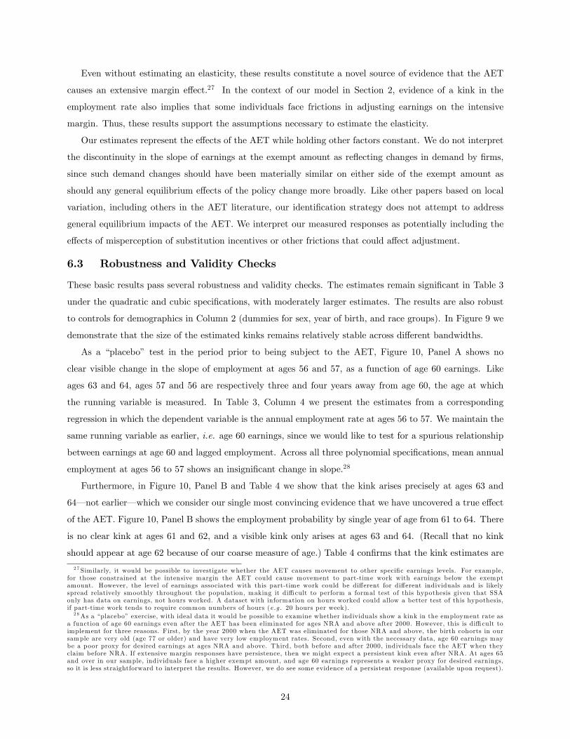
Even without estimating an elasticity, these results constitute a novel source of evidence that the AET

causes an extensive margin effect.27 In the context of our model in Section 2, evidence of a kink in the

employment rate also implies that some individuals face frictions in adjusting earnings on the intensive

margin. Thus, these results support the assumptions necessary to estimate the elasticity.

Our estimates represent the effects of the AET while holding other factors constant. We do not interpret

the discontinuity in the slope of earnings at the exempt amount as reflecting changes in demand by firms,

since such demand changes should have been materially similar on either side of the exempt amount as

should any general equilibrium effects of the policy change more broadly. Like other papers based on local

variation, including others in the AET literature, our identification strategy does not attempt to address

general equilibrium impacts of the AET. We interpret our measured responses as potentially including the

effects of misperception of substitution incentives or other frictions that could affect adjustment.

6.3 Robustness and Validity Checks

These basic results pass several robustness and validity checks. The estimates remain significant in Table 3

under the quadratic and cubic specifications, with moderately larger estimates. The results are also robust

to controls for demographics in Column 2 (dummies for sex, year of birth, and race groups). In Figure 9 we

demonstrate that the size of the estimated kinks remains relatively stable across different bandwidths.

As a “placebo” test in the period prior to being subject to the AET, Figure 10, Panel A shows no

clear visible change in the slope of employment at ages 56 and 57, as a function of age 60 earnings. Like

ages 63 and 64, ages 57 and 56 are respectively three and four years away from age 60, the age at which

the running variable is measured. In Table 3, Column 4 we present the estimates from a corresponding

regression in which the dependent variable is the annual employment rate at ages 56 to 57. We maintain the

same running variable as earlier, i.e. age 60 earnings, since we would like to test for a spurious relationship

between earnings at age 60 and lagged employment. Across all three polynomial specifications, mean annual

employment at ages 56 to 57 shows an insignificant change in slope.28

Furthermore, in Figure 10, Panel B and Table 4 we show that the kink arises precisely at ages 63 and

64– not earlier– which we consider our single most convincing evidence that we have uncovered a true effect

of the AET. Figure 10, Panel B shows the employment probability by single year of age from 61 to 64. There

is no clear kink at ages 61 and 62, and a visible kink only arises at ages 63 and 64. (Recall that no kink

should appear at age 62 because of our coarse measure of age.) Table 4 confirms that the kink estimates are

2 7 Similarly, it would be possible to investigate whether the AET causes movement to other specific earnings levels. For example,for those constrained at the intensive margin the AET could cause movement to part-time work with earnings below the exemptamount. However, the level of earnings associated with this part-time work could be different for different individuals and is likelyspread relatively smoothly throughout the population, making it diffi cult to perform a formal test of this hypothesis given that SSAonly has data on earnings, not hours worked. A dataset with information on hours worked could allow a better test of this hypothesis,if part-time work tends to require common numbers of hours (e.g. 20 hours per week).2 8As a “placebo” exercise, with ideal data it would be possible to examine whether individuals show a kink in the employment rate as

a function of age 60 earnings even after the AET has been eliminated for ages NRA and above after 2000. However, this is diffi cult toimplement for three reasons. First, by the year 2000 when the AET was eliminated for those NRA and above, the birth cohorts in oursample are very old (age 77 or older) and have very low employment rates. Second, even with the necessary data, age 60 earnings maybe a poor proxy for desired earnings at ages NRA and above. Third, both before and after 2000, individuals face the AET when theyclaim before NRA. If extensive margin responses have persistence, then we might expect a persistent kink even after NRA. At ages 65and over in our sample, individuals face a higher exempt amount, and age 60 earnings represents a weaker proxy for desired earnings,so it is less straightforward to interpret the results. However, we do see some evidence of a persistent response (available upon request).

24

insignificant at ages 61 and 62, but they are substantial and highly significant at ages 63 and 64. We are

particularly reassured by the small and insignificant kink at ages 61 and 62. This placebo check provides

further evidence that nonlinearities in the probability of employment (conditional on earnings at age 60) do

not drive our kink estimates. The absolute value of the kink grows substantially from age 63 to age 64, from

1.60 to 1.98, only a modest fraction of which can be explained by the higher fraction claiming at 64 (79.5

percent) than at 63 (74.5 percent). This is consistent with gradual adjustment to the AET, which Gelber,

Jones, and Sacks (2013) document at the intensive margin.

As another assessment of the validity of our approach, we conduct a permutation test in the spirit of

Ganong and Jäger (2015). In particular, we estimate a set of placebo changes in slope in the age 63 to 64

employment rate, using the same specification as our main estimates except that we examine the change in

slope at placebo locations of the exempt amount away from the true exempt amount. In Figure 11, we show

that the point estimate recovered from the actual exempt amount is located well below the distribution of

placebo estimates, reinforcing the view that we are detecting a true effect of the AET. This permutation test

shows a significant kink (p = 0.025).29 Following Landais (2015), we show in Figure 12 that the R-squared

of the regression in the baseline linear specification is maximized at the actual location of the kink, rather

than at placebo kink locations, again consistent with our finding a true effect of the AET.30

6.4 Estimating an Extensive Margin Elasticity

Our model allows us to go beyond documenting the effects of the AET by estimating an elasticity using

equation (9). In this equation we require an estimate of the average marginal tax rate; we use a marginal tax

rate incorporating the AET BRR as well as the average federal and state income and payroll marginal tax

rates, calculated using the TAXSIM calculator of the National Bureau of Economic Research and information

on individuals within the bandwidth distance from the kink in the Statistics of Income data in the years we

examine. Table 5 shows that the elasticity estimated using the full sample in the baseline linear specification

is 0.49. As discussed above, we interpret this as a lower bound on the elasticity. Since the lower bound is

large, our main conclusion is that the elasticity is large.

Separating the regressions by demographic group, the elasticity for women is 0.49, and the elasticity for

men is 0.25, consistent with the typical stylized fact that women have larger employment elasticities than

men.31 Whites and non-whites show similar employment elasticities, although the estimate is much more

precise in the larger white population. It is also of interest how the elasticity may vary depending on an

individual’s mean prior earnings, which we measure from ages 40 to 59. The elasticity point estimates are2 9Relative to our baseline specification, we also find similar, statistically significant results when we run our regressions using data at

the $50 bin mean level (or within bins of other sizes). This is an alternative way of demonstrating that the results are significant androbust to filtering out within-bin correlations; however, these results are superseded by the Ganong and Jäger permutation test resultsas the latter demonstrate that the kink is statistically unusual relative to the distribution of placebo estimates.3 0Recall that our running variable measures earnings relative to the exempt amount applying to OASI claimants when an individual

is age 60. Since the exempt amount is rising modestly over time (Figure 4), the exempt amount individuals face rises slightly from age60 to ages 63 and 64 when we measure employment. However, it rises by only $75.77 on average, far smaller than the bin size of $500that we use in our figures. Thus, our statistical and graphical results are similar to the baseline when we instead measure our runningvariable as age 60 earnings relative to the exempt amount that later applies to the same individual at ages 63 to 64.3 1Our study of women as well as men differs from the pre-2003 empirical literature on the employment effects of the AET cited above,

as well as Baker and Benjamin (1999) and Haider and Loughran (2008), all of which focus on studying only men. Gruber and Orszag(2003) find suggestive evidence of an impact among women but not among men.

25

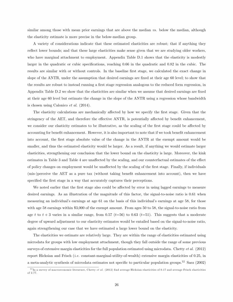
similar among those with mean prior earnings that are above the median vs. below the median, although

the elasticity estimate is more precise in the below-median group.

A variety of considerations indicate that these estimated elasticities are robust; that if anything they

reflect lower bounds; and that these large elasticities make sense given that we are studying older workers,

who have marginal attachment to employment. Appendix Table D.1 shows that the elasticity is modestly

larger in the quadratic or cubic specifications, reaching 0.66 in the quadratic and 0.82 in the cubic. The

results are similar with or without controls. In the baseline first stage, we calculated the exact change in

slope of the ANTR, under the assumption that desired earnings are fixed at their age 60 level; to show that

the results are robust to instead running a first stage regression analogous to the reduced form regression, in

Appendix Table D.2 we show that the elasticities are similar when we assume that desired earnings are fixed

at their age 60 level but estimate the change in the slope of the ANTR using a regression whose bandwidth

is chosen using Calonico et al. (2014).

The elasticity calculations are mechanically affected by how we specify the first stage. Given that the

stringency of the AET, and therefore the effective ANTR, is potentially affected by benefit enhancement,

we consider our elasticity estimates to be illustrative, as the scaling of the first stage could be affected by

accounting for benefit enhancement. However, it is also important to note that if we took benefit enhancement

into account, the first stage absolute value of the change in the ANTR at the exempt amount would be

smaller, and thus the estimated elasticity would be larger. As a result, if anything we would estimate larger

elasticities, strengthening our conclusion that the lower bound on the elasticity is large. Moreover, the kink

estimates in Table 3 and Table 4 are unaffected by the scaling, and our counterfactual estimates of the effect

of policy changes on employment would be unaffected by the scaling of the first stage. Finally, if individuals

(mis-)perceive the AET as a pure tax (without taking benefit enhancement into account), then we have

specified the first stage in a way that accurately captures their perceptions.

We noted earlier that the first stage also could be affected by error in using lagged earnings to measure

desired earnings. As an illustration of the magnitude of this factor, the signal-to-noise ratio is 0.61 when

measuring an individual’s earnings at age 61 on the basis of this individual’s earnings at age 58, for those

with age 58 earnings within $3,000 of the exempt amount. From ages 50 to 58, the signal-to-noise ratio from

age t to t + 3 varies in a similar range, from 0.57 (t=56) to 0.63 (t=51). This suggests that a moderate

degree of upward adjustment to our elasticity estimates would be entailed based on the signal-to-noise ratio,

again strengthening our case that we have estimated a large lower bound on the elasticity.

The elasticities we estimate are relatively large. They are within the range of elasticities estimated using

microdata for groups with low employment attachment, though they fall outside the range of some previous

surveys of extensive margin elasticities for the full population estimated using microdata. Chetty et al. (2012)

report Hicksian and Frisch (i.e. constant-marginal-utility-of-wealth) extensive margin elasticities of 0.25, in

a meta-analytic synthesis of microdata estimates not specific to particular population groups.32 Saez (2002)

3 2 In a survey of macroeconomic literature, Chetty et al. (2012) find average Hicksian elasticities of 0.17 and average Frisch elasticitiesof 2.77.

26

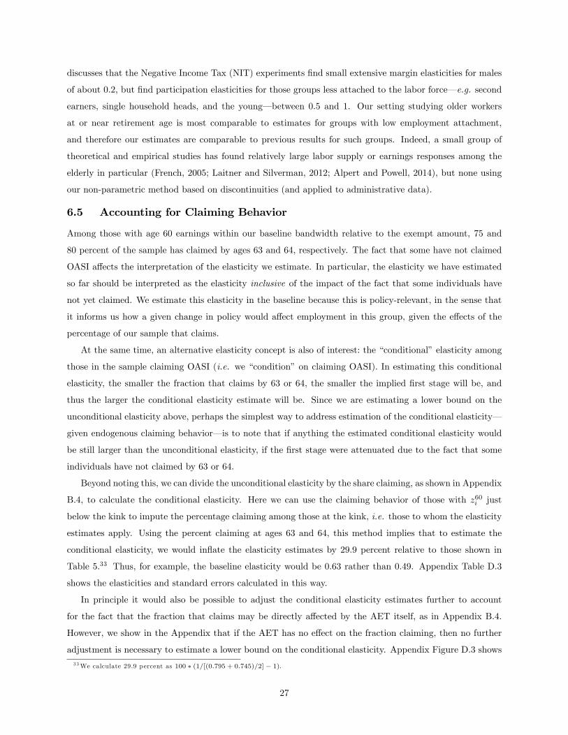
discusses that the Negative Income Tax (NIT) experiments find small extensive margin elasticities for males

of about 0.2, but find participation elasticities for those groups less attached to the labor force– e.g. second

earners, single household heads, and the young– between 0.5 and 1. Our setting studying older workers

at or near retirement age is most comparable to estimates for groups with low employment attachment,

and therefore our estimates are comparable to previous results for such groups. Indeed, a small group of

theoretical and empirical studies has found relatively large labor supply or earnings responses among the

elderly in particular (French, 2005; Laitner and Silverman, 2012; Alpert and Powell, 2014), but none using

our non-parametric method based on discontinuities (and applied to administrative data).

6.5 Accounting for Claiming Behavior

Among those with age 60 earnings within our baseline bandwidth relative to the exempt amount, 75 and

80 percent of the sample has claimed by ages 63 and 64, respectively. The fact that some have not claimed

OASI affects the interpretation of the elasticity we estimate. In particular, the elasticity we have estimated

so far should be interpreted as the elasticity inclusive of the impact of the fact that some individuals have

not yet claimed. We estimate this elasticity in the baseline because this is policy-relevant, in the sense that

it informs us how a given change in policy would affect employment in this group, given the effects of the

percentage of our sample that claims.

At the same time, an alternative elasticity concept is also of interest: the “conditional”elasticity among

those in the sample claiming OASI (i.e. we “condition”on claiming OASI). In estimating this conditional

elasticity, the smaller the fraction that claims by 63 or 64, the smaller the implied first stage will be, and

thus the larger the conditional elasticity estimate will be. Since we are estimating a lower bound on the

unconditional elasticity above, perhaps the simplest way to address estimation of the conditional elasticity–

given endogenous claiming behavior– is to note that if anything the estimated conditional elasticity would

be still larger than the unconditional elasticity, if the first stage were attenuated due to the fact that some

individuals have not claimed by 63 or 64.

Beyond noting this, we can divide the unconditional elasticity by the share claiming, as shown in Appendix

B.4, to calculate the conditional elasticity. Here we can use the claiming behavior of those with z60i just

below the kink to impute the percentage claiming among those at the kink, i.e. those to whom the elasticity

estimates apply. Using the percent claiming at ages 63 and 64, this method implies that to estimate the

conditional elasticity, we would inflate the elasticity estimates by 29.9 percent relative to those shown in

Table 5.33 Thus, for example, the baseline elasticity would be 0.63 rather than 0.49. Appendix Table D.3

shows the elasticities and standard errors calculated in this way.

In principle it would also be possible to adjust the conditional elasticity estimates further to account

for the fact that the fraction that claims may be directly affected by the AET itself, as in Appendix B.4.

However, we show in the Appendix that if the AET has no effect on the fraction claiming, then no further

adjustment is necessary to estimate a lower bound on the conditional elasticity. Appendix Figure D.3 shows3 3We calculate 29.9 percent as 100 ∗ (1/[(0.795 + 0.745)/2]− 1).

27

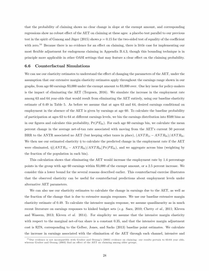
that the probability of claiming shows no clear change in slope at the exempt amount, and corresponding

regressions show no robust effect of the AET on claiming at these ages: a placebo test parallel to our previous

test in the spirit of Ganong and Jäger (2015) shows p = 0.15 for the two-sided test of equality of the coeffi cient

with zero.34 Because there is no evidence for an effect on claiming, there is little case for implementing our

most flexible adjustment for endogenous claiming in Appendix B.4.3, though this bounding technique is in

principle more applicable in other OASI settings that may feature a clear effect on the claiming probability.

6.6 Counterfactual Simulations

We can use our elasticity estimates to understand the effect of changing the parameters of the AET, under the

assumption that our extensive margin elasticity estimates apply throughout the earnings range shown in our

graphs, from age 60 earnings $3,000 under the exempt amount to $3,000 over. One key issue for policy-makers

is the impact of eliminating the AET (Tergesen, 2016). We simulate the increase in the employment rate

among 63 and 64 year-olds that would result from eliminating the AET entirely, using our baseline elasticity

estimate of 0.49 in Table 5. As before we assume that at ages 63 and 64, desired earnings conditional on

employment in the absence of the AET is given by earnings at age 60. To calculate the baseline probability

of participation at ages 63 to 64 at different earnings levels, we bin the earnings distribution into $500 bins as

in our figures and calculate this probability, Pr(PE0i). For each age 60 earnings bin, we calculate the mean

percent change in the average net-of-tax rate associated with moving from the AET’s current 50 percent

BRR to the ANTR associated no AET (but keeping other taxes in place), (ANTR1i −ANTR0i)/ANTR0i.

We then use our estimated elasticity η to calculate the predicted change in the employment rate if the AET

were eliminated, η[(ANTR1i − ANTR0i)/ANTR0i] Pr(PE0i), and we aggregate across bins (weighting by

the fraction of the population in each bin).

This calculation shows that eliminating the AET would increase the employment rate by 1.4 percentage

points in the group with age 60 earnings within $3,000 of the exempt amount, or a 2.5 percent increase. We

consider this a lower bound for the several reasons described earlier. This counterfactual exercise illustrates

that the observed elasticity can be useful for counterfactual predictions about employment levels under

alternative AET parameters.

We can also use our elasticity estimates to calculate the change in earnings due to the AET, as well as

the fraction of the change that is due to extensive margin responses. We use our baseline extensive margin

elasticity estimate of 0.49. To calculate the intensive margin response, we assume quasilinearity as in much

recent literature on earnings responses to kinked budget sets (e.g. Saez, 2010; Chetty et al., 2011; Kleven

and Waseem, 2013; Kleven et al. 2014). For simplicity we assume that the intensive margin elasticity

with respect to the marginal net-of-tax share is a constant 0.35, and that the intensive margin adjustment

cost is $278, corresponding to the Gelber, Jones, and Sacks (2013) baseline point estimates. We calculate

the increase in earnings associated with the elimination of the AET through each channel, intensive and

3 4Our evidence is not incompatible with Gruber and Orszag’s (2003) evidence on claiming: our results pertain to 63-64 year olds,whereas Gruber and Orszag (2003) find an effect of the AET on claiming among older groups.

28

extensive. For an individual i, the estimated total earnings response ∆Ei is:

∆Ei = Pr(PEno,i)zno,i − Pr(PEAET,i)zAET,i

= Pr(PEAET,i)(zno,i − zAET,i) + [Pr(PEno,i)− Pr(PEAET,i)]zno,i (15)

where Pr(PEAET ) and zAET are the probability of positive earnings under the AET and earnings under

the AET, respectively, and Pr(PEno) and zno refer to the levels of these variables once the AET has been

eliminated. The second line shows that the total response can be decomposed into an intensive margin

response (the first term) and an intensive margin response (the second term).

Our results show that in the group within $3,000 of the exempt amount, mean annual earnings at ages

63-64 (including zeroes) increase by 9.8 percent ($579) due to eliminating the AET, and 27.6 percent of the

increase in earnings is due to the extensive margin effect on the employment rate. Focusing only on the

intensive margin impact would overlook over one quarter of the total earnings response.

Our specific predictions are influenced by multiple factors: the elasticity is sizeable; the change in the

BRR due to eliminating the AET is large; but for those near the AET exempt amount that we study, the

change in the ANTR is relatively small. The elasticity could also be different at other points in the earnings

distribution, and moreover some individuals may tend to be unresponsive (e.g. those with zero earnings at

age 60) while others might be more responsive (e.g. those with age 60 earnings farther above the exempt

amount who experience a larger change in the ANTR, but not so far that the effect of the AET on the ANTR

greatly diminishes). Ultimately, our calculations do demonstrate that eliminating the AET can cause large

increases in earnings and employment, even using our lower bound point estimates.

7 Conclusion

We develop a method for estimating the extensive margin effect of non-linear taxes or transfers, relying

on empirically estimable quantities and a transparent RKD empirical design based on predictions from an

economic model that does not require parametric or distributional assumptions. Using this method, we show

that the AET has a large impact on extensive margin earnings decisions. Under our preferred specification,

the point estimate shows that the elasticity of the employment rate with respect to the ANTR is at least

0.49. We interpret this as a lower bound on the elasticity for several reasons. Estimating this large lower

bound is useful because it clearly distinguishes our study from previous literature largely finding that the

AET has little effect on employment.

This large response suggests that the AET can have important effects on the employment of older

workers. Our point estimates would imply that eliminating the AETwould increase the employment rate

among affected older workers by 1.4 percentage points (2.5 percent) in the group we study, and would

increase earnings by 9.8 percent. 27.6 percent of the aggregate earnings increase due to eliminating the AET

is associated with extensive margin decisions, demonstrating that focusing on intensive margin responses,

as in Saez (2010) and much other literature, can abstract from an important component of the earnings

29

impacts of tax and transfer programs. These estimates also suggest that the impact of eliminating the AET

on the budget is more positive than the budget-neutral estimates of the Congressional Budget Offi ce (2000),

which abstracted from extensive margin effects anywhere (including in the group around the kink we study).

Estimates of the full response to taxation must also capture responses that could move an individual from

above to below a convex kink, including moving to zero earnings. Indeed, our empirical approach could

be easily extended to estimate the effect of a kink on the probability of locating at any location or set of

locations below the kink (not only at zero earnings but also at positive earnings levels below the kink),

perhaps due to frictions like a limited earnings menu; if anything this would strengthen our conclusion that

the earnings losses due to the AET are large.

Our results are consistent with the hypothesis that some individuals are constrained from adjusting

on the intensive margin. The presence of frictions is consistent with recent literature including Chetty

(2012), Kleven and Waseem (2013), or Gelber, Jones, and Sacks (2013). It is also consistent with Abraham

and Houseman’s (2005) findings from a self-reported survey that suggest frictions among older workers in

particular, and Baker and Benjamin’s (1999) findings consistent with frictions in Canada. Our model points

out that as a result of these frictions, the observed extensive margin elasticity in our setting need not reflect

the structural elasticity, but the observed elasticity generally provides a lower bound.

Generally, in the context of the earnings decision, the estimation method requires: (1) a non-linear budget

set; (2) information on earnings or labor supply; and (3) a proxy for desired earnings on a linear budget set.

Thus, it appears that our method is applicable in many other contexts in which individuals make extensive

margin employment decisions, even outside of the AET, particularly because lagged earnings can proxy for

current desired earnings in a broad range of ages as we show. Although in our context we find large effects

of the marginal incentive to earn, our results do not imply that such effects are as large in all settings as

the literature suggests older individuals’ labor supply may be particularly elastic. It would be fruitful to

use our method to estimate employment elasticities in other contexts, including at other ages or in the

full age distribution. Future work could also attempt to investigate how to adjust elasticity estimates for

error in measuring desired earnings, whether through a context with a randomized experiment or through

assumptions that put additional structure on the measurement error. Though beyond the scope of this paper,

future research could also perform a welfare evaluation of the AET. Such an evaluation should also include

an assessment of the potential consumption smoothing benefits of the AET for older ages (Figinski and

Neumark, 2015). Future work could also further examine responses to kinks when individuals mis-perceive

their incentives. We are also currently investigating the mortality effect of the AET using a similar strategy.

Although we have modeled employment as a key first context, our method could be used to estimate the

elasticity of other extensive margin consumption decisions in the presence of non-linear pricing: the slope of

the extensive margin consumption decision should track the slope of the average price, inducing an estimable

kink in demand. Since non-linear pricing is found in many economic applications, our method should have

considerable scope to be adapted in other economic contexts.

30

ReferencesAaronson, S., Cajner, T., Fallick, B., Galbis-Reig, F., Smith, C., and Wascher, W. “LaborForce Participation: Recent Developments and Future Prospects,”Brookings Papers on Economic Activity,2014(2), 197-275.Abraham, K., and Houseman, S. (2005). “Work and Retirement Plans among Older Americans.”

In Reinventing the Retirement Paradigm, R. Clark and O. Mitchell, eds. Oxford, UK; New York: OxfordUniversity Press, 70-91.Abraham, K., and Kearney, M. (2017). “The Factors Behind the Decline in U.S. Employment Rates:

A Review of the Evidence.”University of Maryland Working Paper.Alpert, A., and Powell, D. (2014). “Estimating Intensive and Extensive Tax Responsiveness: Do

Older Workers Respond to Income Taxes.”RAND Working Paper.Altonji, J. G. and Paxson, C. H. (1988). “Labor Supply Preferences, Hours Constraints, and Hours-

Wage Trade-Offs,”Journal of Labor Economics, 6, 254-276.Brown, S.K, and Perron, R. (2011). “Assessing Current and Future Beneficiaries’Knowledge of

Social Security Benefits,”American Association of Retired Persons research report.Ando, M. (Forthcoming). “How Much Should We Trust Regression-Kink-Design Estimates?”Empirical

Economics.Baker, M., and Benjamin, D. (1999). “How do retirement tests affect the labor supply of older men?”

Journal of Public Economics, 71, 27-51.Battistin, E., and Chesher, A. (2014). “Treatment Effect Estimation with Covariate Measurement

Error.”Journal of Econometrics, 178(2), 707-715.Becker, G. (1976). “Altruism, Egoism, and Genetic Fitness: Economics and Sociobiology.”Journal of

Economic Literature, 14(3), 817-826.Bernheim, B. D., Fradkin, A., and Popov, I. (2015). “The Welfare Economics of Default Options

in 401(k) Plans,”American Economic Review, 105(9), 2798-2837.Bitler, M. P.,Gelbach, J. B., and Hoynes, H. W. (2006), “What Mean Impacts Miss: Distributional

Effects Of Welfare Reform Experiments,”American Economic Review, 96(4), 988-1012.Blinder, A. S., Gordon, R. H., and Wise, D. E. (1980). “Reconsidering the Work Disincentive

Effects of Social Security.”National Tax Journal, 33(4), 431-442.Blomquist, S., Kumar, A., Liang, C.-Y., and Newey, N. (2015). “Individual Heterogeneity,

Nonlinear Budget Sets, and Taxable Income.”Uppsala University Working Paper.Blundell, R., French, E. and Tetlow, G. (2016). “Retirement Incentives and Labor Supply.” In

Handbook of the Economics of Population Aging, John Piggott and Alan Woodland, eds., 457-566. Amster-dam: Elsevier.Blundell, R., and MaCurdy, T. (1999). “Labor Supply: A Review of Alternative Approaches.” In

Ashenfelter, O. and Card, D., eds., Handbook of Labor Economics 3A, 1560-1695. Amsterdam: Elsevier.Blundell, R. and Shephard, A. (2012). “Employment, Hours of Work and the Optimal Taxation of

Low-Income Families.”Review of Economic Studies, 79, 481-510.Brown, J., Kapteyn, A., Mitchell, O., and Mattox, T. (2013). “Framing the Social Security

Earnings Test.”Wharton Pension Research Council Working Paper.Burkhauser, R. V., and Turner, J. A. (1978). “A Time Series Analysis on Social Security and the

Market Work of Men at Younger Ages.” Journal of Political Economy, 86(4), 701-715.Burtless, G., and Hausman, J. A. (1978). “The Effect of Taxation on Labor Supply: Evaluating the

Gary Negative Income Tax Experiment.”Journal of Political Economy, 86(6), 1103-1130.Burtless, G., and Moffi tt, R. A. (1985). “The Joint Choice of Retirement Age and Postretirement

Hours of Work.” Journal of Labor Economics, 3, 209-236.Calonico, S., Cattaneo, M., and Titiunik, R. (2014). “Robust Nonparametric Confidence Intervals

for Regression-Discontinuity Designs.” Econometrica, 82(6), 2295-2326.Calonico, S., Cattaneo, M., Farrell, M. and Titiunik, R. (2016). “Regression Discontinuity

Designs Using Covariates.”University of Michigan Working Paper.Card, D., Lee, D., Pei, Z., and Weber, A. (2015). “Inference on Causal Effects in a Generalized

Regression Kink Design.”Econometrica, 83(6), 2463-2483.

31

Card, D., Johnston, A., Leung, P., Mas, A., and Pei, Z. (2016). “The Effect of UnemploymentBenefits on the Duration of Unemployment Insurance Receipt: New Evidence from a Regression Kink Designin Missouri, 2003-2013.”American Economic Review Papers and Proceedings, 105(5), 126-130.Chetty, R. (2012). “Bounds on Elasticities with Optimization Frictions.”Econometrica, 80(3), 969-1018.Chetty, R., Friedman, J. N., Olsen, T., and Pistaferri, L. (2011). “Adjustment Costs, Firm

Responses, and Micro vs. Macro Labor Supply Elasticities: Evidence from Danish Tax Records.”QuarterlyJournal of Economics, 126, 749-804.Chetty, R., Friedman, J. N., and Saez, E. (2013). “Using Differences in Knowledge Across Neigh-

borhoods to Uncover the Impacts of the EITC on Earnings.”American Economic Review, 103(7), 2683-2721.Chetty, R., Guren, A., Manoli, D., and Weber, A. (2012). “Does Indivisible Labor Explain the

Difference Between Mciro and Macro Elasticities? A Meta-Analysis of Extensive Margin Elasticities.” InAcemoglu, D., Parker, J., and Woodford, M., eds., NBER Macroeconomics Annual 2012 (Vol. 27, pp. 1-56).Chicago: University of Chicago Press.Chetty, R., Looney, A. and Kroft, K. (2007), “Salience and Taxation: Theory and Evidence.”

NBER Working Paper No. 13330.Christensen, K. (1990). “Bridges Over Troubled Water: How Older Workers View the Labor Market,”

in P. Doeringer, ed., Bridges to Retirement: Trends in the Labor Market for Older Workers (pp. 175-207).Ithaca, NY: ILR Press, Cornell University.Cogan, J. (1981). “Fixed Costs and Labor Supply.”Econometrica, 49, 945-963.Congressional Budget Offi ce. (2000). Pay-As-You-Go Estimate: H.R. 5, Senior Citizens’Freedom

to Work Act of 2000. Washington, D.C.: U.S. Government Printing Offi ce.Diamond, P. (1980). “Income Taxation with Fixed Hours of Work.” Journal of Public Economics,

13(1), 101-110.Diamond, P., and Gruber, J. (1999). “Social Security and Retirement in the United States.” In

Gruber, J. and Wise, D., eds., Social Security and Retirement around the World (pp. 437-473). Chicago:University of Chicago Press.Dickens, W., and Lundberg, S. (1993). “Labor Supply with Hours Restrictions.” International

Economic Review, 34(1), 169-192.Disney, R., and Smith, S. (2002). “The labour supply effect of the abolition of the earnings rule for

older workers in the United Kingdom.”Economic Journal, 112, C136-C152.Einav, L., Finkelstein, A., and Schrimpf, P. (2015). “The Response of Drug Expenditure to

Nonlinear Contract Design: Evidence from Medicare Part D.”Quarterly Journal of Economics, 130(2), 841-899.Eissa, N., and Hoynes, H. W. (2004). “Taxes and the Labor Market Participation of Married Couples:

the Earned Income Tax Credit.”Journal of Public Economics, 88(9-10), 1931-1958.Eissa, N., Kleven, H., and Kreiner, C. (2008). “Evaluation of four tax reforms in the United States:

Labor supply and welfare effects for single mothers.” Journal of Public Economics, 92(3-4), 795-816.Eissa, N., and Liebman, J. (1996). “Labor Supply Response to the Earned Income Tax Credit.”

Quarterly Journal of Economics, 111(2), 605-637.Engelhardt, G., and Kumar, A. (2014). “Taxes and the Labor Suplly of Older Americans: Recent

Evidence from the Social Security Earnings Test.”National Tax Journal, 67(2), 443-458.Figinski, T., and Neumark, D. (2015). "Does Eliminating the Earnings Test Increase the Incidence

of Low Income Among Older Women?" NBER Working Paper No. 21601.French, E. (2005). “The Effects of Health, Wealth, and Wages on Labour Supply and Retirement

Behaviour,”Review of Economic Studies, 72, 395-427.Friedberg, L. (1998). “The Social Security Earnings Test and Labor Supply of Older Men.” In Poterba,

J. M., ed., Tax Policy and the Economy (pp. 121-150). Chicago: University of Chicago Press.Friedberg, L. (2000). “The Labor Supply Effects of the Social Security Earnings Test.” Review of

Economics and Statistics, 82, 48-63.Friedberg, L., and Webb, A. (2009). “New Evidence on the Labor Supply Effects of the Social

Security Earnings Test.”In Brown, J.R., and Poterba, J. M., eds., Tax Policy and the Economy (pp. 1-35).Chicago: University of Chicago Press.Ganong, P., and Jäger, S. (2015). “A Permutation Test for the Regression Kink Design.”Harvard

University Working Paper.

32

Gelber, A., and Mitchell, J. (2012). “Taxes and Time Allocation: Evidence from Single Women andMen.” Review of Economic Studies, 79(3), 863-897.Gelber, A., Isen, A., and Song, J. (2016). “The Effect of Pension Income on Elderly Earnings:

Evidence from Social Security and Full Population Data.”UC Berkeley Working Paper.Gelber, A., Jones, D., and Sacks, D. (2013). “Earnings Adjustment Frictions: Evidence from the

Social Security Earnings Test.” NBER Working Paper No. 19491.Gelber, A., Jones, D., Sacks, D., and Song, J. (2017). “The Labor Force Participation Effects of

the Social Security Earnings Test.”Indiana University Working Paper.Gelber, A., Moore, T., and Strand, A. (Forthcoming). “The Effect of Disability Insurance Payments

on Beneficiaries’Earnings.”American Economic Journal: Economic Policy.Gruber, J., and Orzag, P. (2003). “Does the Social Security Earnings Test Affect Labor Supply and

Benefits Receipt.”National Tax Journal, 56, 755-773.Gruber, J., and Wise, D. (1999). “Introduction and Summary.” In Gruber, J., and Wise, D., eds.,

Social Security and Retirement Around the World (pp. 1-35). Chicago: University of Chicago Press.Gustman, A., and Steinmeier, T. (1985). “The 1983 Social Security Reforms and Labor Supply

Adjustment of Older Individuals in the Long Run.” Journal of Labor Economics, 3(2), 237-253.Gustman, A., and Steinmeier, T. (1991). “Changing the Social Security Rules for Work after 65.”

Industrial Labor and Relations Review, 44(4), 733-745.Haider, S., and Loughran, D. (2008). “The Effect of the Social Security Earnings Test on Male Labor

Supply: New Evidence from Survey and Administrative Data.” Journal of Human Resources, 43(1), 57-87.Hausman, J. (1981). “Labor Supply.” In Aaron, H. J. and Pechman, J. A., eds., How Taxes Affect

Economic Behavior (pp. 27-71). Washington, DC: Brookings Institution.Heckman, J. (1979). “Sample Selection Bias as a Specification Error.”Econometrica, 47(1), 153-161.Honig, M., and Reimers, C. (1989). “Is it Worth Eliminating the Retirement Test?” American

Economic Review, 79(2), 103-107.Hoynes, H. W. (1996). “Welfare Transfers in Two-Parent Families: Labor Supply and Welfare Partic-

ipation Under AFDC-UP.”Econometrica, 64, 295-332.Ito, K. (2014). “Do consumers respond to marginal or average price? Evidence from nonlinear electricity

pricing.”American Economic Review, 104(2), 537-563.J. K. Lasser Institute (1998). Your Income Tax: 1998. New York: Macmillan General Reference.Keane, M. P. (2011). “Labor Supply and Taxes: A Survey.” Journal of Economic Literature, 49(4),

961-1075.Keane, M. P. and Moffi tt, R. (1998). “A Structural Model of Multiple Welfare Program Participation

and Labor Supply.”International Economic Review, 39, 553-589.Kleven, H. (2016). “Bunching.”Annual Review of Economics, 8, 435-464.Kleven, H., and Kreiner, C. (2005). “Labor Supply Behavior and the Design of Tax and Transfer

Policy.”Danish Journal of Economics, 143, 321-358.Kleven, H., Landais, C., Saez, E., and Schultz, E. (2014). “Migration and Wage Effects of Taxing

Top Earners: Evidence from the Foreigners’Tax Scheme in Denmark.” Quarterly Journal of Economics,129(1), 333-378.Kleven, H. J., and Waseem, M. (2013). “Using Notches to Uncover Optimization Frcitions and

Structural Elasticities: Theory and Evidence from Pakistan.” Quarterly Journal of Economics, 128(2),669-723.Kline, P., and Tartari, M. (2016). “Bounding Labor Supply Responses to a Randomized Welfare

Experiment: A Revealed Preference Approach.”American Economic Review, 106, 972-1014.Kopczuk, W., and Munroe, D. (2015). “Mansion Tax: The effect of Transfer Taxes on the Residential

Real Estate Market.”American Economic Journal: Economic Policy, 7(2), 214-257.Kopczuk, W., Saez, E., and Song, J. (2010). “Earnings Inequality and Mobility in the United

States: Evidence from Social Security Data since 1937.”Quarterly Journal of Economics,125(1), 91-128.Laitner, J., and Silverman, D. (2012). “Consumption, Retirement, and Social Security: Evaluating

the Effi ciency of Reform that Encourages Longer Careers.”Journal of Public Economics, 96, 615-634.Landais, C. (2015). “Assessing the Welfare Effects of Unemployment Benefits Using the Regression

Kink Design.”American Economic Journal: Economic Policy, 7(4), 243-278.

33

Leonesio, M. V. (1990). “The Effects of the Social Security Earnings Test on the Labor-Market Activityof Older Americans: A Review of Empirical Evidence.” Social Security Bulletin, 53(5), 2-21.Liebman, J., and Luttmer, E. (2015). “Would People Behave Differently If They Better Understood

Social Security? Evidence From a Field Experiment.”American Economic Journal: Economic Policy, 7(1),275-99.Liebman, J., and Zeckhauser, R. (2004). “Schmeduling.”Harvard University working paper.Manoli, D., and Weber, A. (2016). “The Effects of the Early Retirement Age on Retirement Deci-

sions.”NBER Working Paper 22561.Manoli, D., and Weber, A. (Forthcoming). “Nonparametric Evidence on the Effects of Financial

Incentives on Retirement Decisions.”American Economic Journal: Economic Policy.Manski, C. (2014). “Identification of Income-Leisure Preferences and Evaluation of Income Tax Policy,”

Quantitative Economics, 5, 145-174.McCrary, J. (2008). “Manipulation of the Running Variable in the Regression Discontinuity Design: A

Density Test.”Journal of Econometrics, 142(2), 698-714.McDonald, J. F., and Moffi tt, R. A. (1980). “The Uses of Tobit Analysis.”Review of Economics

and Statistics, 62(2), 318-321.Meyer, B. D., and Rosenbaum, D. T. (2001). “Welfare, the Earned Income Tax Credit, and the

Labor Supply of Single Mothers.”Quarterly Journal of Economics, 116(3), 1063-1114.Moffi tt, R. (1983). “An Economic Model of Welfare Stigma.” American Economic Review, 73(5),

1023-1035.Nielson, H. S., Sorenson, T., and Taber, C. (2010). “Estimating the Effect of Student Aid on

College Enrollment from a Government Grant Policy Reform.” American Economic Journal: EconomicPolicy, 2(2), 185-215.Powell, J. L. (1994). “Estimation of Semiparametric Models.”In Engle, R. F., and McFadden, D., eds.,

Handbook of Econometrics (pp. 2443-2521). Amsterdam: Elsevier.Rubin, D. B. (1974). “Estimating Causal Effects of Treatments in Randomized and Nonrandomized

Studies.”Journal of Educational Psychology, 66.5, 688-701.Saez, E. (2002). “Optimal Income Transfer Programs: Intensive versus Extensive Labor Supply Re-

sponses.”Quarterly Journal of Economics, 117(3), 1039-1073.Saez, E. (2010). “Do Taxpayers Bunch at Kink Points?”American Economic Journal: Economic Policy,

2, 180-212.Saez, E., Slemrod, J. and Giertz, S. (2012). “The Elasticity of Taxable Income with Respect to

Marginal Tax Rates: A Critical Review.”Journal of Economic Literature, 50(1), 3-50.Social Security Administration. (2012). Social Security Handbook. Washington, D.C.: SSA.Song, J. G. (2004). “Evaluating the Initial Impact of Eliminating the Retirement Earnings Test.” Social

Security Bulletin, 65(1), 1-15.Song, J. G., and Manchester, J. (2007). “New Evidence on Earnings and Benefit Claims Following

Changes in the Retirement Earnings Test.”Journal of Public Economics, 91, 669-700.Tergesen, A. (2016). “How to Get People to Delay Retirement.”Wall St. Journal, March 21.Turner, L. (2014). “The Road to Pell is Paved with Good Intentions: The Economic Incidence of

Federal Student Grant Aid.” University of Maryland Working Paper.Utendorf, K. (2001/2002). “The Upper Part of the Earnings Distribution in the United States: How

Has It Changed?”Social Security Bulletin, 64 (3), 1-11.Viscusi, K. (1979). Welfare of the Elderly: An Economic Analysis and Policy Prescription. New York,

NY: John Wiley and Sons.Vroman, W. (1985). “Some Economic Effects of the Retirement Test.” In Ehrenberg, R., ed., Research

in Labor Economics (Vol. 7, pp. 31-89). Greenwich, CT: Jai Press, Inc.

34

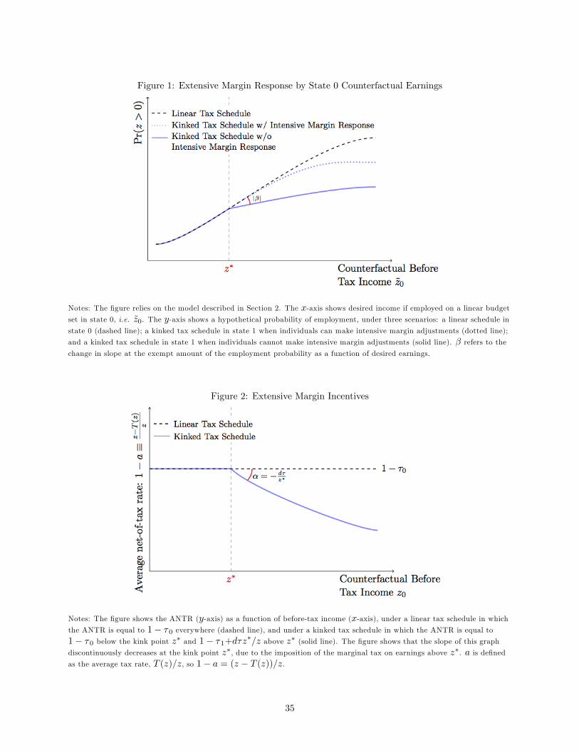
Figure 1: Extensive Margin Response by State 0 Counterfactual Earnings

Notes: The figure relies on the model described in Section 2. The x-axis shows desired income if employed on a linear budgetset in state 0, i.e. z0. The y-axis shows a hypothetical probability of employment, under three scenarios: a linear schedule instate 0 (dashed line); a kinked tax schedule in state 1 when individuals can make intensive margin adjustments (dotted line);

and a kinked tax schedule in state 1 when individuals cannot make intensive margin adjustments (solid line). β refers to thechange in slope at the exempt amount of the employment probability as a function of desired earnings.

Figure 2: Extensive Margin Incentives

Notes: The figure shows the ANTR (y-axis) as a function of before-tax income (x-axis), under a linear tax schedule in whichthe ANTR is equal to 1− τ0 everywhere (dashed line), and under a kinked tax schedule in which the ANTR is equal to

1− τ0 below the kink point z∗ and 1− τ1+dτz∗/z above z∗ (solid line). The figure shows that the slope of this graph

discontinuously decreases at the kink point z∗, due to the imposition of the marginal tax on earnings above z∗. a is definedas the average tax rate, T (z)/z, so 1− a = (z − T (z))/z.

35

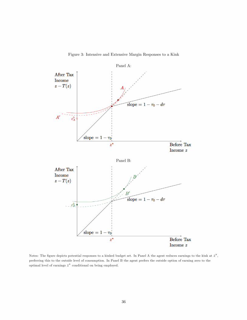
Figure 3: Intensive and Extensive Margin Responses to a Kink

Panel A:

Panel B:

Notes: The figure depicts potential responses to a kinked budget set. In Panel A the agent reduces earnings to the kink at z∗,preferring this to the outside level of consumption. In Panel B the agent prefers the outside option of earning zero to the

optimal level of earnings z∗ conditional on being employed.

36

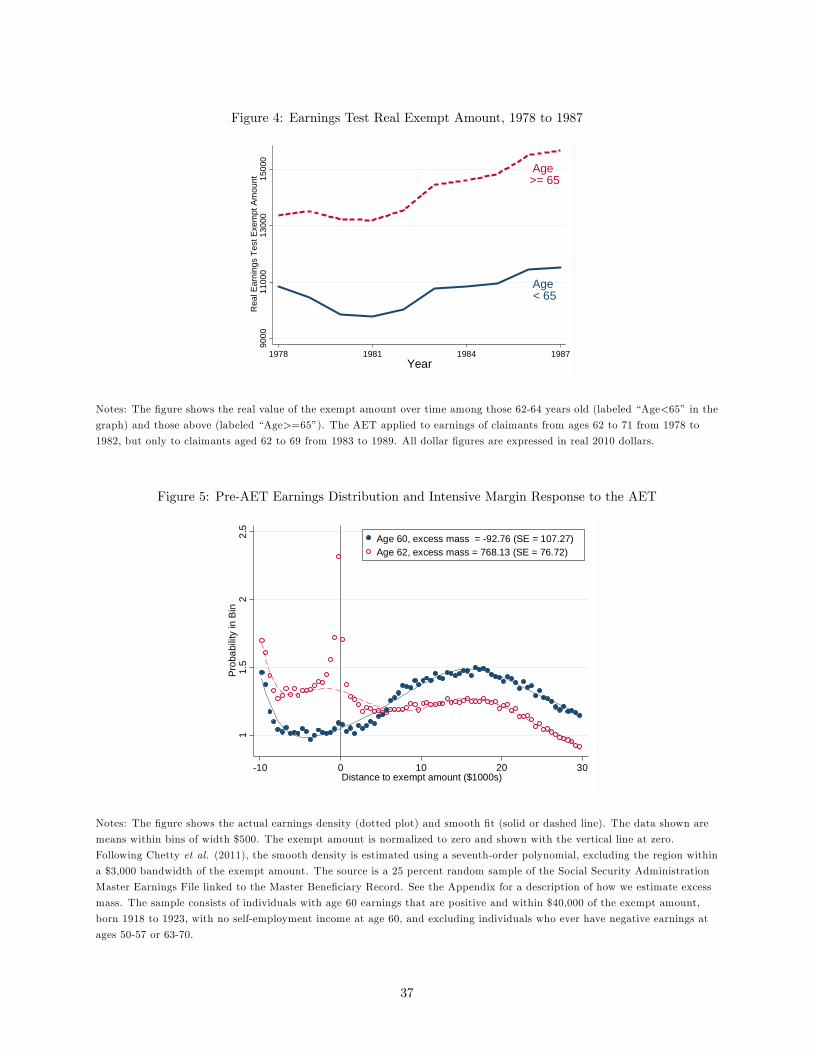
Figure 4: Earnings Test Real Exempt Amount, 1978 to 1987

Age< 65

Age>= 65

9000

1100

013

000

1500

0R

eal E

arni

ngs 

Test

 Exe

mpt

 Am

ount

1978 1981 1984 1987Year

Notes: The figure shows the real value of the exempt amount over time among those 62-64 years old (labeled “Age<65” in the

graph) and those above (labeled “Age>=65”). The AET applied to earnings of claimants from ages 62 to 71 from 1978 to

1982, but only to claimants aged 62 to 69 from 1983 to 1989. All dollar figures are expressed in real 2010 dollars.

Figure 5: Pre-AET Earnings Distribution and Intensive Margin Response to the AET

11.

52

2.5

Pro

babi

lity 

in B

in

­10 0 10 20 30Distance to exempt amount ($1000s)

Age 60, excess mass  = ­92.76 (SE = 107.27)Age 62, excess mass = 768.13 (SE = 76.72)

Notes: The figure shows the actual earnings density (dotted plot) and smooth fit (solid or dashed line). The data shown are

means within bins of width $500. The exempt amount is normalized to zero and shown with the vertical line at zero.

Following Chetty et al. (2011), the smooth density is estimated using a seventh-order polynomial, excluding the region within

a $3,000 bandwidth of the exempt amount. The source is a 25 percent random sample of the Social Security Administration

Master Earnings File linked to the Master Beneficiary Record. See the Appendix for a description of how we estimate excess

mass. The sample consists of individuals with age 60 earnings that are positive and within $40,000 of the exempt amount,

born 1918 to 1923, with no self-employment income at age 60, and excluding individuals who ever have negative earnings at

ages 50-57 or 63-70.

37

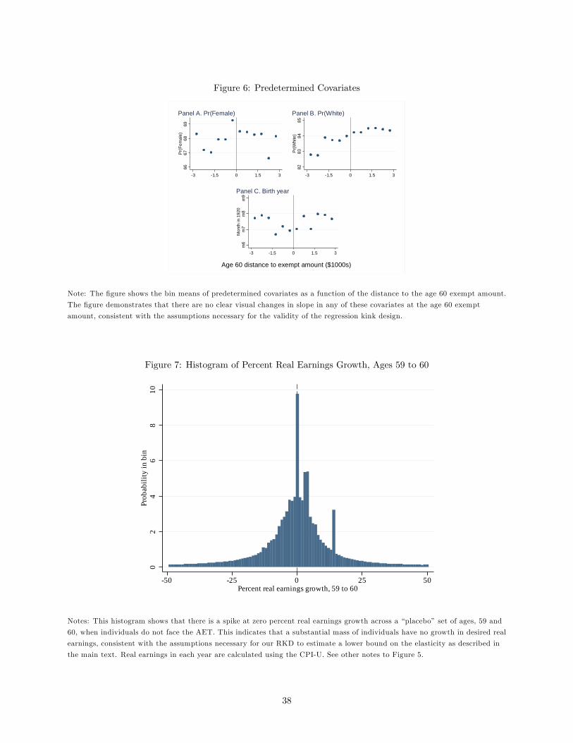
Figure 6: Predetermined Covariates

6667

6869

Pr(

Fem

ale)

­3 ­1.5 0 1.5 3

Panel A. Pr(Female)

8283

8485

Pr(

Whi

te)

­3 ­1.5 0 1.5 3

Panel B. Pr(White)

m6

m7

m8

m9

Mon

th in

 192

0

­3 ­1.5 0 1.5 3

Panel C. Birth year

Age 60 distance to exempt amount ($1000s)

Note: The figure shows the bin means of predetermined covariates as a function of the distance to the age 60 exempt amount.

The figure demonstrates that there are no clear visual changes in slope in any of these covariates at the age 60 exempt

amount, consistent with the assumptions necessary for the validity of the regression kink design.

Figure 7: Histogram of Percent Real Earnings Growth, Ages 59 to 60

02

46

810

Prob

abili

ty in

 bin

­50 ­25 0 25 50Percent real earnings growth, 59 to 60

Notes: This histogram shows that there is a spike at zero percent real earnings growth across a “placebo” set of ages, 59 and

60, when individuals do not face the AET. This indicates that a substantial mass of individuals have no growth in desired real

earnings, consistent with the assumptions necessary for our RKD to estimate a lower bound on the elasticity as described in

the main text. Real earnings in each year are calculated using the CPI-U. See other notes to Figure 5.

38

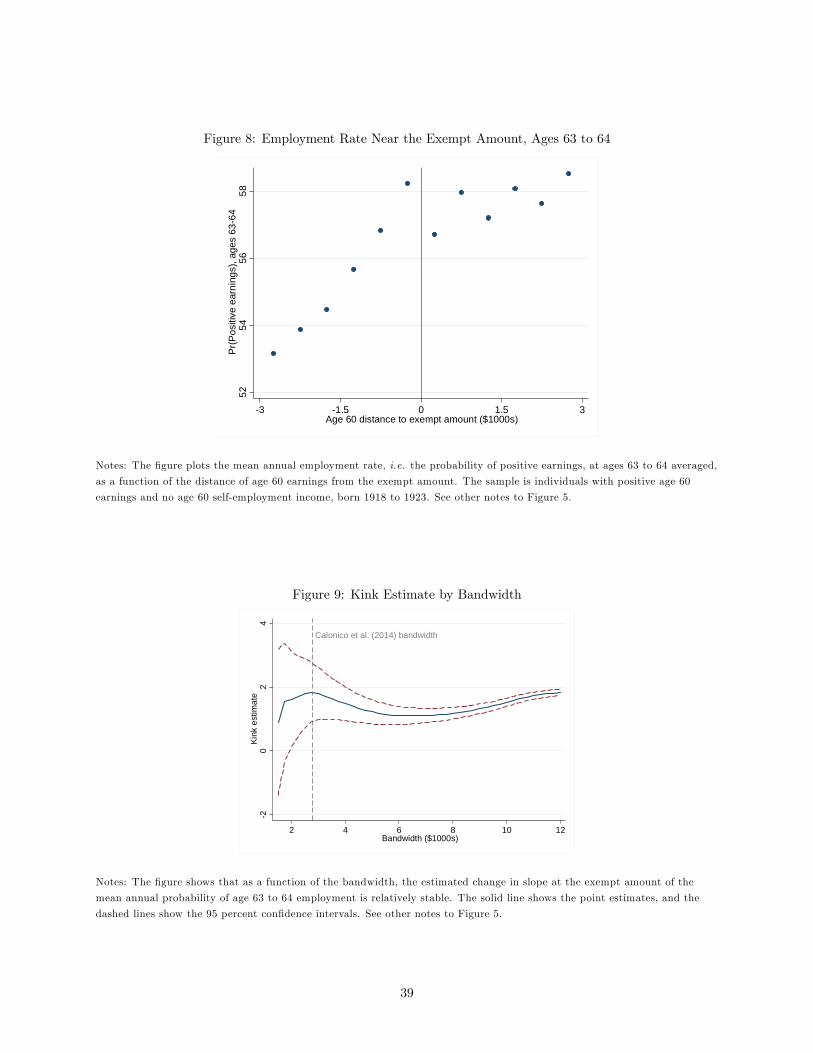
Figure 8: Employment Rate Near the Exempt Amount, Ages 63 to 64

5254

5658

Pr(

Pos

itive

 ear

ning

s), a

ges 

63­6

4

­3 ­1.5 0 1.5 3Age 60 distance to exempt amount ($1000s)

Notes: The figure plots the mean annual employment rate, i.e. the probability of positive earnings, at ages 63 to 64 averaged,

as a function of the distance of age 60 earnings from the exempt amount. The sample is individuals with positive age 60

earnings and no age 60 self-employment income, born 1918 to 1923. See other notes to Figure 5.

Figure 9: Kink Estimate by Bandwidth

Calonico et al. (2014) bandwidth

­20

24

Kin

k es

timat

e

2 4 6 8 10 12Bandwidth ($1000s)

Notes: The figure shows that as a function of the bandwidth, the estimated change in slope at the exempt amount of the

mean annual probability of age 63 to 64 employment is relatively stable. The solid line shows the point estimates, and the

dashed lines show the 95 percent confidence intervals. See other notes to Figure 5.

39

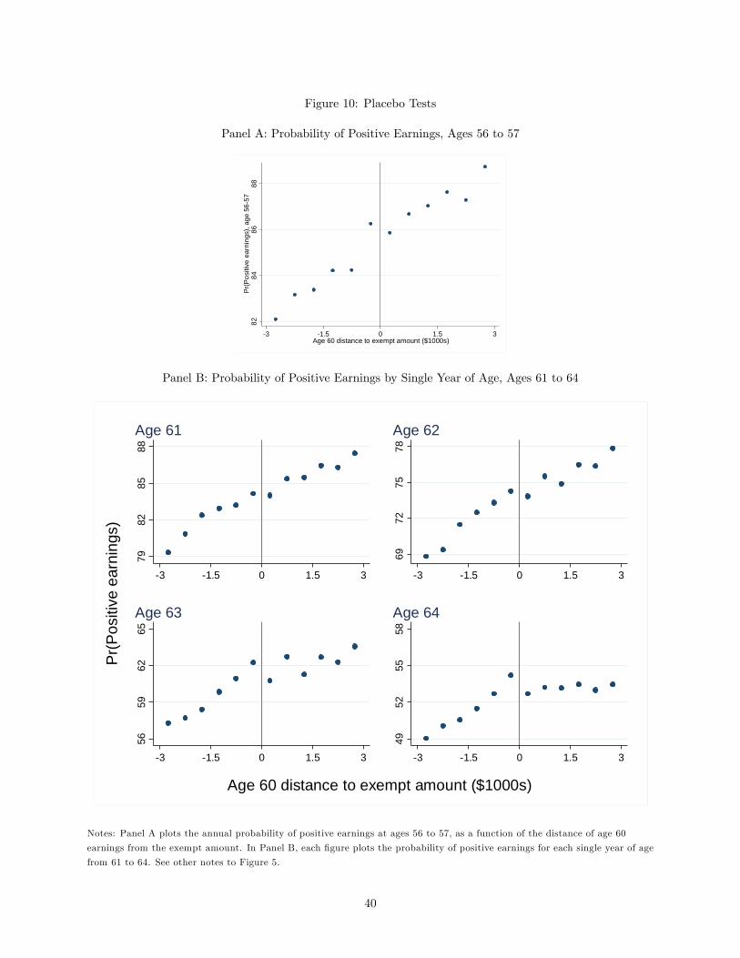
Figure 10: Placebo Tests

Panel A: Probability of Positive Earnings, Ages 56 to 57

8284

8688

Pr(P

ositi

ve e

arni

ngs)

, age

 56­

57

­3 ­1.5 0 1.5 3Age 60 distance to exempt amount ($1000s)

Panel B: Probability of Positive Earnings by Single Year of Age, Ages 61 to 64

7982

8588

­3 ­1.5 0 1.5 3

Age 61

6972

7578

­3 ­1.5 0 1.5 3

Age 62

5659

6265

­3 ­1.5 0 1.5 3

Age 63

4952

5558

­3 ­1.5 0 1.5 3

Age 64

Pr(

Pos

itive

 ear

ning

s)

Age 60 distance to exempt amount ($1000s)

Notes: Panel A plots the annual probability of positive earnings at ages 56 to 57, as a function of the distance of age 60

earnings from the exempt amount. In Panel B, each figure plots the probability of positive earnings for each single year of age

from 61 to 64. See other notes to Figure 5.

40

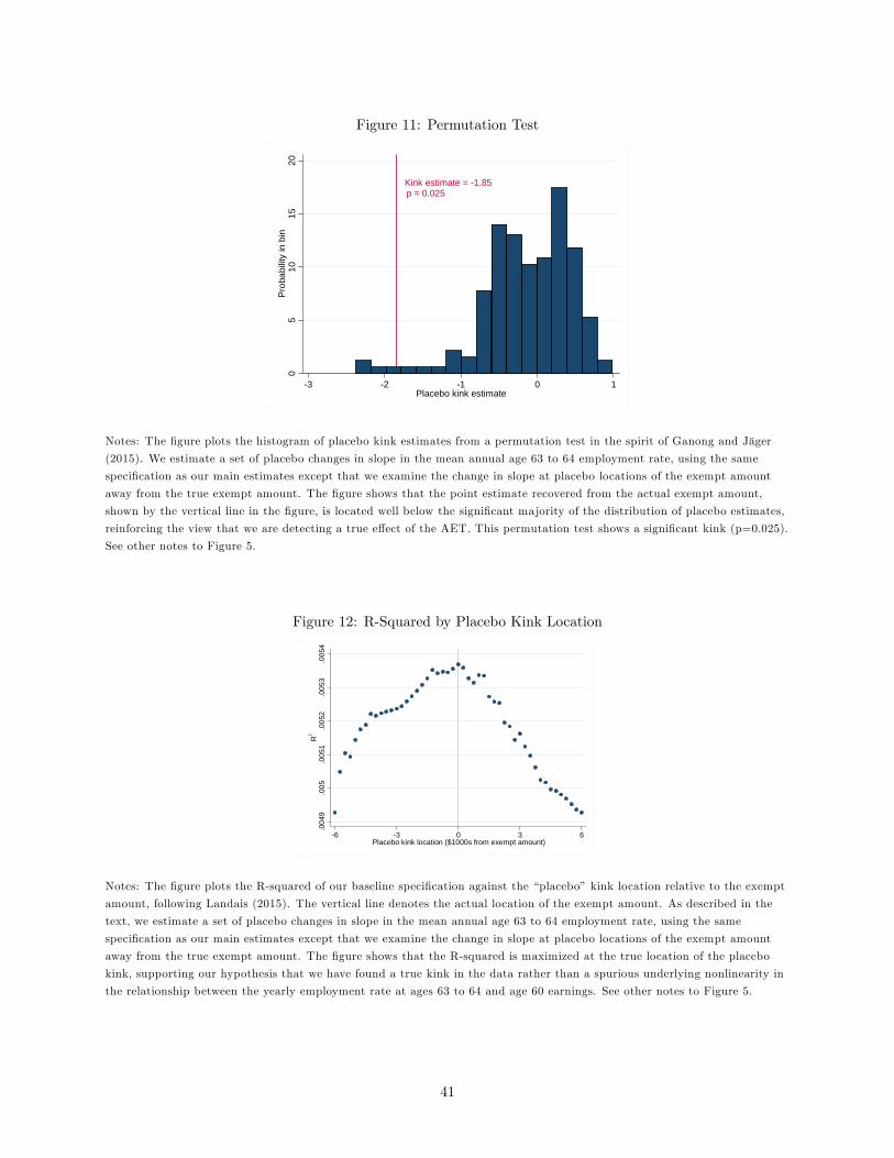
Figure 11: Permutation Test

Kink estimate = ­1.85 p = 0.025

05

1015

20P

roba

bilit

y in

 bin

­3 ­2 ­1 0 1Placebo kink estimate

Notes: The figure plots the histogram of placebo kink estimates from a permutation test in the spirit of Ganong and Jäger

(2015). We estimate a set of placebo changes in slope in the mean annual age 63 to 64 employment rate, using the same

specification as our main estimates except that we examine the change in slope at placebo locations of the exempt amount

away from the true exempt amount. The figure shows that the point estimate recovered from the actual exempt amount,

shown by the vertical line in the figure, is located well below the significant majority of the distribution of placebo estimates,

reinforcing the view that we are detecting a true effect of the AET. This permutation test shows a significant kink (p=0.025).

See other notes to Figure 5.

Figure 12: R-Squared by Placebo Kink Location

.004

9.0

05.0

051

.005

2.0

053

.005

4R

2

­6 ­3 0 3 6Placebo kink location ($1000s from exempt amount)

Notes: The figure plots the R-squared of our baseline specification against the “placebo”kink location relative to the exempt

amount, following Landais (2015). The vertical line denotes the actual location of the exempt amount. As described in the

text, we estimate a set of placebo changes in slope in the mean annual age 63 to 64 employment rate, using the same

specification as our main estimates except that we examine the change in slope at placebo locations of the exempt amount

away from the true exempt amount. The figure shows that the R-squared is maximized at the true location of the placebo

kink, supporting our hypothesis that we have found a true kink in the data rather than a spurious underlying nonlinearity in

the relationship between the yearly employment rate at ages 63 to 64 and age 60 earnings. See other notes to Figure 5.

41

Table 1: Summary Statistics(1) (2)

Within $2,797 of Full EarningsExempt Amount Range

Percent of years with positive 56.53 63.27earnings, ages 63 to 64 (45.92) (44.05)Annual earnings, ages 63 to 64 $5,813 $20,115(including zeroes) ($8,134) ($24,599)Claim age (if claimed) 63.13 63.68

(2.61) (2.14)Percent female 68.00 41.85

(46.65) (49.33)Percent white 83.96 89.30

(36.70) (30.91)Year of birth 1920.62 1920.52

(1.68) (1.69)N 95,960 1,425,600

Notes: The table shows the means of each variable shown in the row headings, with the standard deviation in parentheses,

from a 25 percent random sample of the Social Security Administration Master Earnings File and Master Beneficiary Record.

The sample is all individuals born 1918-1923 with positive earnings at age 60, and satisfying the other sample restrictions

described in the main text. In Column 1, the bandwidth relative to the AET exempt amount, $2,797, corresponds to the

bandwidth used in our main regressions. For comparison, Column 2 shows individuals from the full range of earnings.

Earnings are in thousands of real 2010 dollars. N’s refer to the number of individuals.

Table 2: Initial Tests of Smoothness(1) (2) (3) (4)

Estimated KinkWhite Female Year of

Density (Indicator) (Indicator) BirthLinear -0.057 -0.0005 -0.035 0.052

(0.067) (0.36) (0.34) (0.018)***N 141,110 172,383 330,556 102,640Quadratic -0.26 -0.074 0.0069 0.074

(0.36) (1.48) (0.28) (0.017)***N 141,110 696,139 348,920 304,306Cubic -0.26 -0.98 -2.25 0.038

(0.36) (0.69) (0.72)*** (0.028)N 141,110 282,460 362,174 308,690

Notes: The table presents tests for the smoothness of the earnings density, and of three pre-determined covariates (indicators

for being white or female, and year of birth). The table reports coeffi cients corresponding to β1 in equation (13), reflecting

the change in slope in the outcome at the age 60 exempt amount, as a function of age 60 earnings relative to the exempt

amount. The column headings indicate the outcome variable, while the row headings indicate the specification of the running

variable (linear, quadratic, or cubic). The number of individuals N in each regression is shown below the standard error. In

Columns 2 to 4, robust standard errors following Calonico et al. (2014) are reported in parentheses, and the bandwidth is also

chosen using Calonico et al. (2014). The resulting difference in bandwidths is the reason for the discrepancy across

specifications in the number of individuals included in these regressions. The N’s are the same across the specifications for the

density outcome in Column 1 because following previous literature, we use the McCrary (2008) procedure to calculate the

bandwidth, bin size, and standard error for the density outcome. Here and in the following tables, *** indicates p<0.01; **

indicates p<0.05; and * indicates p<0.10, all from two-tailed tests of equality with zero. See other notes to Table 1.

42

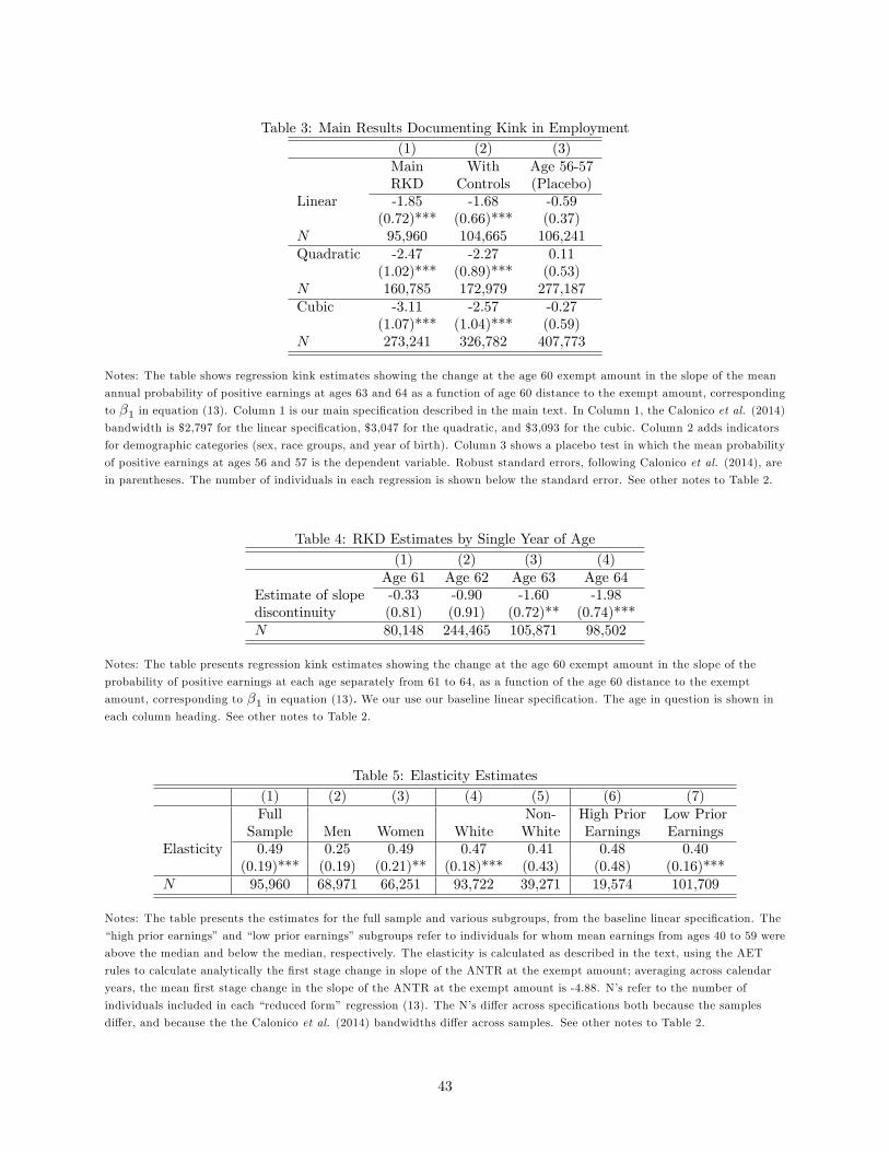
Table 3: Main Results Documenting Kink in Employment(1) (2) (3)Main With Age 56-57RKD Controls (Placebo)

Linear -1.85 -1.68 -0.59(0.72)*** (0.66)*** (0.37)

N 95,960 104,665 106,241Quadratic -2.47 -2.27 0.11

(1.02)*** (0.89)*** (0.53)N 160,785 172,979 277,187Cubic -3.11 -2.57 -0.27

(1.07)*** (1.04)*** (0.59)N 273,241 326,782 407,773

Notes: The table shows regression kink estimates showing the change at the age 60 exempt amount in the slope of the mean

annual probability of positive earnings at ages 63 and 64 as a function of age 60 distance to the exempt amount, corresponding

to β1 in equation (13). Column 1 is our main specification described in the main text. In Column 1, the Calonico et al. (2014)

bandwidth is $2,797 for the linear specification, $3,047 for the quadratic, and $3,093 for the cubic. Column 2 adds indicators

for demographic categories (sex, race groups, and year of birth). Column 3 shows a placebo test in which the mean probability

of positive earnings at ages 56 and 57 is the dependent variable. Robust standard errors, following Calonico et al. (2014), are

in parentheses. The number of individuals in each regression is shown below the standard error. See other notes to Table 2.

Table 4: RKD Estimates by Single Year of Age(1) (2) (3) (4)

Age 61 Age 62 Age 63 Age 64Estimate of slope -0.33 -0.90 -1.60 -1.98discontinuity (0.81) (0.91) (0.72)** (0.74)***N 80,148 244,465 105,871 98,502

Notes: The table presents regression kink estimates showing the change at the age 60 exempt amount in the slope of the

probability of positive earnings at each age separately from 61 to 64, as a function of the age 60 distance to the exempt

amount, corresponding to β1 in equation (13). We our use our baseline linear specification. The age in question is shown ineach column heading. See other notes to Table 2.

Table 5: Elasticity Estimates(1) (2) (3) (4) (5) (6) (7)Full Non- High Prior Low PriorSample Men Women White White Earnings Earnings

Elasticity 0.49 0.25 0.49 0.47 0.41 0.48 0.40(0.19)*** (0.19) (0.21)** (0.18)*** (0.43) (0.48) (0.16)***

N 95,960 68,971 66,251 93,722 39,271 19,574 101,709

Notes: The table presents the estimates for the full sample and various subgroups, from the baseline linear specification. The

“high prior earnings”and “low prior earnings”subgroups refer to individuals for whom mean earnings from ages 40 to 59 were

above the median and below the median, respectively. The elasticity is calculated as described in the text, using the AET

rules to calculate analytically the first stage change in slope of the ANTR at the exempt amount; averaging across calendar

years, the mean first stage change in the slope of the ANTR at the exempt amount is -4.88. N’s refer to the number of

individuals included in each “reduced form” regression (13). The N’s differ across specifications both because the samples

differ, and because the the Calonico et al. (2014) bandwidths differ across samples. See other notes to Table 2.

43

Appendix: For Online Publication

A Proofs of Propositions and Other ClaimsProposition 1: In general the slope of dPr( zn1>0|zn0)

dzn0will be given by:

dPr (zn1 > 0| zn0)

dzn0= g (qn1|n)

dqn,1dzn0

+∂G (qn1|n)

∂n

dn

dzn0(A.1)

Focusing on the first term in the expression for dPr (zn1 > 0| zn0) /dzn0 in (A.1), we have:

dqn,1dzn0

=∂v (zn1 − T1 (zn1) , zn1;n)

∂zn1

dzn1

dzn0+∂v (zn1 − T1 (zn1) , zn1;n)

∂n

dn

dzn0

=∂v (zn1 − T1 (zn1) , zn1;n)

∂n

dn

dzn0(A.2)

When agents are unrestricted in their intensive margin earnings choice, we can set the first term on the rightside of (A.2) to zero. For those with zn0 < z∗ or zn0 > z∗ + ∆z∗, ∂v (zn1 − T1 (zn1) , zn1;n) /∂zn1 = 0 dueto the envelope theorem.35 For those with z∗ ≤ zn0 ≤ z∗ + ∆z∗, we have dzn1/dzn0 = 0, since zn1 = z∗

for everyone in this set– i.e. these agents bunch at z∗. Substituting for dqn1/dzn0 in (A.1) using (A.2), wehave:

dPr (zn1 > 0| zn0)

dzn0= g (qn1|n)

∂v (zn1 − T1 (zn1) , zn1;n)

∂n

dn

dzn0+∂G (qn1|n)

∂n

dn

dzn0(A.3)

when individuals are able to adjust on both the intensive and extensive margins.

Our smoothness assumptions imply that this slope is continuous, and in particular it is continuous at z∗

since n, qn1, zn1, T1 (·) and ∂G ( qnj |n) /∂n are all continuous in zn0 at z∗. Furthermore, g (·) and ∂v/∂nare likewise continuous in their arguments. Thus, we have:

limzn0→z∗+

dPr (zn1 > 0| zn0)

dzn0− limzn0→z∗−

dPr (zn1 > 0| zn0)

dzn0= 0 (A.4)

That is, the employment probability does not exhibit any first-order change in slope at z∗, even though theANTR does feature such a discontinuity.

Proposition 2: If zn1 ≡ zn0, the general expression for dPr (zn1 > 0| zn0) /dzn0 from (A.1) still holds.However, we now have a slightly different expression for the critical level of fixed costs, which is now eval-uated at zn0, implying qn1 ≡ v (zn0 − T1 (zn0) , zn0;n)− v0. Accordingly, we have a different expression fordqn1/dzn0 relative to (A.2). Since zn1 = zn0 for everyone, we have:

dqn1

dzn0=∂v (zn0 − T1 (zn0) , zn0;n)

∂zn0+∂v (zn0 − T1 (zn0) , zn0;n)

∂n

dn

dzn0(A.5)

where the key difference is that ∂v/∂z and ∂v/∂n are evaluated at zn0 instead of zn1. For those withzn0 < z∗, since T1 (·) = T0 (·) and zn1 = zn0, it is still the case that ∂v (zn0 − T1 (zn0) , zn0;n) /∂zn0 = 0 dueto the envelope theorem. However, the first term in (A.5) for those with zn0 > z∗ is now:

∂v (zn0 − T1 (zn0) , zn0;n)

∂zn0= (1− τ1) vc + vz

= λn

[(1− τ1) +

vzvc

](A.6)

where λn ≡ vc, and vc and vz are the partial derivatives of v (·) with respect to c and z, respectively,evaluated at (zn0 − T1 (zn0) , zn0;n).35 In this and other similar expressions elsewhere we evaluate the partial derivative of v with respect to z allowing both

earnings and consumption to change via the budget constraint, but holding n constant.

44

Thus, we now have:

dPr (zn1 > 0| zn0)

dzn0=

{g (qn1|n) ∂v(zn0−T1(zn0),zn0;n)

∂ndndzn0

+ ∂G( qn1|n)∂n

dndzn0

, if zn0 < z∗

g (qn1|n)[λn

[(1− τ1) + vz

vc

]+ ∂v(zn0−T1(zn0),zn0;n)

∂ndndzn0

]+ ∂G( qn1|n)

∂ndndzn0

, if zn0 ≥ z∗

(A.7)Note also that:

limzn0→z∗+

vz (zn0 − T1 (zn0) , zn0;n)

vc (zn0 − T1 (zn0) , zn0;n)= − (1− τ0) (A.8)

where we have used the first order condition for zn,0 and the fact that limzn0→z∗

T1 (zn0) = T0 (z∗). We now

have the following expression for the difference in slopes at z∗:

limzn0→z∗+

dPr (zn1 > 0| zn0)

dzn0− limzn0→z∗−

dPr (zn1 > 0| zn0)

dzn0= lim

zn0→z∗+g (qn1|n) · λn

[(1− τ1) +

vzvc

]= g (qn∗1|n∗) · λn∗ [(1− τ1)− (1− τ0)]

= −dτ · λn∗ · g (qn∗1|n∗) (A.9)

where qn∗1, n∗, and λn∗ all refer the individual for whom zn0 = z∗.

Estimation of Kink with Measurement Error: In Section 4.2, we argue that in the case of measurementerror, i.e. π (z0, vit) < 1, we estimate a lower bound on our elasticity. Here we formally demonstratethis result. Recall that our relationship between earnings at age 60 and desired earnings at ages 63-64 isz60 = z0it + pitvit. We assume that the joint distribution of (p, v), conditional on z60, is continuous andcontinuously differentiable in z60 at z60 = z∗. Consider the estimated kink in employment, as a function ofearnings at age 60, i.e. the numerator in equation (12), using z60 as the running variable. Denote this asβRKD:

βRKD ≡ limz60i →z∗+

∂ Pr(Lit = 1| z60

i

)∂z60i

− limz60i →z∗−

∂ Pr(Lit = 1| z60

i

)∂z60i

Let the potential deviation in desired earnings, v, have a distribution with the CDF M (v| z) and pdfm (v| z), conditional on z60 = z. We have the following:

βRKD =

∫π (z∗, v)

[lim

z60i →z∗+

∂ Pr(Lit = 1| z60

i

)∂z60i

− limz60i →z∗−

∂ Pr(Lit = 1| z60

i

)∂z60i

]m (v| z∗)

+

∫(1− π (z∗ − v, v))

[lim

z60i →z∗+

∂ Pr(Lit = 1| z60

i

)∂z60i

− limz60i →z∗−

∂ Pr(Lit = 1| z60

i

)∂z60i

]m (v| z∗)

=

∫π (z∗, v)

[lim

zi0t→z∗+∂ Pr (Lit = 1| zi0t)

∂zi0t− limz60i →z∗−

∂ Pr (Lit = 1| zi0t)∂zi0t

]m (v| z∗)

+

∫(1− π (z∗ − v, v))

[lim

zi0t→z∗+−vit

∂ Pr (Lit = 1| zi0t)∂zi0t

− limzi0t→z∗−−vit

∂ Pr (Lit = 1| zi0t)∂zi0t

]m (v| z∗)

= π · β (z∗) + (1− π)

∫1− π (z∗ − v, v)

1− π β (z∗ − v)m (v| z∗)

where

π =

∫π (z∗, v)m (v| z∗)

β (z) = limzi0t→z

∂ Pr (Lit = 1| zi0t)∂zi0t

− limzi0t→z

∂ Pr (Lit = 1| zi0t)∂zi0t

That is, π is the probability that pit = 0 among individuals with z60i = z∗ and β (z) is a the kink in

employment at z that would estimated if desired earnings, zi0t, were observed.

45

Given our assumptions on smoothness in heterogeneity and assuming the only relevant kink in the taxschedule is at z∗, we have:

β (z) =

{β if z = z∗

0 if z 6= z∗

Here β is the kink in employment among those who face a kink, as defined in equation (9). Thus, we have:

βRKD = π · β

It follows that if π (z, v) < 1, i.e. we have measurement error in desired earnings when using z60 as a proxy,then we estimate a lower bound on our elasticity when using the formula in equation (9). In other words,the estimated kink among those with age 60 earnings near z∗ reflects a weighted average of the subset ofindividuals who will actually face the kink at ages 63-64 and the subset who will not. Furthermore, whenπ (z, v) = 0, i.e. there is no persistence in earnings from age 60 to ages 63-64, we expect no employmentkink. Note, we only require that the distribution of v be smooth as a function of z60. Thus, we can allowfor cases where v is not mean zero, e.g. where there is a systematic change in mean desired earnings fromage 60 to ages 63-64. Note as well that we can relax the assumption that the only kink in the tax scheduleis at z∗ and can instead assume that the set of other possible kinks is of measaure zero.

B Model ExtensionsB.1 Extension to Two or More Discrete Job ChoicesWe begin by focusing on two key options within the menu of positive earnings: one at the interior optimumin state 0, zn0, and another “next-best” job at an alternative level of earnings, znbn . This allows for anarbitrary number (whether finite or infinite) of discrete choices that are less preferred than the “next-best”job. The model can also be easily extended to allow for the possibility that multiple earnings levels give thesame “next best”utility level as znbn .

Let vnbn be the utility level associated with the next-best level of earnings:

vnbn ≡ v(znbn − T

(znbn), znbn ;n

)(B.10)

As it is possible that the kink lowers utility at zn0 while leaving utility at znbn unaffected, the probability ofworking in state 1 is one minus the probability that non-employment is preferred to both the earnings levelzn0 and the earnings level znbn of the next-best job:

Pr (zn1 > 0| zn0) = 1− Pr(v0 ≥ vnbn − qn1 and v0 ≥ v (zn0 − T1 (zn0) , zn0;n)− qn1

)= 1− Pr

(v0 ≥ vnbn − qn1

∣∣ qn1 < qn1

)· Pr (qn1 < qn1)

= 1− Pr(v0 ≥ vnbn − qn1

∣∣ qn1 < qn1

)· [1−G ( qn1|n)] (B.11)

The slope of the employment function is now a more complex expression:

dPr (zn1 > 0|zn0)

dzn0= −

dPr(v0 ≥ vnbn − qn1|qn1 < qn1

)dzn0

[1−G (qn1|n)]

+ Pr(v0 ≥ vnbn − qn1

∣∣ qn1 < qn1

)·[dG (qn1|n)

dzn0

](B.12)

We now explore under what conditions this slope reduces to that of our earlier model in Section 2.4, inwhich intensive margin earnings in state 1 are constrained at their state 0 level. We will show in generalthat this is true for those with state 0 earnings below z∗. Next, we show that for those with state 0 earningsjust above z∗, the slope is likewise unaffected relative to the model in Section 2.4, as long as the next-bestjob offers a level of earnings that is discretely different than the new interior optimum z∗.

Consider individuals earning below z∗ in state 0. We first focus on the term Pr(v0 ≥ vnbn − qn1|qn1 < qn1

).

46

We can show the following for the agents in this set for whom qn1 < qn1:

v0 > v (zn0 − T1 (zn0) , zn0;n)− qn1

= v (zn0 − T0 (zn0) , zn0;n)− qn1

> vnbn − qn1 (B.13)

where in the first line we used the fact that qn1 < qn1 and the definition of qn1. In the second line weused the fact that T1 (zn0) = T0 (zn0) for individuals with zn0 < z∗. In the third line we used the fact thatv (zn0 − T0 (zn0) , zn0;n) ≥ vnbn due to revealed preference in state 0. It follows that:

Pr(v0 ≥ vnbn − qn1

∣∣ qn1 < qn1, zn0 < z∗)

= 1

⇒dPr

(v0 ≥ vnbn − qn1

∣∣ qn1 < qn1, zn0 < z∗)

dzn0= 0 (B.14)

In other words, if an individual with state 0 earnings below z∗ prefers the outside option in the absence ofthe next-best job, she would continue to prefer it in the presence of the next-best job.

Using the results in (B.14), we can simplify the expression in (B.12), for those with zn0 < z∗:

dPr (zn1 > 0| zn0)

dzn0=

dG (qn1|n)

dzn0

= g (qn1|n)∂v (zn0 − T1 (zn0) , zn0;n)

∂n

dn

dzn0+∂G (qn1|n)

∂n

dn

dzn0(B.15)

where the second line follows from equation (A.7). Thus, the presence of a menu of discrete options does notaffect the results for those with zn0 < z∗. Intuitively, after the introduction of a kink, the individual’s state0 optimal earnings amount zn0 is still available and is the only positive earnings level relevant for extensivemargin decisions.

Now consider individuals with zn0 ≥ z∗ and recall that we are ultimately interested in the change inslope of the employment rate at z∗. Any change in the slope of the employment function at z∗ will dependon the following limit:

limzn0→z∗+

dPr (zn1 > 0| zn0)

dzn0=

[− limzn0→z∗+

dPr(v0 ≥ vnbn − qn1

∣∣ qn1 < qn1

)dzn0

][1−G (qn∗1|n∗)]

+

[lim

zn0→z∗+Pr(v0 ≥ vnbn − qn1

∣∣ qn1 < qn1)

](dG(qn∗1|n∗)

dzn0

)(B.16)

Note the following:

limzn0→z∗+

Pr(v0 ≥ vnbn − qn1

∣∣ qn1 < qn1

)= lim

zn0→z∗+Pr(v0 ≥ vnbn − qn1

∣∣ v0 ≥ v (zn0 − T1 (zn0) , zn0;n)− qn1

)= Pr

(v0 ≥ vnbn∗ − qn∗1

∣∣ v0 ≥ v (z∗ − T0 (z∗) , z∗;n∗)− qn∗1)

= 1 (B.17)

In the second line, we used the fact that limzn0→z∗

zn0 = z∗ and T1 (z∗) = T0 (z∗) , and the final line follows

from revealed preference: z∗ was initially chosen over the next-best job.

We require that in the neighborhood of z∗ the earnings level offered at the next-best job be discretelydifferent than that of the state 0 job; thus, we assume that:

limzn0→z∗

znbn 6= z∗ (B.18)

This assumption rules out alternative jobs that can be made arbitrarily close to the level of state 0 earnings.Intuitively, if this were not so then individuals earning just above z∗ in state 0 would be able to replicate

47

intensive margin adjustment, which we have shown smooths out any kink in the employment function thatwould otherwise exist.

The assumption in (B.18) implies that the limit in (B.17) is reached at some level of state 0 earningsstrictly above z∗. That is, as we approach z∗ from above, the probability that preferring the outside optionwithout an alternative job implies preferring it in the presence of the next-best job plateaus at 1 at somepoint before reaching z∗. Thus, we have:

limzn0→z∗+

dPr(v0 ≥ vnbn − qn1

∣∣ qn1 < qn1

)dzn0

= 0 (B.19)

As before, (B.17) and (B.19) can be used to simplify (B.16) as follows:

limzn0→z∗+

dPr (zn1 > 0|zn0)

dzn0= lim

zn0→z∗+dG (qn1|n)

dzn0

= g (qn∗1|n∗)[−dτ · λn∗ +

∂v (zn∗0 − T1 (zn∗0) , zn∗0;n∗)

∂n

dn

dzn0

]+dG (qn∗1|n∗)

dn

dn

dzn0(B.20)

where the second line follows from equation (A.7). Combining (B.20) and (B.15), we have the same resultas equation (8) of Section 2.4, i.e. our earlier model with zn1 = zn0. Note that this result features as aspecial case the scenario in which the agent has the choice among a full-time job at zn0, a part-time job assome lower level of earnings, or not working. Furthermore, this result can be extended beyond a setting withmultiple, discrete earnings options to allow for some continuity in the choice set, as long as the options allstrictly differ from z∗ among those with state 0 earnings near z∗.

B.2 Estimating the Structural Elasticity among Constrained Types, π∗BIn the model presented in Section 2.6, we may wish to estimate the structural elasticity among constrainedtypes, η∗B . We may be able to use data on extensive margin responses between states 0 and 1 along withevidence on intensive margin responses in state 1 to perform this decomposition; however, to do so we willrequire more restrictive assumptions on the underlying primitives. For notational convenience, define the setR = {n| z∗ < zn,0 < z∗ +4z∗} as the set of individuals in state 0 with earnings in the range that bunchesunder a kink in the absence of intensive margin frictions. Define NR,0 as the number of individuals in thisrange in state 0. As before, denote Type A earners as those who can adjust on the intensive margin andType B earners as those who cannot, in state 1. Define NRA,0 and NRB,0 as the number of Type A andType B earners in the set R, respectively. It follows that:

NR,0 = NRA,0 +NRB,0

Similarly, define NR,1 as the number of individuals in the set R that are still employed in state 1. That is{n| z∗ < zn,0 < z∗ +4z∗, zn,1 > 0}. Again, define NRA,1 and NRB,1 as the number of Type A and Type Bearners in the set R that are also employed in state 1. Again, we have:

NR,1 = NRA,1 +NRB,1

Finally, define NBunch as the number of individuals in the set R that bunch in state 1. Note that:

NBunch = NRA,1

We can show the following:

Pr (zn,1 > 0| z∗ < zn,0 < z∗ +4z∗) = Pr (zn,1 > 0|n ∈ R)

= (1− π∗B) Pr (zn,1 > 0|n ∈ R,A)

+π∗B Pr (zn,1 > 0|n ∈ R,B)

48

Define N0 as the total number of people in the labor force in state 0 and define N1 as the number of thesepeople also in the labor force in state 1. If we define B as the share of all such earners bunching in state 1,then we have:

B =NBunchN1

=NRA,1N1

=NRA,1NRA,0

NRA,0NR,0

NR,0N0

N0

N1

=Pr (zn,1 > 0|n ∈ R,A) (1− π∗B)× Pr (z∗ < zn,0 < z∗ +4z∗)

Pr (zn,1 > 0| zn,0 > 0)

In addition, if we assume that Type A and Type B individuals have the same preferences and differ onlyin the ability to adjust to z∗, then the only difference in employment exit between the two groups is due tothe lack of intensive margin adjustment on the part of the Type B agents. In this case, we can show thefollowing:

Pr (zn,1 > 0|n ∈ R,B) =

∫ z∗+4z∗

z∗

dPr (zn,1 > 0| zn,0 = ζ,B)

dzn,0h0 (ζ) dζ

=

∫ z∗+4z∗

z∗

[dPr (zn,1 > 0| zn,0 = ζ,A)

dzn,0+ λn

[(1− τ1) +

vzvc

]g ( qn,1|n)

]h0 (ζ) dζ

= Pr (zn,1 > 0|n ∈ R,A) +

∫ z∗+4z∗

z∗

[λn

[(1− τ1) +

vzvc

]g ( qn,1|n)

]h0 (ζ) dζ,

where the second line follows from equation (A.7). We will use a first-order approximation, assuming

λn

[(1− τ1) + vz

vc

]g ( qn,1|n) is constant in the set R. Then we have:

∫ z∗+4z∗

z∗

[λn

[(1− τ1) +

vzvc

]g ( qn,1|n)

]h0 (ζ) dζ ≈ −dτ · λn∗ · g ( qn∗,1|n = n∗)

∫ z∗+4z∗

z∗h0 (ζ) dζ

=βRKD

π∗B· Pr (z∗ < zn,0 < z∗ +4z∗)

Generally, λn and vz/vc are decreasing over this range. If g ( qn,1|n) is also weakly decreasing, then we willbe overstating the difference between Pr (zn,1 > 0|n ∈ R,B) and Pr (zn,1 > 0|n ∈ R,A).

Now, consider estimating the following:

limzn,0↓z∗

dE [ 1− T1 (zn,1) /zn,1| zn,0, zn,1 > 0]

dzn,0− limzn,0↑z∗

dE [ 1− T1 (zn,1) /zn,1| zn,0, zn,1 > 0]

dzn,0

which is the difference at the exempt amount z∗ in the slope of the average net-of-tax rate in state 1, asa function of state 0 earnings, among the set of individuals who do not exit employment between states 0and 1. Note that since Type A individuals bunch, the average tax rate is constant for this group. Thus, thedifference in the slope will be zero for this group. For the Type B individuals, the difference will be:[

d (1− T1 (z) /z)

dz− d (1− T0 (z) /z)

dz

]∣∣∣∣z=z∗

= −T′

1 (z∗)

z∗+T1 (z∗)

(z∗)2 +

T ′0 (z∗)

z∗− T0 (z∗)

(z∗)2

= −T′

1 (z∗)− T ′0 (z∗)

z∗

= −dτz∗

49

As a result, the average in the difference in slopes for the total group will be:

βATR =NRA,1NR,1

· 0 +NRB,1NR,1

·(−dτz∗

)=

NR,0NR,1

NRB,0NR,0

NRB,1NRB,0

·(−dτz∗

)=

Pr (zn,1 > 0|n ∈ R,B)π∗BPr (zn,1 > 0| z∗ < zn,0 < z∗ +4z∗)

(−dτz∗

)

We thus have four equations:

Pr (zn,1 > 0| z∗ < zn,0 < z∗ +4z∗) = (1− π∗B) Pr (zn,1 > 0|n ∈ R,A) + π∗B Pr (zn,1 > 0|n ∈ R,B)

B =Pr (zn,1 > 0|n ∈ R,A) (1− π∗B)× Pr (z∗ < zn,0 < z∗ +4z∗)

Pr (zn,1 > 0| zn,0 > 0)

βRKD =Pr (zn,1 > 0|n ∈ R,B)− Pr (zn,1 > 0|n ∈ R,A)

Pr (z∗ < zn,0 < z∗ +4z∗) /π∗B

βATR =Pr (zn,1 > 0|n ∈ R,B)π∗B

Pr (zn,1 > 0| z∗ < zn,0 < z∗ +4z∗)

(−dτz∗

)and four unknowns: 4z∗, π∗B , Pr (zn,1 > 0|n ∈ R,A) and Pr (zn,1 > 0|n ∈ R,B). We do not have a closedform solutions for either Pr (zn,1 > 0| z∗ < zn,0 < z∗ +4z∗) or Pr (z∗ < zn,0 < z∗ +4z∗).

However, if we estimate a flexible polynomial for the employment rate and for the density in state 0, wecan numerically solve for π∗B . This can be combined with η to recover η

∗B . However, this requires additional

assumptions relative to our non-parametric estimate of the observed elasticity, which is a non-parametriclower bound on the structural elasticity; for example, as noted above, to recover η∗B we would need to assumethat types A and B have identical preferences.

B.3 Fully Dynamic Extension of the ModelIn this section we briefly demonstrate under what conditions our results continue to hold once our modelis extended to a multi-period setting with forward-looking agents. We again have two states of the world,state 0 and state 1. In this multi-period model, the tax schedule is the same across the two states forperiods 1, . . . , t − 1. However, in period t, the tax schedule is linear in state 0 and has a convex kink atz∗ in state 1. The tax schedules are once again the same across the two states during periods t + 1, . . . , T .(For simplicity we assume here that the tax schedules across the two states are once again the same duringperiods t + 1, . . . , T , but the model can be easily extended to assume that in each of these periods the taxschedule is linear in state 0 and has a kink at z∗ in state 1.)

We assume that preferences and the economic environment yield a dynamic programming problem asfollows. In each period, individuals maximize:

ut (cnjt, znjt;n) = v (cnjt, znjt;n)− qnjt · 1 {znjt > 0}+ Vt (Anjt, znjt;n) (B.21)

subject to a dynamic budget constraint:

cnjt = (1 + rt−1)Anj,t−1 + znjt − Tj (znjt)−Anjt (B.22)

where Anjt is the level of assets at the end of period t. The value function for the next period, Vt (·), maydepend on the level of assets passed forward and potentially the level of earnings in the current period. Forexample, working today may have some effect on the choice set in the next period.

50

We once again index individuals by their counterfactual earnings in period t in state 0, and we focus onthe probability of having positive earnings in period t in state 1, conditional on the counterfactual earningslevel in state 0: Pr (zn1t > 0| zn0t). In addition to the assumptions we have made above in Section 2.3, weassume that the value function Vt (·) is C1 in A, z, and n. Agents choose c, z, and A to maximize utility.The outside value of not working in period t, v0 (Anj,t−1), depends on the current level of assets and includesthe continuation value of future periods. Finally, the distribution of fixed costs of working, G (q|n, t), nowdepends on the time period as well.

The first-order conditions when earnings are positive are now:

vz + Vz = −λ (1− T ′ (z))vc = VA = λ (B.23)

where λ is the marginal utility of wealth. Using these conditions, we can show that there will still be bunchingin response to a kink among those who can adjust on the intensive margin. As before, individuals will workif the utility conditional on working exceeds that of not working:

v (cnjt, znjt;n) + Vt

(Anjt, znjt;n

)− v0 (Anj,t−1)− qnjt > 0 (B.24)

where the “∼”denotes optimal levels conditional on working. The probability of working in period 1 is still:

Pr (zn1t > 0| zn0t) = G (qn1t|n, t) (B.25)

where now:

qn1t ≡ v (cn1t, zn1t;n) + Vt

(An1t, zn1t;n

)− v0 (An1,t−1) (B.26)

We now show under what conditions our main results still hold in this dynamic setting. First, the slopeof the employment rate will still be:

dPr (zn1t > 0| zn0t)

dzn0t= g (qn1t|n, t)

dqn1t

dzn0t+dG (qn1t|n, t)

dn

dn

dzn0t(B.27)

We will have a new expression for the first term on the right of equation (B.27). After substituting for cn1t

in (B.26) using the dynamic budget constraint in (B.22) we have:

dqn1t

dzn0t=

∂v(

(1 + rt−1) An1,t−1 + zn1t − T1 (zn1t)− An1t, zn1t;n)

∂zn1t+∂Vt

(An1t, zn1t;n

)∂zn1t

dzn1t

dzn0t

+

∂v(

(1 + rt−1) An1,t−1 + zn1t − T1 (zn1t)− An1t, zn1t;n)

∂An1t

+∂Vt

(An1t, zn1t;n

)∂An1t

dAn1t

dzn0t

+

∂v(

(1 + rt−1) An1,t−1 + zn1t − T1 (zn1t)− An1t, zn1t;n)

∂n+∂Vt

(An1t, zn1t;n

)∂n

dn

dzn0t

+

∂v(

(1 + rt−1) An1,t−1 + zn1t − T1 (zn1t)− An1t, zn1t;n)

∂An1,t−1

−∂v0

(An1,t−1

)∂An1,t−1

dAn1,t−1

dzn0t

= [(1− T ′1 (z)) vc + vz + Vz]dzn1t

dzn0t+ [−vc + VA]

dAn1t

dzn0t+ [vn + Vn]

dn

dzn0t+[(1 + rt−1) vc − v0

A

] dAn1,t−1

dzn0t

(B.28)

For those with zn0t < z∗ or zn0t > z∗+ ∆z∗, we can use the first-order conditions in (B.23) to show that thefirst term in (B.28) equals zero when agents are able to adjust on the intensive margin as in Section 2.3. For

51

those with z∗ ≤ zn0t ≤ z∗ + ∆z∗, the first term in (B.28) equals zero: dzn1t/dzn0t = 0 since zn1t = z∗ foreveryone in this latter set due to bunching. Additionally, the second term in (B.28) equals zero for everyone,due to the first-order condition in (B.23) for saving.

Thus, when agents are able to adjust on both the intensive and extensive margin we have:

dPr (zn1t > 0| zn0t)

dzn0t= g (qn1t|n, t)

∂v (cn1t, zn1t;n)

∂n+∂Vt

(An1t, zn1t;n

)∂n

dn

dzn0t

+

(1 + rt−1)∂v (cn1t, zn1t;n)

∂cn1t−∂v0

(An1,t−1

)∂An1,t−1

dAn1,t−1

dzn0t

+dG (qn1t|n, t)

dn

dn

dzn0t

(B.29)

Note that n, qn,1, zn,1, An,1, and T1(·) are all continuous in zn0t at z∗. Furthermore, our smoothnessassumptions imply that g (·), ∂v/∂n, ∂V/∂n, ∂n/∂zn0t, and ∂G

(qn,1

∣∣n, t) are likewise continuous in theirarguments. We additionally assume that ∂An1,t−1/∂zn0t is continuous at z∗; we discuss below the conditionsunder which this assumption holds and argue that they are satisfied in our setting. Given these assumptions,our original result follows when there are intensive margin adjustments:

limzn0t→z∗+

dPr (zn1t > 0| zn0t)

dzn0t− limzn0t→z∗−

dPr (zn1t > 0| zn0t)

dzn0t= 0 (B.30)

We now turn to the case in which we make the same assumptions, except that individuals are not ableto adjust on the intensive margin, as in Section 2.4. We now have:

dqn1t

dzn0t=

∂v(

(1 + rt−1) An1,t−1 + zn0t − T1 (zn0t)− An1t, zn0t;n)

∂zn0t+∂Vt

(An1t, zn0t;n

)∂zn0t

+

∂v(

(1 + rt−1) An1,t−1 + zn0t − T1 (zn0t)− An1t, zn0t;n)

∂An1t

+∂Vt

(An1t, zn0t;n

)∂An1t

dAn1t

dzn0t

+

∂v(

(1 + rt−1) An1,t−1 + zn0t − T1 (zn0t)− An1t, zn0t;n)

∂n+∂Vt

(An1t, zn0t;n

)∂n

dn

dzn0t

+

∂v(

(1 + rt−1) An1,t−1 + zn0t − T1 (zn0t)− An1t, zn0t;n)

∂An1,t−1

−∂v0

(An1,t−1

)∂An1,t−1

dAn1,t−1

dzn0t

= [(1− T ′1 (z)) vc + vz + Vz] + [−vc + VA]dAn1t

dzn0t+ [vn + Vn]

dn

dzn0t+[(1 + rt−1) vc − v0

A

] dAn1,t−1

dzn0t

(B.31)

where the primary difference from (B.28) is that earnings are fixed at zn0t. We still have the second termdropping out of the expression in (B.31), as assets, An1t, are optimally chosen even when earnings are fixed.Furthermore, for those with zn0t ≤ z∗ we have T1 = T0, and thus the first term also drops out among thisgroup due to the envelope theorem. Note that for those with zn0t ≥ z∗ we can rewrite:

(1− T ′1 (z)) vc + vz + Vz = λ

[(1− τ1) +

vz + Vzvc

](B.32)

52

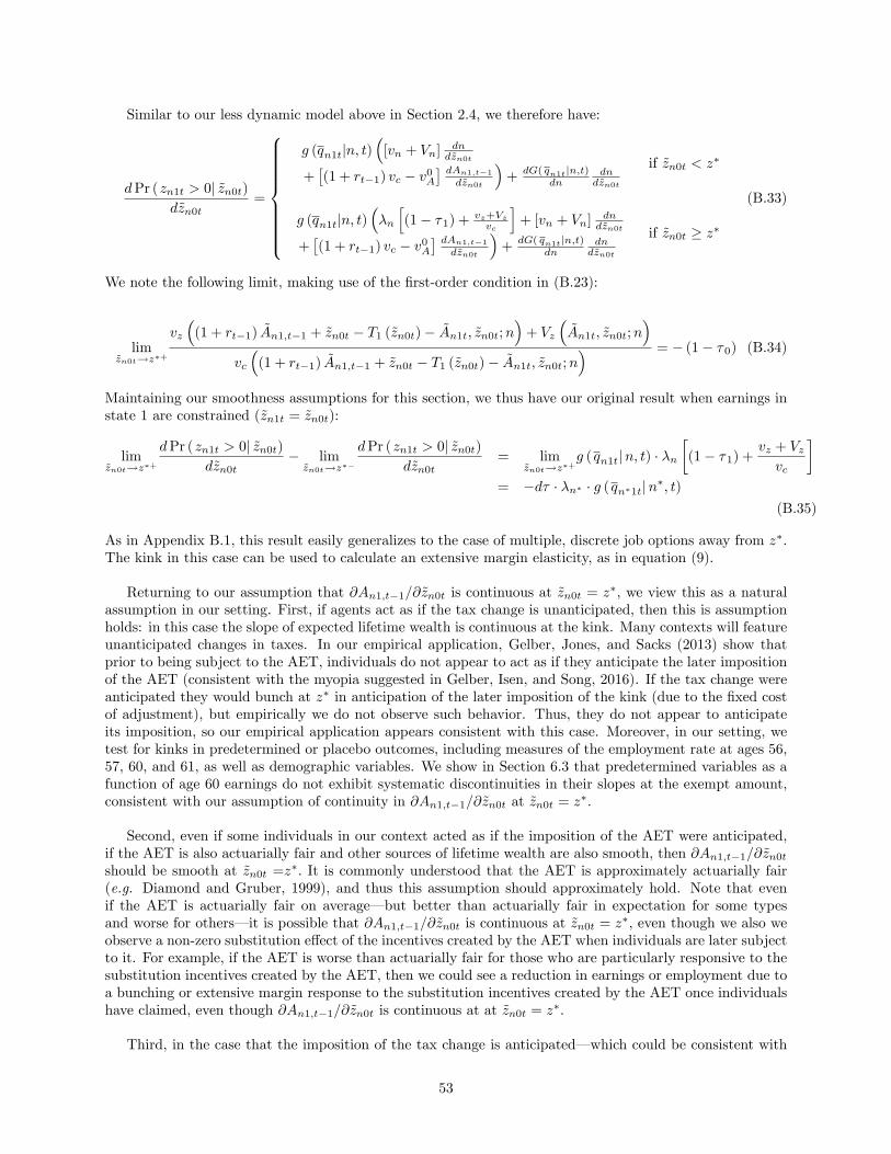
Similar to our less dynamic model above in Section 2.4, we therefore have:

dPr (zn1t > 0| zn0t)

dzn0t=

g (qn1t|n, t)(

[vn + Vn] dndzn0t

+[(1 + rt−1) vc − v0

A

] dAn1,t−1dzn0t

)+ dG( qn1t|n,t)

dndndzn0t

if zn0t < z∗

g (qn1t|n, t)(λn

[(1− τ1) + vz+Vz

vc

]+ [vn + Vn] dn

dzn0t

+[(1 + rt−1) vc − v0

A

] dAn1,t−1dzn0t

)+ dG( qn1t|n,t)

dndndzn0t

if zn0t ≥ z∗

(B.33)

We note the following limit, making use of the first-order condition in (B.23):

limzn0t→z∗+

vz

((1 + rt−1) An1,t−1 + zn0t − T1 (zn0t)− An1t, zn0t;n

)+ Vz

(An1t, zn0t;n

)vc

((1 + rt−1) An1,t−1 + zn0t − T1 (zn0t)− An1t, zn0t;n

) = − (1− τ0) (B.34)

Maintaining our smoothness assumptions for this section, we thus have our original result when earnings instate 1 are constrained (zn1t = zn0t):

limzn0t→z∗+

dPr (zn1t > 0| zn0t)

dzn0t− limzn0t→z∗−

dPr (zn1t > 0| zn0t)

dzn0t= lim

zn0t→z∗+g (qn1t|n, t) · λn

[(1− τ1) +

vz + Vzvc

]= −dτ · λn∗ · g (qn∗1t|n∗, t)

(B.35)

As in Appendix B.1, this result easily generalizes to the case of multiple, discrete job options away from z∗.The kink in this case can be used to calculate an extensive margin elasticity, as in equation (9).

Returning to our assumption that ∂An1,t−1/∂zn0t is continuous at zn0t = z∗, we view this as a naturalassumption in our setting. First, if agents act as if the tax change is unanticipated, then this is assumptionholds: in this case the slope of expected lifetime wealth is continuous at the kink. Many contexts will featureunanticipated changes in taxes. In our empirical application, Gelber, Jones, and Sacks (2013) show thatprior to being subject to the AET, individuals do not appear to act as if they anticipate the later impositionof the AET (consistent with the myopia suggested in Gelber, Isen, and Song, 2016). If the tax change wereanticipated they would bunch at z∗ in anticipation of the later imposition of the kink (due to the fixed costof adjustment), but empirically we do not observe such behavior. Thus, they do not appear to anticipateits imposition, so our empirical application appears consistent with this case. Moreover, in our setting, wetest for kinks in predetermined or placebo outcomes, including measures of the employment rate at ages 56,57, 60, and 61, as well as demographic variables. We show in Section 6.3 that predetermined variables as afunction of age 60 earnings do not exhibit systematic discontinuities in their slopes at the exempt amount,consistent with our assumption of continuity in ∂An1,t−1/∂zn0t at zn0t = z∗.

Second, even if some individuals in our context acted as if the imposition of the AET were anticipated,if the AET is also actuarially fair and other sources of lifetime wealth are also smooth, then ∂An1,t−1/∂zn0t

should be smooth at zn0t =z∗. It is commonly understood that the AET is approximately actuarially fair(e.g. Diamond and Gruber, 1999), and thus this assumption should approximately hold. Note that evenif the AET is actuarially fair on average– but better than actuarially fair in expectation for some typesand worse for others– it is possible that ∂An1,t−1/∂zn0t is continuous at zn0t = z∗, even though we also weobserve a non-zero substitution effect of the incentives created by the AET when individuals are later subjectto it. For example, if the AET is worse than actuarially fair for those who are particularly responsive to thesubstitution incentives created by the AET, then we could see a reduction in earnings or employment due toa bunching or extensive margin response to the substitution incentives created by the AET once individualshave claimed, even though ∂An1,t−1/∂zn0t is continuous at at zn0t = z∗.

Third, in the case that the imposition of the tax change is anticipated– which could be consistent with

53

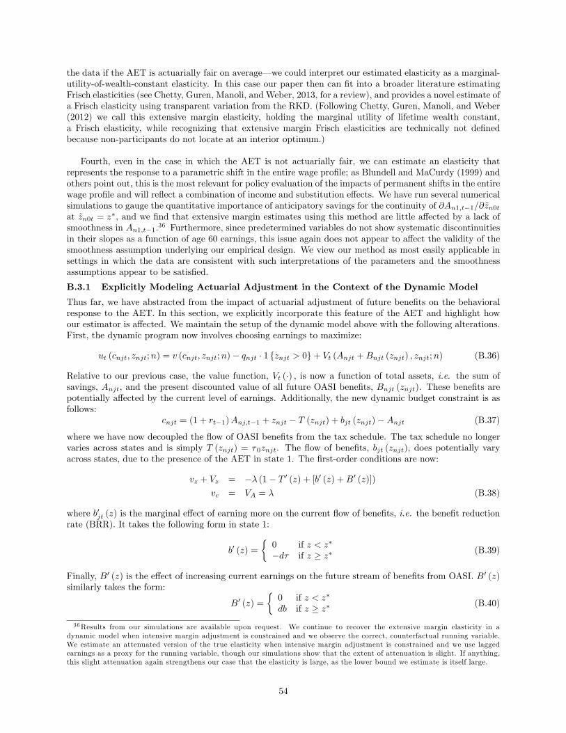
the data if the AET is actuarially fair on average– we could interpret our estimated elasticity as a marginal-utility-of-wealth-constant elasticity. In this case our paper then can fit into a broader literature estimatingFrisch elasticities (see Chetty, Guren, Manoli, and Weber, 2013, for a review), and provides a novel estimate ofa Frisch elasticity using transparent variation from the RKD. (Following Chetty, Guren, Manoli, and Weber(2012) we call this extensive margin elasticity, holding the marginal utility of lifetime wealth constant,a Frisch elasticity, while recognizing that extensive margin Frisch elasticities are technically not definedbecause non-participants do not locate at an interior optimum.)

Fourth, even in the case in which the AET is not actuarially fair, we can estimate an elasticity thatrepresents the response to a parametric shift in the entire wage profile; as Blundell and MaCurdy (1999) andothers point out, this is the most relevant for policy evaluation of the impacts of permanent shifts in the entirewage profile and will reflect a combination of income and substitution effects. We have run several numericalsimulations to gauge the quantitative importance of anticipatory savings for the continuity of ∂An1,t−1/∂zn0t

at zn0t = z∗, and we find that extensive margin estimates using this method are little affected by a lack ofsmoothness in An1,t−1.36 Furthermore, since predetermined variables do not show systematic discontinuitiesin their slopes as a function of age 60 earnings, this issue again does not appear to affect the validity of thesmoothness assumption underlying our empirical design. We view our method as most easily applicable insettings in which the data are consistent with such interpretations of the parameters and the smoothnessassumptions appear to be satisfied.

B.3.1 Explicitly Modeling Actuarial Adjustment in the Context of the Dynamic Model

Thus far, we have abstracted from the impact of actuarial adjustment of future benefits on the behavioralresponse to the AET. In this section, we explicitly incorporate this feature of the AET and highlight howour estimator is affected. We maintain the setup of the dynamic model above with the following alterations.First, the dynamic program now involves choosing earnings to maximize:

ut (cnjt, znjt;n) = v (cnjt, znjt;n)− qnjt · 1 {znjt > 0}+ Vt (Anjt +Bnjt (znjt) , znjt;n) (B.36)

Relative to our previous case, the value function, Vt (·) , is now a function of total assets, i.e. the sum ofsavings, Anjt, and the present discounted value of all future OASI benefits, Bnjt (znjt). These benefits arepotentially affected by the current level of earnings. Additionally, the new dynamic budget constraint is asfollows:

cnjt = (1 + rt−1)Anj,t−1 + znjt − T (znjt) + bjt (znjt)−Anjt (B.37)

where we have now decoupled the flow of OASI benefits from the tax schedule. The tax schedule no longervaries across states and is simply T (znjt) = τ0znjt. The flow of benefits, bjt (znjt), does potentially varyacross states, due to the presence of the AET in state 1. The first-order conditions are now:

vz + Vz = −λ (1− T ′ (z) + [b′ (z) +B′ (z)])

vc = VA = λ (B.38)

where b′jt (z) is the marginal effect of earning more on the current flow of benefits, i.e. the benefit reductionrate (BRR). It takes the following form in state 1:

b′ (z) =

{0 if z < z∗

−dτ if z ≥ z∗ (B.39)

Finally, B′ (z) is the effect of increasing current earnings on the future stream of benefits from OASI. B′ (z)similarly takes the form:

B′ (z) =

{0 if z < z∗

db if z ≥ z∗ (B.40)

36Results from our simulations are available upon request. We continue to recover the extensive margin elasticity in adynamic model when intensive margin adjustment is constrained and we observe the correct, counterfactual running variable.We estimate an attenuated version of the true elasticity when intensive margin adjustment is constrained and we use laggedearnings as a proxy for the running variable, though our simulations show that the extent of attenuation is slight. If anything,this slight attenuation again strengthens our case that the elasticity is large, as the lower bound we estimate is itself large.

54

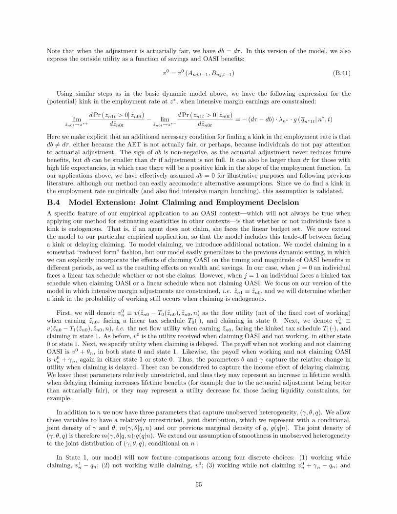
Note that when the adjustment is actuarially fair, we have db = dτ . In this version of the model, we alsoexpress the outside utility as a function of savings and OASI benefits:

v0 = v0 (Anj,t−1, Bnj,t−1) (B.41)

Using similar steps as in the basic dynamic model above, we have the following expression for the(potential) kink in the employment rate at z∗, when intensive margin earnings are constrained:

limzn0t→z∗+

dPr (zn1t > 0| zn0t)

dzn0t− limzn0t→z∗−

dPr (zn1t > 0| zn0t)

dzn0t= − (dτ − db) · λn∗ · g (qn∗1t|n∗, t)

Here we make explicit that an additional necessary condition for finding a kink in the employment rate is thatdb 6= dτ , either because the AET is not actually fair, or perhaps, because individuals do not pay attentionto actuarial adjustment. The sign of db is non-negative, as the actuarial adjustment never reduces futurebenefits, but db can be smaller than dτ if adjustment is not full. It can also be larger than dτ for those withhigh life expectancies, in which case there will be a positive kink in the slope of the employment function. Inour applications above, we have effectively assumed db = 0 for illustrative purposes and following previousliterature, although our method can easily accomodate alternative assumptions. Since we do find a kink inthe employment rate empirically (and also find intensive margin bunching), this assumption is validated.

B.4 Model Extension: Joint Claiming and Employment DecisionA specific feature of our empirical application to an OASI context– which will not always be true whenapplying our method for estimating elasticities in other contexts– is that whether or not individuals face akink is endogenous. That is, if an agent does not claim, she faces the linear budget set. We now extendthe model to our particular empirical application, so that the model includes this trade-off between facinga kink or delaying claiming. To model claiming, we introduce additional notation. We model claiming in asomewhat “reduced form”fashion, but our model easily generalizes to the previous dynamic setting, in whichwe can explicitly incorporate the effects of claiming OASI on the timing and magnitude of OASI benefits indifferent periods, as well as the resulting effects on wealth and savings. In our case, when j = 0 an individualfaces a linear tax schedule whether or not she claims. However, when j = 1 an individual faces a kinked taxschedule when claiming OASI or a linear schedule when not claiming OASI. We focus on our version of themodel in which intensive margin adjustments are constrained, i.e. zn1 ≡ zn0, and we will determine whethera kink in the probability of working still occurs when claiming is endogenous.

First, we will denote v0n ≡ v(zn0 − T0(zn0), zn0, n) as the flow utility (net of the fixed cost of working)

when earning zn0, facing a linear tax schedule T0(·), and claiming in state 0. Next, we denote v1n ≡

v(zn0 − T1(zn0), zn0, n), i.e. the net flow utility when earning zn0, facing the kinked tax schedule T1(·), andclaiming in state 1. As before, v0 is the utility received when claiming OASI and not working, in either state0 or state 1. Next, we specify utility when claiming is delayed. The payoffwhen not working and not claimingOASI is v0 + θn, in both state 0 and state 1. Likewise, the payoff when working and not claiming OASIis v0

n + γn, again in either state 1 or state 0. Thus, the parameters θ and γ capture the relative change inutility when claiming is delayed. These can be considered to capture the income effect of delaying claiming.We leave these parameters relatively unrestricted, and thus they may represent an increase in lifetime wealthwhen delaying claiming increases lifetime benefits (for example due to the actuarial adjustment being betterthan actuarially fair), or they may represent a utility decrease for those facing liquidity constraints, forexample.

In addition to n we now have three parameters that capture unobserved heterogeneity, (γ, θ, q). We allowthese variables to have a relatively unrestricted, joint distribution, which we represent with a conditional,joint density of γ and θ, m(γ, θ|q, n) and our previous marginal density of q, g(q|n). The joint density of(γ, θ, q) is thereforem(γ, θ|q, n)·g(q|n). We extend our assumption of smoothness in unobserved heterogeneityto the joint distribution of (γ, θ, q), conditional on n .

In State 1, our model will now feature comparisons among four discrete choices: (1) working whileclaiming, v1

n − qn; (2) not working while claiming, v0; (3) working while not claiming v0n + γn − qn; and

55

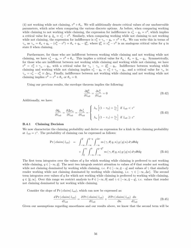
(4) not working while not claiming, v0 + θn. We will additionally denote critical values of our unobservableparameters, which arise when comparing the various discrete options. As before, when comparing workingwhile claiming to not working while claiming, the expression for indifference is v1

n − qn = v0, which impliesa critical value for q, qn ≡ v1

n − v0. Similarly, when comparing working while not claiming to not workingwhile not claiming, the expression for indifference is v0

n + γn − qn = v0 + θn. We can write this in terms ofγn as γn = θn + qn − (v0

n − v0) = θn + qn − q0n, where q

0n ≡ v0

n − v0 is an analogous critical value for q instate 0 when claiming.

Furthermore, for those who are indifferent between working while claiming and not working while notclaiming, we have v1

n − qn = v0 + θn. This implies a critical value for θn : θn = qn − qn. Symmetrically,for those who are indifferent between not working while claiming and working while not claiming, we havev0 = v0

n + γn − qn, with a critical value for γn : γn = q0n − qn. Indifference between working while

claiming and working while not claiming implies v1n − qn = v0

n + γn − qn, and a critical value for γn is:γn = v1

n − v0n ≡ ∆vn. Finally, indifference between not working while claiming and not working while not

claiming implies v0 = v0 + θn or θn = 0.

Using our previous results, the envelope theorem implies the following:

∂q0n

∂zn0=

∂v0n

∂zn0= 0 (B.42)

Additionally, we have:

∂qn∂zn0

=∂∆vn∂zn0

=∂v1

n

∂zn0=

λn

[(1− τ0) + vz

vc

]if zn0 < z∗

λn

[(1− τ1) + vz

vc

]if zn0 ≥ z∗

(B.43)

B.4.1 Claiming Decision

We now characterize the claiming probability and derive an expression for a kink in the claiming probabilityat zn0 = z∗. The probability of claiming can be expressed as follows:

Pr (claim| zn0) =

∫ q

−∞

∫ q−q

−∞

∫ ∆v

−∞m (γ, θ| q, n) g (q|n) dγdθdq

+

∫ ∞q

∫ 0

−∞

∫ q−q0

−∞m (γ, θ| q, n) g (q|n) dγdθdq (B.44)

The first term integrates over the values of q for which working while claiming is preferred to not workingwhile claiming, q ∈ [−∞, q]. The next two integrals restrict attention to values of θ that render not workingwhile not claiming dominated by working while claiming, i.e. θ ∈ [−∞, q − q] and values of γ that similarlyrender working while not claiming dominated by working while claiming, i.e. γ ∈ [−∞,∆v]. The secondterm integrates over values of q for which not working while claiming is preferred to working while claiming,q ∈ [q,∞]. Over this range we restrict analysis to θ ∈ [−∞, 0] and γ ∈ [−∞, q − q], i.e. values that rendernot claiming dominated by not working while claiming.

Consider the slope of Pr (claim| zn0), which can now be expressed as:

dPr (claim| zn0)

dzn0=∂ Pr (claim| zn0)

∂zn0+∂ Pr (claim| zn0)

∂n

dn

dzn0(B.45)

Given our assumptions regarding smoothness and our results above, we know that the second term will be

56

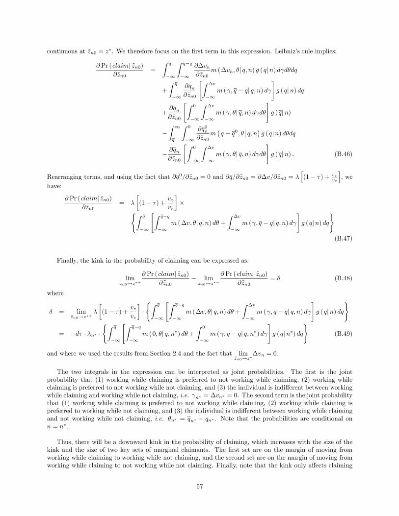
continuous at zn0 = z∗. We therefore focus on the first term in this expression. Leibniz’s rule implies:

∂ Pr (claim| zn0)

∂zn0=

∫ q

−∞

∫ q−q

−∞

∂∆vn∂zn0

m (∆vn, θ| q, n) g (q|n) dγdθdq

+

∫ q

−∞

∂qn∂zn0

[∫ ∆v

−∞m (γ, q − q| q, n) dγ

]g (q|n) dq

+∂qn∂zn0

[∫ 0

−∞

∫ ∆v

−∞m (γ, θ| q, n) dγdθ

]g (q|n)

−∫ ∞q

∫ 0

−∞

∂q0n

∂zn0m(q − q0, θ

∣∣ q, n) g (q|n) dθdq

− ∂qn∂zn0

[∫ 0

−∞

∫ ∆v

−∞m (γ, θ| q, n) dγdθ

]g (q|n) . (B.46)

Rearranging terms, and using the fact that ∂q0/∂zn0 = 0 and ∂q/∂zn0 = ∂∆v/∂zn0 = λ[(1− τ) + vz

vc

], we

have:

∂ Pr (claim| zn0)

∂zn0= λ

[(1− τ) +

vzvc

]×{∫ q

−∞

[∫ q−q

−∞m (∆v, θ| q, n) dθ +

∫ ∆v

−∞m (γ, q − q| q, n) dγ

]g (q|n) dq

}(B.47)

Finally, the kink in the probability of claiming can be expressed as:

limzn0→z∗+

∂ Pr (claim| zn0)

∂zn0− limzn0→z∗−

∂ Pr (claim| zn0)

∂zn0= δ (B.48)

where

δ = limzn0→z∗+

λ

[(1− τ) +

vzvc

]·{∫ q

−∞

[∫ q−q

−∞m (∆v, θ| q, n) dθ +

∫ ∆v

−∞m (γ, q − q| q, n) dγ

]g (q|n) dq

}

= −dτ · λn∗ ·{∫ q

−∞

[∫ q−q

−∞m (0, θ| q, n∗) dθ +

∫ 0

−∞m (γ, q − q| q, n∗) dγ

]g (q|n∗) dq

}(B.49)

and where we used the results from Section 2.4 and the fact that limzn0→z∗

∆vn = 0.

The two integrals in the expression can be interpreted as joint probabilities. The first is the jointprobability that (1) working while claiming is preferred to not working while claiming, (2) working whileclaiming is preferred to not working while not claiming, and (3) the individual is indifferent between workingwhile claiming and working while not claiming, i.e. γn∗ = ∆vn∗ = 0. The second term is the joint probabilitythat (1) working while claiming is preferred to not working while claiming, (2) working while claiming ispreferred to working while not claiming, and (3) the individual is indifferent between working while claimingand not working while not claiming, i.e. θn∗ = qn∗ − qn∗ . Note that the probabilities are conditional onn = n∗.

Thus, there will be a downward kink in the probability of claiming, which increases with the size of thekink and the size of two key sets of marginal claimants. The first set are on the margin of moving fromworking while claiming to working while not claiming, and the second set are on the margin of moving fromworking while claiming to not working while not claiming. Finally, note that the kink only affects claiming

57

among those for whom working while claiming is optimal. Therefore, the only relevant shifting is fromworking while claiming to either state of not claiming.

B.4.2 Extensive Margin Response with Endogenous Claiming

We now consider the extensive margin choice of whether to work, allowing for an endogenous claimingresponse. The probability of having positive earnings in state 1 is now:

Pr (zn1 > 0| zn0) =

∫ q

−∞

[∫ q−q

−∞

∫ ∞−∞

m (γ, θ| q, n) dγdθ +

∫ ∞q−q

∫ ∞θ+q−q0

m (γ, θ| q, n) dγdθ

]g (q|n) dq

+

∫ ∞q

[∫ 0

−∞

∫ ∞q−q0

m (γ, θ| q, n) dγdθ +

∫ ∞0

∫ ∞θ+q−q0

m (γ, θ| q, n) dγdθ

]g (q|n) dq

(B.50)

The probability is comprised of four terms. The first two terms correspond to values of q that render workingwhile claiming preferable to not working while claiming. The first term in this set captures individuals forwhom working while claiming also dominates not working while not claiming. In this case, the individualwill always work, regardless of the value of γ. The second term captures individuals for whom not workingwhile not claiming dominates working while claiming. In this case, only those who prefer working while notclaiming to not working while not claiming will work. The second set of terms likewise covers the two settingsin which not working while claiming dominates working while claiming, but the individual still decides towork. Put another way, an agent will work when max(v1

n − q, v0n + γ − q) > max(v0, v0 + θ).

As in the case of claiming above, we focus on the discontinuity in the partial derivative of this probability,∂ Pr (zn1 > 0|zn0) /∂zn0. Leibniz’s rule again implies:

∂ Pr (zn1 > 0| zn0)

∂zn0=

∫ q

−∞

{∂qn∂zn0

[∫ ∞−∞

m (γ, q − q| q, n) dγ −∫ ∞

∆v

m (γ, q − q| q, n) dγ

]+

∫ ∞q−q

∂q0n

∂zn0m(θ + q − q0, θ

∣∣ q, n) dθ} g (q|n) dq

+∂q

∂zn0

[∫ 0

−∞

∫ ∞−∞

m (γ, θ| q, n) dγdθ +

∫ ∞0

∫ ∞θ+4v

m (γ, θ| q, n) dγdθ

]g ( q|n)

+

∫ ∞q

{∂q0

∂zn0

[∫ 0

−∞m(q − q0, θ

∣∣ q, n) dγdθ +

∫ ∞0

m(θ + q − q0, θ

∣∣ q, n) dγdθ]} g (q|n) dq

− ∂q

∂zn0

[∫ 0

−∞

∫ ∞4v

m (γ, θ| q, n) dγdθ +

∫ ∞0

∫ ∞θ+4v

m (γ, θ| q, n) dγdθ

]g ( q|n) .

(B.51)

Once again relying on the fact that ∂q0/∂zn0 = 0 and ∂q/∂zn0 = ∂∆v/∂zn0 = λ[(1− τ) + vz

vc

], we can

rearrange terms to yield:

∂ Pr (zn1 > 0|zn0)

∂zn0= λ

[(1− τ) +

vzvc

]×{[∫ 0

−∞

∫ 4v−∞

m (γ, θ| q, n) dγdθ

]g ( q|n)

+

∫ q

−∞

∫ 4v−∞

m (γ, q − q| q, n) g (q|n) dγdq

}. (B.52)

The kink in the probability of having positive earnings can now be expressed as:

limzn0→z∗+

dPr (zn1 > 0|zn0)

dzn0− limzn0→z∗−

dPr (zn1 > 0|zn0)

dzn0= β, (B.53)

58

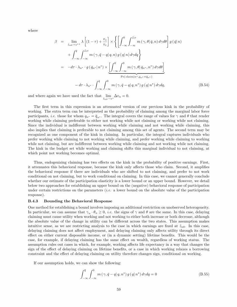
where

β = limzn0→z∗+

λ

[(1− τ) +

vzvc

]×{[∫ 0

−∞

∫ 4v−∞

m (γ, θ| q, n) dγdθ

]g ( q|n)

+

∫ q

−∞

∫ 4v−∞

m (γ, q − q| q, n) g (q|n) dγdq

}

= −dτ · λn∗ · g ( qn∗ |n∗)×[∫ 0

−∞

∫ 0

−∞m (γ, θ| qn∗ , n∗) dγdθ

]︸ ︷︷ ︸

Pr( claim|n∗,qn∗=qn∗ )

− dτ · λn∗ ·∫ q

−∞

∫ 0

−∞m (γ, q − q| q, n∗) g (q|n∗) dγdq, (B.54)

and where again we have used the fact that limzn0→z∗

∆vn = 0.

The first term in this expression is an attenuated version of our previous kink in the probability ofworking. The extra term can be interpreted as the probability of claiming among the marginal labor forceparticipants, i.e. those for whom qn∗ = qn∗ . The integral covers the range of values for γ and θ that renderworking while claiming preferable to either not working while not claiming or working while not claiming.Since the individual is indifferent between working while claiming and not working while claiming, thisalso implies that claiming is preferable to not claiming among this set of agents. The second term may berecognized as one component of the kink in claiming. In particular, the integral captures individuals whoprefer working while claiming to not working while claiming, and prefer working while claiming to workingwhile not claiming, but are indifferent between working while claiming and not working while not claiming.The kink in the budget set while working and claiming shifts this marginal individual to not claiming, atwhich point not working becomes optimal.

Thus, endogenizing claiming has two effects on the kink in the probability of positive earnings. First,it attenuates this behavioral response, because the kink only affects those who claim. Second, it amplifiesthe behavioral response if there are individuals who are shifted to not claiming, and prefer to not workconditional on not claiming, but to work conditional on claiming. In this case, we cannot generally concludewhether our estimate of the participation elasticity is a lower bound or an upper bound. However, we detailbelow two approaches for establishing an upper bound on the (negative) behavioral response of participationunder certain restrictions on the parameters (i.e. a lower bound on the absolute value of the participationresponse).

B.4.3 Bounding the Behavioral Response

One method for establishing a bound involves imposing an additional restriction on unobserved heterogeneity.In particular, we can assume that γn · θn ≥ 0, i.e. the signs of γ and θ are the same. In this case, delayingclaiming must cause utility when working and not working to either both increase or both decrease, althoughthe absolute value of the change in utility can be different across the two states. This assumption makesintuitive sense, as we are restricting analysis to the case in which earnings are fixed at zn0. In this case,delaying claiming does not affect employment, and delaying claiming only affects utility through its directeffect on either current disposable income, or (in a dynamic setting) lifetime benefits. This would be thecase, for example, if delaying claiming has the same effect on wealth, regardless of working status. Theassumption rules out cases in which, for example, working affects life expectancy in a way that changes thesign of the effect of delaying claiming on lifetime benefits, or a case in which working relaxes a borrowingconstraint and the effect of delaying claiming on utility therefore changes sign, conditional on working.

If our assumption holds, we can show the following:∫ q

−∞

∫ 0

−∞m (γ, q − q| q, n∗) g (q|n∗) dγdq = 0 (B.55)

59

The reason why this probability becomes zero is as follows. First, we are restricting attention to values ofq ≤ q. In addition, we are fixing the value of θ = q − q ≥ 0. However, we are also restricting analysis toindividuals for whom γ ≤ 0. Given our assumption that the signs of γ and θ must be the same, this set mustbe of measure zero.

In this case, we can simplify our two kinks above as follows:

δ = −dτ · λn∗ ×∫ q

−∞

∫ q−q

−∞m (0, θ| q, n∗) g (q|n∗) dθdq (B.56)

β = −dτ · λn∗ × g ( q|n∗)[∫ 0

−∞

∫ 0

−∞m (γ, θ| qn∗ , n∗) dγdθ

]︸ ︷︷ ︸

Pr( claim|n∗,qn∗=qn∗ )

(B.57)

The kink in participation we estimate is now a weak upper bound on a negative kink (i.e. the absolute valueof the kink in participation we estimate is a lower bound on the kink that would obtain absent a claimingresponse). This implies that our observed elasticity will be a lower bound. Note that the probability ofclaiming that attenuates the behavioral response is local to marginal labor force participants, i.e. q = q, andthus is not the same as the population probability of claiming at zn0 = z∗.

If we are not willing to impose the above restrictions on the joint distribution of γ and θ, we can stillachieve a lower bound. Using the results from the previous two sections, we have:

β − δ = −dτ · λn∗ × g ( qn∗ |n∗, t)[∫ 0

−∞

∫ 0

−∞m (γ, θ| qn∗ , n∗) dγdθ

]+dτ · λn∗ ×

∫ q

−∞

∫ q−q

−∞m (0, θ| q, n∗) g (q|n∗) dθdq (B.58)

Again, this difference in kinks provides an upper bound on the negative kink in participation. Note thatthis bound is not guaranteed to be negative. However, in cases in which the kink in claiming is relativelynegligible– as appears to be the case in our empirical application– it is possible to establish a non-trivialupper bound on the kink and, by extension, a lower bound on the employment elasticity. Furthermore, ifthere is no detectable kink in claiming, then simply rescaling the kink in employment by the share claimingis suffi cient to adjust for endogenous claiming.

C Procedure for estimating excess massAs we explain in Gelber, Jones, and Sacks (2013), we seek to estimate the “excess mass”at the kink, i.e. thefraction of the sample that locates at the kink under the kinked tax schedule but not under the linear taxschedule. Following a standard procedure in the literature (e.g. Saez, 2010; Chetty, Friedman, Olsen, andPistaferri, 2011), we estimate the counterfactual density (i.e. the density in the presence of a linear budgetset) by fitting a smooth polynomial to the earnings density away from the kink, and then estimating the“excess”mass in the region of the kink that occurs above this smooth polynomial.

Specifically, for each earnings bin zi, we calculate pi, the proportion of the sample with earnings in therange [zi − k/2, zi + k/2). The earnings bins are normalized by distance-to-kink, so that for zi = 0, pi is thefraction of all individuals with earnings in the range [0, k). To estimate bunching, we assume that pi can bewritten as:

pi =

D∑d=0

βd · (zi)d +

k∑j=−k

γ · 1{zi = j}+ εi (C.59)

and run this regression (where 1 denotes the indicator function and j denotes the bin). This equationexpresses the earnings distribution as a degree D polynomial, plus a set of indicators for each bin within kδof the kink, where δ is the bin width. In our empirical application, we choose D = 7, δ = 500 and k = 6as our baseline (so that six bins are excluded from the polynomial estimation). We control for a baseline

60

seventh-degree polynomial through the density following Chetty, Friedman, Olsen, and Pistaferri (2011).The parameter γ reflects the excess density near the kink.

Our measure of excess mass is M = 2kγ, the estimated excess probability of locating at the kink (relativeto the polynomial term). This measure depends on the counterfactual density near the kink, so to obtain ameasure of excess mass that is comparable at the kink, we scale by the predicted density that we would obtainif there were a linear budget set. This is just the constant term in the polynomial, since zi is the distanceto zero. Thus, our estimate of normalized excess mass is B = M

β0. We calculate standard errors using the

delta method. We calculate the density in each bin by dividing the number of beneficiaries in the bin by thetotal number of beneficiaries within the bandwidth; note that this normalization should not affect the excessnormalized mass or the estimated density, because dividing by the total number of beneficiaries within the

bandwidth affects the numerator (i.e. M) and denominator (i.e. β0) of the expression for B(

= Mβ0

)in equal

proportions and therefore should have no impact on B.

61

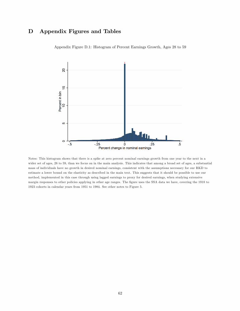
D Appendix Figures and Tables

Appendix Figure D.1: Histogram of Percent Earnings Growth, Ages 28 to 59

Notes: This histogram shows that there is a spike at zero percent nominal earnings growth from one year to the next in a

wider set of ages, 28 to 59, than we focus on in the main analysis. This indicates that among a broad set of ages, a substantial

mass of individuals have no growth in desired nominal earnings, consistent with the assumptions necessary for our RKD to

estimate a lower bound on the elasticity as described in the main text. This suggests that it should be possible to use our

method, implemented in this case through using lagged earnings to proxy for desired earnings, when studying extensive

margin responses to other policies applying in other age ranges. The figure uses the SSA data we have, covering the 1918 to

1923 cohorts in calendar years from 1951 to 1984. See other notes to Figure 5.

62

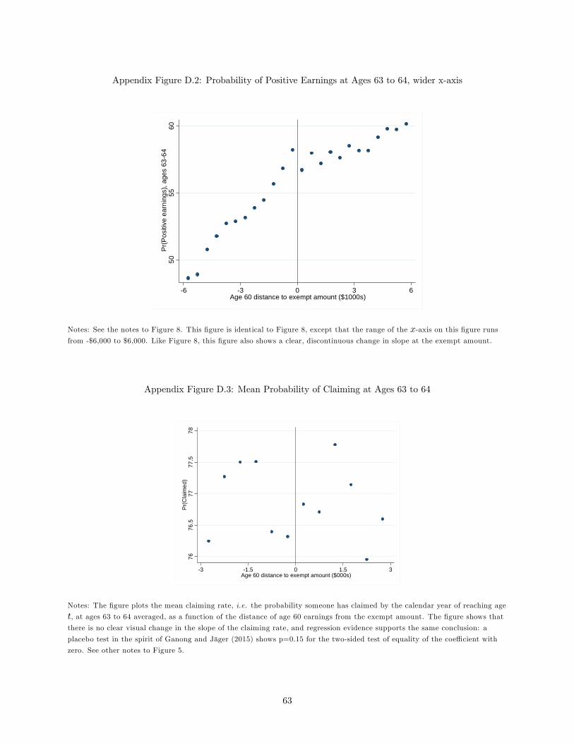
Appendix Figure D.2: Probability of Positive Earnings at Ages 63 to 64, wider x-axis

5055

60P

r(P

ositi

ve e

arni

ngs)

, age

s 63

­64

­6 ­3 0 3 6Age 60 distance to exempt amount ($1000s)

Notes: See the notes to Figure 8. This figure is identical to Figure 8, except that the range of the x-axis on this figure runsfrom -$6,000 to $6,000. Like Figure 8, this figure also shows a clear, discontinuous change in slope at the exempt amount.

Appendix Figure D.3: Mean Probability of Claiming at Ages 63 to 64

7676

.577

77.5

78P

r(Cla

imed

)

­3 ­1.5 0 1.5 3Age 60 distance to exempt amount ($000s)

Notes: The figure plots the mean claiming rate, i.e. the probability someone has claimed by the calendar year of reaching age

t, at ages 63 to 64 averaged, as a function of the distance of age 60 earnings from the exempt amount. The figure shows that

there is no clear visual change in the slope of the claiming rate, and regression evidence supports the same conclusion: a

placebo test in the spirit of Ganong and Jäger (2015) shows p=0.15 for the two-sided test of equality of the coeffi cient with

zero. See other notes to Figure 5.

63

Appendix Table D.1: Robustness of Elasticity Estimates(1) (2)

Baseline WithSpecification Controls

Linear 0.49 0.45(0.19)*** (0.18)***

N 95,960 104,665Quadratic 0.66 0.60

(0.27)*** (0.24)***N 160,785 172,979Cubic 0.82 0.68

(0.28)*** (0.28)***N 273,421 326,782

Notes: The table presents robustness checks on the main elasticity estimates in Table 5. The “with controls” column shows

the kink in the employment probability when we control for dummies for year of birth, sex, and race. Robust standard errors,

using the procedure of Calonico, Cattaneo, and Titiunik (2014), are reported in parentheses. The number of individuals

included in each “reduced form” regression (13) is shown below the standard error. See other notes to Table 2.

Appendix Table D.2: RKD Elasticity Estimates using Regression-Based First Stage(1) (2) (3) (4) (5) (6) (7)Full Non- High Prior Low PriorSample Men Women White White Earnings Earnings

First Stage Kink -4.00 -3.25 -3.99 -3.88 -3.09 -3.76 -3.82(0.01)*** (0.01)*** (0.01)*** (0.01)*** (0.01)*** (0.01)*** (0.01)***

Elasticity 0.59 0.37 0.60 0.59 0.64 0.62 0.52(0.23)*** (0.29) (0.26)*** (0.22)*** (0.68) (0.35)* (0.11)***

N 95,960 68,971 66,251 93,722 39,271 19,574 101,709

Notes: See notes to Table 5. Relative to Table 5, the elasticities differ here because we use a linear RKD to estimate the first

stage kink in the ANTR (reported in the first row), rather than using the analytic expression as in Table 5.

Appendix Table D.3: Elasticity Estimates Accounting for Claiming(1) (2) (3) (4) (5) (6) (7)Full Non- High Prior Low PriorSample Men Women White White Earnings Earnings

Elasticity 0.63 0.32 0.65 0.61 0.53 0.62 0.53(0.25)*** (0.25) (0.28)** (0.23)*** (0.56) (0.35)* (0.12)***

N 95,960 68,971 66,251 93,722 39,271 19,574 101,709

Notes: See notes to Table 5. As explained in the main text, we calculate these elasticities by inflating the Table 5 elasticities

by 29.9 percent, to account for claiming behavior. Among those with age 60 earnings below the kink, but not more than

$2,797 below the kink, 74.5 percent of the sample claims by age 63, and 79.5 by age 64. We calculate 29.9 percent as

100·(1/[(0.795+0.745)/2]-1).

64