Using genetic algorithms to Þnd technical trading rules1finance.wharton.upenn.edu/~allenf/download/Vita/genetic.pdf · Genetic algo- rithms have also been applied to theoretical

*Corresponding author. Tel.: 215 898 3628; fax: 215 573 2207; e-mail: [email protected].

1Helpful comments were made by Adam Dunsby, Lawrence Fisher, Steven Kimbrough, PaulKleindorfer, Michele Kreisler, James Laing, Josef Lakonishok, George Mailath, and seminarparticipants at Institutional Investor, J.P. Morgan, the NBER Asset Pricing Program, Ohio StateUniversity, Purdue University, the Santa Fe Institute, Rutgers University, Stanford University,University of California, Berkeley, University of Michigan, University of Pennsylvania, Universityof Utah, Washington University (St. Louis), and the 1995 AFA Meetings in Washington, D.C. Weare particularly grateful to Kenneth R. French (the referee), and G. William Schwert (the editor) fortheir suggestions. Financial support from the National Science Foundation is gratefully acknow-ledged by the first author and from the Academy of Finland by the second and from theGeewax-Terker Program in Financial Instruments by both. Correspondence should be addressed toFranklin Allen, The Wharton School, University of Pennsylvania, Philadelphia, PA 19104-6367.

Journal of Financial Economics 51 (1999) 245—271

Using genetic algorithms to find technical trading rules1

Franklin Allen!,*, Risto Karjalainen"

! The Wharton School, University of Pennsylvania, Philadelphia, PA 19104, USA" Merrill Lynch & Co., Inc., Mercury Asset Management, 33 King William Street, London, EC4R 9AS, UK

Received 12 October 1995; received in revised form 7 April 1998

Abstract

We use a genetic algorithm to learn technical trading rules for the S&P 500 index usingdaily prices from 1928 to 1995. After transaction costs, the rules do not earn consistentexcess returns over a simple buy-and-hold strategy in the out-of-sample test periods. Therules are able to identify periods to be in the index when daily returns are positive andvolatility is low and out when the reverse is true. These latter results can largely beexplained by low-order serial correlation in stock index returns. ( 1999 ElsevierScience S.A. All rights reserved.

JEL classification: C61; G11; G14

Keywords: Trading rules; Genetic algorithms; Excess returns

1. Introduction

Genetic algorithms belong to a class of machine learning algorithms that havebeen successfully used in a number of research areas. There is a growing interest

0304-405X/99/$— see front matter ( 1999 Elsevier Science S.A. All rights reservedPII: S 0 3 0 4 - 4 0 5 X ( 9 8 ) 0 0 0 5 2 - X

in their use in financial economics but so far there has been little formal analysis.The purpose of this paper is to demonstrate how they can be used to findtechnical trading rules. The techniques can be easily extended to include othertypes of information such as fundamental and macro-economic data as well aspast prices.

Over the years there has been a large literature on the effectiveness ofvarious technical trading rules. The majority of this literature has found thatsuch rules do not make money. For instance, Alexander (1961) tests a numberof ‘filter rules’, which advise a trader to buy if the price rises by a fixed percentage(5%, say) and sell if the price declines by the same percentage. Althoughsuch rules appear to yield returns above the buy-and-hold strategy for theDow Jones and Standard & Poor’s stock indices, Alexander (1964)concludes that adjusted for transaction costs, the filter rules are notprofitable. These conclusions are supported by the results of Fama andBlume (1966), who find no evidence of profitable filter rules for the 30Dow Jones stocks. On the whole, the studies during the 1960s provide littleevidence of profitable trading rules, and lead Fama (1970) to dismiss technicalanalysis as a futile undertaking. In a more recent study, Brock et al. (1992)consider the performance of various simple moving average rules in the absenceof transaction costs. They find that these rules identify periods to be in themarket (long the Dow Jones index) when returns are high and volatility is lowand vice versa.

All of this previous literature uses ad hoc specifications of trading rules. Thisleads to a problem of data snooping whereby the ex post specification of rulescan lead to biased test results. We show how genetic algorithms can be used toderive trading rules that are not ad hoc but are in a sense optimal. Thisapproach avoids a potential bias caused by ex post selection, because the rulesare chosen by a machine learning algorithm using price data available before thestart of the test period.

We consider trading rules for the Standard & Poor’s composite index(S&P 500). Our results confirm those of previous studies. They suggestthat the markets for these stocks are efficient in the sense that it is notpossible to make money after transaction costs using technical trading rules.Like Brock et al. (1992), we are able to identify periods to be in the marketwhen returns are high and volatility is low and out when the reverse istrue. A study of how the rules work indicates that many have tradingpatterns that are like those generated by simple moving average rules.This suggests they are exploiting well-known low-order serial correlation inmarket indices (see, e.g., Fisher, 1966; French and Roll, 1986; Lo and MacKin-lay, 1990).

Section 2 describes genetic algorithms. Section 3 shows how the rules arefound and evaluated, and addresses the robustness of the results. Section 4contains concluding remarks.

246 F. Allen, R. Karjalainen/Journal of Financial Economics 51 (1999) 245—271

2There are many variations of the basic genetic algorithm. The version described here employscontinuous reproduction, as opposed to a more conventional approach where the whole generationis replaced by a new one. The idea of continuous reproduction was originally proposed by Holland(1975), and developed by Syswerda (1989) and Whitley (1989). Similarly to Whitley, we also userank-based selection, instead of the more common method of computing the selection probabilitieson the basis of scaled fitness values

2. Genetic algorithms

2.1. Introduction to evolutionary algorithms

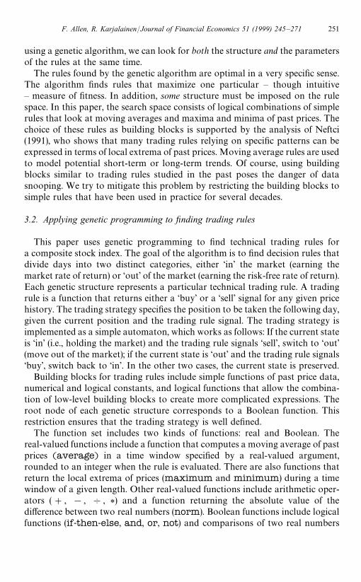
Genetic algorithms constitute a class of search, adaptation, and optimizationtechniques based on the principles of natural evolution. Genetic algorithms weredeveloped by Holland (1962, 1975). Other evolutionary algorithms includeevolution strategies (Rechenberg, 1973; Schwefel, 1981), evolutionary program-ming (Fogel et al., 1966), classifier systems (Holland, 1976, 1980), and geneticprogramming Koza (1992). For an introduction to genetic algorithms, seeBeasley et al. (1993).

An evolutionary algorithm maintains a population of solution candidates andevaluates the quality of each solution candidate according to a problem-specificfitness function, which defines the environment for the evolution. New solutioncandidates are created by selecting relatively fit members of the population andrecombining them through various operators. Specific evolutionary algorithmsdiffer in the representation of solutions, the selection mechanism, and the detailsof the recombination operators.

In a genetic algorithm, solution candidates are represented as characterstrings from a given (often binary) alphabet. In a particular problem, a mappingbetween these genetic structures and the original solution space has to bedeveloped, and a fitness function has to be defined. The fitness functionmeasures the quality of the solution corresponding to a genetic structure. In anoptimization problem, the fitness function simply computes the value of theobjective function. In other problems, fitness could be determined by a co-evolutionary environment consisting of other genetic structures. For instance,one could study the equilibrium properties of game-theoretic problems wherebya population of strategies evolves with the fitness of each strategy defined as theaverage payoff against the other members of the population.

A genetic algorithm starts with a population of randomly generated solutioncandidates.2 The next generation is created by recombining promising candi-dates. The recombination involves two parents chosen at random from thepopulation, with the selection probabilities biased in favor of the relatively fitcandidates. The parents are recombined through a ‘crossover’ operator, whichsplits the two genetic structures apart at randomly chosen locations, and joins

F. Allen, R. Karjalainen/Journal of Financial Economics 51 (1999) 245—271 247

a piece from each parent to create an ‘offspring’ (as a safeguard against the lossof genetic diversity, random ‘mutations’ are occasionally introduced into theoffspring). The algorithm evaluates the fitness of the offspring and replaces oneof the relatively unfit members of the population. New genetic structures areproduced until the generation is completed. Successive generations are createdin the same manner until a well-defined termination criterion is satisfied. Thefinal population provides a collection of solution candidates, one or more ofwhich can be applied to the original problem.

The theoretical foundation of genetic algorithms is laid out in Holland (1975).Maintaining a population of solution candidates makes the search processparallel, allowing an efficient exploration of the solution space. In addition tothis explicit parallelism, genetic algorithms are implicitly parallel in that theevaluation of the fitness of a specific genetic structure yields information aboutthe quality of a very large number of ‘schemata’, or building blocks. Theso-called schema theorem shows that a genetic algorithm automatically allocatesan exponentially increasing number of trials to the best observed schemata. Thisleads to a favorable tradeoff between exploitation of promising directions of thesearch space and exploration of less-frequented regions of the space (see alsoVose, 1991). However, there is no general result guaranteeing the convergence ofa genetic algorithm to the global optimum.

Evolutionary algorithms offer a number of advantages over more traditionaloptimization methods. They can be applied to problems with a nondifferentiableor discontinuous objective function, to which gradient-based methods such asGauss—Newton would not be applicable. They are also useful when the objectivefunction has several local optima. Because of the stochastic nature of theselection and recombination operators, evolutionary algorithms are less likelyto converge to local maxima than hill-climbing or gradient-type methods.Evolutionary optimization methods can often be successfully applied when thesize of the search space poses difficulties for other optimizations methods. Insuch problems, the parallel trial-and-error process is an efficient way to reducethe uncertainty about the search space.

Evolutionary algorithms do have limitations. Maintaining a population ofgenetic structures leads to an increase in execution time, due to the number oftimes the objective function must be evaluated. Since evolutionary algorithmsembody very little problem-specific knowledge, they are unlikely to performbetter and can be less efficient than special-purpose algorithms in well-under-stood domains. Despite the schema theorem, the lack of a theoretical conver-gence result is a weakness. In differentiable problems, an evolutionary algorithmmay indeed converge to a point where the gradient is nonzero. This can happenif there is not enough genetic variation left in the population by the time thealgorithm approaches the optimum. However, this last drawback can often beavoided by switching to hill-climbing when the genetic algorithm makes nofurther progress.


One should not view genetic algorithms or other members of the family asa replacement for other optimization methods. It is more productive to regardthem as a complement, the usefulness of which depends on the nature of theproblem. Even though evolutionary algorithms are not guaranteed to find theglobal optimum, they can find an acceptable solution relatively quickly in a widerange of problems.

Evolutionary algorithms have been applied to a large number of problems inengineering, computer science, cognitive science, economics, managementscience, and other fields (for references, see Goldberg, 1989; Booker et al., 1989).The number of practical applications has been rising steadily, especially sincethe late 1980s. Typical business applications involve production planning,job-shop scheduling, and other difficult combinatorial problems. Genetic algo-rithms have also been applied to theoretical questions in economic markets, totime series forecasting, and to econometric estimation (see, e.g., Marimon et al.,1990; Dorsey and Mayer, 1995). String-based genetic algorithms have beenapplied to finding market-timing strategies based on fundamental data for stockand bond markets by Bauer (1994).

2.2. Genetic programming

In traditional genetic algorithms, genetic structures are represented as charac-ter strings of fixed length. This representation is adequate for many problems,but it is restrictive when the size or the form of the solution cannot be assessedbeforehand. Genetic programming, developed by Koza (1992), is an extension ofgenetic algorithms that partly alleviates the restrictions of the fixed-lengthrepresentation of genetic structures. For the purposes of this paper, the mainadvantage of genetic programming is the ability to represent different tradingrules in a natural way.

In genetic programming, solution candidates are represented as hierarchicalcompositions of functions. In these tree-like structures, the successors of eachnode provide the arguments for the function identified with the node. Theterminal nodes (i.e., nodes with no successors) correspond to the input data. Theentire tree is also interpreted as a function, which is evaluated recursively bysimply evaluating the root node of the tree. The structure of the solutioncandidates is not specified a priori. Instead, a set of functions is defined asbuilding blocks to be recombined by the genetic algorithm.

The function set is chosen in a way appropriate to the particular problemunder study. Koza focuses much of his work on genetic structures that includeonly functions of a single type. However, genetic programming possesses noinherent limitations about the types of functions, as long as a so-called ‘closure’property is satisfied. This property holds if all possible combinations of subtreesresult in syntactically valid composite functions. Closure is needed to ensurethat the recombination operator is well defined.


Genetic programming also maintains a population of genetic structures. Theinitial population consists of random trees. The root node of a tree is chosen atrandom among functions of the same type as the desired composite function.Each argument of that function is then selected among the functions of theappropriate type, proceeding recursively down the tree until a function with noarguments (a terminal node) is reached. The evolution takes place much as in thebasic genetic algorithms, selecting relatively fit solution candidates to be recom-bined and replacing unfit individuals with the offspring.

In genetic programming, the crossover operator recombines two solutioncandidates by replacing a randomly selected subtree in the first parent witha subtree from the second parent. If different types of functions are used withina tree, the appropriate procedure involves choosing the crossover node atrandom within the first parent, and then choosing the crossover node within thesecond parent among the nodes of the same type as the crossover node in thefirst tree. Mutations are introduced by using a randomly generated tree in placeof the second parent with a small probability.

Koza applies genetic programming to a diverse array of problems, rangingfrom symbolic integration to the evolution of ant colonies to the optimal controlof a broom balanced on top of a moving cart. As one specific example illustra-ting the effectiveness of the algorithm, Koza (1992, Chapter 8) applies geneticprogramming to learning the correct truth table for the so-called six-multiplexerproblem. In this problem, there are six binary inputs and one binary output. Thecorrect logical mapping must specify the correct output for each of the 26 inputcombinations. Hence, the size of the search space is 264+1019. Using geneticprogramming, no more than 160,000 individual solution candidates are neces-sary to find the correct solution with a 99% probability. By comparison, the bestsolution found in a random search over ten million truth tables produced thecorrect output for only 52 out of 64 possible input combinations.

3. Finding and evaluating trading rules

3.1. Ex ante optimal trading rules

Most of the previous trading rule studies have sought to test whether particu-lar kinds of technical rules have forecasting ability. A machine learning ap-proach to finding testable trading rules sheds light on a question that is subtlydifferent. Instead of asking whether specific rules work, we seek to find outwhether in a certain sense optimal rules can be used to forecast future returns.Allowing a genetic algorithm to compose the trading rules avoids much of thearbitrariness involved in choosing which rules to test. Were we to use a moretraditional search method, we would have to decide the form of the trading rulesbefore searching through the parameter space for the chosen class of rules. By


using a genetic algorithm, we can look for both the structure and the parametersof the rules at the same time.

The rules found by the genetic algorithm are optimal in a very specific sense.The algorithm finds rules that maximize one particular — though intuitive— measure of fitness. In addition, some structure must be imposed on the rulespace. In this paper, the search space consists of logical combinations of simplerules that look at moving averages and maxima and minima of past prices. Thechoice of these rules as building blocks is supported by the analysis of Neftci(1991), who shows that many trading rules relying on specific patterns can beexpressed in terms of local extrema of past prices. Moving average rules are usedto model potential short-term or long-term trends. Of course, using buildingblocks similar to trading rules studied in the past poses the danger of datasnooping. We try to mitigate this problem by restricting the building blocks tosimple rules that have been used in practice for several decades.

3.2. Applying genetic programming to finding trading rules

This paper uses genetic programming to find technical trading rules fora composite stock index. The goal of the algorithm is to find decision rules thatdivide days into two distinct categories, either ‘in’ the market (earning themarket rate of return) or ‘out’ of the market (earning the risk-free rate of return).Each genetic structure represents a particular technical trading rule. A tradingrule is a function that returns either a ‘buy’ or a ‘sell’ signal for any given pricehistory. The trading strategy specifies the position to be taken the following day,given the current position and the trading rule signal. The trading strategy isimplemented as a simple automaton, which works as follows: If the current stateis ‘in’ (i.e., holding the market) and the trading rule signals ‘sell’, switch to ‘out’(move out of the market); if the current state is ‘out’ and the trading rule signals‘buy’, switch back to ‘in’. In the other two cases, the current state is preserved.

Building blocks for trading rules include simple functions of past price data,numerical and logical constants, and logical functions that allow the combina-tion of low-level building blocks to create more complicated expressions. Theroot node of each genetic structure corresponds to a Boolean function. Thisrestriction ensures that the trading strategy is well defined.

The function set includes two kinds of functions: real and Boolean. Thereal-valued functions include a function that computes a moving average of pastprices (average) in a time window specified by a real-valued argument,rounded to an integer when the rule is evaluated. There are also functions thatreturn the local extrema of prices (maximum and minimum) during a timewindow of a given length. Other real-valued functions include arithmetic oper-ators (#, !, %, *) and a function returning the absolute value of thedifference between two real numbers (norm). Boolean functions include logicalfunctions (if-then-else, and, or, not) and comparisons of two real numbers


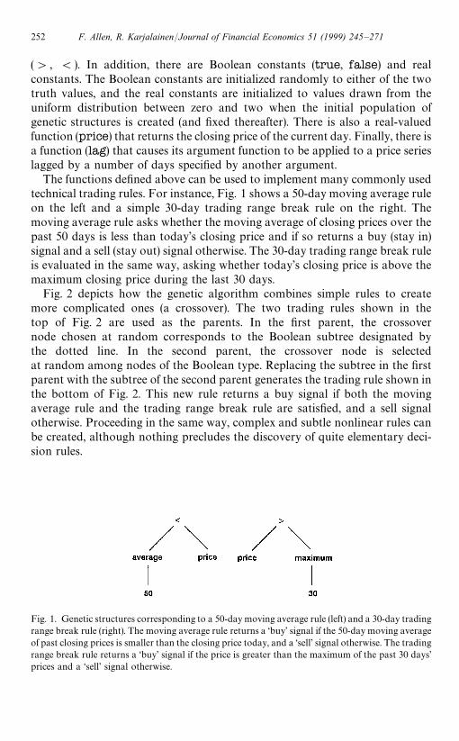
Fig. 1. Genetic structures corresponding to a 50-day moving average rule (left) and a 30-day tradingrange break rule (right). The moving average rule returns a ‘buy’ signal if the 50-day moving averageof past closing prices is smaller than the closing price today, and a ‘sell’ signal otherwise. The tradingrange break rule returns a ‘buy’ signal if the price is greater than the maximum of the past 30 days’prices and a ‘sell’ signal otherwise.

(', (). In addition, there are Boolean constants (true, false) and realconstants. The Boolean constants are initialized randomly to either of the twotruth values, and the real constants are initialized to values drawn from theuniform distribution between zero and two when the initial population ofgenetic structures is created (and fixed thereafter). There is also a real-valuedfunction (price) that returns the closing price of the current day. Finally, there isa function (lag) that causes its argument function to be applied to a price serieslagged by a number of days specified by another argument.

The functions defined above can be used to implement many commonly usedtechnical trading rules. For instance, Fig. 1 shows a 50-day moving average ruleon the left and a simple 30-day trading range break rule on the right. Themoving average rule asks whether the moving average of closing prices over thepast 50 days is less than today’s closing price and if so returns a buy (stay in)signal and a sell (stay out) signal otherwise. The 30-day trading range break ruleis evaluated in the same way, asking whether today’s closing price is above themaximum closing price during the last 30 days.

Fig. 2 depicts how the genetic algorithm combines simple rules to createmore complicated ones (a crossover). The two trading rules shown in thetop of Fig. 2 are used as the parents. In the first parent, the crossovernode chosen at random corresponds to the Boolean subtree designated bythe dotted line. In the second parent, the crossover node is selectedat random among nodes of the Boolean type. Replacing the subtree in the firstparent with the subtree of the second parent generates the trading rule shown inthe bottom of Fig. 2. This new rule returns a buy signal if both the movingaverage rule and the trading range break rule are satisfied, and a sell signalotherwise. Proceeding in the same way, complex and subtle nonlinear rules canbe created, although nothing precludes the discovery of quite elementary deci-sion rules.


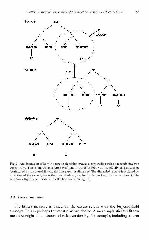
Fig. 2. An illustration of how the genetic algorithm creates a new trading rule by recombining twoparent rules. This is known as a ‘crossover’, and it works as follows. A randomly chosen subtree(designated by the dotted line) in the first parent is discarded. The discarded subtree is replaced bya subtree of the same type (in this case Boolean), randomly chosen from the second parent. Theresulting offspring rule is shown in the bottom of the figure.

3.3. Fitness measure

The fitness measure is based on the excess return over the buy-and-holdstrategy. This is perhaps the most obvious choice. A more sophisticated fitnessmeasure might take account of risk aversion by, for example, including a term


that penalizes for large daily losses or for large drawdowns of wealth, accordingto the risk attitude of a particular investor.

The fitness of a rule is computed as the excess return over the buy-and-holdstrategy during a training period. To evaluate the fitness of a trading rule, it isapplied to each trading day to divide the days into periods in (earning themarket return) or out of the market (earning a risk-free return). The continuous-ly compounded return is then computed, and the buy-and-hold return and thetransaction costs are subtracted to determine the fitness of the rule. The simplereturn from a single trade (buy at date b

i, sell at s

i) is thus

ni"

Psi

Pbi

]1!c

1#c!1"expC

si+

t/bi`1

rtD]

1!c

1#c!1

"expCsi+

t/bi`1

rt#log

1!c

1#cD!1, (1)

where Ptis the closing price (or level of the composite stock index) on day t,

rt"log P

t!log P

t~1is the daily continuously compounded return, and c

denotes the one-way transaction cost (expressed as a fraction of the price). Let¹ be the number of trading days and let r

&(t) denote the risk-free rate on day t.

Define two indicator variables, I"(t) and I

4(t), equal to one if a rule signals buy

and sell, respectively, and zero otherwise with the indicator variables satisfyingthe relation I

"(t)]I

4(t)"0 ∀t. Lastly, let n denote the number of trades, i.e., the

number of buy signals followed by a subsequent sell signal (an open position inthe last day is forcibly closed). Then, the continuously compounded return fora trading rule can be computed as

r"T+t/1

rtI"(t)#

T+t/1

r&(t)I

4(t)#nlog

1!c

1#c, (2)

and the total (simple) return is n"er!1. The return for the buy-and-holdstrategy (buy the first day, sell the last day) is

r")"

T+t/1

rt#log

1!c

1#c, (3)

and the excess return or fitness for a trading rule is given by

Dr"r!r")

. (4)

As short sales can only be made on an uptick, the implementation ofsimultaneous short sales for a composite stock index is difficult. Consequently,we do not consider short positions. Results by Sweeney (1988) suggest that largeinstitutional investors can achieve one-way transaction costs in the range of


3The computer code for finding trading rules for the S&P 500 index can be obtained usinganonymous ftp from opim.wharton.upenn.edu (log in as ‘anonymous’ and type your e-mailaddress as password). The C code is located in the directory /pub/programs/risto/jfe99.

0.1—0.2% (at least after the mid-1970s), and floor traders can achieve consider-ably lower costs. However, realistic transaction costs including the marketimpact are likely to be higher for most investors. Initially, we use one-waytransaction costs of 0.25%. We also investigate the robustness of the results withtransaction costs of 0.1% or 0.5%.

One issue that needs to be addressed in the design of the genetic algorithm isthe possibility of overfitting the training data. The task of inferring technicaltrading rules relies on the assumption that there are some underlying regulari-ties in the data. However, there are going to be patterns arising from noise, andthe trick is to find trading rules that generalize beyond the training sample. Theproblem is common to all methods of non-linear statistical inference, and severalapproaches have been proposed to avoid overfitting. These include reservinga part of the data as a validation set on which to test the predictions, increasingthe amount of training data, penalizing for model complexity, and minimizingthe amount of information needed to describe both the model and the data (fora discussion of overfitting, see Gershenfeld and Weigend, 1993). We reservea selection period immediately following the training period for validation of theinferred trading rules. After each generation, we apply the fittest rule (based onthe excess return in the training period) to the selection period. If the excessreturn in the selection period improves upon the best previously saved rule, thenew rule is saved.

Table 1 summarizes the algorithm used to find trading rules.3 To start with,an initial population of rules is created at random. The algorithm determines thefitness of each trading rule by applying it to the daily data for the S&P 500 indexin the training period. It then creates a new generation of rules by recombiningparts of relatively fit rules in the population. After each generation, the best rulein the population is applied to a selection period. If the rule leads to a higherexcess return than the best rule so far, the new rule is saved. The evolutionterminates when there is no improvement in the selection period for a predeter-mined number of generations, or when a maximum number of generations isreached. The best rule is then applied to the out-of-sample test period immedi-ately following the selection period. If no rule better than the buy-and-holdstrategy in the training period emerges in the maximum number of generations,the trial is abandoned.

We use a population size of 500. The size of the genetic structures is limited to100 nodes and to a maximum of ten levels of nodes. Evolution continues fora maximum of 50 generations, or until there is no improvement for 25 genera-tions. Each trial starts from a different random population.


Table 1One trial of the genetic algorithm used to find technical trading rules

Step 1Create a random rule.Compute the fitness of the rule as the excess return in the training period above the buy-and-holdstrategy.Do this 500 times (this is the intial population).

Step 2Apply the fittest rule in the population to the selection period and compute the excess return.Save this rule as the initial best rule.

Step 3Pick two parent rules at random, using a probability distribution skewed towards the best rule.Create a new rule by breaking the parents apart randomly and recombining the pieces (this isa crossover).Compute the fitness of the rule as the excess return in the training period above the buy-and-holdstrategy.Replace one of the old rules by the new rule, using a probability distribution skewed towards theworst rule.Do this 500 times (this is called one generation).

Step 4Apply the fittest rule in the population to the selection period and compute the excess return.If the excess return improves upon the previous best rule, save as the new best rule.Stop if there is no improvement for 25 generations or after a total of 50 generations. Otherwise, goback to Step 3.

4The authors are grateful to G. William Schwert for providing us with pre-1963 data

3.4. Data

We use daily data for the S&P 500 index from 3 January 1928 to 29 December1995.4 For 1929—1991, the one-month risk-free rates corresponding to Treasurybills are from the Center for Research in Security Prices with Datastreamproviding data for 1992 to 1995. Since the S&P 500 series is clearly nonstation-ary (rising from 17 in early 1928 to 615 by the end of 1995), we transform thedata by dividing each day’s price by a 250-day moving average. The normalizedprices have an order of magnitude around one. Since we use the first year of datafor normalization, the usable data set covers 1929—1995. All test results arebased on the unnormalized data.


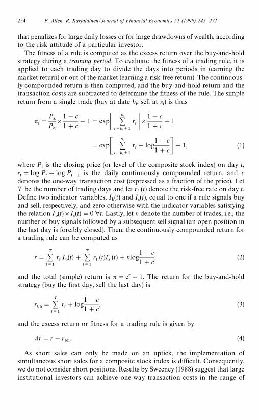
Fig. 3. The yearly excess return over a buy-and-hold strategy and the average number of trades peryear for trading rules found by the genetic algorithm, using 0.25% one-way transaction costs. Eachpoint is labeled with an indicator of the training period, with labels 1, 2,2 corresponding to thetraining periods 1929—1933, 1934—1938, etc.

3.5. Results

To find trading rules for the S&P 500 index, we conduct 100 independenttrials, saving one rule from each trial. We use a one-way transaction cost of0.25% initially. To guard against potential data snooping in the choice of timeperiods, we use ten successive training periods and report the summarizedresults for each case. The five-year training and two-year selection periods startin 1929, 1934, 2, 1974, with the out-of-sample test periods starting in 1936,1941, 2, 1981. For instance, the first trial uses years 1929—1933 as the trainingperiod, 1934—1935 as the selection period, and 1936—1995 as the test period. Foreach of the ten training periods, we carry out ten trials.

We find a total of 89 trading rules in the 100 trials (recall that no rules aresaved from a trial if the excess returns are not positive in the selection period). Asan overview of the results, Fig. 3 shows the average annual excess return and theaverage number of trades per year. The excess returns are predominantlynegative. The trading frequency is relatively low, with an average of 3.8 tradesper year. On average, the rules are long in the market for 57% of the days. Theresults are generally consistent for rules found from different training periods,except for those found in 1929—1935 and 1969—1975. The trading rules fromthese two periods stay mostly out of the market during the test period, which isperhaps not surprising given that both training periods involve substantialnegative returns to stocks.

Panel A of Table 2 summarizes the statistical tests of the out-of-samplereturns with the most reasonable level of transaction costs of 0.25%. The


Tab

le2

Asu

mm

ary

ofth

ete

stre

sultsfo

rtr

adin

gru

lesfo

und

by

the

genet

ical

gorith

mfo

rva

riousle

vels

ofo

ne-w

aytr

ansa

ctio

nco

sts.

Pan

elA

consider

sth

em

ost

reas

onab

leca

seof

0.25

%.P

anel

sB

and

Cco

nsid

er0.

1%an

d0.

5%to

show

these

nsitivi

tyof

there

sults.

Thefir

stco

lum

nsh

ow

sth

ein

-sam

ple

trai

ning

and

sele

ctio

nper

iod,w

ith

aco

rres

pon

ding

out

-of-sa

mpl

ete

stper

iod

star

ting

the

follow

ing

year

and

exte

ndin

gto

the

end

of19

95.K

isth

enu

mber

oft

radin

gru

les

found

by

the

algo

rith

m.E

xces

sde

note

sth

eav

erag

eye

arly

exce

ssre

turn

inth

eout

-of-sa

mple

per

iod

abov

eth

ebuy-

and-

hol

dst

rate

gyaf

ter

tran

sact

ion

cost

s.K

`is

the

num

ber

ofr

ule

sw

ith

apo

sitive

exce

ssre

turn

.Eac

htr

adin

gru

lediv

ides

the

days

into

per

iods‘in

’(lo

ngin

the

mar

ket)

and

‘out

’oft

hem

arket

(ear

ning

arisk

-fre

era

teofr

etur

n).A

vera

geda

ily

retu

rnsduring

‘in’a

nd‘o

ut’p

erio

dsar

ede

not

edby

r "an

dr 4,r

espec

tive

ly,w

ith

thest

andar

dde

viat

ion

ofd

aily

retu

rnsde

not

edby

p "an

dp 4

and

thenum

ber

ofd

aysby

N"an

dN

4.¹*

isth

enum

ber

oft

-sta

tist

icsfo

rr "!

r 4sign

ifica

ntat

the

5%le

vel

In-s

ample

KExc

ess

K`

N"

r "p "

N4

r 4p 4

r "!r 4

¹*

Pan

elA

:¹

rans

action

cost

sof

0.25

%

1929

—35

10!

0.03

360

1614

!0.

0000

680.

0018

7014

202

#0.

0002

200.

0082

19!

0.00

0288

019

34—4

010

!0.

0105

093

74#

0.00

0347

0.00

7652

4940

#0.

0002

630.

0102

97#

0.00

0085

819

39—4

510

!0.

0281

147

46#

0.00

0371

0.01

0881

8081

#0.

0005

820.

0082

64!

0.00

0211

219

44—5

010

!0.

0022

391

12#

0.00

0378

0.00

7665

2305

!0.

0000

290.

0097

77#

0.00

0406

619

49—5

54

!0.

0031

288

72#

0.00

0295

0.00

8337

1236

!0.

0000

510.

0085

47#

0.00

0346

119

54—6

08

#0.

0014

784

12#

0.00

0298

0.00

8506

436

!0.

0008

570.

0080

88#

0.00

1155

319

59—6

510

!0.

0107

068

90#

0.00

0427

0.00

8592

700

!0.

0014

730.

0120

18#

0.00

1900

919

64—7

07

!0.

0386

247

14#

0.00

0519

0.00

8514

1643

!0.

0004

430.

0109

32#

0.00

0962

519

69—7

510

!0.

0440

041

2#

0.00

3290

0.00

8771

4684

#0.

0003

640.

0091

80#

0.00

2926

219

74—8

010

!0.

0359

211

45#

0.00

0183

0.00

3560

2687

#0.

0003

200.

0103

34!

0.00

0137

0

Ave

rage

8.9

!0.

0205

1.7

5529

#0.

0006

040.

0074

3540

91!

0.00

0110

0.00

9566

#0.

0007

143.

6

Pan

elB:¹

rans

action

cost

sof

0.1%

1929

—35

10!

0.03

720

13!

0.00

0181

0.00

2156

1580

4#

0.00

0244

0.00

9116

!0.

0004

240

1934

—40

10!

0.00

315

9254

#0.

0003

710.

0075

7650

60#

0.00

0013

0.00

9707

#0.

0003

5910

1939

—45

10!

0.02

730

3690

#0.

0004

000.

0106

6191

37#

0.00

0225

0.00

7880

#0.

0001

763

1944

—50

10#

0.01

107

9118

#0.

0004

740.

0075

5522

99!

0.00

0580

0.01

0395

#0.

0010

549

1949

—55

10#

0.01

096

8251

#0.

0004

640.

0080

5918

57!

0.00

0430

0.00

9173

#0.

0008

946

1954

—60

8#

0.00

428

8695

#0.

0002

900.

0086

2315

3!

0.00

1043

0.00

8108

#0.

0013

327


1959

—65

10#

0.03

5810

6094

#0.

0006

450.

0081

5114

96!

0.00

1380

0.01

1491

#0.

0020

2510

1964

—70

10!

0.00

135

3439

#0.

0008

160.

0083

0329

18!

0.00

0287

0.01

0288

#0.

0011

0310

1969

—75

10!

0.05

110

2704

#0.

0009

430.

0083

5523

91!

0.00

0275

0.01

0066

#0.

0012

1810

1974

—80

10!

0.04

430

2303

#0.

0008

410.

0085

0015

29!

0.00

0296

0.01

1128

#0.

0011

3710

Ave

rage

9.8

!0.

0102

4.1

5356

#0.

0005

060.

0077

9442

64!

0.00

0381

0.00

9735

#0.

0008

877.

5

Pan

elC

:¹

rans

action

cost

sof

0.5 %

1929

—35

10!

0.02

940

3230

#0.

0000

760.

0023

6312

587

#0.

0001

930.

0073

20!

0.00

0117

019

34—4

010

!0.

0220

078

48#

0.00

0258

0.00

7552

6466

#0.

0001

220.

0094

56#

0.00

0136

819

39—4

510

!0.

0316

052

76#

0.00

0399

0.01

0940

7550

#0.

0007

380.

0079

93!

0.00

0338

019

44—5

05

!0.

0161

088

86#

0.00

0392

0.00

7464

2531

#0.

0000

310.

0113

22#

0.00

0360

319

49—5

52

#0.

0035

194

89#

0.00

0294

0.00

8085

619

!0.

0002

820.

0124

93#

0.00

0576

119

54—6

06

!0.

0001

487

38#

0.00

0285

0.00

8624

110

!0.

0011

680.

0078

57#

0.00

1453

419

59—6

510

!0.

0154

268

81#

0.00

0254

0.00

8425

709

#0.

0001

550.

0125

07#

0.00

0099

119

64—7

00

1969

—75

10!

0.05

120

193

#0.

0025

830.

0107

1949

02#

0.00

0375

0.00

9165

#0.

0022

081

1974

—80

10!

0.05

020

301

#0.

0000

370.

0009

5035

31#

0.00

0404

0.00

9697

!0.

0003

670

Ave

rage

7.3

!0.

0236

0.7

5649

#0.

0005

090.

0072

3643

34#

0.00

0063

0.00

9757

#0.

0004

461.

8


average excess returns after transaction costs are negative for nine out of the tentest periods. In most of the periods, there are only a few rules with positive excessreturns. Hence, the results are consistent with market efficiency. It is interestingto note, however, that in seven out of the ten test periods, the average dailyreturn during ‘in’ periods is higher than the unconditional return, while thereturn during ‘out’ periods is lower. The difference between ‘in’ and ‘out’ returnsis statistically significant for 36 rules out of the total of 89 (the t-statistic for thedifference is

t"(r"!r

4)NAsS

1

N"

#

1

N4B,

where s2 is the sample variance). Also, the standard deviation during ‘in’ days issmaller than during ‘out’ days for most training periods. The volatility of theannual trading rule returns is 10.0%, averaged over the trading rules and overthe different out-of-sample periods. The sample standard deviation of theannual returns for the S&P 500 index during the same period is 14.7%. It is alsointeresting that constructing a ‘portfolio’ of trading rules appears to diversifyrisk in much the same way as adding companies to a stock portfolio. Fora composite trading strategy in which an equal amount of capital is allocated toeach of the rules from a particular trading period, the volatility drops to 8.7%,averaged over the out-of-sample periods.

We investigate the impact of trading costs on the results by carrying out twomore sets of 100 trials, using transaction costs of 0.1% and 0.5% but holding theother parameters fixed. Panel B of Table 2 summarizes the results for lowtransaction costs (0.1%) and Panel C for high transaction costs (0.5%). With lowtransaction costs, the trading frequency is high, with an average of 18 trades peryear. Average excess returns are negative for six out of the ten test periods, againconsistent with market efficiency. The difference between daily returns during‘in’ and ‘out’ periods is positive for nine periods out of ten, and statisticallysignificant for almost all the rules. With high transaction costs, the tradingfrequency drops to an average of 1.4 trades per year. The excess returns arenegative for nine periods out of ten. The difference between daily returns during‘in’ and ‘out’ periods is positive for six periods out of ten, but statisticallysignificant in only a few cases. The pattern of reduced volatility during days longin the market remains similar for different levels of transaction costs. Theproportion of days long in the market is around 56—57% regardless of the levelof transaction costs. These results indicate that while trading rules found usingunrealistically low transaction costs lead to higher returns and better forecastingability, the excess returns above the buy-and-hold strategy generally remainnegative. High transaction costs lead to diminished forecasting ability.

Overall, the out-of-sample results show that the rules found by the geneticalgorithm do not earn consistent excess returns after transaction costs. It is


interesting that in most of the training periods, the rules appear to have someforecasting ability in the sense that the average daily return during daysin the market is higher compared to days out of the market, and the volatilityis generally lower during the days the rules are long in the market. Eventhough the rules do not lead to higher absolute returns than a buy-and-holdstrategy, the reduced volatility might still make them attractive to someinvestors on a risk-adjusted basis. Finally, there appears to be a diversificationbenefit in using a number of trading rules in a portfolio, with the position to betaken in each period determined as a weighted average of the trading rulesignals.

The finding that the trading rules tend to be long in low-volatility periods issomewhat surprising, given that the fitness of the rules does not depend on thevolatility of the returns. However, it is possible to make the case that theobserved pattern is what one might expect based on economic theory. In mostequilibrium models, expected excess returns are positively related to risk asmeasured by the expected volatility (Merton, 1980). French et al. (1987) find thatex post stock market returns are negatively related to the unexpected change involatility, supporting the theoretical risk-return relation. For instance, when thevolatility turns out to be higher than expected, investors revise their volatilityforecasts upwards, requiring higher expected returns in the future, or lowerstock prices and hence lower realized returns at the present. Conversely, whenthe volatility is lower than expected, investors revise their volatility forecastsdownwards, requiring lower expected returns and higher stock prices andrealized returns now. Applied to the present study, high ex post volatility whenthe rules are out of the market would be consistent with the theory if thehigh-volatility periods represent unexpected increases in risk. The trading rulepositions will change when the rules pick up subsequent higher realized returns.Similarly, if the low volatility when the rules are long in the market wereunexpected, the trading rule signals would change when the downwards-revisedexpected returns start to be realized.

3.6. Characterizing the trading rules

There are a number of interesting questions regarding the nature of the rulesfound by the genetic algorithm. This section describes what the rules look likeand analyzes what kind of price behavior triggers the trading rule signals. Weanalyze one rule for each level of transaction costs and for each training period.

The structure and complexity of the rules found by the algorithm vary acrossdifferent trials. The size of the rules varies from nine to 94 nodes, with a depthbetween five and ten levels. While many of the rules appear to be quitecomplicated at first sight, there is often a lot of redundant material in the form ofduplicated subtrees. If some of these subtrees are never visited when the rules areevaluated, seemingly complex tree structures can be effectively similar to much


simpler ones. Consequently, measuring the complexity of the trading rulescannot in general be done by inspection of the tree structures.

One measure of the complexity of the trading rules can be obtained bycomparing the behavior of the rules to a class of simple technical tradingrules. The simple rules are of the form illustrated in Fig. 1. These rules compareone indicator to another and take a position in (out of) the market if thevalue of the first indicator is greater than (less than or equal to) the value of thesecond one. Each indicator is chosen from the set Mmax, min, averageN,and the length of the time window for an indicator is chosen from the set M1, 2, 3,4, 5, 10, 15, 20, 40, 60, 80, 100, 150, 200, 250N. In addition, we considerrules that compare the normalized price to a constant in the range from 0.9 to1.1 with increments of 0.01. For each rule, we retain the combinationof indicators that leads to the highest correlation between the daily positions,after evaluating all the combinations during the appropriate out-of-sampleperiod.

With 0.25% transaction costs, most of the rules can be matched quite wellwith a rule that compares the normalized price to a constant. These rules areeffectively similar to a 250-day moving average rule for unnormalized prices. Intwo periods, there is no close match among the simple rules. With 0.1%transaction costs, about half the rules are similar to a rule that compares thenormalized price to a constant, while the remaining rules resemble either10-to-40-day moving average rules or a trading range break rule comparingtoday’s price to a three-day minimum. With 0.5% transaction costs, rules fromthe early training periods are similar to a rule comparing the normalized price toa constant, while the rules from the late training periods match none of thesimple rules considered.

As an example of what the trading rules look like, let us first consider the bestrule from the training period 1964—1968, learned using transaction costs of0.25%. The tree structure shown in Fig. 4 can be reduced to the expressionprice]minimum(price)!0.0688]price'0.8943. This is roughlyequivalent to a rule that takes a position in the market when normalized pricesare above 0.89 and is out of the market otherwise. If we were to use unno-rmalized prices, an equivalent rule would take a long position when the pricerises within 2% of the 250-day moving average or higher.

Fig. 5a illustrates the price behavior during the trades signaled by this rule.Each line represents the cumulative market return (without transaction costs)for a trade in a long position. When the rule returns a ‘buy’ signal this becomesday 0 and the line represents the price pattern that is realized until the rulereturns a ‘sell’ signal, at which point the line ends. The lines for each trade aresuperimposed on top of each other. Fig. 5a shows that once the rule takes a longposition, it can last up to several years. Fig. 5b shows the cumulative marketreturns after rule 1 switches out of the market. Again each line representsa particular trade. When the rule generates a sell signal this becomes day 0 and


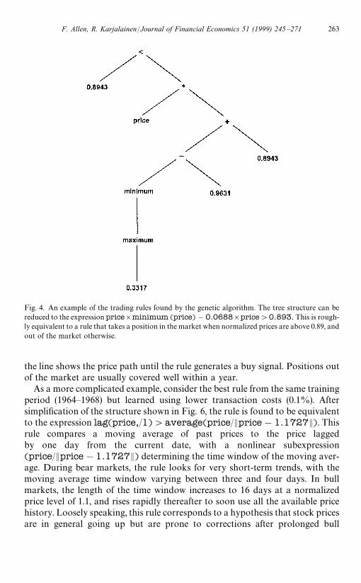
Fig. 4. An example of the trading rules found by the genetic algorithm. The tree structure can bereduced to the expression price]minimum (price)!0.0688]price'0.893. This is rough-ly equivalent to a rule that takes a position in the market when normalized prices are above 0.89, andout of the market otherwise.

the line shows the price path until the rule generates a buy signal. Positions outof the market are usually covered well within a year.

As a more complicated example, consider the best rule from the same trainingperiod (1964—1968) but learned using lower transaction costs (0.1%). Aftersimplification of the structure shown in Fig. 6, the rule is found to be equivalentto the expression lag(price,/1)'average(price/Eprice!1.1727E). Thisrule compares a moving average of past prices to the price laggedby one day from the current date, with a nonlinear subexpression(price/Eprice!1.1727E) determining the time window of the moving aver-age. During bear markets, the rule looks for very short-term trends, with themoving average time window varying between three and four days. In bullmarkets, the length of the time window increases to 16 days at a normalizedprice level of 1.1, and rises rapidly thereafter to soon use all the available pricehistory. Loosely speaking, this rule corresponds to a hypothesis that stock pricesare in general going up but are prone to corrections after prolonged bull


Fig. 5. a. The cumulative market return during each trade going long in the market for a rule foundin 1964—1970 using 0.25% transaction costs. Each line starts when the rule returns a ‘buy’ signal andends when the rule returns a ‘sell’ signal. The graphs for all the trades in the test period of 1971—1995are superimposed on top of each other. b. The cumulative market return during each trade out of themarket for a rule found in 1964—70 using 0.25% transaction costs. Each line starts when the rulereturns a ‘sell’ signal and ends when the rule returns a ‘buy’ signal. The graphs for all the trades in thetest period of 1971—1995 are superimposed on top of each other.

markets. This rule is quick to take a long position in bear markets, but isincreasingly hesitant to do so when prices are high.

Fig. 7a and b show the price behavior during the trades signaled by this rule.The trading frequency is much higher than for the medium-transaction-cost rulefrom the same period. Fig. 7a shows that trades in a long position typically last


Fig. 6. An example of the trading rules found by the genetic algorithm. The tree structure isequivalent to the expression lag(price,1)'average(price/Eprice!1.1727E). This rule com-pares a moving average of past prices to the price lagged by one day from the current date, witha nonlinear subexpression (price/Eprice!1.1727E) determining the time window of the movingaverage.

for one to four weeks. Without transaction costs, most of the trades areprofitable. The rule switches out of the market after a large negative return,consistent with its trend-following nature. Fig. 7b shows that after a sell signalsmall negative returns tend to persist for a couple of weeks. The rule switchesback into the index after a large positive return.

3.7. Robustness of the results

The out-of-sample test results indicate that the trading rules do not earnconsistent excess returns after transaction costs. Nevertheless, they appear tohave some ability to forecast daily returns. In this section, we consider potentialexplanations for this. It is well known that there is low-order serial correlation inmarket indexes (see, e.g., Fisher, 1966; French and Roll, 1986; Lo and MacKin-lay, 1990). We start by considering the effect of incorporating a lag of one day inthe implementation of trades. We then discuss the biases introduced by theexclusion of dividends in our data set. We also address the effect of the 1987stock market crash on the results.


Fig. 7. a. The cumulative market return during each trade going long in the market for a rule foundin 1964—1970 using 0.1% transaction costs. Each line starts when the rule returns a ‘buy’ signal andends when the rule returns a ‘sell’ signal. The graphs for all the trades in the test period of 1971—1995are superimposed on top of each other. b. The cumulative market return during each trade out of themarket for a rule found in 1964—1970 using 0.1% transaction costs. Each line starts when the rulereturns a ‘sell’ signal and ends when the rule returns a ‘buy’ signal. The graphs for all the trades in thetest period of 1971—1995 are superimposed on top of each other.

To test whether the genetic algorithm exploits low-order serial correlation inreturns, the ex post best rules are retested with a one-day lag before the tradingsignals are implemented. Panel A of Table 3 shows the test results without a lagfor 0.25% transaction costs. Panel B of Table 3 shows the results with a one-day


Tab

le3

Tes

tre

sults

forth

eex

post

bes

ttr

adin

gru

les

found

by

the

genet

ical

gorith

m,u

sing

one-

way

tran

sact

ion

cost

sof0.

25%

.Pan

elA

show

sth

ere

sults

with

trad

ing

sign

alsco

mpu

ted

and

imple

men

ted

usin

gth

esa

me

day

’scl

osing

price

.Pan

elB

show

sth

ere

sultsw

ith

trad

ing

sign

alsdel

ayed

byone

day.

Inea

chpa

nel,

the

firs

tco

lum

nsh

owsth

ein

-sam

ple

trai

ning

and

sele

ctio

nper

iod,w

ith

aco

rres

pondin

gout

-of-sa

mpl

ete

stpe

riod

star

ting

the

follo

win

gye

aran

dex

tend

ing

toth

een

dof

1995

.Exce

ssden

otes

the

aver

age

year

lyex

cess

retu

rnin

the

out

-of-sa

mpl

eper

iod

abov

eth

ebuy

-and-

hol

dst

rate

gyaf

ter

tran

sact

ion

cost

s.E

ach

trad

ing

rule

div

ides

the

days

into

per

iods

‘in’(lo

ngin

the

mar

ket

)an

d‘o

ut’

ofth

em

arke

t(e

arnin

ga

risk

-fre

era

teof

retu

rn).

Ave

rage

dai

lyre

turn

sdu

ring

‘in’a

nd‘o

ut’

per

iodsar

eden

ote

dby

r "an

dr 4,r

espec

tive

ly,w

ith

the

stan

dar

dde

viat

ion

ofda

ilyre

turn

sden

oted

by

p "an

dp 4

and

the

num

ber

ofday

sby

N"

and

N4.¹

-sta

tist

ics

are

give

nin

pare

nth

eses

In-s

ample

Exc

ess

N"

r "(t)

pN

4r 4

(t)

pr "!

r 4(t)

Pan

elA

:¹es

tre

sults

usin

gsign

als

com

pute

dan

dim

plem

ente

dus

ing

the

clos

ing

pric

e

1934

—40

!0.

0030

9952

#0.

0003

88(#

0.96

6)0.

0073

9043

62#

0.00

0047

(!1.

663)

0.00

9888

#0.

0003

40(2

.277

)19

39—4

5!

0.01

8862

44#

0.00

0430

(#1.

180)

0.00

8606

6583

#0.

0001

34(!

1.13

9)0.

0080

61#

0.00

0296

(2.0

09)

1944

—50

#0.

0048

9085

#0.

0004

10(#

0.96

6)0.

0078

0523

32!

0.00

0136

(!2.

328)

0.00

9660

#0.

0005

47(2

.864

)19

49—5

5#

0.01

0785

66#

0.00

0411

(#1.

243)

0.00

8012

1542

!0.

0005

95(!

3.71

0)0.

0103

10#

0.00

1007

(4.3

26)

1954

—60

#0.

0023

6236

#0.

0003

93(#

0.88

9)0.

0076

5426

12!

0.00

0036

(!1.

576)

0.01

0563

#0.

0004

29(2

.137

)19

59—6

5!

0.01

7865

58#

0.00

0531

(#1.

865)

0.00

8597

1032

!0.

0015

39(!

6.02

3)0.

0107

63#

0.00

2070

(6.9

06)

1964

—70

#0.

0008

4913

#0.

0003

87(#

1.86

5)0.

0077

5114

44!

0.00

0002

(!1.

113)

0.01

3195

#0.

0003

89(1

.402

)19

74—8

0#

0.00

5229

06#

0.00

0527

(#0.

558)

0.00

7903

926

!0.

0000

21(!

1.17

6)0.

0137

45#

0.00

0548

(1.5

05)

Ave

rage

!0.

0020

6808

#0.

0004

350.

0079

6526

04!

0.00

0269

0.01

0773

#0.

0007

03

Pan

elB

:¹

est

resu

lts

usin

gsign

als

dela

yed

byon

eda

y

1934

—40

!0.

0069

9951

#0.

0003

66(#

0.76

4)0.

0074

3343

63#

0.00

0097

(!1.

314)

0.00

9816

#0.

0002

69(1

.801

)19

39—4

5!

0.01

7762

43#

0.00

0439

(#1.

250)

0.00

8673

6584

#0.

0001

26(!

1.20

6)0.

0079

92#

0.00

0313

(2.1

27)

1944

—50

#0.

0010

9084

#0.

0003

91(#

0.80

4)0.

0077

7823

33!

0.00

0064

(!1.

938)

0.00

9749

#0.

0004

55(2

.385

)19

49—5

5#

0.01

5885

65#

0.00

0288

(#0.

242)

0.00

7964

1543

#0.

0000

92(!

0.72

2)0.

0105

53#

0.00

0196

(0.8

42)

1954

—60

#0.

0040

6235

#0.

0004

03(#

0.95

7)0.

0077

2026

13!

0.00

0059

(!1.

697)

0.01

0445

#0.

0004

62(2

.300

)19

59—6

5!

0.08

0765

57#

0.00

0243

(!0.

043)

0.00

8574

1033

#0.

0002

91(#

0.13

8)0.

0110

46!

0.00

0047

(!0.

158)

1964

—70

!0.

0121

4912

#0.

0003

22(#

0.13

1)0.

0084

2014

45#

0.00

0221

(!0.

289)

0.01

1721

#0.

0001

01(0

.364

)19

74—8

0!

0.01

7229

05#

0.00

0412

(#0.

072)

0.00

9004

927

#0.

0003

41(!

0.15

1)0.

0114

31#

0.00

0070

(0.1

93)

Ave

rage

!0.

0184

6808

#0.

0003

580.

0081

9626

04#

0.00

0131

0.01

0344

#0.

0002

27


lag. Using delayed signals, the average difference in returns during ‘in’ and ‘out’days drops from seven to two basis points. The pattern of reduced volatilityduring days long in the market is not affected by the delay. In the case of 0.1%transaction costs, a one-day delay removes all the difference between returnsduring ‘in’ and ‘out’ days. In the case of 0.5% transaction costs, there is littledifference between the returns with or without a one-day lag. These results,together with simple characterizations of the rule obtained in the previoussection, indicate that with low or medium transaction costs, most of theforecasting ability can be explained by low-order positive serial correlation instock index returns. It is interesting that the trading rules produced by thegenetic algorithm apparently exploit a well-known feature of the data.

The computation of the S&P 500 index ignores the payment of dividends onthe component stocks. Ignoring dividends affects the results in two ways. Anyseasonality can distort the results, if trading rules happen to pick periods to beout of the market when a disproportionate number of stocks go ex-dividend.There is, in fact, a rather pronounced yearly pattern in dividend payments,which tend to be concentrated in February, May, August, and November(Luskin, 1987, pp. 140,141). The clustering of dividends is unlikely to affect theresults, because the calendar dates are not part of the information set of thegenetic algorithm. However, ignoring the dividend yield leads to underestima-tion of the buy-and-hold return. The trading rule returns are underestimated,too, but to a lesser extent. Comparing the results for a subperiod using a value-weighted index of NYSE and AMEX stocks with and without dividends showsthat the main effect of the dividends is to lower the annual returns as expected,while the pattern in daily returns and volatility is not affected (the details areavailable upon request).

Since the trading rules use daily data, the extreme market volatility aroundthe stock market crash in October 1987 crash could have a potentially largeimpact on the results. We explore these effects by testing the rules on a data setthat excludes the crash. Since the level of the S&P 500 index at the end of 1986 isroughly the same as at the start of 1988, a simple way to construct such a dataset is to exclude all of 1987. For the case of 0.25% transaction costs, the averagedifference in daily returns during ‘in’ and ‘out’ days is generally within one basispoint of the results shown in Table 2. The rules from the training period of1969—1975 lose their forecasting ability when the crash period is excluded fromthe analysis. When 1987 is excluded, for most rules the volatility goes downproportionally during both ‘in’ and ‘out’ periods. Averaged over the differentrules and over the out-of-sample periods, the sample standard deviation of dailyreturns during ‘in’ days decreases from 0.007435 (from Table 2, Panel A) to0.006308. The standard deviation during ‘out’ days decreases from 0.009566 to0.008804. The pattern of reduced volatility during days long in the market is stillevident. With low transaction costs, the results are very similar to those inTable 2, Panel B. For high transaction costs, the results are robust with respect


to the crash in all the training periods except 1969—1975, when any forecastingability is lost (the details are available upon request).

4. Concluding remarks

We use a genetic algorithm to learn technical trading rules rather than havingthem exogenously specified as in previous studies. Out of sample, the rules donot earn excess returns over a simple buy-and-hold strategy after transactioncosts. The rules take long positions when returns are positive and daily volatilityis low, and stay out of the market when returns are negative and volatility ishigh. The results concerning daily returns are sensitive to transaction costs butare robust to the impact of the 1987 stock market crash. The pattern in volatilityis robust to different levels of transaction costs, to the impact of dividends, andto the 1987 crash. Introducing a one-day delay to trading signals removes mostof the forecasting ability, indicating that the rules exploit positive low-orderserial correlation in stock index returns.

The results raise the important question of why there appears to be a system-atic relation between trading rule signals and volatility. One hypothesis is thatthe trading rule results can be explained by investors’ reactions to changes in theexpected volatility. In most equilibrium models, expected excess returns arepositively related to risk as measured by the expected volatility of the market(Merton, 1980). When volatility is lower (higher) than expected, expected returnsdecrease (increase), and the corresponding upward (downward) revision of pricesis picked up by the trading rules. Given the negative excess returns after tradingcosts and the lack of ability to forecast returns with delayed signals, marketsprocess the information about the expected volatility in an efficient way.

This paper studies a base case in which a genetic algorithm is applied toa broad stock index, and finds little evidence of economically significant tech-nical trading rules. Rules learned by evolutionary algorithms could also betested on liquid markets with low transaction costs, including financial futures,commodities, and foreign exchange markets. One could also develop the meth-odology further. The genetic algorithm we use is a relatively simple one, and theparameters are not necessarily optimal. More importantly, the current algo-rithm uses very limited information for its inputs. It would be interesting toapply a similar technique to learn fundamental trading rules by changing thebuilding blocks to include the desired fundamental variables.

References

Alexander, S.S., 1961. Price movements in speculative markets: trends or random walks. IndustrialManagement Review 2, 7—26.


Alexander, S.S., 1964. Price movements in speculative markets: trends or random walks. In: Cootner,P. (Ed.), The Random Character of Stock Market Prices, vol. 2, MIT Press, Cambridge, pp.338—372.

Bauer, R.J. Jr., 1994. Genetic Algorithms and Investment Strategies. Wiley, New York.Beasley, D., Bull, D.R., Martin, R.R., 1993. An overview of genetic algorithms: part I, fundamentals.

University Computing 15, 58—69.Booker, L.B., Goldberg, D.E., Holland, J.H., 1989. Classifier systems and genetic algorithms.

Artificial Intelligence 40, 235—282.Brock, W., Lakonishok, J., LeBaron, B., 1992. Simple technical trading rules and the stochastic

properties of stock returns. Journal of Finance 47, 1731—1764.Dorsey, R.E., Mayer, W.J., 1995. Genetic algorithms for estimation problems with multiple optima,

nondifferentiability, and other irregular features. Journal of Business and Economic Statistics13, 53—66.

Fama, E.F., 1970. Efficient capital markets: a review of theory and empirical work. Journal ofFinance 25, 383—417.

Fama, E.F., Blume, M.E., 1966. Filter rules and stock market trading. Security prices: a supplement.Journal of Business 39, 226—241.

Fisher, L., 1966. Some new stock-market indexes. Journal of Business 39, 191—225.Fogel, L.J., Owens, A.J., Walsh, M.J., 1966. Artificial Intelligence Through Simulated Evolution.

Wiley, New York.French, K.R., Roll, R., 1986. Stock return variances: the arrival of information and the reaction of

traders. Journal of Financial Economics 17, 5—26.French, K.R., Schwert, G.W., Stambaugh, R.F., 1987. Expected stock returns and volatility. Journal

of Financial Economics 19, 3—29.Gershenfeld, N.A., Weigend, A.S., 1993. The future of time series: learning and understanding. In:

Weigend, A.S., Gershenfeld, N.A. (Eds.), Time Series Prediction: Forecasting the Future andUnderstanding the Past, Santa Fe Institute Studies in the Sciences of Complexity, Proceedingsvol. XV. Addison—Wesley, Reading, pp. 1—70.

Goldberg, D.E., 1989. Genetic Algorithms in Search, Optimization, and Machine Learning.Addison—Wesley, Reading.

Holland, J.H., 1962. Outline for a logical theory of adaptive systems. Journal of the Association forComputing Machinery 3, 297—314.

Holland, J.H., 1975. Adaptation in Natural and Artificial Systems. University of Michigan Press,Ann Arbor.

Holland, J.H., 1976. Adaptation. In: Rosen, R., Snell, F.M. (Eds.), Progress in Theoretical Biology,vol. 4, Academic Press, New York, pp. 263—293.

Holland, J.H., 1980. Adaptive algorithms for discovering and using general patterns in growingknowledge-bases. International Journal of Policy Analysis and Information Systems 4, 217—240.

Koza, J.R., 1992. Genetic Programming: On the Programming of Computers by Means of NaturalSelection. MIT Press, Cambridge.

Lo, A.W., MacKinlay, A.C., 1990. An econometric analysis of nonsynchronous trading. Journal ofEconometrics 45, 181—211.

Luskin, D.L., 1987. Index Options and Futures. Wiley, New York.Marimon, R., McGrattan, E., Sargent, T.J., 1990. Money as a medium of exchange in an economy

with artificially intelligent agents. Journal of Economic Dynamics and Control 14, 329—373.Merton, R.C., 1980. On estimating the expected return on the market: an exploratory investigation.

Journal of Financial Economics 8, 323—361.Neftci, S.N., 1991. Naive trading rules in financial markets and Wiener-Kolmogorov prediction

theory: a study of ‘technical analysis’. Journal of Business 64, 540—571.Rechenberg, I., 1973. Evolutionsstrategie: Optimierung Technischer Systeme nach Prinzipien der

Biologischen Evolution. Frommann-Holzboog Verlag, Stuttgart.


Schwefel, H.-P., 1981. Numerical Optimization of Computer Models. Wiley, New York.Sweeney, R.J., 1988. Some new filter rule tests: methods and results. Journal of Financial and

Quantitative Analysis 23, 285—300.Syswerda, G., 1989. Uniform crossover in genetic algorithms. In: Schaffer, D.J. (Ed.), Proceedings of

the Third International Conference on Genetic Algorithms. Morgan Kaufmann, San Mateo,pp. 2—9.

Vose, M.D., 1991. Generalizing the notion of a schema in genetic algorithms. Artificial Intelligence50, 385—396.

Whitley, D., 1989. The GENITOR algorithm and selection pressure: why rank-based allocation ofreproductive trials is best. In: Schaffer, D.J. (Ed.), Proceedings of the Third InternationalConference on Genetic Algorithms. Morgan Kaufmann, San Mateo, pp. 116—121.


Documents

Using genetic algorithms to Þnd technical trading rules1finance.wharton.upenn.edu/~allenf/download/Vita/genetic.pdf · Genetic algo- rithms have also been applied to theoretical