International Journal of Food and Agricultural Economics

ISSN 2147-8988, E-ISSN: 2149-3766

Vol. 3 No. 3, Issue, 2015, pp. 31-46

31

USING ALMOST IDEAL DEMAND SYSTEM TO ANALYZE

DEMAND FOR SHRIMP IN US FOOD MARKET

Xia “Vivian” Zhou

Department of Agricultural and Resource Economics, The University of Tennessee,

307-A Morgan Hall, Knoxville, Tennessee 37996, USA, Email: xzhou11@utk.edu

Abstract

This paper analyzes the demand for shrimp along with beef, pork, and chicken in the US

food market, which contributes much to predicting supply strategies, consumer preferences

and policy making. It focuses on the own and cross elasticity relationship between the

expenditure share, price, and expenditure changes. An Almost Ideal Demand System (AIDs)

model and two alternative specifications (both nonlinear AIDs and LA-AIDs) are used to

estimate a system of expenditure share equations for ocean shrimp, penaeid shrimp, beef,

pork, and chicken. Empirical results from nonlinear AIDs model is compared with those

from LA-AIDs model. There are quite a few inconsistency between nonlinear and LA results.

Results from nonlinear are more expected and more complied with microeconomic theory

than those from LA. Also, results indicated that some insignificant slope coefficients and

inappropriate signs of them did not comply with microeconomic theory. This could be caused

by heteroscedasticity, autocorrelation, a limitation in the data used, or shrimp is a quite

different commodity.

Keywords: Expenditure share, Own and cross relationship, Almost Ideal Demand System

(AIDs), Heteroscedasticity, Autocorrelation

1. Introduction

Most Americans prefer meat (protein) as their primary dishes of meals. Beef, pork, and

chicken are the most consumed types of meat and they can be substitute commodities for

each other. The per capita consumption pattern of meat (see Figure 1) has changed over the

last century due to prices, preferences, and health concerns. Beef consumption increased

from 51.1 pounds in 1909 and reached the peak of 88.8 pounds in 1976 and has been

declining to 64.9 in 2003 (Haley, 2001; USDA, 2005). Similar trend was indicated for pork

– the consumption increased from 41.2 pounds in 1909 and peaked to 53 pounds in 1971 and

declined to 42.9 in 1975 and then smoothly rise to 51.7 in 2003 (Davis and Lin, 2005;

USDA, 2005). On the contrary the chicken consumption has been an upward trend with 10.4

pounds per capita consumption in 1909 and continued to grow to 60.4 pounds in 2005

(USDA, 2005). Overall fish consumption increased from 11 pounds per capita consumption

to 16.1 pounds per capita consumption in 2005 (USDA, 2005). During this time, shrimp has

become the most-favored seafood product, desired by U.S. consumers because of its

nutritious value, low fat, and delicious taste. Since 1980, U.S. shrimp consumption has

grown from 423 million pounds to 1.3 billion pounds in 2001 and per capita consumption of

shrimp has increased from 1.5 pounds in 1982 to 3.7 pounds in 2002 (USDOC, 2005). It is

expected shrimp will play an even larger role, compared to beef, pork and chicken in the

U.S. protein food market with respect to the demand and consumption. The main reasons

being -- 1) more and more people prefer low fat, high protein and calcium found in shrimp;

Using Almost Ideal Demand System to Analyze Demand for Shrimp…

32

2) a substitute commodity for beef, pork, and chicken in terms of nutrition and health

benefits; and 3) convenient for fast food.

Source: United States Department of Agriculture

Figure 1. Per Capita Consumption of Fish, Chicken, Beef, and Pork, U.S.,

1909-2005

Since consumers typically consume both red meat and seafood concurrently, an important

contribution of this paper would be to examine the demand for shrimp along with beef, pork,

and chicken in a system of equation estimation. Furthermore, it is important for producers,

wholesalers and policy makers to know own and cross demand elasticities for shrimp, beef,

pork and chicken in the U.S. food market in order to predict supply strategies, consumer

preferences and guide government to adjust policy on meat industry and trade issues with

major shrimp producing countries. Also, people in most developing countries will consume

more and more meat as their income increasing or doubling. The US consumption today can

be their tomorrow. Thus, to analyze the demand for shrimp along with beef, pork and

chicken in domestic market could help US producers to predict international market potential

and trade strategy.

Earlier research has examined the demand for red meats using single equation estimation

and survey data. Dahlgran (1987) used a Rotterdam demand model to detect elasticity

change in beef, pork, and chicken demands by maximum likelihood estimation. The results

suggest severe disruption in 1970s and same income and cross-price elasticity but lower own

price elasticity in both 1980s and 1960s. However, demand for shrimp or any other seafood

was not mentioned at all. Alternative analysis examined the demand for red meat using a

system of equation estimation. Heien and Pompelli (1988) used an almost ideal demand

system (AIDs) model to study estimates of the economic and demographic effects on the

demand for steak, roast, and ground beef. Their results indicate that demand is inelastic for

steak and ground beef, elastic for toast and cross-price effects are significance. However,

their research only focused on beef without any emphasis on substitute commodities.

Researchers have addressed the demand issues related to the shrimp market, compared to

the other food in the U.S. Previous studies typically focused on price determination issues

(Doll, 1972; Adams et al., 1987), availability of shrimp (Haby, 2003), and factors affecting

consumer choice of shrimp (Houston and Li, 2000). Dey (2000) used a multistage budgeting

framework that estimates a demand function for food in the first stage, a demand function for

general fish products in the second stage, and a set of demand functions for fish by type in

the third stage to result in estimated demand elasticities varying across fish type and across

0

2

4

6

8

10

12

14

16

18

0

10

20

30

40

50

60

70

80

90

100

1909

1912

1915

1918

1921

1924

1927

1930

1933

1936

1939

1942

1945

1948

1951

1954

1957

1960

1963

1966

1969

1972

1975

1978

1981

1984

1987

1990

1993

1996

1999

2002

2005

Po

unds

Per

Cap

ita

for

Fis

h

Po

unds

Per

Cap

ita

for

Bee

f, P

ork

, o

r C

hic

ken

Beef Pork Chicken Fish

X. Zhou

33

income class. These earlier research on the shrimp industry emphasized the demand for the

product using survey data.

Huang and Lin (2000) used the unit value of each food category as variables in modeling

a modified Almost Ideal Demand System (AIDs) since the unit values reflect both market

prices and consumers’ choices of food quality to calculate the quality-adjusted own-price,

cross-price, and expenditure elasticities. Also, the AIDs model is estimated to be consistent

with a well behaved utility function using US aggregate consumption data (Fisher et al.,

2001). However, little research has been conducted to apply the AIDS model toward the

study of the own and cross demand relationship between the expenditure shares and price,

income changes among the four food categories of shrimp, beef, pork and chicken in the U.S.

This paper used the Almost Ideal Demand System (AIDs) model to estimate a system of

expenditure share equations for shrimp, beef, pork, and chicken. There are two categories of

shrimp commodities: ocean and penaeid. Totally five equation systems are estimated. Both

nonlinear AIDs and LA-AIDs (the Linear Approximation of AIDs) models are used to do the

estimations respectively. There are quite a few inconsistency between the results from

nonlinear and LA after comparison. Results from nonlinear AIDs are more expected and

complied with the microeconomic theory than those from LA-AIDs. It has been used of U.S.

aggregate annual data obtained from Bureau of Labor Statistics, Bureau of Economic

Analysis, US Census Bureau, and United States Department of Agriculture (USDA) for the

period of 1970-2006.

2. Theoretical Model

The Almost Ideal Demand System (AIDS) model of Deaton and Muellbauer (1980) was

adopted in this demand analysis. A cost function as suggested by Deaton and Muellbauer

was applied and by Shepard’s lemma, a modified version of an AIDS model was derived, in

which expenditure share of a food category is a function of prices and the related food

expenditures as:

(1)

where is the expenditure share associated with beef, pork, chicken, ocean shrimp, and

penaeid shrimp; pj is the retail price on beef, pork, chicken, ocean shrimp, and penaeid

shrimp; αi is the constant coefficient of the share equation for beef, pork, chicken, ocean

shrimp, and penaeid shrimp respectively; ij is the slope coefficient associated with the beef,

pork, chicken, ocean shrimp and penaeid shrimp in each share equation; λi is the slope

coefficient of the year for each observation; is the total nominal expenditure per capita on

the system of the five goods given by

1

n

i i

i

X p q

(2)

in which qi is the quantity demanded for beef, pork, chicken, ocean shrimp, and penaeid

shrimp respectively and pi is the retail price for each of the five commodities respectively;

and P is the price index. P is defined as two different ways which come into nonlinear AIDs

and LA-AIDs models. First, the nonlinear AIDS model is defined as equation (1)

aforementioned with P expressed as:

yearPXpw i

n

j

ijijii 1

)/(lnln

iw

X

Using Almost Ideal Demand System to Analyze Demand for Shrimp…

34

n

i

n

j

jiij

n

i

i pppP1 11

0 lnln2

1lnln (3)

The first order conditions can be derived for the cost function or the expenditure share

function for beef, pork, chicken, ocean shrimp, and penaeid shrimp respectively and the

nonlinear price index function. Second, a linear approximation of the nonlinear AIDS model

also suggested by Deaton and Muellbauer (1980) is specified as equation (1) aforementioned

with P expressed as:

n

i

ii pwP1

lnln (4)

A linear price index and the expenditure share functions give rise to the linear

approximate AIDS (LA-AIDS) model. In practice, the LA-AIDS model is more frequently

estimated than the nonlinear AIDS model.

Restrictions of homogeneity and symmetry are imposed on the parameters in the above

AIDS model:

n

i

ij

n

i

i

n

i

i and111

0,0,1 (5)

Homogeneity is satisfied if and only if, for all i

n

i

ij

1

0 (6)

and symmetry is satisfied if

jiij (7)

To calculate the elasticity, Asche and Wessells (1997) and Edgerton et al. (1996)

suggested formulae for the nonlinear AIDs model estimation. These formulae are specified

as follows:

a) Total Expenditure Elasticity:

iii wN /1 (8)

b) Uncompensated Price Elasticity:

)ln()()(1

pjijjiw

i

iw

ijijijE

n

j

(9)

when δij = 1 for i = j and δij = 0 for i ≠ j.

c) Compensated Price Elasticity:

ijij

c

ij NwEE (10)

Also, elasticity formulae for LA-AIDs model estimation come from Green and Alston

(1991). They are defined as follows in matrix:

X. Zhou

35

a) Total Expenditure Elasticity:

lBBCIN 1)( (11)

where N is the total expenditure elasticity vector; B is a 5-vector with elements bi = βi/wi;

C’ is a 5-vector with elements Cj = wj lnpj; I is an identity matrix; and l is a 5-vector with

each element equal to 1.

b) Uncompensated Price Elasticity of Demand:

IIABCIE ][][ 1 (12)

where E is the 5 by 5 uncompensated price elasticity matrix; A is a 5 by 5 matrix

with elements aij = - δij + [ij - βi wj] /wi (when δij = 1 for i = j and δij = 0 for i ≠ j ).

c) Compensated Price Elasticity of Demand:

'NWEEc (13)

where E c is the 5 by 5 compensated elasticity vector; and W is a 5-vector with each

element wi, the expenditure share associated with beef, pork, chicken, ocean shrimp, and

penaeid shrimp.

This study uses both models of nonlinear AIDs and LA-AIDs to do the estimation and

calculates the mean values of the uncompensated price elasticity, the compensated price

elasticity, and the expenditure elasticity respectively for nonlinear AIDs and LA-AIDs by the

above formulae, the average expenditure share, the average logarithm price of each

commodity and the average real total expenditure.

3. Data and Method

We used 37 years of annual time series data from 1970 to 2006. The price on beef, pork,

and chicken were obtained from the United States Department of Agriculture (USDA). The

price on both ocean shrimp and penaeid shrimp was replaced by the unit value calculated

from dividing the landing value by the output for ocean and penaeid, respectively. The data

on the landing value and output of ocean and penaeid shrimp were obtained from NOAA

Fisheries service. The aggregate consumption for each of ocean shrimp, penaeid shrimp,

beef, pork, and chicken was replaced by each aggregate output of the five commodities,

respectively. The nominal expenditure per capita of each commodity in the US was

calculated as the aggregate consumption of each multiplied by the price and then divided by

the US national population. The total nominal expenditure per capita was calculated by

summing the nominal expenditure per capita of each of the five commodities. The

expenditure share associated with each commodity (Figure 2) was obtained by the nominal

expenditure per capita for each commodity divided by the total nominal expenditure per

capita. The US national population was obtained from the US Census Bureau.

Using Almost Ideal Demand System to Analyze Demand for Shrimp…

36

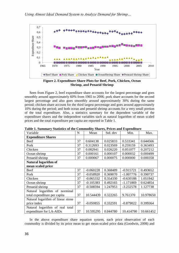
Figure 2. Expenditure Share Plots for Beef, Pork, Chicken, Ocean

Shrimp, and Penaeid Shrimp

Seen from Figure 2, beef expenditure share accounts for the largest percentage and goes

smoothly around approximately 60% from 1965 to 2006; pork share accounts for the second

largest percentage and also goes smoothly around approximately 30% during the same

period; chicken share account for the third largest percentage and goes around approximately

10% during the period; and both ocean and penaeid shrimp accounts for a very small portion

of the total expenditure. Also, a statistics summary for the dependent variable of the

expenditure shares and the independent variables such as natural logarithm of mean scaled

prices and the total expenditure per capita are reported in Table 1.

Table 1. Summary Statistics of the Commodity Shares, Prices and Expenditure

Variable N Mean Std. dev Min. Max.

Expenditure Shares

Beef 37 0.604138 0.025833 0.533341 0.644566

Pork 37 0.312693 0.023569 0.259159 0.363493

Chicken 37 0.082941 0.026220 0.051077 0.207212

Ocean shrimp 37 0.000161 0.000107 0.000032 0.000499

Penaeid shrimp 37 0.000067 0.000075 0.000000 0.000358

Natural logarithm of

mean scaled price

Beef 37 -0.060228 0.368489 -0.915721 0.493652

Pork 37 -0.058920 0.369070 -1.007776 0.390737

Chicken 37 -0.065332 0.354330 -0.630188 1.051942

Ocean shrimp 37 -0.105383 0.492165 -1.171869 0.624854

Penaeid shrimp 37 -0.508594 1.247953 -3.232578 1.127738

Natural logarithm of norminal

total expenditure per capita 37 10.544439 0.322265 9.761370 10.978650

Natural logarithm of linear stone

price index 37 -0.050855 0.332591 -0.879022 0.399364

Natural logarithm of real total

expenditure for LA-AIDs 37 10.595295 0.044780 10.414790 10.661452

In the above expenditure share equation system, each price observation of each

commodity is divided by its price mean to get mean-scaled price data (Goodwin, 2008) and

0

0,1

0,2

0,3

0,4

0,5

0,6

0,7

1965 1970 1975 1980 1985 1990 1995 2000 2005 2010

Exp

end

itu

re S

har

e

Year

Beef Share Pork Share Chicken Share OceanShrimp Share Peneaid Shrimp Share

X. Zhou

37

then is taken in natural log. Since the expenditure shares sum to 1 in the equation system,

one of the share equations is deleted to avoid the singularity and whichever one is eliminated

does not have any impact on the results (Goodwin, 2008). Thus, chicken expenditure share

equation is deleted and the parameters associated with the chicken share equation can be

calculated by the restrictions of both homogeneity and symmetry. Therefore the constant

coefficient in the chicken share equation can be obtained by subtracting the summation of the

other four constant coefficients from one. Similarly, the slope coefficient in the chicken share

equation can be calculated by subtracting the summation of the other four slope coefficients

from zero.

The nonlinear AIDs model was estimated by applying the MODEL procedure and the

econometric method of ITSUR (iterated seemingly unrelated regression) in SAS computer

program (Goodwin, 2008). The LA-AIDs model was estimated by applying the SYSLIN

procedure and the econometric method of ITSUR (Goodwin, 2008) in SAS computer

program, too. The parametric constraints of homogeneity and symmetry conditions were

imposed.

Once the AIDs model was estimated, the mean values of the uncompensated demand

elasticity, the compensated demand elasticity, and the expenditure elasticity would be

calculated for nonlinear AIDs and LA-AIDs estimates, respectively by the formulae

mentioned in the section of Theoretical Model, the average expenditure share, the average

logarithm price of each commodity, and the average real total expenditure.

4. Results

Table 2 presents the R2 for the system of equations from both nonlinear AIDs and LA-

AIDs estimation. Most of the R2s or adjusted R

2s are reasonable except the R

2 for the ocean

shrimp share equation from the nonlinear AIDs is extremely low to 6 or 7 percent in

magnitude. The reason could be the ocean shrimp accounts for a small percentage of the

total expenditure or data limitation. The system weighted R2 from LA-AIDs is much higher

than those from nonlinear AIDs. The reason could be different estimate procedure: SYSLIN

procedure is used in LA estimation and MODEL procedure is used in nonlinear estimation.

Table 2. R2 of ITSUR Estimation from Nonlinear AIDs and LA-AIDs Estimation

Nonlinear AIDs LA-AIDs

Beef

Share

Pork

Share

Chicken Share

Ocean Shrimp

Share

Penaeid Shrimp

Share

System

Weighted R2

R2 0.6643 0.7877 - 0.0627 0.4092 0.8962

Adj. R2 0.6163 0.7574 - -0.0712 0.3248

Table 3 presents the parameter estimates and associated standard error and P value of the

expenditure share function systems from nonlinear AIDs model and LA-AIDs model,

respectively. For the beef share equation, both nonlinear and LA intercept estimates are

positive and significant. The total expenditure coefficient estimate from nonlinear is

negative and significant, but the expenditure coefficient estimate from LA is positive and

insignificant. This implies that as the real total expenditure increases, nonlinear estimate

shows the beef expenditure share would decrease but the LA estimate shows the beef share

would not be correlated to the total expenditure. Both nonlinear and LA beef own price

coefficient estimates are significant. The nonlinear beef own price coefficient estimate is

negative as expected due to the downward own-price-demand curve theory, but the LA

estimate is positive. Also, the magnitude from LA estimate is much lower than that from the

nonlinear estimate. The reason could be correlation or data limitation.

Using Almost Ideal Demand System to Analyze Demand for Shrimp…

38

Table 3. ITSUR Parameter Estimates from the Nonlinear AIDs and LA-AIDs Models

Nonlinear AIDs LA-AIDs

Estimate Std. Error P-Value Estimate Std. Error P-Value

αb 8.14580 * 0.94620 <.0001 6.98378 * 1.27278 <.0001

αp -0.06631 0.77480 0.93230 -1.96659 0.99411 0.05750

αc -7.08322 * 0.54040 <.0001 -4.01684

αso -0.00266 0.00697 0.70470 0.00624 0.01033 0.55020

αsp 0.00641 0.00457 0.17130 -0.00659 0.00699 0.35330

βb -0.08456 * 0.01150 <.0001 0.06476 0.06494 0.32690

βp 0.00444 0.00942 0.64110 0.07933 0.04821 0.11070

βc 0.08003 -0.14415

βso 0.00005 0.00009 0.55870 -0.00027 0.00041 0.51730

βsp 0.00004 0.00009 0.62800 0.00032 0.00027 0.23900

γbb -0.58262 * 0.14860 0.00050 0.05458 * 0.02321 0.02570

γbp 0.01679 0.07960 0.83440 -0.00191 0.01968 0.92330

γbc 0.55926 * 0.07560 <.0001 -0.05224 * 0.00838 <.0001

γbso 0.00012 0.00064 0.84930 -0.00029 * 0.00017 0.09890

γbsp 0.00645 * 0.00267 0.02210 -0.00014 0.00012 0.24950

γpp 0.04480 * 0.02560 0.09000 0.02516 0.01984 0.21490

γpc -0.06821 0.06340 0.29000 -0.02348 * 0.00665 0.00140

γpso 0.00018 0.00010 0.08770 0.00009 0.00019 0.63100

γpsp 0.00104 0.00193 0.59400 0.00014 0.00013 0.28720

γcc -0.44396 * 0.03170 <.0001 0.07566

γcso -0.00031 0.00063 0.62480 0.00004 0.00007 0.58320

γcsp -0.04678 * 0.01780 0.01340 0.00002 0.00004 0.58920

γsoso 0.00002 0.00002 0.38830 0.00013 * 0.00004 0.00500

γsosp -0.00001 0.00001 0.58190 0.00003 * 0.00002 0.09540

γspsp 0.03930 * 0.01690 0.02660 -0.00006 * 0.00002 0.00090

λb -0.00334 * 0.00045 <.0001 -0.00355 * 0.00045 <.0001

λp 0.00017 0.00034 0.62710 0.00072 * 0.00035 0.04590

λc 0.00318 0.00283

λsoso 0.00000 0.00000 0.74670 0.00000 0.00000 0.66900

λsosp 0.00000 0.00000 0.15980 0.00000 0.00000 0.54000

Note: * denotes significance at the 0.10 level, based on asymptotic t-ratios.

X. Zhou

39

Both nonlinear and LA chicken price coefficient estimates are significant; the nonlinear

estimate is positive as expected, which implies that beef and chicken are strong substitute

commodities, but the LA estimate is negative; and the magnitude from LA estimate is much

lower than that from the nonlinear estimate, too. Correlation or data limitation might be the

reason to this difference or inconsistency, too. The pork price coefficient estimates have a

positive sign for nonlinear and negative sign for LA, and both are insignificant, which is

inconsistent with substitute commodity theory. Also, the magnitude from nonlinear is much

higher than that from LA. The reason could be beef and pork is not strong substitute

commodities, correlation or limited data constraints. Both nonlinear and LA ocean shrimp

price coefficient estimates are positive as expected, but nonlinear estimate is insignificant

and LA estimate is significant. Also, both estimates are small in magnitude. These might be

due to the small percentage of ocean shrimp expenditure share or data limitation. The same

issues happen to the penaeid shrimp price coefficient estimate.

For the pork share equation, the total expenditure coefficient estimates from both

nonlinear and LA are positive and insignificant. The insignificancy shows the pork share is

uncorrelated with the real total expenditure. This implies that the pork share would not

change as the real total expenditure change. Both nonlinear and LA pork own price

coefficient estimates are positive, which is contradictory to the downward own-price-demand

curve theory and indicates by theory that pork could be a Giffen good in the US market from

1970 to 2006. However, pork is not a Giffen good in the real market. The reason could be

correlation or data limitation. Beef price coefficient estimates are the same situation as the

pork price coefficient estimates in the beef share equation due to the symmetry. The chicken

price coefficient estimates from both nonlinear and LA is negative, and nonlinear estimate is

insignificant but LA is significant. This indicates that pork and chicken might be weak

complements in the US market from 1970 to 2006. The Ocean shrimp price coefficient

estimates from both nonlinear and LA is positive, and the nonlinear estimate is significant

but the LA is insignificant. The positive sign is consistent with the substitute commodity

theory. The penaeid shrimp price coefficient estimates from both nonlinear and LA is

positive, too but insignificant.

For the chicken share equation, the coefficient estimates of the real total expenditure and

the LA own price are calculated from symmetry and homogeneity already mentioned in the

section of Data and Method. The real total expenditure coefficient estimate from nonlinear is

positive, but the expenditure estimate from LA is negative. This implies that as the real total

expenditure increases, nonlinear estimate shows the chicken expenditure share would

increase, but the LA estimates shows that the chicken share would decrease. The chicken

own price coefficient estimate from nonlinear is negative and significant, which is consistent

with the downward own-price-demand curve theory; but the estimate from LA is positive,

which is calculated from symmetry and homogeneity. The reason could be different

estimations procedures mentioned in the section of Data and Method. The beef price

coefficient estimates are the same as the chicken price coefficient estimates in the beef share

equation due to the symmetry. Likely, the pork price coefficient estimates are the same as

the chicken price coefficient in the pork share equation due to the symmetry. Also, the ocean

shrimp price coefficient estimates are the same as the chicken price coefficient estimates in

the ocean shrimp share equation and the penaeid shrimp price coefficient estimates are the

same as the chicken price coefficient estimates in the penaeid shrimp share equation, which

will be discussed as follows.

For the ocean shrimp share equation, the total expenditure coefficient estimate from

nonlinear is positive, but the estimate from LA is negative. Both estimates are insignificant

and small in magnitude. The ocean shrimp own price coefficient estimates from both

nonlinear and LA are positive and small in magnitude. The estimate from nonlinear is

insignificant, but the estimate from LA is significant. The positive sign is contradictory to

Using Almost Ideal Demand System to Analyze Demand for Shrimp…

40

the downward own-price-demand curve theory. The reason could be correlation or data

limitation. The beef price coefficient estimates and pork price coefficients estimates are the

same as those in the beef share equation and pork share equation due to the symmetry. The

chicken price coefficient estimate from nonlinear is negative, but estimate from LA is

positive. Both estimates are insignificant and small to the fourth or fifth decimal digit in

magnitude. Both nonlinear and LA pork price coefficient estimates are positive and small to

the fourth or fifth decimal digit in magnitude. The nonlinear estimate is significant, but LA

estimate is insignificant. The penaeid shrimp price coefficient estimate from nonlinear is

negative and insignificant, but the estimate from LA is positive and significant. Estimates

from both nonlinear and LA are small to the fifth decimal digit in magnitude.

For the penaeid shrimp share equation, the total expenditure coefficient estimates from

both nonlinear and LA are positive, insignificant, and small to the fourth or fifth decimal

digits. The penaeid shrimp own price coefficient estimate from nonlinear is positive which is

contradictory to the downward own-price-demand curve theory; but the estimate from LA is

negative and much smaller than nonlinear estimate in magnitude. Both own price coefficient

estimates are significant. The beef price coefficient estimates and pork price coefficients

estimates are the same as those in the beef share equation and pork share equation due to the

symmetry. The chicken price coefficient estimate from nonlinear is negative and significant,

but the estimate from LA is positive and insignificant. LA estimate is much lower than

nonlinear estimate in magnitude. The ocean shrimp price coefficient estimates are the same

as the penaeid shrimp price coefficients in the ocean shrimp share equation due to the

symmetry.

The year trend coefficient estimates from both nonlinear and LA are consistent. The year

estimates from share equations of pork, chicken, ocean shrimp, and penaeid shrimp are

positive, insignificant, and small to third or fifth decimal digits in magnitude. This implies

that time trend is not correlated to the expenditure share. Estimates of beef share equations

from both nonlinear and LA are negative and significant, which indicates that as time goes

by, beef share would be decreased little by little.

In comparison, there are quite a few differences for the coefficient estimates of total

expenditure and price between nonlinear AIDs and LA-AIDs in terms of sign, magnitude,

and statistical significance (Figures 3 and 4). The reason could be different estimate

procedure: MODEL procedure for nonlinear AIDs and the SYSLIN procedure for LA-AIDs

or some other reasons that need to be further studied.

Figure 3. Compare Price Coefficient Estimates from Nonlinear AIDs and

LA-AIDs

-0,8

-0,6

-0,4

-0,2

0,0

0,2

0,4

0,6

0,8

γbb γbp γbc γbso γbsp γpp γpc γpso γpsp γcc γcso γcsp γsoso γsosp γspsp Est

imat

es

Coefficient

Nonlinear AIDs Estimates LA-AIDs Estimates

X. Zhou

41

Figure 4. Compare Total Expenditure Coefficient Estimates from

Nonlinear AIDs and LA-AIDs

Given the coefficient estimates of total expenditure and prices, the mean values of

expenditure elasticity, uncompensated demand elasticity, and compensated demand elasticity

were calculated by the formulae mentioned in the section of Data and Method. Tables 4, 5,

and 6 present these results. Seen from Table 4 and Figure 5, the mean values of beef and

pork expenditure elasticity from nonlinear AIDs is slightly smaller than that from LA; the

mean value of beef expenditure elasticity is close to 1 from LA and nonlinear, so is the mean

value of pork. This indicates that a 1 percent increase in the total expenditure would induce

an approximately 1 percent increase in quantity demanded for both beef and pork. However,

the mean values of chicken, ocean and penaeid shrimp expenditure elasticity from nonlinear

are much higher than that from LA. Their mean values of expenditure elasticity from

nonlinear are greater than 1, which implies that a 1 percent increase in total expenditure

would induce more than 1 percent increase in the quantity demanded for the three

commodities; but the mean values of chicken and ocean shrimp expenditure elasticity from

LA is less than 1, which implies that that a 1 percent increase in total expenditure would

induce less than 1 percent increase in the quantity demanded. Therefore, the mean values of

beef and pork expenditure elasticity from nonlinear are consistent with those from LA; but

the mean values of chicken, ocean shrimp, and penaeid shrimp elasticity from nonlinear are

inconsistent with those from LA: nonlinear shows more sensitive consumer demand to

expenditure, but LA shows much less sensitive consumer demand to expenditure. In general,

the consumption for each of the five goods would increase by approximately 1 percent as the

real total expenditure increase by 1 percent.

Table 4. Mean Values of Expenditure Elasticity from both

LA-AIDs and Nonlinear AIDs Models

Expenditure Elasticity

LA - AIDs Nonlinear AIDs

Beef 1.05303 0.8600261

Pork 1.06496 1.0141908

Chicken 0.88196 1.9649423

Ocean Shrimp 0.99978 1.3231964

Penaeid Shrimp 1.00026 1.6376027

-0,20

-0,15

-0,10

-0,05

0,00

0,05

0,10

βb βp βc βso βsp

Est

imat

es

Coefficient

Nonlinear AIDs Estimates LA-AIDs Estimates

Using Almost Ideal Demand System to Analyze Demand for Shrimp…

42

Figure 5. Compare Mean Values of Expenditure Elasticity from

LA-AIDs and Nonlinear AIDs

Table 5 and Figure 6 present the mean values of uncompensated demand elasticity matrix

from both LA-AIDs and nonlinear AIDs model. The mean values of estimated own-price

elasticities from LA-AIDs are negative for the five commodities, which is consistent to

downward own-price demand curve theory. The magnitude is less than 1 except for the

penaeid shrimp. The magnitude for beef and pork is close to 1 and magnitude for chicken

and ocean shrimp is close to 0.1 and 0.3, which implies consumer’s demand for beef and

pork is much more responsive with respective to price than for chicken and ocean shrimp.

The highest magnitude is 1.7 for penaeid shrimp. This indicates that among the five

commodities, consumer’s demand for penaeid shrimp is the most responsive with respect to

its own price. The mean values of estimated cross-price elasticity from LA-AIDs are not

symmetric in terms of sign. This is implausible probably due to the statistical insignificance.

The negative sign implies complementary commodities for beef-pork, beef-chicken, beef-

ocean shrimp, etc., and the positive sign implies the substitute commodities for the rest pairs.

Table 5. Mean Values of Uncompensated Demand Elasticity from both LA-AIDs and

Nonlinear AIDs Models

Beef Pork Chicken Ocean Shrimp Penaeid Shrimp

LA -AIDs

Beef -0.97905 -0.03004 -0.07809 -0.00041 -0.00020

Pork -0.13052 -0.99908 -0.07872 0.00021 0.00035

Chicken 0.34403 0.21318 -0.13496 0.00059 0.00033

Ocean Shrimp -0.64939 0.91320 0.30398 -0.34467 0.17411

Penaeid Shrimp -4.11768 0.47919 -0.03427 0.41711 -1.73746

Nonlinear AIDs

Beef -1.75473 0.06500 0.81893 0.00015 0.01061

Pork 0.03245 -0.86051 -0.20731 0.00057 0.00334

Chicken 5.29764 -1.07887 -5.61669 -0.00337 -0.56367

Ocean Shrimp 0.28608 1.01410 -1.69173 -0.88250 -0.04914

Penaeid Shrimp 95.74295 15.45459 -701.41280 -0.11803 588.69572

0

0,5

1

1,5

2

2,5

Beef Pork Chicken Ocean Shrimp Penaeid Shrimp

Ela

scit

icit

y

LA-AIDs Nonlinear AIDs

X. Zhou

43

Figure 6. Mean Values of Uncompensated Elasticity from LA-AIDs and Nonlinear

AIDs, respectively

The mean values of the estimated own price elasticity from nonlinear are negative except

penaeid shrimp. Also, the magnitude for penaeid shrimp is unreasonably high. The reason

could be data limitation or statistical insignificance. The highest magnitude implies that

consumer’s demand for penaeid shrimp is the most sensitive to its own price among the five

commodities. Chicken own price elasticity is the highest in magnitude except penaeid

shrimp, beef is the second highest, ocean shrimp is the third, and pork follows closely. The

mean values of estimated cross-price elasticity from nonlinear are symmetric in terms of

sign. The positive sign indicates the substitute commodity pairs which are beef-pork, beef-

chicken, beef-ocean shrimp, beef-penaeid shrimp, pork-ocean shrimp, and pork penaeid

shrimp. Also, the negative sign indicates the complementary commodity pairs which are the

rest.

In comparison, the mean values of the uncompensated demand elasticity from LA-AIDs

estimates are consistent with those from nonlinear in terms of the negative sign of the own-

price elasticity except penaeid shrimp. However, both are inconsistent in terms of cross-

price elasticity. The mean values of the uncompensated cross-price elasticities from

nonlinear are symmetric in terms of sign, which is reasonable; but the mean values of the

uncompensated cross-price elasticity from LA are not symmetric in terms of sign, which is

unreasonable. The reason could be the different estimation procedure or statistical

insignificance.

Table 6 and Figure 7 present mean values of compensated demand elasticity from LA-

AIDs and nonlinear AIDs respectively. For the mean values of compensated elasticity from

LA-AIDs, all the mean values of own-price elasticity are negative, but ocean shrimp and

penaeid shrimp are unreasonably large in magnitude. Most of the mean values of cross-price

elasticity from LA-AIDs are symmetric in terms of sign except that chicken-beef is positive,

but beef-chicken is negative. Also, ocean shrimp pairs and penaeid shrimp pairs are

unreasonably high in magnitude. The reason could be the small percentage expenditure

share. For the mean values of compensated elasticity from nonlinear AIDs, all the mean

values of own-price elasticity are negative and reasonable in magnitude except penaeid

shrimp is positive and unreasonable in magnitude. All the mean values of cross-price

elasticity from nonlinear AIDs are symmetric in terms of sign. Three pairs such as penaeid

shrimp-beef, penaeid shrimp-chicken, and penaeid shrimp own are unreasonably high in

magnitude.

BeefPork

ChickenOcean ShrimpPenaeid Shrimp

-5

-4

-3

-2

-1

0

1B

eef

Po

rk

Chic

ken

Oce

an S

hri

mp

Pen

aeid

Shri

mp

Uncompensated Elasticity from LA-AIDs

Beef PorkChicken Ocean ShrimpPenaeid Shrimp

BeefPork

ChickenOcean ShrimpPanaeid Shrimp

-5

-4

-3

-2

-1

0

1

Bee

f

Po

rk

Chic

ken

Oce

an S

hri

mp

Pen

aeid

Shri

mp

Uncompensated Elasticity from Nonlinear

AIDs

Beef Pork

Chicken Ocean Shrimp

Panaeid Shrimp

Using Almost Ideal Demand System to Analyze Demand for Shrimp…

44

Table 6. Mean Values of Compensated Demand Elasticity from LA-AIDs and

Nonlinear AIDs models, respectively

Beef Pork Chicken

Ocean

Shrimp

Penaeid

Shrimp

LA - AIDs

Beef -2.01643 0.26297 -0.04632 -0.00051 -0.00026

Pork 0.18674 -3.88243 -0.16882 0.00084 0.00119

Chicken 4.75205 2.88303 -2.54425 0.00731 0.00407

Ocean Shrimp -4058.08142 5707.78189 1899.96140 -2155.17641 1088.16173

Penaeid Shrimp -61780.7542 7190.03274 -514.17362 6258.25260 -26069.68681

Nonlinear AIDs

Beef -1.23515 0.33392 0.89027 0.00029 0.01067

Pork 0.64516 -0.54339 -0.12319 0.00073 0.00340

Chicken 6.48474 -0.46445 -5.45371 -0.00305 -0.56354

Ocean Shrimp 1.08548 1.42785 -1.58198 -0.88229 -0.04906

Penaeid Shrimp 96.73230 15.96665 -701.27700 -0.11776 588.69583

By comparison of results from LA-AIDs and nonlinear AIDs, there are quite a few

differences between them. Results from nonlinear AIDs are more expected and more

complied with microeconomic theory than those from LA-AIDs. For example, the mean

values of uncompensated and compensated elasticities from nonlinear AIDs are symmetric,

but those from LA-AIDs are not symmetric; the nonlinear beef own price coefficient

estimate is negative as expected due to the downward own-price-demand curve theory, but

the LA estimate is positive; and the magnitude from LA estimate is much lower than that

from the nonlinear estimate.

Figure 7. Mean Values of Compensated Elasticity from LA-AIDs and Nonlinear AIDs,

respectively

BeefPork

ChickenOcean shrimp

Penaeid shrimp

-5

-4

-3

-2

-1

0

1

Compensated Demand Elasciticity from

LA-AIDs

Beef PorkChicken Ocean shrimpPenaeid shrimp

BeefPork

ChickenOcean shrimpPenaeid shrimp

-5

-4

-3

-2

-1

0

1

Compensated Demand Elasciticity from

Nonlinear AIDs

Beef Pork

Chicken Ocean shrimp

Penaeid shrimp

X. Zhou

45

5. Conclusions

This paper uses both models of nonlinear AIDs and LA-AIDs to examine the demand

system analysis of beef, pork, chicken, ocean shrimp, and penaeid shrimp in the U.S. food

market, especially focusing on the own and cross relationship between the expenditure share

and price, expenditure changes from the above five food commodities. Mean Values of the

expenditure elasticity, compensated and uncompensated elasticity are calculated to imply the

consumer’s demand responsiveness with respective to the change of the expenditure, own

price, and cross price. These results contribute much to predicting supply strategies,

consumer preferences and policy making.

Results from nonlinear AIDs model is compared with those from LA-AIDs model. There

are quite a few inconsistency between nonlinear and LA results. Results from nonlinear are

more expected and more complied with microeconomic theory than those from LA. Further

study needs to be conducted on whether nonlinear AIDs model is more valid than LA-AIDs

in the application of food demand analysis.

Empirical results indicated that some insignificant slope coefficients and inappropriate

signs of them did not comply with microeconomic theory. This could be caused by

heteroscedasticity, autocorrelation, a limitation in the data used, too few years of data or

shrimp is a commodity that is quite different. Further investigation into our data and demand

elasticities is being conducted.

6. References

Adams, C., Prochaska, F. & Spreen, T. (1987). Price determination in the US shrimp market.

Southern Journal of Agricultural Economics 9, 103-112.

Asche, F. & Wessells, C.R. (1997). On price indices in the Almost Ideal Demand System.

American Journal of Agricultural Economics 79, 1182-1185.

Dahlgran, R.A. (1987). Complete flexibility systems and the stationarity of U.S. meat

demands. Western Journal of Agricultural Economics 12 (2), 152-163.

Davis, C. G. and Lin, B. H. (2005). Factors affecting U.S. pork consumption. United States

Department of Agriculture, (LDP-M-130-01).

Deaton, A. & Muellbauer J. (1980). An Almost Ideal Demand System. The American

Economic Review 70, 312 – 326.

Dey, M.M. (2000). Analysis of demand for fish in Bangladesh. Aquaculture Economics and

Management 4, 65 – 83.

Doll, J. (1972). An econometric analysis of shrimp ex-vessel prices. American Journal of

Agricultural Economics 54, 431-440.

Edgerton, D.L., Assarsson, B., Hummelmose, A., Laurila, I.P., Rickertsen, K., & Vale, P.H.

(1996). The econometrics of demand systems with applications to food demand in the

Nordic countries. Kluwer Academic Publishers.

Fisher, D., Fleissig, A.R., & Serletis, A. (2001). An empirical comparison of flexible demand

system functional forms. Journal of Applied Econometrics 16, 59-80.

Goodwin, B. (2008). SAS/ETS examples: Estimating an Almost Ideal Demand System

model. Available at http://support.sas.com/rnd/app/examples/ets/aids/.

Goodwin, B. (2008). SAS/ETS examples: Calculating elasticities in an Almost Ideal Demand

System model. Available at http://support.sas.com/rnd/app/examples/ets/elasticity/.

Green, R. & Alston, J.M. (1991). Elasticities in AIDs models: A clarification and extension.

American Journal of Agricultural Economics 73, 874-875.

Haby, M.G. (2003). Status of the world and U.S. shrimp markets. Trade Adjustment

Assistance for Farmers Technical Assistance, United States Department of Agriculture

(pp. 7-23).

Using Almost Ideal Demand System to Analyze Demand for Shrimp…

46

Haley, M.M. (2001). Changing consumer demand for meat: the U.S. example, 1970-2000.

Economic Research Service, United States Department of Agriculture.

Heien, D. & Pompelli, G. (1988). The demand for beef products: cross-section estimation of

demographic and economic effects. Western Journal of Agricultural Economics 13, 37-

44.

Houston, J.E & Li, H.S. (2000). Factors affecting consumer preferences for shrimp in

Taiwan. Department of Agricultural and Applied Economics, University of Georgia and

Food Industry Research and Development Institute, Taiwan.

Huang, K.S. & Lin, B.H. (2000). Estimation of food demand and nutrient elasticities from

household survey data. Economic Research service, U.S. Department of Agriculture, (TB

– 1887).

United States Department of Agriculture (USDA). (2005). Livestock & Meat Domestic Data.

Available at http://www.ers.usda.gov/data-products/livestock-meat-domestic-data.aspx.

United States Department of Commerce (USDOC). (2005). Per Capita Consumption.

Available at http:// http://www.st.nmfs.noaa.gov/st1/fus/fus05/08_perita2005.pdf.