Dynamic Almost Ideal Demand Systems:

An Empirical Analysis of Alcohol Expenditure in Ireland

John M. Eakins Economic and Social Research Institute, Ireland

Liam A. Gallagher University College Cork, Ireland

and

Dublin City University, Ireland

Current Draft: January 2003

Final Paper: Liam A. Gallagher John E. Eakins. 2003. Dynamic Almost Ideal Demand

Systems: An Empirical Analysis of Alcohol Expenditure in Ireland. Applied

Economics, 35(9), pp1025-1036.

Abstract

This paper presents a dynamic form of the Almost Ideal Demand System (AIDS). We employ three

versions of the static AIDS model to determine the preferred long-run equilibrium model and

represents the short-run dynamics by an error correction mechanism. This estimation procedure is

then applied to alcohol expenditure in Ireland. The estimated point elasticities are consistent with

previous studies and a priori expectations. Beer and spirits are found to be price inelastic in both the

short and long run. While wine is price inelastic in the short run and price elastic in the long run.

JEL Classification: D0

Keywords: AIDS, elasticity, alcohol, dynamic modelling

Correspondence:

Liam A. Gallagher

Business School

Dublin City University

Dublin 9

Ireland

Tel: + 353 1 7005399

Email: Liam.Gallagher@dcu.ie

1

Dynamic Almost Ideal Demand Systems:

An Empirical Analysis of Alcohol Expenditure in Ireland Abstract: This paper presents a dynamic form of the Almost Identical Demand System

(AIDS). We employ three versions of the AIDS model to determine the preferred long-run

equilibrium model to use in a dynamic specification, that has similar characteristics to an

error correction mechanism. This estimation procedure is applied to the demand for alcohol

in Ireland. Beer is found to be price inelastic in both the short and long run. Spirits is price

elastic in the short run and price inelastic in the long run. Wine is price elastic in the both the

short and long run.

I Introduction

The interest in modelling demand systems has increased with the availability of

longer horizon databases and advancements in econometric methodology. The Almost Ideal

Demand System (AIDS), developed by Deaton and Muellbauer (1980), remains the most

popular specification over the last 20 years. However, a feature of previous demand studies is

that the point elasticity estimates are not robust to the estimation period. In particular, it

appears that the short-run elasticity estimates substantially differ from their long-run values.

It is this characteristic that we explore in this paper in the context of the demand for alcohol in

Ireland for the period 1960-1998. We estimate price and expenditure (income) elasticities for

three different categories of alcohol: beer, spirits and wine. Employing a dynamic demand

system modelling approach, these elasticities are estimated for both short run and long run.

The application of this dynamic AIDS model to alcohol demand is of particular

importance to the drinks industry and to the Irish economy in general. In 1998, around €4.13

billion was spent on alcohol products alone. This constituted around 10% of total personal

expenditure in Ireland for that year. In terms of employment, Conniffe and McCoy (1993)

estimated that in 1990 some 33,000 full-time equivalent people were employed in the alcohol

industry. Foley (1999) showed that this figure had increased to over 43,000 persons by 1998.

Also, in 1998, the government collected in excise duty some €748 million; €465 million from

beer sales, €188 million from spirits and €95 million from wine. As a percentage of

government's total net receipts, beer was 2.3%, spirits was 0.9% and wine was 0.4%.

Furthermore, the total tax content on a pint of beer in 1998 was 35.6% of the price and for a

glass of spirits it was 35.5% of the price (Revenue Commissioners, Statistical Report 1998).

Analysis of alcohol use in Ireland, particularly in relation to estimation of elasticities is of

particular importance to both the alcohol industry (in the form of production and pricing

policies) and the government (in the collection of revenue).

2

This paper contributes to the existing literature in two ways. First, with the exception

of Walsh and Walsh (1970), Thom (1984) and Conniffe and McCoy (1993) there has been no

substantive economic analysis of the demand for alcoholic beverages in Ireland. Employing

more recent econometric techniques and a longer database, the robustness of previous studies

is investigated. Second, we advance previous methodology that is employed in estimating

demand systems using time series data. We modify the standard Almost Ideal Demand

System (AIDS) developed by Deaton and Muellbauer (1980) by representing demand as a

dynamic data generating process (DGP) that allows the use of time series information to

estimate short- and long-run elasticities. We apply this methodology to estimate the demand

elasticities for individual alcoholic drinks in Ireland. The dynamic AIDS representation is of

an error correction1 form of the AIDS model, that models the disequilibrium separate from the

AIDS long-run equilibrium and thus gives the short-run relationship between the demand

variables.

The remainder of the paper is set out as follows. In Section II we discuss the static

and dynamic AIDS modelling in estimating elasticities. This section also contains a short

review of recent empirical evidence. The data is outlined in Section III. Section IV

investigates the time series properties of the relevant data and provides the econometric

estimation, including the calculation of long run elasticity measures and tests for the dynamic

AIDS. Section V presents the dynamic AIDS results. A final section concludes.

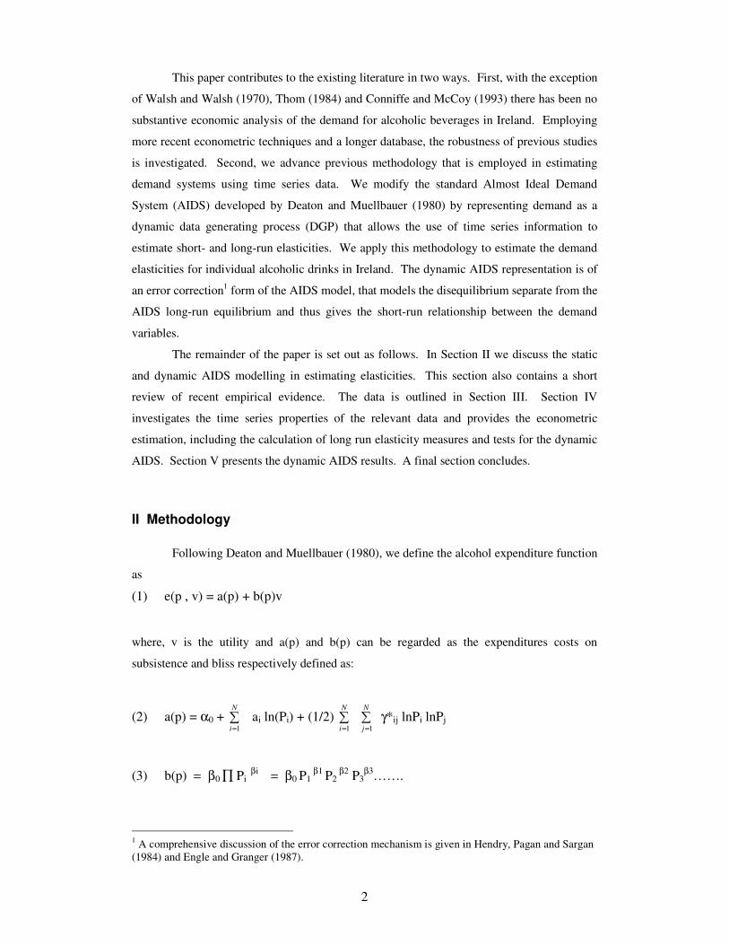
II Methodology

Following Deaton and Muellbauer (1980), we define the alcohol expenditure function

as

(1) e(p , v) = a(p) + b(p)v

where, v is the utility and a(p) and b(p) can be regarded as the expenditures costs on

subsistence and bliss respectively defined as:

(2) a(p) = α0 + ∑=

N

i 1

ai ln(Pi) + (1/2) ∑=

N

i 1

∑=

N

j 1

γ*ij lnPi lnPj

(3) b(p) = β0 ∏ Pi βi

= β0 P1 β1

P2 β2

P3β3

…….

1 A comprehensive discussion of the error correction mechanism is given in Hendry, Pagan and Sargan

(1984) and Engle and Granger (1987).

3

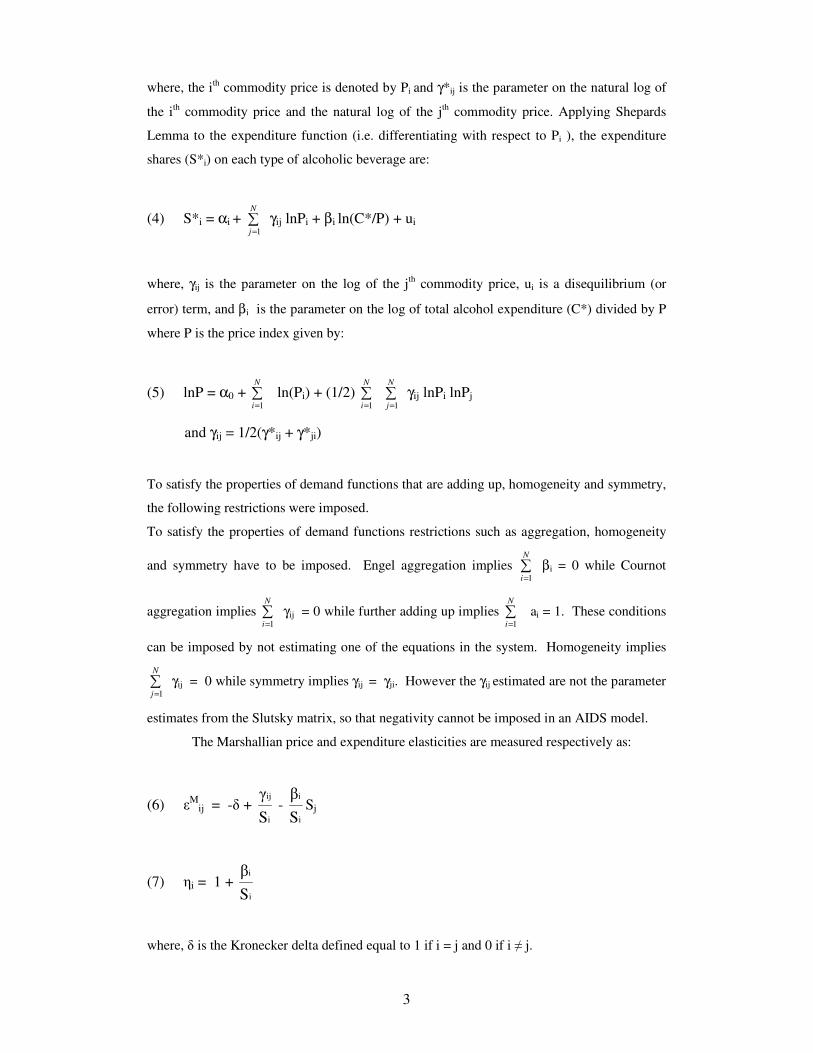
where, the ith commodity price is denoted by Pi and γ*ij is the parameter on the natural log of

the ith commodity price and the natural log of the jth commodity price. Applying Shepards

Lemma to the expenditure function (i.e. differentiating with respect to Pi ), the expenditure

shares (S*i) on each type of alcoholic beverage are:

(4) S*i = αi + ∑=

N

j 1

γij lnPi + βi ln(C*/P) + ui

where, γij is the parameter on the log of the jth commodity price, ui is a disequilibrium (or

error) term, and βi is the parameter on the log of total alcohol expenditure (C*) divided by P

where P is the price index given by:

(5) lnP = α0 + ∑=

N

i 1

ln(Pi) + (1/2) ∑=

N

i 1

∑=

N

j 1

γij lnPi lnPj

and γij = 1/2(γ*ij + γ*ji)

To satisfy the properties of demand functions that are adding up, homogeneity and symmetry,

the following restrictions were imposed.

To satisfy the properties of demand functions restrictions such as aggregation, homogeneity

and symmetry have to be imposed. Engel aggregation implies ∑=

N

i 1

βi = 0 while Cournot

aggregation implies ∑=

N

i 1

γij = 0 while further adding up implies ∑=

N

i 1

ai = 1. These conditions

can be imposed by not estimating one of the equations in the system. Homogeneity implies

∑=

N

j 1

γij = 0 while symmetry implies γij = γji. However the γij estimated are not the parameter

estimates from the Slutsky matrix, so that negativity cannot be imposed in an AIDS model.

The Marshallian price and expenditure elasticities are measured respectively as:

(6) εM

ij = -δ + i

ij

S

γ -

i

i

S

βSj

(7) ηi = 1 + i

i

S

β

where, δ is the Kronecker delta defined equal to 1 if i = j and 0 if i ≠ j.

4

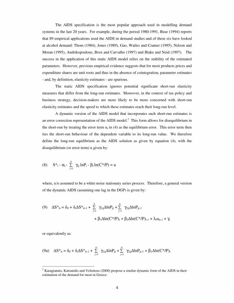
The AIDS specification is the most popular approach used in modelling demand

systems in the last 20 years. For example, during the period 1980-1991, Buse (1994) reports

that 89 empirical applications used the AIDS in demand studies and of these six have looked

at alcohol demand: Thom (1984), Jones (1989), Gao, Wailes and Cramer (1995), Nelson and

Moran (1995), Andrikopoulous, Brox and Carvalho (1997) and Blake and Neid (1997). The

success in the application of this static AIDS model relies on the stability of the estimated

parameters. However, previous empirical evidence suggests that for most products prices and

expenditure shares are unit roots and thus in the absence of cointegration, parameter estimates

- and, by definition, elasticity estimates - are spurious.

The static AIDS specification ignores potential significant short-run elasticity

measures that differ from the long-run estimates. Moreover, in the context of tax policy and

business strategy, decision-makers are more likely to be more concerned with short-run

elasticity estimates and the speed to which these estimates reach their long-run level.

A dynamic version of the AIDS model that incorporates such short-run estimates is

an error correction representation of the AIDS model.2 This form allows for disequilibrium in

the short-run by treating the error term ui in (4) as the equilibrium error. This error term then

ties the short-run behaviour of the dependent variable to its long-run value. We therefore

define the long-run equilibrium as the AIDS solution as given by equation (4), with the

disequilibrium (or error term) u given by:

(8) S*i - αi - ∑=

N

j 1

γij lnPi - βi ln(C*/P) = u

where, u is assumed to be a white noise stationary series process. Therefore, a general version

of the dynamic AIDS (assuming one lag in the DGP) is given by:

(9) ∆S*it = δ0 + δi∆S*it-1 + ∑=

N

j 1

γ1ij∆lnPjt +∑=

N

j 1

γ2ij∆lnPjt-1

+ β1∆ln(C*/P)t + β2∆ln(C*/P)t-1 + λiuit-1 + γt

or equivalently as:

(9a) ∆S*it = δ0 + δi∆S*it-1 + ∑=

N

j 1

γ1ij∆lnPjt + ∑=

N

j 1

γ2ij∆lnPjt-1 + β1∆ln(C*/P)t

2 Karagiannis, Katranidis and Velentzas (2000) propose a similar dynamic form of the AIDS in their

estimation of the demand for meat in Greece.

5

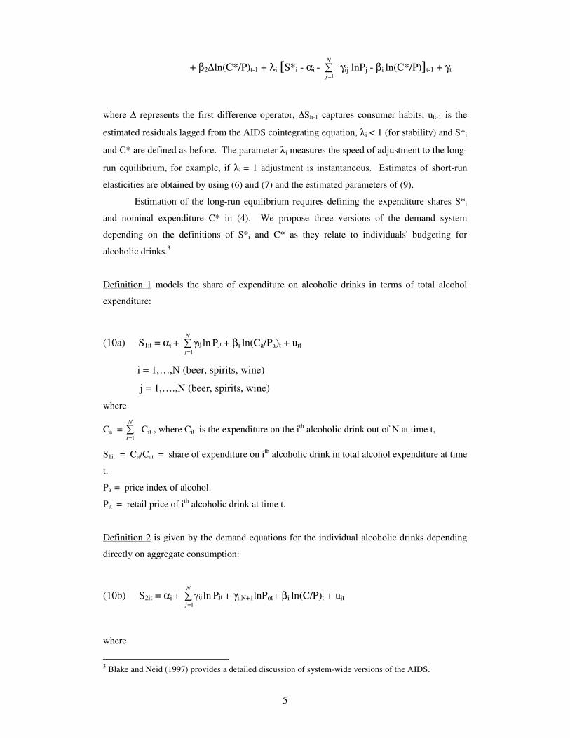
+ β2∆ln(C*/P)t-1 + λi [S*i - αi - ∑=

N

j 1

γij lnPj - βi ln(C*/P)]t-1 + γt

where ∆ represents the first difference operator, ∆Sit-1 captures consumer habits, uit-1 is the

estimated residuals lagged from the AIDS cointegrating equation, λi < 1 (for stability) and S*i

and C* are defined as before. The parameter λi measures the speed of adjustment to the long-

run equilibrium, for example, if λi = 1 adjustment is instantaneous. Estimates of short-run

elasticities are obtained by using (6) and (7) and the estimated parameters of (9).

Estimation of the long-run equilibrium requires defining the expenditure shares S*i

and nominal expenditure C* in (4). We propose three versions of the demand system

depending on the definitions of S*i and C* as they relate to individuals' budgeting for

alcoholic drinks.3

Definition 1 models the share of expenditure on alcoholic drinks in terms of total alcohol

expenditure:

(10a) S1it = αi + ∑=

N

j 1

jtij Plnγ + βi ln(Ca/Pa)t + uit

i = 1,…,N (beer, spirits, wine)

j = 1,….,N (beer, spirits, wine)

where

Ca = ∑=

N

i 1

Cit , where Cit is the expenditure on the ith alcoholic drink out of N at time t,

S1it = Cit/Cat = share of expenditure on ith alcoholic drink in total alcohol expenditure at time

t.

Pa = price index of alcohol.

Pit = retail price of ith alcoholic drink at time t.

Definition 2 is given by the demand equations for the individual alcoholic drinks depending

directly on aggregate consumption:

(10b) S2it = αi + ∑=

N

j 1

jtij Plnγ + γi,N+1lnPot+ βi ln(C/P)t + uit

where

3 Blake and Neid (1997) provides a detailed discussion of system-wide versions of the AIDS.

6

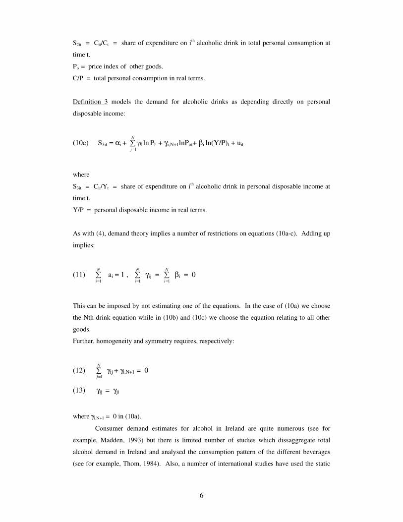
S2it = Cit/Ct = share of expenditure on ith alcoholic drink in total personal consumption at

time t.

Po = price index of other goods.

C/P = total personal consumption in real terms.

Definition 3 models the demand for alcoholic drinks as depending directly on personal

disposable income:

(10c) S3it = αi + ∑=

N

j 1

jtij Plnγ + γi,N+1lnPot+ βi ln(Y/P)t + uit

where

S3it = Cit/Yt = share of expenditure on ith alcoholic drink in personal disposable income at

time t.

Y/P = personal disposable income in real terms.

As with (4), demand theory implies a number of restrictions on equations (10a-c). Adding up

implies:

(11) ∑=

N

i 1

ai = 1 , ∑=

N

i 1

γij = ∑=

N

i 1

βi = 0

This can be imposed by not estimating one of the equations. In the case of (10a) we choose

the Nth drink equation while in (10b) and (10c) we choose the equation relating to all other

goods.

Further, homogeneity and symmetry requires, respectively:

(12) ∑=

N

j 1

γij + γi,N+1 = 0

(13) γij = γji

where γi,N+1 = 0 in (10a).

Consumer demand estimates for alcohol in Ireland are quite numerous (see for

example, Madden, 1993) but there is limited number of studies which dissaggregate total

alcohol demand in Ireland and analysed the consumption pattern of the different beverages

(see for example, Thom, 1984). Also, a number of international studies have used the static

7

AIDS specification (Jones, 1989; Nelson and Moran, 1995; Gao et al., 1995; Andrikopoulous,

Box and Carvalho, 1997). In contrast, Johnson, Oksanen, Veall and Fretz (1992) use an

unrestricted error correction mechanism (ECM) to estimate short-run and long-run elasticities

for Canadian alcohol data. However, unlike the other studies, Johnson et al. (1992)

methodology does not incorporate a theoretical underlying demand system model.

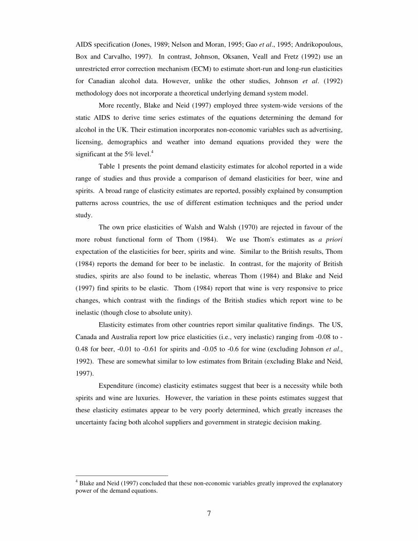
More recently, Blake and Neid (1997) employed three system-wide versions of the

static AIDS to derive time series estimates of the equations determining the demand for

alcohol in the UK. Their estimation incorporates non-economic variables such as advertising,

licensing, demographics and weather into demand equations provided they were the

significant at the 5% level.4

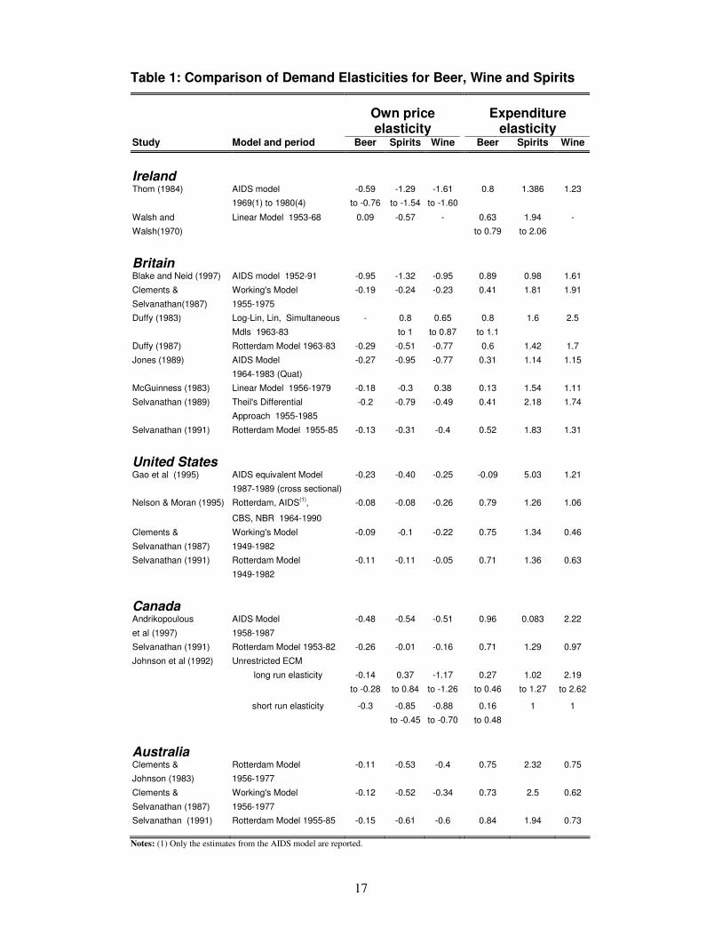
Table 1 presents the point demand elasticity estimates for alcohol reported in a wide

range of studies and thus provide a comparison of demand elasticities for beer, wine and

spirits. A broad range of elasticity estimates are reported, possibly explained by consumption

patterns across countries, the use of different estimation techniques and the period under

study.

The own price elasticities of Walsh and Walsh (1970) are rejected in favour of the

more robust functional form of Thom (1984). We use Thom's estimates as a priori

expectation of the elasticities for beer, spirits and wine. Similar to the British results, Thom

(1984) reports the demand for beer to be inelastic. In contrast, for the majority of British

studies, spirits are also found to be inelastic, whereas Thom (1984) and Blake and Neid

(1997) find spirits to be elastic. Thom (1984) report that wine is very responsive to price

changes, which contrast with the findings of the British studies which report wine to be

inelastic (though close to absolute unity).

Elasticity estimates from other countries report similar qualitative findings. The US,

Canada and Australia report low price elasticities (i.e., very inelastic) ranging from -0.08 to -

0.48 for beer, -0.01 to -0.61 for spirits and -0.05 to -0.6 for wine (excluding Johnson et al.,

1992). These are somewhat similar to low estimates from Britain (excluding Blake and Neid,

1997).

Expenditure (income) elasticity estimates suggest that beer is a necessity while both

spirits and wine are luxuries. However, the variation in these points estimates suggest that

these elasticity estimates appear to be very poorly determined, which greatly increases the

uncertainty facing both alcohol suppliers and government in strategic decision making.

4 Blake and Neid (1997) concluded that these non-economic variables greatly improved the explanatory

power of the demand equations.

8

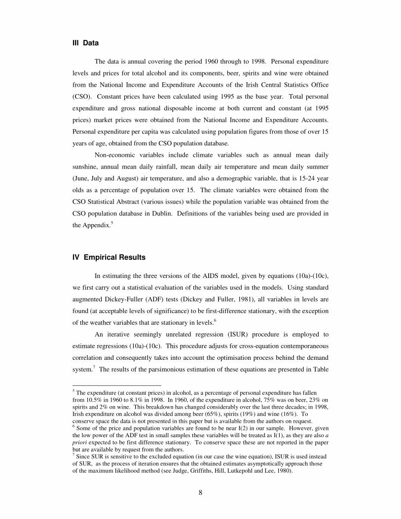
III Data

The data is annual covering the period 1960 through to 1998. Personal expenditure

levels and prices for total alcohol and its components, beer, spirits and wine were obtained

from the National Income and Expenditure Accounts of the Irish Central Statistics Office

(CSO). Constant prices have been calculated using 1995 as the base year. Total personal

expenditure and gross national disposable income at both current and constant (at 1995

prices) market prices were obtained from the National Income and Expenditure Accounts.

Personal expenditure per capita was calculated using population figures from those of over 15

years of age, obtained from the CSO population database.

Non-economic variables include climate variables such as annual mean daily

sunshine, annual mean daily rainfall, mean daily air temperature and mean daily summer

(June, July and August) air temperature, and also a demographic variable, that is 15-24 year

olds as a percentage of population over 15. The climate variables were obtained from the

CSO Statistical Abstract (various issues) while the population variable was obtained from the

CSO population database in Dublin. Definitions of the variables being used are provided in

the Appendix.5

IV Empirical Results

In estimating the three versions of the AIDS model, given by equations (10a)-(10c),

we first carry out a statistical evaluation of the variables used in the models. Using standard

augmented Dickey-Fuller (ADF) tests (Dickey and Fuller, 1981), all variables in levels are

found (at acceptable levels of significance) to be first-difference stationary, with the exception

of the weather variables that are stationary in levels.6

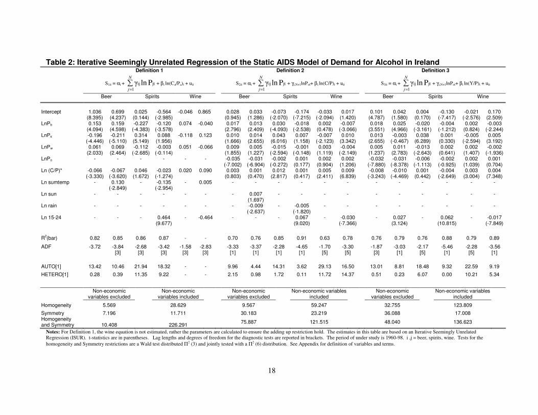
An iterative seemingly unrelated regression (ISUR) procedure is employed to

estimate regressions (10a)-(10c). This procedure adjusts for cross-equation contemporaneous

correlation and consequently takes into account the optimisation process behind the demand

system.7 The results of the parsimonious estimation of these equations are presented in Table

5 The expenditure (at constant prices) in alcohol, as a percentage of personal expenditure has fallen

from 10.5% in 1960 to 8.1% in 1998. In 1960, of the expenditure in alcohol, 75% was on beer, 23% on

spirits and 2% on wine. This breakdown has changed considerably over the last three decades; in 1998,

Irish expenditure on alcohol was divided among beer (65%), spirits (19%) and wine (16%). To

conserve space the data is not presented in this paper but is available from the authors on request. 6 Some of the price and population variables are found to be near I(2) in our sample. However, given

the low power of the ADF test in small samples these variables will be treated as I(1), as they are also a

priori expected to be first difference stationary. To conserve space these are not reported in the paper

but are available by request from the authors. 7 Since SUR is sensitive to the excluded equation (in our case the wine equation), ISUR is used instead

of SUR, as the process of iteration ensures that the obtained estimates asymptotically approach those

of the maximum likelihood method (see Judge, Griffiths, Hill, Lutkepohl and Lee, 1980).

9

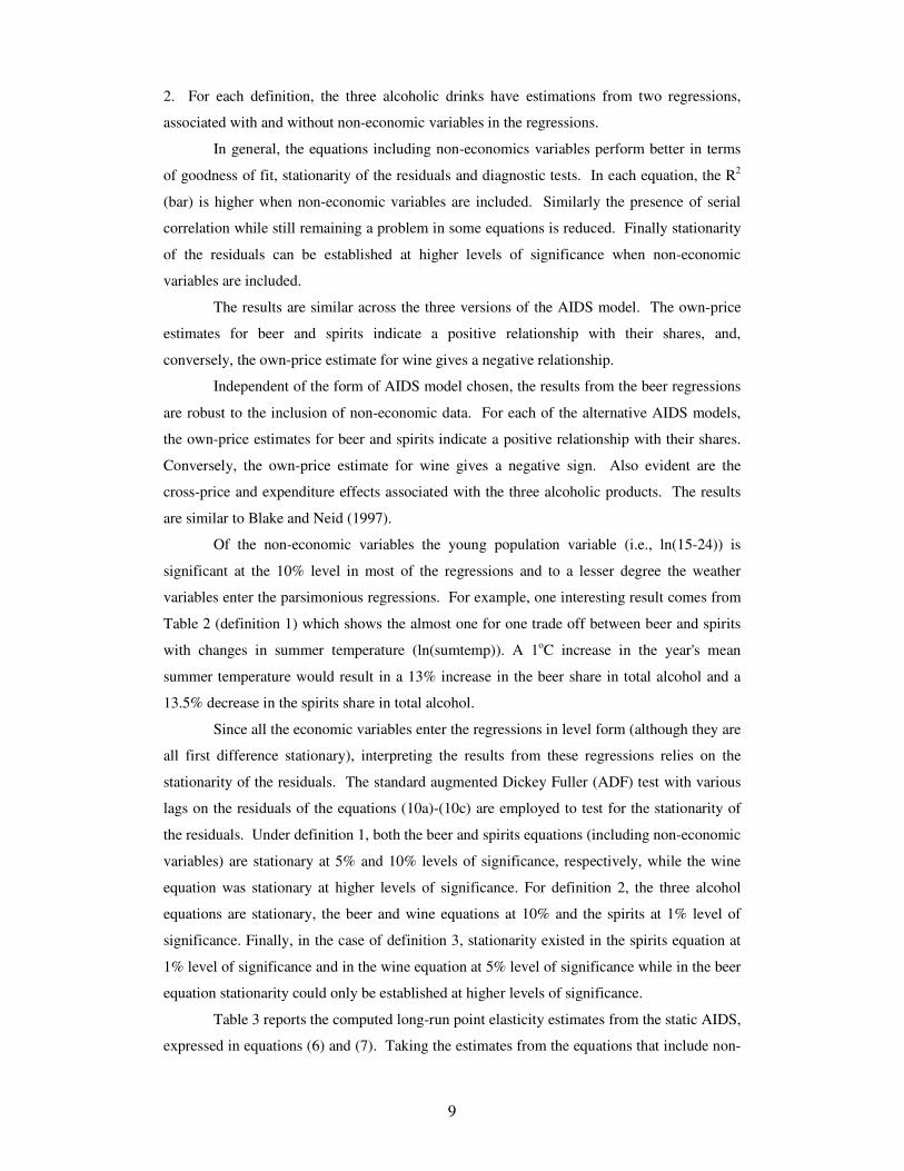
2. For each definition, the three alcoholic drinks have estimations from two regressions,

associated with and without non-economic variables in the regressions.

In general, the equations including non-economics variables perform better in terms

of goodness of fit, stationarity of the residuals and diagnostic tests. In each equation, the R2

(bar) is higher when non-economic variables are included. Similarly the presence of serial

correlation while still remaining a problem in some equations is reduced. Finally stationarity

of the residuals can be established at higher levels of significance when non-economic

variables are included.

The results are similar across the three versions of the AIDS model. The own-price

estimates for beer and spirits indicate a positive relationship with their shares, and,

conversely, the own-price estimate for wine gives a negative relationship.

Independent of the form of AIDS model chosen, the results from the beer regressions

are robust to the inclusion of non-economic data. For each of the alternative AIDS models,

the own-price estimates for beer and spirits indicate a positive relationship with their shares.

Conversely, the own-price estimate for wine gives a negative sign. Also evident are the

cross-price and expenditure effects associated with the three alcoholic products. The results

are similar to Blake and Neid (1997).

Of the non-economic variables the young population variable (i.e., ln(15-24)) is

significant at the 10% level in most of the regressions and to a lesser degree the weather

variables enter the parsimonious regressions. For example, one interesting result comes from

Table 2 (definition 1) which shows the almost one for one trade off between beer and spirits

with changes in summer temperature (ln(sumtemp)). A 1oC increase in the year's mean

summer temperature would result in a 13% increase in the beer share in total alcohol and a

13.5% decrease in the spirits share in total alcohol.

Since all the economic variables enter the regressions in level form (although they are

all first difference stationary), interpreting the results from these regressions relies on the

stationarity of the residuals. The standard augmented Dickey Fuller (ADF) test with various

lags on the residuals of the equations (10a)-(10c) are employed to test for the stationarity of

the residuals. Under definition 1, both the beer and spirits equations (including non-economic

variables) are stationary at 5% and 10% levels of significance, respectively, while the wine

equation was stationary at higher levels of significance. For definition 2, the three alcohol

equations are stationary, the beer and wine equations at 10% and the spirits at 1% level of

significance. Finally, in the case of definition 3, stationarity existed in the spirits equation at

1% level of significance and in the wine equation at 5% level of significance while in the beer

equation stationarity could only be established at higher levels of significance.

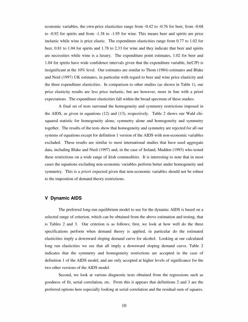
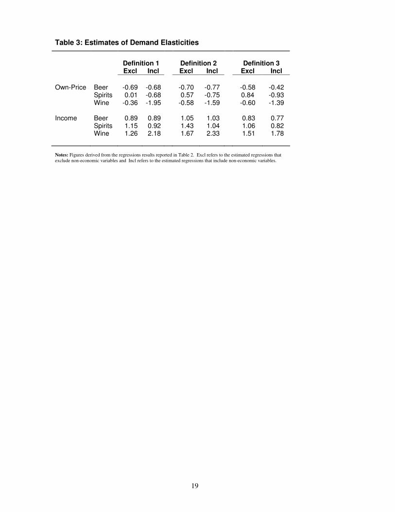
Table 3 reports the computed long-run point elasticity estimates from the static AIDS,

expressed in equations (6) and (7). Taking the estimates from the equations that include non-

10

economic variables, the own-price elasticities range from -0.42 to -0.76 for beer, from -0.68

to -0.92 for spirits and from -1.38 to -1.95 for wine. This means beer and spirits are price

inelastic while wine is price elastic. The expenditure elasticities range from 0.77 to 1.02 for

beer, 0.81 to 1.04 for spirits and 1.78 to 2.33 for wine and they indicate that beer and spirits

are necessities while wine is a luxury. The expenditure point estimates, 1.02 for beer and

1.04 for spirits have wide confidence intervals given that the expenditure variable, ln(C/P) is

insignificant at the 10% level. Our estimates are similar to Thom (1984) estimates and Blake

and Neid (1997) UK estimates, in particular with regard to beer and wine price elasticity and

the three expenditure elasticities. In comparison to other studies (as shown in Table 1), our

price elasticity results are less price inelastic, but are however, more in line with a priori

expectations. The expenditure elasticities fall within the broad spectrum of these studies.

A final set of tests surround the homogeneity and symmetry restrictions imposed in

the AIDS, as given in equations (12) and (13), respectively. Table 2 shows our Wald chi-

squared statistic for homogeneity alone, symmetry alone and homogeneity and symmetry

together. The results of the tests show that homogeneity and symmetry are rejected for all our

systems of equations except for definition 1 version of the AIDS with non-economic variables

excluded. These results are similar to most international studies that have used aggregate

data, including Blake and Nied (1997) and, in the case of Ireland, Madden (1993) who tested

these restrictions on a wide range of Irish commodities. It is interesting to note that in most

cases the equations excluding non-economic variables perform better under homogeneity and

symmetry. This is a priori expected given that non-economic variables should not be robust

to the imposition of demand theory restrictions.

V Dynamic AIDS

The preferred long-run equilibrium model to use for the dynamic AIDS is based on a

selected range of criterion, which can be obtained from the above estimation and testing, that

is Tables 2 and 3. Our criterion is as follows; first, we look at how well do the three

specifications perform when demand theory is applied, in particular do the estimated

elasticities imply a downward sloping demand curve for alcohol. Looking at our calculated

long run elasticities we see that all imply a downward sloping demand curve. Table 2

indicates that the symmetry and homogeneity restrictions are accepted in the case of

definition 1 of the AIDS model, and are only accepted at higher levels of significance for the

two other versions of the AIDS model.

Second, we look at various diagnostic tests obtained from the regressions such as

goodness of fit, serial correlation, etc. From this it appears that definitions 2 and 3 are the

preferred options here especially looking at serial correlation and the residual sum of squares.

11

Third, we consider which model indicates a stationary (long-run) relationship between the

dependent and explanatory variables, i.e. whether the residuals are stationary. The only

version of the AIDS model that satisfies the stationarity condition for the three alcohol

equations is definition 2. Stationarity is only significant at a significance level greater than

10% for the wine equation under definition 1 and for the beer equation under definition 3.

Overall, all three versions of the static AIDS model perform well and give acceptable

results such that any one of the three could be used for estimating a dynamic form. We

choose definition 2 as the preferred model8 mainly because the three alcohol equations are

more strongly stationary which is necessary condition in estimating the dynamic error

correction process. Another important reason for choosing definition 2 over 1 or 3 is that it

uses consumption expenditure data, which is a preferable to disposable income to use in a

demand system like the AIDS.

The disequilibrium of the static AIDS model - definition 2 version - will enable us to

reconcile the short run behaviour of the demand for the individual beverages with their long-

run behaviour. Using (9), the equations that will be estimated are as follows:

(14) ∆S2b,t = α1b+ α2b∆S2b,t-1 + γb0∆lnPb,t + γb1∆lnPb,t-1 + γs0∆lnPs,t + γs1∆lnPs,t-1

+ γw0∆lnPw,t + γw1∆lnPw,t-1 + βb0lnPo,t + βb1lnPo,t-1 + δb0∆ln(C/P)t

+ δb1∆ln(C/P)t-1 + 2b1lnsunt + 2b2lnraint + λbub,t-1 + γt

where ub,t-1 is the estimated residuals lagged one period from the definition 2 version of the

AIDS beer equation

(15) ∆S2s,t = α1s+ α2s∆S2s,t-1 + γb0∆lnPb,t + γb1∆lnPb,t-1 + γs0∆lnPs,t + γs1∆lnPs,t-1

+ γw0∆lnPw,t + γw1∆lnPw,t-1 + βs0∆lnPo,t + βs1∆lnPo,t-1 + δs0∆ln(C/P)t

+ δs1∆ln(C/P)t-1 + 2s1δ1lnraint + 2s2∆ln(15-24)t + 2s3∆ln(15-24)t-1

+ λsus,t-1 + γt

where us,t-1 is the estimated residuals lagged one period from the definition 2 version of the

AIDS spirits equation.

(16) ∆S2w,t = α1w+ α2w∆S2w,t-1 + γb0∆lnPb,t + γb1∆lnPb,t-1 + γs0∆lnPs,t + γs1∆lnPs,t-1

+ γw0∆lnPw,t + γw1∆lnPw,t-1 + βw0∆lnPo,t + βw1∆lnPo,t-1 + δw0∆ln(C/P)t

+ δw1∆ln(C/P)t-1 + 2w1∆ln(15-24)t + 2w2∆ln(15-24)t-1 + λwuw,t-1 + γt

8 We also estimate the dynamic form of the AIDS model under definitions 1 and 3. To conserve space

these are not reported in the paper but are available by request from the authors.

12

where uw,t-1 is the estimated residuals lagged one period from the definition 2 version of the

AIDS wine equation

In the equations above the first-difference terms on the right hand side capture the

short-run disturbances in the respective shares of the individual drinks in total personal

expenditure. We include current values and a lagged value for the changes in prices, changes

in expenditure and changes in population variables to determine whether past or present

values are significant in determining the short run disturbances of the individual drinks. In

estimation, a parsimonious form of equations (14)-(16) is reported.

The error correction term ui where i = beer, spirits and wine, captures the long-run

equilibrium relationship, given by the standard AIDS equation, and λi captures the speed of

adjustment toward the long-run equilibrium. If λi is large or closer to one in absolute value

then there is a rapid adjustment, i.e. the disturbance quickly disappears and we are back along

the long run path. The smaller that λi is the slower the adjustment back to long run

equilibrium. In estimating the dynamic AIDS all variables in equations (14)-(16) must be

stationary. Our climate variables in the beer and spirits equation are entered in level form

since they are I(0), i.e. they are stationary in levels.

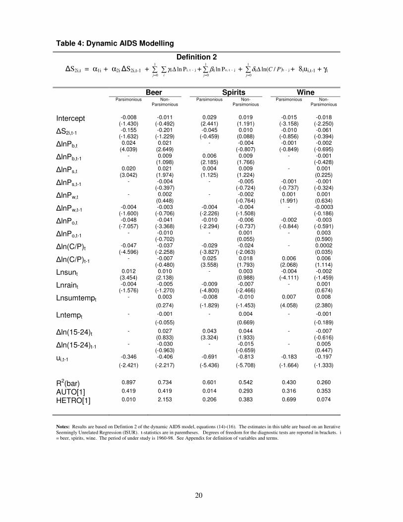
The dynamic AIDS is estimated using an ISUR procedure, and the results for the

system are given in Table 4. Both beer and spirits equations give satisfactory results with

most of the variables significant at 10% levels, the R2 are high and the equations pass all of

the diagnostic tests. Our beer gives a value for λ as -0.4022. This means that 40% of the

disturbance to the long-run equilibrium in the previous period is corrected or adjusted back to

long-run equilibrium in this period. The spirits error correction term (-0.9195) indicates that

consumers are able to adjust spirits consumption to long run equilibrium considerably faster.

90% of the disturbance is corrected or adjusted back to that long-run equilibrium path within

one period. Looking to our wine equation we see that most of the estimates are insignificant

at the 10% level. The R2 is also very low but it still passes all diagnostic tests. The error

correction term (significant at the 12% level) indicates that approximately one-third of the

disturbance to the long-run equilibrium path is corrected within the next period.

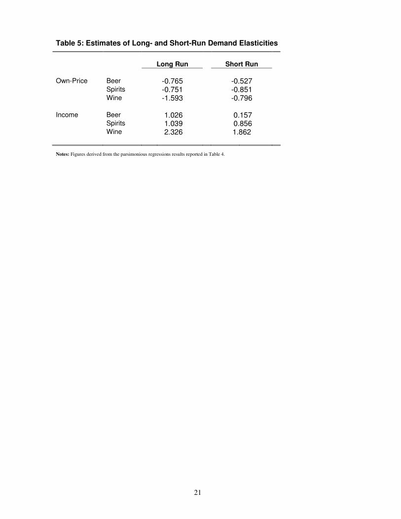
The short run point elasticities were calculated using (6) and (7) and are presented in

Table 7 along with the estimated range for our long run point elasticities. They indicate that

beer is price inelastic while spirits and wine are price elastic. Beer and spirits are found to be

necessities in the short run while wine is a luxury. Using the calculated long-run and short-

run point elasticities and also the calculated error correction term we are now able to interpret

the pattern of demand for the individual drinks.

Looking at the short-run pattern of the demand for beer we estimate a price elasticity

of -0.581. This lies within the range given for the long-run elasticities therefore there exists

13

small changes in the price response between the short and long run. The short-run

expenditure elasticity of 0.144 is minimal and less than that of the long run expenditure

elasticity, hence there is less of a response to expenditure changes in the short run than over

the long run. The short-run own price elasticity for spirits is given as -1.2155, which

indicates that spirits is price elastic in the short run. In the long run, spirits are price inelastic,

this implies a change in demand behaviour for spirits when moving from the short to the long

run. Also given the fact that the speed of adjustment back to the long run equilibrium is very

rapid (as given by λspirits = -0.9195) then the behaviour of spirits demand changes quickly

from being price elastic to being price inelastic, that is, the long-run elasticity9. The

expenditure elasticity lies within the range given by the long run elasticities so again there are

small changes in the expenditure response between the short and long run. Finally wine has

short-run elasticities indicating it to be price elastic and expenditure elastic in the short run, a

result which is of similar magnitude to its long run behaviour. The long-run wine elasticities

are slightly larger in absolute value indicating that responses to changes in price and

expenditure are slightly more sensitive over the long run.

VII Conclusions

This paper uses three versions of Deaton and Muellbauer 's AIDS model to calculate

long-run elasticities of beer, spirits and wine. The demand theory restrictions and other

diagnostic tests all three versions of the static AIDS perform well and the elasticities

calculated (excluding some irrational estimates) are acceptable. From calculating our long-

run elasticities we find that beer and spirits are price inelastic while wine is price elastic. The

own price elasticities range from -0.42 to -0.76 for beer, -0.68 to -0.92 for spirits and -1.38 to

-1.95 for wine. The expenditure elasticities indicate that wine is a luxury (elasticity measure

range from 1.78 to 2.33) while both beer (0.77 to 1.02) and spirits (0.81 to1.04) are

necessities. These point estimates are similar to previous studies (see for example, Thom,

1984, and Blake and Neid, 1997).

In calculating the short-run elasticities we estimated a dynamic error correction form

of the AIDS by employing a one-lagged dynamic data generating process. This was achieved

by selecting one of the three versions of the AIDS model based on selected criteria, which

ranged from demand theory restrictions to the possibility of cointegration between the

dependent and independent variables. Definition 2 of the AIDS, which defines the

expenditure share as that share of expenditure on each alcoholic drink from the total alcohol

expenditure, was taken as the long-run equilibrium model.

9 The coefficient on the spirits price effect is also insignificant, unlike the case for beer. Therefore the

short-run spirits price effect is likely to have wide confidence intervals.

14

We found that in the short run beer was price inelastic while spirits and wine were

price elastic. The expenditure elasticities indicated that beer is a necessity in the short run

while spirits and wine were luxuries. This meant that both beer and wine exhibit the same

behaviour in the short and long run. However the demand for spirits changes from being

price elastic in the short run to be price inelastic in the long run. Moreover using a dynamic

generating process we were able to calculate consumers' speed of adjustment and we found

that consumers are able to adjust spirits consumption to the long-run equilibrium considerably

faster.

Given the significantly high rate of excise duties on alcohol in Ireland, policy

implications of the elasticity measures are relevant. Concentrating on the long run elasticities

we have already seen that both beer and spirits are price inelastic. This suggest that an

increase in price on beer or spirits (due to an increase in excise) will increase tax revenue

since the price change will decrease the quantity demanded ceteris paribus, but not by as

much as the increase in price (tax) and thus increases government revenue. This is all the

more important since excises on beer and spirits provide bigger revenue than excises on wine.

Note however, the ceteris paribus assumption is unlikely to hold in practice. An increase in

tax would increase the incentive for suppliers of alcohol to increase the price they charge to

consumers in order to cover lower profit margins10. The fact that beer and spirits are price

inelastic provides the incentive or opportunity for the government and then also the alcohol

producers to increase price. Therefore the actual excise increase may in fact result in a

reduction in revenue. Hence analysis of consumer demand for alcoholic beverages both in the

long run and in the short run and also analysis that incorporates dynamic industry effects is

necessary in deriving tax/revenue effects on alcohol. This study goes in some way to

supplying such analysis.

The dynamic approach taken in this paper to estimate demand systems has future

applications, among others, in agricultural, health and energy economics. The fact that the

AIDS model is a very popular makes it easier to apply a dynamic AIDS similar to the one

used here.

10 With additional duty on alcohol, profit margins (as a percentage of price) for alcohol would fall.

15

References

Andrikopoulos, A., Brox, J. and Carvalho, E. (1997) "The demand for domestic and imported

alcoholic beverages in Ontario, Canada: a dynamic simultaneous equation approach." Applied

Economics, 29, 945-53.

Blake, D., and Nied A. (1997) "The demand for alcohol in the United Kingdom." Applied

Economics, 29(12), 1655-72.

Buse, A., (1994) "Evaluating the linearised almost ideal demand system." American Journal

of Agricultural Economics, 76, 781-93.

Central Statistics Office. Various Issues. National Income and Expenditure. Government

Stationary Office, Dublin.

Central Statistics Office. Various Issues. Statistical Abstract. Government Stationary Office,

Dublin.

Clements, K.W., and Johnson, L.W. (1983) "The demand for beer, wine and spirits: A

system-wide approach." Journal of Business, 56, 273-304.

Clements, K.W., and Selvanathan E.A. (1987) "Alcohol consumption", in H. Theil and K.W.

Clements (eds), Applied Demand Analysis: Results from System-wide Approaches. Ballinger:

Cambridge, Mass.

Conniffe, D., and McCoy, D. (1993) Alcohol use in Ireland: Some Economic and Social

Implications, General Research Series. Paper No 160. Economic and Social Research

Institute, Dublin.

Deaton, A.S., and Muellbauer J. (1980) "An almost ideal demand system." American

Economic Review, 70, 312-26.

Dickey, D.A., and Fuller, W.A. (1981) "Likelihood ratio statistics for autoregressive time

series with a unit root." Econometrica, 49, 1057-72.

Duffy, M. (1983) "The demand for alcoholic drink in the UK, 1963-78." Applied Economics,

15, 125-40.

Duffy, M. (1987) "Advertising and the inter-product distribution of demand: A Rotterdam

model approach." European Economic Review, 31, 1051-70.

Engle, R.F., and Granger C.W.J. (1987) "Cointegration and error correction: Representation,

estimation and testing." Econometrica, 55, 251-76.

Foley, A. (1999) "Report on the Drinks Industry in Ireland." Commissioned by the Drinks

Industry Group.

Gao X., Wailes, E., and Cramer, G. (1995) "A microeconometric model analysis of US

consumer demand for alcoholic beverages." Applied Economics, 27, 59-69.

Hendry, D.A., Pagan, A.R., and Sargan, J.D. (1984) "Dynamic specification", in Z. Griliches

and M.D. Intriligator (eds), Handbook of Econometrics, Vol. II, Chapter 18. North-Holland:

Amsterdam.

16

Johnson, J., Oksanen, E., Veall, M., and Fretz, D. (1992) "Short-run and long-run elasticities

for Canadian consumption of alcoholic beverages: An error-correction

mechanism/cointegration approach." Review of Economics and Statistics, 74, 64-74.

Jones, A.M. (1989) "A systems approach to the demand for alcohol and tobacco." Bulletin of

Economic Research, 41, 86-101.

Judge, G., Griffiths, W., Hill, R.C., Lutkepohl, H., and Lee, T. (1980) The Theory and

Practice of Econometrics. Wiley: New York.

Karagiannis, G., and Velentzas, K. (1997) "Explaining food consumption patterns in Greece."

Journal of Agricultural Economics, 48, 83-92.

Karagiannis, G., Katranidis S., and Velentzas, K. (2000) "An error correction almost ideal

demand system for meat in Greece." Agricultural Economics, 22, 29-35.

Madden, D. (1993) "A new set of consumer demand estimates for Ireland." Economic and

Social Review, 24(2), 101-23.

McGuinness, T. (1983) "The demand for beer, spirits and wine in the UK,1956-79", in M.

Grant, M. Plant, and A. Williams (eds), Economics and Alcohol. Croom Helm: London.

Nelson J.P., and Moran J.R. (1995) "Advertising and US alcoholic beverage demand: System-

wide estimates." Applied Economics, 27, 1225-36.

Selvanathan, E.A. (1989) "Advertising and alcohol demand in the UK: Further results."

International Journal of Advertising, 8, 181-8.

Selvanathan, E.A. (1991) "Cross-country alcohol consumption comparison: An application of

the Rotterdam demand system." Applied Economics, 23, 1613-22.

Thom, D.R. (1984) "The demand for alcohol in Ireland." Economic and Social Review, 15,

325-36.

Walsh, B., and Walsh D. (1970) "Economic aspects of alcohol consumption in the Republic

of Ireland." Economic and Social Review, 2, 115-38.

17

Table 1: Comparison of Demand Elasticities for Beer, Wine and Spirits

Own price elasticity

Expenditure elasticity

Study Model and period Beer Spirits Wine Beer Spirits Wine

Ireland

Thom (1984) AIDS model -0.59 -1.29 -1.61 0.8 1.386 1.23

1969(1) to 1980(4) to -0.76 to -1.54 to -1.60

Walsh and Linear Model 1953-68 0.09 -0.57 - 0.63 1.94 -

Walsh(1970) to 0.79 to 2.06

Britain

Blake and Neid (1997) AIDS model 1952-91 -0.95 -1.32 -0.95 0.89 0.98 1.61

Clements & Working's Model -0.19 -0.24 -0.23 0.41 1.81 1.91

Selvanathan(1987) 1955-1975

Duffy (1983) Log-Lin, Lin, Simultaneous - 0.8 0.65 0.8 1.6 2.5

Mdls 1963-83 to 1 to 0.87 to 1.1

Duffy (1987) Rotterdam Model 1963-83 -0.29 -0.51 -0.77 0.6 1.42 1.7

Jones (1989) AIDS Model -0.27 -0.95 -0.77 0.31 1.14 1.15

1964-1983 (Quat)

McGuinness (1983) Linear Model 1956-1979 -0.18 -0.3 0.38 0.13 1.54 1.11

Selvanathan (1989) Theil's Differential -0.2 -0.79 -0.49 0.41 2.18 1.74

Approach 1955-1985

Selvanathan (1991) Rotterdam Model 1955-85 -0.13 -0.31 -0.4 0.52 1.83 1.31

United States

Gao et al (1995) AIDS equivalent Model -0.23 -0.40 -0.25 -0.09 5.03 1.21

1987-1989 (cross sectional)

Nelson & Moran (1995) Rotterdam, AIDS(1)

, -0.08 -0.08 -0.26 0.79 1.26 1.06

CBS, NBR 1964-1990

Clements & Working's Model -0.09 -0.1 -0.22 0.75 1.34 0.46

Selvanathan (1987) 1949-1982

Selvanathan (1991) Rotterdam Model -0.11 -0.11 -0.05 0.71 1.36 0.63

1949-1982

Canada

Andrikopoulous AIDS Model -0.48 -0.54 -0.51 0.96 0.083 2.22

et al (1997) 1958-1987

Selvanathan (1991) Rotterdam Model 1953-82 -0.26 -0.01 -0.16 0.71 1.29 0.97

Johnson et al (1992)

Unrestricted ECM

long run elasticity -0.14 0.37 -1.17 0.27 1.02 2.19

to -0.28 to 0.84 to -1.26 to 0.46 to 1.27 to 2.62

short run elasticity -0.3 -0.85 -0.88 0.16 1 1

to -0.45 to -0.70 to 0.48

Australia

Clements & Rotterdam Model -0.11 -0.53 -0.4 0.75 2.32 0.75

Johnson (1983) 1956-1977

Clements & Working's Model -0.12 -0.52 -0.34 0.73 2.5 0.62

Selvanathan (1987) 1956-1977

Selvanathan (1991)

Rotterdam Model 1955-85 -0.15 -0.61 -0.6 0.84 1.94 0.73

Notes: (1) Only the estimates from the AIDS model are reported.

18

Table 2: Iterative Seemingly Unrelated Regression of the Static AIDS Model of Demand for Alcohol in Ireland Definition 1

S1it = αi + ∑=

N

j 1

jtij Plnγ + βi ln(Ca/Pa)t + uit

Definition 2

S2it = αi + ∑=

N

j 1

jtij Plnγ + γi,N+1lnPot+ βi ln(C/P)t + uit

Definition 3

S3it = αi + ∑=

N

j 1

jtij Plnγ + γi,N+1lnPot+ βi ln(Y/P)t + uit

Beer Spirits Wine Beer Spirits Wine Beer Spirits Wine

Intercept 1.036

(8.395) 0.699

(4.237) 0.025

(0.144) -0.564

(-2.985) -0.046

0.865 0.028

(0.945) 0.033

(1.286) -0.073

(-2.070) -0.174

(-7.215) -0.033

(-2.094) 0.017

(1.420) 0.101

(4.787) 0.042

(1.580) 0.004

(0.170) -0.130

(-7.417) -0.021

(-2.576) 0.170

(2.509) LnPb 0.153

(4.094) 0.159

(4.598) -0.227

(-4.383) -0.120

(-3.578) 0.074 -0.040 0.017

(2.796) 0.013

(2.409) 0.030

(-4.093) -0.018

(-2.538) 0.002

(0.478) -0.007

(-3.066) 0.018

(3.551) 0.025

(4.966) -0.020

(-3.161) -0.004

(-1.212) 0.002

(0.824) -0.003

(-2.244) LnPs -0.196

(-4.446) -0.211

(-5.110) 0.314

(5.149) 0.088

(1.956) -0.118 0.123 0.010

(1.666) 0.014

(2.655) 0.043

(6.016) 0.007

(1.158) -0.007

(-2.123) 0.010

(3.342) 0.013

(2.655) -0.003

(-0.467) 0.038

(6.289) 0.001

(0.330) -0.005

(-2.594) 0.005

(3.192) LnPw 0.061

(2.033) 0.069

(2.464) -0.112

(-2.685) -0.003

(-0.114) 0.051 -0.066 0.009

(1.855) 0.005

(1.227) -0.015

(-2.594) -0.001

(-0.148) 0.003

(1.119) -0.004

(-2.149) 0.005

(1.237) 0.011

(2.783) -0.013

(-2.643) 0.002

(0.641) 0.002

(1.407) -0.002

(-1.936) LnPo -

- - - - - -0.035

(-7.002) -0.031

(-6.904) -0.002

(-0.272) 0.001

(0.177) 0.002

(0.904) 0.002

(1.206) -0.032

(-7.880) -0.031

(-8.378) -0.006

(-1.113) -0.002

(-0.925) 0.002

(1.039) 0.001

(0.704) Ln (C/P)* -0.066

(-3.330) -0.067

(-3.620) 0.046

(1.672) -0.023

(-1.274) 0.020 0.090 0.003

(0.803) 0.001

(0.470) 0.012

(2.817) 0.001

(0.417) 0.005

(2.411) 0.009

(6.839) -0.008

(-3.243) -0.010

(-4.469) 0.001

(0.442) -0.004

(-2.649) 0.003

(3.004) 0.004

(7.348) Ln sumtemp - 0.130

(-2.849) - -0.135

(-2.954) - 0.005 - - - - - - - - - - - -

Ln sun - -

- - - - - 0.007 (1.697)

- - - - - - - - - -

Ln rain - -

- - - - - -0.009 (-2.637)

- -0.005 (-1.820)

- - - - - - - -

Ln 15-24 - -

- 0.464 (9.677)

- -0.464 - - - 0.067 (9.020)

- -0.030 (-7.366)

- 0.027 (3.124)

- 0.062 (10.815)

- -0.017 (-7.849)

R2(bar) 0.82 0.85 0.86 0.87 - - 0.70 0.76 0.85 0.91 0.63 0.78 0.76 0.79 0.76 0.88 0.79 0.89

ADF -3.72 -3.84 [3]

-2.68 [3]

-3.42 [3]

-1.58 [3]

-2.83 [3]

-3.33 [1]

-3.37 [1]

-2.28 [1]

-4.65 [1]

-1.70 [5]

-3.30 [5]

-1.87 [3]

-3.03 [1]

-2.17 [5]

-5.46 [1]

-2.28 [5]

-3.56 [1]

AUTO[1] 13.42 10.46 21.94 18.32 - - 9.96 4.44 14.31 3.62 29.13 16.50 13.01 8.81 18.48 9.32 22.59 9.19

HETERO[1] 0.28 0.39 11.35 9.22 - - 2.15 0.98 1.72 0.11 11.72 14.37 0.51 0.23 6.07 0.00 10.21 5.34

Non-economic variables excluded

Non-economic variables included

Non-economic variables excluded

Non-economic variables included

Non-economic variables excluded

Non-economic variables included

Homogeneity 5.569 28.629 9.567 59.247 32.755 123.809

Symmetry 7.196 11.711 30.183 23.219 36.088 17.008 Homogeneity and Symmetry

10.408

226.291 75.887 121.515 48.040 136.623

Notes: For Definition 1, the wine equation is not estimated, rather the parameters are calculated to ensure the adding up restriction hold. The estimates in this table are based on an Iterative Seemingly Unrelated Regression (ISUR). t-statistics are in parentheses. Lag lengths and degrees of freedom for the diagnostic tests are reported in brackets. The period of under study is 1960-98. i ,j = beer, spirits, wine. Tests for the

homogeneity and Symmetry restrictions are a Wald test distributed Π2 (3) and jointly tested with a Π2 (6) distribution. See Appendix for definition of variables and terms.

19

Table 3: Estimates of Demand Elasticities

Definition 1

Definition 2

Definition 3

Excl Incl Excl Incl Excl Incl Own-Price Beer -0.69 -0.68 -0.70 -0.77 -0.58 -0.42 Spirits 0.01 -0.68 0.57 -0.75 0.84 -0.93 Wine -0.36 -1.95 -0.58 -1.59 -0.60 -1.39 Income Beer 0.89 0.89 1.05 1.03 0.83 0.77 Spirits 1.15 0.92 1.43 1.04 1.06 0.82 Wine 1.26 2.18 1.67 2.33 1.51 1.78

Notes: Figures derived from the regressions results reported in Table 2. Excl refers to the estimated regressions that

exclude non-economic variables and Incl refers to the estimated regressions that include non-economic variables.

20

Table 4: Dynamic AIDS Modelling

Definition 2

∆S2i,t = α1i + α2i ∆S2i,t-1 + ∑∑ ∆= ij

j-ti, ij

1

0

Plnγ +∑=

1

0

j-to,ij Plnj

β + ∑=

∆1

0

j-tij )/ln(j

PCδ + 8iui,t-1 + γt

Beer Spirits Wine

Parsimonious Non-Parsimonious

Parsimonious Non-Parsimonious

Parsimonious Non-Parsimonious

Intercept -0.008 (-1.430)

-0.011 (-0.492)

0.029 (2.441)

0.019 (1.191)

-0.015 (-3.158)

-0.018 (-2.250)

∆S2i,t-1 -0.155 (-1.632)

-0.201 (-1.229)

-0.045 (-0.459)

0.010 (0.088)

-0.010 (-0.856)

-0.061 (-0.394)

∆lnPb,t 0.024 (4.039)

0.021 (2.649)

- -0.004 (-0.807)

-0.001 (-0.849)

-0.002 (-0.695)

∆lnPb,t-1 -

0.009 (1.098)

0.006 (2.185)

0.009 (1.766)

- -0.001 (-0.428)

∆lnPs,t 0.020 (3.042)

0.021 (1.974)

0.004 (1.125)

0.009 (1.224)

- 0.001 (0.225)

∆lnPs,t-1 -

-0.004 (-0.397)

- -0.005 (-0.724)

-0.001 (-0.737)

-0.001 (-0.324)

∆lnPw,t -

0.002 (0.448)

- -0.002 (-0.764)

0.001 (1.991)

0.001 (0.634)

∆lnPw,t-1 -0.004 (-1.600)

-0.003 (-0.706)

-0.004 (-2.226)

-0.004 (-1.508)

- -0.0003 (-0.186)

∆lnPo,t -0.048 (-7.057)

-0.041 (-3.368)

-0.010 (-2.294)

-0.006 (-0.737)

-0.002 (-0.844)

-0.003 (-0.591)

∆lnPo,t-1 -

-0.010 (-0.702)

- 0.001 (0.055)

- 0.003 (0.590)

∆ln(C/P)t -0.047 (-4.596)

-0.037 (-2.258)

-0.029 (-3.827)

-0.024 (-2.063)

- 0.0002 (0.035)

∆ln(C/P)t-1 -

-0.007 (-0.480)

0.025 (3.558)

0.018 (1.793)

0.006 (2.068)

0.006 (1.114)

Lnsunt 0.012 (3.454)

0.010 (2.138)

- 0.003 (0.988)

-0.004 (-4.111)

-0.002 (-1.459)

Lnraint -0.004 (-1.576)

-0.005 (-1.270)

-0.009 (-4.800)

-0.007 (-2.466)

- 0.001 (0.674)

Lnsumtempt - 0.003 -0.008 -0.010 0.007 0.008

(0.274) (-1.829) (-1.453) (4.058) (2.380)

Lntempt - -0.001 - 0.004 - -0.001

(-0.055) (0.669) (-0.189)

∆ln(15-24)t -

0.027 (0.833)

0.043 (3.324)

0.044 (1.933)

- -0.007 (-0.616)

∆ln(15-24)t-1 -

-0.030 (-0.963)

- -0.015 (-0.659)

- 0.005 (0.447)

ui,t-1 -0.346 -0.406 -0.691 -0.813 -0.183 -0.197

(-2.421) (-2.217) (-5.436) (-5.708) (-1.664) (-1.333)

R2(bar) 0.897 0.734 0.601 0.542 0.430 0.260

AUTO[1] 0.419 0.419 0.014 0.293 0.316 0.353

HETRO[1] 0.010 2.153 0.206 0.383 0.699 0.074

Notes: Results are based on Defintion 2 of the dynamic AIDS model, equations (14)-(16). The estimates in this table are based on an Iterative

Seemingly Unrelated Regression (ISUR). t-statistics are in parentheses. Degrees of freedom for the diagnostic tests are reported in brackets. i = beer, spirits, wine. The period of under study is 1960-98. See Appendix for definition of variables and terms.

21

Table 5: Estimates of Long- and Short-Run Demand Elasticities

Long Run

Short Run

Own-Price Beer -0.765 -0.527 Spirits -0.751 -0.851 Wine -1.593 -0.796 Income Beer 1.026 0.157 Spirits 1.039 0.856 Wine 2.326 1.862

Notes: Figures derived from the parsimonious regressions results reported in Table 4.

22

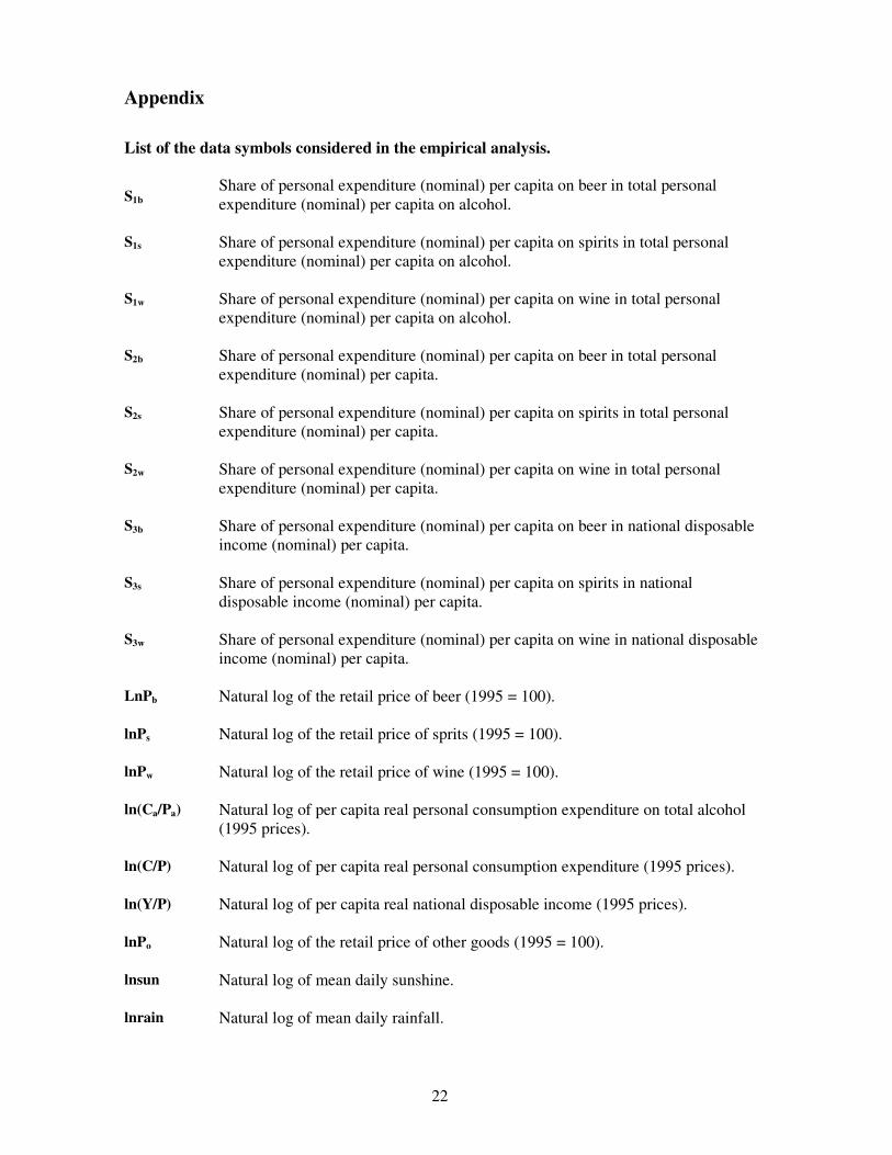
Appendix

List of the data symbols considered in the empirical analysis.

S1b

Share of personal expenditure (nominal) per capita on beer in total personal

expenditure (nominal) per capita on alcohol.

S1s

Share of personal expenditure (nominal) per capita on spirits in total personal

expenditure (nominal) per capita on alcohol.

S1w

Share of personal expenditure (nominal) per capita on wine in total personal

expenditure (nominal) per capita on alcohol.

S2b

Share of personal expenditure (nominal) per capita on beer in total personal

expenditure (nominal) per capita.

S2s

Share of personal expenditure (nominal) per capita on spirits in total personal

expenditure (nominal) per capita.

S2w

Share of personal expenditure (nominal) per capita on wine in total personal

expenditure (nominal) per capita.

S3b

Share of personal expenditure (nominal) per capita on beer in national disposable

income (nominal) per capita.

S3s

Share of personal expenditure (nominal) per capita on spirits in national

disposable income (nominal) per capita.

S3w

Share of personal expenditure (nominal) per capita on wine in national disposable

income (nominal) per capita.

LnPb Natural log of the retail price of beer (1995 = 100).

lnPs Natural log of the retail price of sprits (1995 = 100).

lnPw Natural log of the retail price of wine (1995 = 100).

ln(Ca/Pa) Natural log of per capita real personal consumption expenditure on total alcohol

(1995 prices).

ln(C/P) Natural log of per capita real personal consumption expenditure (1995 prices).

ln(Y/P) Natural log of per capita real national disposable income (1995 prices).

lnPo Natural log of the retail price of other goods (1995 = 100).

lnsun Natural log of mean daily sunshine.

lnrain Natural log of mean daily rainfall.

23

lntemp Natural log of mean daily temperature.

lnsumtemp Natural log of mean daily summer (June, July and August) temperature.

Ln(15-24) Natural log of the percentage of 15-24 year olds in the population over the age of

15.

Definition of the individual alcoholic drinks

Beer Includes stout, ale and lager. Spirits Includes whiskey, gin rum, brandy and other spirits. Wine Includes cider and perry.

Definition of the diagnostic tests

RSS Residual sum of squares.

MEAN Mean of the dependent variable.

AUTO[1] Lagrange multiplier statistic for residual autocorrelation ( χ2 distributed with

1 degree of freedom; 5% critical value = 3.84).

HETERO[1] Langrange multiplier test for heteroscedasticity of the residuals based on a

regression of squared residuals on squared fitted values (χ2 distributed with 1

degree of freedom).

ADF[n] Augmented Dickey-Fuller unit root test statistic on the residuals of the

estimated regression. The ADF is based on

∆xt = α +βx t-1 + γTime + ∑=

n

j 1

δj∆x t-j + vt where xt denotes the residuals of

the regression and [n] denotes lag length to ensure vt is white noise. The

critical values for stationarity of the residuals are (-3.53 at the 5% level and -

3.21 at the 10% level).