Embed Size (px)
Citation preview
User's manual for the groundwater flow model ZOOMQ3D
Groundwater Systems & Water Quality Programme
Internal Report IR/04/140

BRITISH GEOLOGICAL SURVEY
GROUNDWATER SYSTEMS & WATER QUALITY PROGRAMME
INTERNAL REPORT IR/04/140
User's manual for the groundwater flow model ZOOMQ3D
C.R. Jackson and A.E.F. Spink
The National Grid and other Ordnance Survey data are used with the permission of the Controller of Her Majesty’s Stationery Office. Ordnance Survey licence number Licence No:100017897/2004.
Keywords
Groundwater flow model; ZOOMQ3D.
Bibliographical reference
C.R. JACKSON AND A.E.F. SPINK. 2004. User's manual for the groundwater flow model ZOOMQ3D. British Geological Survey Internal Report, IR/04/140. 94pp.
Copyright in materials derived from the British Geological Survey’s work is owned by the Natural Environment Research Council (NERC) and/or the authority that commissioned the work. You may not copy or adapt this publication without first obtaining permission. Contact the BGS Intellectual Property Rights Section, British Geological Survey, Keyworth, e-mail [email protected] You may quote extracts of a reasonable length without prior permission, provided a full acknowledgement is given of the source of the extract.
© NERC 2004. All rights reserved
Keyworth, Nottingham British Geological Survey 2004

The full range of Survey publications is available from the BGS Sales Desks at Nottingham, Edinburgh and London; see contact details below or shop online at www.geologyshop.com
The London Information Office also maintains a reference collection of BGS publications including maps for consultation.
The Survey publishes an annual catalogue of its maps and other publications; this catalogue is available from any of the BGS Sales Desks.
The British Geological Survey carries out the geological survey of Great Britain and Northern Ireland (the latter as an agency service for the government of Northern Ireland), and of the surrounding continental shelf, as well as its basic research projects. It also undertakes programmes of British technical aid in geology in developing countries as arranged by the Department for International Development and other agencies.
The British Geological Survey is a component body of the Natural Environment Research Council.
British Geological Survey offices Keyworth, Nottingham NG12 5GG
0115-936 3241 Fax 0115-936 3488 e-mail: [email protected] www.bgs.ac.uk Shop online at: www.geologyshop.com
Murchison House, West Mains Road, Edinburgh EH9 3LA 0131-667 1000 Fax 0131-668 2683
e-mail: [email protected]
London Information Office at the Natural History Museum (Earth Galleries), Exhibition Road, South Kensington, London SW7 2DE
020-7589 4090 Fax 020-7584 8270 020-7942 5344/45 email: [email protected]
Forde House, Park Five Business Centre, Harrier Way, Sowton, Exeter, Devon EX2 7HU
01392-445271 Fax 01392-445371
Geological Survey of Northern Ireland, 20 College Gardens, Belfast BT9 6BS
028-9066 6595 Fax 028-9066 2835
Maclean Building, Crowmarsh Gifford, Wallingford, Oxfordshire OX10 8BB
01491-838800 Fax 01491-692345
Sophia House, 28 Cathedral Road, Cardiff, CF11 9LJ 029–2066 0147 Fax 029–2066 0159
Parent Body
Natural Environment Research Council, Polaris House, North Star Avenue, Swindon, Wiltshire SN2 1EU
01793-411500 Fax 01793-411501 www.nerc.ac.uk
BRITISH GEOLOGICAL SURVEY

i
Foreword The development of the modelling software within the ZOOM family, of which ZOOMQ3D is a part, has been undertaken through a continuing tripartite collaboration between the University of Birmingham, the Environment Agency and the British Geological Survey. The development of ZETUP and ZOOMQ3D was initially undertaken at the University of Birmingham between 1998 and 2001 but continued after this time as a collaborative project between the three partner organisations. Since the inception of the collaborative project, the development of the software has been directed by the ZOOM steering committee, the members of which are:
University of Birmingham Dr Andrew Spink
Environment Agency Steve Fletcher
Paul Hulme
British Geological Survey Dr Denis Peach
Dr Andrew Hughes
Dr Chris Jackson

ii
Acknowledgements The authors would like to acknowledge the assistance of A.G. Hughes and M.M. Mansour of the British Geological Survey and P.J. Hulme of the Environment Agency for their help in reviewing the ZOOMQ3D software. Additionally, the authors would like to acknowledge the assistance of the following colleagues at the British Geological Survey for reviewing this document: A.G. Hughes and D.G. Kinniburgh.
Preface to the second edition The production of the second edition of the ZOOMQ3D manual coincided with the release of version 1.01 of the groundwater modelling code. This version of the model incorporates some minor adjustments to the original code and some additional functionality. The changes that have been made are described in the following bulleted list. To enable version 1.01 to run models developed using version 1.0, three data files need to be modified. These are (i) the abstraction file (Section 10.2), (ii) the main recharge input file (Section 10.1.3) and (iii) the numeric recharge rate file (Section 10.1.2).
DIFFERENCES BETWEEN VERSION 1.0 AND 1.01 OF ZOOMQ3D
• Multi-layer wells have been added to the code. This enables a pumped borehole to be connected to one or more layers. The pumped well calculates how much water is abstracted from each model layer. The pumped layers do not have to be contiguous. Refer to Section 10.2. The particle tracking code ZOOPT has been updated for use with multi-layer wells.
• All input parameters have been converted to use metres for the unit of length and days for the unit of time. This has required slight modifications to be made to the format of the three input files: (i) the abstraction file (Section 10.2), (ii) the main recharge input file (Section 10.1.3) and (iii) the numeric recharge rate file (Section 10.1.2).
• The rate of leakage between a river node and an aquifer node has been adjusted to better represent river-aquifer interaction under perched conditions. The head that drives leakage into the aquifer is now equivalent to the difference between the river stage and the base of the river bed. Refer to Section 9.5.2.
• All output files containing columns of data have been made space delimited.

iii
Preface to the third edition The production of this third edition of the ZOOMQ3D manual coincides with the release of version 1.03 of the groundwater modelling code. This manual did not need to be updated when version 1.02 was released. Version 1.03 of the model incorporates only some minor adjustments to the code. The changes that have been made are described in the following bulleted list. To enable version 1.03 to run models developed using version 1.02, one data file needs to be modified. This the clock file (Section 10.2).
DIFFERENCES BETWEEN VERSION 1.01 AND 1.03 OF ZOOMQ3D
• A bug has been fixed to correct the calculation of transmissivity in the upper layer of unconfined aquifers. In version 1.01 the transmissivity was limited by the top of the upper layer, which was incorrect. The top of the upper layer is now ignored, if it is unconfined, and the transmissivity is calculated based on the difference between the groundwater head and the base of the layer. The transmissivity was calculated correctly in version 1.01 when the groundwater head was below the top of the upper layer.
• One comment line and one data line have been added to the clock input file to allow the specification of a start time in year month day hh:mm:ss format. This has been implemented because the model has been made OpenMI compliant. See www.openmi.org for more information.
• An additional column has been added to the time-series output files e.g. ‘gauging_stations.out’ (between the third and the fourth column of the output files produced by the previous version of the model). This contains the time in Modified Julian Day format starting from the time specified on the new line in ‘clock.dat’.
• All executables should now be placed in a suitable directory e.g. ‘c:\Program Files\ZOOM’ and this folder should be added to the Windows system PATH variable. The models can then be run from any working directory containing the data files by typing the name of the executable followed by the path of the working directory e.g. ‘ZOOMQ3D c:\myZoomModel’. Alternatively this string can be placed in a batch file and the batch file run from the command line.

iv
Contents Foreword ......................................................................................................................................... i
Acknowledgements........................................................................................................................ ii
Preface to the second edition ........................................................................................................ ii
PART 1 - Discussion...................................................................................................................... 1
1 Introduction ............................................................................................................................ 1
2 Physics of flow ........................................................................................................................ 2
3 The numerical solution process............................................................................................. 5 3.1 Finite difference equations ............................................................................................. 5 3.2 Successive over-relaxation ............................................................................................. 7
4 Capabilities of ZOOMQ3D ................................................................................................. 10 4.1 Features of ZOOMQ3D................................................................................................ 10 4.2 Constructing models using ZETUP.............................................................................. 11 4.3 Terminology ................................................................................................................. 12 4.4 Unit convention ............................................................................................................ 12
5 Running the model ............................................................................................................... 13 5.1 The process of constructing a model ............................................................................ 15
PART 2 – Model input ................................................................................................................ 16
6 Summary of input files required by ZOOMQ3D.............................................................. 16 6.1 The philosophy of model input..................................................................................... 16
7 Model structure .................................................................................................................... 20 7.1 Model structure............................................................................................................. 20 7.2 Confined / unconfined conditions................................................................................. 24 7.3 File formats for inputting spatial data........................................................................... 28 7.4 Representation of layers ............................................................................................... 33 7.5 Hydraulic parameters.................................................................................................... 35
8 Time discretisation and initial conditions .......................................................................... 38 8.1 Time discretisation ....................................................................................................... 38 8.2 Initial groundwater heads ............................................................................................. 42
9 Boundary conditions ............................................................................................................ 44 9.1 Model edge boundary conditions ................................................................................. 44 9.2 Internal fixed heads ...................................................................................................... 44 9.3 Head-dependent leakage nodes .................................................................................... 45 9.4 Springs .......................................................................................................................... 47
v
9.5 Rivers............................................................................................................................ 49
10 Model stresses ....................................................................................................................... 59 10.1 Recharge ....................................................................................................................... 59 10.2 Abstraction and observation wells................................................................................ 65
11 Variable hydraulic conductivity with depth (VKD) ......................................................... 68 11.1 Implementation of VKD in ZOOMQ3D ...................................................................... 69 11.2 VKD input files ............................................................................................................ 72
12 The solution process............................................................................................................. 76 12.1 Successive over-relaxation solution method ................................................................ 76
13 Activating / de-activating nodes.......................................................................................... 78 13.1 De-watering and re-wetting .......................................................................................... 78 13.2 De-activating nodes ...................................................................................................... 80
14 Additional model input files ................................................................................................ 81 14.1 Saving groundwater heads for contouring.................................................................... 81 14.2 Selecting which data input files to use ......................................................................... 82
PART 3 – Model output.............................................................................................................. 83
15 Summary of output files produced by ZOOMQ3D .......................................................... 83 15.1 The philosophy of model ouput.................................................................................... 83 15.2 Processing model output............................................................................................... 83
16 Description of output file formats....................................................................................... 84 16.1 Observation well data ................................................................................................... 84 16.2 Contouring groundwater heads..................................................................................... 84 16.3 Groundwater heads in format to re-start a simulation .................................................. 85 16.4 River flow gauging ....................................................................................................... 85 16.5 River baseflow accretion profiles ................................................................................. 85 16.6 River baseflows in a format to re-start a simulation..................................................... 86 16.7 De-watering and re-wetting .......................................................................................... 88 16.8 Nodal flow balances ..................................................................................................... 88 16.9 Global flow balances .................................................................................................... 89 16.10 Monitoring leakages ..................................................................................................... 90 16.11 Spring flows.................................................................................................................. 91 16.12 Multi-layer wells........................................................................................................... 91 16.13 Convergence of solution............................................................................................... 92 16.14 Variation in transmissivity............................................................................................ 92 16.15 Output files required for particle tracking .................................................................... 92
References .................................................................................................................................... 95

vi
FIGURES
Figure 1 Node numbering in the finite difference stencil .................................................... 5
Figure 2 Starting a command line window from the Windows start menu ....................... 13
Figure 3 Example of changing the working directory within a console window .............. 14
Figure 4 Changing the properties of the console window ................................................. 14
Figure 5 Process of constructing and running a ZOOMQ3D model ................................. 15
Figure 6 Model mesh represented by example ‘grids.dat’ file .......................................... 20
Figure 7 Example ‘grids.dat’ file and format of data ........................................................ 22
Figure 8 Node type parameter values used in ZOOMQ3 defined within ‘grids.dat’ ........ 23
Figure 9 Values of character flag used in ZOOMQ3D to the specify boundary node type defined within ‘grids.dat’ ................................................................................................. 23
Figure 10 Example ‘aquifer.map’ file for defining aquifer conditions in the top model layer .............................................................................................................................. 25
Figure 11 Lines 3 and 4 of input file ‘grids.dat’ for a two layer model .............................. 26
Figure 12 Flow chart of the cyclical transmissivity updating process when simulating unconfined aquifers .......................................................................................................... 27
Figure 13 ‘entry_method.dat’ file format ............................................................................ 29
Figure 14 a) Example mesh composed of four grids and b) representation of the grid hierarchy ........................................................................................................................... 29
Figure 15 Example map file for the entry of spatial data within a layer ............................. 30
Figure 16 Example code file for the entry of spatial data within a layer ............................. 31
Figure 17 Example numeric data file for the entry of spatial data within a layer ............... 32
Figure 18 Calculation of the vertical conductance between layers ..................................... 33
Figure 19 Lines 5 and 6 of input file ‘grids.dat’ .................................................................. 34
Figure 20 Division of time into time-steps, stress periods and blocks ................................ 38
Figure 21 Example ‘clock.dat’ file ...................................................................................... 41
Figure 22 Format of numeric initial groundwater head data file ......................................... 42
Figure 23 Format of ‘leakage.dat’ ....................................................................................... 45
Figure 24 Example ‘leakage.dat’ file ................................................................................... 46
Figure 25 Example ‘springs.dat’ input file .......................................................................... 48
Figure 26 Numbering schemes in ZOOMQ3D for (a) river branches and (b) river nodes for an example model river ............................................................................................... 50
Figure 27 Schematic representation of connections between river and grid nodes ............. 51
Figure 28 Formulation of river-aquifer interaction under influent and effluent conditions . ........................................................................................................................... 53
Figure 29 Specification of flow along or discharge into river at specific river nodes ......... 55
Figure 30 Format of file ‘rivers.dat’ .................................................................................... 56

vii
Figure 31 Format of input file ‘initialflow.dat’ ................................................................... 57
Figure 32 Format of input file ‘river_inputs.dat’ ................................................................. 58
Figure 33 Example code and map file for the entry of recharge data .................................. 59
Figure 34 Example aquifer modelled using two recharge types .......................................... 60
Figure 35 Example model mesh used to simulate aquifer shown in Figure 34 ................... 60
Figure 36 Example recharge time series, recharge code file and recharge map file used to define two different recharge types .................................................................................. 61
Figure 37 Format of numeric recharge data file .................................................................. 62
Figure 38 Example ‘recharge.dat’ file ................................................................................. 64
Figure 39 Conceptualisation of multi-layer well pumping from layers 1, 3 and 5 .............. 66
Figure 40 Example ‘pumping.dat’ file and format of input ................................................. 67
Figure 41 Hypothetical hydraulic conductivity / transmissivity versus depth profile ......... 68
Figure 42 Parameters used to define VKD profiles in ZOOMQ3D .................................... 70
Figure 43 Specification of VKD schemes in ZOOMQ3D ................................................... 71
Figure 44 Example a) VKD scheme map file and b) associated model grid ....................... 73
Figure 45 Example set of a) code and map file and b) numeric data files for VKD parameters on first profile level ........................................................................................ 74
Figure 46 Format of ‘vkd.dat’ input file .............................................................................. 74
Figure 47 Example code file ‘vkdkx01.cod’ and map file ‘vkdkx01.map’ ......................... 75
Figure 48 Example numeric data file ‘vkdkx01.dat’ ........................................................... 75
Figure 49 Format of SOR numerical solver input file ......................................................... 76
Figure 50 Example ‘sor.dat’ file .......................................................................................... 77
Figure 51 Example ‘wetflag##.map’ file ............................................................................. 78
Figure 52 Conceptualisation of wetting threshold at node .................................................. 79
Figure 53 Example ‘nowflow##.map’ file ........................................................................... 80
Figure 54 Example ‘contour_times.dat’ file ........................................................................ 81
Figure 55 Example output file containing river baseflow accretion data ............................ 87
Figure 56 Example global flow balance output file ............................................................. 89
Figure 57 Example ‘transcycle.out’ output file ................................................................... 92
Figure 58 Order of data output to ‘heads.txt’ ...................................................................... 93

viii
TABLES
Table 1 List of all ZOOMQ3D input files ........................................................................... 17
Table 2 ZOOMQ3D input files which are relevant to model features ................................ 18
Table 3 List of minimum set of input files required by ZOOMQ3D when rivers and VKD are not included in the model ........................................................................................... 19
Table 4 Hypothetical recharge rates (mm day-1) for ten stress periods ............................... 59
Table 5 Hypothetical recharge rates (mm day-1) for monthly stress periods ....................... 60
Table 6 Format of ‘zoomq3d.dat’ input file ........................................................................ 82
Table 7 List of all ZOOMQ3D output files ......................................................................... 83
Table 8 Data contained in nodal flow balance output file ................................................... 88
Table 9 Data contained in ‘global_tv.out’ ........................................................................... 90
Table 10 Order of variables listed on line of ‘flowbal.txt’ ................................................. 94
1
PART 1 - Discussion
1 Introduction Numerical groundwater flow models have become an essential tool in the solution of hydrogeological problems. Their importance arises because they are the only real means by which testing of hypotheses can be conducted. It is common to produce what is referred to as a conceptual model, a description of the processes believed to be operating in the groundwater system. However, to assess the validity of the concepts it is essential to produce results from a more physically based model which can be compared with field information. If there is a high degree of similarity between physical model and reality, then the conceptual model can be treated with some confidence. Numerical models provide information based on the physics of the supposed processes and are therefore the best approximation to a physical model.
Fundamental difficulties arise in constructing a numerical model which is going to be able to be close to the real aquifer. Amongst them are recognising the true mechanisms and finding an acceptable numerical implementation. The ability to look at behaviour on different scales is also important. While a relatively coarse approximation, based on a grid spacing of hundreds of metres, may be acceptable for regional flow through a large expanse of relatively homogeneous aquifer, this will not be adequate for small-scale local behaviour. Examples such as the response of an abstraction well or the representation of a small stream will not be dealt with accurately on a coarse mesh.
The process of model development and construction is iterative. Components of the conceptual model are frequently found to be inadequate and require changes. The inability to reproduce features from the real aquifer brings these inadequacies to light. Change and the introduction of new processes are fundamental to the development process.
ZOOMQ3D is a numerical model which advances the art of model development on two vitally important fronts. It incorporates a mesh refinement procedure which aids the solution of problems related to scale. This is the first of its contributions. The second is that it uses object-oriented techniques as the basis for the program. Whilst this is well-established in the development of general commercial software, it represents a novel approach to groundwater model structure. It is of considerable value in maintaining the code but it is in changing model behaviour that it holds most promise for modellers. Further, the direct correspondence between computer-based objects and real-world features makes the link between numerical and conceptual models very easy to see, even to those with no programming expertise.
2
2 Physics of flow ZOOMQ3D is a quasi-three-dimensional groundwater flow model. To understand the implications of its quasi-three-dimensionality, it is convenient to begin with a general three-dimensional groundwater flow equation
Nt
Sz
kzy
kyx
kx szyx −
∂∂
=⎟⎠⎞
⎜⎝⎛
∂∂
∂∂
+⎟⎟⎠
⎞⎜⎜⎝
⎛∂∂
∂∂
+⎟⎠⎞
⎜⎝⎛
∂∂
∂∂ φφφφ
where
( )t,z,y,xφ is the groundwater head value at a point (x,y,z) and at time t [L],
( ) ( ) ( )z,y,xk,z,y,xk,z,y,xk zyx are the hydraulic conductivity values in the x, y and z directions respectively [LT-1],
( )zyxSs ,, is the specific storage at (x, y, z) [L-1],
N(x, y, z, t) is a source flow term as a flow per unit volume [T-1].
This equation is derived by considering a flow balance for an infinitesimally small volume element located anywhere within a body of saturated aquifer. A number of assumptions underlie this equation. First, the fluid is assumed to be of constant density; this allows the flow balance to be a consequence of mass conservation within the element. Next, the Cartesian co-ordinate system is aligned with the principal axes of the hydraulic conductivity tensor; this avoids the need for cross derivatives.
A model, based on the above equation, incorporating appropriate boundary and initial conditions, would be truly three-dimensional. ZOOMQ3D takes a simplifying approach to the solution of the three-dimensional equation by recognising that in many aquifers it is possible to identify a layered structure. If the layers are aligned parallel to the horizontal co-ordinate axes, then the three-dimensional equation can be integrated vertically across the layer to produce an equation which describes the flow within a layer and its interactions with adjacent layers. Such an equation is
belowaboveyx LLqthS
yhT
yxhT
x+−−
∂∂
=⎟⎟⎠
⎞⎜⎜⎝
⎛∂∂
∂∂
+⎟⎠⎞
⎜⎝⎛
∂∂
∂∂
where
( )t,y,xh is the groundwater head value within a layer [L],
( ) ( )yxTyxT yx ,,, are the transmissivity values in the x and y directions respectively [L2T-1],
( )yxS , is the storage coefficient of the layer [L0],
q(x, y, t) is a source flow term as a flow per unit surface area [LT-1],
Labove and Lbelow are leakage rates from layers above and below [LT-1].

3
In layered models, the general approach to obtaining an equation such as the one above is to characterise the flow within a layer by means of a single head value and to use transmissivity as the parameter governing flow within the layer. Storage within a layer is measured by the storage coefficient. Vertical transfers between layers are determined by leakage rates at the upper and lower surfaces.
In mathematical terms, the single groundwater head value is taken to be the average head across the layer. If the groundwater head is ( )tzyx ,,,φ at a general point, the vertically integrated average value is ( )tyxh ,, which is calculated as
( )( )
12
zz
zz
zz
dzt,z,y,xt,y,xh
2
1
−
φ=
∫=
=
where z1 and z2 are the base and top elevations of the layer, respectively.
By a similar process of integrating over the vertical, transmissivity and storage coefficient are evaluated as
( ) ( )∫
=
== 2
1
zz
zz xx dzz,y,xky,xT and ( ) ( )∫=
== 2
1
zz
zz s dzz,y,xSy,xS
and the source term becomes a flow per unit surface area of the aquifer denoted by q(x,y,t).
Unfortunately, the process of integrating the three-dimensional equation does not lead to the quasi-three-dimensional equation and the vertically integrated parameters except in some rather limiting circumstances. In order to demonstrate the limitations, it is necessary to look in detail at the integration of the three-dimensional equation. For the sake of clarity, only the terms involving flow in the x-z plane will be treated here as the behaviour in the y-z plane is similar. The problem then is the evaluation of
∫∫∫∫ −∂φ∂
=⎟⎠⎞
⎜⎝⎛
∂φ∂
∂∂
+⎟⎠⎞
⎜⎝⎛
∂φ∂
∂∂ 2
1
2
1
2
1
2
1
z
z
z
z s
z
z z
z
z x dzNdzt
Sdzz
kz
dzx
kx
Two terms in the equation, the second on the left and right-hand sides, are relatively easy to deal with. The second term on the left-hand side evaluates to
12 zz
zz z
kz
k∂∂
−∂∂ φφ
because it involves only variations in the z-direction. These terms correspond to the leakages in the quasi-three-dimensional equation, Labove and Lbelow, respectively. The second term on the right can be replaced by a source term equal to the net effect of N over the layer thickness expressed as a flow per unit surface area, q, as shown in the quasi-three-dimensional equation.
4
When it comes to dealing with the remaining terms, an important aid in the integration process is the Leibniz Integral Rule which is usually stated in a form used to calculate the differential of a definite integral (Riley et al., 2002, p182)
( )( )
( )
( )
( ) ( )( ) ( )( )xaxa,xf
xbxb,xfdz
xfdzz,xf
xxb
xa
xb
xa ∂∂
−∂∂
+∂∂
=∂∂
∫∫
In the problem examined here, it is in fact the integration of partial derivatives which is important and the rule is re-arranged as follows
( )
( ) ( )( )
( ) ( )( ) ( )( )xaxa,xf
xbxb,xfdzz,xf
xdz
xf xb
xa
xb
xa ∂∂
+∂∂
−∂∂
=∂∂
∫∫
In evaluating the first term on the right-hand side, the function f is replaced by t
Ss ∂∂φ . This
should reduce to thS
∂∂ after integration for consistency with the quasi-three-dimensional
equation. For this to occur, two conditions must be met. The first is that the integration limits are constant; z1 and z2 are independent of x. This implies that the layer boundaries are horizontal. The second is that Ss does not change over the layer thickness. The second limitation is generally unimportant but the first is of considerable significance since layered models are frequently applied to aquifers where the structure is not one of horizontal layering.
The final integral, dealing with the first term on the left-hand side, is also complex. The
function f is replaced by x
kx ∂∂φ . Again, the quasi-three-dimensional result can only be
obtained if the layer boundaries are horizontal. Further, the value of kx must be constant, with the result that the transmissivity is evaluated as kx (z1 – z2) and not the more general integral form. This is a particularly important limitation when a model based on the quasi-three-dimensional equation is used to treat aquifers where hydraulic conductivity varies with depth within a layer.
The previous discussion applies to layers where there is no free surface. The uppermost layer in an unconfined aquifer will contain a free surface and requires further consideration. In a quasi-three-dimensional formulation of a layer open to the atmosphere the usual treatment is to define a transmissivity value calculated based on the current saturated thickness of the upper layer. The groundwater head value which characterises the layer is based on the value at the free surface, not the average within the saturated thickness. Finally, the storage coefficient is set equal to the aquifer specific yield. These features add to the approximations to which the model is subject.
While a quasi-three-dimensional model has numerous theoretical limitations, for many practical problems it represents an acceptable solution. There is a compromise between representing the complexity of real flow systems and the data and computational demands which a three-dimensional model imposes.

5
3 The numerical solution process 3.1 FINITE DIFFERENCE EQUATIONS ZOOMQ3D uses implicit finite difference approximations as the basis for its representation of the layered aquifer flow equation
belowaboveyx LLqthS
yhT
yxhT
x+−−
∂∂
=⎟⎟⎠
⎞⎜⎜⎝
⎛∂∂
∂∂
+⎟⎠⎞
⎜⎝⎛
∂∂
∂∂
To allow the approximation, the aquifer is divided into grid of nodal points at which the groundwater head will be calculated. The calculation proceeds from a known pattern of head values, the initial condition, through a series of discrete time-steps. The nodal groundwater head values at the end of a time-step are all unknown. Each term in the equation has a corresponding finite difference approximation, with those involving flow through the aquifer using groundwater head values at the end of a time-step. By applying the finite difference approximations at each node, a set of simultaneous algebraic equations is formed. The solution to the equations provides the head values at the end of the time-step. The newly calculated values form the known starting values for the next time-step.
To illustrate the structure of the finite difference equations, a typical node will be considered (Figure 1). This node will be referred to as the central node and the groundwater head there will be denoted by hc
* at the beginning of a time-step and hc at the end of the step. In the plane of the layer containing the node, there are usually four surrounding nodes. Two are located at a distance Δx ahead of and behind the central node in the x-direction. These will be referred to as nodes 1 and 3 with groundwater heads h1 and h3, respectively. There are similar nodes, spaced at Δy, in the y-direction denoted as 2 and 4 with groundwater heads h2 and h4.
In the layers above and below that under consideration, nodes are located immediately above the central node. These are referred to as a and b and the corresponding head values are ha and hb. The vertical separation is Δz. Only the head values at the end of the time-step are required for the non-central nodes in an implicit calculation.
Figure 1 Node numbering in the finite difference stencil
c
1 2
3 4
a
b

6
The aquifer flow properties between the nodes form part of the governing equation and the storage and external source terms at each node also arise. The relevant parameters are the x and y-direction transmissivities, Tx and Ty, and the vertical hydraulic conductivities operating between the central node and nodes a and b above and below, ka and kb. These values are derived from nodal hydraulic conductivities in the principal directions, the layer thicknesses and the saturated depth of any unconfined layer which may be present. Details of the relationships are not given here.
The structure of the finite difference approximations in the x and y-directions are similar in form and so only the x-direction term is examined in detail here. The vertical leakage approximations also have a similar structure and only the term relating to flow between the central node and the layer above is quoted.
For flow through the aquifer in the x-direction, the following approximation holds
( ) 23
221
3311 xhT
xhTT
xhT
xhT
x xc
xxxx Δ+
Δ+−
Δ≈⎟
⎠⎞
⎜⎝⎛
∂∂
∂∂
The second suffix on the transmissivity values indicates the appropriate part of the aquifer. For example
1xT is the transmissivity between the central node and node 1.
For vertical leakage between the central and upper node,
( )caa
azzabove hh
zk
zhkL −
Δ≈
∂∂
=
For the rate of change of storage at the node
( )
thhS
thS cc
Δ−
≈∂∂ *
When all the terms are approximated, the resulting equation has the following structure
FhAhAhAhAhAhAhAhA ccccbbaa −−=−−++++ **
44332211
where 211
xT
A x
Δ= , 22
2
yT
A x
Δ= , 23
3
xT
A x
Δ= , 24
4
yT
A x
Δ=
a
za z
kA a
Δ= ,
b
zb z
kA b
Δ= ,
tSAc Δ
=* , qF =
and *4321 cbac AAAAAAAA ++++++=

7
At the beginning of a time-step, values for all the An coefficients can be evaluated from the aquifer properties, the mesh geometry and a knowledge of recharge and abstraction. The unknown head values can be found by forming an equation of the above type at each node and solving the resulting set of equations simultaneously.
At nodes along the interface between areas of mesh refinement, the equations differ slightly from the structure given above. The reason for this is that there are five nodes surrounding the central node in the plane of the layer. There is therefore one extra unknown head and its associated coefficient. The coefficients relating to flow between the nodes in the plane of the layer have a different composition to that illustrated above but the same process of forming a set of equations and solving them simultaneously applies. The technique for solving the equations is outlined in the following section.
3.2 SUCCESSIVE OVER-RELAXATION Algorithms for dealing with simultaneous equations fall into two categories known as direct and iterative methods. In a direct solution the results are obtained by applying a fixed set of operations to the equations; the number and type of operations can be determined before they are carried out. As the name suggests, an iterative method involves the repetition of certain operations until a sufficiently close approximation to the real solution is obtained. A measure of accuracy must be selected and this will determine how many iterations are needed. There is no way of deciding how many iterations will be required a priori. Iterative methods can also be classified as point methods, where the algorithm is applied one node at a time, or as block methods where a group of nodes is treated together. Successive over-relaxation (SOR) is an iterative, point method which is very convenient for dealing with the equations in a model with grid refinement where the number of unknowns varies between nodes.
The basis of all iterative methods is to find a relationship which will change an initial estimate of the solution so that it converges on the required value after a finite number of applications. Successive over-relaxation (SOR) represents the most efficient of a series of related methods which all rely on making use of the basic finite difference equation. In the case of ZOOMQ3D, the structure of the finite difference equation can be expressed as follows
FhAhAhAhAhAhAhA ccbbaanncc ++++++= **
2211 K
where
hc is the unknown groundwater head at the central node,
h1 … hn are the unknown groundwater heads at surrounding nodes on the same layer,
ha and hb are the unknown groundwater heads on layers above and below the central node,
hc* is the known groundwater head at the central node,
Ac, Ac*, A1 …An, Aa and Ab are coefficients,
F is a collection of terms involving known flow rates due to recharge and abstraction,
n is the number of surrounding nodes on the layer containing the central node which will be 4 or 5 depending on presence of mesh refinement.

8
The various coefficients are calculated on the basis of conditions at the start of a time-step. Ac involves transmissivity and mesh spacing values, together with storage and time-step size. The terms A1 to An contain only transmissivity and mesh spacing information while Aa and Ab are related to vertical hydraulic conductivity values and layer thicknesses. Ac
* involves only the storage coefficent and time-step size.
In all members of the family of methods leading to SOR, the format of the iterative formula is similar and is based on the above equation. The first of the series is Jacobi iteration which uses the basic finite difference equation without change. The unknown heads on the right-hand side are treated as known for the duration of a single iteration and the relationship is used to update the central unknown groundwater head hc. An iteration cycle is complete after all the nodes have acted as the central node. At this point a check for convergence to the corrrect solution is conducted and iteration continues until the convergence criterion is satisfied. An important feature of the method is that updated values are not used until the next iteration.
As the mesh is scanned, one updated value is available to be used immediately in progressing to the next node in sequence. This produces an alternative formulation known as Gauss-Seidel iteration which is superior in terms of its rate of convergence. The Jacobi method does converge to the correct solution but it is much slower than Gauss-Seidel iteration. As there is no penalty for using updated values as soon as they are calculated, the Gauss-Seidel method is almost always preferable.
To further develop the iteration formula, the equation representing Gauss-Seidel iteration is written in a more compact form. All the terms with the exception of hc are moved to the right-hand side and incorporated into a single term, R. Then the value for n
ch from the last iteration is added and subtracted, giving
[ ] n
cnc
nc hhRh +−=+1
where the superfixes denote iteration number.
This does not alter the Gauss-Seidel relationship; instead it allows a useful interpretation to be made of the iteration formula. The term in brackets [ ], gives a measure of the change which has been introduced over a single iteration. If this moves the new value closer to the true solution, then it can be argued that a larger change would speed convergence. Within certain limits, this is the case and SOR aims to exploit this fact. A larger change is imposed by increasing the change by a factor ω which is larger than one. If too big a change is imposed then the scheme becomes unstable. An upper limit on ω of 2 avoids this difficulty. It is the fact that a larger change than that defined by Gauss-Seidel is applied which gives the process its name of over-relaxation. When ω is introduced, the relationship is no longer an equality; instead it provides a rule by which new iterations are defined. It is usually expressed in the following form
( ) n
cnc hRh ωω −+=+ 11
The SOR iteration scheme is very easy to incorporate into a computer program and it is generally reliable though not the most rapid technique currently available.

9
3.2.1 Convergence criteria With any iterative scheme there must be some test which is applied to decide that the process has come sufficiently close to the true solution. An apparently attractive option is to test the change in head which arises over an iteration. When this is smaller than a selected value for every node, convergence is assumed. This should not normally be used in groundwater problems because it does not guarantee that the flow balance at a node is satisfied. Flow rates are governed by Darcy's Law and therefore depend on the head gradient. Significant errors can still occur in the gradient even though the head changes are small.
The basic equation represents a flow balance and therefore a test based on satisfying it is much more reliable. This is the approach adopted in ZOOMQ3D. The iterations stop when the basic equation is satisfied to within a specified flow rate. Increased accuracy requires a larger number of iterations and very small errors often require an unacceptable increase in computer time.
Although there are limits imposed on ω, it is necessary to select a value from within the allowed range. This can be very important as the rate of convergence is often sensitive to the choice of ω and it may be worthwhile experimenting with different values, particularly if simulations are long or many options are being explored.
10
4 Capabilities of ZOOMQ3D 4.1 FEATURES OF ZOOMQ3D This section summarises the capabilities of ZOOMQ3D. Each of these features is discussed in detail in the following sections of this manual.
4.1.1 Multiple layers
ZOOMQ3D can incorporate multiple layers of finite difference nodes. The elevation of these layers can vary across the model and the base elevation of one layer can be higher than the top of the layer below it. The separation of model layers simplifies the representation of groundwater systems that contain aquifers separated aquitards. This because the flow through low permeability layers, which is assumed to be vertical, is represented by the vertical leakage term connecting two finite difference nodes within the upper and lower aquifer.
4.1.2 Local grid refinement ZOOMQ3D incorporates a mesh refinement procedure which aids the solution of problems related to scale. The density of finite difference nodes can be increased by adding successively finer rectangular grids in discrete areas of the model domain. The mesh can be refined in separate areas and grids can be refined multiple times in the same location in order to zoom into a specific model feature, for example an abstraction borehole or a river reach.
4.1.3 Confined - unconfined conditions Both confined and unconfined aquifers can be modelled. At confined finite difference nodes transmissivity and storage are independent of groundwater head. At unconfined nodes transmissivity is a function of saturated thickness and the storage term incorporates specific yield. In the top model layer finite different nodes can be defined as being confined, unconfined or convertible. Convertible nodes switch between unconfined and confined behaviour when the groundwater head rises above its top elevation. In each of the lower model layers, all the nodes must be specified as being either confined or convertible.
Finite difference nodes dewater as the groundwater head drops below their base. In this case the node is removed from the matrix of finite difference equations.
4.1.4 Heterogeneity and anisotropy
Models can be heterogeneous and anisotropic. Different hydraulic parameter values can be specified at each finite difference node and hydraulic conductivity may be different in the x and y-directions. It is assumed that the Cartesian co-ordinate system is aligned with the principal axes of the hydraulic conductivity tensor.
4.1.5 Moving boundaries Model nodes can de-water and re-wet. Nodes are made inactive when the groundwater level falls below their base and vice versa. The re-wetting of model nodes depends on the groundwater head in adjacent finite difference nodes.
4.1.6 Variable hydraulic conductivity with depth (VKD) Vertical variations in hydraulic conductivity with depth can be specified within model layers or across model layers by defining VKD profiles. The transmissivity at a node is calculated by integrating the hydraulic conductivity over the vertical saturated thickness of the node.

11
4.1.7 Recharge Recharge can vary spatially and temporally. Recharge is always applied to the upper-most active node.
4.1.8 Abstraction wells
Pumped boreholes can be placed at any node within the model domain. Abstraction rates can vary temporally and wells can both abstract water from the aquifer and inject water into it.
4.1.9 Rivers Dendritic rivers basins are simulated using a series of interconnected river reaches. The hydraulic parameters characterising a reach can vary along the river as can the degree of connection with the aquifer. The transfer of water between the aquifer and rivers is simulated as is the accretion of baseflow along each river branch. Discharges to the river can be specified in any reach, for example to represent a sewage treatment works, and the discharge rate can vary over time. Both fully penterating and perched rivers can be simulated.
4.1.10 Head-dependent leakage nodes
In addition to rivers, a second head-dependent leakage mechanism is included in ZOOMQ3D. The flow through leakage nodes is proportional to the difference between its elevation and the groundwater head at the finite difference node to which it is connected. Flow can occur in either direction i.e. into or out of the aquifer. Leakage nodes can be used to model spring flows, lakes or estuaries, for example.
4.1.11 Springs This model feature has been developed to simulated spring flows specifically. The flow out of a spring depends on the transmissivity of the surrounding finite difference nodes. Spring flows are represented by an ‘abstraction’ which removes water from the aquifer at the location of the spring until the water table falls below the level of the ground surface.
4.1.12 Time discretisation Simulation time is divided into time-steps, stress periods and blocks. The length of a time-step is equivalent to the length of time between which successive solutions are calculated for the model’s state variables. A stress period represents a period of time during which all model stresses remain constant e.g. recharge, groundwater abstraction or discharge to rivers. Stress periods are divided into one or more time-steps. A block is composed of one or more stress periods. The rationale for the use of blocks is predominantly related to the simplification of the organisation of time-variant data, for example, groundwater abstraction or recharge rates, within input files. The number of stress periods in each block is the same for all blocks within a simulation.
4.2 CONSTRUCTING MODELS USING ZETUP ZETUP is the pre-processor for the finite difference groundwater flow model ZOOMQ3D (Jackson and Spink, 2004). It is used to construct the model grid, which may contain multiple areas of local grid refinement, and to create rivers within these complex meshes. ZETUP produces the input files required by ZOOMQ3D that define the structure of the model mesh and the structure of rivers. It also produces generic templates of all of the other files required by ZOOMQ3D in the correct format. These can be modified subsequently using a text editor to complete the model specification. Finally, ZETUP produces a set of files that enable the

12
visualisation and checking of the model structure. If modifications to the structure of the model are required, it can be reloaded into ZETUP for alteration.
4.3 TERMINOLOGY ZOOMQ3D is written using an object-oriented programming language. Whilst the users do not need to concern themselves with what this means, the term object is used a number of times within this manual and consequently, a brief explanation is required.
The user can think of an object in abstract terms as any distinct entity that stores data and perform tasks. In ZETUP and ZOOMQ3D objects are defined to represent real world features. For example, a pumped well is represented by an object. Pumped wells are described by data such as a depth and radius, and have the capability to pump water out of an aquifer. References are made in this manual to objects, which represent finite difference grids and rivers.
4.4 UNIT CONVENTION All lengths in ZOOMQ3D must be specified in metres. The unit of time is specified as days. All volumetric flow rates are input and output in m3day-1.

13
5 Running the model To install ZOOMQ3D on a Windows PC copy the executable ‘zoomq3d.exe’ into suitable directory such as ‘c:\Program Files\ZOOM’. Then add this directory to the Windows system PATH variable (Control Panel System Advanced Tab Environment Variables). No installation procedure is run in which ZOOMQ3D program files are added to the system registry. All the input files required by ZOOMQ3D must be located in a single directory. All the output files produced by ZOOMQ3D will be created in the same directory. It is strongly recommended that ZETUP and ZOOMQ3D are never run using the same working directory and that their files are kept within separate folders.
ZOOMQ3D should be run from the command line in a console window and not started from Windows Explorer. In the event that an error occurs, messages are written to the screen. If ZOOMQ3D is run from Explorer it may terminate before the user is able to read error messages. To start a command window select ‘Run’ from the Windows start menu and type ‘cmd’ in the drop down list box (Figure 2). The user should then change directory to that of the working directory where the ZOOMQ3D input files are located. For help on the commands used to change directory type ‘help cd’ within the console window (Figure 3). To run the model type ‘zoomq3d’ followed by the path to the working directory on the command line e.g. ‘zoomq3d c:\myZOOMQ3D_project’. Alternatively, this string can be placed in a batch file (a text file with a .bat extension e.g. ‘runzoom.bat’) and the name of this batch file can be typed on the command line (omit the extension when doing this e.g. type ‘runzoom’).
Figure 2 Starting a command line window from the Windows start menu

14
Figure 3 Example of changing the working directory within a console window
The size of the console box can be adjusted by clicking on the icon in the top left hand corner of its window and selecting ‘Properties’ from the menu list. Suitable values for the width and height of the window and its associated screen buffer are shown in Figure 3.
Figure 4 Changing the properties of the console window

15
5.1 THE PROCESS OF CONSTRUCTING A MODEL To construct a model and run ZOOMQ3D the process shown in Figure 5 is performed. This involves running the pre-processor ZETUP to construct i) the ZOOMQ3D model input files defining the model structure and ii) the remaining set of generic template input files, for modification using a text editor, to complete the specification of the model. All the input files are then transferred to the directory where the ‘zoomq3d.exe’ executable file is located before ZOOMQ3D is run.
Figure 5 Process of constructing and running a ZOOMQ3D model
START
Run ZETUP to create: 1. Set of ZOOMQ3D input files
defining model structure.
2. Set of remaining ZOOMQ3D input files. These are generic templates and require modification to complete the specification of the model.
Transfer files to ZOOMQ3D
working directory
Run ZOOMQ3D

16
PART 2 – Model input
6 Summary of input files required by ZOOMQ3D 6.1 THE PHILOSOPHY OF MODEL INPUT The philosophy behind the structure of ZOOMQ3D model input is to separate different types of data between files. That is, each file contains one specific type of information only. Whilst this results in the model requiring many input files compared to other models, they all have a very simple format and are easily modified using a text editor. For example, one file contains all information relating to pumping rates, another to observation wells, and another river gauging stations. Generic templates of all of these files are generated by ZETUP. These are in the correct format but the data contained within some requires modification in order to complete the model specification. The following points should be recalled when modifying ZOOMQ3D input files:
1. Values are read into the model in ‘free format’ and consequently, the user does not need to ensure that the number of decimal places and field width are correct for each input value contained in each file.
2. The correct number of parameters must be entered on the correct line of an input file.
3. Whilst it does not matter whether the user enters a decimal number as an integer, it is not permissible to enter an integer as a decimal number.
4. Some but not all files contain comment lines. These are actually text data strings, which are read by the model and discarded.
5. The maximum length of a comment line is 128 characters.
6. It is good practice but not necessary to remove white space from the end of lines.
7. Comments cannot be appended to the end of lines of data. If these are included the model will crash.
8. Comments can be appended to the ends of files.
9. The names of all files are fixed except those defined in the input file ‘zoomq3d.dat’.
10. For some data sets, one file is required per model layer. In this case the layer number is appended (as a two digit integer number) to the end of the file name before the file extension. For example hydcond01.dat, hydcond02.dat etc when defining hydraulic conductivity distributions.
The list of input files required by ZOOMQ3D is presented in Tables 1, 2 and 3. In Table 1 the files are listed in alphabetical order, whereas in Table 2 they are grouped into categories. Though there are thirty-nine files listed, not all of these are required for all simulations. For example, if no rivers are included the model, only one of the files is required from the group of four that relate to rivers. Table 3 lists the minimum set of data files required to run ZOOMQ3D when rivers and VKD are not included in the model. Each of the ZOOMQ3D input files is described in the following section.

17
Table 1 List of all ZOOMQ3D input files
Input file name Relevant section
1 anisotropy##.map & anisotropy##.cod OR anisotropy##.dat per layer 7.5.2 2 aquifer.map 7.2.1 3 boundary.dat 9.1 4 clock.dat 8 5 contour_times.dat 14.1 6 entry_method.dat 7.3.1 7 fixedheads.dat 9.2 8 gauging_stations.dat 9.5.5 9 grids.dat 7.1 10 hydcond##.map & hydcond##.cod OR hydcond##.dat per layer 7.5.1 11 initialflow.dat 9.5.3 12 initialh##.map & initialh##.cod per layer 8.2 13 initialh.dat 8.2 14 leakage.dat 9.3 15 noflow##.map per layer 13.2 16 obsleak.dat 9.3.1 17 obswells.dat 10.2.2 18 pumping.dat 10.2.1 19 recharge.dat 10.1.3 20 recharge.cod & recharge.map & / OR recharge_rates.dat 10.1 21 rivers.dat 9.5.2 22 river_inputs.dat 9.5.4 23 sor.dat 12.1 24 specstor##.map & specstor##.cod specstor##.dat per layer 7.5.3 25 springs.dat 9.4 26 syield##.map & syield##.cod syield##.dat per layer 7.5.4 27 vcond##.map & vcond##.cod OR vcond##.dat per layer 7.4 & 7.5.528 vkd.cod & vkd.map 11.2.1 29 vkd.dat 11.2.2 30 vkdkx##.map & vkdkx##.cod OR vkdkx##.dat per vkd scheme 11.2.2 31 vkdky##.map & vkdky##.cod OR vkdky##.dat per vkd scheme 11.2.2 32 vkdzp##.map & vkdzp##.cod OR vkdzp##.dat per vkd scheme 11.2.2 33 vkdgrad##.map & vkdgrad##.cod OR vkdgrad##.dat per vkd scheme 11.2.2 34 wetflag##.map per layer 13.1.1 35 wethead##.map & wethead##.cod wethead##.dat 13.1.3 36 wetthresh##.map & wetthresh##.cod wetthresh##.dat 13.1.2 37 zbase##.map & zbase##.cod OR zbase##.dat per layer 7.4.2 38 zoomq3d.dat 14.2 39 ztop##.map & ztop##.cod OR ztop##.dat per layer 7.4.1
Note the names of these files are fixed. The names of the remaining files can be specified by the user in the input file ‘zoomq3d.dat’

18
Table 2 ZOOMQ3D input files which are relevant to model features
Model feature Relevant file names Relevant section
Grid structure grids.dat 7.1
Confined / unconfined conditions aquifer.map grids.dat
7.2.1 7.1
Layer elevations 1. Layer top elevations 2. Layer base elevations
ztop##.map & ztop##.cod, or ztop##.dat grids.dat zbase##.map & zbase##.cod, or zbase##.dat
7.4.1 7.1
7.4.2
Entry of spatial data entry_method.dat 7.3.1
Hydraulic parameters 1. Hydraulic conductivity 2. Anisotropy 3. Specific storage 4. Specific yield 5. Vertical conductance
hydcond##.map & hydcond##.cod, or hydcond##.dat anisotropy##.map & anisotropy##.cod, or anisotropy##.dat specstor##.map & specstor##.cod, or specstor##.dat syield##.map & syield##.cod, or syield##.dat vcond##.map & vcond##.cod, or vcond##.dat
7.5.1 7.5.2 7.5.3 7.5.4
7.4 & 7.5.5
Initial groundwater heads initialh##.map & initialh##.cod, or initialh.dat 8.2
Boundary conditions 1. Model edge boundary
conditions 2. Internal fixed heads 3. No flow 4. Head-dependent leakage
nodes 5. Springs
boundary.dat fixedheads.dat noflow##.map leakage.dat, obsleak.dat springs.dat
9.1
9.2
13.2 9.3
9.4
Rivers rivers.dat, initialflow.dat, gauging_stations.dat, river_inputs.dat
9.5
Recharge recharge.dat, recharge.map, recharge.cod, recharge_rates.dat 10.1
Wells 1. Abstraction wells 2. Observation wells
pumping.dat obswells.dat
10.2.1 10.2.2
De-watering and re-wetting wetflag##.map wetthresh##.map & wetthresh##.cod, or wetthresh##.dat wethead##.map & wethead##.cod, or wethead##.dat
13.1.1 13.1.2 13.1.3
Variable hydraulic conductivity with depth (VKD)
vkd.cod & vkd.map vkd.dat vkdkx##.map & vkdkx##.cod, or vkdkx##.dat vkdky##.map & vkdky##.cod, or vkdky##.dat vkdzp##.map & vkdzp##.cod, or vkdzp##.dat vkdgrad##.map & vkdgrad##.cod, or vkdgrad##.dat
11.2.1 11.2.2 11.2.2 11.2.2 11.2.2 11.2.2
Time discretisation clock.dat 8
Numerical solver sor.dat 12.1
Producing head contours contour_times.dat 14.1
Controlling data input zoomq3d.dat 14.2

19
Table 3 List of minimum set of input files required by ZOOMQ3D when rivers and VKD are not included in the model
Input file name Relevant section
1 anisotropy##.map & anisotropy##.cod OR anisotropy##.dat per layer 7.5.2 2 aquifer.map 7.2.1 3 boundary.dat 9.1 4 clock.dat 8 5 contour_times.dat 14.1 6 entry_method.dat 7.3.1 7 fixedheads.dat 9.2 8 grids.dat 7.1 9 hydcond##.map & hydcond##.cod OR hydcond##.dat per layer 7.5.1 10 initialh##.map & initialh##.cod per layer 8.2 11 initialh.dat 8.2 12 leakage.dat 9.3 13 noflow##.map per layer 13.2 14 obsleak.dat 9.3.1 15 obswells.dat 10.2.2 16 pumping.dat 10.2.1 17 recharge.dat 10.1.3 18 recharge.cod & recharge.map & / OR recharge_rates.dat 10.1 19 rivers.dat 9.5.2 20 sor.dat 12.1 21 specstor##.map & specstor##.cod specstor##.dat per layer 7.5.3 22 springs.dat 9.4 23 syield##.map & syield##.cod syield##.dat per layer 7.5.4 24 vcond##.map & vcond##.cod OR vcond##.dat per layer 7.4 & 7.5.525 vkd.cod 11.2.1 26 wetflag##.map per layer 13.1.1 27 wethead##.map & wethead##.cod wethead##.dat 13.1.3 28 wetthresh##.map & wetthresh##.cod wetthresh##.dat 13.1.2 29 zbase##.map & zbase##.cod OR zbase##.dat per layer 7.4.2 30 zoomq3d.dat 14.2 31 ztop##.map & ztop##.cod OR ztop##.dat per layer 7.4.1
Note the names of these files are fixed. The names of the remaining files can be specified by the user in the input file ‘zoomq3d.dat’

20
7 Model structure 7.1 MODEL STRUCTURE The file describing the structure of the model is created by ZETUP and is called ‘grids.out’. For input to ZOOMQ3D it must be renamed ‘grids.dat’. The file contains nodal information for each point in each grid. Blocks of grid data are listed in grid level order beginning with the base grid. An example of ‘grids.dat’ is listed in Figure 7. This relates to the model mesh shown in Figure 6, which consists of a coarse base grid, two subgrids on the first level of refinement and a third refined grid, at the finest scale, on the second level of grid refinement. The format of this input file is described in the second column of Figure 7.
The data on lines 1 to 6 of ‘grids.dat’ can be adjusted by the user, however, the remainder of the file should not be modified. This data is generated by ZETUP and defines the structure of the model mesh. If the user wishes to modify the mesh, the model should be uploaded into ZETUP and altered using this tool.
700 m
700
m
Figure 6 Model mesh represented by example ‘grids.dat’ file
7.1.1 Lines 1 to 6 of ‘grids.dat’
The first three pairs of lines in the input file ‘grids.dat’ contain a comment line and a data line. The parameter specified in the first of these three pairs of lines is the number of layers in the model. This can be modified manually but this would then require the user to check the existence and structure of other ZOOMQ3D input files. If the number of layers is increased, additional input files must be produced, because one file must be created for each layer for some file types. Furthermore, the structure of the file, ‘boundary.dat’, would have to be altered.
The parameters specified in the second of these three pairs of lines are used to specify the type of aquifer conditions operating within each model layer. Each layer can be specified as
21
confined (c) or convertible (v) depending on the conceptual model of the aquifer. This feature is described in detail in Section 7.2.
The parameter specified in the third of these three pairs of lines is used to specify whether the bottom elevations of model layers can be different from the top elevations of the layers beneath them. If an ‘n’ is entered in the input file, the top elevations are read for the top model layer only. The top elevations of each lower layer are made equal to the bottom elevation of the layer above it. If a ‘y’ is entered, data files are read for both the bottom and top elevation of each model layer. The facility to specify a gap between two numerical layers is implemented when, for example, a low permeability layer exists between two aquifers. This feature is described in more detail in Section 7.2.1.
7.1.2 Line 7 onwards of ‘grids.dat’ After the first six lines in ‘grids.dat’, data is specified defining the structure of the model mesh. This data is generated by ZETUP and should not be adjusted by the user. If the user wishes to modify the mesh structure, the model should be uploaded into ZETUP and modified using this tool. However, it is worthwhile understanding the structure of this data.
The seventh and eight line of the input file are also a comment line and a data line. The information specified here defines the number of grid levels in the model and the number of grids on each level. There is only ever one grid on the first level as this is the base grid.
In the ‘grids.dat’ file shown in Figure 7 four blocks of grid data are defined, which relate to the four grids shown in Figure 6. The first relates to the base grid. The second and third blocks correspond to the grids on level two and the fourth block relates to the finest grid on grid level three. Data describing the base grid is slightly different from that describing the subgrids. Following the three lines at the start of each grid block, information about each node is defined. Nodes are listed in row and column sequential order from the bottom to the top of each grid. Information associated with a node located on rows or columns of two or more grids is defined within the highest grid level block. For example, the second subgrid on level two consists of four mesh intervals in both the x and y directions. Consequently, it contains 52 or 25 nodes. However, the data file indicates that there are only 16 blocks of node data defined for this grid. The reason for this is that nine of the nodes also exist in the base grid.
The first line in a block of node data is a comment line composed of a series of dashes. This is used to separate data for each node. On the second line of a block of node data, a variable indicating node type is defined. These variable are integers and take one of five values: 7, 11, 13, 14 or 15. The node types, corresponding to each integer flag are shown in Figure 8. The first four values indicate nodes on the boundary of a refined grid. Nodes of type 15, or 0xf in hexadecimal, are conventional nodes based on a five-point finite difference stencil.
Data on the third line of a node block relates to the position of the node with respect to the boundary. If the first parameter is a ‘b’ the node is located on the model boundary. Otherwise it is inside the model domain and represented by an ‘i’. The second parameter is the boundary node type shown in Figure 9. The third parameter is the relative area of the node. For nodes inside the model boundary this is always 1.0, however, this value can be either 0.25, 0.5 or 0.75 if it is located on the boundary (see Figure 9).

22
Line ‘grids.dat’ Format of data
User
adjusted
BASE GRID – LEVEL 1
SUBGRID – LEVEL 2
SUBGRID – LEVEL 2
SUBGRID – LEVEL 3
1 2 3 4 5 6 7 8 9 10 11 12 13 14 15 16 17 18 19 20 21 22 23 24 25 26 27 28 29 30 31 32 33 34 35 36 37 38 39 40 41 42 43 44 45 46 47 48 49 50 51 52 53 54
----- Number of layers ----- 2 ----- Layer types: confined(c) or convertible(v). From top to bottom ----- v c ----- Read layer top elevations (y/n) ----- n ========== GRID DATA ============= 3 1 2 1 ---------------------------------- 1 2 64 1 1 7 7 0 0 700 700 ------------------- 1 1 0 0 15 b d 0.25 ------------------- 2 1 100 0 15 b k 0.5 ------------------- etc for nodes on base grid ---------------------------------- 2 1 72 8 8 100 100 300 300 4 4 ------------------- 2 1 125 100 13 i u 1 ------------------- 3 1 150 100 13 i u 1 ------------------- etc for nodes on this refined grid ---------------------------------- 2 0 16 4 4 400 400 600 600 2 2 ------------------- 2 1 450 400 13 i u 1 ------------------- 4 1 550 400 13 i u 1 ------------------- etc for nodes on this refined grid ---------------------------------- 3 0 56 8 8 150 150 250 250 2 2 ------------------- 2 1 162.5 150 13 i u 1 ------------------- 4 1 187.5 150 13 i u 1 ------------------- etc for nodes on this refined grid
---- Comment line Number of model layers ---- Comment line Layer type for each layer from top to bottom of model ---- Comment line Character variable specifying if reading layer top elevations ---- Comment line Number of grid levels followed by number of grids on each level ---- Comment line: start of grid data block separator Grid level, number of subgrids, number of nodes in grid, (i,j) of start point on boundary Number intervals in x & y directions, co-ords of SW & NE corners of grid ---- Comment line: node block separator i, j, x and y co-ords of node, node type Boundary node flag, boundary node type, nodal area factor ----- Comment line and two data lines for each node in the grid. Blank lines do not exist ---- Comment line: start of grid data block separator Grid level, number of subgrids, number of nodes in grid No. intervals in x & y directions, co-ords of SW & NE corners, no. x & y parent divisions ---- Comment line: node block separator i, j, x and y co-ords of node, node type Boundary node flag, boundary node type, nodal area factor ----- Comment line and two data lines for each node in the grid. Blank lines do not exist ---- Comment line: start of grid data block separator Grid level, number of subgrids, number of nodes in grid No. intervals in x & y directions, co-ords of SW & NE corners, no. x & y parent divisions ---- Comment line: node block separator i, j, x and y co-ords of node, node type Boundary node flag, boundary node type, nodal area factor ----- Comment line and two data lines for each node in the grid. Blank lines do not exist ---- Comment line: start of grid data block separator Grid level, number of subgrids, number of nodes in grid No. intervals in x & y directions, co-ords of SW & NE corners, no. x & y parent divisions ---- Comment line: node block separator i, j, x and y co-ords of node, node type Boundary node flag, boundary node type, nodal area factor ----- Comment line and two data lines for each node in the grid. Blank lines do not exist
Figure 7 Example ‘grids.dat’ file and format of data

23
Direction N E S W N E S W N E S W N E S W N E S W
Binary node type 1 1 0 1 1 1 1 0 0 1 1 1 1 0 1 1 1 1 1 1
Decimal node type 13 14 7 11 15
Hex node type 0xd 0xe 0x7 0xb 0xf
Nodal location
Figure 8 Node type parameter values used in ZOOMQ3 defined within ‘grids.dat’
Figure 9 Values of character flag used in ZOOMQ3D to the specify boundary node type defined within ‘grids.dat’
A B
D C
E F
G H
I
J
K
L
Relativeareas of 0.25
Relativeareas of 0.75
Relativeareas of 0.5

24
7.2 CONFINED / UNCONFINED CONDITIONS Both confined and unconfined conditions can be simulated within each layer of the model. This is achieved by specifying whether each node in the upper model layer is confined, convertible or unconfined and, whether each lower layer is composed of confined or convertible nodes. The definitions of these three terms is as follows.
Confined nodes
At a confined node the transmissivity and storage are fixed and independent of groundwater head. Transmissivity is calculated using the expression
( )BT zzKT −⋅=
0T = for Bzh ≤
and the storage is defined as
( )BTs zzSS −⋅=
0S = for Bzh ≤
where T is the transmissivity in the x or y-direction, K is the horizontal hydraulic conductivity in the x or y-direction, S is the storage coefficient [L0], Ss is the specific storage [L-1], Tz is the elevation of the top of the node,
Bz is the elevation of the base of the node.
Convertible nodes
The transmissivity and storage of a convertible node is equivalent to that of a confined node if the groundwater head is above the top of the node. However, the transmissivity and confined storage coefficient depend on the groundwater head when it falls below the top of the node. Convertible nodes then calculate transmissivity and elastic storage based on the difference between the groundwater head and the elevation of their base. These are linear relationships as the horizontal hydraulic conductivity and specific storage are assumed to be uniform in the vertical direction. When the groundwater head falls below the top of a convertible node, releases of storage from the free surface i.e. specific yield, contribute to the total storage. The expressions used to calculate transmissivity are
( )BT zzKT −⋅= for Tzh ≥
( )BzhKT −⋅= for Tzh <
0T = for Bzh ≤
The expressions used to calculate total storage are
( )BTs zzSS −⋅= for Tzh ≥
( ) yBs SzhSS +−⋅= for Tzh <
0S = for Bzh ≤
where yS is the specific yield

25
Unconfined nodes At unconfined nodes transmissivity and elastic storage depend on groundwater head. The storage term also contains the component of specific yield. The top elevation of the node is ignored and consequently, there is no upper limit on the transmissivity or confined storage.
The expressions used to calculate transmissivity are
( )BzhKT −⋅= for Bzh >
0T = for Bzh ≤
The expressions used to calculate total storage are
( ) yBs SzhSS +−⋅= for Bzh >
0S = for Bzh ≤
7.2.1 Defining the spatial distribution of confined / unconfined conditions Different types of aquifer nodes can be defined within different areas of the top model layer (layer 01). The file ‘aquifer.map’ is used to specify whether nodes are confined, convertible or unconfined in layer 01. This map file contains a single array, or multiple arrays if grid refinement is incorporated, which is/are composed of the characters ‘c’, ‘v’ or ‘u’. The letters relate to confined, convertible or unconfined conditions, respectively.
These character arrays are listed in grid level order and are separated by a comment line. The comment lines contain information required to identify to which grid each array relates. ZETUP, the set up program for ZOOMQ3D, produces this file and writes the co-ordinates of the bottom left and top right hand corners of the mesh within the comment lines. Consequently, the user need only adjust the letters in the arrays in order to modify the representation of the aquifer. An example of a simple map file is presented in Figure 10. This shows an aquifer, which is unconfined towards the left hand boundary and confined along the right hand edge of the model. A number of convertible nodes are used to represent the transition from unconfined to confined conditions, for example where the aquifer dips below a confining unit. Map files are described in detail in the next section and consequently, only a simple example of the file format is presented here.
---- Map for grid on level: 1 Bottom left: 0,0 Top right: 10000,10000 ---- uuuuvvvcccc uuuuvvvcccc uuuuvvvcccc uuuuvvvcccc uuuuvvvcccc uuuuvvvcccc uuuuvvvcccc uuuuvvvcccc uuuuvvvcccc uuuuvvvcccc uuuuvvvcccc
Figure 10 Example ‘aquifer.map’ file for defining aquifer conditions in the top model layer

26
The type of aquifer conditions operating in the lower layers is defined on line 4 of the input file ‘grids.dat’. Each layer (including the top layer) is defined as either confined (c) or convertible (v) on this line. The character relating to the top layer is read but ignored as this information is specified in more detail in the input file ‘aquifer.map’. All nodes in lower layers are defined as either of confined type or convertible type. Nodes can only be of the unconfined type if they are located within the top model layer.
----- Layer types: confined(c) or convertible(v). From top to bottom ----- v c
Figure 11 Lines 3 and 4 of input file ‘grids.dat’ for a two layer model
7.2.2 Simulating unconfined conditions: updating transmissivity Some groundwater models update transmissivity at the end of each iteration of a numerical solver during the solution of a time-step. This method is not adopted in ZOOMQ3D because it means that the system of finite difference equations is modified whilst their solution is sought. Instead in ZOOMQ3D the transmissivity at convertible and unconfined nodes is recalculated at the end of a time-step, the solution of which can be repeated.
Unconfined behaviour is modelled within a cyclical process. The finite difference equations can be solved once or repeatedly during each time-step. Each unconfined node calculates its transmissivity at the beginning of the time-step based on the groundwater head. A solution to the finite difference equations is then computed. The transmissivity is subsequently recalculated using the newly calculated heads. An average is then taken of the pre and post-solution transmissivities at each convertible and unconfined node. A new solution to the finite difference equations is computed again using these average transmissivity values. This cyclical process continues until the change in transmissivity over a cycle falls below a maximum value or until a maximum number of cycles have been performed.
The test for convergence within the repetitive cycle is based on a maximum permissible change in transmissivity. At the end of a cycle, after the solution has been computed the change in transmissivity is examined at each node. If the maximum change in transmissivity is below a user defined value the solution then progresses to the next time-step. This process is illustrated in Figure 12.
The maximum permissible change in transmissivity and the maximum number of cycles are defined by the user on the second line of the input file relating to the solver, for example ‘sor.dat’ (see Section 12). If the user specifies only one cycle then the solution for each time-step will be calculated only once, with transmissivity being recalculated at its start.
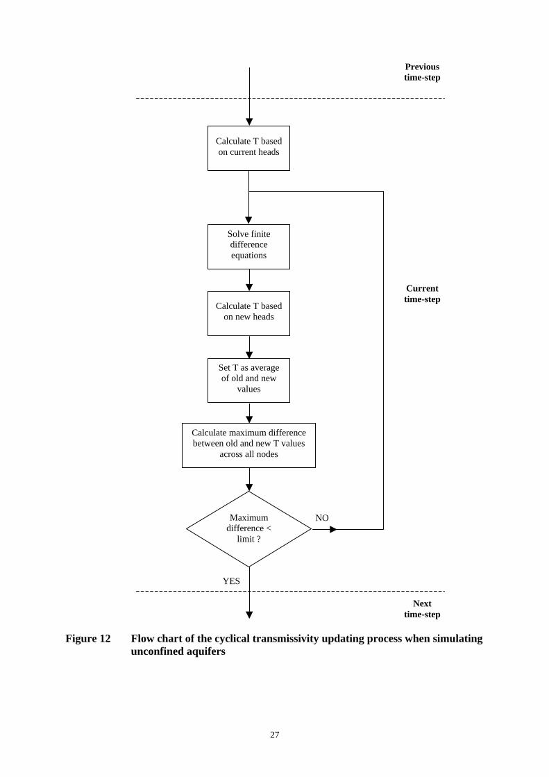
27
Figure 12 Flow chart of the cyclical transmissivity updating process when simulating unconfined aquifers
Calculate T based on current heads
Solve finite difference equations
Calculate T based on new heads
Calculate maximum difference between old and new T values
across all nodes
Maximum difference <
limit ?
Previous time-step
Next time-step
YES
NO
Current time-step
Set T as average of old and new
values
28
7.3 FILE FORMATS FOR INPUTTING SPATIAL DATA Spatial information can be entered into the model using two different methods, or sets of input files. These methods employ either
1. map and code input files or,
2. numeric input data files
In method 1 a pair of ASCII text files is required for each model layer with the file extensions map and cod. A map file contains a single array, or multiple arrays if grid refinement is incorporated, of characters in the range [ a, b, ... y, z, A, B, ...Y, Z ] to define zones of different parameter values. That is, the range is composed of the lower case alphabet followed by the upper case alphabet. Each array represents one of the grids contained in the model. These characters define zones across the model mesh at which a particular value of a parameter is specified. The values of the parameters are specified in the corresponding file with the cod extension. A maximum of fifty-two zones can be used to define the spatial distribution of model parameters when using this method. The name of each of these pairs of files is suffixed with a two-digit number that represents the model layer that the data applies to. For example, the pair of files ‘hydcond01.map’ and ‘hydcond01.cod’ would be used to specify the spatial distribution of hydraulic conductivity in layer 01, the upper model layer.
In method 2 a single ASCII text file is required for each model layer with the dat file extension. Each of these files contains a single array, or multiple arrays, of numeric data with each array representing one of the grids contained in the model. These numbers specify the value of a specific parameter at each finite difference node within the model directly. The name of each of these files is suffixed with a two-digit number that represents the model layer that the data applies to. For example, the file ‘hydcond03.dat’ would be used to specify the spatial distribution of hydraulic conductivity in layer 03, i.e. two layers below the top layer of finite difference nodes.
7.3.1 Selection of spatial data entry method Either of the methods described above can be used to assign values for each of the parameters that can vary spatially across the model domain. To specify which data entry method is to be used, the user must adjust the input file ‘entry_method.dat’. The format of this file is shown in Figure 13. It consists of a series of integers, each of which is preceded by a comment line. There is also an additional comment line at the top of the file. Each comment line, except for the first, notifies the user of the related parameter, e.g. specific yield. The entry mode of the specified parameter is entered on the next line as an integer value. If this integer is equal to 1, a pair of map and code files is required for each model layer. If the integer is equal to 2, one numeric data file, with the dat extension, is required for each layer.

29
// Entry method 1: Map and codes files 2: Raw data // Base elevations 2 // Top elevations 2 // Specific storage 1 // Specific yield 2 // Hydraulic conductivity 2 // Anisotropy 1 // VKD 1 // Vertical conductance 2 // Wetting thresholds 1 // Post wetting heads 1 // Porosity 1
Figure 13 ‘entry_method.dat’ file format
7.3.2 Specifying spatial data using map and code files In this method the spatial distribution of parameter values is defined using ‘maps’. These maps are contained in files with the map extension. For example ‘hydcond02.map’ would be used to define hydraulic conductivity in layer 02 of the model, i.e. one layer down from the top layer. The map files contain one character array for each grid in the model. For example, in Figure 14 the model mesh is composed of four grids: the coarsest base grid, two child grids (on grid level 2) and one grandchild grid (on grid level 3). Consequently, four character arrays are required in each of the map files for this example model. These are listed in grid level order and are separated by a comment line.
Grid level 1Base grid8 columns by 8 rows
Grid level 25 columns by 5 rows
Grid level 29 x 9
Gridlevel 39 x 9
a) b) Figure 14 a) Example mesh composed of four grids and b) representation of the grid
hierarchy

30
The structure of the map file for this example model is shown in Figure 15. As described above, this contains four character arrays separated by comment lines. The comment lines contain information required to identify to which grid each array relates. ZETUP, the set up program for ZOOMQ3D, produces this file and writes the co-ordinates of the bottom left and top right hand corners of the mesh within the comment lines. Consequently the user need only adjust the letters in the arrays in order to modify the model’s parameter values.
---- Map for grid on level: 1 Bottom left: 0,0 Top right: 700,700 ---- aaaaaaaa bbbbbbbb cccccccc dddddddd eeeeeeee ffffffff gggggggg hhhhhhhh ---- Map for grid on level: 2 Bottom left: 100,100 Top right: 300,300 ---- bbbbbbbbb bbbbbbbbb bbbbbbbbb bbbbbbbbb bbbbbbbbb aaaaaaaaa aaaaaaaaa aaaaaaaaa aaaaaaaaa ---- Map for grid on level: 2 Bottom left: 400,400 Top right: 600,600 ---- abcde abcde abcde abcde abcde ---- Map for grid on level: 3 Bottom left: 150,150 Top right: 250,250 ---- aaaaaaaaa aaaaaaaaa aaaaaaaaa aaaaaaaaa aaaaaaaaa aaaaaaaaa aaaaaaaaa aaaaaaaaa aaaaaaaaa
Figure 15 Example map file for the entry of spatial data within a layer
Each letter in the array represents a value of a parameter that is specified in the corresponding code file i.e. the file with the same name but with the cod extension. Code files have the same structure as map files, except each of the character arrays is replaced by a set of data defining the values of the letters contained within the array.
The code file which corresponds to this example model and map file is shown in Figure 16. Similarly to the map file, the code file contains four sets of data separated by comment lines. The comment lines contain the information required to identify to which grid each data set relates. Again, ZETUP, the set up program for ZOOMQ3D, produces this file and writes the co-ordinates of the bottom left and top right hand corners of the mesh within the comment lines. Consequently, the user need only adjust the parameter values for each grid.
In Figure 15, eight letters are used in the base grid, so eight parameter values must be defined in the code file for this grid. On the second grid listed in the map file, only two zones are defined (by the letters ‘a’ and ‘b’) and consequently only two parameter values must be assigned in the code file for this grid. This relationship is the same for the final two grids in

31
the map file. Re-iterating, because eight letters are defined on the base grid in the map file, eight corresponding parameter values must be defined in the code file for this grid. The first integer number in each block of data between the comment lines in the code file is the number of zones, or letters, specified in the character array. After this integer value, an equivalent number of parameter values must be specified. Therefore, for example if twenty-six letters were used in the map file for a specific grid, i.e. the letters a to z, twenty-six parameters values must defined within the code file for the corresponding grid.
In the above description it is stated that there must be an equivalent number of parameter values specified in the code file to the number of letters used in the corresponding character array in the map file. However, this is not strictly the case. In fact, there must be at least the same numbers of parameters specified in the code file as are used in the map file for the corresponding grid. Therefore it is allowable for example, to specify, parameter values for all fifty-two characters in the range [ a, b, ... y, z, A, B, ...Y, Z ] but only use a subset of these letters in the map file.
The final rule to follow when editing the map and code files is that, the minimum number of parameters to enter in the code file is determined by the ‘highest’ letter in the range [ a, b, ... y, z, A, B, ...Y, Z ]. For example, if C is the ‘highest’ letter used then twenty-nine parameters values must be defined in the code file. Similarly, if m is the ‘highest’ letter used then thirteen parameters values are required. This means that if only the two letters ‘a’ and ‘z’ are used to define a grid character array in a map file, at least twenty-six parameters values must still be defined in the corresponding code file for the corresponding grid. This is because the parameter values defined in code files must be listed in the order ‘a’ to ‘z’ then ‘A’ to ‘Z’ i.e. in alphabetical order with the lower case alphabet preceding the upper case alphabet in the fifty-two character scheme.
---- Codes for grid on level: 1 Bottom left: 0,0 Top right: 700,700 ---- 8 1.0 1.2 1.4 2.0 0.1 0.2 0.3 0.7 ---- Codes for grid on level: 2 Bottom left: 100,100 Top right: 300,300 ---- 2 1.0 2.0 ---- Codes for grid on level: 2 Bottom left: 400,400 Top right: 600,600 ---- 5 1.3 1.5 0.9 0.8 0.7 ---- Codes for grid on level: 3 Bottom left: 150,150 Top right: 250,250 ---- 1 0.5
Figure 16 Example code file for the entry of spatial data within a layer

32
7.3.3 Specifying spatial data using numeric data files Instead of using a pair of map and code files to specify the spatial variation of a parameter within a model layer, a single data file can be used containing raw numeric data. This has the same name as the map and code files but has the dat extension. For example, the file ‘specstor04.dat’ could be used to specify specific storage values in layer 04 of the model (i.e. three layers down from the top layer) instead of the files ‘specstor04.map’ and ‘specstor04.cod’. The numeric data file has the same structure as the map file except that each character array is replaced by an array of numbers representing the parameter values that will be applied at the corresponding nodes of the finite difference mesh within the model layer that the file relates to.
An example numeric data file is shown in Figure 17. This specifies exactly the same model data as that specified in the example above, in which a pair of map and code files are used for defining a hydraulic conductivity distribution.
---- Map for grid on level: 1 Bottom left: 0,0 Top right: 700,700 ---- 1.0 1.0 1.0 1.0 1.0 1.0 1.0 1.0 1.2 1.2 1.2 1.2 1.2 1.2 1.2 1.2 1.4 1.4 1.4 1.4 1.4 1.4 1.4 1.4 2.0 2.0 2.0 2.0 2.0 2.0 2.0 2.0 0.1 0.1 0.1 0.1 0.1 0.1 0.1 0.1 0.2 0.2 0.2 0.2 0.2 0.2 0.2 0.2 0.3 0.3 0.3 0.3 0.3 0.3 0.3 0.3 0.7 0.7 0.7 0.7 0.7 0.7 0.7 0.7 ---- Map for grid on level: 2 Bottom left: 100,100 Top right: 300,300 ---- 2.0 2.0 2.0 2.0 2.0 2.0 2.0 2.0 2.0 2.0 2.0 2.0 2.0 2.0 2.0 2.0 2.0 2.0 2.0 2.0 2.0 2.0 2.0 2.0 2.0 2.0 2.0 2.0 2.0 2.0 2.0 2.0 2.0 2.0 2.0 2.0 2.0 2.0 2.0 2.0 2.0 2.0 2.0 2.0 2.0 1.0 1.0 1.0 1.0 1.0 1.0 1.0 1.0 1.0 1.0 1.0 1.0 1.0 1.0 1.0 1.0 1.0 1.0 1.0 1.0 1.0 1.0 1.0 1.0 1.0 1.0 1.0 1.0 1.0 1.0 1.0 1.0 1.0 1.0 1.0 1.0 ---- Map for grid on level: 2 Bottom left: 400,400 Top right: 600,600 ---- 1.3 1.5 0.9 0.8 0.7 1.3 1.5 0.9 0.8 0.7 1.3 1.5 0.9 0.8 0.7 1.3 1.5 0.9 0.8 0.7 1.3 1.5 0.9 0.8 0.7 ---- Map for grid on level: 3 Bottom left: 150,150 Top right: 250,250 ---- 0.5 0.5 0.5 0.5 0.5 0.5 0.5 0.5 0.5 0.5 0.5 0.5 0.5 0.5 0.5 0.5 0.5 0.5 0.5 0.5 0.5 0.5 0.5 0.5 0.5 0.5 0.5 0.5 0.5 0.5 0.5 0.5 0.5 0.5 0.5 0.5 0.5 0.5 0.5 0.5 0.5 0.5 0.5 0.5 0.5 0.5 0.5 0.5 0.5 0.5 0.5 0.5 0.5 0.5 0.5 0.5 0.5 0.5 0.5 0.5 0.5 0.5 0.5 0.5 0.5 0.5 0.5 0.5 0.5 0.5 0.5 0.5 0.5 0.5 0.5 0.5 0.5 0.5 0.5 0.5 0.5
Figure 17 Example numeric data file for the entry of spatial data within a layer
7.3.4 Definition of data at coincident points on multiple grids
It is apparent from the example model and input files described above that parameters values at particular finite difference nodes are specified more than once in an input file when the model mesh is locally refined. This occurs at those nodes on a refined grid that are coincident with the nodes on a coarser grid. Where this occurs the data defined on the refined grid will always override that defined on the coarse mesh.

33
7.4 REPRESENTATION OF LAYERS Vertical discretisation of the model grid is incorporated through the inclusion of layers of finite difference nodes, which are continuous across the model domain. The vertical discretisation is implemented by specifying the number of layers and the conductance between them. Because the vertical conductance term embodies the layer thickness they are not explicitly included in the finite difference equations. However, the elevations of the layers are required by other model mechanisms, for example, the de-watering and re-wetting of model nodes. Such mechanisms require that the top and bottom elevations of the layers be defined explicitly.
The equations used to calculate the vertical conductance between two nodes are presented in Figure 18, which also shows the two different representations of hydrogeological layers possible within the model. The first illustrates the case where two nodes either fall within a single hydrogeological unit or are located at the midpoints of two vertically adjacent hydrogeological units. The second case illustrates the inclusion of a semi-permeable hydrogeological layer in the model without its explicit representation by a layer of finite difference nodes. The input files used to specify vertical conductance within the model are described in Section 7.5.5.
Figure 18 Calculation of the vertical conductance between layers
1ZΔ
2ZΔ2ZK
1ZK
2Z
2
1Z
1
K2/Z
K2/Z
1cetanConduc
VerticalΔ
+Δ
=
a)
Z′Δ
2ZΔ2ZK
ZK′
2Z
2
Z1Z
1
K2/Z
KZ
K2/Z
1cetanConduc
VerticalΔ
+′′Δ
+Δ
=
b)
1ZK1ZΔ

34
7.4.1 Layer bottom elevations The elevation of the bottom of each node within each layer must be specified using either,
1. pairs of map and code files with the names ‘zbase##.map’ and ‘zbase##.cod’ or,
2. numeric data files with the names ‘zbase##.dat’.
The ## symbols must be replaced by a two digit (01 to 99) number representing the layer to which the data files refer. The upper layer is layer 01 and their numbers are incremented from the top to the bottom of the model. Either a pair of map and code files is required for each of the model layers or a single numeric data file is required for each of the layers. The format of these files is described in Section 7.3. The user specifies whether map and code files or numeric data files are used in the input file ‘entry_method.dat’.
7.4.2 Layer top elevations Layer top elevations must be explicitly defined for either the top layer only or for all model layers. The user selects which of these options applies by adjusting the character flag on line 6 of the input file ‘grids.dat’. The section of this input file containing this flag is shown in Figure 19.
----- Read layer top elevations (y/n) ----- n
Figure 19 Lines 5 and 6 of input file ‘grids.dat’
The character variable on line 6 of ‘grids.dat’ is used to specify whether the bottom elevations of model layers can be different from the top elevations of the layers beneath them. If an ‘n’ is defined, the top elevations are read for the top model layer only (layer 01). In this case only the pair of input files, ‘ztop01.map’ and ‘ztop01.cod’ or only the single input file ‘ztop01.dat’ needs to be created. The top elevations of each lower layer are then made equal to the bottom elevation of the layer above it.
If a ‘y’ is entered on line 6 of ‘grids.dat’, data files containing the layer top elevations are required for each of the model layers. In this case the elevation of the top of each node within each layer must be specified using either,
1. pairs of map and code files with the names ‘ztop##.map’ and ‘ztop##.cod’ or,
2. numeric data files with the names ‘ztop##.dat’.
The ## symbols must be replaced by a two digit (01 to 99) number representing the layer to which the data files refer. The upper layer is layer 01 and their numbers are incremented from the top to the bottom of the model. Either a pair of map and code files is required for each of the model layers or a single numeric data file is required for each of the layers. The format of these files is described in Section 7.3. The user specifies whether map and code files or numeric data files are used in the input file ‘entry_method.dat’.

35
7.5 HYDRAULIC PARAMETERS The spatial distribution of a number of hydraulic parameters must be defined within the model. Input files must be prepared for each of the parameters for each layer in the model. The format of these input files is described in Section 7.3.
7.5.1 Hydraulic conductivity (Kx) Only hydraulic conductivity values in the x-direction are read directly by the model. Hydraulic conductivity in the y-direction is calculated as the product of the hydraulic conductivity in the x-direction and an anisotropy ratio.
Input file names and format Hydraulic conductivity in the x-direction must be entered into the model using either,
1. pairs of map and code files with the names ‘hydcond##.map’ and ‘hydcond##.cod’ or,
2. numeric data files with the names ‘hydcond##.dat’.
The ## symbols must be replaced by a two digit (01 to 99) number representing the layer to which the data files refer. The upper layer is layer 01 and their numbers are incremented from the top to the bottom of the model. Either a pair of map and code files is required for each of the model layers or a single numeric data file is required for each of the layers. The format of these files is described in Section 7.3. The user specifies whether map and code files or numeric data files are used in the input file ‘entry_method.dat’.
7.5.2 Anisotropy Hydraulic conductivity in the y-direction is calculated by the model as the product of the hydraulic conductivity in the x-direction and the anisotropy ratio, xy KK . All values greater than or equal to zero are valid as input.
Input file names and format
Anisotropy ratio data must be entered into the model using either,
1. pairs of map and code files with the names ‘anisotropy##.map’ and ‘anisotropy##.cod’ or,
2. numeric data files with the names ‘anisotropy##.dat’.
The ## symbols must be replaced by a two digit (01 to 99) number representing the layer to which the data files refer. The upper layer is layer 01 and their numbers are incremented from the top to the bottom of the model. Either a pair of map and code files is required for each of the model layers or a single numeric data file is required for each of the layers. The format of these files is described in Section 7.3. The user specifies whether map and code files or numeric data files are used in the input file ‘entry_method.dat’.
7.5.3 Specific storage Input files containing specific storage data must defined for each model layer. Specific storage has units of m-1. The confined storage coefficient of each finite difference node is calculated by multiplying the specific storage by a vertical saturated thickness. The thickness used depends on whether the node is of the confined, convertible or unconfined type. The following expressions hold for each of the nodal types.
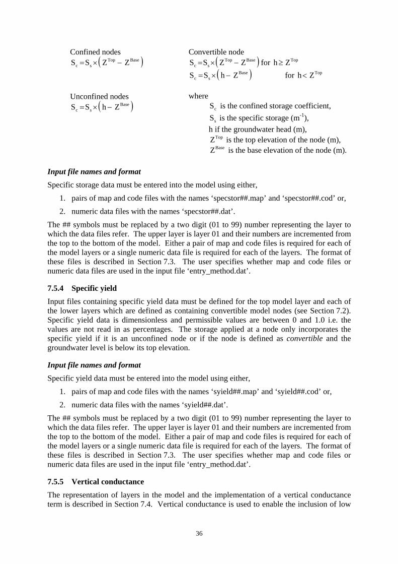
36
Confined nodes ( )BaseTop
sc ZZSS −×=
Unconfined nodes
( )Basesc ZhSS −×=
Convertible node ( )BaseTop
sc ZZSS −×= for TopZh ≥ ( )Base
sc ZhSS −×= for TopZh < where cS is the confined storage coefficient, sS is the specific storage (m-1), h if the groundwater head (m), TopZ is the top elevation of the node (m), BaseZ is the base elevation of the node (m).
Input file names and format Specific storage data must be entered into the model using either,
1. pairs of map and code files with the names ‘specstor##.map’ and ‘specstor##.cod’ or,
2. numeric data files with the names ‘specstor##.dat’.
The ## symbols must be replaced by a two digit (01 to 99) number representing the layer to which the data files refer. The upper layer is layer 01 and their numbers are incremented from the top to the bottom of the model. Either a pair of map and code files is required for each of the model layers or a single numeric data file is required for each of the layers. The format of these files is described in Section 7.3. The user specifies whether map and code files or numeric data files are used in the input file ‘entry_method.dat’.
7.5.4 Specific yield
Input files containing specific yield data must be defined for the top model layer and each of the lower layers which are defined as containing convertible model nodes (see Section 7.2). Specific yield data is dimensionless and permissible values are between 0 and 1.0 i.e. the values are not read in as percentages. The storage applied at a node only incorporates the specific yield if it is an unconfined node or if the node is defined as convertible and the groundwater level is below its top elevation.
Input file names and format
Specific yield data must be entered into the model using either,
1. pairs of map and code files with the names ‘syield##.map’ and ‘syield##.cod’ or,
2. numeric data files with the names ‘syield##.dat’.
The ## symbols must be replaced by a two digit (01 to 99) number representing the layer to which the data files refer. The upper layer is layer 01 and their numbers are incremented from the top to the bottom of the model. Either a pair of map and code files is required for each of the model layers or a single numeric data file is required for each of the layers. The format of these files is described in Section 7.3. The user specifies whether map and code files or numeric data files are used in the input file ‘entry_method.dat’.
7.5.5 Vertical conductance The representation of layers in the model and the implementation of a vertical conductance term is described in Section 7.4. Vertical conductance is used to enable the inclusion of low
37
permeability layers between aquifers, in which flow is assumed to be predominantly vertical, without having to incorporate additional numerical layers of finite difference nodes.
Input file names and format The vertical conductance between finite difference nodes in adjacent layers must be entered into the model using either,
1. pairs of map and code files with the names ‘vcond##.map’ and ‘vcond##.cod’ or,
2. numeric data files with the names ‘vcond##.dat’.
The ## symbols must be replaced by a two digit (01 to 99) number representing the layer to which the data files refer. The upper layer is layer 01 and layer numbers are incremented from the top to the bottom of the model. Either a pair of map and code files is required for each of the model layers or a single numeric data file is required for each of the layers. The format of these files is described in Section 7.3. The user specifies whether map and code files or numeric data files are used in the input file ‘entry_method.dat’.
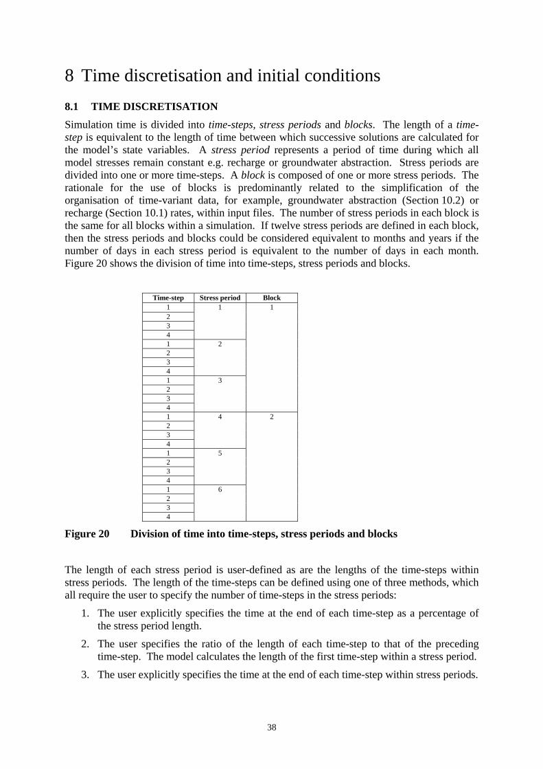
38
8 Time discretisation and initial conditions 8.1 TIME DISCRETISATION Simulation time is divided into time-steps, stress periods and blocks. The length of a time-step is equivalent to the length of time between which successive solutions are calculated for the model’s state variables. A stress period represents a period of time during which all model stresses remain constant e.g. recharge or groundwater abstraction. Stress periods are divided into one or more time-steps. A block is composed of one or more stress periods. The rationale for the use of blocks is predominantly related to the simplification of the organisation of time-variant data, for example, groundwater abstraction (Section 10.2) or recharge (Section 10.1) rates, within input files. The number of stress periods in each block is the same for all blocks within a simulation. If twelve stress periods are defined in each block, then the stress periods and blocks could be considered equivalent to months and years if the number of days in each stress period is equivalent to the number of days in each month. Figure 20 shows the division of time into time-steps, stress periods and blocks.
Time-step Stress period Block
1 2 3 4
1
1 2 3 4
2
1 2 3 4
3
1
1 2 3 4
4
1 2 3 4
5
1 2 3 4
6
2
Figure 20 Division of time into time-steps, stress periods and blocks
The length of each stress period is user-defined as are the lengths of the time-steps within stress periods. The length of the time-steps can be defined using one of three methods, which all require the user to specify the number of time-steps in the stress periods:
1. The user explicitly specifies the time at the end of each time-step as a percentage of the stress period length.
2. The user specifies the ratio of the length of each time-step to that of the preceding time-step. The model calculates the length of the first time-step within a stress period.
3. The user explicitly specifies the time at the end of each time-step within stress periods.

39
If the second method is implemented then the length of the time-steps are calculated using the following expressions
( )n
SP
1 11tt
α−α−×Δ
=Δ
1ii tt −Δ×α=Δ
where
itΔ is the length of the ith time-step, SPtΔ is the length of the stress period,
α is the time-step length multiplier,
n is the number of time-steps in each stress period.
8.1.1 Input file format
The discretisation of time is specified using an input file with the structure shown in Figure 21. The name of this file is fixed and must be ‘clock.dat’. The file defines the discretisation of time in the model, the frequency of some model output, whether the simulation is a steady-state or time-variant run, whether the model is being re-run using a condition simulated in a previous model run and, whether flow and head information is output to enable subsequent particle tracking simulations to be performed.
The input file contains comment lines, which describe the data on subsequent lines. These comment lines or text strings must be included in the input file but are read and discarded by the program. For reference purposes only, a line number is shown in the first column of Figure 21. This column is not part of the input file.
The discretisation of time is specified between lines 1 and 18. The number of time-steps per stress period, stress periods per block, and blocks are selected in addition to the length of each stress period. On line 6 the user specifies the time at the start of the simulation, which does not necessarily have to correspond to the stress period and block numbers. If the user specifies that stress periods and blocks are equivalent to months and years (line 10), the program checks that the length of each stress period is equal to the number of days in each month. In this case the user must ensure that,
1. there are twelve stress periods per block (line 2) and that
2. the time at the end of the penultimate time-step is less than 28 days (i.e. less than the number of days in February) if method 1 or 3 is selected for calculating the time-step lengths (line 14 or 18).
The program automatically corrects for leap years.
Between lines 20 and 24 the block numbers are listed. Blocks numbers can be listed out of sequence or repeated, except when recharge data is input using the numeric data file discussed in Section 10.1.2.
On line 26 an integer flag is entered which specifies the frequency of data output. The group of files ‘accretion.out’, ‘contour.txt’, ‘finalh.out’, ‘flowbal.out’, ‘global.out’ and ‘riverflow.out’, may be rewritten after every time-step, stress period or block, or only at the end of the simulation. The model runs more quickly if data is output less often and it is

40
recommended that this integer is generally set to 4. However, the ability to output data after every time-step, for example, means that if a simulation is aborted for any reason it can be re-started from a later time, thus reducing the subsequent run-time. The output files listed above are described in detail in Part 3 of this manual.
On line 28 a character flag specifies whether the simulation is a steady-state or time-variant run. If a steady-state simulation is selected, the storage coefficient is set to zero at all nodes of the mesh. In this case the model simulates a single time-step only. If rivers, springs or unconfined conditions are incorporated in the model, steady-state conditions must be approached by simulating multiple time-steps with constant stresses. This means that a ‘t’ must be entered on line 28 and that specific storage and specific yield must be specified using the relevant input files.
On line 30 of the example ‘clock.dat’ input file a character flag (‘y’ or ‘n’) is entered which specifies if initial the groundwater head profile is read from the file ‘initialh.dat’, described in Section 8.2. This file has the same format as one of ZOOMQ3D output files and contains the value of groundwater head at each node in the model. If the flag is equal to ‘y’ this file is opened and read. This enables simulations to re-run from a previously simulated condition.
On the last line of the input file the user specifies if information is to be output which enables particle tracking simulations to be run. If the user does wish to track particles then two additional output files are produced, ‘heads.txt’ and ‘flows.txt’, which are required by the particle tracking code ZOOPT for input.

41
Line Example ‘clock.dat’ file
1 2 3 4 5 6 7 8 9 10 11 12 13 14 15 16 17 18 19 20 21 22 23 24 25 26 27 28 29 30 31 32
// Number of time-steps, stress periods and blocks 4 12 5 // Number of the stress period and block after which to terminate simulation 12 5 // Enter start time of simulation year, month, day, hh:mm:ss 1970 1 1 00:00:00 // Length of each of the stress periods in the blocks 31.0 28.0 31.0 30.0 31.0 30.0 31.0 31.0 30.0 31.0 30.0 31.0 // Stress periods and blocks represent months and years? (y or n) y // Method of calculating time-step length (1, 2 or 3) 3 // Data for method 1: % of stress period length at end of time-step 1 to (number of time-steps -1) 10.0 25.0 50.0 // Data for method 2: Geometric progression - time-step multiplier 1.5 // Data for method 3: Specified time at end of time-step 1 to (number of time-steps -1) 4.0 10.0 18.0 // Block number order - one per line for each block 1970 1971 1972 1973 1974 // Data output at end of every time-step(1), stress period(2), block(3), or only at end of simulation(4) 4 // Steady-state or time-variant? (s or t) t // Rerunning? (y or n) n // Output particle tracking info? (y or n) n
Figure 21 Example ‘clock.dat’ file

42
8.2 INITIAL GROUNDWATER HEADS Initial groundwater heads can be entered into the model using two different methods. These methods employ either
1. a pair of map and code input files for each layer with the names ‘initialh##.map’ and ‘initialh##.cod’or,
2. a single numeric input data file containing initial groundwater heads for the whole model. (Note that this file does not have the same format as the numeric files for defining other spatially variable model parameter values).
When using the map and code files to input initial groundwater heads, the ## symbols must be replaced by a two digit (01 to 99) number representing the layer to which the data files refer. The upper layer is layer 01 and their numbers are incremented from the top to the bottom of the model. The format of these map and code files is described in Section 7.3.
Initial groundwater heads can also be defined using a single input file, the name of which is specified by the user in the input file ‘zoomq3d.dat’. This has the same format as one of the ZOOMQ3D output files, whose name is also specified in the input file ‘zoomq3d.dat’. Consequently, the output file can be used to start a simulation using the groundwater heads computed at the end of a previous run. The format of this input and output file is shown in Figure 22.
Base
grid
Grid 1
Subgrid
2
Layer 01
Base
Grid
Subgrid
1
INITIAL GROUNDWATER HEADS ********** LAYER 01 ********** **** BASE GRID **** -------------------------------------------- | Replace rectangle with an array of initial | | groundwater heads with the same number of | | rows and columns as this grid | -------------------------------------------- **** SUBGRID 1 **** -------------------------------------------- | Replace rectangle with an array of initial | | groundwater heads with the same number of | | rows and columns as this grid | -------------------------------------------- **** SUBGRID 2 **** -------------------------------------------- | Replace rectangle with an array of initial | | groundwater heads with the same number of | | rows and columns as this grid | -------------------------------------------- ********** LAYER 02 ********** **** BASE GRID **** -------------------------------------------- | Replace rectangle with an array of initial | | groundwater heads with the same number of | | rows and columns as this grid | -------------------------------------------- **** SUBGRID 1 **** -------------------------------------------- | Replace rectangle with an array of initial | | groundwater heads with the same number of | | rows and columns as this grid | -------------------------------------------- **** SUBGRID 2 **** -------------------------------------------- | Replace rectangle with an array of initial | | groundwater heads with the same number of | | rows and columns as this grid | --------------------------------------------
Subgrid
2
Layer 02
Figure 22 Format of numeric initial groundwater head data file

43
The first line of the file is a comment line. Blocks of data follow this comment line for each model layer, starting with the top layer. Within each block of layer data, blocks of data are defined for the base grid and for each refined grid within the model. The grid data blocks are listed in the same order as those in the map and code files, or dat files, in which other spatially varying model parameters are specified (see Section 7.3). Data for the base grid are always entered at the start of a layer block. The first line of each layer block is a comment line and the first line of each grid block is a comment line.
After the comment line at the start of each grid data block, an array of groundwater head values is entered. This array must have the same number of rows and columns as the finite difference grid to which it relates i.e. the base grid or one of the refined grids. The first line of the array of head values relates to the top (furthest in the positive y-direction) row of the grid. Some points on a grid may be located outside the model boundary, however, a groundwater head value must be entered in all elements of the rectangular array, or matrix, of grid points. The values corresponding to nodes located outside the model boundary are read but ignored.
44
9 Boundary conditions 9.1 MODEL EDGE BOUNDARY CONDITIONS Boundary conditions around the edge of the model are specified using the file ‘boundary.dat’. This file is produced by ZETUP but may require modification before being used as a ZOOMQ3D input file. The file is used to assign each finite difference node on the boundary of the model a fixed head value or a fixed inflow rate that will be applied during the simulation. Each node located on the boundary of the model is listed in this file, which consists of multiple lines of text with the following format x y BC1 BCV1 BC2 BCV2 BC3 BCV3 ……………… BCi BCVi
where
x is the x co-ordinate of the boundary node,
y is the y co-ordinate of the boundary node,
BCi is a character flag. It is set to ‘s’ to indicate that the boundary node is a specified
inflow node and to ‘f’ to specify a fixed head node,
BCVi is either the inflow rate (m3 day-1) or the fixed head value (m),
i represents the model layer number (i = 1 to the number of model layers).
The nodes are listed in the file in an order defined by a clockwise movement around the boundary. A termination line must be included at the end of the file which contains two numbers whose values are negative one, that is -1.0 –1.0
9.2 INTERNAL FIXED HEADS
Fixed head nodes inside of the model boundary are defined in a file with the following structure. The name of this file is specified by the user in the input file ‘zoomq3d.dat’. The file has the format n
layer x y h (one line for each of the n nodes)
where
n is the number of fixed head nodes specified in the file,
layer is the number of the model layer,
x is the x co-ordinate of the fixed head,
y is the y co-ordinate of the fixed head,
h is the elevation of the fixed head (m).
If nodes are specified in this file that duplicate those in ‘boundary.dat’, then they will be ignored. The conditions specified in ‘boundary.dat’ take precedence over those specified in this input file.
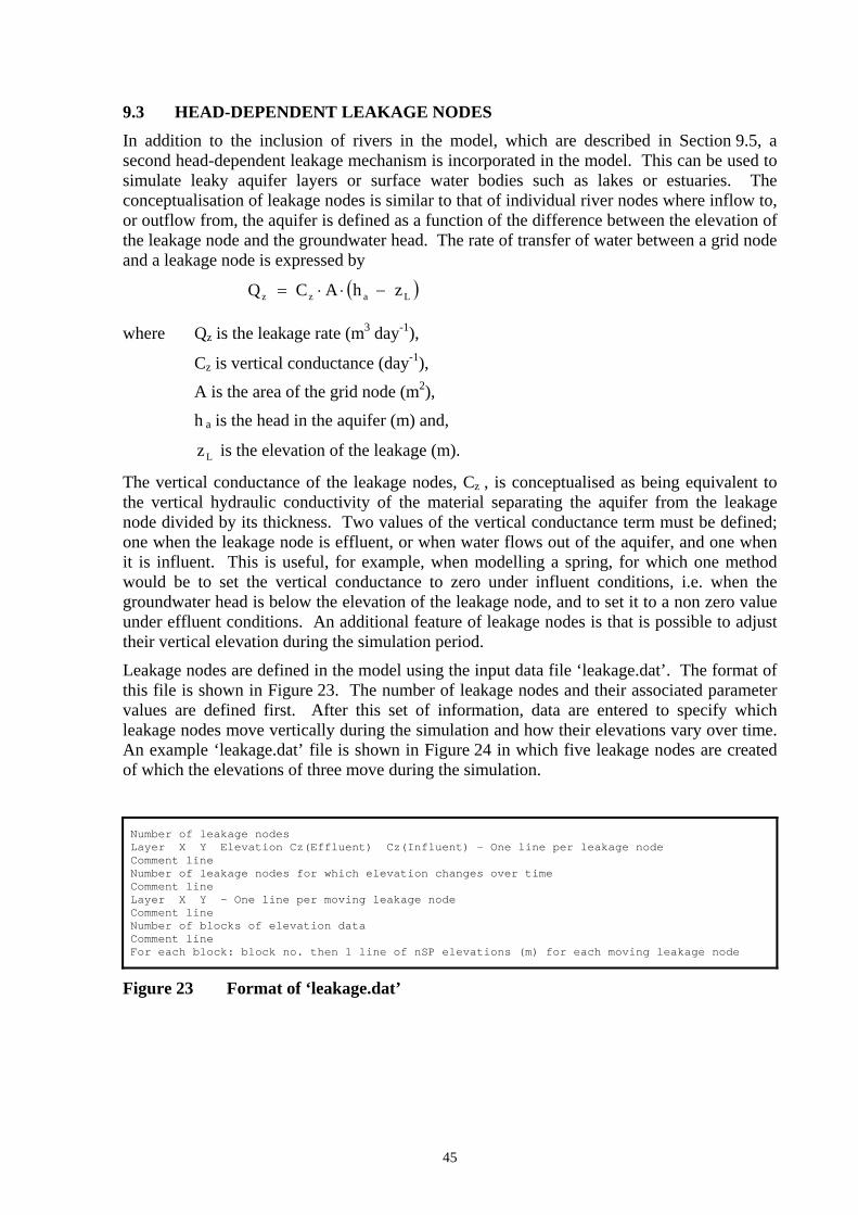
45
9.3 HEAD-DEPENDENT LEAKAGE NODES In addition to the inclusion of rivers in the model, which are described in Section 9.5, a second head-dependent leakage mechanism is incorporated in the model. This can be used to simulate leaky aquifer layers or surface water bodies such as lakes or estuaries. The conceptualisation of leakage nodes is similar to that of individual river nodes where inflow to, or outflow from, the aquifer is defined as a function of the difference between the elevation of the leakage node and the groundwater head. The rate of transfer of water between a grid node and a leakage node is expressed by
( )Lazz zhACQ −⋅⋅=
where Qz is the leakage rate (m3 day-1),
Cz is vertical conductance (day-1),
A is the area of the grid node (m2),
h a is the head in the aquifer (m) and,
Lz is the elevation of the leakage (m).
The vertical conductance of the leakage nodes, Cz , is conceptualised as being equivalent to the vertical hydraulic conductivity of the material separating the aquifer from the leakage node divided by its thickness. Two values of the vertical conductance term must be defined; one when the leakage node is effluent, or when water flows out of the aquifer, and one when it is influent. This is useful, for example, when modelling a spring, for which one method would be to set the vertical conductance to zero under influent conditions, i.e. when the groundwater head is below the elevation of the leakage node, and to set it to a non zero value under effluent conditions. An additional feature of leakage nodes is that is possible to adjust their vertical elevation during the simulation period.
Leakage nodes are defined in the model using the input data file ‘leakage.dat’. The format of this file is shown in Figure 23. The number of leakage nodes and their associated parameter values are defined first. After this set of information, data are entered to specify which leakage nodes move vertically during the simulation and how their elevations vary over time. An example ‘leakage.dat’ file is shown in Figure 24 in which five leakage nodes are created of which the elevations of three move during the simulation.
Number of leakage nodes Layer X Y Elevation Cz(Effluent) Cz(Influent) – One line per leakage node Comment line Number of leakage nodes for which elevation changes over time Comment line Layer X Y – One line per moving leakage node Comment line Number of blocks of elevation data Comment line For each block: block no. then 1 line of nSP elevations (m) for each moving leakage node
Figure 23 Format of ‘leakage.dat’

46
5 1 8000.0 3250.0 6.0 10.0 0.0 1 9000.0 3000.0 6.0 10.0 0.0 1 9250.0 3000.0 6.0 10.0 0.0 1 9500.0 3000.0 6.0 10.0 0.0 1 9750.0 3000.0 5.0 10.0 0.0 // Number of nodes for which elevation changes during simulation 3 // Layer, X and Y co-ordinate of each moving node 1 9250.0 3000.0 1 9500.0 3000.0 1 9750.0 3000.0 // Number of years of elevation data 5 // For each block: year no. then 1 line of nSP elevations (m) for each moving leakage node 1970 6.0 6.0 6.0 6.0 6.0 6.0 6.0 6.0 6.0 6.0 6.0 6.0 6.0 6.0 6.0 6.0 6.0 6.0 6.0 6.0 6.0 6.0 6.0 6.0 5.0 5.0 5.0 5.0 5.0 5.0 5.0 5.0 5.0 5.0 5.0 5.0 1971 6.0 6.0 6.0 6.0 6.0 6.0 6.0 6.0 6.0 6.0 6.0 6.0 6.0 6.0 6.0 6.0 6.0 6.0 6.0 6.0 6.0 6.0 6.0 6.0 5.0 5.0 5.0 5.0 5.0 5.0 5.0 5.0 5.0 5.0 5.0 5.0 1972 5.0 5.0 5.0 5.0 5.0 5.0 5.0 5.0 5.0 5.0 5.0 5.0 5.0 5.0 5.0 5.0 5.0 5.0 5.0 5.0 5.0 5.0 5.0 5.0 5.0 5.0 5.0 5.0 5.0 5.0 5.0 5.0 5.0 5.0 5.0 5.0 1973 5.0 5.0 5.0 5.0 5.0 5.0 5.0 5.0 5.0 5.0 5.0 5.0 5.0 5.0 5.0 5.0 5.0 5.0 5.0 5.0 5.0 5.0 5.0 5.0 4.0 4.0 4.0 4.0 4.0 4.0 4.0 4.0 4.0 4.0 4.0 4.0 1974 4.0 4.0 4.0 4.0 4.0 4.0 4.0 4.0 4.0 4.0 4.0 4.0 3.0 3.0 3.0 3.0 3.0 3.0 3.0 3.0 3.0 3.0 3.0 3.0 3.0 3.0 3.0 3.0 3.0 3.0 3.0 3.0 3.0 3.0 3.0 3.0
Figure 24 Example ‘leakage.dat’ file
9.3.1 Monitoring flow through leakage nodes over time The flows into and out of leakage nodes are monitored over time by specifying data in a file with the following structure. The name of this file, for example ‘obsleak.dat’, is specified by the user in the input file ‘zoomq3d.dat’ (see Section 14.2). The file has the format n
start_block end_block
Layer x y (one for each of n leakage nodes)
where
n is the number of leakage nodes at which the flow is monitored,
start_block is the block number when monitoring starts,
end_block is the block number when monitoring ends,
Layer is the layer in which the leakage node has been created,
x is the x co-ordinate of the leakage node and,
y is the y co-ordinate of the leakage node.

47
9.4 SPRINGS
9.4.1 Conceptualisation Springs are usually simulated in models using a head-dependent leakage mechanism. This mechanism is incorporated in the model, however, the conceptualisation of a spring in this way, in which the outflow from the aquifer is based on a ‘bed conductance’ could be argued to be simplistic. Consequently, a spring mechanism has been developed in which spring flows are dependent on the groundwater head in the aquifer, but not governed by a conductance term. Instead, spring flows can only be adjusted by modifying the transmissivity of the aquifer in the region of the spring. Consequently, the general pattern of flow within the aquifer determines the outflow at a spring location.
Springs in ZOOMQ3D encapsulate a head-dependent abstraction mechanism. When simulating unconfined aquifers the transmissivity is updated within a cyclical procedure (see Section 7.2.2). The solution for the current time-step is computed a number of times within this cyclical process. After each cycle the transmissivity is adjusted. Spring flows are also adjusted at the end of each cycle. A spring object is defined by an upper and lower elevation, which for example, represent the ground level and a level just below the ground surface, e.g. 0.1 m below the ground surface. If at the end of a cycle the groundwater head at this node is above the upper spring elevation then the spring is set to a fixed flow. This flow rate is calculated, using the specific yield and time-step length, so that the groundwater head is lowered to between the two elevations defined in the spring object. It is given by the equation
( )t
yxS2
ZZhQ yTBs Δ
Δ×Δ××⎥⎦
⎤⎢⎣⎡ +
−=
where
sQ is the specified spring flow rate (m3 day-1),
h is the groundwater head at the spring node (m),
TZ is the elevation of the top of the spring (m),
BZ is the elevation of the base of the spring (m),
xΔ is the width of the node in the x-direction (m),
yΔ is the width of the node in the x-direction (m),
yS is the specific yield and,
tΔ is the time-step length (days).
Consequently, the spring is set to ‘abstract’ water from the aquifer during the next cycle of the transmissivity/spring flow adjustment procedure. At the end of the next cycle the spring flow is readjusted by examining the groundwater head again. This cyclical procedure terminates and the simulation progresses to the next time-step when both the transmissivity and spring flows stop varying between cycles. If the groundwater head is simulated to be below the base of the spring, its flows rate is set to zero.

48
9.4.2 Input file format Springs are defined in the model using the file ‘springs.dat’. The name of this file is invariable. Springs can only be placed in the top model layer at unconfined or convertible nodes. The input file has the following structure. n
x y ZT ΔZ (one line for each of n springs)
where
n is the number of springs,
x is the x co-ordinate of the spring (m),
y is the y co-ordinate of the spring (m),
ZT is the elevation of the top of the spring (m) and,
ΔZ is the depth of the spring (m)
The base elevation of the spring is calculated by subtracting the spring depth from the top elevation. An example ‘springs.dat’ input file is shown in Figure 25.
5 0.0 4000.0 15.0 0.1 500.0 3500.0 15.0 0.1 500.0 3000.0 15.0 0.1 1000.0 2500.0 15.0 0.1 1500.0 1500.0 15.0 0.1
Figure 25 Example ‘springs.dat’ input file

49
9.5 RIVERS ZOOMQ3D can simulate baseflow within dendritic river basins. Both the baseflow along the river and the interaction between the river and the aquifer can be modelled. The structure of rivers within ZOOMQ3D is described using three terms: rivers, branches and river nodes, which have the following definition:
Rivers: a river is composed of both an interconnected series of river branches and a interconnected series of river nodes. A river cannot be composed of two sets of interconnected river nodes that are not themselves connected, i.e. a river cannot represent multiple separate catchments.
Branch: a branch represents the main channel in a catchment or a tributary within the river (catchment). Only dendritic river catchments can be modelled and consequently, each branch has one node at its upstream end and one node at its downstream end.
River node: a river node represents a point on the river that coincides with a horizontal point of the finite difference mesh. The characteristics of the river are defined at each river node. A river node can have up to five upstream connections to river nodes but only one downstream connection.
Branches and river nodes are organised in a specific order described by a numbering scheme. For river branches a numbering scheme must be adopted in which the upstream branches have a higher integer value (Figure 26a). River node numbers also increase upstream and from low branch numbers to high branch numbers (Figure 26b). The river node at the bottom of the catchment must be number 1.

50
1
1
1
1
2
2
3
4
5
15
1
2
4
3
6
5
34
37
35
36
38 39
40
7
8
9
7310 72 74
13
14
11
12
75
94
95
96
97
98
1691
92
90
93
17 18
100 99
85 86 7155
60
54
4341 42
44
45 46
77
78
79
80
82
76
81 83 84
48
47
57
49
58
59
50
51
52
53
67
70
61 62 63
64
65
66
68
69
19
20
23
25
21 22
24
26 27
87
88
89
30
29
28
31
32
33
56
(a) (b)
Figure 26 Numbering schemes in ZOOMQ3D for (a) river branches and (b) river nodes for an example model river

51
Figure 27 Schematic representation of connections between river and grid nodes
As stated above, rivers are represented by a series of linked river nodes, which are also connected with upper most active aquifer node as illustrated in Figure 27. Each river node is located at the centre of the reach that it represents. The limits of a reach are the midpoints between the central river node and its adjacent river nodes. River nodes are characterised by the following set of parameters:
• Location specified by x and y co-ordinates (m).
• Width (m).
• Reach length (m). Equivalent to the half the straight line distance between the adjacent two river nodes.
• River stage (m).
• River-bed elevation (m).
• River-bed thickness (m).
• Vertical hydraulic permeability under effluent conditions (m day-1).
• Vertical hydraulic permeability under influent conditions (m day-1).
9.5.1 Conceptualisation of river-aquifer interaction In ZOOMQ3D river-aquifer interaction is represented as a linear head-dependent leakage mechanism. The rate of leakage depends on the difference between groundwater head and river stage and is expressed by
( )raz
z hhLWB
KQ −⋅⋅⋅=
where
Qz is the leakage rate (m3day-1),
Upper most active finite difference node
Interconnected river nodes
River-aquifer interaction
Baseflow
Baseflow
Baseflow

52
Kz is the vertical hydraulic conductivity of the river bed (m day-1),
B is the thickness of the river bed (m),
W is the width of the river (m),
L is the length of the river reach (m),
h a is the head in the aquifer (m) and,
h r is the river stage (m).
This equation is modified when the head in the aquifer falls below the base of the river bed, ( )BZBOT − , where BOTZ is the elevation of the bed of the river. Under these conditions, the driving head is equal to the difference between the river stage and the base of the river bed, ( )BZBOT − . The leakage from the river under perched conditions is therefore defined as
( )[ ]rBOTZ
z hBZLWB
KQ −−⋅⋅⋅=
In addition to limiting the flow between the aquifer and the river when the groundwater head falls below the river-bed, different hydraulic conductivity values are applied between influent and effluent conditions. The difference reflects the seepage force applied to the bed material and the associated increase in permeability when groundwater is discharging to the river. The hydraulic conductivities are defined by the user in input file ‘rivers.dat’. The different relative positions of the river stage and groundwater head are shown in Figure 28. The appropriate vertical flow equation representing the interaction is presented next to each scenario.
9.5.2 River input file
This file is created by ZETUP as ‘rivers.out’. For input into ZOOM2D is must be renamed ‘rivers.dat’. It contains parameter information for the river nodes which make up each river in the model. The file format is shown in Figure 30. This figure is based on the start of the ‘rivers.dat’ file used to construct the river shown in Figure 26.
Each river node is described by a four line block of data. The first line of the block is a series of dashes, which are used to separate each group of river node information. The second and fourth lines of the block should not be altered. The following parameters are listed on the third line of the block
i) the river stage (m),
ii) the river bed elevation (m),
iii) the channel width (m),
iv) the reach length (m),
v) the hydraulic conductivity of the river bed under effluent conditions (m day-1),
vi) the hydraulic conductivity of the river bed under influent conditions and (m day-1),
vii) the river-bed thickness (m).
All of the parameters can be altered by the user. However, the reach length should be considered fixed as it is defined by the distance between adjacent river nodes.
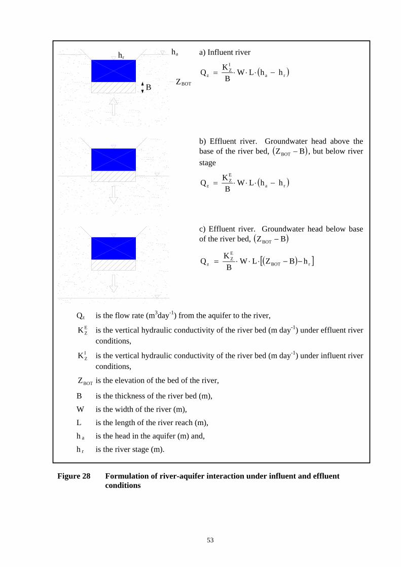
53
a) Influent river
( )ra
IZ
z hhLWB
KQ −⋅⋅⋅=
b) Effluent river. Groundwater head above the base of the river bed, ( )BZBOT − , but below river stage
( )ra
EZ
z hhLWB
KQ −⋅⋅⋅=
c) Effluent river. Groundwater head below base of the river bed, ( )BZBOT −
( )[ ]rBOT
EZ
z hBZLWB
KQ −−⋅⋅⋅=
Qz is the flow rate (m3day-1) from the aquifer to the river, EZK is the vertical hydraulic conductivity of the river bed (m day-1) under effluent river
conditions, IZK is the vertical hydraulic conductivity of the river bed (m day-1) under influent river
conditions,
BOTZ is the elevation of the bed of the river,
B is the thickness of the river bed (m),
W is the width of the river (m),
L is the length of the river reach (m),
h a is the head in the aquifer (m) and,
h r is the river stage (m).
Figure 28 Formulation of river-aquifer interaction under influent and effluent conditions
harh
BZBOT

54
9.5.3 Initial river flows This file is created by ZETUP and referred to as ‘initialflow.dat’ in this manual. It may be given any name providing this is entered into the input file ‘zoomq3d.dat’. The file contains information relating to the initial flow in the rivers at each of their nodes. The format of the file is shown in Figure 31 based on the river shown in Figure 26. Only the parameter values shown in bold should be modified by the user. These flows will determine how much water can leak into the aquifer during the first time-step if sections of the river run dry, for example, due to groundwater abstraction.
9.5.4 Time-variant inflows or discharges to rivers To specify time-variant discharges to a river, for example from a sewage treatment works, or to specify the baseflow in a river as it comes onto a model, as illustrated in Figure 29, the following file is used. The name of this file, for example ‘river_inputs.dat’, is specified by the user in the input file ‘zoomq3d.dat’ (see Section 14.2). It contains data specifying which river nodes receive baseflow and how these flows vary over time. An example file and a description of the file format is given in Figure 32. The user enters the following data:
• The number of river nodes at which an inflow is specified.
• The location of each of the river nodes defined by the river number and river node number.
• The number of time blocks for which flow rates are read.
• The inflow at each of the river nodes for each stress period in each time block.
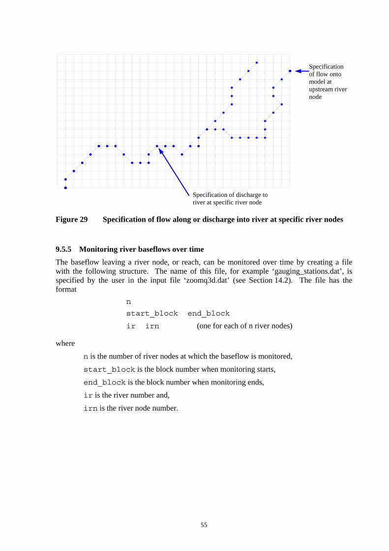
55
Figure 29 Specification of flow along or discharge into river at specific river nodes
9.5.5 Monitoring river baseflows over time The baseflow leaving a river node, or reach, can be monitored over time by creating a file with the following structure. The name of this file, for example ‘gauging_stations.dat’, is specified by the user in the input file ‘zoomq3d.dat’ (see Section 14.2). The file has the format n
start_block end_block
ir irn (one for each of n river nodes)
where
n is the number of river nodes at which the baseflow is monitored,
start_block is the block number when monitoring starts,
end_block is the block number when monitoring ends,
ir is the river number and,
irn is the river node number.
Specification of flow onto model at upstream river node
Specification of discharge to river at specific river node

56
‘rivers.dat’ Format of data
REPEATED FOR EACH RIVER
1
----------------------------------
river1_map.dat
1 100 5
-------------------
1 1 1500.0 0.0
1.0 0.0 5.0 125.0 0.1 0.05 1.0
1 2
-------------------
2 1 1500.0 250.0
1.0 0.0 5.0 301.77 0.1 0.05 1.0
1 3
-------------------
3 1 1750.0 500.0
1.06 0.06 5.0 353.55 0.1 0.05 1.0
1 4
etc for each node in the river
Number of rivers in the model
Comment line separator between data relating to each river
Name of the river map file used to create the model river (see ZETUP manual)
River number (unique identifier), number of river nodes, number of branches
Comment line separator between data relating to each river
River node number, Branch number, x co-ordinate, y co-ordinate
Stage, bed elevation, width, reach length, Kz(influent), Kz(influent), bed thickness
Number of upstream nodes connections, River node number of each upstream river node
Comment line separator between blocks of river node data
REPEATED FOR
EACH
RIVER NODE
Comment line separator between blocks of river node data
REPEATED FOR
EACH
RIVER NODE
Figure 30 Format of file ‘rivers.dat’
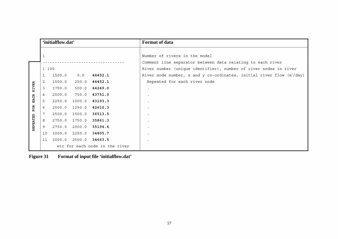
57
‘initialflow.dat’ Format of data
REPEATED FOR EACH RIVER
1
----------------------------------
1 100
1 1500.0 0.0 44452.1
2 1500.0 250.0 44452.1
3 1750.0 500.0 44249.0
4 2000.0 750.0 43751.0
5 2250.0 1000.0 43193.3
6 2500.0 1250.0 42610.3
7 2500.0 1500.0 36513.5
8 2750.0 1750.0 35861.3
9 2750.0 2000.0 35194.4
10 3000.0 2250.0 34805.7
11 3000.0 2500.0 34663.5
etc for each node in the river
Number of rivers in the model
Comment line separator between data relating to each river
River number (unique identifier), number of river nodes in river
River node number, x and y co-ordinates, initial river flow (m3/day)
Repeated for each river node
.
.
.
.
.
.
.
.
.
Figure 31 Format of input file ‘initialflow.dat’

58
‘river_inputs.dat’ Format of data
// Number of nodes at which specified time-variant discharge to river
2
// River number and node number for each
1 11
2 15
// Number of block time periods of discharge data
5
// For each block: block no. then 1 line of nSPs of flow rates (m3/day) for each node
1970
7602.8 6692.0 5879.9 3917.0 2739.3 1989.3 1637.6 2214.4 3221.4 5262.7 7107.3 7501.1
30411.0 26768.0 23519.7 15668.1 10957.3 7957.3 6550.3 8857.4 12885.6 21050.9 28429.4 30004.5
1971
7602.8 6692.0 5879.9 3917.0 2739.3 1989.3 1637.6 2214.4 3221.4 5262.7 7107.3 7501.1
30411.0 26768.0 23519.7 15668.1 10957.3 7957.3 6550.3 8857.4 12885.6 21050.9 28429.4 30004.5
1972
7602.8 6692.0 5879.9 3917.0 2739.3 1989.3 1637.6 2214.4 3221.4 5262.7 7107.3 7501.1
30411.0 26768.0 23519.7 15668.1 10957.3 7957.3 6550.3 8857.4 12885.6 21050.9 28429.4 30004.5
1973
7602.8 6692.0 5879.9 3917.0 2739.3 1989.3 1637.6 2214.4 3221.4 5262.7 7107.3 7501.1
30411.0 26768.0 23519.7 15668.1 10957.3 7957.3 6550.3 8857.4 12885.6 21050.9 28429.4 30004.5
1974
7602.8 6692.0 5879.9 3917.0 2739.3 1989.3 1637.6 2214.4 3221.4 5262.7 7107.3 7501.1
30411.0 26768.0 23519.7 15668.1 10957.3 7957.3 6550.3 8857.4 12885.6 21050.9 28429.4 30004.5
etc for each time block
Comment line
No. of nodes at which an input is specified
Comment line
River number, river node number
One line per number specified on line 2
Comment line
Number of block time periods of data
Comment line
Block number
Flow rate for each stress period for 1st node
Flow rate for each stress period for 2nd node
-- Repeated for each block
Discharge rates in m3/day
-- Repeated for each block
Discharge rates in m3/day
-- Repeated for each block
Discharge rates in m3/day
-- Repeated for each block
Discharge rates in m3/day
Figure 32 Format of input file ‘river_inputs.dat’

59
10 Model stresses 10.1 RECHARGE The specification of recharge is perhaps the most complex of tasks within ZOOMQ3D. However, the data input files are not themselves complex. The spatial and temporal distribution of recharge can be specified using two methods:
1. The use of map and code files similar to those described in Section 7.3.
2. The use of a single numeric data file containing arrays of recharge rates in mm day-1.
In fact both of these methods can be implemented simultaneously.
10.1.1 Applying recharge using map and code files
The formats of the recharge map and code files are identical to those described in Section 7.3. An example code file is shown in Figure 33 for a hypothetical model which contains a coarse base grid and no grid refinement. If this code file was related to the specification of hydraulic conductivity, a value of 0.9 m day-1 would be applied where an ‘a’ is located in the corresponding map file and a value of 1.2 m day-1 applied where a ‘b’ is defined. If this was a recharge code file, the values would not represent recharge rates of 0.9 and 1.2 mm day-1 but rather multipliers of a recharge rate defined in a file, for example named ‘recharge.dat’. The values in the code files are multipliers and not actual values of recharge because recharge varies both spatially and temporally. The spatial variation is defined using the map and code file and the temporal variation is defined within the file ‘recharge.dat’.
---- Code file ---- 2 0.9 1.2
---- Map file ---- aaaaaaaabbbbb aaaaaaaabbbbb aaaaaaaabbbbb
Figure 33 Example code and map file for the entry of recharge data
Recharge rates are specified in ‘recharge.dat’, for each stress period within the simulation. Actually the name ‘recharge.dat’ is just an example as it is defined by the user in the input file ‘zoomq3d.dat’. Consider that for ten consecutive stress periods the recharge rates shown in Table 4 are defined. Assuming that this data set relates to the code and map files shown in Figure 33, then during stress period 2, the recharge rate at the nodes represented by the letter ‘a’ would be 0.99 mm day-1 (0.9 × 1.1 mm day-1). During stress period 10 the recharge rate at the nodes represented by the letter ‘b’ would be 0.24 mm day-1 (1.2 × 0.2 mm day-1).
Table 4 Hypothetical recharge rates (mm day-1) for ten stress periods
Stress period 1 2 3 4 5 6 7 8 9 10
Recharge rate (mm day-1) 1.2 1.1 0.6 0.7 0.0 0.0 0.0 0.0 0.0 0.2
In ZOOMQ3D, the set of recharge data defined by a code file, a map file and a set of rates for each stress period in the simulation is referred to as a recharge type. This

60
terminology is adopted because more than one recharge type can be defined. The rationale for implementing multiple recharge types is best illustrated using an example.
Suppose the groundwater system shown in Figure 34 is to be modelled. This represents a slice through an aquifer from an interfluve in the west to a river valley in the east. The slice is 3 km long and over the western 2 km the aquifer is covered by low permeability deposits, which inhibit, but do not limit recharge. Assume that a conceptual model has been developed in which recharge over the western 2 km is considered to occur at a low but constant rate but in the east, where there is no superficial cover, recharge is higher and seasonally varying. Also assume a one-year period is to be simulated for which recharge rates have been defined on a monthly basis for both the covered and uncovered areas of the aquifer. These are listed in Table 5. The one-year simulation period is split into twelve stress periods.
Table 5 Hypothetical recharge rates (mm day-1) for monthly stress periods
Stress period 1 2 3 4 5 6 7 8 9 10 11 12
Covered interfluve area 0.1 0.1 0.1 0.1 0.1 0.1 0.1 0.1 0.1 0.1 0.1 0.1
Valley 1.2 1.1 0.7 0.5 0.0 0.0 0.0 0.0 0.0 0.1 0.6 1.1
Aquifer
Superficial deposits
West East
Figure 34 Example aquifer modelled using two recharge types
Figure 35 Example model mesh used to simulate aquifer shown in Figure 34
West
East
Uncovered aquifer nodes 250 m square mesh

61
The model mesh used to simulate this system is shown in Figure 35. The model is 3 km long in the west-east direction and 500 m wide in the south-north direction. In the horizontal the grid is composed of a regular 250 m square mesh, resulting in 39 nodes. The fifteen nodes closest to the eastern boundary represent the part of the aquifer not covered by superficial deposits. There is only one layer in the model but this is not of relevance.
This system could not be modelled using a single recharge type because of the different time series of recharge in the different areas. As stated previously, over the area of the aquifer covered by superficial deposits recharge is constant but it varies seasonal in the valley area. However, using two recharge types it is straightforward to represent this recharge pattern and simple to produce the required data files. The data contained in ‘recharge.dat’ and the code and map files for each recharge type are listed in Figure 36. It is apparent from examining recharge type 1 that this data set results in a constant recharge of 0.1 mm day-1 being applied to the interfluve area and no recharge in the valley. No recharge occurs in recharge type 2 over the area covered by superficial deposits but a time-varying recharge is applied to the uncovered aquifer. The recharge rates calculated in each recharge type are additive and so the scheme illustrated in Figure 34 produces the recharge pattern described by the conceptual model.
Recharge type 1 – superficial cover Recharge type 2 – uncovered aquifer
Stress period Recharge (mm day-1) Stress period Recharge
(mm day-1) Stress period Recharge (mm day-1) Stress period Recharge
(mm day-1)
1 0.1 7 0.1 1 1.2 7 0.0
2 0.1 8 0.1 2 1.1 8 0.0
3 0.1 9 0.1 3 0.7 9 0.0
4 0.1 10 0.1 4 0.5 10 0.1
5 0.1 11 0.1 5 0.0 11 0.6
Rec
harg
e ra
te d
ata
set
6 0.1 12 0.1 6 0.0 12 1.1
Cod
e fil
e ---- Code file 1 ---- 2 1.0 0.0
---- Code file 2 ---- 2 0.0 1.0
Map
file
---- Map file 1 ---- aaaaaaaabbbbb aaaaaaaabbbbb aaaaaaaabbbbb
---- Map file 2 ---- aaaaaaaabbbbb aaaaaaaabbbbb aaaaaaaabbbbb
Figure 36 Example recharge time series, recharge code file and recharge map file used to define two different recharge types

62
10.1.2 Applying recharge using a numeric data file The use of recharge types and associated map and code files is not obligatory. Instead a single numeric data file can be used containing arrays of recharge rates in mm day-1 for each stress period in the simulation. This numeric recharge file can also be used in conjunction with recharge map and code files. If both recharge data entry methods are used simultaneously the recharge rates defined by each are added together before being applied. The name of the numeric recharge file is specified by the user in the main recharge file, which is described in the next sub-section. The arrays contained in the numeric recharge file relate to each of the grids in the model. The format of the file is shown in Figure 37.
Recharge data is specified for each stress period of each simulation time block, in the time block order specified in ‘clock.dat’. Within each stress period, arrays of recharge data are defined for the base grid and for each refined grid within the model. The recharge arrays for each grid are listed in the same order as the grids in the map and code files, or dat files, in which other spatially varying model parameters are specified (see Section 7.3). Data for the base grid are always first for each stress period. The first line of each recharge array corresponding to a grid is a comment line and the first line of each stress period data set is the stress period number and time block number.
File format File structure Multiplier to convert rates to m day-1
Stress period and block number
Base grid
Subgrid 1
Subgrid 2
Stress period 1
Stress period and block number
Base Grid
Subgrid 1
0.001
1 1970 **** BASE GRID **** (Comment line) ----------------------------------------- | Replace rectangle with an array of | | recharge rates (mm/day) with the same | | number of rows and columns as this grid | ----------------------------------------- **** SUBGRID 1 **** (Comment line) ----------------------------------------- | Replace rectangle with an array of | | recharge rates (mm/day) with the same | | number of rows and columns as this grid | ----------------------------------------- **** SUBGRID 2 **** (Comment line) ----------------------------------------- | Replace rectangle with an array of | | recharge rates (mm/day) with the same | | number of rows and columns as this grid | ----------------------------------------- 2 1970 **** BASE GRID **** (Comment line) ----------------------------------------- | Replace rectangle with an array of | | recharge rates (mm/day) with the same | | number of rows and columns as this grid | ----------------------------------------- **** SUBGRID 1 **** (Comment line) ----------------------------------------- | Replace rectangle with an array of | | recharge rates (mm/day) with the same | | number of rows and columns as this grid | ----------------------------------------- **** SUBGRID 2 **** (Comment line) ----------------------------------------- | Replace rectangle with an array of | | recharge rates (mm/day) with the same | | number of rows and columns as this grid | -----------------------------------------
Subgrid 2
Stress period 2
etc for each stress period and for each grid within each stress period
Figure 37 Format of numeric recharge data file
This file format results in recharge rates being defined more than once at particular finite difference nodes when the model mesh is locally refined. This occurs at those nodes on a

63
refined grid that are coincident with the nodes on a coarser grid. Where this occurs the data defined on the refined grid will always override that defined on the coarse mesh. Some points on a grid may be located outside the model boundary, however, a recharge rate value must be entered in all elements of the rectangular array, or matrix, of grid points. The values corresponding to nodes located outside the model boundary are read but then ignored.
The ZOOM family recharge model, ZOODRM (Mansour and Hughes, 2004), creates a recharge file in this format.
10.1.3 The main recharge data file The name of the main recharge input file is specified by the user in the input file ‘zoomq3d.dat’. This file, for example ‘recharge.dat’, contains the time-series of recharge rates relating to each recharge type and the names of the associated map and code files. The user also specifies if a numeric data file is being used and if so its name. In summary the file is used to specify:
• if recharge types are used to specify recharge i.e. if map and code files are used,
• how many recharge type are being used,
• the names of the pair of map and code files associated with each recharge type,
• a recharge rate for each stress period for each recharge type in mm day-1,
• if a numeric data file is being used to specify recharge, as an alternative to, or in conjunction with the use of map and code files,
• the name of the numeric data file.
An example ‘recharge.dat’ file is shown in Figure 38. The first two lines of this file are a comment line and an integer flag. The integer flag determines whether recharge types, and their associated map and codes files, are to be used (1), whether the numeric recharge data file is to be used (2) or whether both methods of recharge specification are implemented (3).
The file is split into two sections after the first two lines. The first section must begin with a comment line starting ‘SECTION 1’ (Figure 38 – line 4) and the second section must begin with a comment line starting ‘SECTION 2’ (line 28). In the first section data is defined relating to the definition of recharge using recharge types. In the second section information is defined relating to the specification of recharge using a numeric data file.
In section 1 the number of recharge types being applied is specified (line 9). For each recharge type the name of the map and code file must be specified (lines 11-14). After this the number of time blocks of recharge data is entered (line 16). For each block, the block number is entered. This is followed by a line of recharge rates (mm day-1) for each recharge type. Each line of recharge rate data must contain one value for each stress period.
In section 2 the name of the single numeric recharge file is specified (line 31). It is possible to apply the recharge defined in the first stress period in this file throughout the simulation. The user specifies whether this is to be implemented on line 33.

64
Line Example ‘recharge.dat’ file File format
1 2 3 4 5 6 7 8 9 10 11 12 13 14 15 16 17 18 19 20 21 22 23 24 25 26 27 28 29 30 31 32 33
// Using map/code files only (1), numeric files only (2), both (3) 1 SECTION 1 - Comment line must start ‘SECTION 1’ ==== Data for recharge map and code files ==== // Multiplier to convert SECTION 1 rates to m/day 0.001 // Number of recharge types 2 // Map and code file names for each recharge type rch1_pptn.map rch1_pptn.cod rch2_urban.map rch2_urban.cod // Number of blocks of recharge data 3 // Data for each block for each recharge type 1970 1.03 0.95 0.80 0.83 0.21 0.17 0.00 0.00 0.00 0.28 0.75 0.96 0.20 0.20 0.20 0.20 0.20 0.20 0.20 0.20 0.20 0.20 0.20 0.20 1971 0.81 1.04 0.73 0.80 0.31 0.12 0.00 0.00 0.00 0.38 0.85 0.86 0.15 0.15 0.15 0.15 0.15 0.15 0.15 0.15 0.15 0.15 0.15 0.15 1972 1.43 1.05 0.71 0.64 0.10 0.00 0.00 0.00 0.00 0.00 0.35 0.76 0.23 0.23 0.23 0.23 0.23 0.23 0.23 0.23 0.23 0.23 0.23 0.23 SECTION 2 - Comment line must start ‘SECTION 2’ ==== Data for numeric recharge files ==== // Name of numeric recharge data file rech_rates.dat // Set all numeric recharge rates = to first months recharge (y/n) n
Comment line Integer data entry method identifier None or any number of blank lines Comment line which must start ‘SECTION 1’ Comment line Comment line Multiplier to convert SECTION 1 rates to m day-1 Comment line Number of recharge types (integer) Comment line Name of map file for recharge type 1 Name of code file for recharge type 1 Pair of file names for each recharge type Comment line Number of blocks of recharge data Comment line Block number for block Rate for each stress period for type 1 (mm day-1) Rate for each stress period for type 2 (mm day-1) Block number for block Rate for each stress period for type 1 (mm day-1) Rate for each stress period for type 2 (mm day-1) Block number for block Rate for each stress period for type 1 (mm day-1) Rate for each stress period for type 2 (mm day-1) None or any number of blank lines Comment line which must start ‘SECTION 2’ Comment line Comment line Name of numeric recharge data entry file Comment line Using rates for 1st stress period only flag
Figure 38 Example ‘recharge.dat’ file

65
10.2 ABSTRACTION AND OBSERVATION WELLS
10.2.1 Abstraction wells
Groundwater can be abstracted from or injected into the aquifer at specific model nodes. The position of boreholes and rates of pumping are specified in a file with the structure defined in Figure 40. The name of this file, for example ‘pumping.dat’, is specified by the user in the input file ‘zoomq3d.dat’ (see Section 14.2). On the first data line of the input file, Figure 40, the number of single and multi-layer wells is defined. On the second data line a value is entered that must be used to transform the pumping rates listed below into units of m3day-1. Following this, two sections of data are entered; one relating to single-layer wells and one to multi-layer wells. These two sections contain the number of time blocks of abstraction data followed by sets of data for each well in the model. These data sets contain a comment line, for example in which the name of the well is written, the co-ordinates of the well and then the pumping rates for each time block. At the start of the set of data specifying multi-layer wells an additional parameter is defined, which is described in the next sub-section. This is the conductance between the multi-layer boreholes and the aquifer nodes to which they are connected.
10.2.1.1 MULTI-LAYER WELLS
The use of multi-layer wells enables groundwater to be abstracted from specific layers at a single x-y location. That is, groundwater can be abstracted from any one layer, or any combination of more than one layers, at any horizontal position. The model calculates the flow rate of water that is drawn from each layer. This is achieved by connecting the pumped layers to a multi-layer well object, which has associated with it a borehole water level. The conceptualisation of the multi-layer well is shown in Figure 39, which shows a well pumping from layers 1, 3 and 5. The aquifer nodes are linked to a single node that represents the borehole via a very high conductance connection. This conductance should be set to a high value e.g. 103 to106 m2day-1 (a value of 106 m2day-1 is specified in the input file shown in Figure 40). The magnitude of this parameter can affect the rate of convergence of the solution. Higher values will generally slow convergence but if too low a value is defined a satisfactory flow balance may not be achieved. The flow balance can be checked by examining the output files ‘zoomq3d.out’ and ‘multi_wells.out’. The vertical connection between the aquifer nodes is unaffected by the implementation of multi-layer wells and depends on the vertical conductance of the aquifer as specified by the user.

66
Very high co
nductance
Very high conductance
Very high conductance
Multi-layer well water levelLayer 1
Layer 2
Layer 3
Layer 4
Layer 5
Abstraction
Figure 39 Conceptualisation of multi-layer well pumping from layers 1, 3 and 5
10.2.2 Observation wells Groundwater heads are monitored over time by creating a file with the following structure. The name of this file, for example ‘obswells.dat’, is specified by the user in the input file ‘zoomq3d.dat’ (see Section 14.2). The file has the format n
start_block end_block
Layer x y (one for each of n observation wells)
where
n is the number of observation points at which the head is monitored over time,
start_block is the block number when monitoring starts,
end_block is the block number when monitoring ends,
Layer is the number of the layer in which the observation well is located,
x is the x co-ordinate of the observation well and,
y is the y co-ordinate of the observation well.

67
‘pumping.dat’ File format
===== Number of single & multi-layer wells =====
2 1
===== Multiplier to convert rates to m3/day =====
1000.0
Comment line
Number of single & multi-layer wells
Comment line
Multiplier to convert pumping rates to m3/day
===== Single-layer well data =====
20
Comment line (Do not remove line if no single-layer wells)
Number of blocks of pumping data
Well 1
2 5000 5000
1970 2.7 4.2 5.4 5.9 5.7 4.7 3.2 1.7 0.5 0.01 0.2 1.2
1971 2.7 4.2 5.4 5.9 5.7 4.7 3.2 1.7 0.5 0.01 0.2 1.2
1972 2.7 4.2 5.4 5.9 5.7 4.7 3.2 1.7 0.5 0.01 0.2 1.2
etc for each block (20 in this example)
Comment line
Layer, x & y co-ordinates of well
Block no. followed by 1 abstraction rate for each stress period
Rates multiplied by value on line 4 to give m3/day
Abstraction rates are positive and injection negative
One line per block REPEATED FOR
EACH WELL
Well 2
2 7000 2000
1970 1.0 1.0 1.0 1.0 1.0 1.0 1.0 1.0 1.0 1.0 1.0 1.0
1971 1.0 1.0 1.0 1.0 1.0 1.0 1.0 1.0 1.0 1.0 1.0 1.0
1972 1.0 1.0 1.0 1.0 1.0 1.0 1.0 1.0 1.0 1.0 1.0 1.0
etc for each block (20 in this example)
Comment line
Layer, x & y co-ordinates of well
Block no. followed by 1 abstraction rate for each stress period
Rates multiplied by value on line 4 to give m3/day
Abstraction rates are positive and injection negative
One line per block REPEATED FOR
EACH WELL
===== Multi-layer well data =====
1.0E06
20
Comment line
Conductance between multi-layer wells and aquifer nodes (m2day-1)
Number of blocks of pumping data
Multi-well 1
3000 2000
2 1 2
1970 2.0 2.0 2.0 2.0 2.0 2.0 2.0 2.0 2.0 2.0 2.0 2.0
1971 2.0 2.0 2.0 2.0 2.0 2.0 2.0 2.0 2.0 2.0 2.0 2.0
1972 2.0 2.0 2.0 2.0 2.0 2.0 2.0 2.0 2.0 2.0 2.0 2.0
etc for each block (20 in this example)
Comment line
x & y co-ordinates of well
Number of sections then layer number of each in ascending order
Block no. followed by 1 abstraction rate for each stress period
Rates multiplied by value on line 4 to give m3/day
Abstraction rates are positive and injection negative
One line per block
REPEATED FOR
EACH WELL
Figure 40 Example ‘pumping.dat’ file and format of input
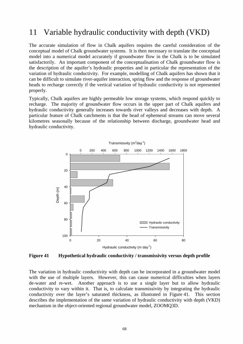
68
11 Variable hydraulic conductivity with depth (VKD) The accurate simulation of flow in Chalk aquifers requires the careful consideration of the conceptual model of Chalk groundwater systems. It is then necessary to translate the conceptual model into a numerical model accurately if groundwater flow in the Chalk is to be simulated satisfactorily. An important component of the conceptualisation of Chalk groundwater flow is the description of the aquifer’s hydraulic properties and in particular the representation of the variation of hydraulic conductivity. For example, modelling of Chalk aquifers has shown that it can be difficult to simulate river-aquifer interaction, spring flow and the response of groundwater heads to recharge correctly if the vertical variation of hydraulic conductivity is not represented properly.
Typically, Chalk aquifers are highly permeable low storage systems, which respond quickly to recharge. The majority of groundwater flow occurs in the upper part of Chalk aquifers and hydraulic conductivity generally increases towards river valleys and decreases with depth. A particular feature of Chalk catchments is that the head of ephemeral streams can move several kilometres seasonally because of the relationship between discharge, groundwater head and hydraulic conductivity.
Hydraulic conductivity (m day-1)
0 20 40 60 80
Dep
th (m
)
0
20
40
60
80
100
Transmissvity (m2day-1)
0 200 400 600 800 1000 1200 1400 1600 1800
Hydraulic conductivityTransmissivity
Figure 41 Hypothetical hydraulic conductivity / transmissivity versus depth profile
The variation in hydraulic conductivity with depth can be incorporated in a groundwater model with the use of multiple layers. However, this can cause numerical difficulties when layers de-water and re-wet. Another approach is to use a single layer but to allow hydraulic conductivity to vary within it. That is, to calculate transmissivity by integrating the hydraulic conductivity over the layer’s saturated thickness, as illustrated in Figure 41. This section describes the implementation of the same variation of hydraulic conductivity with depth (VKD) mechanism in the object-oriented regional groundwater model, ZOOMQ3D.

69
11.1 IMPLEMENTATION OF VKD IN ZOOMQ3D The implementation of VKD in ZOOMQ3D is based on two principal concepts. These are the definition of VKD profiles and VKD schemes. These two terms are used to describe both the incorporation of the mechanism in the model code and the input of data to the model.
11.1.1 VKD profiles A VKD profile describes the change in hydraulic conductivity with depth at a particular point in the aquifer. An example VKD profile is shown in Figure 42. Currently, VKD profiles represent the variation in hydraulic conductivity with elevation using a relatively simple method. Profiles are defined by two sections. In the lower section, between BOTTOMZ and PZ in Figure 42, hydraulic conductivity is constant. In the upper section, between PZ and TOPZ , hydraulic conductivity increases linearly with elevation. Because different values of hydraulic conductivity can be specified in the two orthogonal horizontal directions (x and y), six values are required to parameterise an individual profile:
1. The elevation of the base of the profile, BOTTOMZ .
2. The elevation of the top of the profile, TOPZ .
3. The elevation of the point of inflection, PZ .
4. The hydraulic conductivity in the x direction, *xK , below PZ .
5. The hydraulic conductivity in the y direction, *yK , below PZ .
6. The gradient of the profile above PZ , VKDGrad. This is equal to the increase in hydraulic conductivity per metre rise in elevation.
The value of the VKDGrad parameter may be either negative, zero or positive. Consequently, in addition to an increase in hydraulic conductivity with depth above PZ , hydraulic conductivity can be specified to decrease or remain constant. VKDGrad is given by
dZdK
dZdKVKDGrad yx ==
To calculate transmissivity the following equations are used
( ) ( )2PBOTTOM
*xx ZhVKDGrad5.0ZhKT −⋅+−=
( ) ( )2PBOTTOM
*yy ZhVKDGrad5.0ZhKT −⋅+−=
for PZh > , and,
( )BOTTOM*xx ZhKT −=
( )BOTTOM*yy ZhKT −=
for PZh ≤ , where h is the water table elevation.

70
groundwater head, h
ZP
ZBOTTOM
ZTOP
Slope -
VKDGrad
Hydraulic conductivity,
T = K ( h - BOTTOMZ
+ 0.5 VKDGrad ( h - ZP )2
)
K x
x x
K x
*
*
Figure 42 Parameters used to define VKD profiles in ZOOMQ3D
11.1.2 VKD schemes A VKD scheme defines the number of VKD profiles in the vertical, at a horizontal point, and the number of model layers that each profile in the scheme crosses. That is, a scheme simply stores how VKD profiles are arranged in the vertical at a horizontal nodal location. VKD profiles can be specified in any layer and at both unconfined and convertible nodes. The following points describe the use of VKD schemes.
1. A VKD scheme defines the number of VKD profiles in the vertical at a horizontal nodal location.
2. The number of VKD profiles in a scheme must be in the range zero to the number of numerical layers in the model.
3. Within a scheme, a single VKD profile can be defined to cross/represent only one or more than one model layers. The scheme defines which layers each VKD profile represents.
4. VKD profiles can be defined to cross layers of confined nodes. The confined nodes are not connected to the VKD profile and do not calculate their transmissivity by interrogating the profile.
5. A different scheme can be defined at each horizontal nodal location of the model.
6. The same scheme can be applied at multiple horizontal nodal locations.
Figure 43 shows a number of examples of different VKD schemes in a model with four layers. Consequently, the maximum number of profiles in the vertical is four. These examples are not intended to be physically realistic but rather meant to illustrate the flexibility of the method. This level of flexibility has been included with regard to the possible future development of the method. It may be the case that more complex but realistic variations of hydraulic conductivity with depth are defined at a later stage of model development. The model can easily be modified to incorporate such VKD profiles.

71
2
1
4
3
2
1
4
3
2
1
4
3
2
1
4
3
2
1
4
3
2
1
4
3
2
1
LayerNumber
LayerNumber
LayerNumber
LayerNumber
LayerNumber
LayerNumber
LayerNumber
LayerNumber 1 profile 4 profiles 2 profiles 2 profiles
0 profiles1 profile2 profiles 2 profiles
Scheme 1 Scheme 2 Scheme 3 Scheme 4
Scheme 8Scheme 7Scheme 6Scheme 5
ProfileLevel
ProfileLevel
ProfileLevel
ProfileLevel
ProfileLevel
ProfileLevel
ProfileLevel
ProfileLevel
1
1
11
1
1
1
2
22
22
3
4
1
2
3
4 4
3
Figure 43 Specification of VKD schemes in ZOOMQ3D

72
11.2 VKD INPUT FILES
11.2.1 VKD scheme data files
Input data to the model can be separated into two categories. First information must be read to define the number and types of schemes in the model. Second, data must be entered to define the VKD profiles at each horizontal nodal location of the model mesh. Two text input files are required to enter VKD scheme information into the model: ‘vkd.cod’ and ‘vkd.map’. The first of these ASCII text files, ‘vkd.cod’ contains the following lines of data:
NS 1NP 1
TOPI 1BOTI 2
TOPI 2BOTI …………… 1NP
TOPI 1NPBOTI
2NP 1TOPI 1
BOTI 2TOPI 2
BOTI …………… 2NPTOPI 2NP
BOTI
M M M M M M M
NSNP 1TOPI 1
BOTI 2TOPI 2
BOTI …………… NSNPTOPI NSNP
BOTI where
NS is the number of schemes in the model. iNP is the number of profiles in the ith scheme (i = 1 to NS).
jTOPI is the number of the top layer in the jth profile in the scheme (j = 1 to iNP ). jBOTI is the number of the bottom layer in the jth profile in the scheme (j = 1 to iNP ).
Therefore to define the eight schemes shown in Figure 43 ‘vkd.cod’ would contain the following lines of data
8 1 1 4 4 1 1 2 2 3 3 4 4 2 1 3 4 4 2 1 2 3 4 2 1 1 4 4 1 3 4 2 2 2 4 4 0
Once the configurations of the profiles within each scheme have been defined, information relating to the distribution of the schemes in the horizontal must be entered. This is performed using the text file ‘vkd.map’, which contains a map of the model mesh. The format of the file is the same as that of the map files described in Section 7.3. For example consider the file shown in Figure 44, which represents the square mesh that is also shown in the figure. At each node of the mesh a character is specified. Each letter of the alphabet corresponds to a VKD scheme defined in ‘vkd.cod’. Fifty-two letters, and therefore schemes, are allowed which are specified in the order a-z and then A-Z. Letter ‘a’ corresponds to the first scheme, ‘b’ to the second and ‘z’ to the twenty-sixth scheme. Letter ‘A’ corresponds to the twenty-seventh scheme, ‘B’ to the twenty-eighth and ‘Z’ to the fifty-second scheme. Figure 44 shows an example of a map file, which is used to distribute the VKD schemes defined in Figure 43 over the model domain. VKD profiles are not created at the horizontal nodal locations where an appropriate letter is not specified i.e. in this example where the character is not in the range ‘a’ to ‘h’. At these points horizontal conductivity is uniform in

73
the vertical direction within each layer. Again this example is not intended to be physically realistic but rather is used to illustrate the flexibility of the method.
a) Map of VKD schemes -----abbbcc ----abbccdd ---abccdddd --abccddeee --abcdddeef -abcddeefff abcddeeffgg bcddeeffggh cddeeffghhh cddeeffghhh cdeefgghhhh
b)
Figure 44 Example a) VKD scheme map file and b) associated model grid
11.2.2 VKD profile data files After defining which VKD scheme applies at each horizontal nodal location, values have to be read to parameterise each VKD profile in each scheme. At horizontal nodal locations represented by the letter ‘a’, in this example, data for only one profile is required. But at nodal locations represented by the letter ‘b’ data for four profiles must be read in. Four types of information are required for each VKD profile:
1. The hydraulic conductivity in the x direction, *xK , below PZ .
2. The hydraulic conductivity in the y direction, *yK , below PZ .
3. The gradient of the profile, VKDGrad, above PZ .
4. The elevation of the point of inflection, PZ .
VKD profile data must be entered into the model using either:
1. a pair of map and code files for each profile level for each VKD parameter or,
2. a numeric data file for each profile level for each VKD parameter.
As shown in Figure 43, profiles can be on the same level but represent/cross different model layers. Reiterating, VKD profile data is input for each profile level and not for each model layer.
For the example shown in Figure 43, either four pairs of map and codes or four numeric data files are required for each of the four VKD parameters: *
xK , *yK , VKDGrad, PZ . This is
because the maximum number of profiles in the vertical is four. An example set of map and code files is shown in Figure 45a for the first profile level and an example set of numeric data files is shown in Figure 45b.
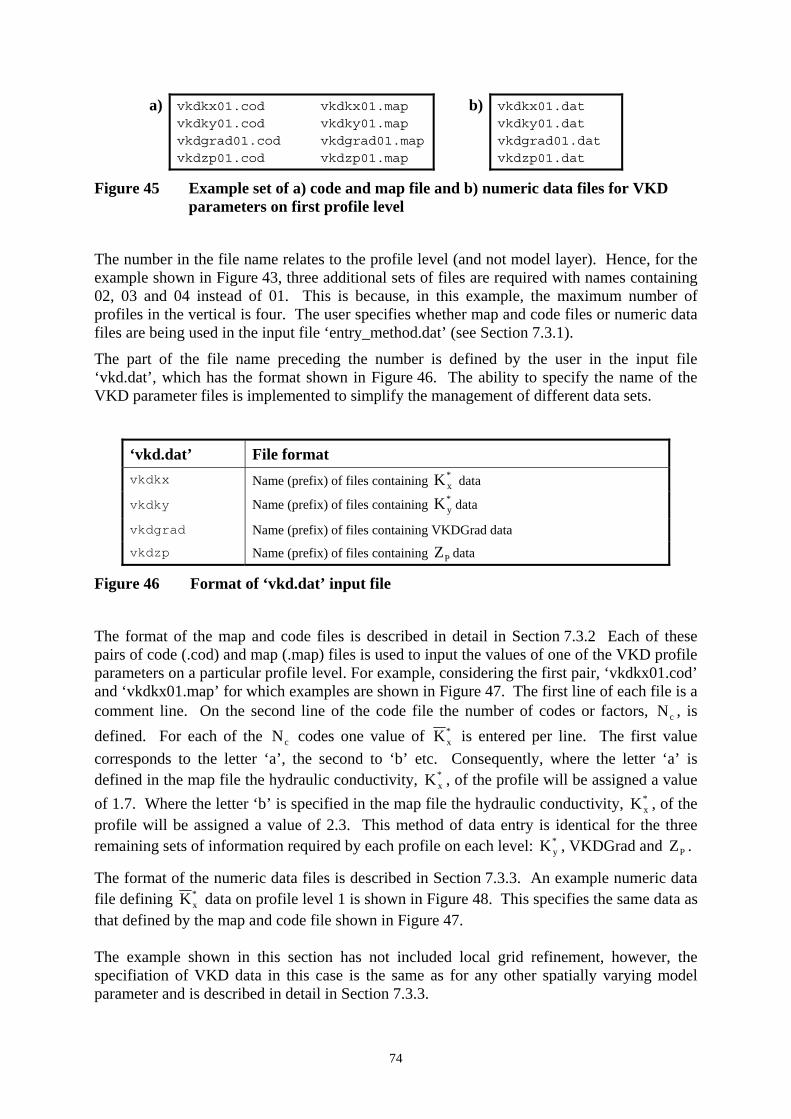
74
a) vkdkx01.cod vkdkx01.map vkdky01.cod vkdky01.map vkdgrad01.cod vkdgrad01.map vkdzp01.cod vkdzp01.map
b) vkdkx01.dat vkdky01.dat vkdgrad01.dat vkdzp01.dat
Figure 45 Example set of a) code and map file and b) numeric data files for VKD parameters on first profile level
The number in the file name relates to the profile level (and not model layer). Hence, for the example shown in Figure 43, three additional sets of files are required with names containing 02, 03 and 04 instead of 01. This is because, in this example, the maximum number of profiles in the vertical is four. The user specifies whether map and code files or numeric data files are being used in the input file ‘entry_method.dat’ (see Section 7.3.1).
The part of the file name preceding the number is defined by the user in the input file ‘vkd.dat’, which has the format shown in Figure 46. The ability to specify the name of the VKD parameter files is implemented to simplify the management of different data sets.
‘vkd.dat’ File format vkdkx Name (prefix) of files containing *
xK data
vkdky Name (prefix) of files containing *yK data
vkdgrad Name (prefix) of files containing VKDGrad data
vkdzp Name (prefix) of files containing PZ data
Figure 46 Format of ‘vkd.dat’ input file
The format of the map and code files is described in detail in Section 7.3.2 Each of these pairs of code (.cod) and map (.map) files is used to input the values of one of the VKD profile parameters on a particular profile level. For example, considering the first pair, ‘vkdkx01.cod’ and ‘vkdkx01.map’ for which examples are shown in Figure 47. The first line of each file is a comment line. On the second line of the code file the number of codes or factors, cN , is defined. For each of the cN codes one value of *
xK is entered per line. The first value corresponds to the letter ‘a’, the second to ‘b’ etc. Consequently, where the letter ‘a’ is defined in the map file the hydraulic conductivity, *
xK , of the profile will be assigned a value of 1.7. Where the letter ‘b’ is specified in the map file the hydraulic conductivity, *
xK , of the profile will be assigned a value of 2.3. This method of data entry is identical for the three remaining sets of information required by each profile on each level: *
yK , VKDGrad and PZ .
The format of the numeric data files is described in Section 7.3.3. An example numeric data file defining *
xK data on profile level 1 is shown in Figure 48. This specifies the same data as that defined by the map and code file shown in Figure 47. The example shown in this section has not included local grid refinement, however, the specifiation of VKD data in this case is the same as for any other spatially varying model parameter and is described in detail in Section 7.3.3.

75
Code file Map file
VKDKx code data 2 1.7 2.3
Map for VKDKx parameter on profile level 1 -----aaaaaa ----aaaaaaa ---aaaaaabb --aaaaaabbb --aaaaaabbb -aaaaabbbbb aaaaabbbbbb aaaabbbbbbb aaabbbbbbbb aaabbbbbbbb aabbbbbbbbb
Figure 47 Example code file ‘vkdkx01.cod’ and map file ‘vkdkx01.map’
Numeric data for VKDKx parameter on profile level 1 -999 -999 -999 -999 -999 1.7 1.7 1.7 1.7 1.7 1.7 -999 -999 -999 -999 1.7 1.7 1.7 1.7 1.7 1.7 1.7 -999 -999 -999 1.7 1.7 1.7 1.7 1.7 1.7 2.3 2.3 -999 -999 1.7 1.7 1.7 1.7 1.7 1.7 2.3 2.3 2.3 -999 -999 1.7 1.7 1.7 1.7 1.7 1.7 2.3 2.3 2.3 -999 1.7 1.7 1.7 1.7 1.7 2.3 2.3 2.3 2.3 2.3 1.7 1.7 1.7 1.7 1.7 2.3 2.3 2.3 2.3 2.3 2.3 1.7 1.7 1.7 1.7 2.3 2.3 2.3 2.3 2.3 2.3 2.3 1.7 1.7 1.7 2.3 2.3 2.3 2.3 2.3 2.3 2.3 2.3 1.7 1.7 1.7 2.3 2.3 2.3 2.3 2.3 2.3 2.3 2.3 1.7 1.7 2.3 2.3 2.3 2.3 2.3 2.3 2.3 2.3 2.3
Figure 48 Example numeric data file ‘vkdkx01.dat’

76
12 The solution process 12.1 SUCCESSIVE OVER-RELAXATION SOLUTION METHOD The point successive over-relaxation (SOR) method is the only numerical solution technique currently implemented in ZOOMQ3D. SOR is implemented first because it is easy to apply, and thus modify, and because it is generally robust. In some models the matrix of coefficients of the finite difference equations is modified during the solution of a time-step, for example by updating transmissivity as groundwater head changes when simulating unconfined aquifers. This process is not allowed within ZOOMQ3D and the matrix of coefficients remains fixed during the solution of a time-step. This eliminates some potential problems of convergence when using SOR.
The SOR solver in ZOOMQ3D scans each grid of the model mesh. It begins by updating the solution on the base grid and then repeatedly steps down the grid hierarchy to the next finest grid level. One SOR iteration is performed at each node on each grid, within each grid level, before moving to the next finest grid level. After each of the grids has been scan the process returns to the base grid. The solver converges after a number of scans across all the grids when the maximum nodal flow imbalance falls below a user-defined value. The simulation then progresses to the next time-step.
The name of the file used to enter information relating to the solution method is specified by the user in the input file ‘zoomq3d.dat’. The format of the input file, for example named ‘sor.dat’, is shown in Figure 49 where
iSolve is an integer flag indicating which solution method is being used.
SOR is the only solution method currently implemented in ZOOMQ3D and thus only a 1 can be entered on this line.
ω is the successive over-relaxation factor (ω). 0.20.1 <ω≤ . CCrit is the convergence criterion as a maximum permissible nodal flow
imbalance (m3 day-1). MaxIter is the maximum number of iterations per time-step. MaxTChange is the maximum permissible change in transmissivity (m2 day-1) over
a cycle (see Section 7.2.2). MaxCycles is the maximum number of cycles (see Section 7.2.2). CheckIter is the number of iterations after which to check for convergence. WriteIter is the number of iterations after which to output information on the
progress of the solution process to ‘zoomq3d.out’.
An example file, ‘sor.dat’, is shown in Figure 50.
iSolve ω CCrit MaxIter MaxTChange MaxCycles CheckIter WriteIter
Figure 49 Format of SOR numerical solver input file

77
1 1.7 1.0 5000 1.0 5 10 500
Figure 50 Example ‘sor.dat’ file

78
13 Activating / de-activating nodes 13.1 DE-WATERING AND RE-WETTING Model nodes de-water when the groundwater head falls below their base. When this occurs the node is made inactive and is removed from the matrix of finite difference equations. A mechanism is implemented to re-wet nodes when groundwater levels rise again. The mechanism is based on the examination of the groundwater head at the neighbouring nodes of the inactive node. Two options are defined. Either the horizontally adjacent nodes can be examined or the node in the layer beneath can be interrogated to determine if the de-watered node should be reactivated.
Three parameters are defined to allow the re-wetting of nodes, each of which is described in the following three sub-sections. These parameters are
1. a wetting flag,
2. a wetting threshold and,
3. a post wetting head value.
13.1.1 Wetting flag The wetting flag is a character variable which is either an ‘h’ or a ‘v’. If it is an ‘h’ (horizontal) then the inactive node’s neighbours on the same layer are examined to determine if their head has risen above the wetting threshold. If it is a ‘v’ (vertical) then the inactive node’s neighbour in the layer below is examined to determine if its head has risen above the wetting threshold. In the bottom model layer, only an ‘h’ can be defined. Each node in the model must be assigned a wetting flag. This is performed using the following inputs files.
Input file names and format The wetting flag is defined using a map file with the name ‘wetflag##.map’ for each model layer.
The ## symbols must be replaced by a two digit (01 to 99) number representing the layer to which the data files refer. The upper layer is layer 01 and their numbers are incremented from the top to the bottom of the model. The format of map files is described in Section 7.3. An example wetting flag map file is shown in Figure 51.
---- Map for grid on level: 1 Bottom left: 0,0 Top right: 10000,10000 ---- hhhhhhhhhhh hhhhhhhhhhh hhhhhhhhhhh hhhhhhhhhhh hhhhhhhhhhh hhhhhhhhhhh hhhhhhhhhhh hhhhhhhhhhh hhhhhhhhhhh hhhhhhhhhhh hhhhhhhhhhh
Figure 51 Example ‘wetflag##.map’ file
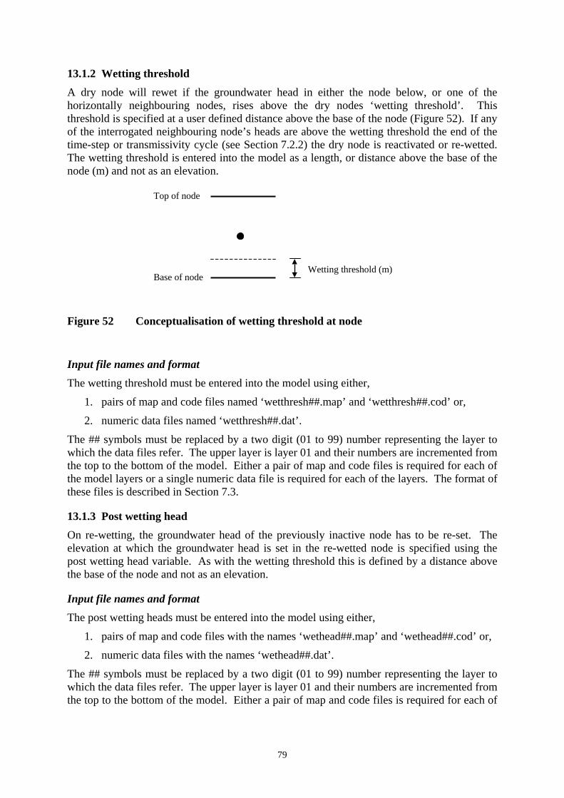
79
13.1.2 Wetting threshold A dry node will rewet if the groundwater head in either the node below, or one of the horizontally neighbouring nodes, rises above the dry nodes ‘wetting threshold’. This threshold is specified at a user defined distance above the base of the node (Figure 52). If any of the interrogated neighbouring node’s heads are above the wetting threshold the end of the time-step or transmissivity cycle (see Section 7.2.2) the dry node is reactivated or re-wetted. The wetting threshold is entered into the model as a length, or distance above the base of the node (m) and not as an elevation.
Figure 52 Conceptualisation of wetting threshold at node
Input file names and format
The wetting threshold must be entered into the model using either,
1. pairs of map and code files named ‘wetthresh##.map’ and ‘wetthresh##.cod’ or,
2. numeric data files named ‘wetthresh##.dat’.
The ## symbols must be replaced by a two digit (01 to 99) number representing the layer to which the data files refer. The upper layer is layer 01 and their numbers are incremented from the top to the bottom of the model. Either a pair of map and code files is required for each of the model layers or a single numeric data file is required for each of the layers. The format of these files is described in Section 7.3.
13.1.3 Post wetting head
On re-wetting, the groundwater head of the previously inactive node has to be re-set. The elevation at which the groundwater head is set in the re-wetted node is specified using the post wetting head variable. As with the wetting threshold this is defined by a distance above the base of the node and not as an elevation.
Input file names and format The post wetting heads must be entered into the model using either,
1. pairs of map and code files with the names ‘wethead##.map’ and ‘wethead##.cod’ or,
2. numeric data files with the names ‘wethead##.dat’.
The ## symbols must be replaced by a two digit (01 to 99) number representing the layer to which the data files refer. The upper layer is layer 01 and their numbers are incremented from the top to the bottom of the model. Either a pair of map and code files is required for each of
Top of node
Base of node Wetting threshold (m)
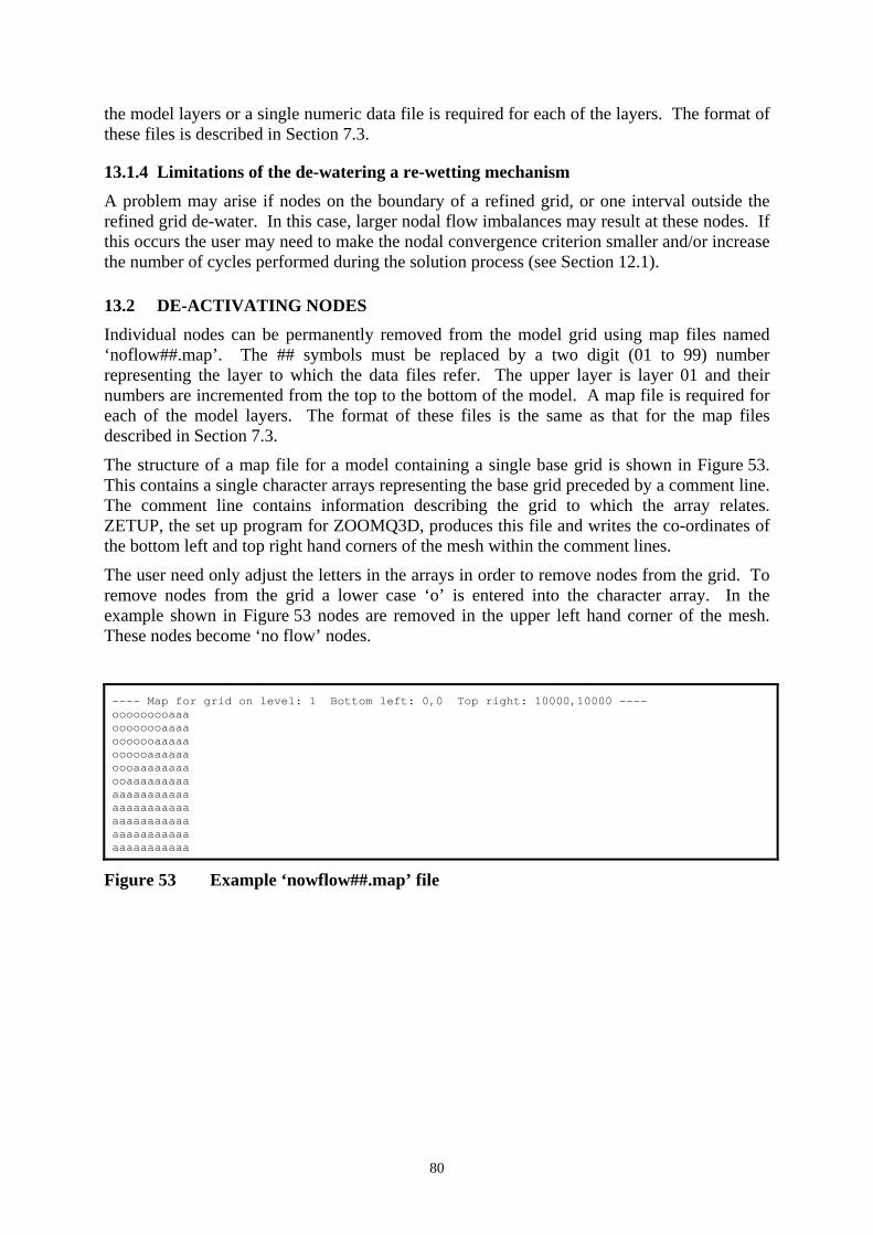
80
the model layers or a single numeric data file is required for each of the layers. The format of these files is described in Section 7.3.
13.1.4 Limitations of the de-watering a re-wetting mechanism A problem may arise if nodes on the boundary of a refined grid, or one interval outside the refined grid de-water. In this case, larger nodal flow imbalances may result at these nodes. If this occurs the user may need to make the nodal convergence criterion smaller and/or increase the number of cycles performed during the solution process (see Section 12.1).
13.2 DE-ACTIVATING NODES Individual nodes can be permanently removed from the model grid using map files named ‘noflow##.map’. The ## symbols must be replaced by a two digit (01 to 99) number representing the layer to which the data files refer. The upper layer is layer 01 and their numbers are incremented from the top to the bottom of the model. A map file is required for each of the model layers. The format of these files is the same as that for the map files described in Section 7.3.
The structure of a map file for a model containing a single base grid is shown in Figure 53. This contains a single character arrays representing the base grid preceded by a comment line. The comment line contains information describing the grid to which the array relates. ZETUP, the set up program for ZOOMQ3D, produces this file and writes the co-ordinates of the bottom left and top right hand corners of the mesh within the comment lines.
The user need only adjust the letters in the arrays in order to remove nodes from the grid. To remove nodes from the grid a lower case ‘o’ is entered into the character array. In the example shown in Figure 53 nodes are removed in the upper left hand corner of the mesh. These nodes become ‘no flow’ nodes.
---- Map for grid on level: 1 Bottom left: 0,0 Top right: 10000,10000 ---- ooooooooaaa oooooooaaaa ooooooaaaaa oooooaaaaaa oooaaaaaaaa ooaaaaaaaaa aaaaaaaaaaa aaaaaaaaaaa aaaaaaaaaaa aaaaaaaaaaa aaaaaaaaaaa
Figure 53 Example ‘nowflow##.map’ file
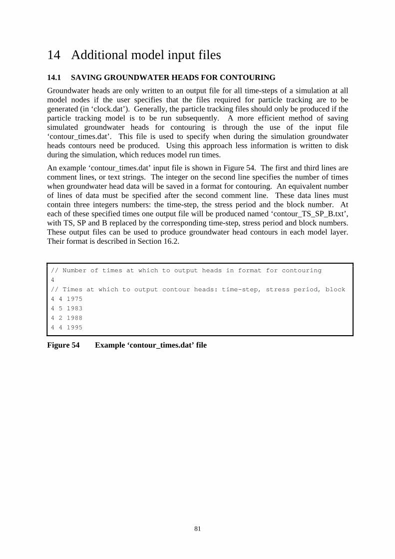
81
14 Additional model input files 14.1 SAVING GROUNDWATER HEADS FOR CONTOURING Groundwater heads are only written to an output file for all time-steps of a simulation at all model nodes if the user specifies that the files required for particle tracking are to be generated (in ‘clock.dat’). Generally, the particle tracking files should only be produced if the particle tracking model is to be run subsequently. A more efficient method of saving simulated groundwater heads for contouring is through the use of the input file ‘contour_times.dat’. This file is used to specify when during the simulation groundwater heads contours need be produced. Using this approach less information is written to disk during the simulation, which reduces model run times.
An example ‘contour_times.dat’ input file is shown in Figure 54. The first and third lines are comment lines, or text strings. The integer on the second line specifies the number of times when groundwater head data will be saved in a format for contouring. An equivalent number of lines of data must be specified after the second comment line. These data lines must contain three integers numbers: the time-step, the stress period and the block number. At each of these specified times one output file will be produced named ‘contour_TS_SP_B.txt’, with TS, SP and B replaced by the corresponding time-step, stress period and block numbers. These output files can be used to produce groundwater head contours in each model layer. Their format is described in Section 16.2.
// Number of times at which to output heads in format for contouring 4 // Times at which to output contour heads: time-step, stress period, block 4 4 1975 4 5 1983 4 2 1988 4 4 1995
Figure 54 Example ‘contour_times.dat’ file

82
14.2 SELECTING WHICH DATA INPUT FILES TO USE The names of many of the ZOOMQ3D input files are fixed and invariable. However, some file names can be specified by the user in the input file ‘zoomq3d.dat’. These files are distinguished in Table 6. ZOOMQ3D reads the file names and opens the corresponding input data files. Consequently, it is easy to modify a model by using an input file that contains the same type of data but which has a different name. The format of the file ‘zoomq3d.dat’ is shown in Table 6. It must contain eighteen text strings, representing the input file names, in the order shown in the figure. These names are those of the example set of files, which are used throughout this manual.
Even though some of the model features may not be included in a model, and consequently some of their related input and output files not opened, all eighteen file names must be listed in ‘zoomq3d.dat’.
Table 6 Format of ‘zoomq3d.dat’ input file
Description of named file (not part of the file) sor.dat Numerical solver input file fixedheads.dat Input file specifying fixed heads inside the model boundary initialh.dat Input file containing initial groundwater head for the whole model obswells.dat Input file containing observation well data obswells.out Output file storing groundwater head hydrographs at obs wells pumping.dat Input file containing abstraction well data recharge.dat Main recharge data input file gauging_stations.dat Input file containing river baseflow monitoring point data gauging_stations.out Output file in which river baseflow hydrographs are stored riverflow.out Output file in which river baseflow at specific times are stored accretion.out Output file in which river flow accretion profile data is stored initialflow.dat Input specifying initial river baseflows river_inputs.dat Input file specifying time-variant discharges to rivers obsleak.dat Input file specifying which leakage nodes to monitor obsleak.out Output file storing flows to/from leakage nodes over time finalh.out Output file in which final groundwater head profile is stored contour.txt Output file to which head data is written for contouring flowbal.out Output file to which nodal flow balance information is written
83
PART 3 – Model output
15 Summary of output files produced by ZOOMQ3D 15.1 THE PHILOSOPHY OF MODEL OUPUT The philosophy behind the structure of ZOOMQ3D model output is to separate different types of data between files. That is, each file contains one specific type of information only. This simplifies the post-processing of model output and means that standard software packages can be used to interpret and visualise results. All the output files have a very simple format and are easily examined using a text editor or processed using spreadsheet software.
The list of output files produced by ZOOMQ3D is presented in Table 7. Though there are eighteen files listed, not all of these are always produced. For example, if no rivers are included the model, three fewer files are created. Each of the ZOOMQ3D output files is described in the following section. All output files containing columns of data are space separated.
Table 7 List of all ZOOMQ3D output files Model feature Relevant file names Relevant
section Groundwater heads
1. Over time 2. For restarting model 3. For contouring
obswells.out finalh.out contour.txt, contour_##_##_####.txt
16.1 16.3 16.2
Boundary conditions 1. Head-dependent leakage
nodes 2. Springs
obsleak.out springs.out
16.10
16.11
Rivers gauging_stations.out, accretion.out, riverflow.out 16.4-16.6 Water balances
1. Global water balances 2. Nodal flow balances
global.out, global_tv.out flowbal.out
16.9 16.8
De-watering and re-wetting dewatering.out 16.7 Multi-aquifer wells multi_wells.out 16.12 Progress of solution zoomq3d.out, transcycle.out 16.13-16.14 Output for particle tracking heads.txt, flowbal.txt 16.15
15.2 PROCESSING MODEL OUTPUT Model output is readily processed and visualised using spreadsheet software, Surfer (Golden Software Inc., 1994) and a text editor. Because each model file contains only one type of data, the user is not required to extract information from many different locations within a single file. All text files are space delimited.

84
16 Description of output file formats The format of each of the files listed in Table 7 is described in detail in the following sub-sections.
16.1 OBSERVATION WELL DATA The nodes at which groundwater head is monitored over time are specified in the input file named in the file ‘zoomq3d.dat’, for example ‘obswells.dat’. The time versus groundwater head record at these nodes is output to the file also named in ‘zoomq3d.dat’, for example ‘obswells.out’. This output file contains one line of data for each time-step of the simulation with the following format day stress_period block MJD_time time_elapsed h1 h2 h3 h4 … hn
where
day is the end of the day when the flow was recorded,
stress period is the stress period number,
block is the time block number of the flow measurement,
MJD_time is the time simulated from the start time in Modified Julian day format,
time_elapsed is the time simulated since the beginning of the model run (days),
h1 is the head (m) in the first observation well defined in ‘obswells.dat’,
h2 is the head (m) in the second observation well defined in ‘obswells.dat’,
hn is the head (m) in the nth observation well defined in ‘obswell.dat’.
The output file is space delimited and is easily opened using spreadsheet software, which can be used to produce groundwater head hydrographs.
16.2 CONTOURING GROUNDWATER HEADS The computed groundwater heads are written to an output file in a format suitable for contouring. The name of the output file is specified in the input file ‘zoomq3d.dat’. This output file, for example ‘contour.txt’ contains groundwater head data for a single time-step only and is over-written periodically during the simulation. The frequency with which the file is produced is defined in the input file ‘clock.dat’. It is created after either every, time-step, stress period or block, or only for the final time-step in the simulation. Each time it is written, the previous data set is lost. However, groundwater head data, in this format, can be saved by specifying the times of interest in the input file ‘contour_times.dat’ (see Section 14.1).
The format of this output file is simple and is suitable for contouring using Surfer (Golden Software Inc., 1994). The groundwater head at each horizontal location is written on a separate line. The file has the following format x y h1 h2 h3 … hn
where
x is the x co-ordinate of the grid point,
y is the y co-ordinate of the grid point,
hi is the groundwater head in the ith layer.
85
If a node is dry the groundwater head value is replaced by –999.
ZETUP produces a Surfer (Golden Software Inc., 1994) blanking file, which can be used to blank the data around the boundary of the model when contouring. This file is called ‘boundary.bln’.
16.3 GROUNDWATER HEADS IN FORMAT TO RE-START A SIMULATION Groundwater heads are written to an output file in a format that enables a model run to be re-started from conditions modelled during the current simulation. The name of this output file, for example ‘finalh.out’, is specified in the input file ‘zoomq3d.dat’. It contains the groundwater head at each node of the model at the end of a single time-step and is over-written periodically during the simulation. The frequency with which the file is produced is defined in ‘clock.dat’. It is created after either every, time-step, stress period or block, or only for the final time-step in the simulation. Each time it is written, the previous data set is lost.
The file has exactly the same format as the input file described in Section 8.2, which is used to define initial conditions for a model. Consequently, in order to use this output file to re-start a simulation it is only necessary to rename it appropriately.
16.4 RIVER FLOW GAUGING The river nodes at which the baseflow is monitored over time are specified in the input file named in the file ‘zoomq3d.dat’, for example ‘gauging_stations.dat’. The time-discharge record at these nodes is output to the file also named in ‘zoomq3d.dat’, for example ‘gauging_stations.out’. This output file contains one line of data for each time-step of the simulation with the following format day stress_period block MJD_time time_elapsed Q1 Q2 Q3 Q4 … Qn
where
day is the end of the day when the flow was recorded,
stress period is the stress period number,
block is the time block number of the flow measurement,
MJD_time is the time simulated from the start time in Modified Julian day format,
time_elapsed is the time simulated since the beginning of the model run (days),
Q1 is the flow (m3 day-1) in the first river node defined in ‘gauging_stations.dat’,
Q2 is the flow (m3 day-1) in the second river node defined in ‘gauging_stations.dat’,
Qn is the flow (m3 day-1) in the nth river node defined in ‘gauging_stations.dat’.
The river nodes are listed in the same order as they are defined in the input file. The output file is space delimited and is easily opened using spreadsheet software, which can be used to produce river baseflow hydrographs.
16.5 RIVER BASEFLOW ACCRETION PROFILES River flow accretion data is written to the output file named in ‘zoomq3d.dat’, for example ‘accretion.out’. The data is in a form suitable for the rapid production of accretion profiles using spreadsheet software. This output file contains flow data for a single time-step only and is over-written periodically during the simulation. The frequency with which the file is produced is defined in the input file ‘clock.dat’. It is created after either every, time-step,

86
stress period or block, or only for the final time-step in the simulation. Each time it is written, the previous data set is lost. Accretion profiles at different times can be saved by specifying each node along the river section of interest as a gauging station in the relevant input file (see Section 9.5.5).
The output file is space delimited and has a simple format. An example output file is shown in Figure 55. The number of rivers in the model is written on the first line. A block of data then follows for each river. Eleven columns of data are defined within each block, which are separated by comment lines composed of a series of dashes. Each row represents one node of the river. The eleven columns contain the following data
1. River branch number.
2. River node number.
3. x co-ordinate of river node (m).
4. y co-ordinate of river node (m).
5. Distance downstream from uppermost node in branch (m).
6. Baseflow (m3day-1).
7. Groundwater head (m).
8. River stage (m).
9. River bed elevation (m).
10. River bed vertical hydraulic conductivity under effluent conditions (m day-1).
11. River bed vertical hydraulic conductivity under influent conditions (m day-1).
16.6 RIVER BASEFLOWS IN A FORMAT TO RE-START A SIMULATION River baseflows are written to an output file in a format that enables a model run to be re-started from conditions modelled during the current simulation. The name of this output file, for example ‘riverflow.out’, is specified in the input file ‘zoomq3d.dat’. It contains the river baseflow at each node each river in the model at the end of a single time-step and is over-written periodically during the simulation. The frequency with which the file is produced is defined in ‘clock.dat’. It is created after either every, time-step, stress period or block, or only for the final time-step in the simulation. Each time it is written, the previous data set is lost.
The file has exactly the same format as the input file described in Section 9.5.3, which is used to define initial river baseflow conditions. Consequently, in order to use this output file to re-start a simulation it is only necessary to rename it appropriately.

87
2
----------------------
River 1
Branch Node X Y Dist.downstream Flow Head Stage Bed Elevation Kz Effluent Kz Influent
1 9 294500 572500 0 5765.87 7.80 7.5 6.5 1 1
1 8 295000 572500 500 5931.98 7.53 7.5 6.5 1 1
1 7 295500 572500 1000 7050.44 7.68 7.5 6.5 1 1
1 6 296000 572000 1707.11 7362.65 7.54 7.49 6.49 1 1
1 5 296000 571500 2207.11 8172.72 7.35 7.21 6.21 1 1
etc for each node in each branch of river 1
----------------------
River 2
Branch Node X Y Dist.downstream Flow Head Stage Bed Elevation Kz Effluent Kz Influent
1 14 292500 575500 0 12500 32.69 68 67 1 1
1 13 293000 575500 500 17239.4 16.42 16.03 15.03 1 1
1 12 293500 576000 1207.11 21484.3 8.85 8.55 7.55 1 1
1 11 294000 576500 1914.21 31937.7 7.09 7 6 1 1
1 10 294000 576000 2414.21 32773.8 8.08 8 7 1 1
1 9 294500 576000 2914.21 36011.6 6.36 6.09 5.09 1 1
etc for each node in branch 1 of river 1
2 20 292000 578000 0 2000 22.12 37 36 1 1
2 19 292500 578000 500 0 21.7 36 35 1 1
2 18 293000 578000 1000 0 17.13 33.53 32.53 1 1
etc for each node in branch 2 of river 1
Figure 55 Example output file containing river baseflow accretion data

88
16.7 DE-WATERING AND RE-WETTING At the end of each time-step information is written to the file ‘dewatering.out’ informing the user of which nodes have de-watered and which have re-wetted. The layer number and co-ordinate of each of these nodes is written to the file.
16.8 NODAL FLOW BALANCES Nodal flow balance information for every node in the model is written to the file, ‘flowbal.out’, for example, named in the input file ‘zoomq3d.dat’. This output file contains flow balance data for a single time-step only and is over-written periodically during the simulation. The frequency with which the file is produced is defined in the input file ‘clock.dat’. It is created after either every, time-step, stress period or block, or only for the final time-step in the simulation. It is always re-written at the end of the simulation. The first line of the file is a text string that specifies the time at which information is output. The second line contains the headings for the following columns of data. Each subsequent line represents one node in the model. A description of each column is given in Table 8. The file is space delimited and is readily opened using spreadsheet software for manipulation.
Table 8 Data contained in nodal flow balance output file
Column of file
Description of data (Rates of flow are for the last time-step only)
1 Layer of the node 2 x co-ordinate of the node 3 y co-ordinate of the node 4 Area of the node (m2) 5 Flow imbalance at the node (m3 day-1) 6 Inflow to the node in the x-direction from the left (m3 day-1) 7 Outflow from the node in the x-direction to the right (m3 day-1) 8 Inflow to the node in the y-direction from below (m3 day-1) 9 Outflow from the node in the y-direction to above (m3 day-1) 10 Inflow to the node in the z-direction through the base (m3 day-1) 11 Outflow from the node in the z-direction through the top (m3 day-1) 12 Specified inflow at the boundary (if a boundary node) (m3 day-1) 13 Rate of change of storage at node (m3 day-1). Positive values are increases in storage. 14 Recharge applied at the node (m3 day-1) 15 Rate of leakage between the aquifer and the river (m3 day-1)
Positive values represent influent river nodes 16 Rate of leakage to a leakage node (m3 day-1)
Positive values represent an outflow from the aquifer 17 Rate of abstraction at the node (m3 day-1)
Abstraction is represented by negative values 18 Spring flow (m3 day-1)
Positive values represent flow of the aquifer (negative values not possible)

89
16.9 GLOBAL FLOW BALANCES Global flow balance information for the model is written to the file ‘global.out’. This output file contains flow balance data for a single time-step only and is over-written periodically during the simulation. The frequency with which the file is produced is defined in the input file ‘clock.dat’. It is created after either every, time-step, stress period or block, or only for the final time-step in the simulation. It is always re-written at the end of the simulation. This file gives a water balance for the whole model over a time-step. An example file is shown in Figure 56. Information includes the total recharge to the model, the total flow across its boundary, the total abstraction, the total downstream flow and anthropogenic input to each river, the total outflow to leakage nodes and fixed heads, the total change in storage over the last time-step and the total spring flow. These flow rates are summed to give a global flow imbalance figure, which is written on the last line of the file.
GLOBAL FLOW BALANCE AT END OF 4/12/1974 (TS/SP/BLOCK) --------------------------------- Total recharge: 188750 m3/d Total boundary inflow: 0 m3/d Total abstraction: 32900 m3/d River 1 Downstream flow: 7421.12 m3/d Anthropogenic input: 5000 m3/d River 2 Downstream flow: 40684.7 m3/d Anthropogenic input: 32000 m3/d River 3 Downstream flow: 1.26626e+006 m3/d Anthropogenic input: 1.217e+006 m3/d River 4 Downstream flow: 63027.3 m3/d Anthropogenic input: 24000 m3/d Total leakage out of aquifer: 56443.4 m3/d Total outflow to fixed heads: 0 m3/d Total increase in aquifer storage: 7.17061e-012 m3/d TOTAL INFLOW: 1.46675e+006 m3/d TOTAL OUTFLOW: 1.46673e+006 m3/d GLOBAL FLOW IMBALANCE: 15.6715 m3/d 0.00106845 % of total inflow
Figure 56 Example global flow balance output file
16.9.1 Time-variant global flow balances Global flow balance information for every time-step of a simulation is written to the file, ‘global_tv.out’. The file contains the columns of data listed in Table 9. One line of data is written to the file per time-step. The file is space delimited and is readily opened using spreadsheet software for manipulation.

90
Table 9 Data contained in ‘global_tv.out’
Column Description of data
1 Time within stress period (days)
2 Stress period number
3 Block number
4 Time since start of simulation (days)
5 Total recharge (m3 day-1)
6 Total inflow at model boundary (m3 day-1)
7 Total abstraction (m3 day-1)
8 Total outflow from rivers (m3 day-1)
9 Total discharge/inflow to rivers (m3 day-1)
10 Total flow through leakage nodes (m3 day-1). Positive out of aquifer.
11 Total outflow to fixed head nodes (m3 day-1)
12 Total storage increase (m3 day-1). Positive values are increases in storage
13 Total spring flow (m3 day-1)
14 Global flow imbalance (m3 day-1)
16.10 MONITORING LEAKAGES The leakage nodes at which the flow is monitored over time are specified in the input file named in the file ‘zoomq3d.dat’, for example ‘obsleak.dat’. The time-discharge record at these nodes is output to the file also named in ‘zoomq3d.dat’, for example ‘obsleak.out’. This output file contains one line of data for each time-step of the simulation with the following format day stress_period block MJD_time time_elapsed Q1 Q2 Q3 Q4 … Qn
where
day is the end of the day when the flow was recorded,
stress period is the stress period number,
block is the time block number of the flow measurement,
MJD_time is the time simulated from the start time in Modified Julian day format,
time_elapsed is the time simulated since the beginning of the model run (days),
Q1 is the flow (m3 day-1) through the first leakage node defined in ‘obsleak.dat’,
Q2 is the flow (m3 day-1) through the second leakage node defined in ‘obsleak.dat’,
Qn is the flow (m3 day-1) through the nth leakage node defined in ‘obsleak.dat’.
The leakage nodes are listed in the same order as they are defined in the input file. The flow rates, Qi , are positive when flow is out of the aquifer and negative when flow is into the aquifer.
The output file is space delimited and is easily opened using spreadsheet software, which can be used to produce flow hydrographs.

91
16.11 SPRING FLOWS The time-discharge record at the springs included in the model is output to the file ‘springs.out’. This output file contains one line of data for each time-step of the simulation with the following format day stress_period block MJD_time time_elapsed Q1 Q2 Q3 Q4 … Qn
where
day is the end of the day when the flow was recorded,
stress period is the stress period number,
block is the time block number of the flow measurement,
MJD_time is the time simulated from the start time in Modified Julian day format,
time_elapsed is the time simulated since the beginning of the model run (days),
Q1 is the flow (m3 day-1) out of the first spring defined in ‘springs.dat’,
Q2 is the flow (m3 day-1) out of the second spring defined in ‘springs.dat’,
Qn is the flow (m3 day-1) out of the nth spring defined in ‘springs.dat’.
The spring flows are listed in the same order as they are defined in the input file. The output file is space delimited and is easily opened using spreadsheet software, which can be used to produce spring flow hydrographs.
16.12 MULTI-LAYER WELLS Flow and head data associated with multi-layer wells is output to the file ‘multi_wells.out’. This output file contains one line of data for each time-step of the simulation. It is a space separated column text file and contains columns of data in the following format day stress_period block MJD_time time_elapsed Qtotal Qi Hw hi
where
day is the end of the day when the flow was recorded,
stress period is the stress period number,
block is the time block number of the flow measurement,
MJD_time is the time simulated from the start time in Modified Julian day format,
time_elapsed is the time simulated since the beginning of the model run,
Qtotal is the pumping rate of the multi-layer well calculated by summing the flow into the well from each aquifer node,
Qi is the flow into the borehole from layer i,
Hw is the water level in the borehole,
hi is the head at the aquifer node in layer i.
There is one complete set of the columns Qtotal , Qi , Hw , hi for each multi-layer well in the model. Within each of set of these columns there are n columns of Qi and n columns of hi data, where n is the number of layers to which the multi-layer well is connected.
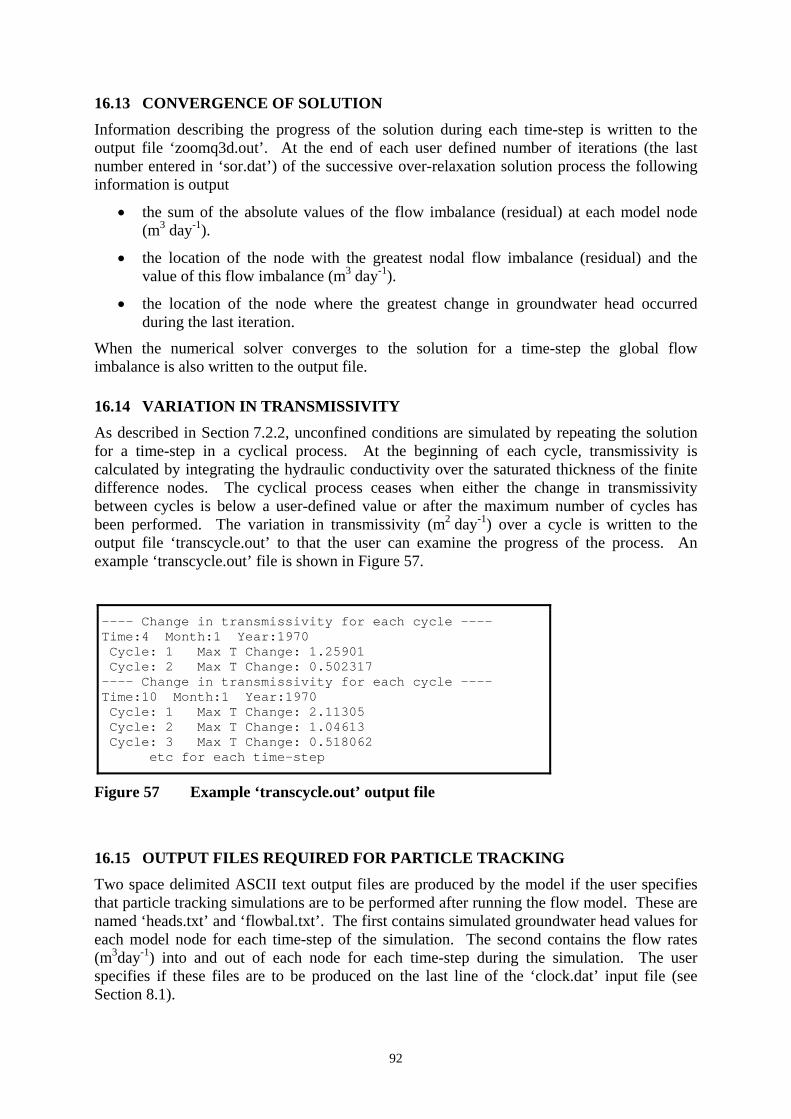
92
16.13 CONVERGENCE OF SOLUTION Information describing the progress of the solution during each time-step is written to the output file ‘zoomq3d.out’. At the end of each user defined number of iterations (the last number entered in ‘sor.dat’) of the successive over-relaxation solution process the following information is output
• the sum of the absolute values of the flow imbalance (residual) at each model node (m3 day-1).
• the location of the node with the greatest nodal flow imbalance (residual) and the value of this flow imbalance (m3 day-1).
• the location of the node where the greatest change in groundwater head occurred during the last iteration.
When the numerical solver converges to the solution for a time-step the global flow imbalance is also written to the output file.
16.14 VARIATION IN TRANSMISSIVITY As described in Section 7.2.2, unconfined conditions are simulated by repeating the solution for a time-step in a cyclical process. At the beginning of each cycle, transmissivity is calculated by integrating the hydraulic conductivity over the saturated thickness of the finite difference nodes. The cyclical process ceases when either the change in transmissivity between cycles is below a user-defined value or after the maximum number of cycles has been performed. The variation in transmissivity (m2 day-1) over a cycle is written to the output file ‘transcycle.out’ to that the user can examine the progress of the process. An example ‘transcycle.out’ file is shown in Figure 57.
---- Change in transmissivity for each cycle ---- Time:4 Month:1 Year:1970 Cycle: 1 Max T Change: 1.25901 Cycle: 2 Max T Change: 0.502317 ---- Change in transmissivity for each cycle ---- Time:10 Month:1 Year:1970 Cycle: 1 Max T Change: 2.11305 Cycle: 2 Max T Change: 1.04613 Cycle: 3 Max T Change: 0.518062 etc for each time-step
Figure 57 Example ‘transcycle.out’ output file
16.15 OUTPUT FILES REQUIRED FOR PARTICLE TRACKING Two space delimited ASCII text output files are produced by the model if the user specifies that particle tracking simulations are to be performed after running the flow model. These are named ‘heads.txt’ and ‘flowbal.txt’. The first contains simulated groundwater head values for each model node for each time-step of the simulation. The second contains the flow rates (m3day-1) into and out of each node for each time-step during the simulation. The user specifies if these files are to be produced on the last line of the ‘clock.dat’ input file (see Section 8.1).

93
16.15.1 Output file ‘heads.txt’ Heads are written to this file for each model node at the end of each time-step of the simulation. The heads are written in the following order:
1. For each time-step of the simulation.
2. For each layer in the model. Starting with the top layer (layer 1).
3. For each model grid in the layer. Listed in the same order as they are in ‘grids.dat’. The base grid is the first grid listed. Grids are then listed in grid level order (see Section 7). Heads are output as an array representing each grid.
The format of this file is illustrated in Figure 58. Some points on a grid may be located outside the model boundary, however, a groundwater head value is written for all elements of the rectangular array, or matrix, of grid points. For the nodes outside the model boundary a dummy head value of –999.0 is output. This head value is also output at those nodes that have de-watered during the time-step.
Base grid array Subgrid 1 array Layer 1 Subgrid 2 array Base grid array Subgrid 1 array Layer 2 Subgrid 2 array Base grid array Subgrid 1 array
Time-step 1
Layer 3 Subgrid 2 array Base grid array Subgrid 1 array Layer 1 Subgrid 2 array Base grid array Subgrid 1 array Layer 2 Subgrid 2 array Base grid array Subgrid 1 array
Time-step 1
Layer 3 Subgrid 2 array Base grid array Subgrid 1 array Layer 1 Subgrid 2 array Base grid array Subgrid 1 array Layer 2 Subgrid 2 array Base grid array Subgrid 1 array
Time-step 3
Layer 3 Subgrid 2 array
NB. Example shows file structure for three time-steps only for a model containing three layers and three grids.
Figure 58 Order of data output to ‘heads.txt’
16.15.2 Output file ‘flowbal.txt’ All the components of flow into and out of a node are written to this file for each model node at the end of each time-step of the simulation. The flows are written in the following order:
1. For each time-step of the simulation.

94
2. For each layer in the model. Starting with the top layer (layer 1).
3. For each model grid in the layer. Listed in the same order as they are in ‘grids.dat’. The base grid is the first grid listed. Grids are then listed in grid level order (see Section 7.1).
4. Data for each node within the model are written on separate lines. The grids are scanned sequentially by row. Data are output for the nodes in the top row (furthest in the positive y-direction) first and bottom row (furthest in the negative y-direction) last. Within each row nodes are scanned from left to right (in the positive x-direction). Data for a node within a subgrid is only output to the file if it does not also exist on a grid at a coarser grid level i.e. if it is not located on a parent grid line.
Because the data is not structured in grid arrays, dummy flow values relating to nodes outside the model boundary are not written to the file. Table 10 shows the flow components that are listed within each line of nodal data. The first parameter output is an integer flag, which specifies if the node was active during the time-step i.e. if it was wet (1) or dry (0). If the node was dry a zero is written on the line for the node but its flow components are not. Flow data is only output if the node was active (wet) during the time-step.
Table 10 Order of variables listed on line of ‘flowbal.txt’
Flow component
1 Active / inactive integer flag 0 = inactive/dry, 1 = active/wet,
2 Inflow from left (x-direction) Positive into node
3 Outflow to right (x-direction) Positive out of node
4 Inflow from below (y-direction) Positive into node
5 Outflow above (y-direction) Positive out of node
6 Inflow from base (z-direction) Positive into node
7 Outflow through top (z-direction) Positive out of node
8 Specified inflow to node if boundary Positive into node
9 Increase in storage Positive values equivalent to outflow from node
10 Recharge Positive into node
11 River leakage Positive out of node
12 Leakage Positive out of node
13 Pumping Positive into node
14 Spring flow Positive out of node
95
References GOLDEN SOFTWARE INC (1994). Surfer for Windows. User’s Guide. Golden Software Inc, Colorado.
JACKSON, C.R. AND SPINK A.E.F. (2004). User's manual for ZETUP, the set up program for the groundwater flow model ZOOMQ3D. British Geological Survey Internal Report IR/04/139.
MANSOUR, M.M. AND HUGHES, A.G. (2004). User's manual for the distributed recharge model ZOODRM. British Geological Survey Internal Report IR/04/150.
RILEY, K.F., HOBSON, M.P., AND BENCE, S.J. (2002). Mathematical methods for physics and engineering. Cambridge University Press. 1232pp.