Use of Weak GNSS Signals in a Mission to the MoonMaría Manzano-Jurado, Julia Alegre-

Rubio, Andrea Pellacani GMV, Tres Cantos (Madrid), Spain

{mmanzano, jalegre, apellacani}@gmv.com

Gonzalo Seco-Granados, Jose A. López-Salcedo, Enrique Guerrero

Univ. Autónoma Barcelona, Spain {gonzalo.seco, jose.salcedo,

enique.guerrero}@uab.es

Alberto García-Rodríguez European Space Agency

Noordwijk, The Netherlands alberto.garcia@esa.int

Abstract— According to the European Space Agency (ESA) Lunar Exploration program, the use of GNSS weak-signal navigation in future lunar exploration missions has the potential to increase the robustness of the navigation during all mission phases and improve considerably its autonomy.

The major objectives of the ESA Moon-GNSS project have been to determine the feasibility of using GNSS (GPS/Galileo) weak-signal technology in future lunar missions to improve the navigation performance in terms of accuracy, cost reduction and autonomy.

The Moon mission scenario is very challenging for the GNSS signals processing: less visibility compared to an Earth-based receiver, low signal strength, poor satellite geometry, Earth and Moon signal occultation, and spacecraft dynamics.

The identification of the Moon-GNSS navigation receiver requirements for the upcoming lunar exploration missions has been performed. The impact of the receiver requirements on the Moon-GNSS receiver module architecture and algorithms has been analyzed (weak signal processing, filtering and navigation), including an overview of the state of the art space-borne GNSS receivers. Besides, the synergies between GNSS signal/navigation processing and other navigation sensors (i.e. accelerometers, optical camera, laser altimeter) have been analyzed, using the state of the art of sensors integration for space missions.

A demonstrator of the weak-signal Moon-GNSS navigation has been designed and implemented, showing the main functional and performance capabilities of the Moon-GNSS receiver. A test campaign representative of a real Moon-GNSS mission has been carried out, covering all the mission phases of the real mission conditions in terms of dynamics and signal disturbances, for different configurations: standard sensors, standard sensors plus GNSS and stand-alone GNSS navigation.

Keywords1—GNSS weak-signals, Moon missions, navigation, Proof of Concept

I. MOON-GNSS SCENARIO DESCRIPTION In order to analyze and identify, the Moon-GNSS

navigation receiver requirements, the first task has been to define the Moon-GNSS scenario to be used as the reference scenario for the Moon-GNSS activity. The selected Moon-GNSS reference scenario is based on the ESA Lunar Lander mission, with landing site near Moon’s South Pole. The different mission phases of the Moon-GNSS reference trajectory are listed below:

1 This work was supported by the ESA project 4000107112/12/NL/AF/fk.

• Phase 1 - LTO (Lunar Transfer Orbit). From LEO (Low Earth Orbit) to Lunar orbit;

• Phase 2/3/4 - ORB1/2/3. These phases (orbit around the Moon) contain all the maneuvers to reach the LLO (Low Lunar Orbit);

• Phase 5 - ORB4 or LLO. During this phase the Spacecraft orbits around the Moon at a fixed orbit altitude of 100 km;

• Phase 6 - COASTING. The approach to the Moon surface starts. In this phase the Spacecraft is in an elliptical orbit of 15x100 km;

• Phase 7 - D&L (Descent and Landing). The final descent, from 15 km altitude to the Landing Site;

• Phase 8 – SO (Surface Operations). This phase simulates a static surface operation, with the rover 500 m from the Lander, which remains at the landing site.

Another trajectory composed with similar phases but arriving at an inclination of 30° and landing close to 25° N latitude has also been analyzed to assess the influence of a different orbit inclination.

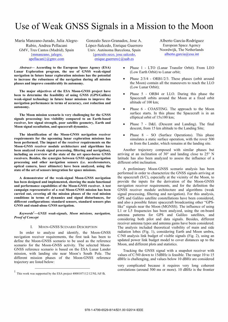
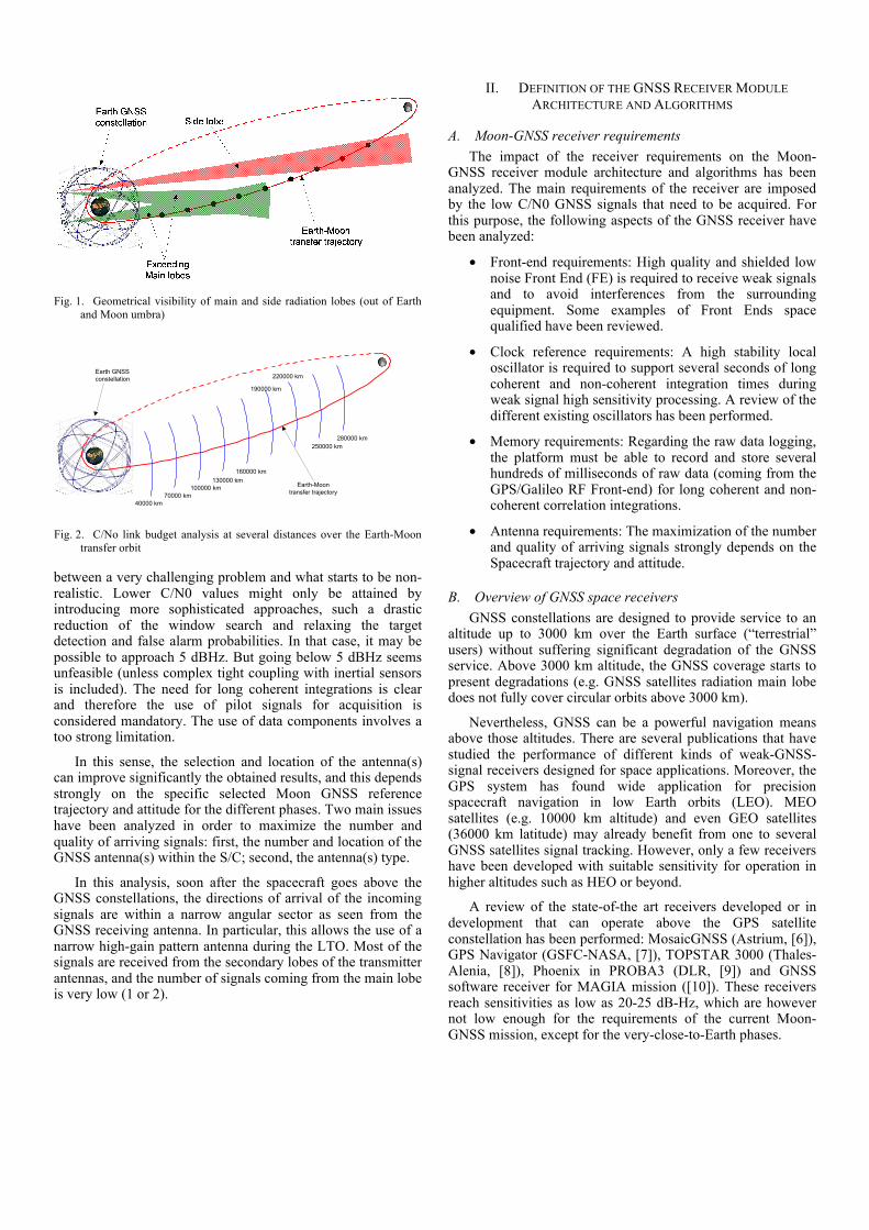
A preliminary Moon-GNSS scenario analysis has been performed in order to characterize the GNSS signals arriving at the spacecraft (S/C), especially at the vicinity of the Moon, to provide the inputs for the derivation of the Moon-GNSS navigation receiver requirements, and for the definition the GNSS receiver module architecture and algorithms (weak signal processing, filtering and navigation). For this analysis, GPS and Galileo satellite constellations have been considered, and also a possible future spacecraft broadcasting other “GPS-like” signals near the Moon (MGNSS). The influence of using L1 or L5 frequencies has been analyzed, using the on-board antenna patterns for GPS and Galileo satellites, and considering both pilot and data signals. Besides, different receiver antenna types and antenna gains have been considered. The analysis included theoretical visibility of main and side radiation lobes (Fig. 1), considering Earth and Moon umbra, C/N0 analysis link budget of visible signals (Fig. 2), using an updated power link budget model to cover distances up to the Moon, and different plots and statistics.

Tracking the GNSS signal with a snapshot receiver with values of C/N0 down to 15dBHz is feasible. The range 10 to 15 dBHz is challenging, and values below 10 dBHz are considered

very complicated because it requires very long coherent correlations (around 500 ms or more). 10 dBHz is the frontier

978-1-4799-6529-8/14/$31.00 ©2014 IEEE

between a very challenging problem and what starts to be non-realistic. Lower C/N0 values might only be attained by introducing more sophisticated approaches, such a drastic reduction of the window search and relaxing the target detection and false alarm probabilities. In that case, it may be possible to approach 5 dBHz. But going below 5 dBHz seems unfeasible (unless complex tight coupling with inertial sensors is included). The need for long coherent integrations is clear and therefore the use of pilot signals for acquisition is considered mandatory. The use of data components involves a too strong limitation.

In this sense, the selection and location of the antenna(s) can improve significantly the obtained results, and this depends strongly on the specific selected Moon GNSS reference trajectory and attitude for the different phases. Two main issues have been analyzed in order to maximize the number and quality of arriving signals: first, the number and location of the GNSS antenna(s) within the S/C; second, the antenna(s) type.

In this analysis, soon after the spacecraft goes above the GNSS constellations, the directions of arrival of the incoming signals are within a narrow angular sector as seen from the GNSS receiving antenna. In particular, this allows the use of a narrow high-gain pattern antenna during the LTO. Most of the signals are received from the secondary lobes of the transmitter antennas, and the number of signals coming from the main lobe is very low (1 or 2).

II. DEFINITION OF THE GNSS RECEIVER MODULE ARCHITECTURE AND ALGORITHMS

A. Moon-GNSS receiver requirements The impact of the receiver requirements on the Moon-

GNSS receiver module architecture and algorithms has been analyzed. The main requirements of the receiver are imposed by the low C/N0 GNSS signals that need to be acquired. For this purpose, the following aspects of the GNSS receiver have been analyzed:

• Front-end requirements: High quality and shielded low noise Front End (FE) is required to receive weak signals and to avoid interferences from the surrounding equipment. Some examples of Front Ends space qualified have been reviewed.

• Clock reference requirements: A high stability local oscillator is required to support several seconds of long coherent and non-coherent integration times during weak signal high sensitivity processing. A review of the different existing oscillators has been performed.

• Memory requirements: Regarding the raw data logging, the platform must be able to record and store several hundreds of milliseconds of raw data (coming from the GPS/Galileo RF Front-end) for long coherent and non-coherent correlation integrations.

• Antenna requirements: The maximization of the number and quality of arriving signals strongly depends on the Spacecraft trajectory and attitude.

B. Overview of GNSS space receivers GNSS constellations are designed to provide service to an

altitude up to 3000 km over the Earth surface (“terrestrial” users) without suffering significant degradation of the GNSS service. Above 3000 km altitude, the GNSS coverage starts to present degradations (e.g. GNSS satellites radiation main lobe does not fully cover circular orbits above 3000 km).

Nevertheless, GNSS can be a powerful navigation means above those altitudes. There are several publications that have studied the performance of different kinds of weak-GNSS-signal receivers designed for space applications. Moreover, the GPS system has found wide application for precision spacecraft navigation in low Earth orbits (LEO). MEO satellites (e.g. 10000 km altitude) and even GEO satellites (36000 km latitude) may already benefit from one to several GNSS satellites signal tracking. However, only a few receivers have been developed with suitable sensitivity for operation in higher altitudes such as HEO or beyond.

A review of the state-of-the art receivers developed or in development that can operate above the GPS satellite constellation has been performed: MosaicGNSS (Astrium, [6]), GPS Navigator (GSFC-NASA, [7]), TOPSTAR 3000 (Thales-Alenia, [8]), Phoenix in PROBA3 (DLR, [9]) and GNSS software receiver for MAGIA mission ([10]). These receivers reach sensitivities as low as 20-25 dB-Hz, which are however not low enough for the requirements of the current Moon-GNSS mission, except for the very-close-to-Earth phases.

Fig. 1. Geometrical visibility of main and side radiation lobes (out of Earth and Moon umbra)

40000 km

Earth GNSSconstellation

Earth-Moontransfer trajectory70000 km

100000 km130000 km

160000 km

250000 km280000 km

190000 km

220000 km

Fig. 2. C/No link budget analysis at several distances over the Earth-Moon transfer orbit

C. Architecture of GNSS receiver module An alternative way to acquire these weak signals is to use more sophisticated, higher sensitivity receivers, following the same path that led to terrestrial receivers for indoor and urban positioning. As a consequence, a snapshot architecture is selected for the receiver because it provides advantages in terms of robustness against severe signal attenuation and uncertain dynamics, and because it easily allows for long coherent and non-coherent integration intervals. Snapshot schemes are also better suited to software-defined implementations and hardware components for parallel/block processing. Moreover, it is remarkable that a snapshot / quasi open-loop architecture goes also in the direction of the Navigator development done at NASA, which hints that the use of standard closed-loop solution is not necessarily the best option [2]. The pilot components of GPS and Galileo are processed. Assistance information and INS are used to reduce the time-frequency search range. Assistance information includes also an estimation of the power of near-far interference affecting each signal.

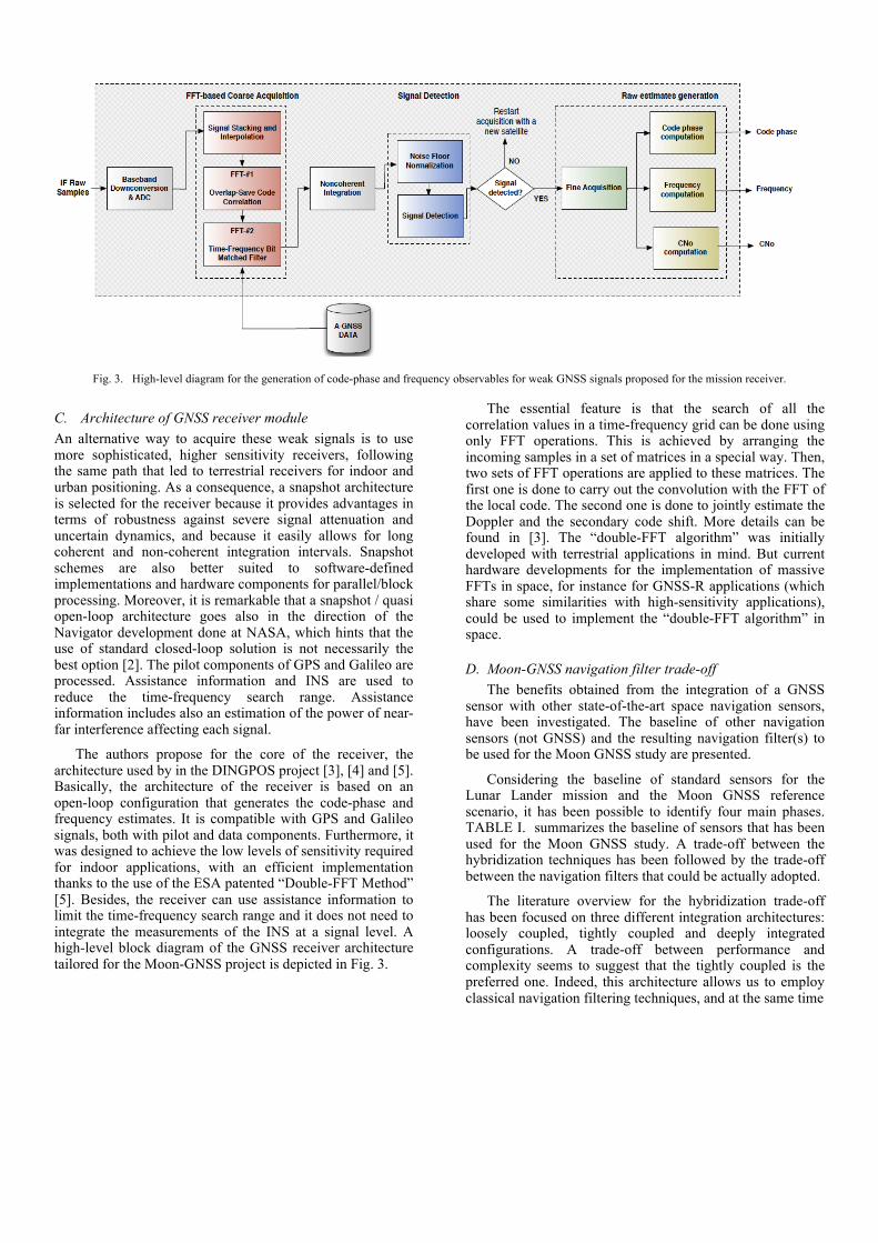
The authors propose for the core of the receiver, the architecture used by in the DINGPOS project [3], [4] and [5]. Basically, the architecture of the receiver is based on an open-loop configuration that generates the code-phase and frequency estimates. It is compatible with GPS and Galileo signals, both with pilot and data components. Furthermore, it was designed to achieve the low levels of sensitivity required for indoor applications, with an efficient implementation thanks to the use of the ESA patented “Double-FFT Method” [5]. Besides, the receiver can use assistance information to limit the time-frequency search range and it does not need to integrate the measurements of the INS at a signal level. A high-level block diagram of the GNSS receiver architecture tailored for the Moon-GNSS project is depicted in Fig. 3.

The essential feature is that the search of all the correlation values in a time-frequency grid can be done using only FFT operations. This is achieved by arranging the incoming samples in a set of matrices in a special way. Then, two sets of FFT operations are applied to these matrices. The first one is done to carry out the convolution with the FFT of the local code. The second one is done to jointly estimate the Doppler and the secondary code shift. More details can be found in [3]. The “double-FFT algorithm” was initially developed with terrestrial applications in mind. But current hardware developments for the implementation of massive FFTs in space, for instance for GNSS-R applications (which share some similarities with high-sensitivity applications), could be used to implement the “double-FFT algorithm” in space.

D. Moon-GNSS navigation filter trade-off The benefits obtained from the integration of a GNSS

sensor with other state-of-the-art space navigation sensors, have been investigated. The baseline of other navigation sensors (not GNSS) and the resulting navigation filter(s) to be used for the Moon GNSS study are presented.

Considering the baseline of standard sensors for the Lunar Lander mission and the Moon GNSS reference scenario, it has been possible to identify four main phases. TABLE I. summarizes the baseline of sensors that has been used for the Moon GNSS study. A trade-off between the hybridization techniques has been followed by the trade-off between the navigation filters that could be actually adopted.

The literature overview for the hybridization trade-off has been focused on three different integration architectures: loosely coupled, tightly coupled and deeply integrated configurations. A trade-off between performance and complexity seems to suggest that the tightly coupled is the preferred one. Indeed, this architecture allows us to employ classical navigation filtering techniques, and at the same time

Fig. 3. High-level diagram for the generation of code-phase and frequency observables for weak GNSS signals proposed for the mission receiver.

will use every single measurement from GNSS. This is fundamental, considering that the analysis in the visibility of GNSS satellites showed that 4 satellites are not visible for most of the time. Furthermore, using this configuration, it is possible to directly compare the results of the navigation algorithm with and without the GNSS system.

Regarding the navigation filter selection, and considering the comparison between the filters, a modified EKF (Extended Kalman Filter) filter has been selected. The modification consists in including the GNSS measurements in a dedicated second update block. The choice has been driven by the criteria of saving computational resources and of using consolidated and tested architecture for the state estimation using GNSS signals.

III. PROOF OF CONCEPT DESCRIPTION A Proof-of-Concept (PoC) demonstrator of the weak-

signal Moon-GNSS navigation has been implemented. The PoC is a simulator developed in Matlab/Simulink and composed by three different modules:

• Scenario Generator Module (SGM): This module is in charge of simulating the scenario characteristics and the received GNSS signals values (GNSS constellations, S/C dynamics for the different scenario phases, relative geometry between the GNSS constellations and S/C, Earth and Moon signal occultation, direction of the different GNSS signals arriving to the S/C, visibility and power link budget).

• GNSS Receiver Module (GRM): This block implements a Raw Observable Generator (ROG) whose main objective is to generate fractional pseudoranges and frequency observables with the same performance as a real receiver, taking as input the results from the SGM.

• Navigation Filter Module (NFM): This module is in charge of implementing a navigation filter taking as inputs the GNSS Receiver Module observables (pseudoranges and frequency observables) and the outputs from the different sensors used in every phase of the mission.

A. Scenario Generation Module (SGM) Its main output results are:

• Range distance from the spacecraft to the different navigation satellites;

• Doppler expected values in the GNSS signals in reception;

• C/N0 values of the GNSS signals reaching the spacecraft.

To obtain all these results, the simulator implements orbit propagators, attitude determination, link budget calculations, and antenna radiation diagrams. For the calculation of the power of the GNSS signals that would arrive to an on-board SC receiver, the power link budget model takes into account the following effects: the Earth and Moon blinding occultation, the transmission and receiver gains, free-space losses, atmospheric and other losses, etc., and this is done for different types of signals (GPS L5, GPS L1C, Galileo-E1 and Galileo-E5a signals). The SC antenna off-boresight angles to the NS satellites (obtained from the SC position and attitude, and the GNSS satellite positions) are used to compute the gain in reception according to the antenna radiation diagram.

B. GNSS Receiver Module (GRM) This block generates observables that incorporate the

effect of near-far interference and the noise in terms of acquisition probability and estimation accuracy. The ROG relies on a combination of analytical and numerical models that have been previously fitted to the results of sample-level simulations. But, the fact that the block avoids the generation of the observables using sample-level simulation reduces dramatically the execution time and allows for the analysis of long periods of time at a speed much faster than real-time. The high-level functionality of the GRM can be divided in two main parts:

• Data handling and configuration: This part handles the data present in the input file (from the SGM) for all time instants, satellites and antennas according to the chosen GRM configuration in order to select the signals from which the observables will be generated. The GRM can be configured to select the signal from the antenna with the highest C/N0 or from the antenna with the lowest near-far ratio (NFR). It also allows for enabling or disabling the near-far mitigation and for setting global and per-phase C/N0 thresholds. Furthermore, for each mission phase, it is possible to let the receiver select the best coherent and non-coherent correlation configuration based on the C/N0 or to force a given configuration.

TABLE I. BASELINE SENSORS (NOT GNSS) FOR THE DIFFERENT SCENARIO PHASES FOR THE MOON GNSS STUDY

Scenario phase

Sensors used in Attitude Dynamic

Sensors used in Translational Dynamic

LTO -Gyros -Star Tracker

-Accelerometers -Ground tracking (when available) -Orbital Propagator

LLO -Gyros -Star Tracker

-Accelerometers -Ground tracking (when available) -Orbital Propagator

COASTING -Gyros -Star Tracker

-Accelerometers -Ground tracking (when available) -Orbital Propagator -Optical camera

D&L -Gyros -Star Tracker (when available)

-Accelerometers -Ground tracking (when available) -Orbital Propagator -Optical camera -Laser Altimeter

8 9 10 11 12 13 14 15 16 17 18 19 20 21 22 23 24100

101

102

STD

in d

ista

nce

units

(m)

C/N0 (dBHz)

L1 band − Pseudorange estimation performance

Tcoh=1000ms, Ni=10Tcoh=500ms, Ni=10Tcoh=100ms, Ni=10σpRange@Tcoh=1000ms, Ni=10σpRange@Tcoh=500ms, Ni=10σpRange@Tcoh=100ms, Ni=10

8 9 10 11 12 13 14 15 16 17 18 19 20 21 22 23 24

10−1

100

101

STD

in d

ista

nce

units

(m)

C/N0 (dBHz)

L5 band − Pseudorange estimation performance

Tcoh=1000ms, Ni=10Tcoh=500ms, Ni=10Tcoh=100ms, Ni=10σpRange@Tcoh=1000ms, Ni=10σpRange@Tcoh=500ms, Ni=10σpRange@Tcoh=100ms, Ni=10

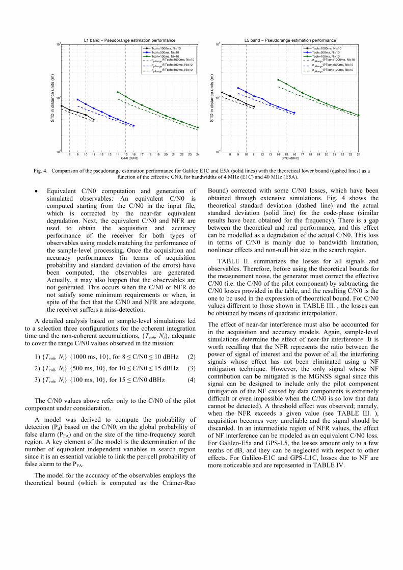
Fig. 4. Comparison of the pseudorange estimation performance for Galileo E1C and E5A (solid lines) with the theoretical lower bound (dashed lines) as a function of the effective CN0, for bandwidths of 4 MHz (E1C) and 40 MHz (E5A).

• Equivalent C/N0 computation and generation of simulated observables: An equivalent C/N0 is computed starting from the C/N0 in the input file, which is corrected by the near-far equivalent degradation. Next, the equivalent C/N0 and NFR are used to obtain the acquisition and accuracy performance of the receiver for both types of observables using models matching the performance of the sample-level processing. Once the acquisition and accuracy performances (in terms of acquisition probability and standard deviation of the errors) have been computed, the observables are generated. Actually, it may also happen that the observables are not generated. This occurs when the C/N0 or NFR do not satisfy some minimum requirements or when, in spite of the fact that the C/N0 and NFR are adequate, the receiver suffers a miss-detection.

A detailed analysis based on sample-level simulations led to a selection three configurations for the coherent integration time and the non-coherent accumulations, {Tcoh, Ni}, adequate to cover the range C/N0 values observed in the mission:

1) {Tcoh, Ni} {1000 ms, 10}, for 8 ≤ C/N0 ≤ 10 dBHz (2)

2) {Tcoh, Ni} {500 ms, 10}, for 10 ≤ C/N0 ≤ 15 dBHz (3)

3) {Tcoh, Ni} {100 ms, 10}, for 15 ≤ C/N0 dBHz (4)

The C/N0 values above refer only to the C/N0 of the pilot component under consideration.

A model was derived to compute the probability of detection (Pd) based on the C/N0, on the global probability of false alarm (PFA) and on the size of the time-frequency search region. A key element of the model is the determination of the number of equivalent independent variables in search region since it is an essential variable to link the per-cell probability of false alarm to the PFA.

The model for the accuracy of the observables employs the theoretical bound (which is computed as the Crámer-Rao

Bound) corrected with some C/N0 losses, which have been obtained through extensive simulations. Fig. 4 shows the theoretical standard deviation (dashed line) and the actual standard deviation (solid line) for the code-phase (similar results have been obtained for the frequency). There is a gap between the theoretical and real performance, and this effect can be modelled as a degradation of the actual C/N0. This loss in terms of C/N0 is mainly due to bandwidth limitation, nonlinear effects and non-null bin size in the search region.

TABLE II. summarizes the losses for all signals and observables. Therefore, before using the theoretical bounds for the measurement noise, the generator must correct the effective C/N0 (i.e. the C/N0 of the pilot component) by subtracting the C/N0 losses provided in the table, and the resulting C/N0 is the one to be used in the expression of theoretical bound. For C/N0 values different to those shown in TABLE III. , the losses can be obtained by means of quadratic interpolation.

The effect of near-far interference must also be accounted for in the acquisition and accuracy models. Again, sample-level simulations determine the effect of near-far interference. It is worth recalling that the NFR represents the ratio between the power of signal of interest and the power of all the interfering signals whose effect has not been eliminated using a NF mitigation technique. However, the only signal whose NF contribution can be mitigated is the MGNSS signal since this signal can be designed to include only the pilot component (mitigation of the NF caused by data components is extremely difficult or even impossible when the C/N0 is so low that data cannot be detected). A threshold effect was observed; namely, when the NFR exceeds a given value (see TABLE III. ), acquisition becomes very unreliable and the signal should be discarded. In an intermediate region of NFR values, the effect of NF interference can be modeled as an equivalent C/N0 loss. For Galileo-E5a and GPS-L5, the losses amount only to a few tenths of dB, and they can be neglected with respect to other effects. For Galileo-E1C and GPS-L1C, losses due to NF are more noticeable and are represented in TABLE IV.

TABLE III. SUMMARY OF NEAR-FAR EFFECT ON THE DIFFERENT SIGNALS

No

significant losses

Transition region. NF mitigation is not

necessary

Signal is recommended to be discarded unless NF can be mitigated

Galileo-E1C, GPS L1C NFR<12 dB

12 dB<NFR<27 dB (CN0 losses given by the

next table) NFR>27 dB

Galileo-E5a NFR<16 dB 16 dB<NFR<31 dB (insignificant losses) NFR>31 dB

GPS-L5 NFR<17 dB 17 dB<NFR<32 dB (insignificant losses) NFR>32 dB

TABLE IV. SUMMARY OF NEAR-FAR EFFECT ON THE DIFFERENT SIGNALS

NFR (dB) NFR < 12 12 <= NFR < 15

15 <= NFR < 20

20 <= NFR < 25

25 <= NFR <= 27

Equivalent C/N0 loss (dB) 0 0.5 1.2 1.4 1.8

C. Navigation Filter Module (NFM) The Navigation Filter Module includes two main blocks:

• Sensors: This block implements the standard set of navigation sensors according to the specifications and expected performances extracted from the Lunar Lander activity assumptions (TABLE I. ).

• Navigation: Its outputs are the S/C estimated position and velocity.

If more than 5 satellites are available, a stand-alone navigation with the GNSS signal is possible: both RLS method (Recursive Least Squares) and Peterson algorithm are implemented.

Special attention has been paid to the Surface Operations and LTO phases. The Surface operation phase starts once the S/C has landed on the Moon surface and the on-board rover begins the planetary exploration. The scope of the analysis for this phase has been to evaluate the navigation performance that could be obtained using only the GNSS signals, and then to compare the navigation accuracy to the standard requirements for rover navigation. During this phase, a Moon Surface Beacon (MSB) has been considered as another signal of the GNSS constellation, which has been fixed to the landed S/C. It has been assumed that both the S/C and rover have antenna pointing mechanisms allowing the use of high gain antennas for the GNSS signals (based on assumptions from the Lunar Lander mission), while the MGNSS and the MSB signals are received by low gain antennas. It is important to remark that the analysis with this configuration showed that more than 5 satellites are always visible, so that a stand-alone navigation with the GNSS signal is possible.

IV. TEST CAMPAIGN. FUNCTIONAL AND PERFORMANCE RESULTS

A test plan representative of a real Moon-GNSS mission covering all the mission phases representative of the real mission conditions in terms of dynamics and signal disturbances has been proposed. For this purpose, the following parameters have been identified:

• 8 mission phases.

• Signals at two different frequency bands (L1, L5).

• Presence of GNSS signals: the analysis includes navigation with and without GNSS signals. If the GNSS signals are not present the navigation considers only the standard sensors for the Lunar Lander mission (TABLE I. ).

• Possible use of MGNSS: During the test campaign the optimum MGNSS constellation has been analyzed, to improve the geometric conditions of the arriving signals and to minimize the near-far effect.

• Ground tracking measurements update period: thanks to the GNSS measurements it should be possible to reduce the Ground Tracking update.

• GNSS receiver module parameters: the correlation duration; a sensibility analysis of the assistance information uncertainty for the signal acquisition is performed; the best strategy to choose the receiving antenna for each signal is evaluated.

The test cases are structured as follows:

• The first case aims at selecting the frequency band for the GNSS signals (L1 or L5).

• The second case objective is to select the optimum MGNSS transmission power (near-far effect).

• The third case aims at evaluating the performances with infrequent ground tracking measurements.

• The fourth case aims at evaluating what is the best strategy for the selection of the receiving antenna.

• The fifth case aims at performing the sensibility analysis of the GNSS receiver to the given uncertainty window in position and velocity.

• The rest of the cases evaluate the performances of the Moon-GNSS receiver covering all the mission phases and under different conditions.

TABLE II. C/N0 LOSSES EXPERIENCED BY THE CODE-PHASE AND FREQUENCY ESTIMATION ALGORITHMS FOR THE DIFFERENT RECEIVER CONFIGURATIONS

{Tcoh, Ni} {1000 ms, 10} {500 ms, 10} {100 ms, 10} C/N0 (dBHz) 8 9 10 10 11 12 13 14 15 15 16 17 18 19 20 21 22 23 ≥24

C/N0 loss (dB) pRange@E1C, L1C 1.3 1.1 1.0 1.5 1.3 1.0 1.0 1.0 1.0 2.3 1.8 1.6 1.4 1.2 1.1 1.05 1.0 1.0 1.0

C/N0 loss (dB) pRange@ E5a,L5 1.4 1.2 0.8 1.6 1.5 1.4 0.8 0.75 0.75 2.4 2.0 1.5 1.2 1.0 0.9 0.8 0.75 0.75 0.75

C/N0 loss (dB) vel@{E1C, L1, E5a. L5} 2.3 2.1 1.8 2.8 2.5 2.0 2.0 2.0 2.0 4.5 3.5 3.0 2.5 2.2 2.0 1.7 1.4 1.25 1.0

The receiver can employ two operating modes:

• Fixing the integration time to a value for all the signals received during a mission phase.

• Selecting the integration time as a function of the expected C/N0.

Fixing the receiver integration time simplifies considerably its management. The configurations that integrate 1 second (10 non-coherent integrations of 100 ms) and 5 seconds (10 non-coherent integrations of 500 ms) facilitate implementation. Moreover, it has been corroborated that with only these two configurations it is possible to satisfy the overall mission requirements, avoiding the configuration of 10 seconds (10 non-coherent integrations of 1000 ms), which is very challenging from an implementation point of view.

This study has carefully evaluated the hybrid, standard and stand-alone GNSS navigation performances. The “standard” navigation algorithm is an EKF that considers the nominal sensors for the Lunar Lander mission, while the hybridization filter consists in an EKF with a second update (LS) that takes into account the GNSS measurements. Also a stand-alone GNSS navigation has been considered, in order to evaluate the possibility to avoid/limit the adoption of standard sensors.

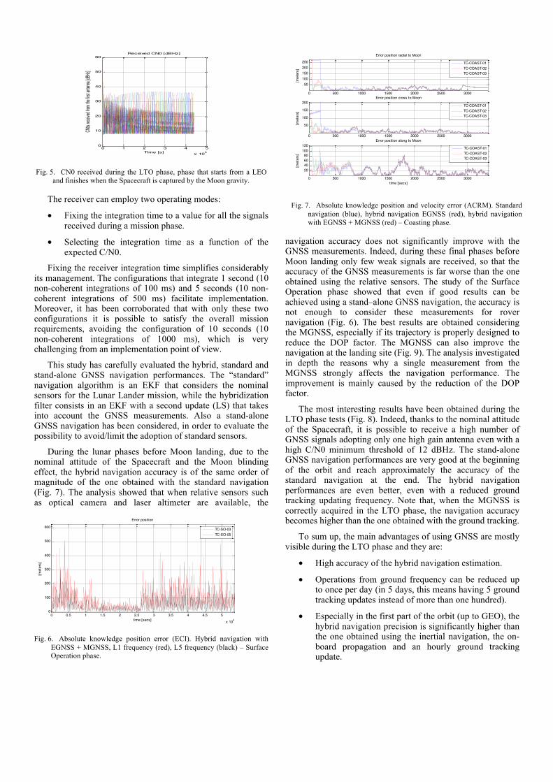
During the lunar phases before Moon landing, due to the nominal attitude of the Spacecraft and the Moon blinding effect, the hybrid navigation accuracy is of the same order of magnitude of the one obtained with the standard navigation (Fig. 7). The analysis showed that when relative sensors such as optical camera and laser altimeter are available, the

navigation accuracy does not significantly improve with the GNSS measurements. Indeed, during these final phases before Moon landing only few weak signals are received, so that the accuracy of the GNSS measurements is far worse than the one obtained using the relative sensors. The study of the Surface Operation phase showed that even if good results can be achieved using a stand–alone GNSS navigation, the accuracy is not enough to consider these measurements for rover navigation (Fig. 6). The best results are obtained considering the MGNSS, especially if its trajectory is properly designed to reduce the DOP factor. The MGNSS can also improve the navigation at the landing site (Fig. 9). The analysis investigated in depth the reasons why a single measurement from the MGNSS strongly affects the navigation performance. The improvement is mainly caused by the reduction of the DOP factor.

The most interesting results have been obtained during the LTO phase tests (Fig. 8). Indeed, thanks to the nominal attitude of the Spacecraft, it is possible to receive a high number of GNSS signals adopting only one high gain antenna even with a high C/N0 minimum threshold of 12 dBHz. The stand-alone GNSS navigation performances are very good at the beginning of the orbit and reach approximately the accuracy of the standard navigation at the end. The hybrid navigation performances are even better, even with a reduced ground tracking updating frequency. Note that, when the MGNSS is correctly acquired in the LTO phase, the navigation accuracy becomes higher than the one obtained with the ground tracking.

To sum up, the main advantages of using GNSS are mostly visible during the LTO phase and they are:

• High accuracy of the hybrid navigation estimation.

• Operations from ground frequency can be reduced up to once per day (in 5 days, this means having 5 ground tracking updates instead of more than one hundred).

• Especially in the first part of the orbit (up to GEO), the hybrid navigation precision is significantly higher than the one obtained using the inertial navigation, the on-board propagation and an hourly ground tracking update.

0 1 2 3 4 5

x 105

0

10

20

30

40

50

60Received CN0 [dBHz]

CN0s

receiv

ed from

the firs

t anten

na [dB

Hz]

Time [s]0 1 2 3 4 5

x 105

5

10

15

20

25

30

35

40

45

50

55Received CN0 [dBHz]

CN0s

receiv

ed from

the se

cond a

ntenna

[dBHz]

Time [s]0 1 2 3 4 5

x 105

5

10

15

20

25

30

35

40

45

50

55Received CN0 [dBHz]

CN0s

receiv

ed from

the thi

rd ante

nna [dB

Hz]

Time [s]

Fig. 5. CN0 received during the LTO phase, phase that starts from a LEO and finishes when the Spacecraft is captured by the Moon gravity.

0 0.5 1 1.5 2 2.5 3 3.5 4 4.5 5

x 104

0

100

200

300

400

500

600

Error position

time [secs]

[met

ers]

TC-SO-03TC-SO-05

Fig. 6. Absolute knowledge position error (ECI). Hybrid navigation with EGNSS + MGNSS, L1 frequency (red), L5 frequency (black) – Surface Operation phase.

0 500 1000 1500 2000 2500 3000

50100150200250

Error position radial to Moon

[met

ers]

0 500 1000 1500 2000 2500 3000

50

100

150

200Error position cross to Moon

[met

ers]

0 500 1000 1500 2000 2500 3000

20406080

100120

Error position along to Moon

time [secs]

[met

ers]

TC-COAST-01TC-COAST-02TC-COAST-03

TC-COAST-01TC-COAST-02TC-COAST-03

TC-COAST-01TC-COAST-02TC-COAST-03

Fig. 7. Absolute knowledge position and velocity error (ACRM). Standard navigation (blue), hybrid navigation EGNSS (red), hybrid navigation with EGNSS + MGNSS (red) – Coasting phase.

It is important to highlight that the accuracy obtained using only the GPS and Galileo satellites from Earth satisfies the mission requirements during the LTO phase. This means that the conclusions above are still valid even without the MGNSS and with only one High Gain Antenna on the Spacecraft.

V. CONCLUSIONS An analysis and identification of the navigation receiver

requirements for the upcoming lunar exploration missions has been performed. The selected Moon-GNSS reference scenario is based on the ESA Lunar Lander mission. An extensive Moon-GNSS scenario analysis has been performed in order to provide with the due inputs for the derivation of the Moon-GNSS navigation receiver requirements, and for the definition the GNSS receiver module architecture and algorithms (weak signal processing, filtering and navigation). The impact of the receiver requirements on the Moon-GNSS receiver module architecture and algorithms has been analyzed.

The architecture of the proposed GNSS receiver module relied on an open-loop configuration that generates the code-phase and frequency estimates. It is based on the ESA patented “Double-FFT” method, well-suited for an efficient implementation and very low C/N0 values. The benefits of the integration of GNSS with other state-of-the-art space navigation sensors have been analyzed. Using the developed simulator, a test campaign has been carried out covering all the mission phases. Results have been presented and confirmed the great potential of GNSS in missions to the Moon.

REFERENCES [1] The European Lunar Lander Mission. Alain Pradier. ASTRA., 12th

April 2011. [2] L. Winternitz, M. Moreau, G. Boegner, S. Sirotzky, “Navigator GPS

Receiver for Fast Acquisition and Weak Space Applications”, ION GNSS 2004.

[3] D. Kubrak, G. Seco-Granados, J. A. Lopez-Salcedo, J. L. Vicario, E. Aguado, "TN2: Technological challenges and state-of-the-art indoor positioning survey document” DINGPOS project, Oct 2007.

[4] M. Monnerat, D. Kubrak, Y. Capelle, G. Seco-Granados, J. A. Lopez-Salcedo, J. L. Vicario, I. Fernández, A. Consoli, T. Ferreira, "TN3: Platform architectural design and performance justification", DINGPOS project, Nov 2007.

[5] G. Seco-Granados, J.A. Lopez-Salcedo, D. Jimenez-Banos, G. Lopez-Risueno, "Challenges in Indoor Global Navigation Satellite Systems: Unveiling its core features in signal processing," IEEE Signal Processing Magazine, vol.29, no.2, pp.108,131, March 2012.

[6] http://www.astrium.eads.net/en/equipment/mosaicgnss-receiver.html [7] http://itpo.gsfc.nasa.gov/wp-

content/uploads/gsc_14793_1_navigator.pdf [8] TOPSTAR 3000 – An Enhanced GPS Receiver for Space Applications.

http://www.esa.int/esapub/bulletin/bullet104/gerner104.pdf [9] http://www.dlr.de/rb/desktopdefault.aspx/tabid-4736/ [10] G. Pirazzi, N. De Quattro, C. Dionisio, “GNSS software receiver for the

MAGIA (Missione Altimetrica Geofisica Geochimica lunAre) mission”, Experimental Astronomy, vol. 32, November 2011

0.5 1 1.5 2 2.5 3 3.5

x 105

500

1000

1500

2000

2500

3000Error position

Distance from Earth [km]

[met

ers]

0.5 1 1.5 2 2.5 3 3.5

x 105

50

100

150

200

250

Error velocity

Distance from Earth [km]

[met

ers/

s]

0.5 1 1.5 2 2.5 3 3.5

x 105

200

400

600

800

1000Error position

Distance from Earth [km]

[met

ers]

0.5 1 1.5 2 2.5 3 3.5

x 105

0.5

1

1.5

2

Error velocity

Distance from Earth [km]

[met

ers/

s]

Fig. 8. Absolute knowledge position and velocity errors (ECI). GNSS stand-alone navigation (top), hybrid GNSS + standard sensors navigation (bottom) – LTO phase.

0 100 200 300 400 500 600 700 800

1020304050

Error position radial to Moon

[met

ers]

0 100 200 300 400 500 600 700 800

10

20

30

40Error position cross to Moon

[met

ers]

0 100 200 300 400 500 600 700 800

50

100

150

Error position along to Moon

time [secs]

[met

ers]

TC-DL-03TC-DL-05

TC-DL-03TC-DL-05

TC-DL-03TC-DL-05

0 100 200 300 400 500 600 700 800

0.2

0.4

0.6

0.8Error velocity radial to Moon

[met

ers/

s]

0 100 200 300 400 500 600 700 800

0.20.40.60.8

Error velocity cross to Moon

[met

ers/

s]

0 100 200 300 400 500 600 700 800

0.5

1

1.5

Error velocity along to Moon

time [secs]

[met

ers/

s]

TC-DL-03TC-DL-05

TC-DL-03TC-DL-05

TC-DL-03TC-DL-05

Fig. 9. Absolute knowledge position and velocity error (ACRM). Standard navigation (blue), hybrid navigation with a dedicated MGNSS orbit (red) – D&L phase