i

COVER

URBAN SPRAWL ANALYSIS AND MODELING IN ASMARA, ERITREA:

APPLICATION OF GEOSPATIAL TOOLS

Mussie Ghebretinsae Tewolde

M

ii

URBAN SPRAWL ANALYSIS AND MODELING

IN ASMARA, ERITREA: APPLICATION OF GEOSPATIAL TOOLS

TITLE PAGE

Dissertation supervised by:

Prof. Dr. Edzer Pebesma

Co-supervisors:

Prof. Dr. Pedro Cabral, Ph.D.

Prof. Dr. Filiberto Pla, Ph.D.

Dr. Thomas Kohler

February 2011

iii

ACKNOWLEDGMENTS

First and foremost, I thank God the Almighty. I am much obliged to all my supervisors Prof. Dr. Edzer Pebesma, Prof. Dr. Pedro Cabral, Prof. Dr. Filiberto Pla and Dr. Thomas Kohler for their valuable comments, discussions and guidelines provided me during the thesis work. I would like to take the opportunity to express my appreciation and gratitude to the European Union and Erasmus Mundus Consortium (Universidade Nova de Lisboa, Portugal; Westfälische Wilhelms-Universität Münster, Germany and Universitat Jaume I, Spain) for awarding me the scholarship to undertake this course. I am grateful to the following institutions: My home institute, Hamelmalo Agricultural College for the permission granted me to study abroad. The Ministry of Land, Water and Environment; Asmara Department of Infrastructure; and Center for Development and Environment (CDE), Switzerland for providing me data and satellite images for this study. Thanks also go to the following individuals who played a part in my thesis: Tecle Yemane for his helpful information during the field visit around Asmara; Medhanie Teklemariam, Head Urban Planning Division for the information he shared me; Dr. Zemenfes Tsighe and Dr. Woldeselassie Ogbazghi for their advices during proposal development of this thesis. Tecle Tesfai and Mulugeta DoL, MLWE Eritrea. Christian Hergarten and Dr.

Sandra Eckert for their feedback.

I would also like to thank my friend Yikalo Hayelom for the discussions and chatting we had during his busy schedule. I am grateful to all Erasmus Mundus 2009 intake classmates and, to all the friends in Alfredo Sausa, Lisbon, Portugal for all the social gatherings and cheerful events. Finally, deepest gratitude goes to my beloved parents and brothers for their continuous moral support, encouragements and care.

iv

Urban Sprawl Analysis and Modeling in Asmara, Eritrea: Application of Geospatial Tools

ABSTRACT

Urbanization pattern of Greater Asmara Area for the last two decades (1989 to

2009) and a prediction for the coming ten years was studied. Satellite images and

geospatial tools were employed to quantify and analyze the spatiotemporal urban

land use changes during the study periods. The principal objective of this thesis was

to utilize satellite data, with the application of geospatial and modeling tools for

studying urban land use change. In order to achieve this, satellite data for three

study periods (1989, 2000 and 2009) have been obtained from USGS. Object-Based

Image Analysis (OBIA); and image classification with Nearest Neighbor algorithm in

eCognition Developer 8 have been accomplished. In order to assess the validation

of the classified LULC maps, Kappa measure of agreement has been used; results

were above minimum and acceptable level. ArcGIS and IDRISI Andes have been

employed for LUCC quantification; spatiotemporal analysis of the urban land use

classes; to examine the land use transitions of the land classes and identify the

gains and losses in relation to built up area; and

to characterize impacts of the

changes. Since, the major concern of the study was urban expansion, the LULC

classes were reclassified in to built up and non-built up for further analysis. Urban

sprawl has been measured using Shannon Entropy approach; results indicated the

urban area has undergone a considerable sprawl. Finally, LCM has been used to

develop a model, asses the prediction capacity of the developed model and predict

future urban land use change of the GAA. Multi-layer perceptron Neural Network

has been used to model the transition potential maps, results were successful to

make ‘actual’ prediction with Markov Chain Analyst. Despite the GAA is center of

development and its regional economic and social importance, its trend of growth

remains the major factor for diminishing productive land and other valuable natural

resources. The findings of the study indicated that, in the last twenty years the built

up area has tripled in size and impacted the surrounding natural environment. Thus,

the findings of this study might support decision making for sustainable urban

development of GAA.

v

KEYWORDS

Asmara

Change Detection

eCognition Definiens

Geospatial tools

Image Classification

LCM

LUCC

Modeling

Remote Sensing

Urban Sprawl

vi

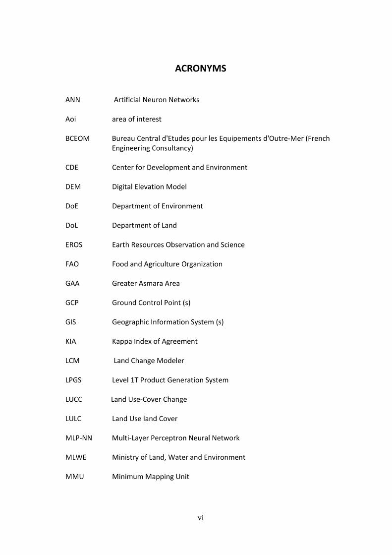
ACRONYMS ANN Artificial Neuron Networks Aoi area of interest BCEOM Bureau Central d'Etudes pour les Equipements d'Outre-Mer (French

Engineering Consultancy) CDE Center for Development and Environment DEM Digital Elevation Model DoE Department of Environment DoL Department of Land EROS Earth Resources Observation and Science FAO Food and Agriculture Organization GAA Greater Asmara Area GCP Ground Control Point (s) GIS Geographic Information System (s) KIA Kappa Index of Agreement LCM Land Change Modeler LPGS Level 1T Product Generation System LUCC Land Use-Cover Change LULC Land Use land Cover MLP-NN Multi-Layer Perceptron Neural Network MLWE Ministry of Land, Water and Environment MMU Minimum Mapping Unit

vii

MOA Ministry of Agriculture NAP National Action programme NDVI Normalized Difference Vegetation Index NN Nearest Neighbor OBIA Object-Based Image Analysis RGB Red Green Blue RMS Root Mean Square RS Remote Sensing TM Thematic Mapper UN United Nations UNFPA United Nations Population Fund USGS United States Geological Survey WRD Water Resource Department

viii

INDEX OF THE TEXT

Contents

COVER ............................................................................................................................ iTITLE PAGE .................................................................................................................... iiACKNOWLEDGMENTS .................................................................................................. iiiABSTRACT ..................................................................................................................... ivKEYWORDS .................................................................................................................... vACRONYMS .................................................................................................................. viINDEX OF THE TEXT .................................................................................................... viiiINDEX OF TABLES ......................................................................................................... xiINDEX OF FIGURES ...................................................................................................... xii

CHAPTER ONE

Introduction

1.1: Study background .......................................................................................... 11.2: Statement of the problem ............................................................................. 21.3: Study area ...................................................................................................... 41.4: Aims and objective ......................................................................................... 51.5: Research question .......................................................................................... 51.6: Significance of the study ................................................................................ 61.7: Structure of the thesis .................................................................................... 7

CHAPTER TWO

Remote Sensing: Image Classification and Analysis

2.1: Introduction .................................................................................. 82.2: Data and pre-processing ............................................................... 9

2.2.1 Data ............................................................................................................ 102.2.2 Image pre-processing ................................................................................. 11

2.3: Object Based Image classification with eCognition Developer….. 132.3.1 Classification scheme ................................................................................. 142.3.2 Image segmentation .................................................................................. 152.3.3 Training sites .............................................................................................. 172.3.4 Classification algorithm .............................................................................. 17

2.4: Classification results and validation ............................................ 192.4.1 Landuse maps ............................................................................................. 192.4.2 Classification validation .............................................................................. 19

2.5: Results and discussion ................................................................ 23

ix

CHAPTER THREE

Urban Landuse Change Detection and Urban Sprawl Analysis

3.1: Introduction ................................................................................ 243.2: Urban land use land cover change (LUCC) detection .................. 24

3.2.1 Pre-classification change detection with image difference ....................... 253.2.2. Post-classification change detection ......................................................... 26

3.3: Landuse Landcover Change Quantification and analysis ............. 273.4: LUCC in GAA and its descriptive statistical analysis ..................... 273.5: LUCC results of the GAA, analysis with Land Change Modeler .... 31

3.5.1 Greater Asmara Area (GAA) LUCC from 1989 to 2000 .............................. 323.5.2 Greater Asmara Area (GAA) LUCC from 2000 to 2009 .............................. 323.5.3 Greater Asmara Area (GAA) LUCC from 1989 to 2009 .............................. 33

3.6: Map Transition Option and Spatial Trend of Change of GAA in LCM ... 343.6.1 Map Transition Option: .............................................................................. 343.6.2 Spatial Trend of Change ............................................................................. 35

3.7: Urban sprawl measurement in G.A.A. ......................................... 363.7.1 Built up proportion in the reclassified image of the GAA .......................... 373.7.2 Shannon Entropy for sprawling measurement .......................................... 383.7.3 Urban sprawl in the GAA ............................................................................ 40

3.8: Discussion ................................................................................... 41 CHAPTER FOUR

Modeling Urban Growth Patterns

4.1: Introduction ................................................................................ 454.2: Urban land use modeling ............................................................ 464.3: Land Change Modeler (LCM) in IDRISI Andes for urban modeling ........ 474.4: Change analysis with LCM ........................................................... 474.5: Transition Potentials Modeling with LCM ................................... 48

4.5.1 Transition Sub-Model Status ...................................................................... 494.5.2 Model assumptions ..................................................................................... 494.5.3 Model variables development for GAA ..................................................... 50

4.6: Test, selection and transition of Model variables ....................... 544.7: Transition Sub-Model structure and running the model ............. 54

4.7.1 Multi-layer perceptron (MLP) neural network .......................................... 544.7.2 Running the model ..................................................................................... 55

4.8: Change prediction and validation ............................................... 574.8.1 Change prediction ...................................................................................... 574.8.2 Validation ................................................................................................... 57

x

4.9: GAA Land cover change prediction ............................................. 594.10: Results and Discussion .............................................................. 60

4.10.1 Results ...................................................................................................... 604.10.2 Discussion ................................................................................................ 62

CHAPTER FIVE

Conclusions and recommendations

5.1: Conclusions ................................................................................. 645.2: Recommendations ...................................................................... 665.3: Limitations .................................................................................. 675.4: Future Work ............................................................................... 67

Bibliography ...................................................................................... 68

Appendices ........................................................................................ 75

xi

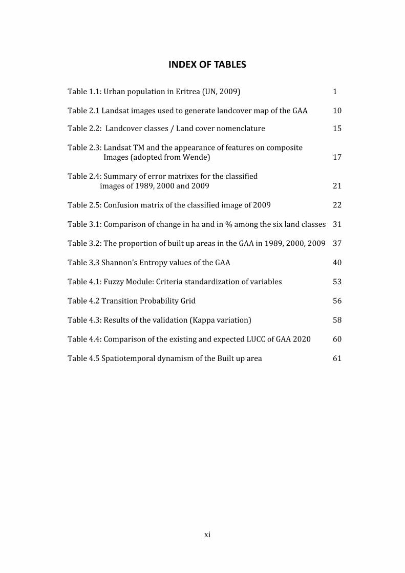
INDEX OF TABLES

Table 1.1: Urban population in Eritrea (UN, 2009) 1

Table 2.1 Landsat images used to generate landcover map of the GAA 10

Table 2.2: Landcover classes / Land cover nomenclature 15 Table 2.3: Landsat TM and the appearance of features on composite Images (adopted from Wende) 17 Table 2.4: Summary of error matrixes for the classified images of 1989, 2000 and 2009 21 Table 2.5: Confusion matrix of the classified image of 2009 22

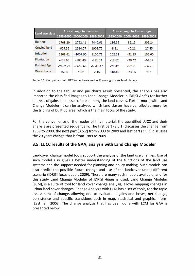
Table 3.1: Comparison of change in ha and in % among the six land classes 31

Table 3.2: The proportion of built up areas in the GAA in 1989, 2000, 2009 37 Table 3.3 Shannon’s Entropy values of the GAA 40 Table 4.1: Fuzzy Module: Criteria standardization of variables 53 Table 4.2 Transition Probability Grid 56 Table 4.3: Results of the validation (Kappa variation) 58 Table 4.4: Comparison of the existing and expected LUCC of GAA 2020 60 Table 4.5 Spatiotemporal dynamism of the Built up area 61

xii

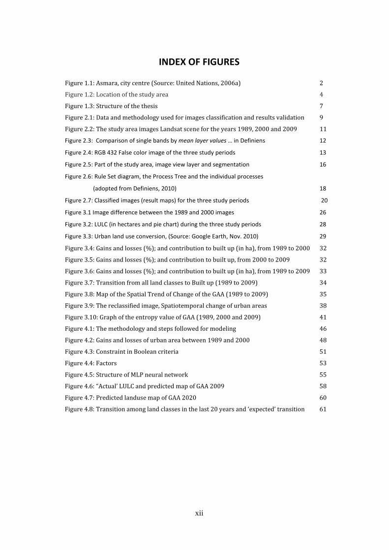
INDEX OF FIGURES Figure 1.1: Asmara, city centre (Source: United Nations, 2006a) 2

Figure 1.2: Location of the study area 4

Figure 1.3: Structure of the thesis 7

Figure 2.1: Data and methodology used for images classification and results validation 9

Figure 2.2: The study area images Landsat scene for the years 1989, 2000 and 2009 11

Figure 2.3: Comparison of single bands by mean layer values … in Definiens 12

Figure 2.4: RGB 432 False color image of the three study periods 13

Figure 2.5: Part of the study area, image view layer and segmentation 16

Figure 2.6: Rule Set diagram, the Process Tree and the individual processes

(adopted from Definiens, 2010) 18

Figure 2.7: Classified images (result maps) for the three study periods 20

Figure 3.1 Image difference between the 1989 and 2000 images 26

Figure 3.3: Urban land use conversion, (Source: Google Earth, Nov. 2010) 29

Figure 3.2: LULC (in hectares and pie chart) during the three study periods 28

Figure 3.4: Gains and losses (%); and contribution to built up (in ha), from 1989 to 2000 32

Figure 3.5: Gains and losses (%); and contribution to built up, from 2000 to 2009 32

Figure 3.6: Gains and losses (%); and contribution to built up (in ha), from 1989 to 2009 33

Figure 3.7: Transition from all land classes to Built up (1989 to 2009) 34

Figure 3.8: Map of the Spatial Trend of Change of the GAA (1989 to 2009) 35

Figure 3.9: The reclassified image, Spatiotemporal change of urban areas 38

Figure 3.10: Graph of the entropy value of GAA (1989, 2000 and 2009) 41

Figure 4.1: The methodology and steps followed for modeling 46

Figure 4.2: Gains and losses of urban area between 1989 and 2000 48

Figure 4.3: Constraint in Boolean criteria 51

Figure 4.4: Factors 53

Figure 4.5: Structure of MLP neural network 55

Figure 4.6: “Actual’ LULC and predicted map of GAA 2009 58

Figure 4.7: Predicted landuse map of GAA 2020 60

Figure 4.8: Transition among land classes in the last 20 years and ‘expected’ transition 61

1

CHAPTER ONE

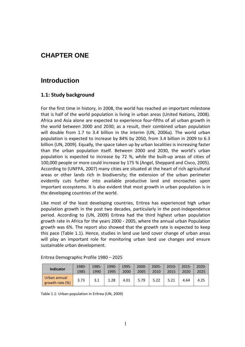
Introduction 1.1: Study background For the first time in history, in 2008, the world has reached an important milestone that is half of the world population is living in urban areas (United Nations, 2008). Africa and Asia alone are expected to experience four-fifths of all urban growth in the world between 2000 and 2030; as a result, their combined urban population will double from 1.7 to 3.4 billion in the interim (UN, 2006a). The world urban population is expected to increase by 84% by 2050, from 3.4 billion in 2009 to 6.3 billion (UN, 2009). Equally, the space taken up by urban localities is increasing faster than the urban population itself. Between 2000 and 2030, the world’s urban population is expected to increase by 72 %, while the built-up areas of cities of 100,000 people or more could increase by 175 % (Angel, Sheppard and Civco, 2005). According to (UNFPA, 2007) many cities are situated at the heart of rich agricultural areas or other lands rich in biodiversity; the extension of the urban perimeter evidently cuts further into available productive land and encroaches upon important ecosystems.

It is also evident that most growth in urban population is in the developing countries of the world.

Like most of the least developing countries, Eritrea has experienced high urban population growth in the post two decades, particularly in the post-independence period. According to (UN, 2009) Eritrea had the third highest urban population growth rate in Africa for the years 2000 - 2005, where the annual urban Population growth was 6%. The report also showed that the growth rate is expected to keep this pace (Table 1.1). Hence, studies in land use land cover change of urban areas will play an important role for monitoring urban land use changes and ensure sustainable urban development. Eritrea Demographic Profile 1980 – 2025

Table 1.1: Urban population in Eritrea (UN, 2009)

Indicator 1980-1985

1985-1990

1990-1995

1995-2000

2000-2005

2005-2010

2010-2015

2015-2020

2020-2025

Urban annual growth rate (%)

3.73 3.1 1.28 4.01 5.79 5.22 5.21 4.64 4.25

2

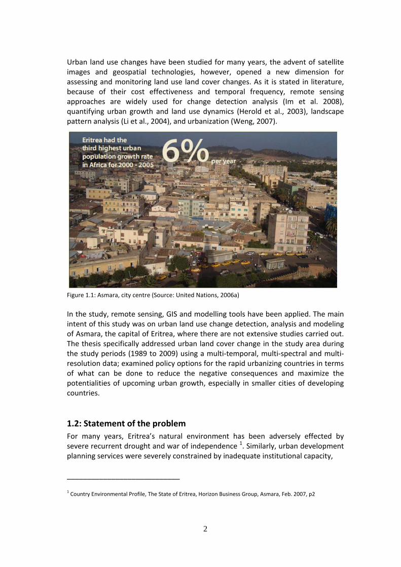
Urban land use changes have been studied for many years, the advent of satellite images and geospatial technologies, however, opened a new dimension for assessing and monitoring land use land cover changes. As it is stated in literature,

because of their cost effectiveness and temporal frequency, remote sensing approaches are widely used for change detection analysis (Im et al. 2008), quantifying urban growth and land use dynamics (Herold et al., 2003), landscape pattern analysis (Li et al., 2004), and urbanization (Weng, 2007).

Figure 1.1: Asmara, city centre (Source: United Nations, 2006a) In the study, remote sensing, GIS and modelling tools have been applied. The main intent of this study was on urban land use change detection, analysis and modeling of Asmara, the capital of Eritrea, where there are not extensive studies carried out. The thesis specifically addressed urban land cover change in the study area during the study periods (1989 to 2009) using a multi-temporal, multi-spectral and multi-resolution data; examined policy options for the rapid urbanizing countries in terms of what can be done to reduce the negative consequences and maximize the potentialities of upcoming urban growth, especially in smaller cities of developing countries. 1.2: Statement of the problem For many years, Eritrea’s natural environment has been adversely effected by severe recurrent drought and war of independence 1

. Similarly, urban development planning services were severely constrained by inadequate institutional capacity,

____________________________ 1

Country Environmental Profile, The State of Eritrea, Horizon Business Group, Asmara, Feb. 2007, p2

3

inadequate budget, human expertise and technologies. Furthermore, population growth in rural areas and related migration towards urban areas especially to the capital city Asmara is continuous as occurs elsewhere on the continent. Consequently within the study area urban sprawl took place adversely, and the city faced a number of environmental concerns including unacceptable condition of the urban environment in the unplanned settlements. These are: lack of basic infrastructure and amenities, lack of safe drinking water, inadequate sanitation facilities and inadequate management of solid waste disposals. These environmental pollutions directly impact the water sources of the city. The city is entirely dependent on surface water resources from the existing dam reservoirs (BCEOM/Groupe Huit-Optima, 2006). Recently, due to high demand of land for residential and other development activities the Central zone administration annexed thirteen satellite villages to the earlier environ of Asmara. The communities of these villages are dominantly depending on agriculture. These created land use conflict in the fringe of the urban area where there are competing demands on land for food production, industrial crops, urban expansion and industrial development.

Land is limited resource, and it is under a great pressure due to the urban expansion. The Greater Asmara Area (GAA) the main focus of this study, which is Asmara and the nearby thirteen satellite villages, is scene of intense competition between housing and agricultural land uses. It is indicated in the Housing/Urban Development Policy Report (2005), the MOLWE has estimated that 1980ha of agricultural land around Asmara have been taken up by urban development in the past four decades. The rhythm has accelerated between 1997 and 2002 to around 70ha per year. In the year 2004/2005, planned land allocation for ‘Tessa’2 (land for housing) and ‘BOND’3

(special lease land) was remarkably high, which is over 2500ha for urban development.

In addition to the above mentioned environmental and urban sprawl factors in the newly expanding areas, the design density is low which leads to high infrastructure cost (BCEOM/Groupe Huit-Optima, 2006), though only fraction of population will live there. During a field visit the researcher has also observed that, the irrigation lands that provide fresh vegetables food for the market are under stress. Housing expansion areas have tended to ignore the topography, hydrograph, natural site as well as fertile land. High Agricultural areas and periodically flooded area have also been built (BCEOM/Groupe Huit-Optima, 2006).

__________________________

2 Tessa land (land for housing) refers to village land that is allotted to an Eritrean whose origin is in the village.

3

‘Bond’ land is a special form of lease land. The charges for this type of land are much higher than for ordinary lease land, and have to be paid in foreign currency. It is typically available only to Eritreans in diasporas.

4

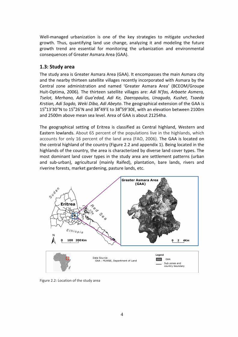
Well-managed urbanization is one of the key strategies to mitigate unchecked growth. Thus, quantifying land use change, analyzing it and modeling the future growth trend are essential for monitoring the urbanization and environmental consequences of Greater Asmara Area (GAA). 1.3: Study area The study area is Greater Asmara Area (GAA). It encompasses the main Asmara city and the nearby thirteen satellite villages recently incorporated with Asmara by the Central zone administration and named ‘Greater Asmara Area’ (BCEOM/Groupe Huit-Optima, 2006). The thirteen satellite villages are: Adi N’fas, Arbaete Asmera, Tselot, Merhano, Adi Gua’edad, Adi Ke, Daeropaulos, Unagudo, Kushet, Tsaeda Krstian, Adi Sogdo, Weki Diba, Adi Abeyto. The geographical extension of the GAA is 15o13′30′′N to 15o26’N and 38o49’E to 38o

59’30E, with an elevation between 2100m and 2500m above mean sea level. Area of GAA is about 21254ha.

The geographical setting of Eritrea is classified as Central highland, Western and Eastern lowlands. About 65 percent of the populations live in the highlands, which accounts for only 16 percent of the land area (FAO, 2006). The GAA is located on the central highland of the country (Figure 2.2 and appendix 1). Being located in the highlands of the country, the area is characterized by diverse land cover types. The most dominant land cover types in the study area are settlement patterns (urban and sub-urban), agricultural (mainly Raifed), plantation, bare lands, rivers and riverine forests, market gardening, pasture lands, etc.

Figure 2.2: Location of the study area

5

1.4: Aims and objective

The major aim of this thesis was to utilize satellite data, with the application of geospatial and modeling tools for studying urban land use-cover change.

In order to attain the major aim, the following specific objectives were also specified in sequence:

• Acquire land use maps of the urban area from satellite images classification; • Assess the accuracy of the classified images or maps using error matrix and

Kappa statistics; • Quantify the area of the defined land classes of the acquired maps • Spatial and temporal analysis among the urban land classes during the three

study time periods • Examine the land use transitions of the land classes and identify the gains

and losses of the land classes in relation to built up area. Plus characterize impacts of urban land use change on the other valuable land classes

• Examine the urban expansion with Shanonn’s entropy approach, • Develop a model, asses the prediction capacity of the model and predict

future urban land use change of the study area • Analyze the specific issues of the urban environment and put forward a

recommendations that may support decision making for a sound solution of sustainable urban growth

1.5: Research question The core question of this research was to understand how much the built up area of the GAA has grown out ward; to what extent has it impacted the productive land and the surrounding natural environment in the last two decades. What would be the impact in the coming ten years, if the situation of built up outward growth is not regulated by policy instrument? In line with the core research question, the following specific questions were set:

• How was the trend of growth of the built up areas during the three study time periods?

• How much the Built up area has grown in the last twenty tears? • How was the transition and dynamics among the defined urban land

classes? • Which land classes have expanded and at the expense of which? And how

much? • Which land uses were highly affected by urban growth? • Was the urban growth sustainable?

6

• How would be the transition of land among the urban land classes in the coming ten years?

• What were the major deriving forces for the changes? And what would be the extent of the urban land use changes in the future?

1.6: Significance of the study Although urban areas are centers of economic development, the trend of urban growth remains the major factor for diminishing valuable natural resources. Therefore, urban land use change studies are important for planning and decision making to mitigate the impacts of urban expansion and attain sustainable urban development. Thus, the findings of this study was anticipated to provide maps that show a synoptic view of the study area; that is to produce urban land use maps for the three study periods from satellite data. Thus, decision makers can easily recognize the LUCC from the results of the study presented in various maps, statistical and graphical presentations. Situation assessment of the study area with geospatial tools offers important information for land managers, urban planners, policymakers, conservation agencies and other stakeholders to play a part in policy formulation for the betterment and conservation consent urban growth. More importantly, the result of this study is significant because remote sensing has much advantage over in-situ measurement for LUCC. Landsat images used for this study area available for free; thus, make use of remote sensing saves time, energy and it is cost effective to be used by developing countries like Eritrea. Hence, the quantified and analyzed urban land use change for the last 20 years (1989 to 2009), plus the result of urban growth prediction for the coming 10 years could support in sound decision making for Sustainable development of GAA.

7

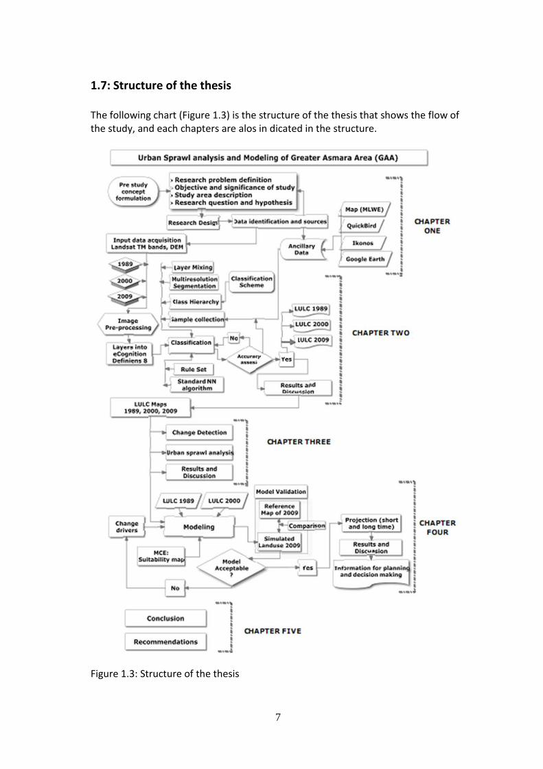
1.7: Structure of the thesis The following chart (Figure 1.3) is the structure of the thesis that shows the flow of the study, and each chapters are alos in dicated in the structure.

Figure 1.3: Structure of the thesis

8

CHAPTER TWO

Remote Sensing: Image Classification and Analysis 2.1: Introduction Remote Sensing is the non contact recording of information from the ultraviolet, visible, infrared, and microwave regions of the electromagnetic spectrum by means of instruments know as sensors Jensen (2006). Remote sensing is the science of identifying features from imagery acquired by a sensor mounted on remote platform. The digital image obtained from sensors are processed, prepared, classified and analyzed in different stages of remote sensing techniques to get information for various applications. The use of satellite imagery has made mapping of landcover more efficient and reliable. As stated by Anderson et al. (1976), one of the prime pre-requisites for better use of land is information on existing land use patterns and changes in landuse through time. Hence, in order to monitor urban growth and urban landcover dynamics, the availability of updated surface information is a pre-requisite. It provides a large variety and amount of data about the surface of the earth. Remote sensing technology has great potential for acquisition of detailed and accurate landuse information for management and planning of urban areas (Herold et al. 2002). Besides, an increasing number of remotely sensed data sources are available for detecting and characterizing urban land use change. Data can now be acquired at multiple times per day, and at spatial scales ranging from 1km to less than 1m resolution. The computational power to extract meaningful quantitative results from remotely sensed data has also improved tremendously. These developments in both data access and data processing ability present exciting and cost-effective opportunities for remote sensing approaches to be used widely in change detection analysis (Im et al. 2008). Urban LULC mapping for change detection from satellite data using various techniques has been performed by a large number of experts (Masek et al., 2000; Kaufmann, 2001; Gluch, 2002; Herold et al. 2003, Cabral, 2005; 2006). Nonetheless, it is still sometimes appeared difficult in practice to select a good change detection method (D. Lu et al. 2004). Effective image classification for urban LULC mapping and change detection depends on many factors. However, the main consideration should be given on the selection of the available multi temporal data, processing and method of image classification. In this study Object Oriented image classification approach implemented in Definiens 8 has been chosen to classify Landsat TM scenes. This chapter will be discussing about the satellite data used and their preparation and pre-processing in ERDAS Imagine 9.2; the methodology and algorithm employed for image classification in Definiens 8 and the accuracy

9

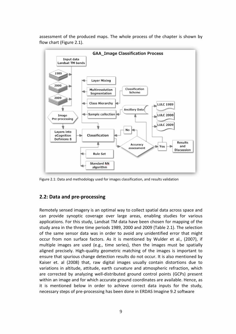
assessment of the produced maps. The whole process of the chapter is shown by flow chart (Figure 2.1).

Figure 2.1: Data and methodology used for images classification, and results validation 2.2: Data and pre-processing Remotely sensed imagery is an optimal way to collect spatial data across space and can provide synoptic coverage over large areas, enabling studies for various applications. For this study, Landsat TM data have been chosen for mapping of the study area in the three time periods 1989, 2000 and 2009 (Table 2.1). The selection of the same sensor data was in order to avoid any unidentified error that might occur from non surface factors. As it is mentioned by Wulder et al., (2007), if multiple images are used (e.g., time series), then the images must be spatially aligned precisely. High-quality geometric matching of the images is important to ensure that spurious change detection results do not occur. It is also mentioned by Kaiser et. al (2008) that, raw digital images usually contain distortions due to variations in altitude, attitude, earth curvature and atmospheric refraction, which are corrected by analyzing well-distributed ground control points (GCPs) present within an image and for which accurate ground coordinates are available. Hence, as it is mentioned below in order to achieve correct data inputs for the study, necessary steps of pre-processing has been done in ERDAS Imagine 9.2 software

10

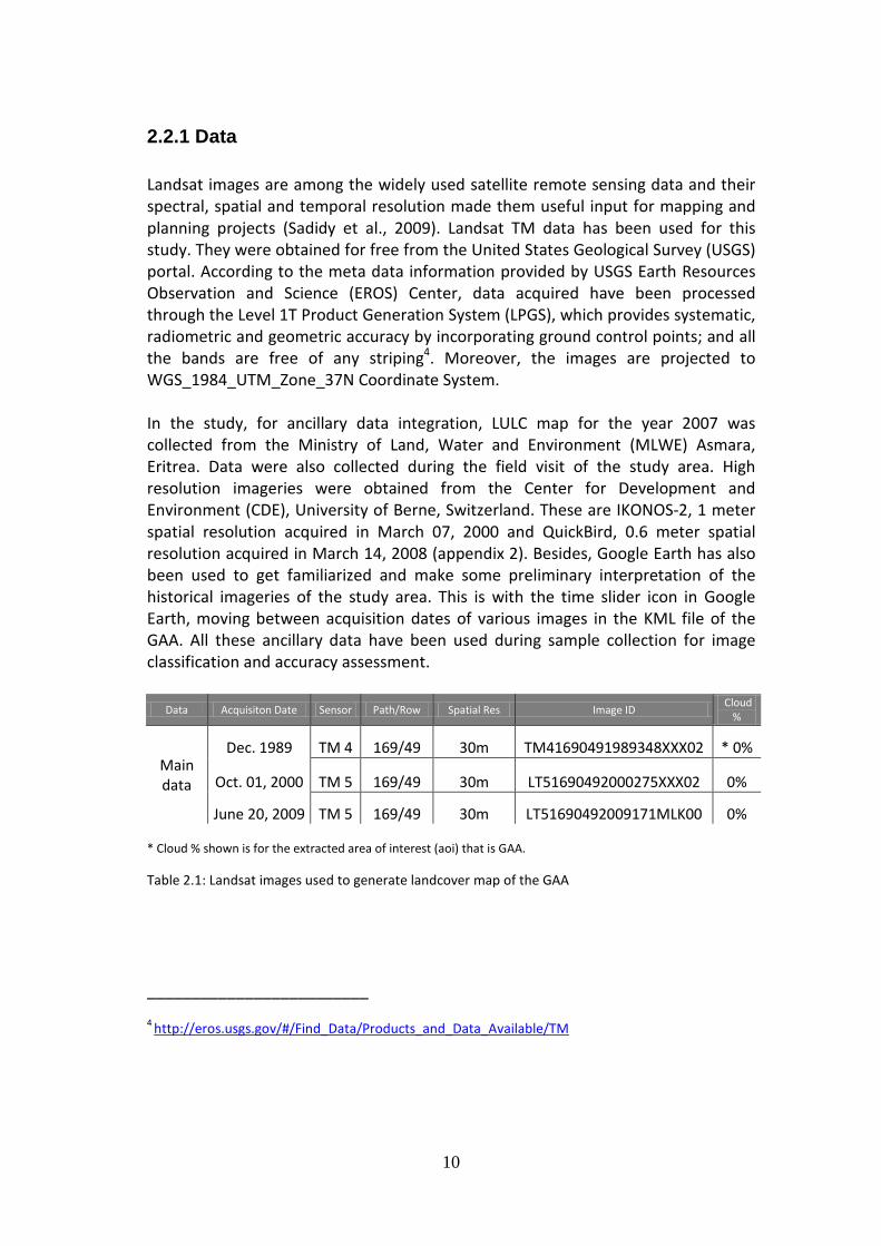
2.2.1 Data Landsat images are among the widely used satellite remote sensing data and their spectral, spatial and temporal resolution made them useful input for mapping and planning projects (Sadidy et al., 2009). Landsat TM data has been used for this study. They were obtained for free from the United States Geological Survey (USGS) portal. According to the meta data information provided by USGS Earth Resources Observation and Science (EROS) Center, data acquired have been processed through the Level 1T Product Generation System (LPGS), which provides systematic, radiometric and geometric accuracy by incorporating ground control points; and all the bands are free of any striping4

. Moreover, the images are projected to WGS_1984_UTM_Zone_37N Coordinate System.

In the study, for ancillary data integration, LULC map for the year 2007 was collected from the Ministry of Land, Water and Environment (MLWE) Asmara, Eritrea. Data were also collected during the field visit of the study area. High resolution imageries were obtained from the Center for Development and Environment (CDE), University of Berne, Switzerland. These are IKONOS-2, 1 meter spatial resolution acquired in March 07, 2000 and QuickBird, 0.6 meter spatial resolution acquired in March 14, 2008 (appendix 2). Besides, Google Earth has also been used to get familiarized and make some preliminary interpretation of the historical imageries of the study area. This is with the time slider icon in Google Earth, moving between acquisition dates of various images in the KML file of the GAA. All these ancillary data have been used during sample collection for image classification and accuracy assessment.

Data Acquisiton Date Sensor Path/Row Spatial Res Image ID Cloud

%

Main data

Dec. 1989 TM 4 169/49 30m TM41690491989348XXX02 * 0%

Oct. 01, 2000 TM 5 169/49 30m LT51690492000275XXX02 0%

June 20, 2009 TM 5 169/49 30m LT51690492009171MLK00 0% * Cloud % shown is for the extracted area of interest (aoi) that is GAA.

Table 2.1: Landsat images used to generate landcover map of the GAA _________________________

4 http://eros.usgs.gov/#/Find_Data/Products_and_Data_Available/TM

11

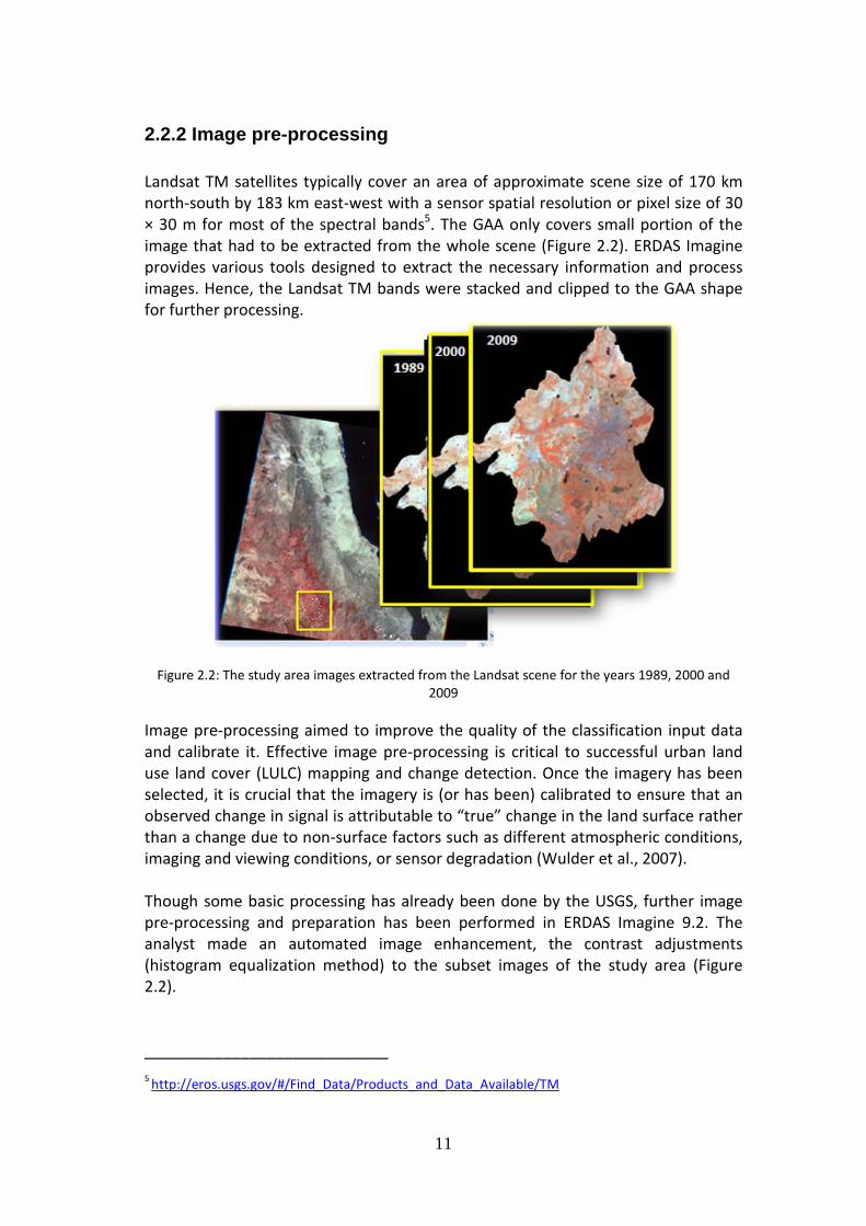
2.2.2 Image pre-processing Landsat TM satellites typically cover an area of approximate scene size of 170 km north-south by 183 km east-west with a sensor spatial resolution or pixel size of 30 × 30 m for most of the spectral bands5

. The GAA only covers small portion of the image that had to be extracted from the whole scene (Figure 2.2). ERDAS Imagine provides various tools designed to extract the necessary information and process images. Hence, the Landsat TM bands were stacked and clipped to the GAA shape for further processing.

Figure 2.2: The study area images extracted from the Landsat scene for the years 1989, 2000 and

2009

Image pre-processing aimed to improve the quality of the classification input data and calibrate it. Effective image pre-processing is critical to successful urban land use land cover (LULC) mapping and change detection. Once the imagery has been selected, it is crucial that the imagery is (or has been) calibrated to ensure that an observed change in signal is attributable to “true” change in the land surface rather than a change due to non-surface factors such as different atmospheric conditions, imaging and viewing conditions, or sensor degradation (Wulder et al., 2007). Though some basic processing has already been done by the USGS, further image pre-processing and preparation has been performed in ERDAS Imagine 9.2. The analyst made an automated image enhancement, the contrast adjustments (histogram equalization method) to the subset images of the study area (Figure 2.2).

____________________________ 5 http://eros.usgs.gov/#/Find_Data/Products_and_Data_Available/TM

12

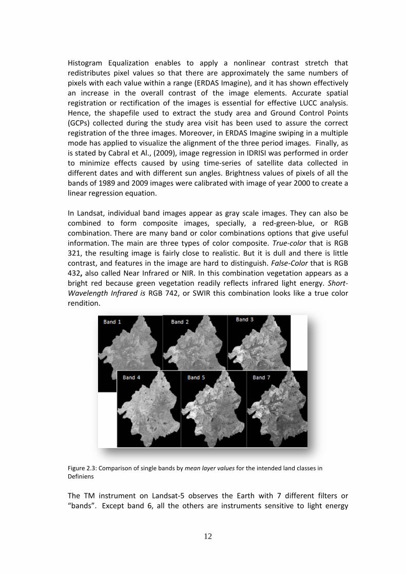
Histogram Equalization enables to apply a nonlinear contrast stretch that redistributes pixel values so that there are approximately the same numbers of pixels with each value within a range (ERDAS Imagine), and it has shown effectively an increase in the overall contrast of the image elements. Accurate spatial registration or rectification of the images is essential for effective LUCC analysis. Hence, the shapefile used to extract the study area and Ground Control Points (GCPs) collected during the study area visit has been used to assure the correct registration of the three images. Moreover, in ERDAS Imagine swiping in a multiple mode has applied to visualize the alignment of the three period images. Finally, as is stated by Cabral et Al., (2009), image regression in IDRISI was performed in order to minimize effects caused by using time-series of satellite data collected in different dates and with different sun angles. Brightness values of pixels of all the bands of 1989 and 2009 images were calibrated with image of year 2000 to create a linear regression equation. In Landsat, individual band images appear as gray scale images. They can also be combined to form composite images, specially, a red-green-blue, or RGB combination. There are many band or color combinations options that give useful information. The main are three types of color composite. True-color that is RGB 321, the resulting image is fairly close to realistic. But it is dull and there is little contrast, and features in the image are hard to distinguish. False-Color that is RGB 432, also called Near Infrared or NIR. In this combination vegetation appears as a bright red because green vegetation readily reflects infrared light energy. Short-Wavelength Infrared is RGB 742, or SWIR this combination looks like a true color rendition.

Figure 2.3: Comparison of single bands by mean layer values for the intended land classes in Definiens

The TM instrument on Landsat-5 observes the Earth with 7 different filters or “bands”. Except band 6, all the others are instruments sensitive to light energy

13

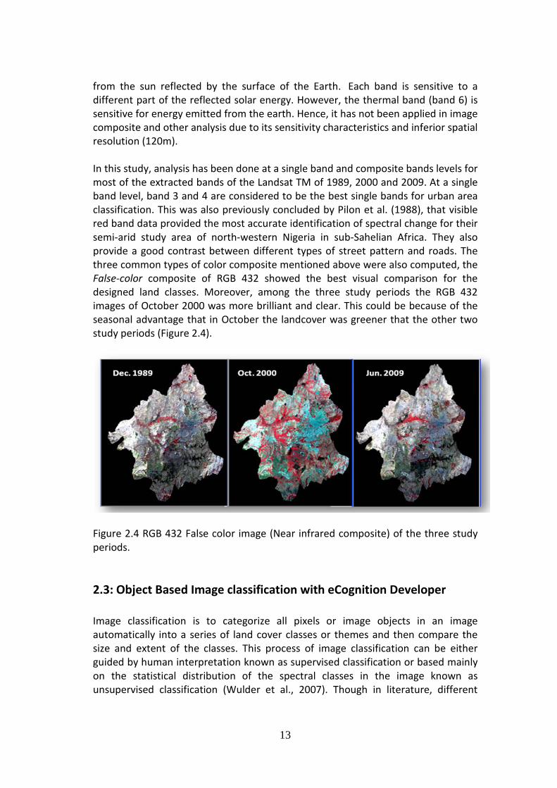
from the sun reflected by the surface of the Earth. Each band is sensitive to a different part of the reflected solar energy. However, the thermal band (band 6) is sensitive for energy emitted from the earth. Hence, it has not been applied in image composite and other analysis due to its sensitivity characteristics and inferior spatial resolution (120m). In this study, analysis has been done at a single band and composite bands levels for most of the extracted bands of the Landsat TM of 1989, 2000 and 2009. At a single band level, band 3 and 4 are considered to be the best single bands for urban area classification. This was also previously concluded by Pilon et al. (1988), that visible red band data provided the most accurate identification of spectral change for their semi-arid study area of north-western Nigeria in sub-Sahelian Africa. They also provide a good contrast between different types of street pattern and roads. The three common types of color composite mentioned above were also computed, the False-color composite of RGB 432 showed the best visual comparison for the designed land classes. Moreover, among the three study periods the RGB 432 images of October 2000 was more brilliant and clear. This could be because of the seasonal advantage that in October the landcover was greener that the other two study periods (Figure 2.4).

Figure 2.4 RGB 432 False color image (Near infrared composite) of the three study periods.

2.3: Object Based Image classification with eCognition Developer Image classification is to categorize all pixels or image objects in an image automatically into a series of land cover classes or themes and then compare the size and extent of the classes. This process of image classification can be either guided by human interpretation known as supervised classification or based mainly on the statistical distribution of the spectral classes in the image known as unsupervised classification (Wulder et al., 2007). Though in literature, different

14

classification systems are mentioned, they are generally not comparable one to another and also there is no single internationally accepted land cover classification system (Latham, 2001). The researcher in this study has choose, eCognition Definiens also known as Definiens Developer 8 for image classification due to the advantage of classifying image at image object level instead of pixel level. As it is mentioned by Araya et al., (2008) the world is not pixilated; rather it is arranged in objects. Object oriented classification avoids mixed pixel problems which usually occur in urban area studies. For example, in pixel level classification bare sand soil and the impervious parts of urban areas usual create a mixed pixel problem. eCognition Developer6

Version 8 is an image analysis software of geo-spatial information extraction from a remote sensing imagery. It is object-based image analysis (OBIA) software. It offers a range of tools to create image analysis applications that can handle all common data sources, such as medium to high resolution satellite data very high resolution aerial photography, LiDAR, radar and even hyper spectral data.

Definiens Developer is one of the three components in eCognition software product; it is the development environment for object-based image analysis. It is used to develop rule sets for the automatic analysis of remote sensing data. It incorporates a multi-resolution bottom-up region growing approach in the generation of image objects. The advantage of object-based classification is that each image object represents a definite spatially connected region of the image. The pixels of the associated region are linked to the image object. In addition to the multispectral bands, the object-based approach takes advantage of all dimensions of remote sensing including spatial (area, length, width and direction), the morphological (shape parameters, texture), contextual (relationship to neighbors, proximity analysis) and temporal (time series) (Navulur, 2007). The resulting object-based features can then be incorporated into the classification process.

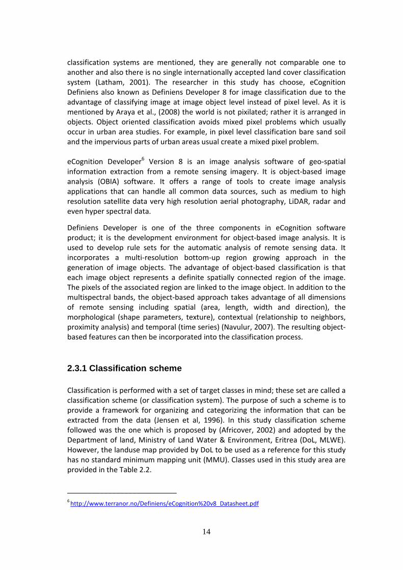
2.3.1 Classification scheme Classification is performed with a set of target classes in mind; these set are called a classification scheme (or classification system). The purpose of such a scheme is to provide a framework for organizing and categorizing the information that can be extracted from the data (Jensen et al, 1996). In this study classification scheme followed was the one which is proposed by (Africover, 2002) and adopted by the Department of land, Ministry of Land Water & Environment, Eritrea (DoL, MLWE). However, the landuse map provided by DoL to be used as a reference for this study has no standard minimum mapping unit (MMU). Classes used in this study area are provided in the Table 2.2. ___________________________ 6 http://www.terranor.no/Definiens/eCognition%20v8_Datasheet.pdf

15

The detail land classes nomenclature is simplified, as the main focus of the study is in urban areas. The first step in a supervised classification method is to identify the landcover and landuse (LULC) classes to be used. LULC terminology has an interchangeable meaning, but generally it can be said that Landcover refers to the type of material present on the site (e.g. water, crops, forest, wet land, asphalt, and concrete). Land use refers to the modifications made by people on the land cover (e.g. agriculture, commerce, settlement)11

.

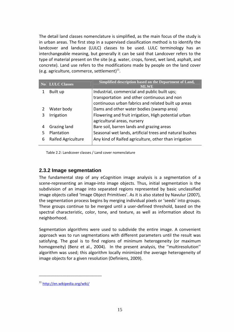
No LULC Classes Simplified description based on the Department of Land, MLWE

1 Built up Industrial, commercial and public built ups; transportation and other continuous and non continuous urban fabrics and related built up areas

2 Water body Dams and other water bodies (swamp area) 3 Irrigation Flowering and fruit irrigation, High potential urban

agricultural areas, nursery 4 Grazing land Bare soil, barren lands and grazing areas 5 Plantation Seasonal wet lands, artificial trees and natural bushes 6 Raifed Agriculture Any kind of Raifed agriculture, other than irrigation

Table 2.2: Landcover classes / Land cover nomenclature

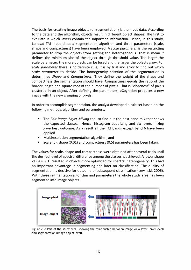
2.3.2 Image segmentation The fundamental step of any eCognition image analysis is a segmentation of a scene-representing an image-into image objects. Thus, initial segmentation is the subdivision of an image into separated regions represented by basic unclassified image objects called ‘Image Object Primitives’. As it is also stated by Navulur (2007), the segmentation process begins by merging individual pixels or ‘seeds’ into groups. These groups continue to be merged until a user-defined threshold, based on the spectral characteristic, color, tone, and texture, as well as information about its neighborhood. Segmentation algorithms were used to subdivide the entire image. A convenient approach was to run segmentations with different parameters until the result was satisfying. The goal is to find regions of minimum heterogeneity (or maximum homogeneity) (Benz et al., 2004). In the present analysis, the ‘‘multiresolution’’ algorithm was used; this algorithm locally minimized the average heterogeneity of image objects for a given resolution (Definiens, 2009).

________________________________

11 http://en.wikipedia.org/wiki/

16

The basis for creating image objects (or segmentation) is the input-data. According to the data and the algorithm, objects result in different object shapes. The first to evaluate is which layers contain the important information. Hence, in this study, Landsat TM input data; a segmentation algorithm and three parameters (scale, shape and compactness) have been employed. A scale parameter is the restricting parameter to stop the objects from getting too heterogeneous. That is mean it defines the minimum size of the object through threshold value. The larger the scale parameter, the more objects can be fused and the larger the objects grow. For scale parameter there is no definite rule, it is by trial and error to find out which scale parameter to decide. The homogeneity criterion of the segmentation is determined Shape and Compactness. They define the weight of the shape and compactness the segmentation should have. Compactness equals the ratio of the border length and square root of the number of pixels. That is "closeness" of pixels clustered in an object. After defining the parameters, eCognition produces a new image with the new grouping of pixels. In order to accomplish segmentation, the analyst developed a rule set based on the following methods, algorithm and parameters: The Edit Image Layer Mixing tool to find out the best band mix that shows

the expected classes. Hence, histogram equalizing and six layers mixing gave best outcome. As a result all the TM bands except band 6 have been applied.

Multiresolution segmentation algorithm, and Scale (5), shape (0.01) and compactness (0.5) parameters has been taken.

The values for scale, shape and compactness were obtained after several trials until the desired level of spectral difference among the classes is achieved. A lower shape value (0.01) resulted in objects more optimized for spectral heterogeneity. This had an important advantage in segmenting and later on classification. The quality of segmentation is decisive for outcome of subsequent classification (Lewinski, 2006). With these segmentation algorithm and parameters the whole study area has been segmented into image objects.

Figure 2.5: Part of the study area, showing the relationship between image view layer (pixel level) and segmentation (image object level).

17

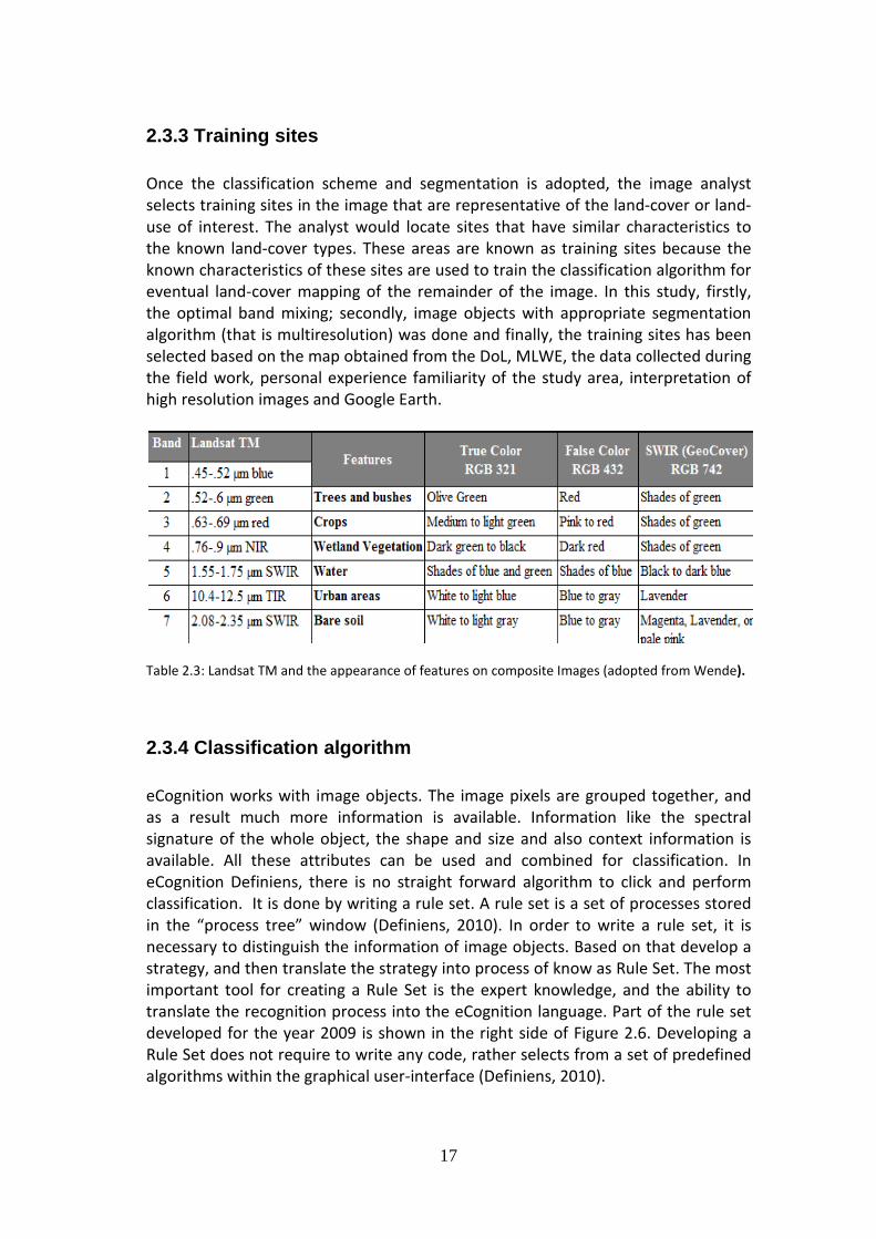
2.3.3 Training sites Once the classification scheme and segmentation is adopted, the image analyst selects training sites in the image that are representative of the land-cover or land-use of interest. The analyst would locate sites that have similar characteristics to the known land-cover types. These areas are known as training sites because the known characteristics of these sites are used to train the classification algorithm for eventual land-cover mapping of the remainder of the image. In this study, firstly, the optimal band mixing; secondly, image objects with appropriate segmentation algorithm (that is multiresolution) was done and finally, the training sites has been selected based on the map obtained from the DoL, MLWE, the data collected during the field work, personal experience familiarity of the study area, interpretation of high resolution images and Google Earth.

Table 2.3: Landsat TM and the appearance of features on composite Images (adopted from Wende).

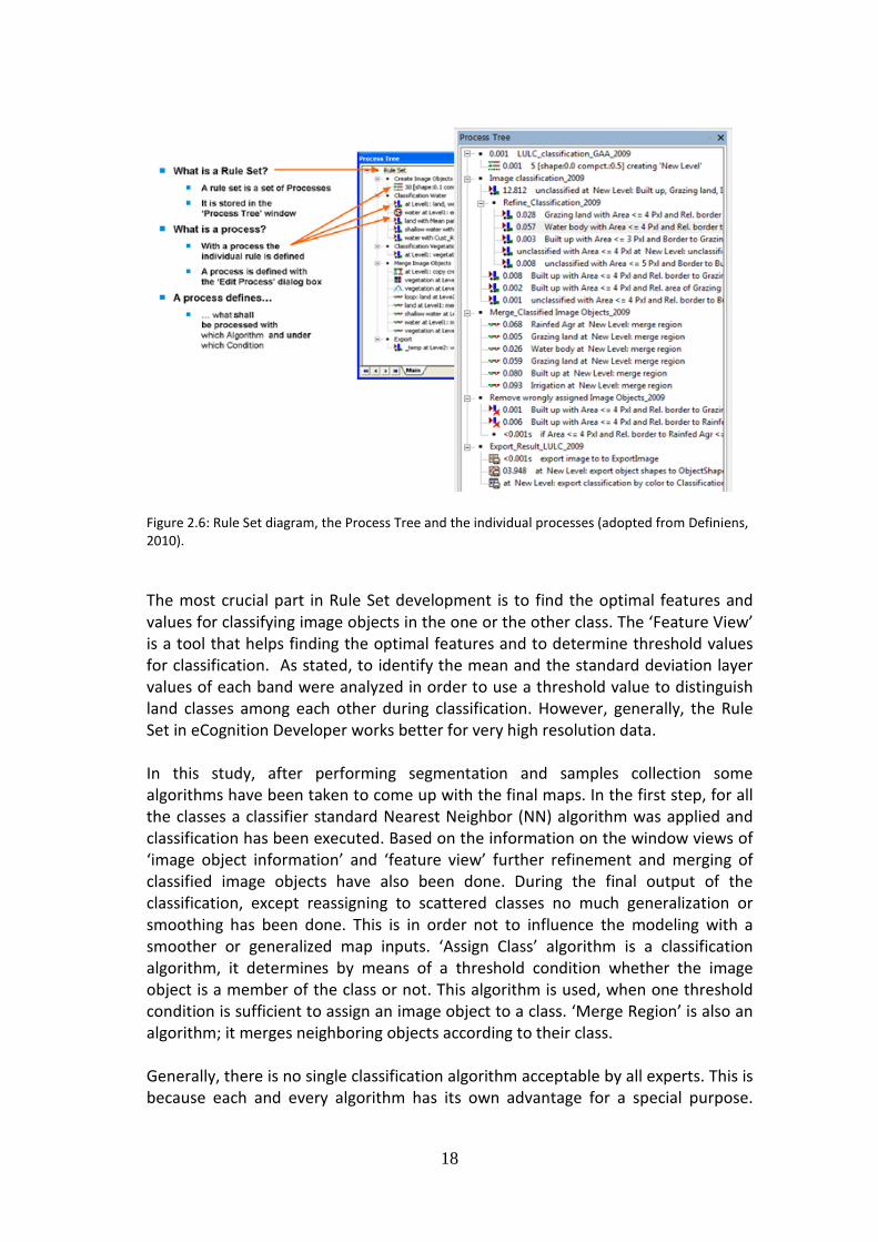
2.3.4 Classification algorithm eCognition works with image objects. The image pixels are grouped together, and as a result much more information is available. Information like the spectral signature of the whole object, the shape and size and also context information is available. All these attributes can be used and combined for classification. In eCognition Definiens, there is no straight forward algorithm to click and perform classification. It is done by writing a rule set. A rule set is a set of processes stored in the “process tree” window (Definiens, 2010). In order to write a rule set, it is necessary to distinguish the information of image objects. Based on that develop a strategy, and then translate the strategy into process of know as Rule Set. The most important tool for creating a Rule Set is the expert knowledge, and the ability to translate the recognition process into the eCognition language. Part of the rule set developed for the year 2009 is shown in the right side of Figure 2.6. Developing a Rule Set does not require to write any code, rather selects from a set of predefined algorithms within the graphical user-interface (Definiens, 2010).

18

Figure 2.6: Rule Set diagram, the Process Tree and the individual processes (adopted from Definiens, 2010). The most crucial part in Rule Set development is to find the optimal features and values for classifying image objects in the one or the other class. The ‘Feature View’ is a tool that helps finding the optimal features and to determine threshold values for classification. As stated, to identify the mean and the standard deviation layer values of each band were analyzed in order to use a threshold value to distinguish land classes among each other during classification. However, generally, the Rule Set in eCognition Developer works better for very high resolution data. In this study, after performing segmentation and samples collection some algorithms have been taken to come up with the final maps. In the first step, for all the classes a classifier standard Nearest Neighbor (NN) algorithm was applied and classification has been executed. Based on the information on the window views of ‘image object information’ and ‘feature view’ further refinement and merging of classified image objects have also been done. During the final output of the classification, except reassigning to scattered classes no much generalization or smoothing has been done. This is in order not to influence the modeling with a smoother or generalized map inputs. ‘Assign Class’ algorithm is a classification algorithm, it determines by means of a threshold condition whether the image object is a member of the class or not. This algorithm is used, when one threshold condition is sufficient to assign an image object to a class. ‘Merge Region’ is also an algorithm; it merges neighboring objects according to their class. Generally, there is no single classification algorithm acceptable by all experts. This is because each and every algorithm has its own advantage for a special purpose.

19

Hence, the understanding of the classification algorithm to be applied is important. All types of classification can be categorized into supervised and unsupervised. Supervised classification has been widely used in remote sensing applications (Yuksel et al., 2008). In this study, supervised classification with the standard NN has been applied for all the classes. It is a sample-based user-defined classification algorithm. Based on samples, a nearest neighbor algorithm combined with predefined feature sets is used to assign objects to classes (Definiens, 2009). The Nearest Neighbor classifier is recommended for a heterogeneous combination of object features like urban areas. The principle is simple first; the algorithm needs samples that are typical representatives for each class. Based on these samples, it searches for the closest sample image object in the feature space of each image object. If an image object's closest sample object belongs to a certain class, the image object will be assigned to it. 2.4: Classification results and validation

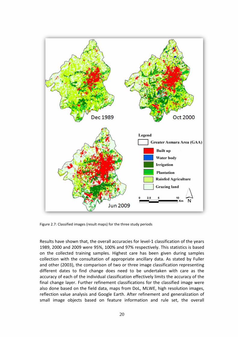
2.4.1 Landuse maps Object based image classification in eCognition stand on the concept that interpretation of an image is not only based on a single pixel attribute rather on the attributes of groups of pixels (image objects). Hence, object based classifier can deliver better results than conventional methods and directs to higher classification accuracy. In this study, the reference maps (Figure 2.7) have been used to understand the attribute of the image objects in order to collect training samples for classification.

2.4.2 Classification validation Landuse landcover maps derived from classification of images usually contain some sort of errors due to several factors that range from classification techniques to methods of satellite data capture. Hence, validation of classification results is an important process in the classification procedure. It allows users to evaluate the utility of a thematic map for their intended applications. For the three classified images, the errors were evaluated and quantified in terms of classification accuracy tool available in eCognition (Table 2.4). eCognition Developer use accuracy assessment methods to produce statistical outputs which can be used to check the quality of the classification results. This is based on an error matrix (also known as confusion matrix) which compares on class-by-class based on the training samples and classification.

20

Figure 2.7: Classified images (result maps) for the three study periods Results have shown that, the overall accuracies for level-1 classification of the years 1989, 2000 and 2009 were 95%, 100% and 97% respectively. This statistics is based on the collected training samples. Highest care has been given during samples collection with the consultation of appropriate ancillary data. As stated by Fuller and other (2003), the comparison of two or three image classification representing different dates to find change does need to be undertaken with care as the accuracy of each of the individual classification effectively limits the accuracy of the final change layer. Further refinement classifications for the classified image were also done based on the field data, maps from DoL, MLWE, high resolution images, reflection value analysis and Google Earth. After refinement and generalization of small image objects based on feature information and rule set, the overall

21

accuracies results have decreased to 94.6% and 94.5% for the year 2000 and 2009 respectively. eCognition also computes the Kappa Index of Agreement (KIA) and similarly, after refinement classification, KIA (Congalton, 1999) has also decreased from 97 % to 94% for the year 1989, from100% to 93% for the year 2000; and from 95.8% to 91.8% for 2009. The further classification refinements performed were reassigning of scattered pixels and merging of small pixels inside bigger class. These were only for image objects less than four pixels size. Otherwise, no smoothing and generalization of pixels have done, this is, in order not to influence the change detection and modeling processes. Detailed classification refinement could not be done for the year 1989 because of the shortage of ancillary data.

Producer's User's KIA per Class Land Class 1989 2000 2009 1989 2000 2009 1989 2000 2009 Built up 1 1 0.98 1 1 1 1 1 0.97 Irrigation 1 1 1 0.71 1 0.68 1 1 1 Raifed Agri. 0.95 0.8 0.9 0.95 1 0.66 0.93 0.74 0.9 Plantation 0.88 1 0.85 1 0.8 1 0.87 1 0.85 Water body 1 1 1 1 1 1 1 1 1 Grazing land 0.88 1 0.91 1 1 1 0.87 1 0.85 Map of: 1989 2000 2009 Overall accuracy 0.952 0.946 0.945 KIA 0.937 0.934 0.918

Table 2.4: Summary of error matrixes for the classified images of 1989, 2000 and 2009 Furthermore, the analyst tried to compare the sample based accuracy result in eCognition with secondary data (that is, based on a reference map). The comparison was done by generating 200 stratified random points from the classified image of 2009 in ArcMap. These points were verified and labeled against the reference map for the year 2007 obtained from DoL, MLWE. The classified image MMU corresponds to four image pixels (3600m2

), whereas, the reference map has not standard MMU and the analyst made use of Google Erath for further verification. Built up, Water body, Irrigation and Plantation were easily distinguishable, but not for Raifed and Grazing land classes. As stated by (Congalton, 1991), the overall, user‘s and producer‘s accuracies were calculated from the matrices in Table 2.5.

22

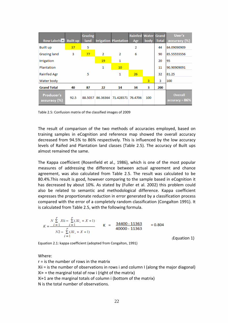
Table 2.5: Confusion matrix of the classified images of 2009

The result of comparison of the two methods of accuracies employed, based on training samples in eCognition and reference map showed the overall accuracy decreased from 94.5% to 86% respectively. This is influenced by the low accuracy levels of Raifed and Plantation land classes (Table 2.5). The accuracy of Built ups almost remained the same. The Kappa coefficient (Rosenfield et al., 1986), which is one of the most popular measures of addressing the difference between actual agreement and chance agreement, was also calculated from Table 2.5. The result was calculated to be 80.4%.This result is good, however comparing to the sample based in eCognition it has decreased by about 10%. As stated by (Fuller et al. 2002) this problem could also be related to semantic and methodological difference. Kappa coefficient expresses the proportionate reduction in error generated by a classification process compared with the error of a completely random classification (Congalton 1991). It is calculated from Table 2.5, with the following formula.

(Equation 1)

Equation 2.1: kappa coefficient (adopted from Congalton, 1991)

Where: r = is the number of rows in the matrix Xii = is the number of observations in rows i and column I (along the major diagonal) Xi+ = the marginal total of row i (right of the matrix) Xi+1 are the marginal totals of column i (bottom of the matrix) N is the total number of observations.

23

From this result the analyst assumes that the two accuracy assessment methods employed are comparable. Hence, the accuracy results calculated in eCognition software for the classified images of 1989 and 2000 are acceptable.

2.5: Results and discussion In this study, ERDAS Imagine 9.2 was used for pre-processing the Landsat TM data, and the images were fine inputs for further analysis and classification. The software chosen for classification was eCognition Definiens 8, it is also known as eCognition Developer, and the produced maps have acceptable level of accuracy for further analysis and modeling. Hence, in such studies although availability is a constraint it is important to identify the strong side of the available software in order to get desirable results. As stated by Araya et al., (2010) object-oriented technique has been suggested for a better and more cohesive classification result. Hence, object-based classification was employed in order to get more accurate results. Though, the obtained accuracy of the image classification from Landsat imagery is to the acceptable level, with Definiens and its functionalities in classification and rule set processes, it is possible to get more accurate maps from high resolution imageries. In this study, during image classification more focus has been given to Built-up areas. In the TM images, the Built-up and Water classes were relatively easily distinguishable from the other classes. Irrigated and Plantation land classes were also identified with the use of the ancillary data. Whereas, the distinction between Raifed agriculture and Grazing land classes special in the year 1989 and 2009 was not simple. Though, reference data for the year 1989 was not available the procedures followed and the algorithms applied were the same for all the three study period. Hence, the accuracy of the classified image of 1989 is assumed the same as the images of 2000 and 2009. In conclusion, the classified images and their accuracy level fulfill the minimum threshold for further processes.

24

CHAPTER THREE

Urban Landuse Change Detection and Urban Sprawl Analysis 3.1: Introduction A considerable number of studies in urban landuse change detection and sprawl measurement with the application of geospatial tools have been done. Among all few are: Remote sensing can be used to acquire spatiotemporal series of geographical data and to perform land use land cover change (LUCC) analysis (Mucher, 2000; Weng, 2002; Heinimann, 2003; Cabral, 2005). The acquired data is processed and analyzed using geographical information system (GIS) and Remote sensing (RS) techniques and useful information can be obtained for environmental and urban growth monitoring (Goodchild, 2000; Masser, 2001; Cheng, 2003). Similarly, Im et al. (2008) has put remote sensing approaches are widely used for change detection analysis; and (Herold et al. 2002) remote sensing have great potential for the acquisition of detailed and accurate surface information for managing and planning urban regions. An overall idea about image classification and validation for the GAA has been provided in Chapter-2. As a continuation, the main purpose of this chapter is: LUCC detection among the six land classes that have been classified in the last chapter. Plus, examine urban sprawling, which of the land classes have expanded and at the expense of which land classes; and analyze the result why certain classes have been expanding while others were shrinking. Specially, the analyst will focus to investigate how the built up areas changed in the study site during the 20 years study periods (1989 to 2009). In order to detect, quantify and analyze the changes post classification change analyses with ArcMap and ‘Land Change Modeler’ in IDRISI Andes have been employed. Moreover, urban sprawl has also been measured and analyzed. Shannon’s Entropy (an urban sprawl index) has been used to measure the urban sprawl in the Greater Asmara Area (GAA). 3.2: Urban land use land cover change (LUCC) detection Change detection is the process of identifying differences in the state of an object or phenomenon by observing it at different times. Essentially, it involves the ability to quantify temporal effects using multi-temporal data sets (Singh, 1989). Various researchers (Belaid 2003; Jensen et al. 2005; Berkavoa 2007) have attempted to group change detection methods into different broad categories based on the data transformation procedures and the analysis of techniques applied. However, numerous techniques are applied on images of different dates in order to detect the changes occurred through the years. Hence, the techniques are generally divided into two categories: pre-classification and post-classification change detection methods. Pre-classification techniques are applied on rectified and normalized corrected images of single band, or could be on many bands of the image

25

(e.g., image algebra, transformations, etc.) and detect the possible position of change without providing any information for the type of land cover change (Ridd and Liu, 1998; Singh, 1989; Yuan, et al., 1998). The pre-classification and change detection methods can be performed in various software platforms. Whereas, post-classification techniques, are based on the comparison of classified images and provide detailed information about the nature of change for every pixel or object (Im et al., 2005). According to Abuelgasim et al., (1999), the pre-classification are known as categorical while post-classification are continuous of changes detection techniques. In this research, after proving image registration of the three images, both the pre and post-classification techniques have been done. The pre-classification change detection was done mainly to have a general understanding of the changed and unchanged areas of the GAA. The pre-classification method used is discussed briefly below, and the post-classification will proceed next.

3.2.1 Pre-classification change detection with image difference Pre-classification change detection technique is also known as pre-classification spectral change (Pilon et al. 1988, Singh 1989); in ERDAS Imagine 9.2 it is known as image difference. Image Difference is the most commonly used change detection algorithm (Singh, 1989). It involves subtracting one date of imagery from a second date that has been accurately registered (Yuan et al, 1996)

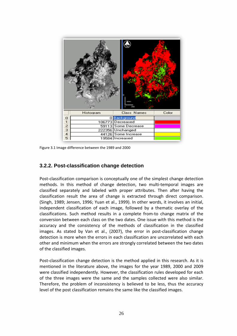
. To compute differences between two images of 1989 versus 2000 and 2000 versus 2009, in both cases the image difference was accomplished in a single band basis (band 7). A threshold value of 10 was given to evaluate the change more than 10% between the images. Since Change Detection calculates change in brightness values over time, the Image Difference File reflects that change using the grayscale image (Figure 3.1). However, there is an option to see a Highlight Change Image. This pre-classification change detection was employed in order to have a general understanding of change, (Figure 3.1) which is a five-class thematic image, typically divided into the five categories of Background, Decreased, Some Decreased, Unchanged, Some Increase, and Increased in the classified image.

26

Figure 3.1 Image difference between the 1989 and 2000

3.2.2. Post-classification change detection Post-classification comparison is conceptually one of the simplest change detection methods. In this method of change detection, two multi-temporal images are classified separately and labeled with proper attributes. Then after having the classification result the area of change is extracted through direct comparison. (Singh, 1989; Jensen, 1996; Yuan et al., 1999). In other words, it

involves an initial, independent classification of each image, followed by a thematic overlay of the classifications. Such method results in a complete from-to change matrix of the conversion between each class on the two dates. One issue with this method is the accuracy and the consistency of the methods of classification in the classified images. As stated by Van et al., (2007), the error in post-classification change detection is more when the errors in each classification are uncorrelated with each other and minimum when the errors are strongly correlated between the two dates of the classified images.

Post-classification change detection is the method applied in this research. As it is mentioned in the literature above, the images for the year 1989, 2000 and 2009 were classified independently. However, the classification rules developed for each of the three images were the same and the samples collected were also similar. Therefore, the problem of inconsistency is believed to be less, thus the accuracy level of the post classification remains the same like the classified images.

27

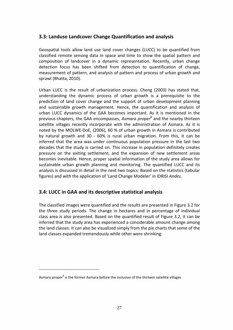
3.3: Landuse Landcover Change Quantification and analysis Geospatial tools allow land use land cover changes (LUCC) to be quantified from classified remote sensing data in space and time to show the spatial pattern and composition of landcover in a dynamic representation.

Recently, urban change detection focus has been shifted from detection to quantification of change, measurement of pattern, and analysis of pattern and process of urban growth and sprawl (Bhatta, 2010).

Urban LUCC is the result of urbanization process. Cheng (2003) has stated that, understanding the dynamic process of urban growth is a prerequisite to the prediction of land cover change and the support of urban development planning and sustainable growth management. Hence, the quantification and analysis of urban LUCC dynamics of the GAA becomes important. As it is mentioned in the previous chapters, the GAA encompasses, Asmara proper8

and the nearby thirteen satellite villages recently incorporate with the administration of Asmara. As it is noted by the MOLWE-DoE, (2006), 60 % of urban growth in Asmara is contributed by natural growth and 30 - 60% is rural urban migration. From this, it can be inferred that the area was under continuous population pressure in the last two decades that the study is carried on. This increase in population definitely creates pressure on the exiting settlement, and the expansion of new settlement areas becomes inevitable. Hence, proper spatial information of the study area allows for sustainable urban growth planning and monitoring. The quantified LUCC and its analysis is discussed in detail in the next two topics: Based on the statistics (tabular figures) and with the application of ‘Land Change Modeler’ in IDRISI Andes.

3.4: LUCC in GAA and its descriptive statistical analysis The classified images were quantified and the results are presented in Figure 3.2 for the thr

ee study periods. The change in hectares and in percentage of individual class area is also presented. Based on the quantified result of Figure 3.2, it can be inferred that the study area has experienced a considerable amount change among the land classes. It can also be visualized simply from the pie charts that some of the land classes expanded tremendously while other were shrinking.

_______________________________ Asmara proper8

is the former Asmara before the inclusion of the thirteen satellite villages

28

NB. The percentage of water body shown in the pie-chart is exaggerated by 60ha in order to be visible.

Figure 3.2: LULC (in hectares) during the three study periods.

In the first decade, from 1989 to 2000, the built up area has increased by about 1700ha, that is more that hundred percent. This could be related with the independence of the country in 1991 that led for a dramatic population boom in the country in general and in the capital city that resulted settlement expansion. An increase in urban population in the post-independence period is associated with different factors including rural-urban migration; returnees from Diaspora, and deportees from Ethiopia (especially after 2000) as well as returnees from Sudan and other countries. These factors trigger the ever-growing demand for urban services: demand of land for residence, economic and industrial activities and other public services. In contrary to built up, the Raifed agricultural area has decreased tremendously, that is about 2800 Raifed

areas were transformed to other land classes. This could be with the change of economic activity of the satellite villages in the GAA. The grazing land and plantation has also decreased while the water body and irrigation increases. The tripling of water body has led for the doubling of Irrigation. This is due to the construction and rehabilitation of dams.

29

As it is stated by Daniel et al., (2009), after the independence of Eritrea, in 1991 about 50 dams have been built in Zoba Maekel9

to promote irrigation and water for domestic use; and most of them are concentrated near Asmara. Moreover, during the attribute data interpretation of the classified images it has also shown that the number of polygons for water body has increased from 79 to 107 from 1989 to 2000 respectively, which proved the increment of dams.

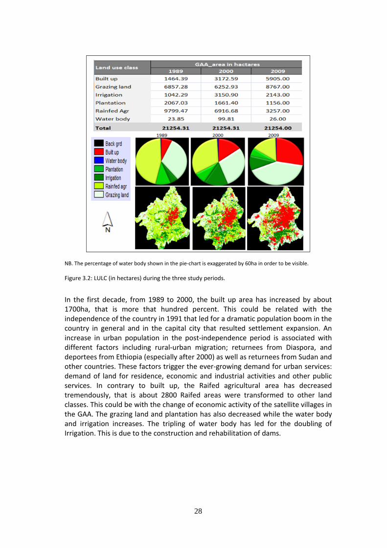
During the second decade (2000 to 2009), the built up area kept the pace of increase and gained more than 2700ha. This indicates that the majority of urban growth is happening beyond the city centre, in surrounding area. Unpredictably, water body and irrigation decreased by about 70% and 30% respectively. Thought it can be inferred that both these land classes have good direct correlation, the dramatic decrease water bodies (mainly dams) was questioned. However, a recent field based study (Daniel et al., (2009)

has proved that due to uncontrolled sedimentation, in the area most of the dams are silted. In Eritrea, in a severe situation of siltation the lifespan of medium and small dams can be less than five years (Negassi et al., (2002). This has also resulted in the decreasing of irrigable areas. More importantly, in the vicinity of Asmara the irrigation lands which are the high potential areas for urban agriculture are severely shrunk due to built up expansion (Figure 3.3).

Figure 3.3: Urban land use conversion, (Source: Google Earth, Nov. 2010)

_____________________________________

Zoba Maekel9 is the central administration zone, where the GAA is the center of that zone

30

Agricultural land is continuously being pushed and converted to urban uses in the process of urbanization. Urban sprawl has been criticized for its inefficient use of land resources and energy and large-scale encroachment on agricultural land (Cheng, 2003). Not only the agricultural areas but also the plantation cover was also decreased, as Rahman et al., (2008) has noted that, the area of urban sprawl is characterized by a situation where urban development negatively interferes with urban setting which is neither an acceptable urban situation nor suitable for an agricultural rural environment. In the last two decades (from 1989 to 2009), the land cover change analysis revealed that built up area has shown a constant increase and finally it tripled. Irrigation and water body has increased in the first decade whereas they decreased in the second decade. Plantation and Raifed agriculture have decreased constantly. Grazing land has decreased in the first decade, but increased in the second decade. This could be associated mainly with two reasons: first, with the expansion of urban area. And second, with incorporation of the satellite villages to the capital city administration, which can lead to change in the economic activities of the villagers. As a result, Raifed agriculture might have abandoned for non agricultural economic activities and classified as grazing land. The above discussion is based on the results obtained from the study; and it is important to note that, though the nomenclature for the land classes used has been developed with the consideration of semantic problems, the land classes used are the generalization of several land classes. For example, Grazing land includes bare soil, barren land and grazing itself. Hence, it is hard to be highly confident if the degree of change shown in the classification reflects the actual change in the land cover of Raifed and grazing which both also have low accuracy assessment. These two classes (Grazing land and Raifed agriculture) are both associated with the same landuse, and it is expected that there is a fluctuation between them according to the patterns of crop seeding, harvesting, and rotation. In addition to that Landsat images used for classification were not captured in the month; there is no surety that the agricultural land was in the same state of use at the time. Given the dynamic variability of these two land cover classes and limited availability of reference map with standard minimum mapping unit (MMU), it does not make sense to draw conclusions with high confidence about the change trends of grazing land and Raifed agriculture areas, apart from the other four land classes which are well referenced. Unlike the two land classes the other four are well distinguished in high resolution images used in the study.

31

Table 3.1: Comparison of LUCC in hectares and in % among the six land classes

In addition to the tabular and pie charts result presented, the analysis has also imported the classified images to Land Change Modeler in IDRISI Andes for further analysis of gains and losses of area among the land classes. Furthermore, with Land Change Modeler, it can be analyzed which land classes have contributed more for the tripling of built up area, which is the main focus of the study.

For the convenience of the reader of this material, the quantified LUCC and their analysis are presented sequentially. The first part (3.5.1) discusses the change from 1989 to 2000, the next part (3.5.2) from 2000 to 2009 and last part (3.5.3) discusses the 20 years change that is from 1989 to 2009.

3.5: LUCC results of the GAA, analysis with Land Change Modeler Landcover change model tools support the analysis of the land use changes. Use of such model also gives a better understanding of the functions of the land use systems and the support needed for planning and policy making. Such models can also predict the possible future change and use of the landcover under different scenario (IDRISI focus paper, 2009). There are many such models available, and for this study Land Change Modeler of IDRISI Andes is used.

Land Change Modeler (LCM), is a suite of tool for land cover change analysis, allows mapping changes in urban land cover changes. Change Analysis with LCM has a set of tools, for the rapid assessment of change, allowing one to evaluations gains and losses, net change, persistence and specific transitions both in map, statistical and graphical form (Eastman, 2006). The change analysis that has been done with LCM for GAA is presented below.

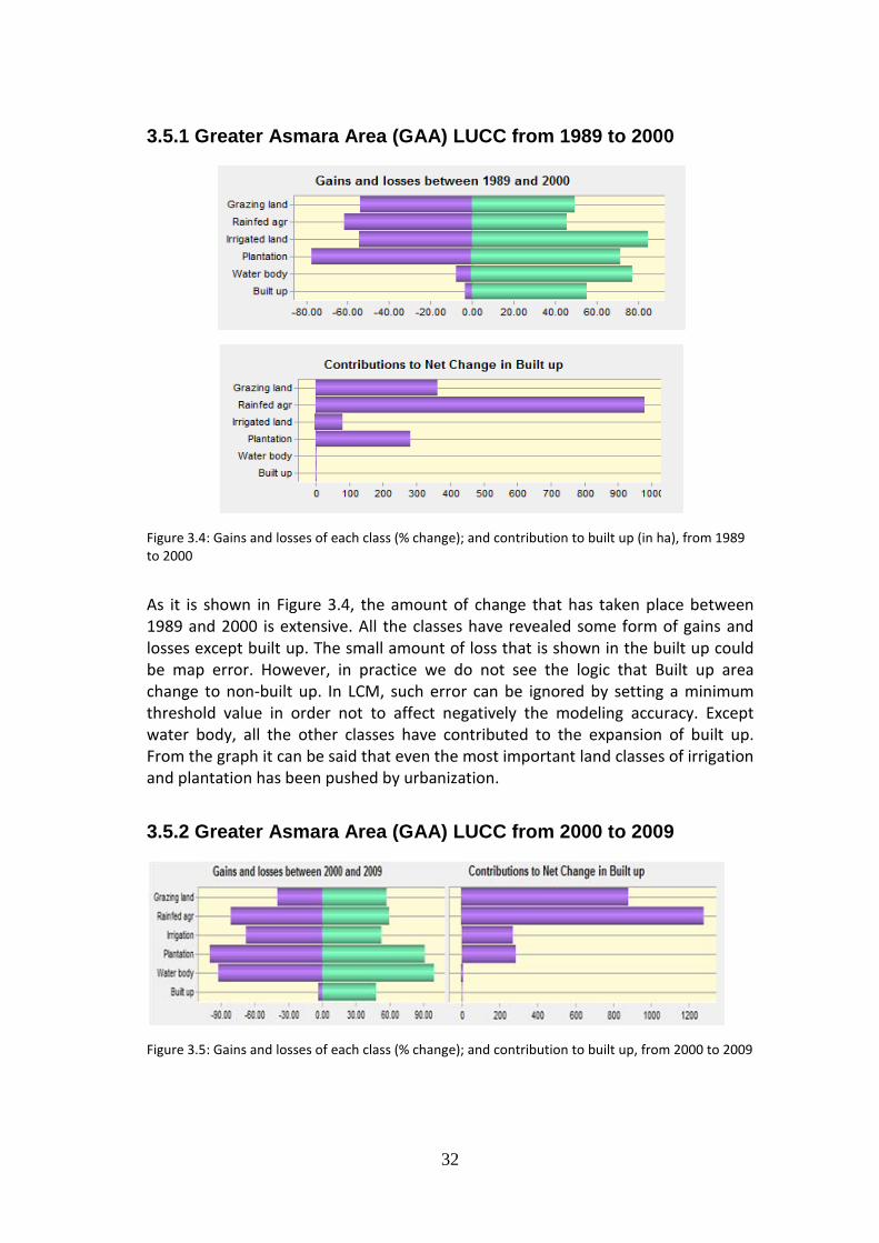
32

3.5.1 Greater Asmara Area (GAA) LUCC from 1989 to 2000

Figure 3.4: Gains and losses of each class (% change); and contribution to built up (in ha), from 1989 to 2000

As it is shown in Figure 3.4, the amount of change that has taken place between 1989 and 2000 is extensive. All the classes have revealed some form of gains and losses except built up. The small amount of loss that is shown in the built up could be map error. However, in practice we do not see the logic that Built up area change to non-built up. In LCM, such error can be ignored by setting a minimum threshold value in order not to affect negatively the modeling accuracy. Except water body, all the other classes have contributed to the expansion of built up. From the graph it can be said that even the most important land classes of irrigation and plantation has been pushed by urbanization.

3.5.2 Greater Asmara Area (GAA) LUCC from 2000 to 2009

Figure 3.5: Gains and losses of each class (% change); and contribution to built up, from 2000 to 2009

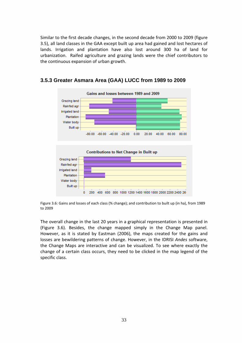
33

Similar to the first decade changes, in the second decade from 2000 to 2009 (figure 3.5), all land classes in the GAA except built up area had gained and lost hectares of lands. Irrigation and plantation have also lost around 300 ha of land for urbanization. Raifed agriculture and grazing lands were the chief contributors to the continuous expansion of urban growth.

3.5.3 Greater Asmara Area (GAA) LUCC from 1989 to 2009

Figure 3.6: Gains and losses of each class (% change); and contribution to built up (in ha), from 1989 to 2009

The overall change in the last 20 years in a graphical representation is presented in (Figure 3.6). Besides, the change mapped simply in the Change Map panel. However, as it is stated by Eastman (2006), the maps created for the gains and losses are bewildering patterns of change. However, in the IDRISI Andes software, the Change Maps are interactive and can be visualized. To see where exactly the change of a certain class occurs, they need to be clicked in the map legend of the specific class.

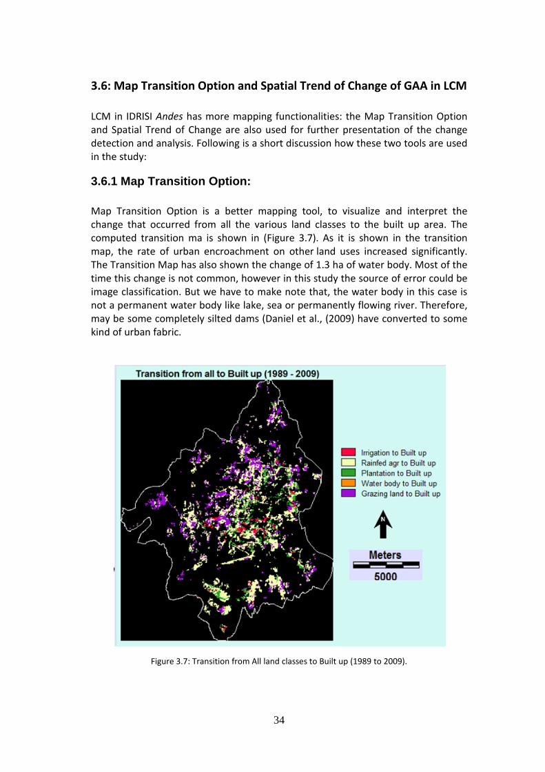
34

3.6: Map Transition Option and Spatial Trend of Change of GAA in LCM LCM in IDRISI Andes has more mapping functionalities: the Map Transition Option and Spatial Trend of Change are also used for further presentation of the change detection and analysis. Following is a short discussion how these two tools are used in the study:

3.6.1 Map Transition Option: Map Transition Option is a better mapping tool, to visualize and interpret the change that occurred from all the various land classes to the built up area. The computed transition ma is shown in (Figure 3.7). As it is shown in the transition map, the rate of urban encroachment on other land uses increased significantly. The Transition Map has also shown the change of 1.3 ha of water body. Most of the time this change is not common, however in this study the source of error could be image classification. But we have to make note that, the water body in this case is not a permanent water body like lake, sea or permanently flowing river. Therefore, may be some completely silted dams (Daniel et al., (2009)

have converted to some kind of urban fabric.

Figure 3.7: Transition from All land classes to Built up (1989 to 2009).

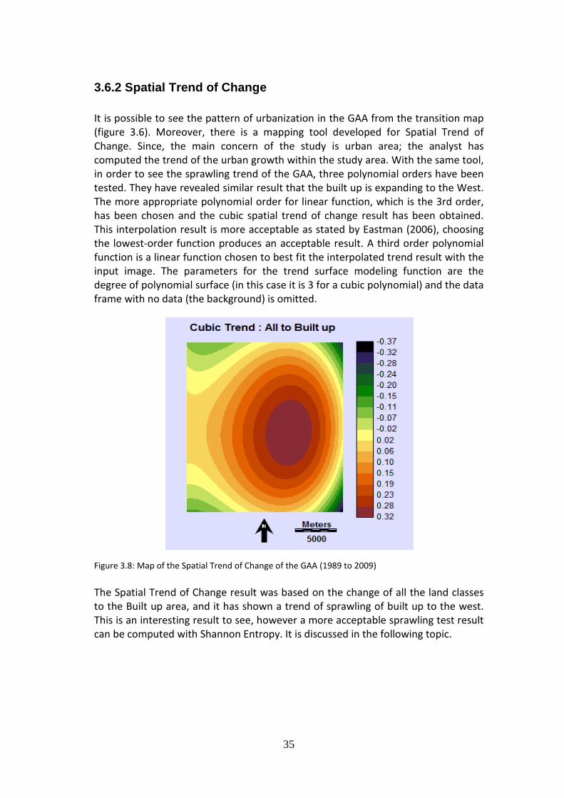
35

3.6.2 Spatial Trend of Change It is possible to see the pattern of urbanization in the GAA from the transition map (figure 3.6). Moreover, there is a mapping tool developed for Spatial Trend of Change. Since, the main concern of the study is urban area; the analyst has computed the trend of the urban growth within the study area. With the same tool, in order to see the sprawling trend of the GAA, three polynomial orders have been tested. They have revealed similar result that the built up is expanding to the West. The more appropriate polynomial order for linear function, which is the 3rd order, has been chosen and the cubic spatial trend of change result has been obtained. This interpolation result is more acceptable as stated by Eastman (2006), choosing the lowest-order function produces an acceptable result. A third order polynomial function is a linear function chosen to best fit the interpolated trend result with the input image. The parameters for the trend surface modeling function are the degree of polynomial surface (in this case it is 3 for a cubic polynomial) and the data frame with no data (the background) is omitted.

Figure 3.8: Map of the Spatial Trend of Change of the GAA (1989 to 2009) The Spatial Trend of Change result was based on the change of all the land classes to the Built up area, and it has shown a trend of sprawling of built up to the west. This is an interesting result to see, however a more acceptable sprawling test result can be computed with Shannon Entropy. It is discussed in the following topic.

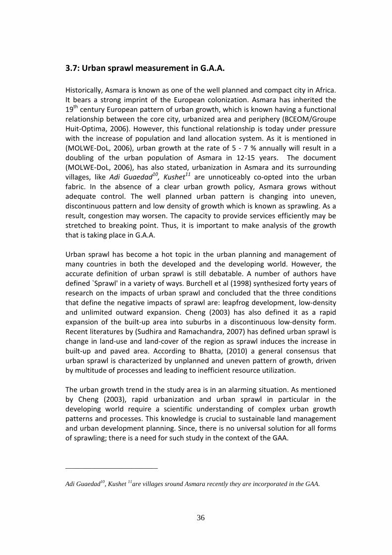
36

3.7: Urban sprawl measurement in G.A.A. Historically, Asmara is known as one of the well planned and compact city in Africa. It bears a strong imprint of the European colonization. Asmara has inherited the 19th century European pattern of urban growth, which is known having a functional relationship between the core city, urbanized area and periphery (BCEOM/Groupe Huit-Optima, 2006). However, this functional relationship is today under pressure with the increase of population and land allocation system. As it is mentioned in (MOLWE-DoL, 2006), urban growth at the rate of 5 - 7 % annually will result in a doubling of the urban population of Asmara in 12-15 years. The document (MOLWE-DoL, 2006), has also stated, urbanization in Asmara and its surrounding villages, like Adi Guaedad10, Kushet11

are unnoticeably co-opted into the urban fabric. In the absence of a clear urban growth policy, Asmara grows without adequate control. The well planned urban pattern is changing into uneven, discontinuous pattern and low density of growth which is known as sprawling. As a result, congestion may worsen. The capacity to provide services efficiently may be stretched to breaking point. Thus, it is important to make analysis of the growth that is taking place in G.A.A.

Urban sprawl has become a hot topic in the urban planning and management of many countries in both the developed and the developing world. However, the accurate definition of urban sprawl is still debatable. A number of authors have defined `Sprawl' in a variety of ways. Burchell et al (1998) synthesized forty years of research on the impacts of urban sprawl and concluded that the three conditions that define the negative impacts of sprawl are: leapfrog development, low-density and unlimited outward expansion. Cheng (2003) has also defined it as a rapid expansion of the built-up area into suburbs in a discontinuous low-density form. Recent literatures by (Sudhira and Ramachandra, 2007) has defined urban sprawl is change in land-use and land-cover of the region as sprawl induces the increase in built-up and paved area. According to Bhatta, (2010) a general consensus that urban sprawl is characterized by unplanned and uneven pattern of growth, driven by multitude of processes and leading to inefficient resource utilization. The urban growth trend in the study area is in an alarming situation. As mentioned by Cheng (2003), rapid urbanization and urban sprawl in particular in the developing world require a scientific understanding of complex urban growth patterns and processes. This knowledge is crucial to sustainable land management and urban development planning. Since, there is no universal solution for all forms of sprawling; there is a need for such study in the context of the GAA. ____________________________

Adi Guaedad10, Kushet 11are villages sround Asmara recently they are incorporated in the GAA.

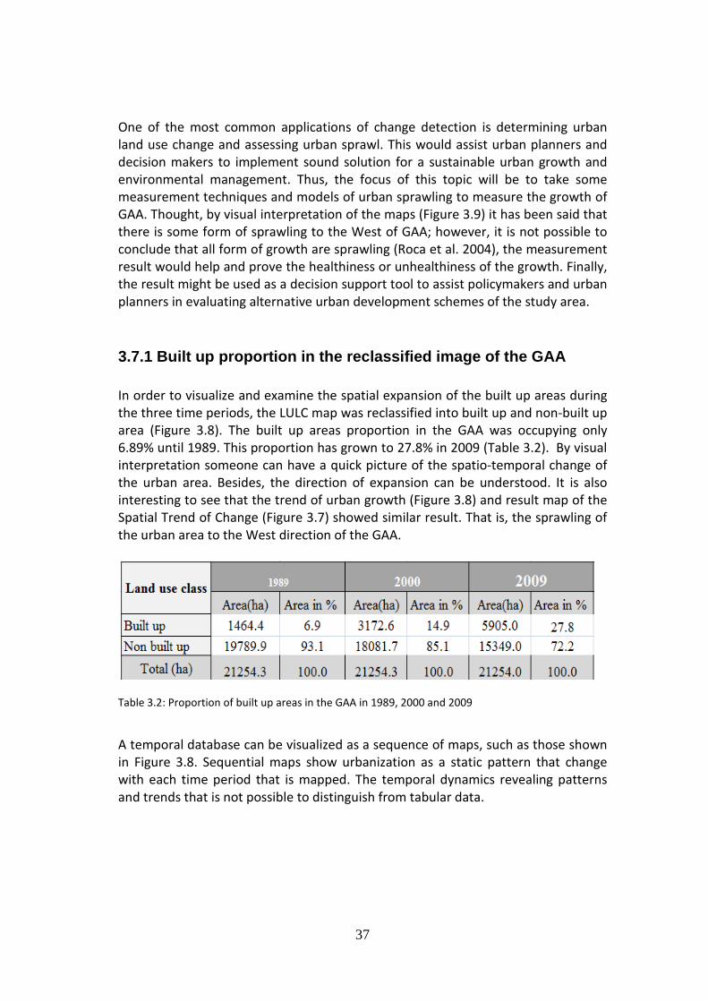
37

One of the most common applications of change detection is determining urban land use change and assessing urban sprawl. This would assist urban planners and decision makers to implement sound solution for a sustainable urban growth and environmental management. Thus, the focus of this topic will be to take some measurement techniques and models of urban sprawling to measure the growth of GAA. Thought, by visual interpretation of the maps (Figure 3.9) it has been said that there is some form of sprawling to the West of GAA; however, it is not possible to conclude that all form of growth are sprawling (Roca et al. 2004), the measurement result would help and prove the healthiness or unhealthiness of the growth. Finally, the result might be used as a decision support tool to assist policymakers and urban planners in evaluating alternative urban development schemes of the study area.

3.7.1 Built up proportion in the reclassified image of the GAA In order to visualize and examine the spatial expansion of the built up areas during the three time periods, the LULC map was reclassified into built up and non-built up area (Figure 3.8). The built up areas proportion in the GAA was occupying only 6.89% until 1989. This proportion has grown to 27.8% in 2009 (Table 3.2). By visual interpretation someone can have a quick picture of the spatio-temporal change of the urban area. Besides, the direction of expansion can be understood. It is also interesting to see that the trend of urban growth (Figure 3.8) and result map of the Spatial Trend of Change (Figure 3.7) showed similar result. That is, the sprawling of the urban area to the West direction of the GAA.

Table 3.2: Proportion of built up areas in the GAA in 1989, 2000 and 2009

A temporal database can be visualized as a sequence of maps, such as those shown in Figure 3.8. Sequential maps show urbanization as a static pattern that change with each time period that is mapped. The temporal dynamics revealing patterns and trends that is not possible to distinguish from tabular data.

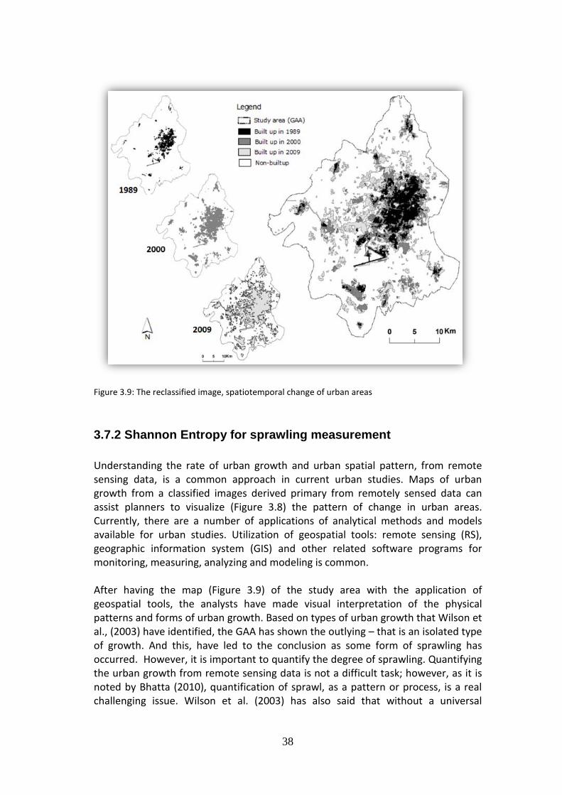
38

Figure 3.9: The reclassified image, spatiotemporal change of urban areas

3.7.2 Shannon Entropy for sprawling measurement Understanding the rate of urban growth and urban spatial pattern, from remote sensing data, is a common approach in current urban studies. Maps of urban growth from a classified images derived primary from remotely sensed data can assist planners to visualize (Figure 3.8) the pattern of change in urban areas. Currently, there are a number of applications of analytical methods and models available for urban studies. Utilization of geospatial tools: remote sensing (RS), geographic information system (GIS) and other related software programs for monitoring, measuring, analyzing and modeling is common. After having the map (Figure 3.9) of the study area with the application of geospatial tools, the analysts have made visual interpretation of the physical patterns and forms of urban growth. Based on types of urban growth that Wilson et al., (2003) have identified, the GAA has shown the outlying – that is an isolated type of growth. And this, have led to the conclusion as some form of sprawling has occurred. However, it is important to quantify the degree of sprawling. Quantifying the urban growth from remote sensing data is not a difficult task; however, as it is noted by Bhatta (2010), quantification of sprawl, as a pattern or process, is a real challenging issue. Wilson et al. (2003) has also said that without a universal

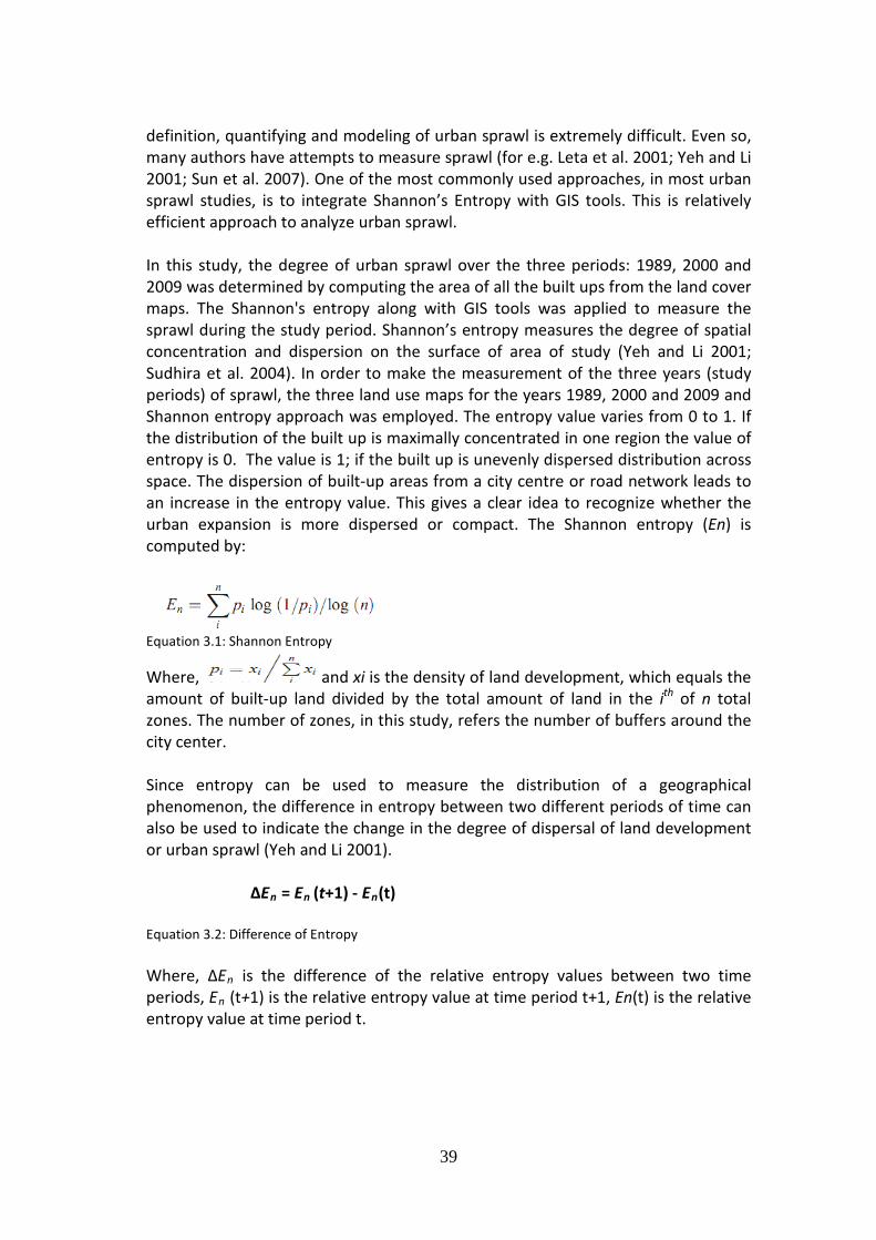
39

definition, quantifying and modeling of urban sprawl is extremely difficult. Even so, many authors have attempts to measure sprawl (for e.g. Leta et al. 2001; Yeh and Li 2001; Sun et al. 2007). One of the most commonly used approaches, in most urban sprawl studies, is to integrate Shannon’s Entropy with GIS tools. This is relatively efficient approach to analyze urban sprawl. In this study, the degree of urban sprawl over the three periods: 1989, 2000 and 2009 was determined by computing the area of all the built ups from the land cover maps. The Shannon's entropy along with GIS tools was applied to measure the sprawl during the study period. Shannon’s entropy measures the degree of spatial concentration and dispersion on the surface of area of study (Yeh and Li 2001; Sudhira et al. 2004). In order to make the measurement of the three years (study periods) of sprawl, the three land use maps for the years 1989, 2000 and 2009 and Shannon entropy approach was employed. The entropy value varies from 0 to 1. If the distribution of the built up is maximally concentrated in one region the value of entropy is 0. The value is 1; if the built up is unevenly dispersed distribution across space. The dispersion of built-up areas from a city centre or road network leads to an increase in the entropy value. This gives a clear idea to recognize whether the urban expansion is more dispersed or compact. The Shannon entropy (En) is computed by:

Equation 3.1: Shannon Entropy

Where, and xi is the density of land development, which equals the amount of built-up land divided by the total amount of land in the ith

of n total zones. The number of zones, in this study, refers the number of buffers around the city center.

Since entropy can be used to measure the distribution of a geographical phenomenon, the difference in entropy between two different periods of time can also be used to indicate the change in the degree of dispersal of land development or urban sprawl (Yeh and Li 2001).

ΔEn = En (t+1) - En

(t)

Equation 3.2: Difference of Entropy

Where, ΔEn is the difference of the relative entropy values between two time periods, En

(t+1) is the relative entropy value at time period t+1, En(t) is the relative entropy value at time period t.

40

The following procedures and considerations have been taken to compute the entropy: The three LULC images for the year 1989, 2000 and 2009 have been

reclassified in the built up and non-built up. This is because the main concern is to measure the sprawling of urban (the built up) areas.

The Municipality Office, that is located in the downtown of Asmara has been taken as a city center

For the three time periods 6, 9 and 13 concentric rings, with 1km buffer in between the rings have been generated in ArcMap for the three study periods. Concentric circles have been taken based on the outermost built up area in the three time periods.

For time-1 and time-2, the areas of the satellite villages were not included in computing the density of built up area.

The entropy was calculated using the equations 3.1 and 3.2. Discussion of the result of the sprawling in GAA is presented in the next section.

3.7.3 Urban sprawl in the GAA The entropy of the urban areas in 1989, 2000 and 2009 has been computed. The results obtained for the three study periods are 0.39, 0.42, and 0.97 respectively (Table 3.3). The entropy values indicates that there was less sprawl in the year 1989 and it stated to increase in 2000 and substantial internal variation in the patterns of urban growth has been measured in 2009. Asmara proper is known to be more compacted. The result is showing some degree sprawl, this is due to the North South elongated shape of Asmara proper. In general, urban sprawl was increasing throughout the study periods because of the fragmented type of growth. It is found that fragmentation of land use causes loss of environmentally fragile lands, loss of farmland as well as economic cost of urban growth (Buiton, 1994; Johnson, 2001). The measurement of the difference on entropy between (t) and (t+1) was also computed, using Equation 3.2 to indicate the temporal change in the degree of dispersal of land development or urban sprawl. The change in the entropy values is given in Table 3.3.

En ΔE (entropy during the 3 study

periods) n (Difference of entropy)

1989 2000 2009 1989 - 2000 2000 - 2009 1989 -2009

0.3927 0.4288 0.9795 0.0361 0.5507 0.5868

Table 3.3: Shannon’s Entropy values of the three years and difference among the periods

41

Figure 3.10: Graph of the entropy value of GAA (1989, 2000 and 2009)

The entropy value from 2000 to 2009 has increased rapidly (Figure 3.10). This indicates a large amount of sprawl of built up area in the GAA. However, it is also important to consider that the incorporation of the thirteen satellite villages during sprawl computation has made an increase of areas of less developed between Asmara proper and the villages. This might have further pushed the sprawl value. 3.8: Discussion In this chapter, the main steps accomplished are summarized briefly. These are: LUCC detection, quantification and analysis for the three classified images of the 1989, 2000 and 2009 with descriptive statistics have been performed. LCM in IDRISI Andes has also been used for analysis by graphical representations and in map forms for the LUCC quantification and comparison. Furthermore, LCM was employed to evaluate the transition among all the classes and the transition of all classes to urban areas. After making such analysis, since, the main concern is in urban growth, the LULC was reclassified into built up and non-built up and further analysis has been performed. Urban growth and its trend of change was evaluated; comparison of the growth between the two decade (1989 to 2000 and 2000 to 2009), plus from 1989 to 2009 has been done. Finally, the urban sprawl has been measured with Shannon’s Entropy to evaluate how healthy or unhealthy the growth was. As it is mentioned in literatures of urban studies, urban change detection involves the application of multi-temporal datasets to quantify, analyze the temporal effects of the phenomenon (Lu et al. 2004). Various techniques have been developed to improve change detection accuracy, including image differencing, image rationing, post classification comparison, etc. However, no single change detection approach can globally be recommended. In this study, post classification comparison which is the most popular method of urban change detection is employed (Jensen et al. 1993). Change detection and quantifying the urban growth from remote sensing data and was not a difficult task; however, quantification of sprawl, as a pattern or process, was a challenging (Bhatta, 2010). LCM in IDRISI has a set of tools for

42

assessment of change, evaluation of gains and losses, net change, transitions both in map and graphical form (IDRISI focus paper, 2009). In some situations, the amount and nature of change can be very complex. However, LCM includes a change abstraction tool, based on trend surface analysis, to uncover the underlying trends. Entropy sprawl measurement is the most widely used technique to measure the extent of urban sprawl with the integration of remote sensing data and GIS (Yeh and Li 2001a; Lata et al. 2001; Li and Yeh 2004; Sudhira et al., 2004; Bhatta et al. 2010a). The LUCC detection presented in this chapter has allowed for the identification of land cover change trends, with respect to six major land cover classes: built up, grazing land, irrigation, plantation, Raifed agriculture and water body. The focus of the change detection and analysis has been on assessing the transitions among the land classes in relation to the growth of urban areas within the GAA. The land cover change analysis revealed that in the last two decades, the urban area has tripled in size. However, this growth was measured, and the degree of sprawling obtained from the Entropy value has indicated it was not healthy. This means, the urban growth has affected the landscape ecology of the GAA negatively. Although, urban sprawl can be seen as economic growth in an area; nevertheless, negative impacts are generally more highlighted because sprawl is often uncontrolled or uncoordinated and therefore the negative impacts override the positive sides’ of urban growth. The causes that force growth in urban areas and the causes that are responsible for undesirable pattern or process of urban growth are also important for the analysis of urban growth. However, remote sensing data are more widely used for the analysis of pattern and process rather than causes and/or consequences. Hence, in-depth studies regarding the causes and consequences are not the purpose of this study. Bhatta (2010) has listed causes of compact urban growth and urban sprawl. According to him the following are some of the causes for undesirable urban growth which might be true in the case of GAA: population growth, independence of decision, physical geography, lack of proper planning policies, government developmental policies failure to enforce planning policies et cetera. Consequences of urban sprawl: inflated infrastructure and public service costs, loss of farmland, disparity in wealth, impacts on water quantity and quality, impacts on public and social health and others. Though this research has not done thoroughly study on the causes of LUCC in the GAA, the major driving forces can be attributed to the following: Population growth: in addition to the normal population growth, after the independence of the country in 1991, population has started to increase at an alarming situation. Moreover, returnees and deportees from Ethiopia as well as returnees from Sudan and other countries have contributed to the population increase in Asmara. According to (UN, 2009) Eritrea had the third highest urban population growth rate in Africa for the years 2000 - 2005, where the annual urban

43

Population growth was 6%. Furthermore, population growth in rural areas resulted migration towards urban areas especially to the capital city Asmara is continuous as occurs elsewhere on the continent. In addition to other pull factors, the moderate climatic condition causes migration. As it is mentioned in FAO (2006), about 65 percent of the population in Eritrea lives in the highlands, which accounts for only 16 percent of the land area. The GAA is located on the central highlands of the country, which has moderate and favorable climate throughout the year. Despite the regional economic importance, the trend of urban growth remains the major factor for diminishing land resources. As stated by Xie et al., (2005), one of the direct consequences of rapid urbanization and population growth is the loss of agricultural land. It is true in the case of GAA. The MOA, (2002) estimated that the ratio between urban population growth rate and urban area growth rate is 0.5, i.e., urban areas grow at one-half the rate of the urban population. Another driving force can be independence of decision as stated by Bhatta (2010) it means, government holds a variety of expectations about the future and a variety of development demands. Often these can take decisions at their own to meet their future expectations and development demands. This is especially true if there is not master plan or if the master plan is override as a whole. This independence ultimately results in uncoordinated, uncontrolled and unplanned development. As it is noted in MOA (2002), ‘Article 46 (Sub-articles 1 & 2) of the Land Reform Proclamation (No. 58/1994) states that the Government shall have supreme authority in formulating the country’s land use policy’. It further states that the power provided shall include the authority to determine the classification of land and its usage and to limit the amount of land to be distributed amongst the usufructuaries. In the year 2004/2005, planned land allocation for Tessa2 (land for housing) and BOND3

(special lease land) was remarkably high, which is over 2500ha for urban development (Housing/Urban Development Policy Report, 2005). From this it can be inferred that the land in the GAA is in pressure and conflict between agricultural and human settlement interests.

In addition to the points mentioned above, some of specific urban sprawling consequences in the GAA are: the loss of land in subsistence agriculture which can be seen as equal to the loss of livelihood. Loss of urban agriculture and food insecurity becomes more acute especially for the urban poor people. It destroys self-reliant agricultural subsistence livelihoods, without necessarily replacing them with any alternative economic activity (MOA, 2002). The trend of urban growth, particularly the expansion of residential and commercial land use, is towards the urban rural fringe, which is normally the agricultural area. It could be seen that such trend of urban growth has been one of the most widespread anthropogenic causes of the loss of arable land, habitat destruction, the decline in natural vegetation cover. The study of urban change detection and change analysis is important. This result may ultimately assist policymakers and

44

decision makers in creating and implementing specific policies to ameliorate undesirable impacts of sprawl or prevent those impacts from occurring. The next chapter discussed on the future trends of land cover change in the study area.

45

CHAPTER FOUR

Modeling Urban Growth Patterns 4.1: Introduction In the previous chapter, the dynamic process of urban growth in GAA was presented. This is a prerequisite to the prediction of land cover change (Cheng, 2003). This chapter discusses about modeling. In general, modeling means the process of creating a representation of reality; it could be a map, graph, picture, or mathematical representation. The focus of this chapter is on spatial modeling, and it discusses on the data used, data processing for modeling, methodology followed, modeling results and validation and, lastly, the discussion about the model results. “A model is an abstraction of an object, system or process that permits knowledge to be gained about reality by conducting experiments on the model” Clark (2003). In this study, land use and land cover change (LUCC) modeling is defined as the process of creating maps based on the history of LUCC, existing information and assumptions of the future. Modeling of LUCC plays a significant role to understand impacts of the changes that occur through time. This would help for effective environmental management, sustainable resources utilization, development plans and decision making. This has become more efficient with the advancement of geospatial tools which provide us the capability to integrate and processed spatial data and various other modeling factors. A number of authors in the field of urban studies have stated several modeling advantages. Pontius et al., (2006) have mentioned that, in the field of urban planning, modeling can be used for analyzing, evaluating, forecasting and simulating urban systems to support decision making. Urban LUCC detection, analysis and modeling plays vital role in planning a healthy growth of urban ecosystem. Ineffectively planned urban growth ends up breaking the equilibrium of environmentally sensitive areas. Scientific models addressing location and quantity of urban expansion in space and time are essential in providing scientists and policy makers with empirical/statistical support for their decisions toward an environmentally sustainable future (Lee et al. 1999). The aim of modeling for Cheng (2003) is to conceptualize and represent the entity being studied. While for Agarwal et al., (2000), the aims of land use land cover modelling is quantitatively specifying the processes of the physical and functional transitions of the land structure and system; and interpret the causal effects hidden in its processes. Similarly, in this study, the LUCC modeling for the GAA is the creation of the representation or abstraction of the future land cover changes that can be quantified, analysed and interpreted to discover the unseen changes and impacts.

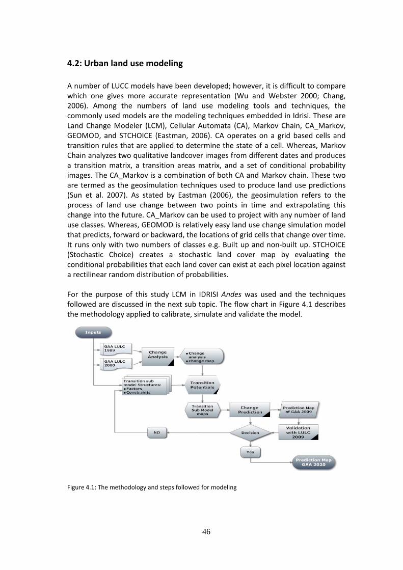
46

4.2: Urban land use modeling A number of LUCC models have been developed; however, it is difficult to compare which one gives more accurate representation (Wu and Webster 2000; Chang, 2006). Among the numbers of land use modeling tools and techniques, the commonly used models are the modeling techniques embedded in Idrisi. These are Land Change Modeler (LCM), Cellular Automata (CA), Markov Chain, CA_Markov, GEOMOD, and STCHOICE (Eastman, 2006). CA operates on a grid based cells and transition rules that are applied to determine the state of a cell. Whereas, Markov Chain analyzes two qualitative landcover images from different dates and produces a transition matrix, a transition areas matrix, and a set of conditional probability images. The CA_Markov is a combination of both CA and Markov chain. These two are termed as the geosimulation techniques used to produce land use predictions (Sun et al. 2007). As stated by Eastman (2006), the geosimulation refers to the process of land use change between two points in time and extrapolating this change into the future. CA_Markov can be used to project with any number of land use classes. Whereas, GEOMOD is relatively easy land use change simulation model that predicts, forward or backward, the locations of grid cells that change over time. It runs only with two numbers of classes e.g. Built up and non-built up. STCHOICE (Stochastic Choice) creates a stochastic land cover map by evaluating the conditional probabilities that each land cover can exist at each pixel location against a rectilinear random distribution of probabilities. For the purpose of this study

LCM in IDRISI Andes was used and the techniques followed are discussed in the next sub topic. The flow chart in Figure 4.1 describes the methodology applied to calibrate, simulate and validate the model.

Figure 4.1: The methodology and steps followed for modeling

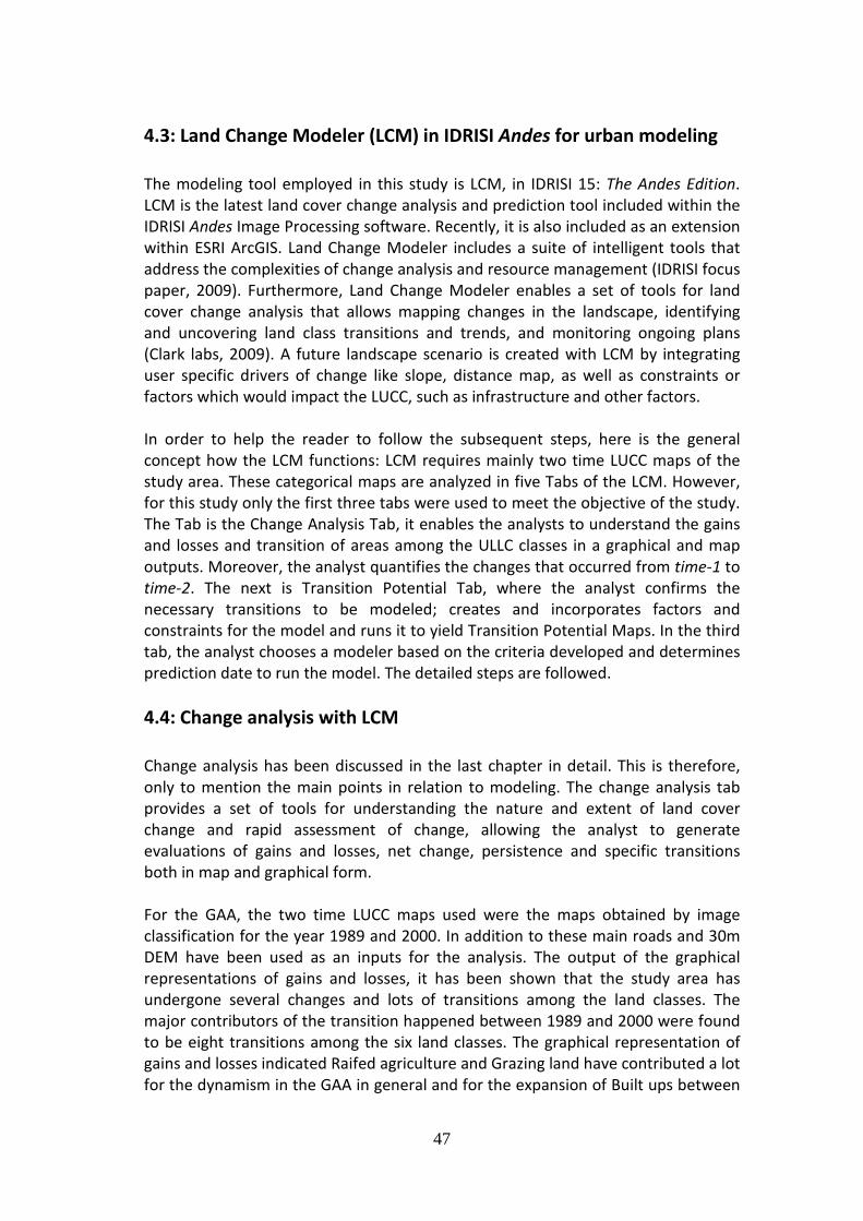
47

4.3: Land Change Modeler (LCM) in IDRISI Andes for urban modeling The modeling tool employed in this study is LCM, in IDRISI 15: The Andes Edition. LCM is the latest land cover change analysis and prediction tool included within the IDRISI Andes Image Processing software. Recently, it is also included as an extension within ESRI ArcGIS. Land Change Modeler includes a suite of intelligent tools that address the complexities of change analysis and resource management (IDRISI focus paper, 2009). Furthermore, Land Change Modeler enables a set of tools for land cover change analysis that allows mapping changes in the landscape, identifying and uncovering land class transitions and trends, and monitoring ongoing plans (Clark labs, 2009). A future landscape scenario is created with LCM by integrating user specific drivers of change like slope, distance map, as well as constraints or factors which would impact the LUCC, such as infrastructure and other factors. In order to help the reader to follow the subsequent steps, here is the general concept how the LCM functions: LCM requires mainly two time LUCC maps of the study area. These categorical maps are analyzed in five Tabs of the LCM. However, for this study only the first three tabs were used to meet the objective of the study. The Tab is the Change Analysis Tab, it enables the analysts to understand the gains and losses and transition of areas among the ULLC classes in a graphical and map outputs. Moreover, the analyst quantifies the changes that occurred from time-1 to time-2. The next is Transition Potential Tab, where the analyst confirms the necessary transitions to be modeled; creates and incorporates factors and constraints for the model and runs it to yield Transition Potential Maps. In the third tab, the analyst chooses a modeler based on the criteria developed and determines prediction date to run the model. The detailed steps are followed. 4.4: Change analysis with LCM Change analysis has been discussed in the last chapter in detail. This is therefore, only to mention the main points in relation to modeling. The change analysis tab provides a set of tools for understanding the nature and extent of land cover change and rapid assessment of change, allowing the analyst to generate evaluations of gains and losses, net change, persistence and specific transitions both in map and graphical form. For the GAA, the two time LUCC maps used were the maps obtained by image classification for the year 1989 and 2000. In addition to these main roads and 30m DEM have been used as an inputs for the analysis. The output of the graphical representations of gains and losses, it has been shown that the study area has undergone several changes and lots of transitions among the land classes. The major contributors of the transition happened between 1989 and 2000 were found to be eight transitions among the six land classes. The graphical representation of gains and losses indicated Raifed agriculture and Grazing land have contributed a lot for the dynamism in the GAA in general and for the expansion of Built ups between

48

the two periods. This is true that open lands are most of the time highly dynamic in nature (Eastman, 2006). In the change analysis tab, it is also possible to analyze and map how much land the urban area has taken from each and every of the other land classes (Figure 4.2). The losses of urban land shown in the maps are probably map error since most of the time it is unlikely to happen urban area changes to another type of land class.

Figure 4.2: Gains and losses of built up area between 1989 and 2000.

Change analysis tab, provides a very effective means of generalizing the change and the change trend. Having all these analysis we go to the next tab,

4.5: Transition Potentials Modeling with LCM The main goal of this tab is to create Transition Potential maps with acceptable degree of accuracy to run the ‘actual’ modeling. Hence, the Transition Potentials tab allows us to group transitions into a set of sub-models and to explore the potential power of explanatory variables. Variables can be added to the model either as static or dynamic components (Eastman, 2006). Static variables express

49

aspects of basic suitability for the transition under consideration, and are unchanging over time. Dynamic variables are time-dependent drivers such as proximity to existing development or infrastructure and are recalculated over time during the course of a prediction.

4.5.1 Transition Sub-Model Status This stage provides the list of all minor to major transition that has occurred from time-1 to time-2. In the case of GAA, based on the major transitions that occurred among the land classes and the major concern of transitions to Built ups between 1989 and 2000 has been considered. Although the major concern of the study is on the transition that occurred from all other classes to Built up (i.e. from 1989 to 2000), it is important to incorporate the major other transition that have happened and played a role in the dynamism of the study area. This also enhances the performance of MLP (Eastman, 2006). The transitions that have been selected are, all transition to Built up (Grazing land to Built up, Raifed agriculture to Built up, Irrigated land to Built up, plantation to Built up) and other major transitions (Raifed to Irrigation, Raifed to Plantation, Raifed to Grazing and Grazing to Raifed).

4.5.2 Model assumptions The assumptions that has been taken under consideration during modeling:

1. In the GAA between 1989 and 2000, new transitions or changes in LUCC tended to be near to areas of existing changes

2. The process of modeling for the GAA 2020 was depending on the assumption that the nature of development stayed the same as the transitions of LULC that happened between 1989 and 2000. That is mean, if no new laws or regulations would be introduced.

3. As it will be discussed in the subsequent topics, based on the LUCC maps of 1989 and 2000, the year 2009 and 2020 would be modeled. The accuracy level for the modeled map of 2009 would be computed (using the ‘actual map’ of 2009). If the model would get acceptable level of accuracy. Then, prediction for GAA 2020 would be done.

In LCM, there are two options of modeling algorithms that are used to model these selected transition variables. These are Logistic Regression and Multi-layer perceptron (MLP) neural network. Logistic Regression requires that the variables be linearly related to the potential for transition, whereas MLP does not require the variables to be linearly related. Moreover, with Logistic Regression it is possible only to model one transition at a time; however with MLP many layers can be modeled

50

together. Hence, MLP neural network has employed in this study and will be discussed in detail later in this chapter. The selected eight transitions are collected together into a sub-model. Then the important decision the analyst does is to develop variables that explain these transitions. In this study both static and dynamic variable have been used. The developments of exploratory variables for the transitions were based on important logical assumptions mentioned above. For example, similar to assumption No1, the suitability of a cell to be changed or transferred depends on the neighboring cell. Hence, in the GAA between 1989 and 2000, new transitions are more likely to be near to areas of existing changes, i.e. new built ups tend to be near exiting built ups or road networks, as stated by Eastman (2006) this is true for the reason of accessibility.

4.5.3 Model variables development for GAA The important steps that are followed, as it is shown in the flow chart (Figure 4.1) to model the GAA LUCC with LCM are: The landcover of 1989 and 2000 were analyzed and major driving forces were identified in the change analysis tab and eight transitions were considered. These transitions have been modeled with transition variables and assumptions. In LCM, model running is performed twice: in this study first the model has run after all transition variables were made ready to get the transition potential maps. Second, the model has run to generate a prediction maps based on the transition potential maps. Variables have been developed to model the transitions. These variables are also called suitability maps. With geospatial tools it is possible to develop, test and utilize models. For example, suitability models of urban growth can be developed and tested in LCM. Suitability map are maps that are used as decision rules to predict future LUCC. The low to high suitability in LCM can be in byte (0 to 255 ranges) or in real (0.0 to 1.0 range). The suitability range is the decision rule that restricts or allows particular land uses to grow up or transform among each other. Generally, these suitability maps can be seen as factors and constraints. For an urban area to grow there are many responsible factors such as population growth, urbanization, industrialization, land allocation policy, et cetera. In contrary, there are some constraints for the urban development. The most evident constraints are topography, water bodies and existing urban areas. Urban planning or administration can also pose protection of urban development towards water bodies and preserved areas. Factors are most commonly measured on continuous scales; whereas constraints are used to limit the alternatives under consideration. For the sake of simplicity both factors and constraints used in this study are presented one after the other.

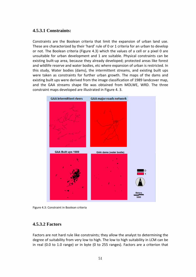
51

4.5.3.1 Constraints: Constraints are the Boolean criteria that limit the expansion of urban land use. These are characterized by their ‘hard’ rule of 0 or 1 criteria for an urban to develop or not. The Boolean criteria (Figure 4.3) which the values of a cell or a pixel 0 are unsuitable for urban development and 1 are suitable. Physical constraints can be existing built-up area, because they already developed; protected areas like forest and wildlife reserve and water bodies, etc where expansion of urban is restricted. In this study, Water bodies (dams), the intermittent streams, and existing built ups were taken as constraints for further urban growth. The maps of the dams and existing built ups were derived from the image classification of 1989 landcover map, and the GAA streams shape file was obtained from MOLWE, WRD. The three constraint maps developed are illustrated in Figure 4. 3.

Figure 4.3: Constraint in Boolean criteria

4.5.3.2 Factors

Factors are not hard rule like constraints; they allow the analyst to determining the degree of suitability from very low to high. The low to high suitability in LCM can be in real (0.0 to 1.0 range) or in byte (0 to 255 ranges). Factors are a criterion that

52

enhances or diminish from the suitability of a specific alternative for the activity under consideration (Eastman, 2006). The analyst’s criteria for low to high suitability depend on the information obtained from urban planning offices, administrators, and environmentalist or legislations bodies. It is also important to note that the analysts knowledge of the area to make important decision. For example, whether to take linear, J-shaped or sigmoid increase or decrease, during standardization of suitability ranges for the selected variables. In this study to meet the requirements of LCM and develop the criteria, the analyst has used the information collected during his field visit in Asmara. Guide line information was collected from the MLWE, Department of Environment, Department of land; and from an interview12

conducted.

4.5.3.2 Standardization of Factors Factors are not ‘hard rule’ like constraints. Constraints are Boolean in nature; they totally allow or block completely a certain area from change. In the case of factors, it is different and they give a degree of suitability for an area to change (mostly on distance basis). Hence, all the factors criteria were standardized to a continuous scale of suitability from 0 (least suitable) to 255 (most suitable) with the DISTANCE module in IDRISI. Moreover, the continuous scale has been further standardized with the FUZZY module mainly for two reasons in the case of this study. First, all the criteria could not have the same degree of suitability. Second, all areas of studies cannot have the same continuous suitability level. Therefore, based on the knowledge of the area and urbanization policy issues a Fuzzy Logic is incorporated (Table 4.1). The fuzzy module available in IDRISI, enables to standardization the whole range of the fuzzy set to membership functions type (sigmoidal, J-shape and Linear) and membership function shape (monotonically increase, decrease or symmetric). Besides, it enables us the set a control points to set the limits of the standardization. These all has been taken in consideration during the criteria development for the GAA. The following table describes the membership functions used for standardizing the variables.

_________________________________

The researcher has conducted an interview 12

(Sep.2010) with Engineer Medhanie Teklemariam, Head of Urban Planning Division, Department of Infrastructure

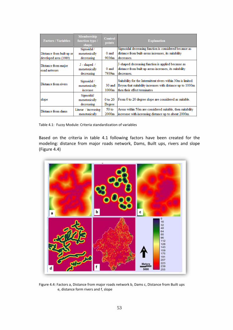
53

Table 4.1: Fuzzy Module: Criteria standardization of variables

Based on the criteria in table 4.1 following factors have been created for the modeling: distance from major roads network, Dams, Built ups, rivers and slope (Figure 4.4)

Figure 4.4: Factors a, Distance from major roads network b, Dams c, Distance from Built ups e, distance form rivers and f, slope

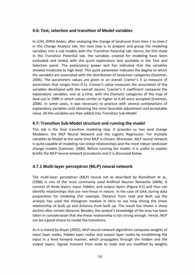
54

4.6: Test, selection and transition of Model variables In LCM, IDRISI Andes, after analyzing the change of landcover from time-1 to time-2 in the Change Analysis tab, the next step is to prepare and group the modeling variables into a sub models with the Transition Potential tab. Hence, for this study in the Transition Potential tab, the variables created for modeling have been evaluated and tested with the quick exploratory tool available in the Test and Selection panel. The explanatory power test has indicated that the variables showed moderate to high level. This quick parameter indicates the degree to which the variables are associated with the distribution of landcover categories (Eastman, 2006). The parameters values are given in an overall Cramer’s V (a measure of association that ranges from 0-1). Cramer’s value measures the association of the variables developed with the overall classes. Cramer’s V coefficient compares the explanatory variables, one at a time, with the thematic categories of the map of land use in 1989 in which values similar or higher to 0.40 were accepted (Eastman, 2006). In some cases, it was necessary to practice with several combinations of explanatory variables until obtaining the most favorable adjustment and acceptable value. All the variables are then added into Transition Sub-Model. 4.7: Transition Sub-Model structure and running the model This tab is the final transition modeling step. It provides us two land change Modelers; the MLP Neural Network and the Logistic Regression. For multiple variables to Model at the same time MLP is chosen. Moreover, MLP neural network is quite capable of modeling non-linear relationships and the most robust landcover change models (Eastman, 2006). Before running the model, it is useful to explain briefly the MLP neural network procedures and it is discussed below.

4.7.1 Multi-layer perceptron (MLP) neural network The multi-layer perceptron (MLP) neural net as described by Rumelhart et al., (1986) is one of the most commonly used Artificial Neuron Networks (ANN). It consists of three layers: input, hidden, and output layers (Figure 4.5) and thus can identify relationships that are non-linear in nature. In the case of GAA, during data preparation for modeling (For example, Distance from road and Built up) the analysis has used the Histogram module in Idrisi to see how strong the linear relationship of built up and distance from built up. The result has shown a sharp decline after certain distance. Besides, the analyst’s knowledge of the area has been taken in consideration that the linear relationship is not strong enough. Hence, MLP can be a good choice to model the transitions. As it is stated by Bryan (2002), MLP neural network algorithms computes weights of input layer nodes, hidden layer nodes and output layer nodes by establishing the input in a feed forward manner, which propagates through the hidden and the output layers. Signals transmit from node to node and are modified by weights

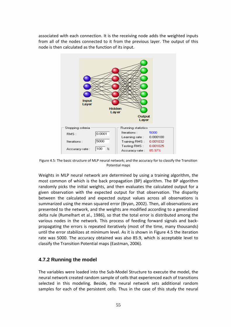
55

associated with each connection. It is the receiving node adds the weighted inputs from all of the nodes connected to it from the previous layer. The output of this node is then calculated as the function of its input.

Figure 4.5: The basic structure of MLP neural network; and the accuracy for to classify the Transition Potential maps

Weights in MLP neural network are determined by using a training algorithm, the most common of which is the back propagation (BP) algorithm. The BP algorithm randomly picks the initial weights, and then evaluates the calculated output for a given observation with the expected output for that observation. The disparity between the calculated and expected output values across all observations is summarized using the mean squared error (Bryan, 2002). Then, all observations are presented to the network, and the weights are modified according to a generalized delta rule (Rumelhart et al., 1986), so that the total error is distributed among the various nodes in the network. This process of feeding forward signals and back-propagating the errors is repeated iteratively (most of the time, many thousands) until the error stabilizes at minimum level. As it is shown in Figure 4.5 the iteration rate was 5000. The accuracy obtained was also 85.9, which is acceptable level to classify the Transition Potential maps (Eastman, 2006).

4.7.2 Running the model The variables were loaded into the Sub-Model Structure to execute the model, the neural network created random sample of cells that experienced each of transitions selected in this modeling. Beside, the neural network sets additional random samples for each of the persistent cells. Thus in the case of this study the neural

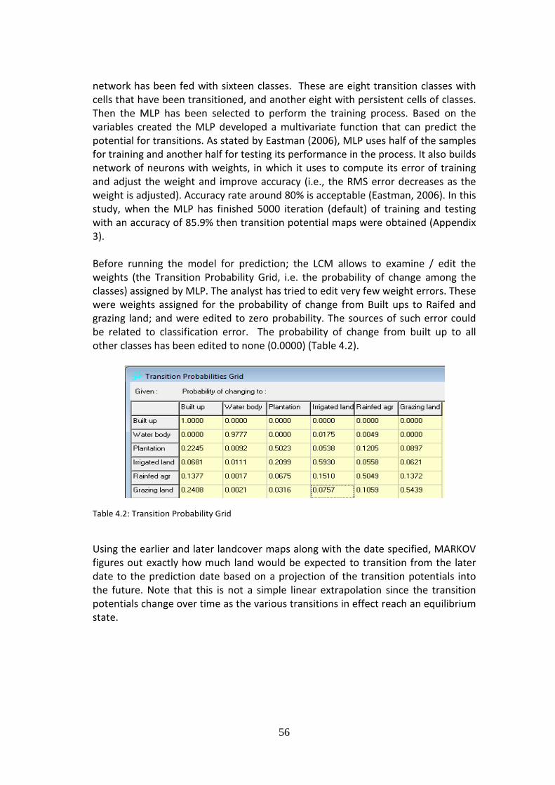
56

network has been fed with sixteen classes. These are eight transition classes with cells that have been transitioned, and another eight with persistent cells of classes. Then the MLP has been selected to perform the training process. Based on the variables created the MLP developed a multivariate function that can predict the potential for transitions. As stated by Eastman (2006), MLP uses half of the samples for training and another half for testing its performance in the process. It also builds network of neurons with weights, in which it uses to compute its error of training and adjust the weight and improve accuracy (i.e., the RMS error decreases as the weight is adjusted). Accuracy rate around 80% is acceptable (Eastman, 2006). In this study, when the MLP has finished 5000 iteration (default) of training and testing with an accuracy of 85.9% then transition potential maps were obtained (Appendix 3). Before running the model for prediction; the LCM allows to examine / edit the weights (the Transition Probability Grid, i.e. the probability of change among the classes) assigned by MLP. The analyst has tried to edit very few weight errors. These were weights assigned for the probability of change from Built ups to Raifed and grazing land; and were edited to zero probability. The sources of such error could be related to classification error. The probability of change from built up to all other classes has been edited to none (0.0000) (Table 4.2).

Table 4.2: Transition Probability Grid Using the earlier and later landcover maps along with the date specified, MARKOV figures out exactly how much land would be expected to transition from the later date to the prediction date based on a projection of the transition potentials into the future. Note that this is not a simple linear extrapolation since the transition potentials change over time as the various transitions in effect reach an equilibrium state.

57

4.8: Change prediction and validation

4.8.1 Change prediction Change Prediction tab, is a third tab next to change analysis and Transition potential tab in LCM steps in IDRISI. This tab provides the controls for a dynamic land cover change prediction process by specifying an end year. The default modeler is Markov Chain analysis, which allows the transition likelihood of one pixel to be a function of nearest pixels, a pixel is highly influenced by its nearby pixel (Pontius and Chen, 2006). Markov Chain Analysis is a convenient tool for modeling landuse change when changes and processes in the landscape are difficult to describe (Eastman, 2006). A Markovian process is simply one in which the future state of a system can be modeled purely on the basis of the immediately preceding state. Markov Chain Analysis describes landuse change from one period to another to project future changes. This is accomplished by developing a transition probability matrix (Table 4.2) of landuse change from time-1 (GAA in 1989) to time-2 (GAA in 2000), which has the basis for projecting to a later time period (GAA in 2009). In the Change Prediction tab, two modelers of change are provided: the hard prediction which gives only a single realization; and the soft prediction which gives a comprehensive assessment of change potential. A change prediction date for 2009 has first been selected and created with soft prediction. A soft prediction was chosen for its advantage of mapping of areas that are possible candidate for change. It provides a continuous map of vulnerability to change for the selected set of transitions. Besides, based on the tests the analyst has done it produced more accurate map. The 2009 has been simulated in order to compare with the ‘actual’ LUCC 2009 of GAA. When compared visually the predicted 2009 with the ‘actual’ or classified LUCC 2009 (Figure 4.6), the maps showed noticeably differences. This was as expected and true that the history of change from 1989 to 2000 cannot be the same with the history of change from 2000 to 2009. Besides, the variables have been created with more focus on the Built up areas, and this has played a role on the other classes to stay more unchanged (Eastman, 2006). More importantly, in the case of Eritrea where the government owns all land, Land Reform Proclamation (No. 58/1994), the changes in land allocation policy, land use policy and the interruption of construction are not easy to predict. Eastman (2006) has also stated that past history is not always a good indicator of the future. Nonetheless, as it is stated by Cabral et. al., (2009) though insufficient for spatial explicit LUCC predictions, Markov Chain constitute a good tool for describing and projecting LUCC quantities.

4.8.2 Validation The simulation for the map of 2009 has been performed with the Markov module. As stated by Cabral et al., (2006) the Markov module is based on the first law of Geography that is the rule of contiguity. The rule which states a probability of a cell

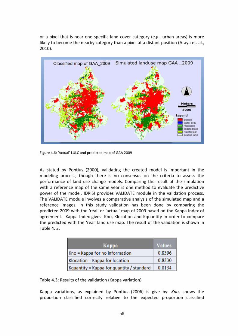
58

or a pixel that is near one specific land cover category (e.g., urban areas) is more likely to become the nearby category than a pixel at a distant position (Araya et. al., 2010).

Figure 4.6: ‘Actual’ LULC and predicted map of GAA 2009 As stated by Pontius (2000), validating the created model is important in the modeling process, though there is no consensus on the criteria to assess the performance of land use change models. Comparing the result of the simulation with a reference map of the same year is one method to evaluate the predictive power of the model. IDRISI provides VALIDATE module in the validation process. The VALIDATE module involves a comparative analysis of the simulated map and a reference images. In this study validation has been done by comparing the predicted 2009 with the ‘real’ or ‘actual’ map of 2009 based on the Kappa Index of agreement. Kappa Index gives: Kno, Klocation and Kquantity in order to compare the predicted with the ‘real’ land use map. The result of the validation is shown in Table 4. 3.

Table 4.3: Results of the validation (Kappa variation) Kappa variations, as explained by Pontius (2006) is give by: Kno, shows the proportion classified correctly relative to the expected proportion classified

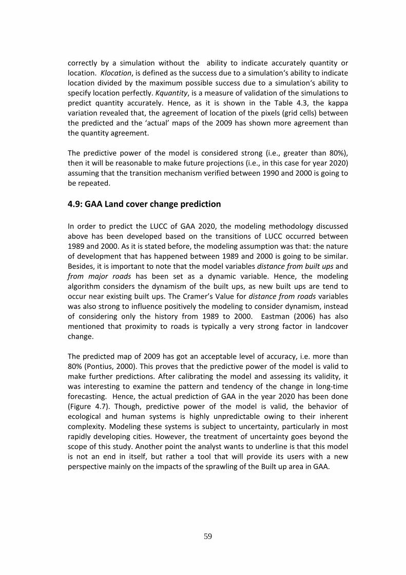
59

correctly by a simulation without the ability to indicate accurately quantity or location. Klocation, is defined as the success due to a simulation‘s ability to indicate location divided by the maximum possible success due to a simulation‘s ability to specify location perfectly. Kquantity, is a measure of validation of the simulations to predict quantity accurately. Hence, as it is shown in the Table 4.3, the kappa variation revealed that, the agreement of location of the pixels (grid cells) between the predicted and the ‘actual’ maps of the 2009 has shown more agreement than the quantity agreement. The predictive power of the model is considered strong (i.e., greater than 80%), then it will be reasonable to make future projections (i.e., in this case for year 2020) assuming that the transition mechanism verified between 1990 and 2000 is going to be repeated. 4.9: GAA Land cover change prediction In order to predict the LUCC of GAA 2020, the modeling methodology discussed above has been developed based on the transitions of LUCC occurred between 1989 and 2000. As it is stated before, the modeling assumption was that: the nature of development that has happened between 1989 and 2000 is going to be similar. Besides, it is important to note that the model variables distance from built ups and from major roads has been set as a dynamic variable. Hence, the modeling algorithm considers the dynamism of the built ups, as new built ups are tend to occur near existing built ups. The Cramer’s Value for distance from roads variables was also strong to influence positively the modeling to consider dynamism, instead of considering only the history from 1989 to 2000. Eastman (2006) has also mentioned that proximity to roads is typically a very strong factor in landcover change. The predicted map of 2009 has got an acceptable level of accuracy, i.e. more than 80% (Pontius, 2000). This proves that the predictive power of the model is valid to make further predictions. After calibrating the model and assessing its validity, it was interesting to examine the pattern and tendency of the change in long-time forecasting. Hence, the actual prediction of GAA in the year 2020 has been done (Figure 4.7). Though, predictive power of the model is valid, the behavior of ecological and human systems is highly unpredictable owing to their inherent complexity. Modeling these systems is subject to uncertainty, particularly in most rapidly developing cities. However, the treatment of uncertainty goes beyond the scope of this study. Another point the analyst wants to underline is that this model is not an end in itself, but rather a tool that will provide its users with a new perspective mainly on the impacts of the sprawling of the Built up area in GAA.

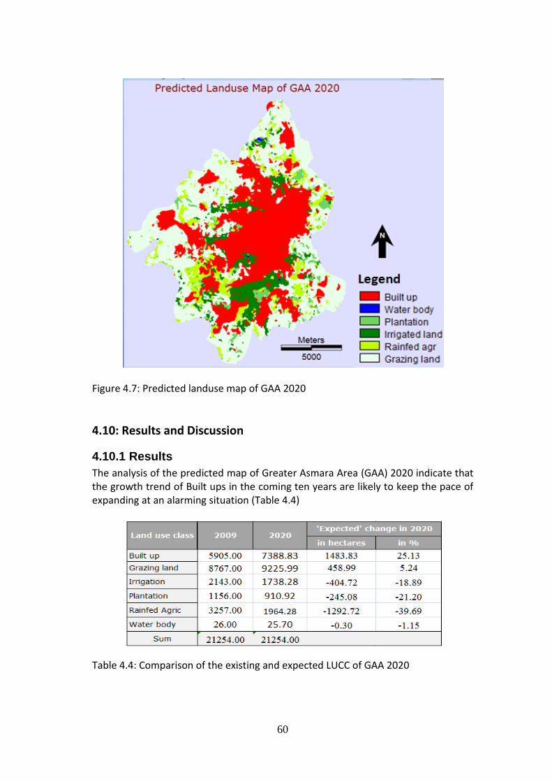
60

Figure 4.7: Predicted landuse map of GAA 2020 4.10: Results and Discussion

4.10.1 Results The analysis of the predicted map of Greater Asmara Area (GAA) 2020 indicate that the growth trend of Built ups in the coming ten years are likely to keep the pace of expanding at an alarming situation (Table 4.4)

Table 4.4: Comparison of the existing and expected LUCC of GAA 2020

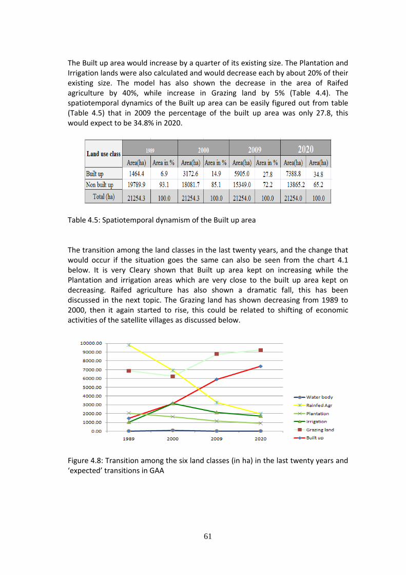
61

The Built up area would increase by a quarter of its existing size. The Plantation and Irrigation lands were also calculated and would decrease each by about 20% of their existing size. The model has also shown the decrease in the area of Raifed agriculture by 40%, while increase in Grazing land by 5% (Table 4.4). The spatiotemporal dynamics of the Built up area can be easily figured out from table (Table 4.5) that in 2009 the percentage of the built up area was only 27.8, this would expect to be 34.8% in 2020.

Table 4.5: Spatiotemporal dynamism of the Built up area The transition among the land classes in the last twenty years, and the change that would occur if the situation goes the same can also be seen from the chart 4.1 below. It is very Cleary shown that Built up area kept on increasing while the Plantation and irrigation areas which are very close to the built up area kept on decreasing. Raifed agriculture has also shown a dramatic fall, this has been discussed in the next topic. The Grazing land has shown decreasing from 1989 to 2000, then it again started to rise, this could be related to shifting of economic activities of the satellite villages as discussed below.

Figure 4.8: Transition among the six land classes (in ha) in the last twenty years and ‘expected’ transitions in GAA

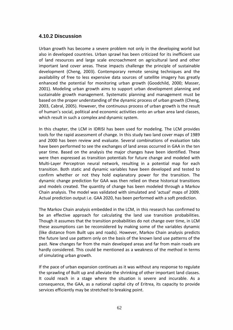
62

4.10.2 Discussion Urban growth has become a severe problem not only in the developing world but also in developed countries. Urban sprawl has been criticized for its inefficient use of land resources and large scale encroachment on agricultural land and other important land cover areas. These impacts challenge the principle of sustainable development (Cheng, 2003). Contemporary remote sensing techniques and the availability of free to less expensive data sources of satellite imagery has greatly enhanced the potential for monitoring urban growth (Goodchild, 2000; Masser, 2001). Modeling urban growth aims to support urban development planning and sustainable growth management. Systematic planning and management must be based on the proper understanding of the dynamic process of urban growth (Cheng, 2003, Cabral, 2005). However, the continuous process of urban growth is the result of human’s social, political and economic activities onto an urban area land classes, which result in such a complex and dynamic system. In this chapter, the LCM in IDRISI has been used for modeling. The LCM provides tools for the rapid assessment of change. In this study two land cover maps of 1989 and 2000 has been review and evaluate. Several combinations of evaluation tabs have been performed to see the exchanges of land areas occurred in GAA in the ten year time. Based on the analysis the major changes have been identified. These were then expressed as transition potentials for future change and modeled with Multi-Layer Perceptron neural network, resulting in a potential map for each transition. Both static and dynamic variables have been developed and tested to confirm whether or not they hold explanatory power for the transition. The dynamic change prediction for GAA was then relied on these historical transitions and models created. The quantity of change has been modeled through a Markov Chain analysis. The model was validated with simulated and ‘actual’ maps of 2009. Actual prediction output i.e. GAA 2020, has been performed with a soft prediction. The Markov Chain analysis embedded in the LCM, in this research has confirmed to be an effective approach for calculating the land use transition probabilities. Though it assumes that the transition probabilities do not change over time, in LCM these assumptions can be reconsidered by making some of the variables dynamic (like distance from Built ups and roads). However, Markov Chain analysis predicts the future land use pattern only on the basis of the known land use patterns of the past. New changes far from the main developed areas and far from main roads are hardly considered. This could be mentioned as a weakness of the method in terms of simulating urban growth. If the pace of urban expansion continues as it was without any response to regulate the sprawling of Built up and alleviate the shrinking of other important land classes. It could reach in a stage where the situation is severe and incurable. As a consequence, the GAA, as a national capital city of Eritrea, its capacity to provide services efficiently may be stretched to breaking point.

63

The dramatic fall in Raifed agriculture (Chart 4.1) that has observed and would expected to continue can be analyzed in association with the shift of economic activities (i.e. to non farming activities) of many ‘satellite villages’. Thought, the satellite villages would be urbanized, it is also another alarming situation that the agricultural areas would be abandoned. This may lead to a serious consequence of food shortage. The shrinking size of land for irrigation and the abandonment of Raifed agriculture would impact negatively to the total food production and might aggravate food insecurity in the area. Approximately, 80% of the people of Eritrea earn their living from economic activities related to agriculture (crop and livestock production) (Wolfe et al., 2008). However, urban agriculture hasn’t got much attention to adopt a policy of regulating and promoting it (NAP, 2002). Besides, during the National Action programme (NAP, 2002) for Eritrea to combat desertification and mitigate the effects of drought, it has been discussed that the sprawling of GAA would cause urban hunger due to loss of urban agriculture; change in soil characteristics which would lead to soil degradation; and loss of land for subsistence agriculture (loss of livelihood) et cetera.

64

CHAPTER FIVE

Conclusions and recommendations 5.1: Conclusions Urban growth and the concentration of people in urban areas are growing steadily specially in the developing countries. Most growth are uncoordinated, which result in serious environmental and social problems (Leao, 2004). The GAA the main focus of this study, which is Asmara and the nearby thirteen satellite villages, is scene of intense competition between urban expansion and agricultural land uses, concern of environmental degradation, challenges in urban planning and proper land resource allocation. In the last two decades, GAA have experienced a rapid growth which resulted in loss of valuable land of urban agriculture, decline in natural vegetation cover and uncoordinated outward sprawling. Based on these alarming issues, a research interest was initiated, in order to provide basic information on the status and dynamics of the rate of urban growth and urban landuse changes of the study area. Thus, the finding might be used to support in decision making to mitigate the problem. The overall research objective was to detect land use change, quantify and analyze the change and finally to develop a model and predict the future land use change. Progress in modern remote sensing and GIS techniques has opened up great opportunities, and significant success has already been achieved in monitoring and managing fast urban growth. Hence, to meet these objectives, it was essential to integrate and apply geospatial technologies like

remote sensing, GIS and spatial modeling tool.

Overall the research comprises five chapters, whereas Chapter 2, 3 and 4 are the core chapters. Chapter 1 provides a general overview of the research. Relevant literatures related to causes and consequences of urban growth, the importance of the study, objectives and scope, the data used and the way the analyst approached the research techniques and methods are discussed. Chapter 2 focuses mainly on producing maps of the study area from satellite images. Data pre-processing and image classification with the applications of remote sensing techniques have been performed. Object oriented image classification has been employed. Validation of classification results is an important process after image classification procedure. Hence, the classified images were then validated. The validation was done both in eCognition, sample based validation. Moreover, validation was done based on the reference map. In both cases, Kappa coefficient has found to be above the minimum threshold. This chapter has taken considerable time and care, as the three maps for the three time periods (1989, 2000 and 2009) would be the inputs of the whole thesis process. More focus has also been given for Built up areas as they are the main focus of the study.

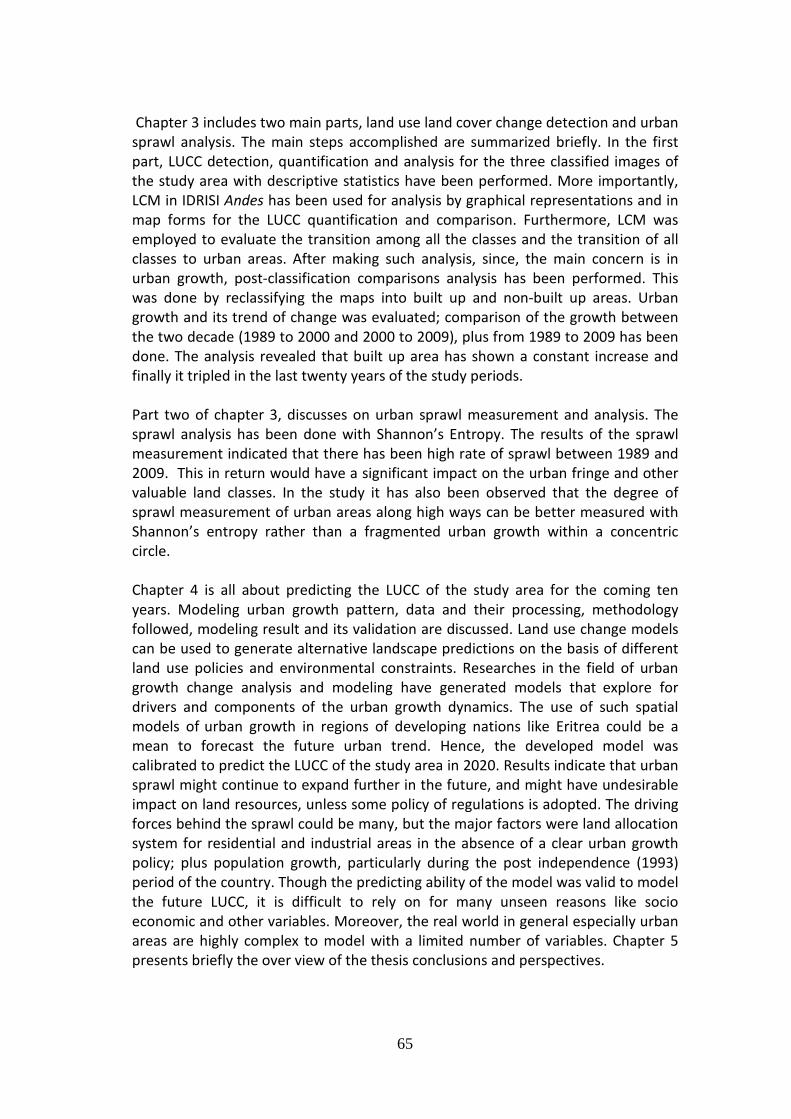
65

Chapter 3 includes two main parts, land use land cover change detection and urban sprawl analysis. The main steps accomplished are summarized briefly. In the first part, LUCC detection, quantification and analysis for the three classified images of the study area with descriptive statistics have been performed. More importantly, LCM in IDRISI Andes has been used for analysis by graphical representations and in map forms for the LUCC quantification and comparison. Furthermore, LCM was employed to evaluate the transition among all the classes and the transition of all classes to urban areas. After making such analysis, since, the main concern is in urban growth, post-classification comparisons analysis has been performed. This was done by reclassifying the maps into built up and non-built up areas. Urban growth and its trend of change was evaluated; comparison of the growth between the two decade (1989 to 2000 and 2000 to 2009), plus from 1989 to 2009 has been done. The analysis revealed that built up area has shown a constant increase and finally it tripled in the last twenty years of the study periods. Part two of chapter 3, discusses on urban sprawl measurement and analysis. The sprawl analysis has been done with Shannon’s Entropy. The results of the sprawl measurement indicated that there has been high rate of sprawl between 1989 and 2009. This in return would have a significant impact on the urban fringe and other valuable land classes. In the study it has also been observed that the degree of sprawl measurement of urban areas along high ways can be better measured with Shannon’s entropy rather than a fragmented urban growth within a concentric circle. Chapter 4 is all about predicting the LUCC of the study area for the coming ten years. Modeling urban growth pattern, data and their processing, methodology followed, modeling result and its validation are discussed. Land use change models can be used to generate alternative landscape predictions on the basis of different land use policies and environmental constraints. Researches in the field of urban growth change analysis and modeling have generated models that explore for drivers and components of the urban growth dynamics. The use of such spatial models of urban growth in regions of developing nations like Eritrea could be a

mean to forecast the future urban trend. Hence, the developed model was calibrated to predict the LUCC of the study area in 2020. Results indicate that urban sprawl might continue to expand further in the future, and might have undesirable impact on land resources, unless some policy of regulations is adopted. The driving forces behind the sprawl could be many, but the major factors were land allocation system for residential and industrial areas in the absence of a clear urban growth policy; plus population growth, particularly during the post independence (1993) period of the country. Though the predicting ability of the model was valid to model the future LUCC, it is difficult to rely on for many unseen reasons like socio economic and other variables. Moreover, the real world in general especially urban areas are highly complex to model with a limited number of variables. Chapter 5 presents briefly the over view of the thesis conclusions and perspectives.

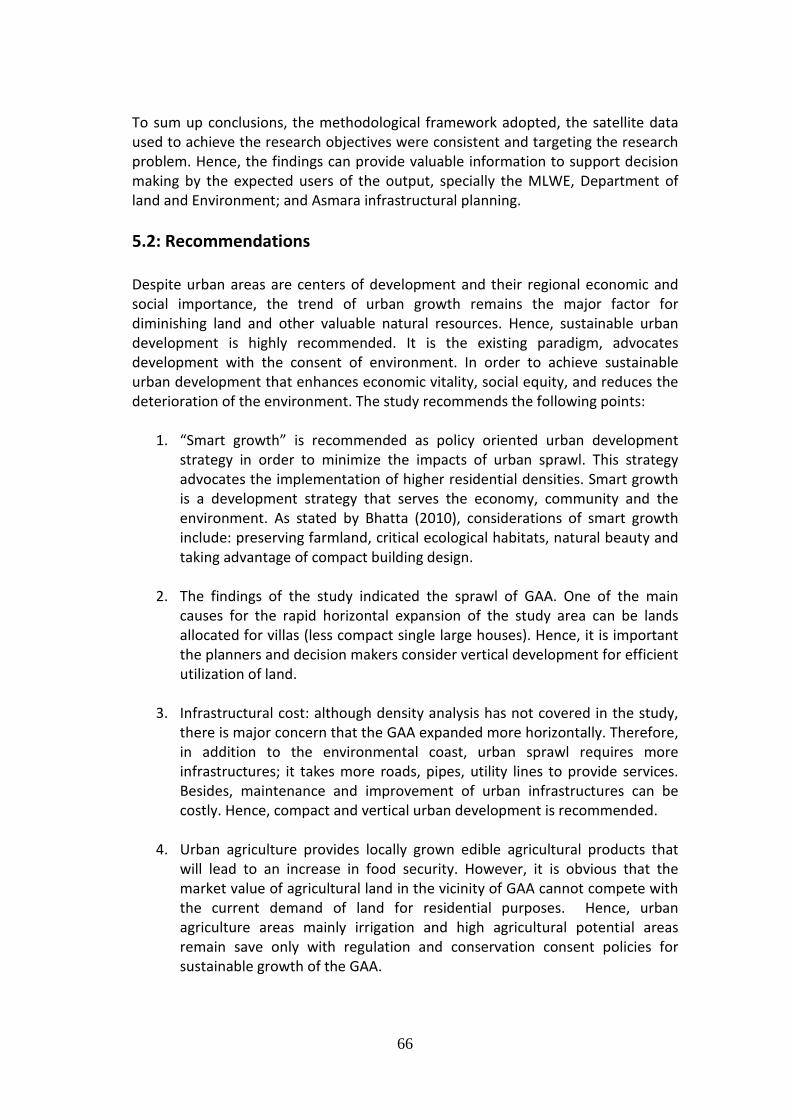
66

To sum up conclusions, the methodological framework adopted, the satellite data used to achieve the research objectives were consistent and targeting the research problem. Hence, the findings can provide valuable information to support decision making by the expected users of the output, specially the MLWE, Department of land and Environment; and Asmara infrastructural planning. 5.2: Recommendations Despite urban areas are centers of development and their regional economic and social importance, the trend of urban growth remains the major factor for diminishing land and other valuable natural resources. Hence, sustainable urban development is highly recommended. It is the existing paradigm, advocates development with the consent of environment. In order to achieve sustainable urban development that enhances economic vitality, social equity, and reduces the deterioration of the environment. The study recommends the following points:

1. “Smart growth” is recommended as policy oriented urban development strategy in order to minimize the impacts of urban sprawl. This strategy advocates the implementation of higher residential densities. Smart growth is a development strategy that serves the economy, community and the environment. As stated by Bhatta (2010), considerations of smart growth include: preserving farmland, critical ecological habitats, natural beauty and taking advantage of compact building design.

2. The findings of the study indicated the sprawl of GAA. One of the main causes for the rapid horizontal expansion of the study area can be lands allocated for villas (less compact single large houses). Hence, it is important the planners and decision makers consider vertical development for efficient utilization of land.

3. Infrastructural cost: although density analysis has not covered in the study, there is major concern that the GAA expanded more horizontally. Therefore, in addition to the environmental coast, urban sprawl requires more infrastructures; it takes more roads, pipes, utility lines to provide services. Besides, maintenance and improvement of urban infrastructures can be costly. Hence, compact and vertical urban development is recommended.

4. Urban agriculture provides locally grown edible agricultural products that will lead to an increase in food security. However, it is obvious that the market value of agricultural land in the vicinity of GAA cannot compete with the current demand of land for residential purposes. Hence, urban agriculture areas mainly irrigation and high agricultural potential areas remain save only with regulation and conservation consent policies for sustainable growth of the GAA.

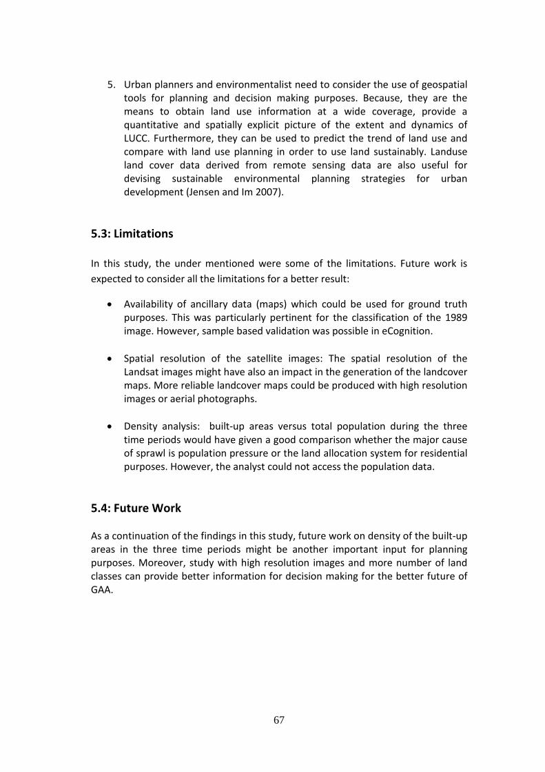
67

5. Urban planners and environmentalist need to consider the use of geospatial tools for planning and decision making purposes. Because, they are the means to obtain land use information at a wide coverage, provide a quantitative and spatially explicit picture of the extent and dynamics of LUCC. Furthermore, they can be used to predict the trend of land use and compare with land use planning in order to use land sustainably. Landuse land cover data derived from remote sensing data are also useful for devising sustainable environmental planning strategies for urban development (Jensen and Im 2007).

5.3: Limitations In this study, the under mentioned were some of the limitations. Future work is expected to consider all the limitations for a better result:

• Availability of ancillary data (maps) which could be used for ground truth purposes. This was particularly pertinent for the classification of the 1989 image. However, sample based validation was possible in eCognition.

• Spatial resolution of the satellite images: The spatial resolution of the Landsat images might have also an impact in the generation of the landcover maps. More reliable landcover maps could be produced with high resolution images or aerial photographs.

• Density analysis: built-up areas versus total population during the three time periods would have given a good comparison whether the major cause of sprawl is population pressure or the land allocation system for residential purposes. However, the analyst could not access the population data.

5.4: Future Work As a continuation of the findings in this study, future work on density of the built-up areas in the three time periods might be another important input for planning purposes. Moreover, study with high resolution images and more number of land classes can provide better information for decision making for the better future of GAA.

68

Bibliography

Alkheder, S. and Shan, S. (2005). Cellular Automata Urban Growth Simulation and Evaluation-a case study of Indianapolis. http://geocomputation.org/2005/Alkheder.pdf Accessed 12 April 2010 Abraham Daniel; Filmon Tefasslasie; Selamawit Tesfay (2009). An Appraisal of the Current Status and the Potential of Surface Water in Upper Anseba Catchment, Eritrea; SLM Eritrea. Abuelgasim, A., W. Ross, et al. (1999). Change Detection using Adaptive Fuzzy neural networks: Environmental damage assessment after the Gulf War. Remote Sensing of Environment 70(2): 208-223. Africover: Specifications for geometry and cartography, summary report of the workshop on Africover, 2000 (E) Agarwal, C., Green, G. L., Grove, J. M., Evans, T., and Schweik, C. (2000). “A review and assessment of land use change models: dynamics of space, time, and human choice.” 4th International Conference on Integrating GIS and Environmental Modeling (GIS/EM4): Problems, Prospects and Research Needs, Banff, Alberta, Canada.

Anderson, J. R., E. E. Hardy, et al. (1976). A Land Use And Land Cover Classification System For Use With Remote Sensor Data, U.S. Geological Survey. [online] http://landcover.usgs.gov/pdf/anderson.pdf [accessed on Nov.20, 2010] Andreas Heinimann, Thomas Breu, and Thomas Kohler (2003). The Challenge of Applying Geographic Information Systems to Sustainable Mountain Development. International Mountain Society [online] http://www.bioone.org/doi/pdf/10.1659/0276-4741%282003%29023%5B0312%3ATCOAGI%5D2.0.CO%3B2 [accessed on Dec. 2010] Angel, Schlomo, Stephen C. Sheppard, and Daniel L. Civco, et al. (2005). The Dynamics of Global Urban Expansion. Transport and Urban Development, The World Bank. Araya, Y. H. and C. Hergarten. (2008). A Comparison of Pixel and Object-based Land cover Classification: A Case Study of Asmara, Eritrea. In proceedings of Geo-Environment and Landscape Evolution III Vol. 100. pp. 233-243 Araya Y.H., Cabral P. (2010). Analysis and Modeling of Urban Land Cover Change in Setúbal and Sesimbra, Portugal. Remote Sensing. Vol. 2, 1549-1563. [online] http://www.mdpi.com/2072-4292/2/6/1549/pdf [accessed on Oct. 2010] BCEOM/Groupe Huit-Optima (2006), Asmara Infrastructure Development Study, Executive Summary of the Strategic Urban Development Plan, BCEOM/Groupe Huit-Optima, July 2006, p11 BCEOM/Groupe Huit-Optima (2006), Asmara Infrastructure Development Study, Executive Summary of the Strategic Urban Development Plan, BCEOM/Groupe Huit-Optima, July 2006, p8 Belaid, M. (2003). Urban-Rural Land use Change Detection Analysis Using GIS and Remote Sensing Technologies.2nd FIG Regional conference, Marrakech, Morocco. Benz, U. C., P. Hofmann, G. Willhauck, I. Lingenfelder & M. Heynen, 2004. Multi-resolution, object-oriented fuzzy analysis of remote sensing data for GIS-ready information. Isprs Journal of Photogrammetry and Remote Sensing, 58, 239-258.

Berkavoa, V. (2007). Application of Remote Sensing and GIS for Change Detection from Various

69

Data Type of Remote Sensing.

Bhatta, B. (2010). Analysis of urban growth and sprawl from remote sensing data. Berlin, Heidelberg: Springer-Verlag. [online] http://www.springerlink.com/content/978-3-642-05298-9#section=663397&page=1&locus=69 [Dec 2010] Bhatta, B., Saraswati, S. and Bandyopadhyay, D. (2010a). Quantifying the degree-of-freedom, degree-of-sprawl, and degree-of-goodness of urban growth from remote sensing data. Applied Geography, 30(1), 96–111. Buiton, P.J. (1994). A vision for equitable land use allocation. Land Use Policy, 12(1), 63–68.Buliung, R.N. and Kanaroglou, P.S. (2006). Urban form and household activity travel behavior. Growth and Change, 37, 172–178. Burchell RW, Shad N A, Listokin D, Phillips H, Seskin S, Davis J S, Moore T, Helton D, Gall M, 1998. The Costs of SprawlöRevisited: Transportation Research Board Report 39 (National Academy Press,Washington, DC) CABRAL, P.; GILG J.-P.; PAINHO M. (2005). Monitoring urban growth using remote sensing, GIS and spatial metrics. Proceedings of SPIE Optics & Photonics: Remote sensing and modeling of ecosystems for sustainability. San Diego, USA. pp. 1-9. Cabral, P. (2006). ÉTUDE DE LA CROISSANCE URBAINE PAR TÉLÉDÉTECTION, SIG ETMODÉLISATION Le cas des Concelhos de Sintra et Cascais (Portugal) Cabral, P., Geroyannis, H., Gilg, J., Painho,M. (2006). Analysis and modeling of land-use and land-cover change in Sintra-Cascais area. [online] http://plone.itc.nl/agile_old/Conference/estoril/papers/06_Pedro%20Cabral.pdf [Accessed Dec 2010] Cabral, P.; Zamyatin, A. (2006) Three land change models for urban dynamics analysis in Sintra-Cascais area. In Proceedings of the 1st EARSel Workshop of the SIG Urban remote sensing, Humboldt-Universität zu Berlin, Berlin, Germany. Cabral, Pedro and Zamyatin, Alexander. (2009). Markov processes in modeling land use and land cover changes in sintra-cascais, portugal. Dyna rev.fac.nac.minas, vol.76, no.158, p.191-198. ISSN 0012-7353. [on line] http://www.scielo.unal.edu.co/scielo.php?pid=S0012-73532009000200018&script=sci_arttext [accessed on Dec. 2010] Charles D Wende of NASA Headquarters. Landsat tutorials.

. [on line] https://zulu.ssc.nasa.gov/mrsid/tutorial/Landsat%20Tutorial-V1.html [accessed on Dec 2010]

CHENG, J. (2003). Modeling Spatial & Temporal Urban Growth. PhD thesis Utrecht University. Faculty of Geographical Sciences Clark labs (2009). Land Change Modeler feature Overview. [on line] http://www.clarklabs.org/products/upload/LCM_Feature_Overview.pdf [accessed on December 2010] Congalton, R.G. (1991). A review of assessing the accuracy of classifications of remotely sensed data. Remote Sens. Environ. 37, 35-46. D. LU, P. MAUSEL, E. BRONDI ´ZIO and E. MORAN (2004). Change detection techniques. INT. J. REMOTE SENSING. [online]

70

http://www.indiana.edu/~act/files/Dengsheng/change_detection_techniques_IJRS_2004.pdf [accessed on Oct 2010]

Definiens, 2009. eCognition Developer 8 Reference Book, Version 1.2.0, User Guide, Definiens AG, München, Germany, 34-38 p. Eastman, R. J. (2006). IDRISI Andes, Guide to GIS and Image Processing. Clark University, Worcester. pp 87-131. Eastman. J. Ronald, (2006). IDRISI Andes Tutorial. Clark Labs Clark University, Worcester, MA, 00USA Manual Version 15. [on line] http://www.geog.ubc.ca/courses/geob373/labs/Andes_Tutorial.pdf [accessed Nov. 2010] eCognition, (2010). eCognition 8.0: Guided Tour Level 1, Version 3.0, Getting started – Example: Simple building extraction Classification of buildings using elevation and RGB data. Erdas Imagine9.2 User manual. [online]. http://gi.leicageosystems.com/documents/pdf/Training_Manual_Order_Form.pdf [accessed on Nov. 17, 2010] FAO (2006), Country profile. [on line] http://www.fao.org/ag/AGP/AGPC/doc/Counprof/eritrea/Eritrea.htm [accessed on Oct. 2010] FULLER, R. M., SMITH, G. M., SANDERSON, J. M., HILL, R. A., and HOMSON, A. G., 2002, Land Cover Map 2000: construction of a parcel-based vector map from satellite images. Cartographic Journal, 39, 15–25. Fuller, R.M., Smith, G.M., and Devereux, B.J. (2003). The characterization and measurement of land cover change through remote sensing: problems in operational applications? International Journal of Applied Earth Observation, 4, 243–253. Gluch, R. (2002). Urban growth detection using texture analysis on merged Landsat TM and SPOT-P data. Photogrammetric Engineering & Remote Sensing 68(12): 1283-1288 Goodchild, M. F. (2000). “Spatial analysis: methods and problems in land use management.” in Spatial Information for Land Use Management, eds. M. J. Hill and R. J. Aspinall, (Gordon and Breach Science Publishers, Singapore), 39-50. Herold, M., Scepan, J. and Clarke, C. (2002). The use of remote sensing and landscape metrics to describe structures and changes in urban land uses. ENVIRONMENT AND PLANNING A 34(8): 1443-1458 Herold, M.; Goldstein, N.C.; Clarke, K.C (2003). The spatiotemporal form of urban growth: measurement, analysis and modelling. Remote Sens. Environ. 86, 286-302 Housing/Urban Development Policy Report (2005) [on line] https://habnet.unhabitat.org/files/6670_FINAL_Consolidated_Policy_Report_Eritrea_July20.pdf [accessed on Oct. 2010] IDRISI Focus Paper (2009). The Land Change Modeler for Ecological Sustainability. Clark Labs. [on line] http://www.clarklabs.org/applications/upload/Land-Change-Modeler-IDRISI-Focus-Paper.pdf [accessed on Oct. 2010]

71

Im, J., Jensen, J. and Tullis J. (2008). "Object-based change detection using correlation image analysis and image segmentation." International Journal of Remote Sensing 29(2): 399-423. Im, J., Jensen, J.R., 2005. A change detection model based on neighborhood correlation image analysis and decision tree classification. Remote Sensing of Environment 99,pp. 326 – 340

Intergovernmental Panel on Climate Change. 2007. Climate Change 2007: The Physical Science Basis: Summary for Policy Makers. Geneva: Intergovernmental Panel on Climate Change. [online] http://www.ipcc.ch/pdf/supporting-material/tgica_reg-meet-fiji-2007.pdf, [accessed 29 May. 2010] Jensen, J.R., Cowen, D.J., Althausen, J.D., Nanunalani, S. and Weatherbee, O. (1993). An evaluation of the CoastWatch change detection protocol in South Carolina. Photogrammetric Engineering and Remote Sensing, 59(6), 1039–1046. Jensen, J. R. (1996). Introductory Digital Image Processing: A Remote Sensing Perspective. 2ded.Englewood Cliffs, New Jersey: Prentice-Hall. Jensen, R., Gatrell, J., and Mclean, D. (2005). Geo-spatial technologies in urban environments, Springer. Jensen, J.R. (2006). Remote Sensing of the Environment: An Earth Resource Perspective, 2nd ed., Prentice Hall, Upper Saddle River, NJ, p. 592. Jensen, J.R. and Im, J. (2007). Remote sensing change detection in urban environments. In: R.R. Jensen, J.D. Gatrell and D. McLean (eds.), Geo-Spatial Technologies in Urban Environments: Policy, Practice and Pixels, 2nd ed., Springer-Verlag, Heidelberg, pp. 7–30. Kaiser M. et. al. (2008). Spectral Enhancement of the SPOT Imagery Data to Assess Marine Pollution near Port Said, Egypt. In PIERS Proceedings, Cambridge, USA, July 2-6. pp 746-753 Kaufmann, R. and K. Seto (2001). Change detection, accuracy, and bias in a sequential analysis of Landsat imagery in the Pearl River Delta, China: econometric techniques. Agriculture, Ecosystems and Environment 86: 286-302. Lee, J., et al., (1999). Development of a community-accessible urban sprawl impact assessment system in Northeast Ohio, 15-county region for the impact project. Washington, DC, US [on line] http://gis.kent.edu/gis/empact/filelib/review.pdf [accessed on November 2010] Leta, M., Prasad, K., Bandarinath, K., Raghavaswamy, R. and Rao, S. (2001). Measuring urban sprawl: A case study of Hyderabad. Map India. Lewinski, S. (2006). Applying fused multispectral and panchromatic data of Landsat ETM+ to object oriented classification. Proccedings of the 26th EARSeL Symposium, New Developments and Challenges in Remote Sensing, May 29-June 2, 2006, Warsaw, Poland. Li, X.; Yeh, A.G.-O. (2004). Analyzing spatial restructuring of land use patterns in a fast growing region using remote sensing and GIS. Landscape Urban Plan. 69, 335-354 Lilesand.T and Kiefer.R. (2002): Remote Sensing and Image Interpretation , John Wiley & Sons, Inc.NewYork Lu, D. and Weng, Q. (2004). Spectral mixture analysis of the urban landscape in Indianapolis with Landsat ETM+ imagery. Photogrammetric Engineering and Remote Sensing, 70(9), 1053–1062

72

Masek, J., F. Lindsay, et al. (2000). Dynamics of urban growth in the Washington DC metropolitan area, 1973-1996, from Landsat observations. International Journal of Remote Sensing 21(18): 3473-3486. Masser, I. (2001). “Managing our urban future: the role of remote sensing and geographic information systems.” Habitat International, 25, 503-512.

Matinfar, H.R. (2007). Comparisons of Object-Oriented and Pixel-Based Classification of Land Use/Land Cover Types Based on Landsat7, Etm+ Spectral Bands (Case Study: Arid Region of Iran) [Electronic version]. American-Eurasian J. Agric. & Environ. Sci., 2 (4): 448-456. Michael P Johnson, 2001. Environmental impacts of urban sprawl: a survey of the literature and proposed research agenda. Environment and Planning, volume 33, pages 717 ^ 735 Carnegie. [online] http://www-agecon.ag.ohiostate.edu/class/AEDE680/Irwin/pdf/93.pdf [accessed on Nov 2010] MoA, 2002. The National Action Program for Eritrea to Combat Desertification and Mitigate the Efforts of Drought (NAP). MoA, Eritrea. MOLWE-DoE, 2006. Support the development of legislative and regulatory framework and the strengthening of government’s capacity for effective Natural Resources Management, Asmara, MOLWE-DoE. MUCHER, C.; STEINNOCHER K.; KRESSLER F. (2000). Land cover characterization and change detection for environmental planning of Pan-Europe. International Journal of Remote Sensing, Vol. 21. pp. 1159-1181. Navulur, K., 2007. Multispectral image analysis using the object-oriented paradigm, CRC Press, Boca Raton, FL. 165 pp. [online] http://www.wy.blm.gov/prbgroup/08july/QB-AqHabMapping.pdf [accessed on 25 Nov, 2010] Negassi, A., Bein, E., Ghebru, K. and Tengnas, B. 2002. Soil and Water Conservation Manual for Eritrea. RELMA Technical Handbook Series 29. Nairobi, Kenya. [online] http://www.worldagroforestry.org/units/Library/books/Book%20100/soil%20and%20water%20conservation%20manual%20for%20eritrea/erithrea/html/index.htm [accessed on Dec 2010] Pendall R, 1999, ``Do land-use controls cause sprawl?'' Environment and Planning B: Planning and Design 26 555 ^ 571 [online] http://ideas.repec.org/a/pio/envirb/v26y1999i4p555-571.html [accessed on November 2010] Pijanowski, B.C., D. G. Brown, G. Manik and B. Shellito. 2002. Using Neural Nets and GIS to Forecast Land Use Changes: A Land Transformation Model. Computers, Environment and Urban Systems. 26(6): 553-575. [On line] http://web.ics.purdue.edu/~bpijanow/ceus.pdf [accessed on December 2010] PILON, P. G., HOWARTH, P. J., BULLOCK, R. A., and ADENIYI, P. O., 1988, An enhanced classification approach to change detection in semi-arid environments. Photogrammetric Engineering and Remote Sensing, 54, 1709–1716. Pontius, G.R. (2000). Quantification error versus location error in comparison of categorical maps. Photogrammetry. Eng. Remote Sensing, 66, 1011-1016. Pontius, G. R. and Chen, H. (2006). GEOMOD Modeling: Land use and cover change modeling tutorial.

73

Pontius, R.G. Jr., Chen, H. (2006). Land Change Modeling with GEOMOD. Clark University. Population Division of the Department of Economic and Social Affairs of the United Nations Secretariat, World Population Prospects: The 2008 Revision and World Urbanization Prospects: The 2009 Revision, http://esa.un.org/wup2009/unup/ , Thursday, May 27, 2010 Rahman, G., Alam, D. and Islam, S. (2008). City growth with urban sprawl and problems of management. Proceedings of 44th ISOCARP Congress Dalian, China, September 19–23, International Society of City and Regional Planners and Urban Planning Society of China.

Roca, J., Burnsa, M.C. and Carreras, J.M. (2004). Monitoring urban sprawl around Barcelona’s metropolitan area with the aid of satellite imagery. Proceedings of Geo-Imagery Bridging Continents, XXth ISPRS Congress, Istanbul, Turkey Rosenfield, G.; Fitzpatrick-Lins (1986). K. A coefficient agreement as a measure of thematic classification accuracy. Photogramm. Eng. Remote Sensing, 52, 223-227 Rumelhart, D., Hinton, G., & Williams, R. (1986). Learning internal representations by error propagation. In D. E. Rumelhart, & J. L. McClelland (Eds.), Parallel distributed processing: explorations in the microstructures of cognition (Vol. 1; pp. 318–362). Cambridge: MIT Press. [Online] http://www.cs.toronto.edu/~hinton/absps/naturebp.pdf [accessed on December, 2010] Sadidy J., Firouzabadi P.Z., Entezari A (2009). The Use of Radarsat and Landsat Image Fusion Algorithms and Different Supervised Classification Methods to use Map Accuracy -Case study : Sari Plain – Iran. [online] http://www.cirgeo.unipd.it/cirgeo/convegni/mmt2007/proceedings/papers/sadidy_javad.pdf mprove Land accessed on October 2009). [accessed on Nov. 17, 2010] Simone Leao, Ian Bishop, and David Evans, J. Urban Plng. and Devel. 130, 145 (2004), Simulating Urban Growth in a Developing Nation's Region Using a Cellular Automata-Based Model DOI:10.1061/(ASCE)0733-9488(2004)130:3(145). Singh, A. (1989). "Review Article Digital change detection techniques using remotely-sensed data." International Journal of Remote Sensing 10(6): 989-1003. Sudhira, H. S., Ramachandra, T.V. and Jagadish, K.S. (2004). Urban sprawl: metrics, dynamics and modelling using GIS. International Journal of Applied Earth Observations and Geoinformation 5(1): 29-39. Sudhira, H. S., & Ramachandra, T. V. (2007). Characterizing urban sprawl from remote sensing data and using landscape metrics. Iguassu Falls, PR Brazil: Proceedings of 10th International Conference on Computers in Urban Planning and Urban Management. [on line]. http://eprints.iisc.ernet.in/11834/1/198-final.pdf [Dec. 2010] Sun, H., Forsythe, W. and Waters, N. (2007). Modeling Urban Land Use Change and Urban Sprawl: Calgary, Alberta, Canada. Networks and Spatial Economics 7(4): 353-376. UNFPA (2007). The State of the World Report, 2007: Unleashing the Potential of Urban Growth. United Nations Population Fund, New York. George Martine, Lead Author United Nations (2006a). World Urbanization Prospects: The 2005 Revision. New York: Population Division, Department of Economic and Social Affairs, United Nations.

74

United Nations Department of Economic and Social Affairs/Population Division, World Urbanization Prospects: The 2009 Revision. United Nations expert group meeting on population distribution, urbanization, internal migration and development, New York, 21 – 23 January 2008 [online] http://www.un.org/esa/population/meetings/EGM_PopDist/EGM_PopDist_Report.pdf [accessed on 28 May 2010] Van Oort, P.A.J. (2007). Interpreting the change detection error matrix. Remote Sens. Environ. 108, 1-8. WENG, Q. (2002). Land use change analysis in the Zhujiang Delta of China using satellite remote sensing, GIS and stochastic modelling. Journal of Environmental Management. Vol. 64. pp. 273-284. Weng, Y. (2007). Spatiotemporal changes of landscape pattern in response to urbanization. Landscape Urban Plan. 81, 341-353 Wilson, E.H., Hurd, J.D., Civco, D.L., Prisloe, S. and Arnold, C. (2003). Development of a geospatial model to quantify, describe and map urban growth. Remote Sensing of Environment, 86(3), 275–285. Wolfe E. C., Tesfai T., Cook B., Tesfay E., Bowman A. , (2008) “Forages for agricultural production and catchment protection in Eritrea”. In: M. Unkovich (Ed.), Global Issues, Paddock Action: Proceedings of the 14th Australian Agronomy Conference, Adelaide, South Australia, Australian Society of Agronomy. Wu, F. and Webster. C. J. 2000. Simulating artificial cities in a GIS environment: urban growth under alternative regulation regimes. International Journal of Geographical Information Science 14: 625–48. Wulder, M. A., and S. E. Franklin, eds., 2007, Understanding Forest Disturbance and Spatial Pattern: Remote Sensing and GIS Approaches, CRC Press (Taylor and Francis), Boca Raton, FL, 252p Xie, Y., Mei, Y., Guangjin, T. and Xuerong, X. (2005). Social-economic driving forces of arable land conversion: a case study of Wuxian City, China. Global Environmental Change, 15, 238-252 Yeh, A. and Li, X (2001). "Measurement and monitoring of urban sprawl in a rapidly growing region using entropy." Photogrammetric engineering and remote sensing 67(1): 83-90. [online] http://www.digitalearth-isde.org/cms/upload/2007-04-30/1177909914160.pdf Yuan, F., Sawaya, K., Loeffelholz, B. and Bauer, M. (2005). Land cover classification and change analysis of the Twin cities (Minnesota) Metropolitan Area bz multitemporal Landsat remote sensing of Environment. Remote sensing of Environment 98: 317-328 Yüksel, A., Akay, A.E., Gundogan, R. (2008). Using ASTER Imagery in Land Use/cover Classification of Eastern Mediterranean Landscapes According to CORINE Land Cover Project [Electronic version]. Sensors 8: 1237-1251

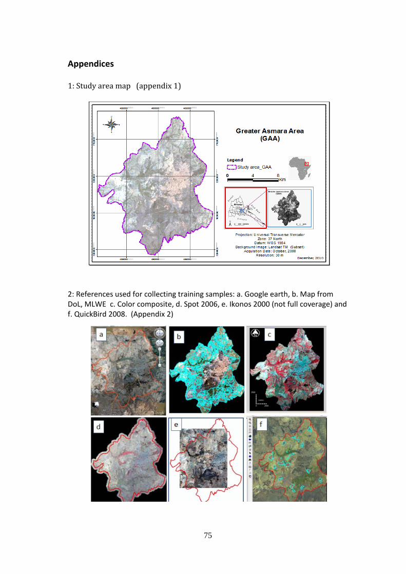
75

Appendices

1: Study area map (appendix 1)

2: References used for collecting training samples: a. Google earth, b. Map from DoL, MLWE c. Color composite, d. Spot 2006, e. Ikonos 2000 (not full coverage) and f. QuickBird 2008. (Appendix 2)

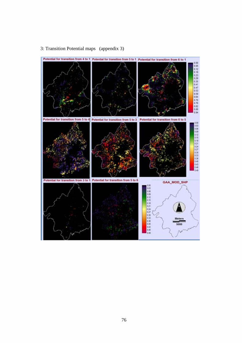
76

3: Transition Potential maps (appendix 3)

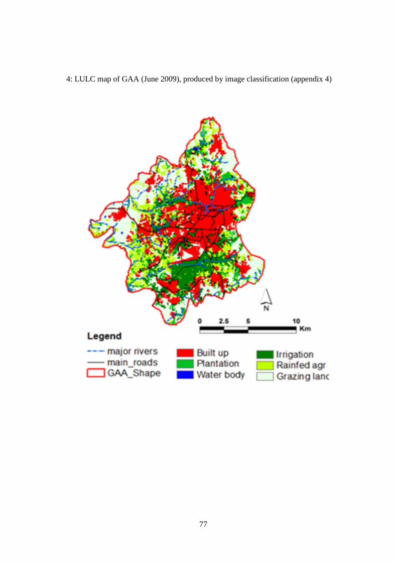
77

4: LULC map of GAA (June 2009), produced by image classification (appendix 4)

78

Declaration of originality I declare that, the submitted work is entirely my own and not of any other person

and that I have not used any other than permitted reference sources. All references

including citation of published and unpublished sources have been appropriately

acknowledged in the work. I further declare that the work has not been submitted

for the purpose of academic examination, either in its original or similar form,

anywhere else.

Münster, 28 February, 2011

Mussie Ghebretinsae Tewolde

---------------------------------------

79