Working Paper NO. 06-14 URBAN DENSITY AND THE RATE OF INVENTION

Gerald Carlino

Satyajit Chatterjee

Robert Hunt

Federal Reserve Bank of Philadelphia

First Draft: March 2004

This Draft August 2006

Supersedes Working Paper NO. 04-16/R

Working Paper NO. 06-14 URBAN DENSITY AND THE RATE OF INVENTION

Gerald Carlino

Satyajit Chatterjee

Robert Hunt

Federal Reserve Bank of Philadelphia

The authors thank Kristy Buzard for her excellent research assistance. We also thank Annette Fratantaro for her work on the Compustat variables and Jim Hirabayashi, of the U.S. Patent and Trademark Office, for his gracious response to our many questions. This paper has benefited from comments by Marcus Berliant, Mitchell Berlin, Jan Brueckner, Iain Cockburn, Gilles Duranton, J. Vernon Henderson, Andy Houghwout, Robert Inman, Sanghoon Lee, Loretta Mester, Leonard Nakamura, Giovanni Peri, Esteban Rossi-Hansberg, Albert Saiz, Rob Valetta, Kei-Mu Yi, and two anonymous referees. We alone are responsible for any remaining errors. The views expressed here are those of the authors and do not necessarily represent the views of the Federal Reserve Bank of Philadelphia or the Federal Reserve System

Working Paper NO. 04-16/R URBAN DENSITY AND THE RATE OF INVENTION

Gerald Carlino

Satyajit Chatterjee

Robert Hunt

Federal Reserve Bank of Philadelphia Economists, beginning with Alfred Marshall, have studied the significance of cities in the

production and exploitation of information externalities that, today, we call knowledge

spillovers. This paper presents robust evidence of those effects. We show that patent intensity—

the per capita invention rate—is positively related to the density of employment in the highly

urbanized portion of MAs. All else equal, a city with twice the employment density (jobs per

square mile) of another city will exhibit a patent intensity (patents per capita) that is 20 percent

higher. Patent intensity is maximized at an employment density of about 2,200 jobs per square

mile. A city with a more competitive market structure or one that is not too large (a population

less than 1 million) will also have a higher patent intensity. These findings confirm the widely

held view that the nation’s densest locations play an important role in creating the flow of ideas

that generate innovation and growth.

JEL Codes: O31 and R11

Keywords: Agglomeration economies, Knowledge spillovers, Urban density, Innovation, Patents

4

1. Introduction

With the emergence of endogenous growth theory in the 1980s, externalities associated

with knowledge spillovers have played a prominent role in thinking about sustained economic

growth of nations (Romer [44], Lucas [35] and Porter [42]). Lucas [35] argues that these

externalities are most likely manifested in cities since their dense concentration of people and

jobs is best suited to exploit them.

To date, economists have provided limited, but tantalizing, evidence on the existence and

importance of these spillovers. Jaffe, Trajtenberg, and Henderson [31] find that nearby inventors

have a much higher propensity to cite each others’ patents, suggesting that knowledge spillovers

are indeed localized. But their study does not explain how city characteristics, such as size and

local density, influence the production of these spillovers. Several authors find that patent

activity increases with metropolitan area size (Feldman and Audretsch [21] and O hUallachain

[41]). But these studies do not control for inputs into the innovation process, such as R&D, and

therefore cannot identify the external effects.

Ciccone and Hall [17] look at the relation between county employment density and

productivity at the state level. They find that a doubling of employment density in a county

results in about a 6 percent increase of average labor productivity. But why is density important

for productivity? We show that density is important in explaining innovative output, and this

may explain the pattern in productivity found by Ciccone and Hall [17].

In this paper, we explicitly examine the effects of employment density (jobs per square

mile), city size (total employment), and other characteristics on the rate of innovation across

metropolitan areas in the U.S. We use the average rate of patenting per capita—what we call

patent intensity—in a metropolitan area as a measure of innovative productivity in these areas.

We find a statistically significant relationship between patent intensity and employment density

5

in the highly urbanized portion of metropolitan areas. All else equal, patent intensity is about 20

percent higher in a metropolitan area with employment density that is twice that of another

metropolitan area. Since employment density doubles almost four times in our data set, the

implied gains in patent intensity are substantial.

Additionally, we have assembled a very rich data set, which permits us to test a number

of related hypotheses. For example, based on the criterion of maximizing patent intensity, we

find evidence of an optimal city size—about the size of Austin, TX, and optimal employment

density—about the density of Baltimore or Philadelphia. We find that cities with a more

competitive local market structure generate more patents per capita. We also find that our main

results are not sensitive to the measure of employment density used—we obtain similar

coefficients using all jobs or just certain categories of jobs most likely to consist of knowledge

workers.

2. The literature

Much of the theoretical literature on urban agglomeration economies has focused on

externalities in the production of goods and services rather than invention itself. Nevertheless,

the three mechanisms primarily explored in this literature are also relevant for the invention of

new goods and services: input sharing, matching, and knowledge spillovers.1 The first of these

points to the sharing of indivisible factors of production, or the benefits of increased variety of

differentiated inputs, that occurs in areas with a large number of final-goods producers (e.g.,

Helsely and Strange [28]). For example, Ciccone and Hall [17] show how density can give rise

to increasing returns in production due to the greater variety of intermediate products available in

1 These themes are developed in the excellent survey by Duranton and Puga [19]. Recent surveys of the empirical literature on agglomeration economies include Eberts and McMillen [20] and Rosenthal and Strange [45].

6

denser locations. They argue the positive correlation between employment density and

productivity implies that agglomeration economies dominate the congestion effects.2

A second theory argues that denser urban agglomerations improve the quality of matches

among firms and workers. Models of this sort include Wheeler [57], Helsley and Strange [27]

and Berliant, Reed, and Wang [11].3 In the latter, workers in dense locations are more selective

in their matches because the opportunity cost of waiting for a prospective partner is lower. That

is because, even though agents are more selective, on average they form matches more quickly.

As a result, the average output from matches is higher, and a higher share of the work force is

engaged in productive matches.

The third strand of theory argues that the geographic concentration of people and jobs in

cities facilitates the spread of tacit knowledge. While the exact mechanism is not well identified

in theory, the underlying idea articulated in Marshall [36] is that the geographic proximity

created by density facilitates the exchange of information among workers and firms. There does

appear to be some empirical evidence in favor of this view.4 But there can be too much density in

the sense that it may be harder to maintain trade secrets in more dense locations. This potential

for poaching may force firms to rely on patenting to a greater extent in dense areas.

While a full review of the empirical literature on the geographic extent of knowledge

spillovers is beyond the scope of this paper, we will touch on a few relevant papers.5 Rosenthal

and Strange [46] consider the importance of input sharing, matching, and knowledge spillovers

2 See also Sedgley and Elmslie [48]. 3 Similar testable implications can also be derived from Jovanovic and Rob [33], if one assumes either the meeting rate or their imitation parameter (m) is increasing in the density of workers. 4 See, for example, the interactions of semiconductor engineers in Silicon Valley as described in Saxenian [47]. 5 See Audretsch and Feldman [9] for a review of the literature on the geography of knowledge spillovers.

7

for manufacturing firms at the state, county, and zip code levels of geography. They find the

effects of knowledge spillovers on agglomeration of manufacturing firms tend to be quite

localized, influencing agglomeration only at the zip code level.6

Andersson, Burgess, and Lane [2] show that the correlation between workers’ skills

(education) and employers’ productivity (revenue per worker) at the establishment level is larger

in counties with higher population densities. They argue that this is evidence of superior

matching between workers and firms in more dense labor markets. Jaffe, Trajtenberg, and

Henderson [31], mentioned earlier, find that a new patent is five to 10 times more likely to cite

earlier patents from the same city than one would expect based on a control group of other

patents. Arzaghi and Henderson [8] find the density of advertising agencies in New York City

contributes to information spillovers that enhance productivity. Jaffe [32], Audretsch and

Feldman [10], and Anselin, Varga, and Acs [4] found evidence of localized knowledge spillovers

from university R&D to commercial innovation by private firms, even after controlling for the

location of industrial R&D. Many of these studies find that these externalities tend to be highly

localized even within a given metropolitan area.

Following Glaeser, et al. [24], much empirical research has focused on the effects of an

economy’s industrial structure on innovation and growth. Feldman and Audretsch [21], using

data from the U.S. Small Business Administration Innovation Data Base, found evidence

supporting the industrial diversity thesis of Jacobs [30]. Glaeser, et al. [24] studied employment

growth between 1956 and 1987 across specific industries within cities. They also found that

more industrially diversified metropolitan areas grew more rapidly.

6 Several other studies find that knowledge spillovers dissipate rapidly with distance. See, for example, Arzaghi and Henderson [8], Audretsch and Feldman [10]), and Keller [34].

8

In contrast, Henderson, Kuncoro, and Turner [29] examined employment growth rates

between 1970 and 1987 in eight manufacturing industries located in 224 cities. For five

traditional capital goods industries they found that employment growth in these sectors was

positively correlated with a high past concentration in the same industry, supporting the

industrial concentration, or Marshall-Arrow-Romer (MAR) view. They found evidence of both

MAR and Jacobs externalities for new high-tech industries.

Economists debate the effects of an area’s market structure on the rate of innovation and

growth. Chinitz [16] and Jacobs [30] argued that the rate of innovations is greater in cities with

competitive market structures. Glaeser, et al. [24] argue that the MAR view implies that local

monopoly may foster innovation because firms in such environments have fewer neighbors who

imitate them. The empirical literature tends to favors the Chinitz and Jacobs view over the MAR

view. Feldman and Audretsch [21] find that local competition is more conducive to innovative

activity than is local monopoly. Glaeser, et al.[24] find that local competition is more conducive

to city growth than is local monopoly.

3. Our data and regression strategy

Since data on innovations are not generally available at the local level, we use patents per

capita, what we call patent intensity, in a metropolitan area as our measure of innovative

productivity. This measure has its shortcomings, since some innovations are not patented and

patents differ enormously in their economic impact.7 Nonetheless, patents remain a useful

measure of the generation of ideas.

We regress patent intensity in a metropolitan area on measures of local employment

density, city size, and a variety of control variables. More specifically, the dependent variable in

7 For a general discussion on the use of patents as indicators, see Griliches [25].

9

our regressions is the log of patents per capita averaged over the period 1990-99.8 We use an

average over the 1990s to minimize any effects of year-to-year fluctuations in patent intensity,

which could be an issue in smaller metropolitan areas. To mitigate any bias induced by

endogeneity or reverse causation, the independent variables are at 1989-90, or roughly

beginning-of-the-period values. In section 6.2, we investigate these potential biases more closely

and find little, if any, effect on our results. Before presenting the exact specification, we will

describe the variables used in our regressions.

The sample consists of 280 metropolitan areas as defined in 1983. For brevity, we refer to

these as MAs. Included in this sample are 264 metropolitan statistical areas (MSAs) and primary

metropolitan statistical areas (PMSAs). To include as many patents as possible in our data set,

we group 25 component PMSAs into their corresponding nine consolidated metropolitan

statistical areas (CMSAs). We also group 21 separate MSAs into seven metropolitan areas.9 This

aggregation permits us to include an additional 9,000 patents (6.5 percent of the total) in our

regressions. Our main results are not affected if we drop these observations.

3.1 The patent data

Patents are assigned to metropolitan areas according to the residential address of the first

inventor named on the patent.10 We allocate patents to a county or metropolitan area when we

can identify a match to a unique county or metropolitan area. Patents that cannot be uniquely

matched are excluded from our data set. We can locate over 581,000 patents granted over the

1990-99 period to inventors living in the U.S. to either a unique county or MA, a match rate of

96 percent. Just over 534,000 (92 percent) of these patents are associated with an urban county.

8 For details on the construction of all our variables, see the Appendix. 9 See section A.2 of the Appendix for a list of MSAs that were combined. 10 In section 6. 1 we verify that our results are not sensitive to the choice of the first inventor’s address.

10

3.2 Land area

By definition, employment density is the number of jobs per square mile of land area.

Employment density varies enormously within metropolitan areas. It is typically highest in the

central business district (CBD) of an MA’s central city and generally falls off as we move away

from the CBD. But the vast majority of the land in MSA counties is in fact rural in nature, and

there is also considerable variation in the degree to which the counties surrounding a central city

are built out. For example, in the 1990 census only 12 percent of the 580,000 square miles of

land in MSA counties was categorized as urban in nature. The urban share of MSA land area

varied from less than 1 percent in Yuma, AZ to 65 percent in Stamford, CT.

We use a measure of land area that reflects the interaction of workers in labor markets

that are sufficiently dense to call urban—the urbanized area (UA) of cities.11 These are defined

as continuously built-up areas with a population of 50,000 or more, comprising at least one place

and the adjacent densely settled surrounding area with a population density of at least 1,000 per

square mile (U.S. Census Bureau, [54]). While UAs often cross county lines, we collected data

on urbanized area land in each county and then aggregated this number to the MA level.

3.3 Employment and density

For our purposes, the ideal measure of jobs and employment density would count only

those jobs located in the urbanized area of cities. Unfortunately, such data are generally

unavailable. For example, our preferred measure of employment is derived from the BLS survey

of payrolls. We also use these data in our measures of MA size and industrial composition.12 The

primary advantage of these data is that jobs are reported based on the place of work rather than

11 Mills and Hamilton [38] (p. 6) argue that urbanized areas correspond to the economist’s notion of urban areas. 12 All industry breakdowns in this paper are based on the 1987 Standard Industrial Classification system.

11

the place of residence. The disadvantage is that the data are reported at the county or MSA level,

but not for urbanized areas.

The Census Bureau reported a measure of employment in UAs in the 1990 census, but

this count is based on a worker’s place of residence, not his or her place of work. Most workers

live and work in the same UA, but a significant share of UA employment includes workers who

live outside the UA. For most UAs, a residency-based measure of employment will understate

employment density. The degree of understatement varies considerably across MAs.13

While we don’t have an ideal measure of employment density, we employ two

approximations that should bracket the ideal one. Both measures use the same denominator: the

sum of the land area lying in the urbanized area portion of the counties that compose an MA. In

the numerator of the first measure, we use the sum of all (establishment-based) employment

reported for the same counties. We refer to this measure as MA employment density. In the

numerator of the second measure, we use (residency-based) employment in the urbanized area

portion of the same counties, as reported in the 1990 census. We refer to this measure as UA

employment density.

To the extent that some metropolitan employment occurs outside of urbanized areas, our

MA employment density measure will overstate the actual density of jobs in the built-up portion

of MAs. We believe the extent of this overstatement is small and this measure is distinctly

superior to alternative measures. In 1990 urbanized areas accounted for 87 percent of the non-

rural land area of MSAs, 94 percent of the non-rural population, and 95 percent of non-rural

employment by place of residence. The latter statistic probably understates the share of jobs

13 The ratio of residency-based employment in UAs to establishment-based employment in the associated MAs in our data set is 0.58. The ratio varies from as little as 0.24 in Visalia, CA, to as high as 0.91 in Fort Lauderdale, FL.

12

located in urbanized areas because, as Glaeser and Kahn [23] show, MSA employment is more

tightly distributed around the central business district than are residents.

In any case, the most likely effect of such measurement error in our regressions would be

a negative bias in the coefficient on employment density. That is because we include in our

density measure jobs (in “rural” parts of the MA) less likely to be associated with innovation. In

that sense, any bias works against our hypothesis. To be conservative, however, we also ran our

regressions using our alternative measure, UA employment density. In addition, we report

regressions where we instrument for each density measure to better control for possible

endogeneity bias or measurement error.14

3.4 Local market structure and industrial diversification

To investigate the potential effects of local labor market structure on inventive output, we

construct a variable similar to one suggested in Glaeser, et al. [24]—the number of

establishments per worker in the metropolitan area. According to this definition, the higher this

ratio, the more competitive is the local labor market. This variable may capture more than a static

sense of industrial structure. If cities, or industries within a city, are experiencing considerable

entry or start-up activity, one would expect average establishment size to be smaller.

To explore the possible effects of local industrial diversification or specialization, we

construct a Herfindahl-Hirschman Index (HHI) of industry employment shares. Specifically, we

calculate the sum of the square of MA employment shares, in 1989, accounted for by seven one-

digit SIC industries, plus federal civilian jobs, state and local government jobs, and the

remainder. Higher values of this index for an MA imply that its economy is more highly

14 There is another source of potential downward bias in our coefficients. As noted earlier, a number of papers find that knowledge spillovers are highly localized, dissipating rapidly with distance from the source. Since we are using UAs or MAs as our unit of analysis, the coefficients on employment density we obtain may be underestimates.

13

specialized.

3.5 Local research inputs

Given that our regression relies on a cross section, it is important to take into account

factors that influence overall productivity in a city. We include many control variables for this

purpose. For example, it is well known that patent propensity varies significantly across

industries, so we include in our regressions the shares of total MA employment in manufacturing

and eight other industrial sectors.

We also control for the concentration of firms located in high technology industries. We

do this by calculating the share of patents obtained in an MA for the years 1980-89 owned by

firms in research-intensive industries.15 To control for variations in patent propensity by field of

technology, we computed the shares of patents obtained in each MA during 1980-89 categorized

into one of six technology groups as defined in Hall, Jaffe, and Trajtenberg [26].16

It is especially important to control for local inputs into the R&D process. To account for

the relative abundance of local human capital, our regressions include the share of the population

(over 25 years of age) with a college degree or more education in 1990. We also control for the

influence of having many nearby universities, a possible college town effect, by including the

ratio of college enrollment to population in the years 1987-89.

We include three other measures of research inputs in terms of their intensities.17 First,

we include in our regressions the sum of spending on R&D in science and engineering at local

colleges and universities divided by full-time enrollment at colleges and universities in the MA

15 See section A.1. of the Appendix for details on the construction of this variable. 16 Every patent in our data set was assigned to one of six broad categories (chemical, computer, medical, electrical, mechanical, and all other). We included the shares of the first five categories in our regressions. 17 Not surprisingly, the levels of these inputs are highly correlated with city size.

14

over the years 1987-89.18 We hope to capture the intensive margin—the R&D resources

available to potential researchers.19 Similarly, our regressions include the sum of federal funding

at government research laboratories in the MA divided by the number of federal civilian

employees in the MA (averaged over the period 1987-89). Finally, we include in our regressions

the number of private R&D facilities in 1989 divided by the number of private non-farm

establishments.20

3.6 Other control variables

Does a correlation between patent intensity and employment density reflect an actual

difference in inventive activity or, instead, differences in the way firms protect their inventions?

In her study of innovations in 19th century Britain, Moser [40] suggests that firms in industries

that rely less on patents tend to locate more closely together, while the opposite is true for firms

in industries that rely more on patents. In this paper, our regressions are based on aggregate

patenting per capita at the MA level, so we are unable to account for such patterns here. But

Moser also suggests that firms located in the most dense areas may rely more on patenting than

they otherwise would if it is more difficult to maintain trade secrets in such environments. In that

case, greater difficulty in maintaining secrecy, rather than spillovers, might explain our results.

To test the significance of this alternative explanation, we create an index of the

importance of trade secrecy that varies across metropolitan areas. We do this by weighting

industry-specific measures of the effectiveness of trade secrecy reported in Cohen, Nelson, and

18 Ideally, we would want to normalize by full-time S&E faculty or graduate students, but these cannot easily be assigned to particular campuses for a number of university systems that account for a significant portion of R&D. 19Anselin, Varga, and Acs [4] review studies examining localized spillovers from university R&D. Andersson, Quigley, and Wilhelmsson [3] find evidence that the expansion of the number of university-based researchers in a local labor market is positively associated with an increase in the number of patents granted in that area. 20 Over 1,800 private labs associated with the top 500 R&D performing corporations were geographically located using information contained in the Bowker Directory of American Research and Technology [13].

15

Walsh [18] by the industry shares reflected in the mix of private R&D facilities in every MA in

our data set. A higher value of this index for an MA implies that trade secrets are relatively more

effective for the mix of industries reflected in its R&D facilities. In addition, all of our

regressions control for the local mix of industries and technologies (see above).

We include a number of other control variables. We control for variations in

demographics by including the share of the population in 1990 that is of working age. We also

include the percent change in employment over the years 1980-89 as a control for the effects of

unobserved differences in local economic opportunities on inventive activity. We also include

seven dummy variables based on the BEA economic region in which the MA is located (the

Rocky Mountain region is omitted).

3.7 Our specification

Our main regression equation is simply:

14 202 2

1 2 3 4 5 15 16 216 16

35

22 23 24 25 26 27 28 i29

& + WAP +

i i i i i i g i i k ik ig k

i i i i i i i j ij ij

P C a D a D a E a E a COMP a INDSHR a HITECH a PATCLASS a PCTCOL

a CE a U a FEDLAB a R D a TS a EMPGT a a REGION ε

= =

=

= + + + + + + + + +

+ + + + + + +

∑ ∑

∑where:

Log of average patents per capita, 1990-99 in the i-th ;iP MA=

D MA job density in 1989 in density in 1990 in ;Log of or UA job i i i=

Log of 1989 level of employment in ;i iE MA=

= Log of the number of establishments in divided by total employment in , in 1989;i i iCOMP MA MA

= The share of employment in one-digit SIC industries in 1989 ;i iINDSHR MA

= Share of patents in during 1980-89 obtained by firms in R&D intensive industries; iiHITECH MA

= Share of patents obtained in during 1980-89, classified in one of five technological categories;

iikPATCLASS MA

16

= Percent of 1990 population over 25 with at least a college degree in ;i iPCTCOL MA

Ratio of the college enrollment to population in ;iCE i=

= University R&D spending per student, averaged for 1987-89 in ;i iU MA

Federal lab R&D per federal civilan job, averaged for 1987-89 in ;i iFEDLAB MA=

& Ratio of private labs to establishments in 1989 in ;iR D i=

iTS = Trade Secrets Index = The log of a weighted average of ratings of the effectiveness of trade secret protection in ;i

The percent change in employment in during the period 1980-89;i iEMPGT MA=

Share of the working age population in i;iWAP =

= dummy variables indicating in which of seven BEA regions is located;ij iREGION MA

is the random error term.iε

4. Main results

Table 1 shows the summary statistics for the variables used in the analysis. The average

number of patents per 10,000 of population obtained over the 1990s—our measure of patent

intensity—is about 2. San Jose stands out, with a patent intensity of 17. At the other end of the

distribution, the patent intensity for McAllen, TX, is only 0.07. Figure 1 demonstrates the

skewness of patent intensity across cities.

The urbanized land area of MAs varies considerably across cities: For Grand Forks it is

less than 15 square miles; for New York-Northeastern New Jersey, it exceeds 3,000 square

miles. Establishment-based employment in our MAs varies from 37,000 (Caspar, WY) to 9.6

million (New York-Northeastern New Jersey), while residency-based employment in the

urbanized areas of these MAs varies from 17,000 to 7.6 million. The mean of MA employment

density is 1,727 jobs per square mile while the mean of UA employment density is 987 jobs per

square mile. The latter varies from 263 jobs per square mile (Gadsden, AL) to 2,777 jobs per

17

square mile (Los Angeles-Long Beach).

Figure 2 plots the log of patent intensity against the log of MA employment density. A

moderate correlation (0.39) is clearly evident; there is a similar correlation between patent

intensity and UA employment density. In the regressions that follow, we explore how much of

this correlation remains after controlling for the many other factors that are likely to influence

inventive activity. The model is estimated using ordinary least squares in STATA, but we report

robust standard errors (White correction) to control for any heteroskedasticity.

4.1 Employment density and city size

Table 2 presents the main results of the paper. The regressions in columns 1 and 3 show

that, however measured, the effect of employment density on patent intensity is positive and

statistically significant.21 These coefficients can be interpreted as elasticities. All else equal,

patent intensity is about 17 percent to 20 percent higher in an MA that is twice as dense as

another MA. Employment density varies by more than 1,200 percent across the sample, so the

implied gains in the per capita invention rate are substantial.

Columns 2 and 4 report the results from regressions that add the square of our density

measures as independent variables. There is clear evidence of diminishing returns at very high

density levels. The optimal level—according to our MA employment density measure—is 2,190

jobs per square mile.22 That is about the 75th percentile of our data set, about the levels of

Baltimore (2,168) and Philadelphia (2,181). In section 5, we explore more narrow definitions of

employment density (e.g., scientists and engineers). We again find evidence of an optimal

density using these measures, but only at levels attained by about 10 percent of our sample.

21 Unless otherwise noted, t statistics are reported in parentheses. 22 The 95 percent confidence interval on this estimate is 1,418 - 3,384 jobs per square mile.

18

We now turn to the question of scale economies in the more traditional sense. Previous

research (Feldman and Audretsch [21], O hUallachain [41], and Bettencourt, Lobo and Strumsky

[12]) suggests that measures of innovation are positively related to metropolitan size

(population). Similarly, Ciccone and Hall [17] argue that the positive coefficient between

average labor productivity and employment density implies that agglomeration effects dominate

congestion effects. In their analysis, the elasticities for the agglomeration and congestion effects

are assumed to be constant. We relax that assumption here, allowing for diminishing returns to

scale and density as congestion effects become larger.

What do we find? When we include MA employment (in logs), but not its square, in our

regressions (not shown), the coefficient on this measure of city size is not statistically

significant.23 When we include the squared term, as we report in Table 2, the coefficients on

these variables are statistically significant. The implied optimal size, measured in terms of MA

employment, is about 500,000 jobs, about the 80th percentile of the size distribution in our data.24

If we assume a labor force participation rate of 66 percent, this corresponds to a population of

about 750,000, roughly the size of Austin, TX, or Raleigh-Durham, NC, in 1990. Thus, after

controlling for the effects of employment density, the benefits of urban scale are realized for

cities of moderate size. In fact, with the exception of San Jose, the top 5 percent of our

metropolitan areas ranked in terms of patent intensity had populations below 1 million in 1989.

4.2 Local competition

The regressions suggest that the rate of innovation is enhanced in more competitive local

environments characterized by many small firms, rather than in local economies dominated by a

23 The coefficient is 0.03 with a p value of about 0.40. 24 The 95 percent confidence interval for this estimate is 236,448 - 1,071,271.

19

few large firms. The coefficient on the number of establishments per employee is about 1.6 and

is precisely measured. The coefficient can be interpreted as an elasticity, since the variable is

included in logs in our regression. The effect is economically significant, as this ratio more than

doubles across our sample. This result is consistent with the views of Chinitz [16], Feldman and

Audretsch [21], Glaeser, et al. [24], and Jacobs [30] that competitive local labor markets

facilitate innovation. We are not able to determine whether this results from static (market

structure) or dynamic (firm entry) effects, or both.

4.3 Industrial mix and specialization

Patent activity varies enormously across industries. As expected, the manufacturing share

of MA employment is positively related to local patent intensity. All else equal, a 10 percent

increase in the manufacturing share of employment is associated with a 3 percent increase in

patent intensity. Conversely, a 10 percent increase in the state and local government share of

employment is associated with a 4.5 percent decrease in patent intensity.

If knowledge spillovers occur largely within industries, specialized cities may be more

efficient producers of inventions. On the other hand, if important spillovers are generated across

industries, perhaps more industrially diverse cities may be more efficient innovators. To test for

such effects, we constructed a commonly used measure of concentration, an HHI of industry

employment shares (see section 3). When we include this variable in our regressions (not

shown), the estimated coefficient is never statistically significant.25 We also constructed a

measure of technological specialization using our technology share controls. When we included

this variable in our regressions (not shown), the estimated coefficient was negative, but not

significant (p = 0.13). In short, our results suggest that while the mix of industries is obviously

25 When all our employment shares are also included, the coefficient on HHI is essentially zero. If we include only the manufacturing share of employment, the coefficient on HHI is negative, but not significant.

20

important in explaining the overall patent intensity of cities, the concentration or dispersion of

economic activity across industries does not appear to have an independent effect.

4.4 Local research inputs

The results reported in Table 2 clearly show that local research inputs are important to

explaining the variation in patent intensity across MAs. The coefficients on our controls for

research-intensive industries and the controls for most technology fields are statistically

significant and precisely measured. These variables capture characteristics relevant to patent

intensity that are not fully explained by local industry mix and structure. The largest elasticities,

evaluated at the mean, are for chemical inventions (0.30), mechanical inventions (0.24),

computers (0.19), and high-technology industries (0.16).

By far the most powerful effect is generated by human capital (the share of the adult

population with at least a college degree). A 10 percent increase in this ratio is associated with an

8.6 percent increase in patents per capita. We also included a variable to capture the relative size

of higher education in a metropolitan area—the ratio of college enrollment to population. The

coefficient on this variable (not shown) is not significant in our regressions, suggesting there is

no separate college town effect on the local invention rate.26

Our other controls for local research intensities include the ratio of academic R&D in

science and engineering to student enrollment (in 1987-89), federal lab R&D spending per

federal civilian employee (in 1987-89), and the number of private R&D labs per 1,000

establishments (1989). All of these variables have a positive impact on the rate of patenting, but

the implied elasticities are relatively small. For example, a 10 percent increase in private R&D

intensity is associated with only a 1 percent increase in patent intensity. The elasticity for

26 In other regressions we included the log of the number of colleges and universities in the MA. But the coefficient on this variable is never statistically significant.

21

academic R&D intensity is slightly smaller (.08). Still, these effects are economically significant

because there is considerable variation in academic and private R&D intensity in our data (see

Table 1).

Agrawal and Cockburn [1] argue that local academic R&D is likely more productive, in

terms of its contribution to additional patents, in the presence of a large research-intensive firm

located nearby—the anchor tenant hypothesis. Taking this effect into account, they report a

significant positive correlation between local patents and academic publications in the fields of

medical imaging, neural networks, and signal processing. We looked for a more general

interaction—do cities with a relative abundance of academic and private R&D enjoy a

disproportionately high patent intensity? We tested for this by interacting our measures of

academic and private R&D intensity and including them in our regressions (not shown). We

were surprised to find a significant, but negative coefficient (-0.13) on this interaction term.27

There does appear to be some degree of substitution between local academic and private R&D

investments, but the effect is quite small—the implied elasticity at the mean is -0.03.28

4.5 Trade secret protection

Recall that we constructed an index of the efficacy of trade secret protection among firms

located in an MA. If the estimated coefficient on this variable is negative, we might be concerned

that firms are substituting patents for trade secret protection in dense areas because the former

are relatively more effective in such environments. We find, instead, the estimated coefficient is

positive but insignificant at standard confidence levels. This is consistent with Cohen, Nelson,

27 The p value is 0.026. The coefficients on the academic and private R&D variables remain significant; in fact they increase by more than the estimated coefficient on the interaction (but the changes in these coefficients are not statistically significant). The other regression coefficients hardly change. Note that the correlation between the private and academic R&D intensities in our data is only 0.17. 28 We also interacted the R&D intensity of private and government labs, but found no significant effects.

22

and Walsh [18], who find a positive correlation in firms’ rating of the effectiveness of trade

secrecy and patent protection. It is also consistent with the result in Fosfuri and Rønde [22], who

find that trade secret protection stimulates clustering in a model of firm location in the presence

of information spillovers. In any case, city size and employment density remain important in

explaining patent intensity even after controlling for an industry’s reliance on trade secret

protection.

Helsley and Strange [27] argue that knowledge transfers between agents may arise

through a form of barter in the absence of established property rights in the underlying ideas.

They argue this barter process may be more effective in smaller metropolitan areas where

anonymity is harder to maintain. In larger MAs, informal exchange (or cooperation) may become

unsustainable and agents are forced to patent their ideas before they can exchange them for

anything valuable. To test this hypothesis, we interacted our trade secrets variable with city size

and, alternatively, with employment density (not shown), but we did not find any statistically

significant interactions. These results suggest that the phenomenon we are measuring is real, i.e.,

there really are more inventions.

4.6 Employment growth and other control variables

The coefficient on employment growth in the previous decade (not shown) is positive but

not statistically significant in our main regressions (it is sometimes significant in other

specifications).29 This is true even when we drop our establishments per worker variable, which

might also pick up variations in city or industry dynamics. Our demographic control, the share of

the population of working age (not shown), is always positive but is statistically significant in

only some regressions. The estimated coefficients on two of the seven BEA region dummies (not

29 It varies from about 0.28 to about 0.34 in the regressions reported in Table 2.

23

shown) are statistically significant. MAs located in the New England and Southwest regions had

lower patent intensities. Overall, it appears that our controls do a good job of accounting for the

other factors that contribute to innovation in cities.

5. The density of knowledge workers

To this point, our measures of employment density reflect the entire workforce of the

MA. Not all of these jobs are directly involved in the process of inventing new products or

processes. So it is reasonable to ask whether it would be better to instead focus on a measure of

occupations consisting of the knowledge workers in an MA.

We avoid doing this in our main regressions (Table 2) for several reasons. First, it is not

obvious what the appropriate set of occupations should be. Second, a substantial amount of

invention occurs when users of a product or process modify it to suit their particular needs

(Morrison, Roberts, and Von Hippel [39]). These users may not fall into the occupations we

might include in the class of knowledge workers. Third, our industry, technology, and human

capital controls ought to absorb most of the effect of the unobserved variation in the composition

of the workforce. If our general measures impart a bias, then the bias should work against us.

Nevertheless, we re-estimate our specifications using two more narrow measures of

employment density. The first includes only those jobs falling into the Census Bureau’s

classification of professional specialty occupations. This grouping includes engineers, scientists,

social scientists, doctors, and other health professionals. But it also includes teachers, lawyers,

artists, and athletes. The second includes only scientists and engineers living in the urbanized

area in 1990. Both of these are residency-based measures of employment in 1990.

In Table 3, we report results using each measure in our primary specifications. In the first

and third columns of the table, we show that the estimated coefficient on employment density is

24

about 0.22 and is measured very precisely (p < 0.01). The estimated coefficients on most other

variables change only slightly. The estimated coefficient on our human capital measure falls a

bit, especially when we use the density of scientists and engineers in our regressions. The

estimated coefficients on manufacturing employment share are also a bit smaller.

We also constructed a density measure counting only jobs that do not fall into the Census

Bureau’s professional and specialty classification. This measure explicitly excludes scientists,

engineers, medical professionals, and college professors. If we include only this measure of

density in our regression (not shown), the estimated coefficient is 0.19 and is statistically

significant (p < 0.05). If we include both density measures in the regression (not shown),

professional specialty occupations and the other jobs, the coefficient on the latter measure is

negative but insignificant, while the coefficient on the former measure rises and remains

significant. We conclude that while much of the effect of density on patent intensity is

concentrated in these more narrow categories of jobs, using our general measures of job density

does not bias our results.

Columns 2 and 4 of Table 3 verify there are diminishing returns to employment density

even when using these measures. The optimal density of professional specialists is 320 per

square mile, the 88th percentile of our sample. The optimal density of scientists and engineers is

57 per square mile, the 92nd percentile of our sample. Thus, in our data, relatively few MAs

exhaust the returns to scale associated with the density of these jobs. The estimated optimal

scale, measured in terms of population, in these regressions falls to about 650,000 to 700,000.

6. Testing for robustness

In this section, we examine a number of factors that might potentially affect our results.

We consider alternative specifications, reverse causation and endogeneity bias, and spatial

25

dependence. None of the main results are affected after controlling for these issues.

6.1 Alternative specifications

To this point, we have associated inventions with MAs on the basis of the home address

of the first inventor listed on the patent. One might wonder about how the first inventor is

selected and whether this process might affect our regression results. For example, suppose a

multinational company patents an invention developed by researchers working in separate labs in

different cities or even countries.

For a variety of reasons, we do not believe such concerns should significantly affect our

results. About 49 percent of our patents have only one inventor. Among the other patents, only

2.6 percent involve inventors living in different countries, and only a third of these report a first

inventor living in the U.S. Among the patents where the first two inventors live in an American

city, nearly 70 percent live in the same MA. When inventors do live in separate MAs, they tend

to live far apart. The average distance is 560 miles.

Table 4 reports two sets of regressions. The first two columns of Table 4 are based on the

same specification reported in columns 1 and 3 of Table 2, except we add 3 new variables to the

regressions: the share of the MA’s patents with a second inventor residing in another MA, the

log of the average distance between inventors’ MAs for those patents, and the square of this

distance. The coefficient on each of these variables is statistically significant. All else equal, the

higher the share of an MA’s patents with a second inventor living in another MA, the lower is

the MA’s patent intensity. This is not surprising as it is likely that firms with a more

decentralized workforce are also likely to have a more even spatial distribution of patents. The

estimated coefficients on our density measures are somewhat larger than reported in Table 2,

while the estimated optimal city size falls to about 500,000.

26

Somewhat surprisingly, the coefficient on the average distance between inventors’ MAs

is positive (the coefficient on the square of distance is negative). Conditional on relying on a

distant co-inventor, the optimal distance between MAs is 270-330 miles, depending on the

density measure used in the regression. These results suggest that inventors may be taking

advantage of differentiated knowledge available in other MAs, a finding consistent with the

intuition of Berliant, Reed, and Wang [11].

In Columns 3 and 4 of Table 4 we report the findings when we repeat the specification

used in columns 1 and 3 of Table 2, except that the observations are based on the address of the

second inventor on the patents. The coefficients on the density and size variables are statistically

significant and take the same sign as in Table 2. Similar results (not shown) are obtained when

we use any of our other density measures. We conclude that our findings are not sensitive to the

choice of the first inventor’s address in our analysis.

6.2 Reverse causation, endogeneity, and consumption amenities

Our regressions estimate the effects of employment density and city size on patent

intensity. In this section, we directly address the possibility of reverse causation—patent

intensity might affect city size, employment density, or both.

We begin with simple Granger causality tests (not shown). In the forward regression, we

regress patent intensity in the 1990s on patent intensity in 1975-79, and MA employment density

in 1989 (all in log form). The coefficient on the last of these variables is 0.43 and significant at

the 1 percent level. In the reverse regression, we regress MA employment density over the 1990s

on employment density in 1989 and patent intensity in 1975-79 (all in log form). The coefficient

on the lag of patent intensity is significant at the 1 percent level, but the coefficient is also very

small (-0.01). While we reject the hypothesis of no reverse causation, the estimated effect is

27

more than an order of magnitude smaller than the relationships estimated in our main

regressions.

Even though all of our independent variables are significantly lagged, one may still be

concerned about the possibility of endogeneity and a resulting bias in the estimated coefficients.

A related concern is that a correlation between patent intensity and employment density might

occur if highly productive (i.e., inventive) workers are attracted to MAs by consumption

amenities (e.g., variety) not adequately controlled for in our regressions and which are not

already reflected in our human capital variables.30 To address these possibilities, we perform

instrumental variables (2SLS) regressions and examine Hausman tests for endogeneity bias. We

instrument for employment density, employment, and its square.

In addition to the other right-hand-side variables in our main regressions, we include as

instruments a variety of weather and topographic variables. The existence of a significant

correlation between such variables and density has been documented in other work (Rappaport

[43]). We also include deep lags of MA urbanized land area (1980) and employment (1970), in

logs, and the square of these variables. Finally, to address the possibility that other consumption

amenities explain our results, we include as instruments the number of museums, restaurants,

violent crimes, and property crimes in 1989, each expressed in per capita terms.31

Our weather and topography variables are derived from the USDA’s Economic Research

Service Natural Amenity Scale.32 These data are reported at the county level and include mean

hours of sunlight in January, mean temperature in January and July, and the percent of county

30 While it is possible that such amenities may attract more population, and thus employees, it does not explain the negative correlation between patent intensity and urbanized land area in a regression (not shown) controlling for employment and our other control variables. 31 These data are derived from County Business Patterns. 32 For more information, see http://www.ers.usda.gov/data/naturalamenities and McGranahan [37]).

28

area covered by water. These variables are aggregated to MAs, weighting by county land area.33

We also construct dummy variables that reflect the presence of five topographic features in MA

counties: plains, tablelands, open hills and mountains, hills and mountains, and plains with hills

and mountains.

The F statistic in each of the first stage regressions is at least 24 or higher, suggesting that

our instruments are strong. Columns 1 and 3 of Table 5 report OLS estimates for the same

sample of cities we can estimate using our instruments (we lose six observations owing to

missing variables). Columns 2 and 4 report the coefficients from the instrumental variables (IV)

regressions. The estimated coefficients on MA employment density fall somewhat relative to

OLS in the IV regression but the opposite pattern is observed when we examine the regressions

with UA employment density. This is what we would expect when we correct for measurement

error in these two variables (see section III). In any case, Hausman tests do not identify any

systematic differences between the OLS and IV coefficients in these regressions.

We also performed IV regressions using an even deeper lag of urbanized land area (1970)

as an instrument (not shown). The estimated coefficients on employment density and city size

are slightly larger than the comparable OLS estimates, but they are no longer statistically

significant.34 Again, Hausman tests do not identify any systematic differences between the IV

and OLS estimates. We conclude that any remaining endogeneity in our regressions is unlikely

to explain our main results.

6.3 Spatial dependence

There is a very high degree of spatial inequality in the distribution of patent activity.

33 We also include the water area of MA counties, in square miles, as reported by the Census Bureau for 1990. 34 In these regressions, the p values for the coefficients on MA and UA employment density, respectively, are 0.12 and 0.16. The sample size in these regressions is only 227.

29

Patenting tends to be highly concentrated in the metropolitan areas of the northeast corridor,

around the Research Triangle in North Carolina, and in California’s Silicon Valley. Even though

the coefficients on our regional dummy variables are typically insignificant, this clustering of

innovative activity suggests there could be strong spatial dependence at a more localized level

and, if so, it should be controlled for in our empirical analysis.

The conjecture, then, is that patent intensity in one MA may be highly correlated with

patent intensity in nearby MAs. The consequences of spatial autocorrelation are the same as

those associated with serial correlation and heteroskedasticity: When the error terms across MAs

in our sample are correlated, OLS estimation is unbiased but inefficient. However, if the spatial

correlation is due to the direct influence of neighboring MAs, OLS estimation is biased and

inefficient (Anselin [7]).

The literature suggests two approaches to dealing with spatial dependence. In the first

approach, spatial dependence is modeled as a spatial autoregressive process in the error term:

2(0, )W

Nε λ ε µ

µ σ

= +

∼

where is the spatial autoregressive parameter and is the uncorrelated error term.λ µ W is a

spatial weighting matrix where nonzero off-diagonal elements represent the strength of the

potential interaction between the ith and jth MAs. We use the inverse of the square of the

geographic distance between MAs to fill in the off-diagonal elements of W . The null hypothesis

of no spatial error dependence is 0 : 0H λ = .

The second approach models the spatial dependence in patenting activity via a spatially

“lagged” dependent variable:

P WP Xρ β ε= + +

30

where P is an Nx1 vector and N is the number of locations in our study; ρ is the autoregressive

parameter (a scalar); W is the NxN spatial weight matrix described above; X is an NxK matrix of

other explanatory variables from before; and ε is the Nx1 random error term. The null

hypothesis of no spatial lag is 0 : 0H ρ = .

Following Anselin and Hudak [5], we perform three tests for spatial autocorrelated

errors: Moran’s I test, the Lagrange multiplier (LM) test, and a robust Lagrange multiplier test

(robust LM). We also perform two tests for the spatial lag model (LM test and a robust LM test).

The Moran’s I test is normally distributed, while the LM tests are distributed 2χ with k and one

degree of freedom, respectively.

We estimate each of the specifications previously reported in Table 2 using these various

tests for spatial dependence. The results are summarized in Table 6. The null hypothesis of zero

spatial lag cannot be rejected in any specification. The results for spatial error are somewhat

more ambiguous. The null hypothesis is clearly rejected according to the Moran’s I test, but not

according to the LM and robust LM tests. Anselin [6] reports that the Lagrange multiplier tests

are more robust than the Moran’s I test under Monte Carlo simulations, which suggests that

spatial error is unlikely to be an issue for our specifications.

Nevertheless, we re-estimate each specification reported in Table 2, incorporating a

correction for either spatial error or spatial lag. Table 7 presents the results for the specifications

used in columns 1 and 3 of Table 2.35 As expected, we did not find any instances of a significant

spatial error or spatial lag coefficient. The primary effect of using maximum likelihood

procedures is that most of the coefficients are estimated more precisely.

35 These estimates were obtained using the Spatreg procedure in STATA. The results for the specifications reported in columns 2 and 4 of Table 2 are nearly identical to the OLS results.

31

7. Conclusion

Patent intensity—the per capita invention rate—is positively related to the density of

employment in the highly urbanized portion of MAs. All else equal, the number of inventions

per person is about 20 percent greater in an MA with a local economy that is twice as dense as

another MA. Since local employment density doubles more than four times in the sample, the

implied gains in patents per capita due to urban density are substantial. In short, we find

empirical evidence consistent with a theoretical micro foundation of endogenous growth. In

addition, we find evidence of increasing returns to scale in the invention process, but holding

density constant, these returns are exhausted at a modest city size—certainly below 1 million in

population. Similarly, we find evidence of diminishing returns to density, but only at levels

attained by a quarter of our sample.36

Our results also support theories that suggest that more competitive local market

structures are more conducive to innovation. We find that industrial and technology mix are

important in explaining the variation in patent intensity across cities, but we found no significant

effects for our measures of industrial or technological specialization. We found that local R&D

inputs, especially human capital, contribute to higher patent intensities and there is evidence of a

very modest substitution effect between academic and private R&D intensity. Variations in the

reliance of a city’s industries on trade secret protection did not have a significant effect in our

regressions.

In the empirical work we have been careful in our definition of the unit of analysis and

the inclusion of control variables that reflect the available resources (e.g. R&D, human capital,

etc.) that are relevant to the local output of innovations. Thus we believe our coefficients on city

36 Diminishing returns to density sets in much later in our sample (about the 90th percentile) if we instead use only scientists and engineers in our density measure.

32

size and density reflect effects that are external to the firm, but not to the city itself. On the other

hand, our regressions are not sufficient to identify a particular mechanism that explains why

these externalities are important. We have suggested a few possibilities, such as better matches

between firms and workers or easier transmission of tacit knowledge, but our technique cannot

distinguish among them. In order to do so, we require more refined theories and yet more data.

To investigate these questions more precisely, one might examine an additional direction

of cross-sectional variation, that is, differences across industries. In particular, this would allow

one to test the significance of urbanization economies (city size) and localization economies (the

local size of the industry).37 A stronger approach is to focus on firms, the source of most of the

innovations in our data, and to investigate the contribution of city characteristics to the

productivity of the research efforts located in them. These are topics of our ongoing research.

APPENDIX A

A.1. Patent data

Our patent data are derived from data sets furnished by the Technology Forecasting and Assessment Branch of the U.S. Patent and Trademark Office. These include the US Patent Inventor File 1977-99: All Grants; 75-76 Utility Patents Only and the PATSIC99 file.

We assemble the home address information of the first inventor named on each patent from the inventor’s file. We began with 1,198,376 patents granted to inventors with an American address over the years 1975-1999. We assigned a state-county FIPS code for each patent by matching address information against the 1998 vintage of NIST’s FIPS55 place names data set. We obtained unique ZIP code-county and place name-county matches for 81 percent of the patents. For another 8.5 percent of the patents, we could not initially identify a unique county for the inventor but we could identify a unique metropolitan area. Another 6.6 percent of patents were geographically located via matches against the location of an R&D lab of the firm owning the patent and manual searches.

In all 1,155,133 patents were matched to a county or an MA, while 43,243 were not. Of those patents that were successfully placed in an MSA, 581,001 were granted between 1990 and 1999 (inclusive); 46,647 were located outside an MSA. That leaves 534,354 patents in MAs that were used to construct the patent variable.

37 For preliminary work in this direction see Carlino and Hunt [15].

33

The field of technology dummies (medical, chemical, computer, electrical, and mechanical) are constructed by matching the primary classification number of each of our patents to one of the sets of classifications contained in Appendix 1 of Hall, Jaffe, and Trajtenberg [26].

To construct the high-technology industry patent share, we match our patent numbers to those contained in the NBER Patent Citations Data File, and obtain the CUSIP of the firm that was initially assigned the patent. We associate this firm, using its CUSIP, to the SIC assigned to it in the 1999 vintage of Standard and Poor’s Compustat. High tech industry patents are those associated with firms that have a three digit SIC code in one of the R&D intensive industries identified in Office of Technology Policy [55]. We calculate the high tech share of patents in a city by dividing this number by the number of all patents in the city that we can match to a firm in the NBER Patent Citations Data File. In total, we were able to match over 141,000 urban patents (41percent of the total) granted in the 1980s to firms in the 1999 vintage of Compustat.

A.2. Our definition of metropolitan areas

Our MA definitions are based primarily on MSA definitions defined by the Office of Management and Budget in 1983 (http://www.census.gov/population/estimates/metro-city/83mfips.txt). Several adjustments are made:

- The six MSAs in Puerto Rico are removed.

- New England County Metropolitan Areas (NECMAs) are used as our MAs in New England.

- The Bureau of Economic Analysis (BEA) uses its own set of county-equivalent codes to tabulate data for independent cities and their surrounding counties together. For all data from the Regional Economic Information System (REIS), data for our MAs are built up including these independent cities.

- Nine Consolidated Metropolitan Statistical Areas (CMSAs) are employed instead of their 25 component MSAs: Chicago, IL-IN-WI; Cincinnati-Hamilton, OH-KY-IN; Cleveland-Akron-Lorain, OH; Dallas-Fort Worth, TX; Houston-Galveston-Brazoria, TX; Kansas City, KS-MO; Portland-Vancouver, OR-WA; Seattle-Tacoma, WA; and St. Louis- East St. Louis- Alton, IL-MO.

- Seven ad hoc metropolitan areas were also created: Denver-Boulder-Greeley (Boulder-Longmont, CO PMSA; Denver, CO PMSA; & Greeley, CO MSA); Greenville-Anderson (Anderson, SC MSA and Greenville-Spartanburg, SC MSA); Los Angeles-Anaheim (Anaheim-Santa Ana, CA PMSA and Los Angeles-Long Beach, CA PMSA); Midland-Odessa (Midland, TX MSA and Odessa, TX MSA); New York-Northern New Jersey (Bergen-Passaic, Jersey City, Middlesex-Somerset-Hunterdon, Monmouth-Ocean, Nassau-Suffolk, New York, Newark, Orange County, New York); San Francisco-Oakland (Oakland, CA PMSA and San Francisco, CA PMSA); and Sarasota-Bradenton (Bradenton, FL MSA and Sarasota, FL MSA).

We used these definitions for certain cities rather than the underlying MSAs because two or more cities shared a common border and we could not always assign some patents (a few thousand) to an MSA with certainty (see Patent Data above). If we used the underlying MSAs, we would either have to discard these patents or take the chance that the error rate in assigning patents to cities might vary systematically across cities. The methodology used in USPTO [56] assigns equal shares of patents to counties with common place names when a patent cannot be

34

matched to a unique county. This too might imply a higher error rate in assigning patents when MSAs are close to each other.

We compared our MSA patent counts to those reported in USPTO [56] and found them to be extremely close, except for a few instances. In some cases two or more MSAs were in close proximity (e.g., Dallas and Fort Worth). In a few others, the place name of the inventor’s address was common to more than one county, regardless of distance. The PTO algorithm divided those patents equally across those counties.

Our definition of metropolitan areas or the manner of allocating patents to MSAs does not significantly influence our results. In an earlier version of this paper (Carlino, Chatterjee, and Hunt [14]) we estimated the relationship between patent intensity and employment density using a data set of 296 MSAs and PMSAs as defined by OMB in 1983 and using patent counts built up from the data contained in USPTO [56]. The results were qualitatively the same as those reported here, although the estimated coefficients were somewhat larger.

A.2.1. Missing data

Four MSAs are dropped in the analysis because of missing data. One MSA (Enid, OK) does not have a corresponding urbanized area. Owing to disclosure limitations, a Herfindahl index of industry employment shares cannot be calculated for Atlantic City, NJ, and Tallahassee, FL. In addition, manufacturing employment is not available in 1989 for Columbus, GA-AL.

A.3. Geographic variables

Urbanized Area land area for every county was obtained from Table 34 of Census Bureau [51]. We also obtained comparable measures for urbanized areas defined in 1980 and 1970 from Census Bureau [49], [50].

There are a few instances where a county includes land area associated with more than one urbanized area. For example, portions of Bucks County, PA, are associated with the Philadelphia and Trenton urbanized areas. To be consistent with our other county-based measures, we attribute this land area (and associated employment) to the MA associated with that county (e.g., Philadelphia).

The weather and topography instrumental variables are based on the USDA’s Natural Amenity Scale project (http://www.ers.usda.gov/data/naturalamenities). The data are reported at county level, which we aggregate, based on county land area, to MSAs. We use the variables indicating, for the years 1941-1970, mean hours of sunlight and temperature in January, mean temperature in July, the percent of land area covered by surface water, and five dummy variables for the presence of a particular type of geography (plains, tablelands, open hills and mountains, hills and mountains, and plains with hills and mountains) built up from a finer gradation in the ERS data. We also included as an instrument the amount of MA area covered by water n 1990. Those data were obtained from a county level tabulation reported in the Census Bureau’s Gazeteer (http://www.census.gov/geo/www/gazetteer/gazette.html).

A.4. Economic and demographic variables

Our primary employment data are county-level values reported in the BEA’s REIS database and aggregated to the MA level. We use the 1999 vintage of these data. The data are derived from the BLS Covered Employment and Wages Program (ES-202), which represents the

35

average annual number of full- and part-time jobs held by all workers who are covered by unemployment insurance. Industry breakdowns are based on 1987 SIC definitions.

Our measures of residency-based employment in 1990 were obtained from the Census Bureau web site (www.americanfactfinder.com). Those data are derived from the STF3 (5 percent sample) tape. A separate count was obtained for every county that includes an urbanized area. These are aggregated to MAs in the same manner as our other variables.

Our counts of employment for professional specialty occupations are derived from the 1990 census (STF3). This is a residency-based count, but here we include all residents in the counties making up an MA, not just residents in the urbanized area portion of those counties. The occupation codes for this category of jobs are codes 043-202 in the 1990 Census Occupation Classification System.

Our counts of scientists and engineers are residency-based measures of workers in these occupations living in urbanized areas as reported in Table 34 of Census Bureau [53]. We aggregated these counts to be consistent with our MA definitions.

The shares of MSA land area, population, and employment contained in urbanized areas discussed in section 3.3 are derived from Tables 48, 50-51 of Census Bureau [51] and Table 33 of Census Bureau [52] and Census Bureau [53].

The Herfindahl-Hirschman Index (HHI) is calculated for 1989 and includes employment for ten industrial sectors. These include Construction, Manufacturing, Transportation and Public Utilities, Wholesale Trade, Retail Trade, Finance, Insurance, and Real Estate, Services, Civilian Federal Government, State and Local Government, and a category, other, that consists primarily of employment in the military, agriculture, and mining. The HHI is calculated at the MA level. Wherever county data are missing for 1989, either data from the previous or following year are used or MSA-level data are substituted when appropriate.

The percentage of population with a college degree or more education is derived from the 1990 Census American Fact Finder. Because these are MSA-level data, it was necessary to create a weighted average of component MSAs for the special CMSAs we created; this was done using 1990 Census Bureau mid-year population estimates aggregated from county level to MSA. The population data were also used to calculate our measure of patents per capita.

Our instrumental variables include a measure of the number of restaurants and museums and crimes in 1989. These are derived from county-level data, as reported in County Business Patterns, and aggregated to the MA level. They are converted to intensities by dividing by population in 1989.

A.5. Research and development variables

The amount of academic R&D in each MSA is derived from the National Science Foundation’s (NSF) “Academic Science and Engineering: R&D Expenditures,” as archived in the WebCaspar search engine at the NSF web site. Expenditures are averaged over the period 1987-89 and are normalized by the total fall enrollment as reported in the Integrated Postsecondary Education Data System assembled by the National Center for Education Statistics and archived on WebCaspar. S&E expenditures reported for a number of university systems were also allocated to particular campuses using advanced S&E degrees granted by those campuses. Expenditures are built up from counties according to our MA definitions.

36

Data on the location and resources of the Federally Funded Research and Development Centers were provided to us by Ronald Meeks of the National Science Foundation.

Data on private R&D facilities were extracted from the 1989 edition of the Bowker Directory of American Research and Technology [13]. They are matched to the SIC of the parent company using the 1999 vintage of Compustat.

A.6. Trade secrecy index

We assigned the industry-specific effectiveness rating in Table 1 of Cohen, Nelson, and Walsh [18] to two-digit or three-digit SIC industries. These ratings are a categorical response to a question that asks for the proportion of product innovations for which trade secrets are effective in preserving the resulting profits. For each MA, we compute a weighted average of the industry ratings using as weights the shares of all private R&D facilities in the MA contained in those industries.

References

[1] Agrawal, A., and I. Cockburn, The anchor tenant hypothesis: Exploring the role of large, local, R&D-intensive firms in regional innovation systems, International Journal of Industrial Organization 21 (2003) 1217-1433.

[2] F. Andersson, S.M. Burgess, J. Lane, Cities, matching and productivity gains of agglomeration, Discussion Paper No. 4598, CEPR, 2004.

[3] R. Andersson, R. J. Quigley, M. Wilhelmsson, Higher education, localization and innovation: Evidence from a natural experiment, mimeo, University of California at Berkeley, 2005.

[4] L. Anselin, A.Varga, Z. Acs, Local geographic spillovers between university and high technology innovations, Journal of Urban Economics 42 (1997) 442-448.

[5] L. Anselin, S. Hudak, Spatial econometrics in practice: A review of software options, Regional Science and Urban Economics 72 (1992) 509-536.

[6] L. Anselin, Some robust approaches to testing and estimation in spatial econometrics, Regional Science and Urban Economics 20 (1990) 141-163.

[7] L. Anselin, Spatial Econometrics: Methods and Models, Kluwer Academic Publishers, Boston, 1988.

[8] A. Arzaghi, J.V. Henderson, Networking off Madison Avenue, Unpublished manuscript, 2005.

[9] D.B. Audretsch, M.P. Feldman, Knowledge spillovers and the geography of innovation, in: J.V. Henderson, J-F. Thisse (Eds.), Handbook of Urban and Regional Economics, Vol. 4, North-Holland, Amsterdam, 2004, pp. 2713-2739.

[10] D.B. Audretsch, M.P. Feldman, R&D spillover and the geography of innovation and production, American Economic Review 86 (1996) 630-640.

[11] M. Berliant, R.R. Reed, III, P. Wang, Knowledge exchange, matching, and agglomeration, Journal of Urban Economics 60 (2006) pp. 69-95.

37

[12] L.J. Bettencourt, J. Lobo, D. Strumsky, Invention in the city: Increasing returns to scale in metropolitan patenting, Technical Report LAUR-04-8798, Los Alamos National Laboratory, 2004.

[13] R.R. Bowker, Directory of American Research and Technology, 23rd Edition, Reed-Elsevier, New Providence, N.J., 1998.

[14] G.A. Carlino, S. Chatterjee, R.M. Hunt, Knowledge spillovers and the new economy of cities, Working Paper No. 01-14, Federal Reserve Bank of Philadelphia, 2001.

[15] G.A. Carlino, R.M. Hunt, The economic geography of innovation: Evidence from 17 industries and 280 U.S. cities, mimeo, Federal Reserve Bank of Philadelphia, 2006.

[16] B. Chinitz, Contrasts in agglomeration: New York and Pittsburgh, Papers and Proceedings of the American Economic Association 51(1961) 279-289.

[17] A. Ciccone, R.E. Hall, Productivity and the density of economic activity, American Economic Review 86 (1996) 54-70.

[18] W.M. Cohen, R. Nelson, J.P. Walsh, Protecting their intellectual assets: Appropriability conditions and why U.S. manufacturing firms patent (or not), Working Paper No. 7552, NBER, 2000.

[19] G. Duranton, D. Puga, Micro-foundations of urban agglomeration economies, in: J.V. Henderson, J-F. Thisse (Eds.), Handbook of Urban and Regional Economics, Vol. 4, North-Holland, Amsterdam, 2004, pp. 2063-2117.

[20] R.W. Eberts, D.P. McMillen, Agglomeration economies and urban public infrastructure, in: P. Cheshire, E. Mills (Eds.), Handbook of Regional and Urban Economics, Vol. 3, Applied Urban Economics, Elsevier Sciences B.V, New York, 1999, pp 1455-1495.

[21] M.P. Feldman, D.B. Audretsch, Innovation in cities: Science-based diversity, specialization and localized competition, European Economic Review 43 (1999) 409-429.

[22] A. Fosfuri, T. Rønde, High-Tech clusters, technology spillovers, and trade secret laws, International Journal of Industrial Organization 22 (2004) 45-65.

[23] E.L. Glaeser, M.E. Kahn, Decentralized employment and the transformation of the American city, in: W. Gale and J. Pack (Eds.), Brookings-Wharton Papers on Urban Affairs, The Brookings Institution Press, Washington, 2001, pp. 1-63.

[24] E.L. Glaeser, H.D. Kallal, J.A. Scheinkman, A. Shleifer, Growth in cities, Journal of Political Economy 100, 1992, 1126-1153.

[25] Z. Griliches, Patent statistics as economic indicators: A survey, Journal of Economic Literature 28 (1990)1661-1707.

[26] B.H. Hall, A.B. Jaffe, M. Trajtenberg, The NBER Patent Citations Data File: Lessons, insights and methodological tools, Working Paper No. 8498, NBER, 2001.

[27] R.W. Helsley, W.C. Strange, Knowledge barter in cities, Journal of Urban Economics 56 (2004) 327-345.

[28] R.W. Helsley, W.C. Strange, Innovation and input sharing, Journal of Urban Economics 51 (2002) 25-45.

38

[29] J.V. Henderson, A. Kuncoro, M. Turner, Industrial development in cities, Journal of Political Economy 103 (1995)1067-1090.

[30] J. Jacobs, The Economy of Cities, Random House, New York, 1969.

[31] A.B. Jaffe, Adam, M. Trajtenberg, R. Henderson, Geographic localization of knowledge spillovers as evidenced by patent citations, Quarterly Journal of Economics 108 (1993) 577-598.

[32] A.B. Jaffe, Real effects of academic research, American Economic Review 79 (1989) 957-970.

[33] B. Jovanovic, R. Rob, The growth and diffusion of knowledge, Review of Economic Studies 56 (1989) 569-582.

[34] W. Keller, Geographic localization of international technology diffusion, American Economic Review 92 (2002) 120-142.

[35] R.E. Lucas, On the mechanics of economic development, Journal of Monetary Economics 22 (1988) 3-42.

[36] A. Marshall, Principles of Economics, Macmillan and Co., London, 1895.

[37] D.A. McGranahan, Natural amenities drive rural population change, Economic Research Report No. 781, U.S. Department of Agriculture, 1999.

[38] E.S. Mills, B.W. Hamilton, Urban Economics, Harper Collins College Publishers, New York, 1994.

[39] P.D. Morrison, J.H. Roberts, E. Von Hippel, Determinants of user innovation and innovation sharing in a local market, Management Science 46 (2000) 1513-1527.

[40] P. Moser, Do patent laws help to diffuse innovation? Evidence from the geographic localization of innovation and production in 19th –century England, mimeo, Massachusetts Institute of Technology, 2005.

[41] B. O hUallachain, Patent places: Size matters, Journal of Regional Science 39 (1999) 613-636.

[42] M.E. Porter, The Competitive Advantage of Nations, Free Press, New York, 1990.

[43] J. Rappaport, Moving to nice weather, Working Paper No. 03-07, Federal Reserve Bank of Kansas City, 2006.

[44] P. Romer, Increasing returns and long run growth, Journal of Political Economy 94 (1986) 1002-1037.

[45] S.S Rosenthal, W.C. Strange, Evidence on the nature and sources of agglomeration economies,” in: J. V. Henderson, J-F. Thisse (Eds.), Handbook of Urban and Regional Economics, Vol. 4, North-Holland, Amsterdam, 2004, 2120-2171.

[46] S.S Rosenthal, W.C. Strange, The determinants of agglomeration, Journal of Urban Economics 50 (2001)191-229.

[47] A. Saxenian, Regional Advantage: Culture and Competition in Silicon Valley and Route 128, Harvard University Press, Cambridge, 1994

39

[48] N. Sedgley, B. Elmslie, The geographic concentration of knowledge: Scale, agglomeration and congestion in innovation across U.S. states, International Regional Science Review 27 (2004) 111-137.

[49] U.S. Census Bureau, Population and land area of urbanized areas, for the United States: 1970 and 1960. Census of Population Supplementary Report PC (S1)-108, 1979.

[50] U.S. Census Bureau, Population and land area of urbanized areas for the United States and Puerto Rico: 1980 and 1970, Census of Population Supplementary Report PC80-S1-14, 1984.

[51] U.S. Census Bureau. Census of population and housing, Population Housing Unit Counts, United States (CPH-2-1), 1993.

[52] U.S. Census Bureau, Census of population, social and economic characteristics, metropolitan areas (CP-2-1B), 1993.

[53] U.S. Census Bureau, Census of population, social and economic characteristics, urbanized areas (CP-2-1C), 1993.

[54] U.S. Census Bureau, Geographic areas reference manual, 1994.

[55] U.S. Department of Commerce, The dynamics of technology-based economic development: state science and technology indicators, 2nd ed., Office of Technology Policy, Washington, 2001.

[56] U.S. Patent and Trademark Office, United States patent grants by state, county, and metropolitan area, Office for Patent and Trademark Information, Washington, 2000.

[57] C.H. Wheeler, Search, sorting, and urban agglomeration, Journal of Labor Economics 19 (2001) 879-899.

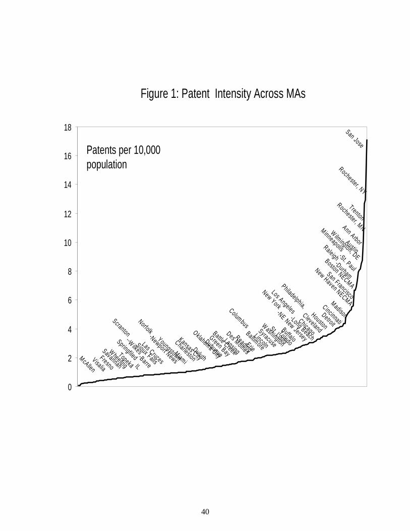
40

Figure 1: Patent Intensity Across MAs

Log of Patents per 10,000 population

McAllenVisalia

Fresno

Savannah

WheelingTopeka

Springfiled, IL

Scranton--W ilkes-Barre

Sioux Falls

Las Cruces

Norfolk-Newport News

YoungstownMiami

Charleston

Kansas CityDuluth

Oklahoma City

Dubuque

Green Bay

Battle Creek

Lansing

Des Moines

ReadingErie

ColumbusBaltimore

Lincoln

Syracuse

Washington

St. LouisToledo

Buffalo

New York-NE New Jersey

Los Angeles-Long Beach

Philadelphia,

Chicago

Cleveland

Houston

Detroit

Cincinnati

Madison

New Haven NECMA

San Francisco

Boston NECMA

Raleigh-Durham

Minneapolis-St. Paul

W ilmington, DE

Austin

Ann Arbor

Rochester, MN

Trenton

Rochester, NY

San Jose

0

2

4

6

8

10

12

14

16

18

Patents per 10,000 population

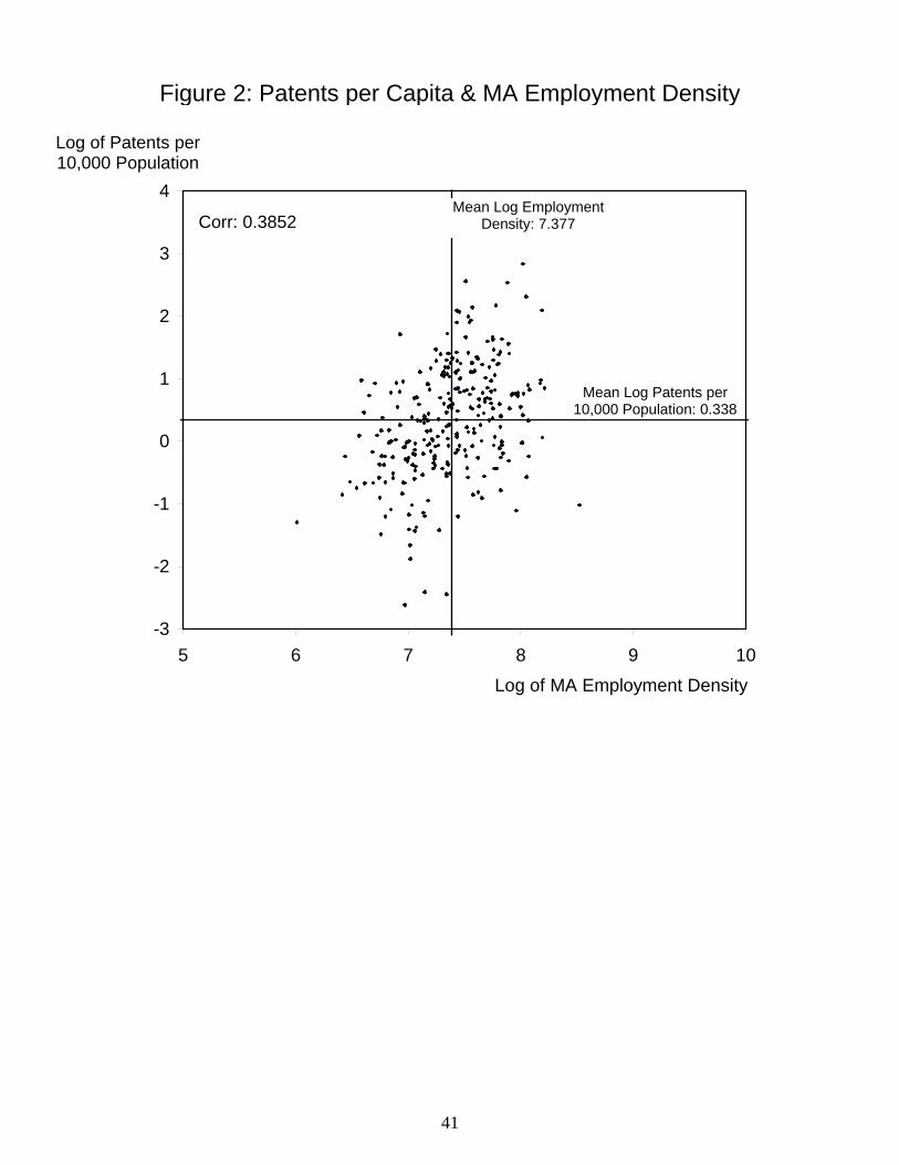
41

-3

-2

-1

0

1

2

3

4

5 6 7 8 9 10

Log of MA Employment Density

Figure 2: Patents per Capita & MA Employment Density

Log of Patents per 10,000 Population

Mean Log EmploymentDensity: 7.377

Mean Log Patents per 10,000 Population: 0.338

Corr: 0.3852

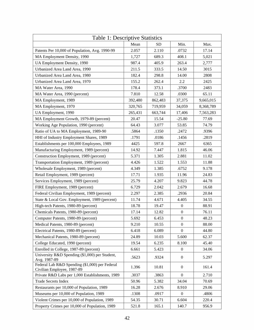
42

Table 1: Descriptive Statistics Mean SD Min. Max.

Patents Per 10,000 of Population, Avg. 1990-99 2.057 2.110 .0732 17.14 MA Employment Density, 1990 1,727 689.3 408.1 5,021 UA Employment Density, 1990 987.4 405.9 263.4 2,777 Urbanized Area Land Area, 1990 211.5 333.5 14.50 3015 Urbanized Area Land Area, 1980 182.4 298.8 14.00 2808 Urbanized Area Land Area, 1970 155.2 262.4 2.2 2425 MA Water Area, 1990 178.4 373.1 .3700 2483 MA Water Area, 1990 (percent) 7.810 12.58 .0300 65.11 MA Employment, 1989 392,480 862,483 37,375 9,665,015 MA Employment, 1970 320,765 719,959 34,059 8,368,789 UA Employment, 1990 265,431 663,744 17,406 7,563,283 MA Employment Growth, 1979-89 (percent) 20.47 15.54 -25.80 77.69 Working Age Population, 1990 (percent) 64.43 3.077 53.85 74.79 Ratio of UA to MA Employment, 1989-90 .5864 .1350 .2472 .9396 HHI of Industry Employment Shares, 1989 .1791 .0186 .1456 .2819 Establishments per 100,000 Employees, 1989 4425 597.8 2667 6365 Manufacturing Employment, 1989 (percent) 14.92 7.447 1.815 46.06 Construction Employment, 1989 (percent) 5.371 1.305 2.881 11.02 Transportation Employment, 1989 (percent) 4.426 1.522 1.553 11.88 Wholesale Employment, 1989 (percent) 4.349 1.385 .6752 9.178 Retail Employment, 1989 (percent) 17.71 1.935 11.96 24.83 Services Employment, 1989 (percent) 25.79 4.207 9.823 44.78 FIRE Employment, 1989 (percent) 6.729 2.042 2.679 16.68 Federal Civilian Employment, 1989 (percent) 2.297 2.385 .2936 20.84 State & Local Gov. Employment, 1989 (percent) 11.74 4.671 4.405 34.55 High-tech Patents, 1980-89 (percent) 18.78 19.47 0 88.91 Chemicals Patents, 1980-89 (percent) 17.14 12.82 0 76.11 Computer Patents, 1980-89 (percent) 5.692 6.453 0 48.23 Medical Patents, 1980-89 (percent) 9.210 10.55 0 88.00 Electrical Patents, 1980-89 (percent) 6.418 6.089 0 44.80 Mechanical Patents, 1980-89 (percent) 24.89 10.03 5.600 62.37 College Educated, 1990 (percent) 19.54 6.235 8.100 45.40 Enrolled in College, 1987-89 (percent) 6.661 5.423 0 34.06 University R&D Spending ($1,000) per Student, Avg. 1987-89 .5623 .9324 0 5.297

Federal Lab R&D Spending ($1,000) per Federal Civilian Employee, 1987-89 1.396 10.81 0 161.4

Private R&D Labs per 1,000 Establishments, 1989 .3037 .3863 0 2.710 Trade Secrets Index 50.96 5.382 34.04 70.69 Restaurants per 10,000 of Population, 1989 16.28 2.676 8.910 29.06 Museums per 10,000 of Population, 1989 .1308 .0917 0 .4806 Violent Crimes per 10,000 of Population, 1989 54.35 30.71 6.604 220.4 Property Crimes per 10,000 of Population, 1989 521.8 165.1 140.7 956.9

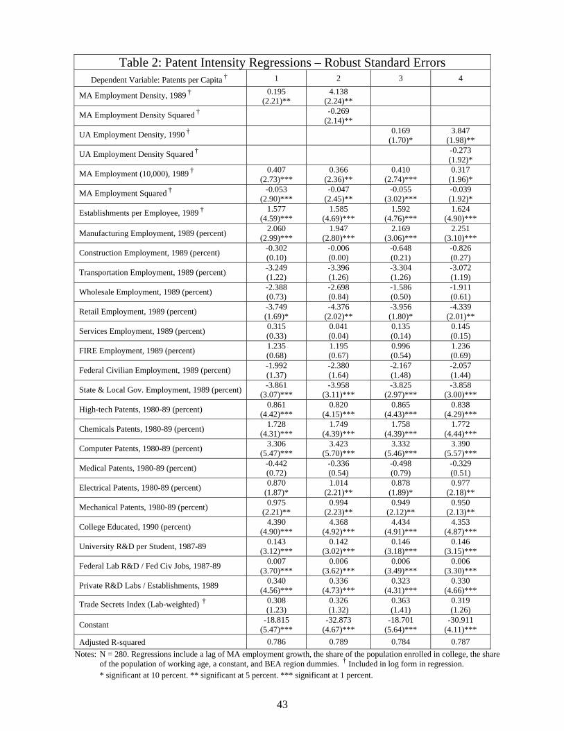
43

Table 2: Patent Intensity Regressions – Robust Standard Errors Dependent Variable: Patents per Capita † 1 2 3 4

MA Employment Density, 1989 † 0.195 (2.21)**

4.138 (2.24)**

MA Employment Density Squared † -0.269 (2.14)**

UA Employment Density, 1990 † 0.169 (1.70)*

3.847 (1.98)**

UA Employment Density Squared † -0.273 (1.92)*

MA Employment (10,000), 1989 † 0.407 (2.73)***

0.366 (2.36)**

0.410 (2.74)***

0.317 (1.96)*

MA Employment Squared † -0.053 (2.90)***

-0.047 (2.45)**

-0.055 (3.02)***

-0.039 (1.92)*

Establishments per Employee, 1989 † 1.577 (4.59)***

1.585 (4.69)***

1.592 (4.76)***

1.624 (4.90)***

Manufacturing Employment, 1989 (percent) 2.060 (2.99)***

1.947 (2.80)***

2.169 (3.06)***

2.251 (3.10)***

Construction Employment, 1989 (percent) -0.302 (0.10)

-0.006 (0.00)

-0.648 (0.21)

-0.826 (0.27)

Transportation Employment, 1989 (percent) -3.249 (1.22)

-3.396 (1.26)

-3.304 (1.26)

-3.072 (1.19)

Wholesale Employment, 1989 (percent) -2.388 (0.73)

-2.698 (0.84)

-1.586 (0.50)

-1.911 (0.61)

Retail Employment, 1989 (percent) -3.749 (1.69)*

-4.376 (2.02)**

-3.956 (1.80)*

-4.339 (2.01)**

Services Employment, 1989 (percent) 0.315 (0.33)

0.041 (0.04)

0.135 (0.14)

0.145 (0.15)

FIRE Employment, 1989 (percent) 1.235 (0.68)

1.195 (0.67)

0.996 (0.54)

1.236 (0.69)

Federal Civilian Employment, 1989 (percent) -1.992 (1.37)

-2.380 (1.64)

-2.167 (1.48)

-2.057 (1.44)

State & Local Gov. Employment, 1989 (percent) -3.861 (3.07)***

-3.958 (3.11)***

-3.825 (2.97)***

-3.858 (3.00)***

High-tech Patents, 1980-89 (percent) 0.861 (4.42)***

0.820 (4.15)***

0.865 (4.43)***

0.838 (4.29)***

Chemicals Patents, 1980-89 (percent) 1.728 (4.31)***

1.749 (4.39)***

1.758 (4.39)***

1.772 (4.44)***

Computer Patents, 1980-89 (percent) 3.306 (5.47)***

3.423 (5.70)***

3.332 (5.46)***

3.390 (5.57)***

Medical Patents, 1980-89 (percent) -0.442 (0.72)

-0.336 (0.54)

-0.498 (0.79)

-0.329 (0.51)

Electrical Patents, 1980-89 (percent) 0.870 (1.87)*

1.014 (2.21)**

0.878 (1.89)*

0.977 (2.18)**

Mechanical Patents, 1980-89 (percent) 0.975 (2.21)**

0.994 (2.23)**

0.949 (2.12)**

0.950 (2.13)**

College Educated, 1990 (percent) 4.390 (4.90)***

4.368 (4.92)***

4.434 (4.91)***

4.353 (4.87)***

University R&D per Student, 1987-89 0.143 (3.12)***

0.142 (3.02)***

0.146 (3.18)***

0.146 (3.15)***

Federal Lab R&D / Fed Civ Jobs, 1987-89 0.007 (3.70)***

0.006 (3.62)***

0.006 (3.49)***

0.006 (3.30)***

Private R&D Labs / Establishments, 1989 0.340 (4.56)***

0.336 (4.73)***

0.323 (4.31)***

0.330 (4.66)***

Trade Secrets Index (Lab-weighted) † 0.308 (1.23)

0.326 (1.32)

0.363 (1.41)

0.319 (1.26)

Constant -18.815 (5.47)***

-32.873 (4.67)***

-18.701 (5.64)***

-30.911 (4.11)***

Adjusted R-squared 0.786 0.789 0.784 0.787 Notes: N = 280. Regressions include a lag of MA employment growth, the share of the population enrolled in college, the share

of the population of working age, a constant, and BEA region dummies. † Included in log form in regression. * significant at 10 percent. ** significant at 5 percent. *** significant at 1 percent.

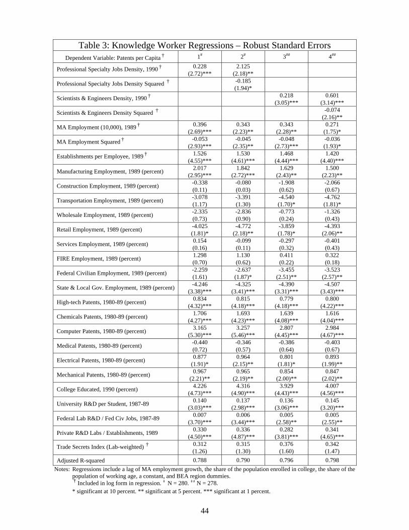
44

Table 3: Knowledge Worker Regressions – Robust Standard Errors Dependent Variable: Patents per Capita † 1# 2# 3## 4##

0.228 2.125 Professional Specialty Jobs Density, 1990 † (2.72)*** (2.18)**

-0.185 Professional Specialty Jobs Density Squared † (1.94)* 0.218 0.601 Scientists & Engineers Density, 1990 † (3.05)*** (3.14)*** -0.074 Scientists & Engineers Density Squared † (2.16)**

0.396 0.343 0.343 0.271 MA Employment (10,000), 1989 † (2.69)*** (2.23)** (2.28)** (1.75)*

-0.053 -0.045 -0.048 -0.036 MA Employment Squared † (2.93)*** (2.35)** (2.73)*** (1.93)*

1.526 1.530 1.468 1.420 Establishments per Employee, 1989 † (4.55)*** (4.61)*** (4.44)*** (4.40)***

2.017 1.842 1.629 1.500 Manufacturing Employment, 1989 (percent) (2.95)*** (2.72)*** (2.43)** (2.23)** -0.338 -0.080 -1.908 -2.066 Construction Employment, 1989 (percent) (0.11) (0.03) (0.62) (0.67) -3.078 -3.391 -4.540 -4.762 Transportation Employment, 1989 (percent) (1.17) (1.30) (1.70)* (1.81)* -2.335 -2.836 -0.773 -1.326 Wholesale Employment, 1989 (percent) (0.73) (0.90) (0.24) (0.43) -4.025 -4.772 -3.859 -4.393 Retail Employment, 1989 (percent) (1.81)* (2.18)** (1.78)* (2.06)** 0.154 -0.099 -0.297 -0.401 Services Employment, 1989 (percent) (0.16) (0.11) (0.32) (0.43) 1.298 1.130 0.411 0.322 FIRE Employment, 1989 (percent) (0.70) (0.62) (0.22) (0.18) -2.259 -2.637 -3.455 -3.523 Federal Civilian Employment, 1989 (percent) (1.61) (1.87)* (2.51)** (2.57)** -4.246 -4.325 -4.390 -4.507 State & Local Gov. Employment, 1989 (percent) (3.38)*** (3.41)*** (3.31)*** (3.43)*** 0.834 0.815 0.779 0.800 High-tech Patents, 1980-89 (percent) (4.32)*** (4.18)*** (4.18)*** (4.22)*** 1.706 1.693 1.639 1.616 Chemicals Patents, 1980-89 (percent) (4.27)*** (4.23)*** (4.08)*** (4.04)*** 3.165 3.257 2.807 2.984 Computer Patents, 1980-89 (percent) (5.30)*** (5.46)*** (4.45)*** (4.67)*** -0.440 -0.346 -0.386 -0.403 Medical Patents, 1980-89 (percent) (0.72) (0.57) (0.64) (0.67) 0.877 0.964 0.801 0.893 Electrical Patents, 1980-89 (percent) (1.91)* (2.15)** (1.81)* (1.99)** 0.967 0.965 0.854 0.847 Mechanical Patents, 1980-89 (percent) (2.21)** (2.19)** (2.00)** (2.02)** 4.226 4.316 3.929 4.007 College Educated, 1990 (percent) (4.73)*** (4.90)*** (4.43)*** (4.56)*** 0.140 0.137 0.136 0.145 University R&D per Student, 1987-89 (3.03)*** (2.98)*** (3.06)*** (3.20)*** 0.007 0.006 0.005 0.005 Federal Lab R&D / Fed Civ Jobs, 1987-89 (3.70)*** (3.44)*** (2.58)** (2.55)** 0.330 0.336 0.282 0.341 Private R&D Labs / Establishments, 1989 (4.50)*** (4.87)*** (3.81)*** (4.65)*** 0.312 0.315 0.376 0.342 Trade Secrets Index (Lab-weighted) † (1.26) (1.30) (1.60) (1.47)

Adjusted R-squared 0.788 0.790 0.796 0.798 Notes: Regressions include a lag of MA employment growth, the share of the population enrolled in college, the share of the

population of working age, a constant, and BEA region dummies. † Included in log form in regression. # N = 280. ## N = 278.

* significant at 10 percent. ** significant at 5 percent. *** significant at 1 percent.

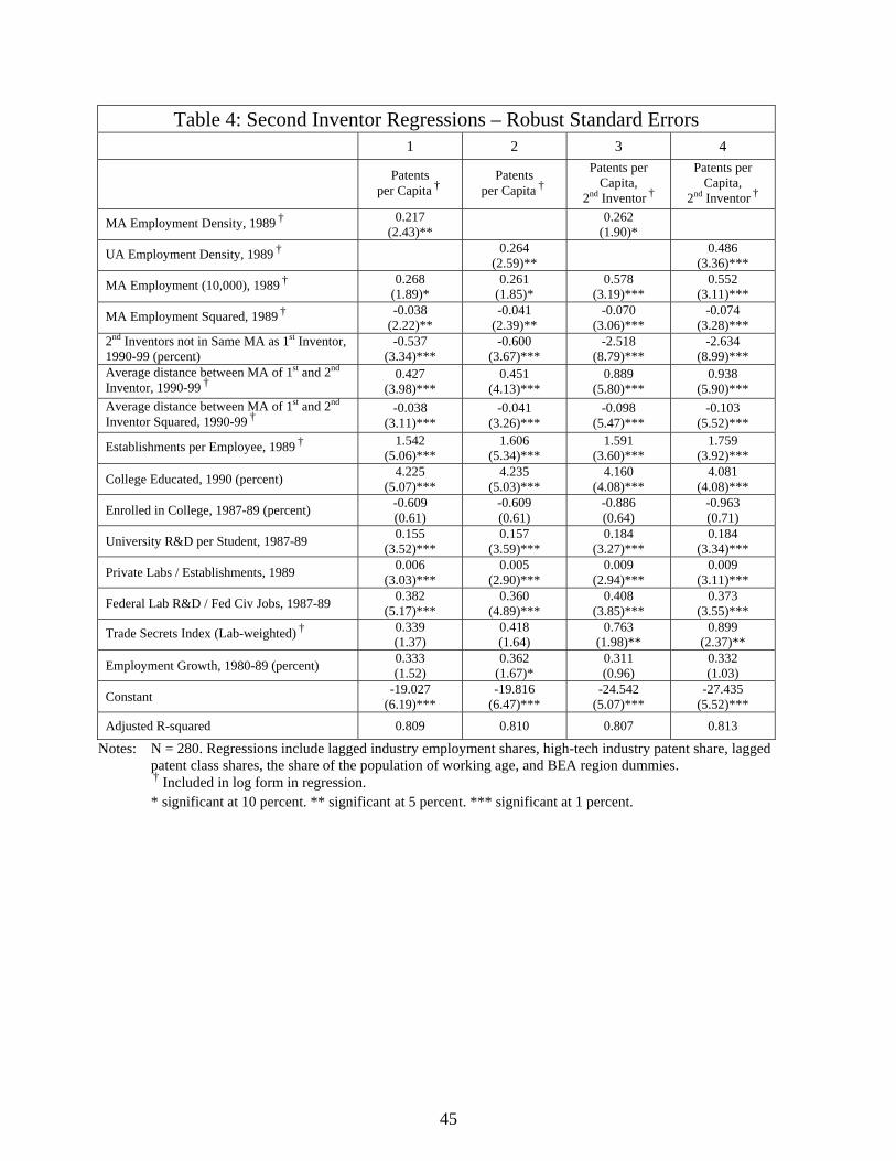
45

Table 4: Second Inventor Regressions – Robust Standard Errors 1 2 3 4

Patents

per Capita † Patents

per Capita †

Patents per Capita,

2nd Inventor †

Patents per Capita,

2nd Inventor †

MA Employment Density, 1989 † 0.217 (2.43)** 0.262

(1.90)*

UA Employment Density, 1989 † 0.264 (2.59)** 0.486

(3.36)***

MA Employment (10,000), 1989 † 0.268 (1.89)*

0.261 (1.85)*

0.578 (3.19)***

0.552 (3.11)***

MA Employment Squared, 1989 † -0.038 (2.22)**

-0.041 (2.39)**

-0.070 (3.06)***

-0.074 (3.28)***

2nd Inventors not in Same MA as 1st Inventor, 1990-99 (percent)

-0.537 (3.34)***

-0.600 (3.67)***

-2.518 (8.79)***

-2.634 (8.99)***

Average distance between MA of 1st and 2nd Inventor, 1990-99 †

0.427 (3.98)***

0.451 (4.13)***

0.889 (5.80)***

0.938 (5.90)***

Average distance between MA of 1st and 2nd Inventor Squared, 1990-99 †

-0.038 (3.11)***

-0.041 (3.26)***

-0.098 (5.47)***

-0.103 (5.52)***

Establishments per Employee, 1989 † 1.542 (5.06)***

1.606 (5.34)***

1.591 (3.60)***

1.759 (3.92)***

College Educated, 1990 (percent) 4.225 (5.07)***

4.235 (5.03)***

4.160 (4.08)***

4.081 (4.08)***

Enrolled in College, 1987-89 (percent) -0.609 (0.61)

-0.609 (0.61)

-0.886 (0.64)

-0.963 (0.71)

University R&D per Student, 1987-89 0.155 (3.52)***

0.157 (3.59)***

0.184 (3.27)***

0.184 (3.34)***

Private Labs / Establishments, 1989 0.006 (3.03)***

0.005 (2.90)***

0.009 (2.94)***

0.009 (3.11)***

Federal Lab R&D / Fed Civ Jobs, 1987-89 0.382 (5.17)***

0.360 (4.89)***

0.408 (3.85)***

0.373 (3.55)***

Trade Secrets Index (Lab-weighted) † 0.339 (1.37)

0.418 (1.64)

0.763 (1.98)**

0.899 (2.37)**

Employment Growth, 1980-89 (percent) 0.333 (1.52)

0.362 (1.67)*

0.311 (0.96)

0.332 (1.03)

Constant -19.027 (6.19)***

-19.816 (6.47)***

-24.542 (5.07)***

-27.435 (5.52)***

Adjusted R-squared 0.809 0.810 0.807 0.813

Notes: N = 280. Regressions include lagged industry employment shares, high-tech industry patent share, lagged patent class shares, the share of the population of working age, and BEA region dummies.

† Included in log form in regression. * significant at 10 percent. ** significant at 5 percent. *** significant at 1 percent.

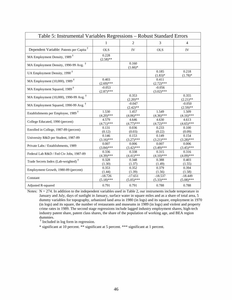
46

Table 5: Instrumental Variables Regressions – Robust Standard Errors 1 2 3 4

Dependent Variable: Patents per Capita † OLS IV OLS IV

MA Employment Density, 1989 † 0.228 (2.58)**

MA Employment Density, 1990-99 Avg. † 0.160 (1.66)*

UA Employment Density, 1990 † 0.185 (1.83)*

0.218 (1.78)*

MA Employment (10,000), 1989 † 0.403 (2.69)*** 0.411

(2.72)***

MA Employment Squared, 1989 † -0.053 (2.87)*** -0.056

(3.02)***

MA Employment (10,000), 1990-99 Avg. † 0.353 (2.20)** 0.355

(2.21)**

MA Employment Squared, 1990-99 Avg. † -0.047 (2.42)** -0.050

(2.59)**

Establishments per Employee, 1989 † 1.530 (4.20)***

1.457 (4.06)***

1.549 (4.36)***

1.509 (4.16)***

College Educated, 1990 (percent) 4.579 (4.71)***

4.646 (4.77)***

4.630 (4.72)***

4.613 (4.65)***

Enrolled in College, 1987-89 (percent) 0.131 (0.12)

0.036 (0.03)

0.233 (0.22)

0.100 (0.09)

University R&D per Student, 1987-89 0.146 (3.16)***

0.153 (3.27)***

0.149 (3.21)***

0.154 (3.28)***

Private Labs / Establishments, 1989 0.007 (3.84)***

0.006 (3.42)***

0.007 (3.49)***

0.006 (3.45)***

Federal Lab R&D / Fed Civ Jobs, 1987-89 0.336 (4.39)***

0.338 (4.41)***

0.315 (4.10)***

0.316 (4.09)***

Trade Secrets Index (Lab-weighted) † 0.328 (1.30)

0.348 (1.37)

0.388 (1.49)

0.403 (1.55)

Employment Growth, 1980-89 (percent) 0.353 (1.44)

0.352 (1.39)

0.379 (1.56)

0.394 (1.58)

Constant -18.726 (5.18)***

-17.651 (5.05)***

-18.537 (5.33)***

-18.449 (5.08)***

Adjusted R-squared 0.791 0.791 0.788 0.788

Notes: N = 274. In addition to the independent variables used in Table 2, our instruments include temperature in January and July, days of sunlight in January, surface water in square miles and as a share of total area, 5 dummy variables for topography, urbanized land area in 1980 (in logs) and its square, employment in 1970 (in logs) and its square, the number of restaurants and museums in 1989 (in logs) and violent and property crime rates in 1989. The second stage regressions include lagged industry employment shares, high-tech industry patent share, patent class shares, the share of the population of working age, and BEA region dummies.

† Included in log form in regression. * significant at 10 percent. ** significant at 5 percent. *** significant at 1 percent.

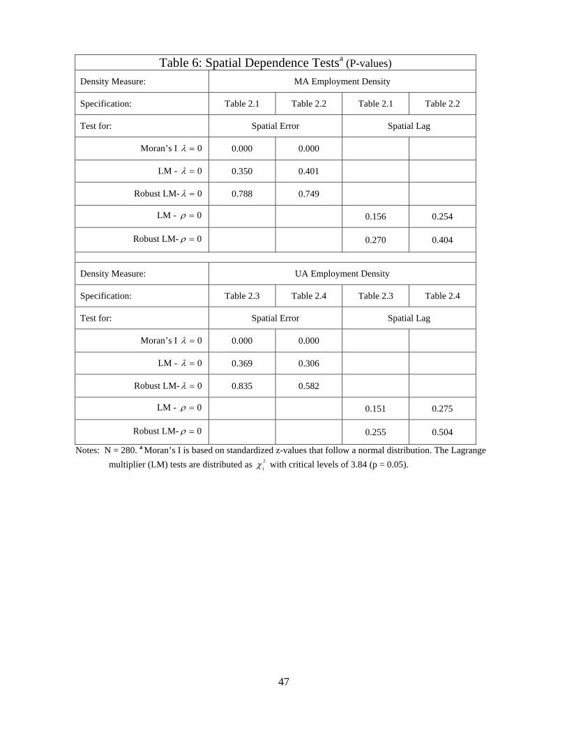
47

Table 6: Spatial Dependence Testsa (P-values) Density Measure: MA Employment Density

Specification: Table 2.1 Table 2.2 Table 2.1 Table 2.2

Test for: Spatial Error Spatial Lag

Moran’s I 0λ = 0.000 0.000

LM - 0λ = 0.350 0.401

Robust LM- 0λ = 0.788 0.749

LM - 0ρ = 0.156 0.254

Robust LM- 0ρ = 0.270 0.404

Density Measure: UA Employment Density

Specification: Table 2.3 Table 2.4 Table 2.3 Table 2.4

Test for: Spatial Error Spatial Lag

Moran’s I 0λ = 0.000 0.000

LM - 0λ = 0.369 0.306

Robust LM- 0λ = 0.835 0.582

LM - 0ρ = 0.151 0.275

Robust LM- 0ρ = 0.255 0.504

Notes: N = 280. a Moran’s I is based on standardized z-values that follow a normal distribution. The Lagrange multiplier (LM) tests are distributed as 2

1χ with critical levels of 3.84 (p = 0.05).

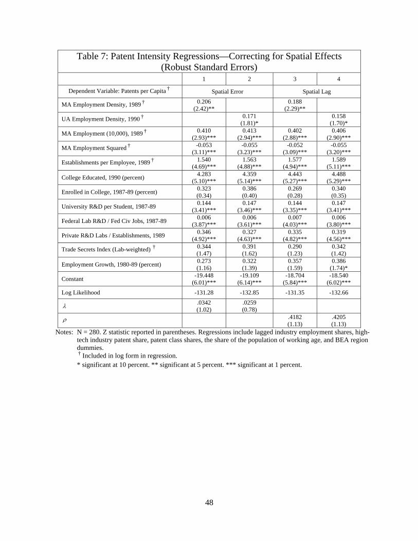
48

Table 7: Patent Intensity Regressions—Correcting for Spatial Effects

(Robust Standard Errors) 1 2 3 4

Dependent Variable: Patents per Capita † Spatial Error Spatial Lag

MA Employment Density, 1989 † 0.206 (2.42)** 0.188

(2.29)**

UA Employment Density, 1990 † 0.171 (1.81)* 0.158

(1.70)*

MA Employment (10,000), 1989 † 0.410 (2.93)***

0.413 (2.94)***

0.402 (2.88)***

0.406 (2.90)***

MA Employment Squared † -0.053 (3.11)***

-0.055 (3.23)***

-0.052 (3.09)***

-0.055 (3.20)***

Establishments per Employee, 1989 † 1.540 (4.69)***

1.563 (4.88)***

1.577 (4.94)***

1.589 (5.11)***

College Educated, 1990 (percent) 4.283 (5.10)***

4.359 (5.14)***

4.443 (5.27)***

4.488 (5.29)***

Enrolled in College, 1987-89 (percent) 0.323 (0.34)

0.386 (0.40)

0.269 (0.28)

0.340 (0.35)

University R&D per Student, 1987-89 0.144 (3.41)***

0.147 (3.46)***

0.144 (3.35)***

0.147 (3.41)***

Federal Lab R&D / Fed Civ Jobs, 1987-89 0.006 (3.87)***

0.006 (3.61)***

0.007 (4.03)***

0.006 (3.80)***

Private R&D Labs / Establishments, 1989 0.346 (4.92)***

0.327 (4.63)***

0.335 (4.82)***

0.319 (4.56)***

Trade Secrets Index (Lab-weighted) † 0.344 (1.47)

0.391 (1.62)

0.290 (1.23)

0.342 (1.42)

Employment Growth, 1980-89 (percent) 0.273 (1.16)

0.322 (1.39)

0.357 (1.59)

0.386 (1.74)*

Constant -19.448 (6.01)***

-19.109 (6.14)***

-18.704 (5.84)***

-18.540 (6.02)***

Log Likelihood -131.28 -132.85 -131.35 -132.66

λ .0342 (1.02)

.0259 (0.78)

ρ .4182 (1.13)

.4205 (1.13)

Notes: N = 280. Z statistic reported in parentheses. Regressions include lagged industry employment shares, high-tech industry patent share, patent class shares, the share of the population of working age, and BEA region dummies.

† Included in log form in regression. * significant at 10 percent. ** significant at 5 percent. *** significant at 1 percent.