Urban Density and Pupil Attainment

Stephen Gibbons

Olmo Silva

May 2007

Published by

Centre for the Economics of Education

London School of Economics

Houghton Street

London WC2A 2AE

© Stephen Gibbons and Olmo Silva, submitted November 2006

May 2007

ISBN 978-0-85328-202-0

The Centre for the Economics of Education is an independent research centre funded by the Department for Children, Schools & Families. The views expressed in this work are those of the author and do not reflect the views of the DCSF. All errors and omissions remain the authors.

Executive Summary

Among policy markers, school inspectors and parents, there is a widespread belief that inner-

city schools fail to provide their pupils with an environment that is conducive to high

standards of education. Yet, to researchers interested in urbanization and agglomeration

economics this sounds surprising: schools in denser environments can potentially benefit

from a deeper pool of good teachers in urban labour markets, better inter-school networking

and common infrastructures. Further, pupils in more urban environments have a wider set of

schools from which they can choose. So, if students with many available schools can be more

efficiently matched to educational providers that suit their preferences and capabilities then

average educational standards should increase. Finally, proximity of urban schools might

provide incentives for improvement and adoption of new teaching technologies through

competition, or cooperation, with other educational provides. Why then do so many observers

come to the conclusion that inner-city schools are irremediably ‘failing schools’?

In this study, we argue that this remark is based on the simple, but fallacious,

observation that a large proportion of low achievers are concentrated in dense urban places.

Although attainment in dense urban places is low on average, this is not because urban

environments disadvantage pupils, but because the most disadvantaged pupils with low

average attainments attend the most urbanised schools. As widely recognised, cities have a

high concentration of children with fewer home resources and other family background

disadvantages and who on average do worse at school. While this suggests that urban schools

are building ‘human capital’ on a lower base in terms of pupil characteristics, it does not

necessarily have any bearing on the educational progress of children in city areas or on the

effectiveness of urban schools in educating their pupils.

In our paper we use a census of over 1.2 million pupils in England, matched to records

on their academic progress, to assess whether pupils in city schools really show low-

educational progress relative to schools in lower density suburban, semi-rural and rural areas.

To answer this question, we compare the improvement or decline in the attainment of pupils

who shared the same Primary school but move from low-density to high-density areas or

vice-versa on compulsory transition to Secondary school. Our strategy allows us to control

for individual unobservable characteristics that are fixed over time (such as family

background, innate abilities or young-age experiences and peer influences), which may

negatively affect the academic performance of students in schools in inner cities.

We find evidence of small but significant benefits from education in schools in more densely

urbanised settings. In particular, we show that:

• Pupils in schools in relatively dense places – that is in areas with a higher density

of schools, more continuous urban land cover and higher population density –

progress faster than others in their cohort. This urban density effect is, however,

fairly small in magnitude – a 10% relative increase in urban density raises a

pupils ranking in terms of academic qualifications by about 0.2% between ages

12 and 16.

• Amongst the three density measures we study, the number of neighbouring

schools always dominates in terms of its importance in raising a pupil’s ranking

in the distribution of academic achievement.

• The density advantage is detectable even amongst pupils moving relatively short

distances between Primary and Secondary schools within Local Authorities and

within urban areas. This suggests that our results cannot be explained solely by

broad urbanisation effects experienced by pupils making rural-urban school

moves.

• Finally, progress during Secondary school is only related to the density of local

Secondary schools, and not linked to the number of local Primary schools. We

argue this provides evidence on the effects of greater school choice and inter-

school competition between closely co-located institutions in more urban

settings.

Although the elasticity of pupil attainment with respect to school density that we detect is

small, simple calculations show that moving from the least to the most urbanized

environment would result in a 2.5-2.8 percentile increase in the attainment distribution at age

16, relative to age 11. This is comparable to the gap between poor pupils who are entitled free

school meals and others, and only slightly less than the gender gap (4 percentiles), which has

been the subject of much academic attention. Even so, these gains are not large enough to

close the gap in the level of attainments of pupils in the most urban schools relative to

students in more rural areas at the end of Secondary compulsory education, which remain as

large as 8.5 percentiles.

Urban Density and Pupil Attainment

Stephen Gibbons

Olmo Silva

1. Introduction 1

2. The Literature 2

3. Empirical Methods: The Value Added Model of Attainment 6

4. The Data 10

Schools, pupils and tests

Indices of urban density 12

5. Results and Discussion 13

Descriptive statistics 13

Estimates of the attainment models 15

Estimates of one and two-way fixed effects models 18

Geographical scope: who benefits? 20

Robustness checks: strategic behaviour, mean reversion, pre-transition

trends, greater urban heterogeneity? 22

Looking for an explanation: school choice and competition,

resources or policy 28

6. Conclusions 30

References 32

Figures 36

Tables 37

Appendices 43

Acknowledgments

The authors would like to thank Joan Wilson, Helena Holmlund, Stephen Machin and

participants at the International Conference on “Empirical Methods for the Study of

Economic Agglomerations”, Kyoto, June 2006 and at the 3rd EEEPE-CEPR Conference,

Paris, October 2006.

Stephen Gibbons is a lecturer in Economic Geography at the Department of Geography and

Environment, London School of Economics (LSE), and a Research Associate at the Centre for

Economic Performance, LSE and the Centre for the Economics of Education. Olmo Silva is a

Research Officer at the Centre for the Economics of Education and at the Centre for

Economic Performance, London School of Economics.

1. Introduction

City schools in the US, UK and elsewhere are widely admonished by politicians, schools

inspectors, parents and academics for failing to provide pupils with high standards of

education (see discussions in Machin and Vignoles, 2005, Murnane, 2002, Neal, 1997 and

Ofsted, 2003). With the aim of redressing this situation, governments in many countries have

increasingly targeted schools in disadvantaged urban areas; among others, recent policy

interventions include the ‘Excellence in Cities’ program discussed in Machin et al. (2006),

the ‘Aimhigher’ initiative described in Emmerson et al. (2006), and the STAR experiment

debated in Hanushek (2003) and Krueger (2003).

In some ways, this should come as something as a surprise to economists interested in the

benefits of urbanisation and agglomeration: City schools can potentially draw from a diverse

pool of high-quality teachers and are geographically placed in settings which should provide

incentives through competition with other schools, and facilitate sharing of teaching know-

how and technology through cooperation. Of course, given the concentration of poverty in

cities, it is also recognised that urban schools are building human capital on a lower base in

terms of pupil characteristics, in particular higher rates of hardship and lower initial ability.

However, this rarely seems to be taken into account when drawing inferences about the

effectiveness of urban schools; the simple observation of a high concentration of low

achievers in dense urban places is taken as evidence that urban environments disadvantage

pupils.

This paper uses a census of over 1.2 million pupils in England, matched to records on their

academic progress, to assess whether pupils in city schools really show low-educational

progress relative to schools in lower density suburban, semi-rural and rural areas. We use

information on the improvement or decline in the attainment of pupils who shared the same

Primary school, but then move from low-density to high-density areas or vice-versa on

compulsory transition to Secondary school. We find evidence of small but significant benefits

from education in schools in more densely urbanised settings: Pupils in schools in relatively

dense places – measured in terms of school density and other urban indicators – progress

faster than others in their cohort, although the elasticity is low, at around 0.02. We find this

1

association even amongst pupils moving relatively short distances between Primary and

Secondary schools within urban areas; so, we argue, our results do not emerge from broad

agglomeration and urbanisation effects experienced by pupils making rural-urban school

moves. Instead, we interpret our findings as providing evidence on the effects of greater

school choice and inter-school competition between closely co-located institutions in more

urban settings.

The paper has the following structure. The next section outlines some relevant literature and

sets the work in the context of studies on agglomeration and urbanization economies. Section

3 sets out our empirical approach, while section 4 describes the data. Section 5 presents and

discusses the results that arise from these approaches, and we make some concluding remarks

in section 6.

2. The Literature

“Conceptually, a city is just a dense agglomeration of people and firms. All of the benefits of

cities ultimately come from reduced transport costs for goods, people and ideas” (Glaeser,

1998). This simple intuition, borrowed from the seminal writings of Marshall (1920), is

nowadays at the core of most research on agglomeration and urbanisation processes. In a

nutshell, the fundamental reason why firms and workers concentrate in geographically

contained areas, giving rise to cities, is because clustering generates some forms of

economies of scale, or increasing returns, due to proximity. As discussed in Glaeser (1998)

and Rosenthal and Strange (2001), these mainly emerge from proximity in three factors:

People, associated with labour market pooling and accessibility to a wider sets of customers;

Goods, coupled with input sharing and specialization of services for producers; Ideas, linked

to the emergence of knowledge and technological spillovers across firms. While proximity of

goods and individuals seems a natural requirement for of economies of scale to emerge in

urban environments, it could be argued that knowledge spillovers are not constrained by

distance, or within the boundaries of urban areas. Yet, Jaffe et al. (1993) provides strong

evidence on the importance of proximity for know-how diffusion too. So, along all these

three dimensions, closeness seems to be the channel through which urban areas generate

2

productivity benefits for both workers and firms.

Technological spillovers are also often invoked as an explanation for the reason why cities

not only exist, but prosper and grow too: Knowledge spillovers between neighbouring firms

within an industry generate dynamic agglomeration economies, leading to faster pace of

innovation, continuous improvements in modes of production, and affecting growth rates of

productivity, output and employment. While in the original Marshallian (1890) setting

dynamic economies emerge because the concentration of an industry in a city gives rise to

local monopolies that internalize the benefits of innovation and encourage it, Porter (1990)

argues that it is the more intense competition among close firms in a specialized location that

gives rise to dynamic agglomeration economies. Whatever one’s view here, most academics

now agree on the relevance of geographical proximity for knowledge flows to take place and

dynamic agglomeration economies to emerge.

For these reasons, the idea that urban schools fail to provide pupils with a high standard

environment for learning comes as something as a surprise to researchers interested in

economies of urbanization and agglomeration: City schools have the potential to exploit

dense labour markets, therefore attracting high-quality teachers; city schools are located in

diversified areas where pupils and teachers can be more efficiently matched through the

exercise of school choice; city schools face a large and heterogeneous pool of ‘consumers’,

thus having potential to exploit economies from specialization; pupils in urban schools may

also benefit from learning spillovers associated with closer connections to a larger and more

diverse group of students. Further, city schools share better common infrastructures, e.g.

faster connection for use of information technologies or public transport; finally, city schools

are geographically placed in settings which should provide incentives for improvement or

adoption of new teaching technologies through competition with other schools, and facilitate

sharing of teaching know-how through cooperation. What evidence is available?

A growing body of research on the functioning of the labour market for teachers has been

produced over the past years. Using different methodologies and data, Dolton and van der

Klaauw (1995), Hanushek et al. (2003a and 2003b), Murnane and Olson (1989 and 1990) all

show that individuals mainly respond to (relative) wage incentives in their decision to start

teaching or leave this occupation. Chevalier et al. (2002) confirm this finding for a longer

3

time horizon (1960s to 1990s), and show that graduates have a lower probability of becoming

teachers in urban areas; this might be because teaching is a poor option compared to more

remunerative alternatives available in these locations, or because working conditions in urban

schools are perceived to be worse than in provincial areas or other occupations. This is

consistent with evidence in Hanushek et al. (2003b), showing that teachers changing schools

within urban districts seek out schools with easier to teach pupils, such as private schools.

However, whether this results in lower teacher quality in urban schools is open to debate.

Hanushek et al. (2005) suggests the opposite is true: Teachers exiting Texas public urban

schools are on average less effective at raising pupil attainments than those who stay;

moreover, there is no evidence to support the idea that urban schools loose their best teachers

to suburban and rural schools. Additionally, Hanushek et al. (2003a) and Lavy (2005) show

that teacher performance-related pay has great potential for retaining effective teachers in city

schools, improving their motivation and increasing pupils’ attainments. Finally, Clotfelter et

al. (2006) show that a pecuniary bonus granted to qualified teachers in North Carolina greatly

reduced their hazard of leaving high-poverty schools; this was especially pronounced for

teachers with longer years of experience, associated to better pupil outcomes (see Hanushek

et al., 2005). Overall then, city schools seem to be in a favourable position to exploit labour

markets to hire and retain high-quality educators.

The benefits of choice and competition among schools should also have greater scope in

urban areas. A large number of closely located schools imply that parents have a wider set of

schools to choose from within feasible travel-distance; if pupils with many available schools

can be more efficiently matched to educational providers that suit their preferences and

capabilities, average educational standards should increase. Moreover, in a school market

where parents can exercise choice and funding follows pupils (as in the UK setting)1, schools

have to provide ‘quality’ that parents demand or face falling enrolment, loss of money and

ultimately closure. Proximity of urban schools therefore seems to provide incentives for

improvement and adoption of new teaching technologies through competition with other

1 And there is no strict zoning, i.e. pupils can attend every non-oversubscribed school of their choice, without

restrictions regarding place of residence and school proximity.

4

educational provides. In fact, the empirical evidence on the benefits of choice and

competition is mixed: On the one hand, research by Cullen et al. (2003 and 2005) shows no

performance gains associated with greater parental choice in the Chicago urban setting; on

the other hand, Hoxby (2000, 2003 and 2004) finds that competition in US metropolitan areas

is beneficial to pupil achievements. As for the English experience, Gibbons et al. (2006)

show competition among schools which have freedom in managing their admission practises

and governance to have a positive effect on pupil achievement in dense urban areas.

While inner-city school competition is commonly credited with inducing teaching-related

innovations and high school standards, know-how externalities and spillovers may also

emerge because proximity of schools in urban settings facilitates cooperation and sharing of

teaching practices and technology among neighbouring institutions. In fact, this is the

rationale behind a recent policy initiative of the UK government – the Beacon school scheme

(see the report by GHK, 2005). Under this program, schools that deliver outstanding teaching

and are well managed are awarded a ‘beacon’ status (renewable every third year) to represent

examples of successful practice; Beacon schools are expected to work in partnership with

other neighbouring schools (organizing meetings, cross-institution working, pastoral support

as well as increasing teacher participation and retention) to help them achieving similar

standards.

Why, then, are city schools so commonly associated with failure? On the one hand, this could

just be because cities have a high concentration of children with fewer home resources

(Glaeser et al., 2000) who on average do worse at school; these pupils often have additional

family background disadvantages, further disrupting their school records. While this suggests

that urban schools are building human capital on a lower base in terms of pupil

characteristics, it does not necessarily have any bearing on the educational progress of

students in city areas or on the effectiveness of urban schools in educating their pupils2. On

the other hand, there are reasons why pupils might indeed do less well if they attend an inner-

city school rather than a suburban or rural one; some of these are analogous to the dispersion

2 The fact that children from poorer family backgrounds have lower school attainment is well known, but the

reasons are many, varied and poorly understood; we will not enter this discussion here.

5

forces that appear in standard agglomeration theories. Many ‘congestion’-related factors that

accompany high urban density are likely to be detrimental to pupil learning: Overcrowding in

schools and supporting services (such as libraries); high levels of property crime; violence

and other social and emotional problems that cause disruption directly and through peer

group influence; high pupil turnover because of demographic mobility. The reports by Ofsted

(2003) and Lupton (2004) present a range of such features that are common to schools in

urban areas in England, most of which could be broadly considered as negative peer-group

effects.

Ultimately, whether the combination of positive and negative factors characterizing city

schools is beneficial or detrimental to pupil educational progress is an empirical question.

Levels of attainment in dense urban areas might be low because the most disadvantaged

pupils attend the most urbanised schools; yet, urban areas might provide better learning

environments in terms of pupil academic progress, relative to lower density suburban, semi-

rural and rural areas. While this seems to be rarely taken into account when assessing the

performance of pupils in urban schools, it is the empirical problem which we tackle in the

next sections. There, we will make use of a census of over 1.2 million pupils in England,

matched to records on their academic achievement, to compare academic improvement of

pupils who shared the same Primary school, but then move from low-density to high-density

areas or vice-versa on compulsory transition to Secondary school.

3. Empirical Methods: The Value Added Model of Attainment

Our aim is to study the influence of urban density on pupil attainment in schools in England.

We will investigate this in the context of compulsory-age Secondary schooling between the

ages of 11 and 16. At the beginning of this period, nearly all pupils in the state sector in

England switch schools as they move from the Primary to Secondary phase; our identification

strategy will exploit changes in school setting that occur on this transition. This offers an

advantage over most empirical strategies that exploit voluntary changes initiated by movers;

everyone here is a ‘mover’, so that the problem of endogeneity of the choice and direction of

move to pupil achievement is less acute.

6

The model we have in mind is one in which attainment ijy of individual i in school j

depends on unobserved individual characteristics ( ) that are constant within individuals

across schools and with age, observed school characteristics ( ) and random individual-

school specific factors (

ia

jz

ijε ); we also allow for the possibility that an individual’s trend in

attainment with age is dependent on observable personal characteristicst ix :

ijjiiijij ztxauy ελγβ ++++= (1)

The key variable of interest is a measure or vector of measures ju describing the urbanisation

of the environment in which a school is located. The exact form of these proxies will be

discussed later (section 0), but its intention is to capture the general aspects of density,

agglomeration and urbanisation that may influence pupil attainment; these may act through

greater school accessibility and competition, a deeper pool of good teachers in urban labour

market, better inter-school networking, more efficient matching of pupils and teachers to

schools, broadly defined ‘neighbourhood’ effects, such as role models and expectations, and

much else which might lead pupils to perform better (or worse) in places where there are

more schools, more infrastructure and more people. In fact, we make no definite attempt at

separating the impact of these indices on pupil educational achievement from other

unobservable characteristics of urban schools, as we want to capture general

efficiency/quality benefits associated with attending a school in dense urban areas. Our main

concern, instead, is taking care of individual unobservable heterogeneity which may

simultaneously drive attainment and school of choice, creating a spurious link between

measures of urbanization and pupil educational performance. Notice that this model is an

analogous (but more general) set up to that typically used to study agglomeration economies

in firm or aggregate productivity; in our case the dependent variable is not productivity, but

individual pupil attainment.

Consistent estimation of β in (1) is not possible in the cross section because unobserved

individual factors (such as family income and various forms of advantage/disadvantage) are

highly correlated with choice of residential location, and hence choice of school and the

7

urban density of its surroundings. But, since an individual is observed in two or more schools,

at different ages – namely Primary school j and Secondary school – it is (at least) possible

to difference out fixed individual factors using the familiar transformation:

k

jkijkijkijki

ijikjkiijikijik

zxtuy

zztxuuyy

,,, )(

)()()(

ελγβ

εελγβ

Δ+Δ++Δ=Δ

−+−++−=−

(2)

This is the common ‘value-added’ model of pupil attainment; the influence of education in an

urban setting leads to a gain (or loss) in expected attainment when a pupil changes school.

Here, t is the number of periods between our observation of the pupil in school j and . k

In model (2), it is still possible that the changes in unobservable individual-specific factors

jki,εΔ are correlated with the change in urban density. However, we can partly control for

this by estimating fixed effects models that allow for Primary or Secondary school influences

( js~ or ks~ , which we denote kjs /~ ) on pupil progress that are common across pupils within a

school. Identification here is achieved using either the variation in the change of urban

density for pupils going to the same Secondary but coming from different Primary schools or

the variation in the change of urban density for students attending the same Primary and

moving to a different Secondary school; we are therefore conditioning out any school-

specific influences on attainment growth that are common to all individuals within a school,

including unobservable individual school preferences that are shared with schoolmates

(components of jki,εΔ ). Additionally, given that few Primary to Secondary school transitions

involve long-distance geographical mobility, school fixed effects also control for broader

agglomeration effects which are common to both the Primary and Secondary phase. That is,

we mainly identify our effects off the variation in density of urban environments in the

immediate proximities of the schools attended.

To go one step further, we also estimate models controlling for Primary or Secondary school

influences and including residential neighbourhood fixed effects ( ln~ ); this can be done using

detailed information on individual’s home postcodes (corresponding to 10 or so contiguous

housing units) and allows us to control for unobservable characteristics (such as income or

8

preferences over local amenities and schools) common to families sorting into the same small

residential neighbourhood. So our final specifications are of the form:

jklilkjjkijkjkli nszxtuy ,/,~~)( ελγβ +++Δ++Δ=Δ

(3)

The underlying assumption for obtaining an unbiased estimate of β after controlling for

either Primary or Secondary school influences and home postcode fixed effects, is that

the differences in urban density between the Primary and Secondary phase are not

systematically correlated with a change in unobservable pupil characteristics that drives

attainment growth between the two phases, but only reflect changes in school

quality/effectiveness associated to more or less dense environments. This assumption would

be violated if, for example, urban Secondary schools picked pupils from rural Primaries who

had higher expected educational progress than their peers living in the same neighbourhood

but from an urban Primary school. Or if those pupils who expect faster attainment growth

chose: lower density Primary schools, conditional on choice of Secondary school and

residential neighbourhood; and higher density Secondary schools, conditional on choice of

Primary school and residential neighbourhood. In the analysis that follows, we will spend

considerable effort to assess the validity of our assumptions.

Our main empirical results are based on estimates of Equation (3) in more or less restricted

forms. The main challenge to estimating these two-way fixed effects models (once the

necessary data has been assembled) is the large number of school (around 14,000 Primaries

and 2800 Secondaries) and postcode fixed effects (more than 500,000) that need to be

estimated or eliminated, especially when we have a large number of pupil observations.

Direct estimation of the full model with either Secondary or Primary school dummies as

regressors on data de-meaned using a within-groups transformation to eliminate home

postcode fixed effects is infeasible on the full data. We therefore follow a step-by-step

procedure inspired by a series of papers by Abowd and co-authors (Abowd and Kramarz,

1999, Abowd Kramarz and Margolis, 1999, and Abowd, Creecy and Kramarz, 2002) for firm

and individual effects; this is detailed in Appendix section 0. Implementing this strategy

requires very rich data, with information on pupil characteristics, schools attended and their

exact location, attainment in at least two periods arising from education in at least two

9

different school settings, and detailed pupil residential address. The next section describes

how our data sources allow us to obtain all required information.

4. The Data

Schools, pupils and tests

Compulsory education in England is organised into five stages referred to as Key Stages. In

the Primary phase, pupils enter school at age 4-5 (or earlier if the school has nursery

provision) in the Foundation Stage and then move on to Key Stage 1, spanning ages 5-6 and

6-7. At age 7-8 pupils move to Key Stage 2, sometimes – but not usually – with a change of

school. At the end of Key Stage 2, when pupils are 10-11, children leave the Primary phase

and go on to Secondary school where they progress through Key Stage 3 to age 14. At the

end of each Key Stage, prior to age-16, pupils are assessed on the basis of standard national

tests (SATS). At age 16, at the end of the compulsory schooling, pupils sit GCSEs (academic)

and/or NVQ (vocational) tests in a range of subjects, and these provide their basic

qualifications.

The UK’s Department of Education and Skills (DfES) collects a variety of data on school

pupils centrally, because the pupil assessment system is used to publish school performance

tables and because information on pupil numbers and characteristics is necessary for

administrative purposes – in particular to determine funding. A database exists from 1996

holding information on each pupil’s assessment record in the Key Stage SATS throughout

their school career. For Key Stages 2 and 3 we have information on pupil test scores in

Maths, Science and English. For GCESs/NVQs, although we also know specific subjects

taken and grades achieved, we make use of pupil ‘Point Score’ – an indicator of total

achievement devised by the Qualifications and Curriculum Authority (QCA) and used by the

DfES in the performance tables. This point score is based on allocating points to different

grades, and aggregating across types of qualification using appropriate weights (details are

available from the DfES or QCA). To make these comparable to earlier Key Stage test scores

and construct measures of educational progress during the Secondary phase, we assign pupils

a level which is their percentile ranking in the distribution across pupils.

10

Since 2002, the DfES has also carried out a Pupil Level Annual Census (PLASC) which

records information on pupil’s school, gender, age, ethnicity, language skills, any special

educational needs or disabilities, entitlement to free school meals and various other pieces of

information including postcode of residence (a postcode is typically 10-12 neighbouring

addresses)3.

PLASC is integrated with the pupil’s assessment record (described above) in a National Pupil

Database (NPD), giving a large and detailed dataset on pupils along with their test histories.

Unfortunately, the length of the time series in the data means that it is not, at present, possible

to trace individuals through from their first tests (Key Stage 1) to their final tests

(GCSE/NVQ). It is however, possible to follow the academic careers of three cohorts of

children through from age-11 to age-16, and to join this information to PLASC data at age-

16. We use information on these three cohorts – those aged 16 in 2002, 2003 and 2004 – as

the core dataset in this study. Various other data sources can be merged in at school level,

including institutional characteristics (from the DfES) and information on the geographical

location of each school (down to postcode level). This allows us to geo-code the pupil data

based on school attended, and to perform spatial data operations using a Geographical

Information System (GIS).

From this large and complex combined data set we are able to construct a balanced panel

providing information on three cohorts of over 400,000 pupils each, observed over three

academic years, attending more than 14,000 Primary schools (when aged 11) and around

2800 Secondary schools (when aged 16). We include only those pupils who are in schools

that do not admit students on the basis of academic ability schools; additionally, we do not

have data on pupils attending private schools. In the work that follows, pupils’ attainment is

always measured in terms of their percentile ranking within their cohort at each Key Stage,

using the distribution within pupils in this balanced panel. We will exploit this to estimate the

influence of urban density on a pupil’s position in the attainment distribution relative to

his/her national peer group; central to this aim is the construction of various measures of the

urban density of the school setting, which we describe in the next section.

3 Prior to 2002 this information was collected only at school level.

11

Indices of urban density

There are obviously innumerable measures we could use to describe the extent to which a

school’s geographical setting can be characterised in terms of urban density. We pick three

that we think capture key aspects relevant to our goals: The density of schools in the locality,

the amount of local developed land and the residential population density. The first can be

thought of as an ‘educational’ urban definition and relates to educational infrastructure,

school competition or cooperation, choice and accessibility; the second is an environmental

definition, and is intended to pick out schools in large metropolitan areas through the built

environment; the third simply identifies schools as urban if they are in places where there are

high concentrations of people. All three are, of course, highly mutually correlated, as well as

correlated with many other things. We will begin by making few claims about picking precise

causal channels through use of these variables; our main objective is simply to use these as

indices of urbanisation.

In order to construct the first of these indices, we use a Geographical Information System to

calculate the number of schools within predetermined distances of each school using the

matrix of inter-school distances. For the second, we exploit a land cover dataset – Landcover

Map 2000 – based on Landsat satellite imagery for the late 1990s; this data set records land

cover type in 27 categories for 25m square tiles covering the whole of Great Britain4. Using

this data, we compute for each school the proportion of land within a predetermined radius

that is defined as continuous urban or suburban/semi rural according to the Landcover Map

2000 definitions. For the third index, information on population density is derived from the

2001 Census. Again, we estimate the population density within predefined radii of each

school using population counts and land areas of the smallest Census unit (Output Areas). So,

formally, these are all kernel estimates of school density, proportion of developed land and

population density at the school site, using a uniform kernel. With this data in hand we next

proceed to estimate the models described in section 0. The next section describes and

discusses our results.

4 The data is provided by the Centre for Ecology and Hydrology, Huntingdon, Cambridgeshire, England

12

5. Results and Discussion

Descriptive statistics

The descriptive statistics on the main variables we will use in the regression analysis are

presented in Table 1. As described in section 0, attainment at age 16 is based on percentiles

derived from pupil point scores relating to end-of-school qualifications; attainment at age 11

and 14 instead is measured in percentiles derived from Maths, Science and English tests.

Since the descriptive statistics of these pupil attainment percentiles are not very interesting

(being determined by construction) we show only those for attainment at age 16; more

interesting is instead the change between ages 11 and 16 (educational progress). As expected,

this is close to zero on average and, although there is substantial variation across pupil

attainment at the two ages, these are highly correlated: From these figures it can be deduced

that the correlation between pupil attainment percentiles at the two ages is 0.695.

Our empirical goal is to see to what extent these shifts up and down the achievement

distribution are linked to the urbanisation of the school environment; the next four rows of

Table 1 summarise the urban indices we set out in section 0. We investigated various radii

(kernel bandwidths) for estimating these indices – 2km, 5km and 10km – but report results

only for the 2km bandwidth. Preliminary experimentation indicated unambiguously that there

is no additional information in the 5km and 10km-based estimates that is relevant for the

attainment models we estimate below: When the indices are entered in our regressions

simultaneously, the coefficient based on the 2km-based measure always dominates in terms

of magnitude and statistical significance.

Looking back at the summary statistics we can see that there is a lot of variation in school

setting in England: The number of neighbouring schools within 2km varies substantially

ranging from 0 to 63, with a mean of 10 and standard deviation of 7.4. The map in Figure 1,

5 69.0

8.285.569

5.569)8.228.288.28(5.0)16,11(

2

222

≅=

=−+=

r

xageageCov

13

which illustrates the number school per square kilometre in and around the Greater London

area, suggests that school density is picking out inner city locations in particular; yet, even

within London, the number of schools per square kilometre varies widely over short

distances. The proportion of neighbouring land that is defined as continuously developed

varies from 0 up to almost 90%, though on average, schools are in locations where only 17%

of land is urban under this definition. It should be pointed out that this definition also mainly

captures development in inner city settings; land that is a closely integrated combination of

buildings and open spaces (e.g. gardens) is classified as suburban and rural developed.

Finally, looking again at Table 1, it can be seen that neighbouring population densities vary

widely too.

These findings are not wholly unexpected, since we know that England contains a wide mix

of urban, suburban and rural schools. Perhaps more surprising is the range of variation in the

change in school setting that occurs when pupils move from Primary to Secondary school,

though its average is close to zero6. The change in the number of local schools varies

between a decrease of 58 and an increase of 59 (almost the whole range possible), with

standard deviation of just over 4.5. Pupils experiencing the biggest shift from high-density to

low-density environments see an 84 percentage point fall in the proportion of developed land

surrounding their school; a change that is mirrored by pupils moving from low-density to

high density locations. This variation is exceptional, while the standard deviation is much

more modest – at about 11 percentage points; additionally, these changes seem quite

exaggerated considering that pupils typically move to Secondary schools that are fairly close

to their Primary schools.

Indeed, this distance is going to be important when it comes to interpreting our results: Are

the changes in urban density predominantly the result of long-distance movements of pupils

between rural and urban locations, or between inner and outer metropolitan locations; or are

6 So apparently, Secondary schools are not located in predominantly more urban areas, though the results on

urban development and population density might be slightly misleading since Secondary schools usually have

much larger sports grounds, and so are likely appear to be in lower density and less developed locations than

Primary schools.

14

they the result of small shifts in urban context that occur within cities, towns and other

localities? As we can see in the last two rows of Table 1, the typical distance a pupil moves

between Primary and Secondary school is quite low: The median is only 1.67km. However,

the distribution is highly skewed with a mean of nearly 6.6 km, the top 10% moving over

7.6km and the most mobile 1% of pupils moving over 160km.

Finally, we note that our chosen urban indices are – as expected – highly mutually correlated

with correlation coefficients as high as 0.87. This is obviously going to limit the capacity of

our regression analysis to disentangle their relative contributions, though, as it turns out, this

is not infeasible given our sample size. We consider this issue at the start of the next section,

where we begin the analysis of the impact of urban density on pupil attainment.

Estimates of the attainment models

We move now to regression estimates of the models described in section 0. With these, we

want to test whether pupils educated in denser urban settings perform at least as well, better,

or worse, than other pupils, once we fully control for pupil and school disadvantages. As a

start, Table 2 presents the results from various specifications incorporating our urban

indicators – described in section 0. Note that the rows report coefficients from three different

regressions, one with school density (Row 1) as the urban indicator, one with both types of

developed land cover entered together (Rows 3 and 4), and lastly one in which population

density enters individually (Row 5).

Column (1) shows the raw Ordinary Least Squares (OLS) association between age-16

attainment percentile and the urban density of the school in which the pupil takes their

GCSE/NVQ examinations. In this column there are no controls for pupil or school

characteristics. It is immediately clear that attainment is, on average, worse in schools in

denser urban areas – regardless of which measure of urban density we use. The coefficient in

the first row shows that an additional school within 2km (i.e. 0.0008 schools per hectare or

0.000008 schools per km2) is associated with a drop in pupil attainment of just under 0.28

percentiles. This means that children in schools in the densest urban areas are around 8.4

percentiles in the attainment distribution below others in their cohort who are in the least

15

dense areas (based on a four standard deviation difference of 30 schools per km2). Similarly,

if we consider land-cover (Rows 3 and 4), we see that schools in areas with more continuous

urban or sub-urban development have lower-performing pupils, and the picture is the same

for population density. All these other urban measures give a similar picture in terms of

magnitude: A four standard deviation increase in urban density is associated with a six to

seven percentile attainment gap. Moving to Column (2), we now add controls for basic pupil

characteristics – ethnicity, gender, and indicator of entitlement to free school meals (poverty)

and an indicator that English is the pupil’s first language. This attenuates the coefficients

slightly, but the overall picture is unchanged: Pupils in dense areas are doing badly.

As discussed earlier, we conjecture that this association could be the result of sorting into

urban areas of more disadvantaged children, with abilities and background characteristics that

are less conducive to academic achievement; it is obvious and well known that the poor live,

predominantly, in cities. The ‘value-added’ attainment model in Column (3) shows that this

conjecture is, by and large, correct. This specification differences within pupils between

Primary (age-11) and Secondary (age-16) schools (and hence differences between ages) and

so removes any (unobservable) factors that are fixed for individuals over time or for the same

pupil in the two different schools; these include innate abilities and family background, and,

for the vast majority of pupils who do not move house between the two schooling phases,

neighbourhood influences from residential location too7. The results are striking: Pupils

experiencing a relative increase in the density of their school location when they change from

Primary school to Secondary school move up the attainment distribution relative to other

pupils in their cohort. The expected attainment gap for someone experiencing a two standard

deviation increase in urban density relative to another experiencing two standard deviation

decrease is around 2.5 – 2.8 percentiles. This is a substantial difference, and is comparable to

the gap between poor pupils who are entitled free school meals and others, and only slightly

less than the gender gap (4 percentiles), which has been the subject of much academic

attention. Even so, the gains are not large enough to close the gap in the level of attainments

of pupils in the most urban schools relative to students in more rural areas at the end of

7 Based on information in our data, we can calculate that only 10% of pupils change their residential address

between the end of Primary school (age 11) and the end of the Secondary phase (age 16).

16

Secondary compulsory education (which we showed to remain as large as 8.5 percentiles).

Note finally, that the suburban/rural developed land cover is not significant in the value-

added models – it is the influence of central urban location (measured by continuous urban

land cover) that is most closely related to attainment.

The remaining columns of Table 2 check the robustness of our results to inclusion of other

controls and school fixed effects. In Column (4) we allow for Primary school fixed effects,

such that we compare pupils who move from the same Primary school to Secondary schools

in differing settings; in other words, the coefficients are estimates of the influence of

Secondary school density on the age-11 to age-16 changes in attainment, conditional on

Primary-school specific attainment trends. Column (6), replaces Primary fixed effects with

Secondary school effects, so now we identify from pupils who share the same Secondary

school trend but originated from Primary schools in locations with differing urban density.

With school fixed effects, the coefficients in Columns (4) and (5) are slightly lower than in

(3), but the message is still the same: Pupils in higher density locations can expect higher

attainments than students with comparable characteristics in low density locations.

In terms of magnitude, there is not much to choose between the various urban indicators

employed in these value-added specifications (except suburban/rural developed, which is

always non-significant), although interestingly the coefficient on our measure of school

density is always more statistically significant than the others. In the results in the next

section, we will try to disentangle the relative influence of these indices as best we can.

Note finally that most schools in England have been established for a long time and their

location is driven predominantly by long-standing housing and population patterns, so it is

very unlikely that school density is endogenous to pupil attainment through school location

decisions. This is in contrast to the standard empirical models of agglomeration economies in

production, where firms and employees choose where to locate, and hence employee and firm

density is clearly endogenous to the productivity of those locations. Also, in our

specifications, we have effectively ruled out endogeneity arising from sorting of pupils on the

basis of fixed-over-time pupil or family characteristics. Yet, we have not ruled out other

sources of endogeneity: For instance, certain types of high productivity schools may be

historically located in predominantly urban locations for reasons unconnected with urban

17

density (Faith schools perhaps – though in other work, Gibbons and Silva (2006), we show

that the academic advantages conferred by Faith schools are small); or pupils who progress

faster may have a preference for certain schools or types of school that tend to be located in

urban areas. In the following sections we try to address some of these issues.

Estimates of one and two-way fixed effects models

Table 3 presents results of more fully specified models of age-11 to age-16 pupil attainment

gains, which include the three urban indices – school density, land cover, and population

density – together. Since it does not seem relevant either theoretically or statistically (from

Table 2), we drop the suburban land-cover indicator.

Notice that, in addition to the controls described in Table 2, we include the mean age-11

attainment of the age-16 Secondary school pupils (unless the model has Secondary school

fixed effects) and a dummy variable indicating if the pupil switched in or out of the standard

secular Community school sector, for example into or out of a Faith school or a school run by

other charitable foundations. These controls may be important because there are differences

between the spatial distribution of Faith and secular schools and we want to rule out the

possibility that the association of attainment with urbanisation is driven by covert selection of

higher ability pupils into religious schools (West, 2005)8. Moreover, other work on similar

data has shown that mean peer-group attainment at the start of Secondary school has a small

but significant impact on pupil progress through Secondary school (Gibbons and Telhaj,

2006). Broadly speaking, these additional regressors allow us to control for general effects of

peer characteristics and composition within schools on individual attainments.

Looking at Column (1), school density wins out convincingly in the ‘fight’ between these

highly-correlated urban indices: The coefficient on population density is near zero and

8 Yet, it is important to remark that these schools are public-sector schools (funded by the central government,

via the Local Education Authority) and that none of them operates selection openly based on ability. See more

institutional details in Gibbons and Silva (2006).

18

completely insignificant; the coefficient on urban land cover is sizeable, but also

insignificant. Undoubtedly, there are many things that are correlated with school density that

we have not taken into account here; we make no claim at this stage that it is actually school

density that has a causal impact on attainment. Yet, our findings suggest that aspects of the

urban environment associated with high school density – such as accessibility and choice,

competition or cooperation – are conducive to higher attainment, a conjecture to which we

will return later in section 0. Column (2) repeats this analysis with Secondary school fixed

effects. This does not make much difference to interpretation of the school density

coefficient, though we have stronger evidence of a more general association with

urbanisation reflected in land cover; this might suggest that urban density in Primary Schools

has a larger effect on earlier age-11 attainments, than urbanization in Secondary schools has

on age-16 achievements. On the other hand, we find a small but weak negative association

between educational progress and population density.

Appendix section 0 outlines how we can estimate urban density influences whilst controlling

for Primary or Secondary influences and residential postcode fixed effects, and discussed

methods of implementation. This strategy controls for trends in educational achievements

shared by individuals within the same Primary or Secondary schools; these may arise from

school institutional features or unobservable school preferences shared by schoolmates and

their parents. The strategy also controls for unobservable characteristics common to families

sorting into the same residential neighbourhoods, and other local unobserved amenities which

may affect pupil value added.

Columns (3) and (4) of Table 3 present the results of this exercise. In Column (3), we

compute the postcode fixed effects on an LEA-by-LEA basis and then estimate a final

Primary within-groups model on the full sample with the estimated postcode effects entered

as a regressor. Even with this very stringent specification, we find a robust link between

urban density and pupil attainment. The impact of school density is almost unaffected in both

size and significance relative to the earlier results, while proportion of urban land and

population density still do not play a significant role. In Column (4) we include postcode

fixed effects in the Secondary fixed effects model; this also makes little difference. Overall, it

seems that whatever we are picking up in terms of density influences on attainment, this is

not related to place of residence (including residential neighbourhood effects and unobserved

19

family background influences), but more genuinely to a change in school location.

Given the results so far, there seems little doubt that a relative increase in urban density on

transition between Primary and Secondary school is linked to small but significant

improvement in mean pupil attainment. This is true even if we control for Primary school

fixed effects, Secondary school fixed effects, postcode fixed effects or combinations of these.

The results in remaining tables and the discussion in the sections that follow try to shed some

light on possible sources and scope of these gains from urban density.

Geographical scope: who benefits?

In this section we try to uncover the sources of the ‘density’ attainment advantage by

considering which groups of pupils gain and which groups lose after the transition between

Primary and Secondary school. We do this in Table 4, which shows the impact of urban

density on attainment for various sub-groups of the population. All the models are age-11 to

age-16 value-added models, with the same controls as in Table 3, Column (1); the results for

this specification are repeated in the first column of Table 3 for comparison.

A first question to ask is whether the density effect is driven predominantly by pupils moving

from high-density (e.g. urban) locations or by those moving from low-density (e.g. rural)

locations. We consider this first by splitting the sample into pupils originating in Primary

schools in the bottom (Column (1)) and top (Column (2)) density quartile. Looking at the

coefficients in the table we see that the magnitude of the relationship between school density

and attainment is similar for both groups, though the point estimate is considerably larger and

more significant for pupils starting out in high-density Primary school locations. This is,

perhaps surprising: The main gains arise not from pupils moving from low-density areas, but

amongst pupils already schooled in high-density locations who either: a) Loose out through

moving to lower density Secondary school locations; or b) Gain by moving into higher

density locations within the top quartile.

Coming at this from a different angle, we next split the sample into two other groups: those

20

who make a school transition that results in a top-quartile change (rise) in school location

density, and those whose transition results in a bottom-quartile change (fall) in density.

Again, looking at Columns (3) and (4), we see that, although both groups seem to experience

relative gains from density increases (or relative losses if density decreases), the effect is

strongest amongst those whose Secondary school is in a less dense location than their

Primary school.

Apparently, what we are seeing is not easily explained by simple agglomeration or

urbanisation stories in which rural or semi-rural pupils gain from moving into urban locations

for their Secondary schooling. We can see this even more clearly if we consider the distance

between the Primary and Secondary schools that pupils attend, as in Columns (5) and (6).

The first of these columns reports the results for the sub-group of pupils whose Primary-

Secondary distance is in the lowest quartile (<900m) and the second for the upper quartile

(>3.6km). Surprisingly, there are positive attainment impacts from school density for both

groups, though as we would expect these are much larger and much more statistically

significant for the long-distance movers. Even so, many of the moves in this upper quartile

are still quite short and it is doubtful that many of the density changes in our data are really

the result of major transitions between rural and urban locations; they mainly capture more

marginal changes amongst lower and higher density places in urban settings. This is revealed

even more explicitly when we look at the distinction between pupils moving schools within

London and those moving within the rest of England: Columns (7) and (8) report results for

this sample split. We see here that school density is strongly linked to pupil attainment even

for pupils moving within the metropolitan London region – moves that are clearly not in any

way rural-urban – though the association is there for the out-of-London pupils too. Finally,

the same argument carries over to Columns (9) and (10) where we split by pupils making the

primary-secondary transition within Local Education Authorities (by far the majority) and

those moving to secondary schools in a different LEA. Again, although the magnitude of the

link between school density and achievement is bigger for pupils making between LEA-

moves, the difference between these groups is not enough to suggest local labour markets as

the driving factor.

21

Robustness checks: Strategic behaviour, mean reversion, pre-transition trends, greater

urban heterogeneity?

One possible and slightly mundane explanation for what we have found is that pupil

attainment is measured inappropriately. Our measures at age 11 and at age 16 may not really

be directly comparable, because pupil percentile score at age 11 is based on tests in Maths,

Science and English only, whilst at age 16 it is based on a wide range of different tests in

different subjects (though Maths, Science and English are compulsory subjects). Pupils can

sit a number of tests of different varieties (GCSEs and National Vocational Qualifications at

different levels), but the mix will depend to some extent on school expertise. Schools tend

also to be evaluated on the basis of the proportion of students passing at least 5 GCSE grade

C exams or equivalent (GCSEs are graded between G and A*), so there are incentives for

schools to act strategically to maximise the number of students reaching this target. This may

mean, for instance, that it is in the school interests to encourage pupils to qualify in many

exams at a moderate grade, rather than excel in just a few; also, pupils may be encouraged to

switch to ‘softer’ options to maximise their chances of success. Clearly there would be a

problem in terms of the interpretation of our results if they are driven by some link between

urbanisation and the incentives for schools (or pupils) to act strategically in this way. We go

some way to allaying these fears in Columns (1) and (2) of Table 5, which present results for

alternative measures of attainment; to keep things simple we just consider school density as

the urban index here, where we observe most of the action. In the two columns, we still focus

on age-16 attainment, but look at pupil percentile based on mean grade (points) across all

their GCSE/NVQ subjects rather than on total points added up across subjects. The results

here are almost identical to before, so it does not seem that strategic behaviour in terms of

‘numbers’ versus ‘grades’ can explain our findings.

Another issue is that, as we have noted, pupils enrolling in urban schools tend to be those

with lowest attainments and from the most disadvantaged backgrounds. Pupils in urban

schools may then experience the fastest ‘value-added’, simply through reversion towards

mean attainment at later stages in their education. Since we consider the value-added arising

from changes in school density, the issue for us is whether pupils experiencing the biggest

22

changes in density when they move school are those starting from the lowest base in terms of

their initial conditions; or more pertinently, whether it is only the children starting from a

low-attainment base that appear to benefit from transition to a higher density school.

Unfortunately, we cannot observe initial attainment (prior to age-11) for the cohorts on which

our estimates are based (the time series in our data is not yet long enough). However, we can

calculate the mean age-7 attainments of other age-cohorts in the Primary schools from which

these pupils originate, in order to investigate if indeed it is only those pupils from Primary

schools enrolling students with poor initial conditions who seem to gain ground in terms of

academic achievement. To test this we repeated our age-11 to age-16 value-added regressions

with interactions between Primary school mean age-7 attainment and the change in urban

density when pupils move between Primary and Secondary school. As it turns out, the pupils

from schools in the lowest attainment decile do experience a bigger gain from greater urban

density, while pupils in the highest attainment decile gain the least; yet, none of these

differences is statistically significant from the main effect of changing urban density that we

have already reported.

A third argument against a causal interpretation of our urban density impact is that we cannot

properly account for pre-existing trends in pupil performance. Perhaps, what is happening is

that pupils on more rapidly rising attainment trajectories are also those who experience the

biggest change in urban density, through their choice of Primary and Secondary schooling. In

fact, it is difficult to see clear theoretical justification for why this should be the case, and our

previous estimates imply that the pupils showing the fastest progress must both: a) Prefer

lower density Primary schools, conditional on choice of Secondary school and place of

residence; and b) Prefer higher density Secondary schools, conditional on choice of Primary

school and residential neighbourhood. There is no obvious way to reconcile these patterns

with any consistent preferences that might be related to pupil attainment trends. However,

one might conjecture that schools in denser places are somehow picking the pupils most

likely to progress, and that they do so to a greater extent for students who attended a Primary

school in a more rural environment; we would clearly like to rule this out as a candidate

explanation for our findings9.

9 In fact, we are partly controlling for this by including a dummy for individuals who switch out of secular

Community schools at the end of the Primary phase to opt, for example, for Church Secondary schools or

23

As explained above, we do not have information on pupil attainment trends prior to the

Primary-Secondary school transition for these cohorts. We can however, provide a weaker

test based on the deviation of the age-11 to age-16 attainment gain from a linear trend, using

an intermediate measure of attainment at age 14. This is done in Column (3) and (4), where

the dependent variable is the difference between age-16 and age-14 percentile, minus the

difference between the age-14 and age-11 percentile – i.e. the acceleration in attainment. The

coefficient in Column (3), which includes pupil characteristics, Primary fixed effects and an

indicator for transition in or out of Community schooling suggest that attainment does rise at

a faster rate in more densely located schools, so our main results are not solely due to pupil

pre-existing linear attainment trends. Controlling for secondary school peer group quality (in

line with earlier specifications) attenuates this effect slightly, but it is still evident that sorting

of pupils with heterogeneous performance trends cannot be the main story behind our

findings.

As one further step, we devise an Instrumental Variable (IV) strategy based on differences in

travel costs at different home locations, which change behaviour over school choice in ways

that are not directly related to pupils’ expected growth in achievement. Our argument is that

individuals having easy access to public transport in metropolitan areas are likely to travel

longer distances to Secondary school and experience the biggest changes in urban density on

transition from Primary to Secondary school; so, our strategy is to predict the change in urban

density experienced by pupils on transition from Primary to Secondary school using

proximity between pupil homes and underground or railway stations within a metropolitan

area. To implement this approach, we confine our attention to pupils living in London and

attending Secondary schools in London when they are aged 16. Although movements in

either direction seem possible – i.e., either towards the centre or the periphery of the

metropolitan area – we argue that living near a station in London makes it more likely that a

pupil travels in towards the centre of town; this is because it is only in this direction that the

schools run by other charitable foundations; West (2005) suggests that these institutions may still operate some

forms of ‘covert’ selection.

24

rail network brings pupils anywhere close to Secondary schools10. So, we construct the

following instruments: two measures for (straight line) distance between individuals’

residential postcode and the closest train and underground stations, within 2km of home; and

two dummies indicating whether there are no railway or underground stations within 2km of

residential location11. Results from using these instruments for the change in school density

are reported in Columns (5) and (6) of Table 5. Column (5) includes the set of controls

detailed before, while in Column (6) we add Postcode District fixed effects to control for

broad geographical differences12. First stage statistics are reported at the bottom of the table;

for both the specifications, they show our instruments to be powerful predictors of changes in

urban density and not significantly correlated with unobservable characteristics which may

affect educational progress. The second-stage IV estimates confirm that pupils tend progress

faster if they move to more densely located schools; the coefficient on the change in the

number of schools within 2km is larger than before13, though its statistical significance is

greatly reduced. Apparently, pupils facing lower travel costs are more likely to experience

bigger changes in their educational achievement. This lends further support to the idea that a

relative increase in urban density on transition between Primary and Secondary school is

linked to small but significant improvement in pupil attainment.

10 This is simply a feature of the geographical density of schools and stations, which both increase towards the

centre of London. This means that it is much more likely that a Secondary school can be reached by walking

from a station in inner London, than by walking from a station in the outskirts. This intuition is borne out by our

results.

11 Critical to this instrumental variable approach is the assumption that residential choice in relation to transport

access is not linked to unobserved individual and family characteristics or other local amenities that may affect

pupil educational outcomes. In our defence we should emphasize that our value added models already deal with

pupil unobservable attributes (including family background and preferences) that are fixed over time.

12 Full UK postcodes are typically of the form AB# #CD, where # is numeric. Deleting the last three characters

generates a Postcode District code. There are more than 400 Postcode Districts in the extended London region.

13 Although it is comparable to the estimates for the number of schools only (Column 5, Table 2) and for the

London area only (Column 8, Table 4).

25

Finally, we consider briefly whether our regressions – which are based on what happens to

pupils on average – mask a heterogeneity in school quality that belies our general point that

urban schools are not systematically failing: Perhaps there really are many more ‘very bad’

schools in dense places, but these are more than compensated by many ‘very good’ schools in

similar situations. This argument implies that the variance in school quality is higher amongst

schools in dense urban settings, a point which we can easily test by regressing the square of

our regression residuals (from the specification in Column (1) of Table 3) against the urban

indicators and other regressors (i.e. an à la White’s test for heteroscedasticty). The results of

this exercise suggest that there is no statistically significant link between urban density and

the variance in attainment; the F-test on our three urban indicators yields an F(3,2816)

statistic of 0.18, with a p-value of 0.9085. In other words, higher urban density seems to be

associated with a rightwards-shift throughout the distribution of school quality14.

Looking for an explanation: School choice and competition, resources or policy?

In the discussion so far, we have shown that pupils progress faster between ages 11 and 16

when they move school from low to high density locations, and that they progress more

slowly when the change is in the other direction. We have also emphasised that school

density seems to be the driving factor behind this. In what follows, we try to unpick what

aspects of school density matter and why, and to consider the role of local educational

policies.

The results in section 0 seemed to rule out explanations based on better functioning urban

teacher labour markets, deeper pools of competent teachers in urban settings, and other broad

urbanisation, or agglomeration-based explanations. The distances between Primary and

Secondary schools are simply not large enough for these explanations to make much sense;

moreover we can detect a density impact on attainment amongst pupils moving short

14 A better test might be to use quantile regressions, but this proved infeasible given our model specifications

and sample size.

26

distances within Local Education Authorities and within metropolitan areas15. We have also

ruled out strategic course choice selection and selection of pupils with stronger attainment

trends into schools in denser settings.

What other explanations are on offer? Although we argued that the inter-school distances

over which we detect an effect are not large enough for these schools to be operating in

distinct teacher labour markets, they can be operating in zones facing very different markets

in terms of pupils and competing or cooperating schools. Indeed, because catchment areas for

schools are geographically based and quite localised, two schools just a few kilometres apart

in an urban environment may face a very different set of potential pupils and different set of

schools with which they are effectively competing. Similarly, two such schools may be

linked to entirely different networks of other schools with which they cooperate and share

knowledge; such networking and cooperation in professional development is a heavily

promoted aspect of current Government educational policy (e.g. NCSL, 2005 and the

‘Beacon’ initiative described above). So perhaps the underlying story is one in which school

density – and the competition or networking opportunities that it engenders – is the driver

behind the density-attainment link.

There is only so far we can go with testing this hypothesis with the data at hand, but we

provide some additional evidence that is supportive of this interpretation. In the first column

of Table 6, we split up the school density index into two components: The number of Primary

schools within 2km and the number of Secondary schools. All specifications in the table are

for pupil gains in attainment between ages 11 and 16, and include Primary school fixed

effects and the usual controls.

What is apparent here is that all the impact of the change in density on the change in

attainment between ages 11 and 16 arises through the number of neighbouring Secondary

15 Additionally, we have tried to include in our specifications the change (between Primary and Secondary

education) in the number of qualified teachers and the change in number of pupils, within 2km from the school.

Unfortunately both indices are highly collinear with the change in number of schools and the results from this

exercise were uninformative.

27

schools, not the number of local Primary schools. This is exactly what we would expect if it

is choice, competition or cooperation among co-located schools that matters. This is because,

when we include Primary school fixed effects, it is only variation in the density of schools

near the Secondary school of destination that identifies the coefficient on school density. If

school markets matter, then only the density of Secondary schools should be relevant at the

Secondary phase; Primary schools do not provide competition, and are unlikely to be closely

networked with Secondary schools. This result is robust to the inclusion of postcode and

Primary school fixed effects in the two-way fashion detailed before (not reported in Table 6).

Pupils in denser locations may also perform better because schools in these locations are

better resourced and are part of Government initiatives to encourage collaboration and boost

performance. Indeed, a recent raft of Government policies has been targeted specifically at

‘failing’ inner city schools in disadvantaged areas in an effort to raise attainments and

improve other school-related outcomes. Others have found evidence of benefits arising from

these policies (Machin et al., 2006). Perhaps then, what we observe may be the benefit to

pupils attending schools in locations subject to these policy initiatives.

In Columns (2) and (3) of Table 6, we address this question by adding some controls for basic

school resources to our attainment models. These are average expenditure per pupil within

the Local Education Authority that funds schools, the number of qualified teachers in the

school, plus indicators of whether or not the Secondary school comes under the umbrella of

various city-related educational policy programmes; these initiatives are: ‘Excellence in

Cities’ (EiC), which puts additional money into areas facing disadvantages, and was rolled

out over three phases in 1999, 2000 and 2001 followed by a ‘Clusters’ scheme focussed on

group of schools from 2001 onwards; and ‘Education Action Zones’, which are groups of

schools in disadvantaged areas which receive extra funding, face tougher targets and receive

other assistance. Additionally, we control for the number of pupils enrolled at the school,

mainly because school funding in England is linked to pupil numbers. Looking back at Table

6, the signs of the coefficients on the resources variables in the attainment models are as

expected and the impact of additional teachers is statistically significant, but the EiC and

Education Action Zone dummies are insignificant and unsystematically signed (not

28

reported)16. The specifications in Columns (2) and (3) are otherwise comparable to those in

the first column. Moving right across these three, it can be seen that the impact of Secondary

school density is unchanged after controlling for resource differences. Clearly, differences in

resources matter, but are not responsible the difference in pupil attainment between dense and

less dense school locations.

Next, in Columns (4) to (6) of Table 6, we speculate further about possible mechanisms that

could give rise to the link between the number of local Secondary schools and pupil

performance. In Columns (4) and (5) we run the regression separately for Community

Secondary schools and non-Community Secondary schools. As detailed in Gibbons et al.

(2006), the institutional arrangements of non-Community schools (e.g. structure of

Governing bodies, control over admission practices, teacher management and governance)

may make these institutions more responsive to the incentive of competition from closely co-

located schools. In line with this intuition, we find that our results are mainly driven by the

effect of changes in school density for pupils enrolled in non-Community Secondary schools,

where the coefficient on the number of Secondaries is above 0.4 and significant at the 5%

level; this compares with a smaller and marginally insignificant effect of school density for

pupils in Community institutions.

Finally, we investigate whether co-operation among near-by schools and networks of local

professionals lie behind our correlations; to do so, we include in our specification variables

counting the number of ‘Beacon’ schools (separately for Primaries and Secondaries) within

2km of the school17. As discussed above, under the Beacon scheme, institutions that deliver

outstanding teaching and managing practices are awarded a ‘beacon’ status to represent

examples of successful practices and help neighbouring schools achieving similar standards,

through the creation of partnerships and organization of joint initiatives. We also include a

16 The negative sign on some of the policy dummies presumably indicates that the decision to include a school

under the programme is endogenous to average pupil performance, rather than that the policy had adverse

impacts.

17 When the number of Beacons is added to the specification, we also include a dummy to control for the

Beacon status of the school itself.

29

term counting the number of Independent (private) schools within a 2km range from the

school; this should shed some light on whether the competitive threat posed by a large

number of local private institutions raises educational standards in the public sector (as

claimed, among others, by Epple and Romano, 1998 and Hoxby, 1994).

Results from this exercise confirm that the number of Secondary schools has a positive and

significant effect on pupil educational progress. We also find some link between local Beacon

schools and pupil achievement, although the effect is mainly driven by the number of

Primary Beacons; this seems more likely to be due to unobserved aspects of neighbourhoods

and Secondary intake quality rather than any direct causal impact from networking with

Beacon primaries. Finally, the number of Independent schools never enters our specifications

significantly; at least in this context, private school competition does not raise state-school

average performance. The link between the change in urban density and pupil educational

progress during Secondary school thus seems primarily related the competition forces that are

in place among closely co-located state Secondary schools, or cooperation of a different sort

from that set up through the Beacon scheme.

6. Conclusions

Although pupil attainment in dense urban places is low on average, this is not because urban

environments disadvantage pupils but because disadvantaged pupils with low average

attainments attend the most urbanised schools. Our results show that comparable pupils

progress better in schools located in denser urban settings, where by urban density here we

mean higher density of schools, more continuous urban land cover and higher population

density. Interestingly, amongst these three factors, school density generally dominates as an

explanatory factor.

Our results additionally show that progress during Secondary school is linked explicitly to the

density of local Secondary schools and conditionally unrelated to Primary school density.

Whilst certainly not conclusive, this is indicative of localised educational effects related to

inter-school competition. We have also shown that the density impact on attainment can be

30

measured amongst pupils moving between schools that are in quite close proximity within

Local Education Authorities and within urban areas. For this reason, it seems very unlikely

that these ‘density’ economies can be attributed to teacher labour markets or other sources of

urbanisation and agglomeration advantages usually cited in the context of firm productivity.

From our estimates, we can derive the elasticity of pupil attainment with respect to school

density: This is low – less than 0.02 – but it still implies that pupils educated in the most

dense environments could gain around 2-3 percentiles in the national pupil attainment

distribution relative to others in their cohort educated in the least dense settings. This is quite

substantial, in relation to the total contribution of schools to pupil attainment, considering that

pupils in the top 1-in-10 schools in terms of attainment are, on average, only 20 percentiles

above pupils in the bottom 1-in-10 schools. Even so, the gains are not large enough to close

the attainment gap between pupils educated in urban schools and students in more rural areas

at the end of the Secondary compulsory phase. This is due to city schools enrolling children

with major background disadvantages, rather than low school effectiveness; sensible policy

interventions should be targeted at tackling inner city high levels of deprivation and poverty.

Interestingly, but perhaps just coincidentally, the elasticity of pupil achievement to school

density is at the lower end of the range of estimates on the effects of urban size and density

on firm productivity, in the 0.03 to 0.08 range18.

18 See Rosenthal and Strange (2004) for an international survey, and Rice and Venables (2004) and Graham

(2006) for British evidence.

31

References

Abowd, J. and F. Kramarz (1999), “Econometric analyses of linked employer-employee

data”, Labour Economics, 6: 53-74

Abowd, J., F. Kramarz and D. Margolis (1999), “High wage workers and high wage firms”,

Econometrica, 67 (2): 251-333

Abowd, J., R. Creecy and F. Kramarz (2002), Computing person and firm effects using

linked longitudinal employer employee data, Working paper.

Chevalier, A., P. Dolton and S. McIntosh (2002), Recruiting and retaining teachers in the

UK: An analysis of graduate occupation choice from the 1960s to 1990s, CEE

Discussion Paper 21.

Clotfelter, C., E. Glennie, H. Ladd and J. Vidgor (2006), Would Higher Salaries Keep

Teachers in High-Poverty Schools? Evidence From a Policy Intervention in North

Carolina, NBER Working paper 12285.

Cullen, J., B. Jacob and S. Levitt (2003), The Effect of School Choice On Student Outcomes:

Evidence From Randomized Lotteries, NBER Working paper 10113.

Cullen, J., B. Jacob and S. Levitt (2005), “The Impact of School Choice on Student

Outcomes: An Analysis of the Chicago Public Schools”, Journal of Public Economics,

89(5-6): 729-60.

Doton, P. and W. van der Klaauw (1995), “Leaving teaching in UK: A duration analysis”,

Economic Journal, 105: 431-444.

Emmerson, C., C. Frayne, S. McNally and O. Silva (2006), Aimhigher: Excellence

Challenge: A Policy Evaluation using the Labour Force Survey, mimeo CEP-LSE.

Epple, D. and R. Romano (1998), “Competition Between Public and Private Schools:

Vouchers and Peer Effects”, American Economic Review, 88, 33-62.

GHK (2005), “A Review of Beacon innovation activities”, Report for Department for

Education and Skills, Birmingham.

32

Gibbons, S., S. Machin and O. Silva (2006), Choice, Competition and Pupil Achievement,

IZA Discussion paper 2214.

Gibbons, S. and S. Telhaj (2006), Peer effects and pupil attainment: Evidence from

Secondary school transition, CEE Discussion paper 63.

Glaeser, E. (1998), “Are cities dying?”, Journal of Economic Perspectives, 12(2): 139-160.

Glaeser, E., M. Kahn and J. Rappaport (2000), Why do the poor live in cities?, NBER

Working paper 7636.

Graham, D. (2005), “Wider economic benefits of transport improvements: link between

agglomeration and productivity”, Stage 2 Report, Department of Transport, London.

Hanushek, E., (2004), “The Failure of Input-Based Schooling Policies”, Economic Journal,

113: 64-98

Hanushek, E., J.F Kain and S.G Rivkin (2003a), “How to improve the supply of high quality

teachers”, Brooking Papers on Education Policy.

Hanushek, E., J.F Kain and S.G Rivkin (2003b), “Why public schools lose teachers”, Journal

of Human Resources, forthcoming.

Hanushek, E., J.F Kain, D.M O’Brien and S.G Rivkin (2005), The market for teacher quality,

NBER Working paper 11154.

Hoxby, C. (1994), Do Private Schools Provide Competition for Public Schools?, NBER

Working paper 4978.

Hoxby, C. (2000), “Does Competition Among Public Schools Benefit Students and

Taxpayers?”, American Economic Review, 90(5): 1209-38.

Hoxby, C. (2003), “School Choice and School Productivity (Or, Could School Choice be a

Rising Tide that Lifts All Boats?)”, in C. Hoxby, ed. The Economics of School Choice,

University of Chicago Press, Chicago.

Hoxby, C. (2004), “School Choice and School Competition: Evidence from the United

States”, Swedish Economic Policy Review, 10(2).

Krueger, A., (2003), “Economic Considerations and Class Size”, Economic Journal, Vol.

113: 1-34.

33

Jaffe, A., M. Trajtenberg and R. Henderson (1993), “Geographical Localization of

Knowledge Spillovers as Evidenced from Patent Citations”, Quarterly Journal of

Economics, 108: 577-598.

Lavy, V. (2005), Performance pay and teachers’ effort, productivity and grading ethics,

mimeo, Hebrew University of Jerusalem.

Lupton, R. (2004), Schools in disadvantaged areas: Recognizing context and raising quality,

CASE Discussion paper 76.

Machin, S., S. McNally and C. Meghir (2005), Resource and standards in urban schools,

mimeo CEP, London.

Machin, S. and A. Vignoles (2005), What’s the good of education? The economics of

education in the United Kingdom, Princeton University Press.

Marshall, A. (1890), Principles of Economics, MacMillan, London.

Marshall, A. (1920), Principles of Economics, Eight edition, MacMillan, London.

Murnane, R. (2002), “Improving urban public schools: suggestions for teacher union

leaders”, Conference Proceedings, Federal Reserve Bank of Boston, June: 297-303.

Murnane R. and R. Olsen (1989), “The effects of salaries and opportunity costs on length of

stay of teaching: Evidence from Michigan”, Review of Economics and Statistics, 71(2),

347-352.

Murnane R. and R. Olsen (1990), “The effects of salaries and opportunity costs on length of

stay of teaching: Evidence from North Carolina”, Journal of Human Resources, 25(1):

106-124.

Neal, D. (1997), “The effects of Catholic Secondary schooling on educational achievement”,

Journal of Labor Economics, 15(1): 98-123.

NCSL (2005), What makes a network a learning network?, National College for School

Leadership and Department of Education and Skills, online document,

http://www.ncsl.org.uk/networked/networked-introduction.cfm accessed June 2006.

Ofsted, Office for Standards in Education (2000), Improving city schools, London.

34

35

Ofsted, Office for Standards in Education (2003), Access and achievement in urban

education, London.

Porter, M.E. (1990), The Competitive Advantage of Nations, Free Press, New York.

Rice, P. and T. Venables (2004), Spatial determinants of productivity: Analysis of the regions

of Great Britain, CEP Discussion paper 642.

Rosenthal, S. and W. Strange (2001), “The determinants of agglomeration”, Journal of

Urban Economics, 50: 191-229.

Rosenthal, S. and W. Strange (2004), “Evidence on the nature and sources of agglomeration

economies”, in Henderson V. and J.F. Thisse (eds.), Handbook of Regional and Urban

Economics, Vol. 4, Elsevier.

West, A. (2005), “School choice: The limits of quasi regulation”, Consumer Policy Review,

15: 94-98.

36

Figure 1 Density of schools, illustrated for the London area

Notes: Figure shows Kernel density estimates for total school density in the Greater London region and environs. In our estimates we use information for the whole of England.

Table 1 Descriptive statistics for age-16 sample

Variable Mean Std.Dev.

Percentile attainment at age 16 49.939 28.842

Change in percentile age 11-16 -0.029 22.852

Number of schools within 2km 10.089 7.445

Proportion continuous urban within 2km 0.172 0.180

Proportion suburban/rural developed within 2km 0.300 0.139

Population density within 2km (per hectare) 26.554 19.328

Change in number of schools within 2km 0.014 4.590

Change in proportion continuous urban within 2km -0.014 0.108

Change in proportion suburban/rural developed within 2km 0.013 0.109

Change in population density within 2km -0.711 11.977

Number of Primary schools within 2km 7.836 6.136

Number of Secondary schools within 2km 2.343 1.593

Change in number of Primary schools within 2km -0.322 3.850

Change in number of Secondary schools within 2km 0.352 1.316

Distance between Primary and Secondary school (km) Mean = 6.594

Median = 1.676

s.d. = 28.984

i.q.r. = 2.750

Note: Sample size 1,202,970 based on pupils with non-missing data from age 11 to age 16 in non-selective Secondary

schools, excluding special needs schools. Population density is based on output areas of the 2001 Census and is in persons

per hectare. Change in pupil percentile is non-zero because percentiles are calculated on sample of 1,202,566 pupils, with

some missing data; pupil attainment percentile is based on total GCSE/NVQ points at age 16 and test scores in Maths,

Science and English tests at age 11. Number of primary schools: approximately 14500. Number if secondary schools:

approximately 2800. Number of LEAs: 147.

37

Table 2 Urbanisation and pupil attainment percentile age-16; various urban indicators

Separate regressions for each urban indicator groups

(1) (2) (3) (4) (5)

Level Level Age-11 to 16 Diff. Age-11 to 16

Diff.

Age-11 to 16 Diff.

School density:

Number of schools

within 2km

-0.279

(0.029)

-0.210

(0.029)

0.139

(0.017)

0.120

(0.019)

0.131

(0.017)

Proportion developed within 2km:

Continuous urban -9.069

(1.158)

-7.044

(1.176)

6.322

(0.785)

4.404

(0.961)

5.979

(0.625)

Suburban/rural developed -10.857

(1.466)

-9.668

(1.336)

0.494

(0.728)

-0.499

(0.814)

-0.731

(0.624)

Population:

Population density

within 2km

-0.093

(0.012)

-0.071

(0.011)

0.050

(0.007)

0.039

(0.008)

0.042

(0.005)

Pupil characteristics No Yes Yes Yes Yes

Primary school effects No No No Yes No

Secondary school effects No No No No Yes

Note: Table reports regression coefficients from pupil level regressions. Standard errors in parentheses (clustered on

Secondary school in Columns 1 to 4; clustered on Local Education Authority in Column 5). Underline significant at 1% or

better. Dependent variable is pupil’s percentile attainment at age-16, or percentile gain from age 11 to age 16. Pupil controls

are ethnicity (8 categories), entitlement for free school meals, English as additional language, male. Models include year

dummies. Level of urbanisation is proportion of 2km radius around school that is classified as continuous urban in 2000

(Landcover map 2000). Population density is persons per hectare based on population and land areas of 2001 Census Output

Areas for which centroid is within 2km of school. Sample size approximately 1.2million. Number of primary schools:

approximately 14500. Number if secondary schools: approximately 2800. Number of LEAs: 147.

38

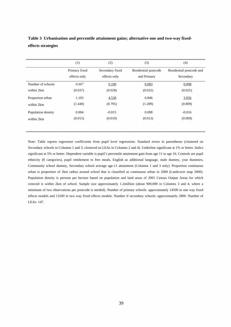
39

Table 3 Urbanisation and percentile attainment gains; alternative one and two-way fixed-

effects strategies

(1) (2) (3) (4)

Primary fixed

effects only

Secondary fixed

effects only

Residential postcode

and Primary

Residential postcode and

Secondary

Number of schools

within 2km

0.087

(0.037)

0.100

(0.028)

0.083

(0.032) 0.098

(0.025)

Proportion urban

within 2km

1.103

(1.440)

4.530

(0.795)

0.846

(1.289) 3.056

(0.809)

Population density

within 2km

0.004

(0.015)

-0.015

(0.010)

0.008

(0.013) -0.016

(0.009)

Note: Table reports regression coefficients from pupil level regressions. Standard errors in parentheses (clustered on

Secondary schools in Columns 1 and 3; clustered on LEAs in Columns 2 and 4). Underline significant at 1% or better. Italics

significant at 5% or better. Dependent variable is pupil’s percentile attainment gain from age 11 to age 16. Controls are pupil

ethnicity (8 categories), pupil entitlement to free meals, English as additional language, male dummy, year dummies,

Community school dummy, Secondary school average age-11 attainment (Columns 1 and 3 only). Proportion continuous

urban is proportion of 2km radius around school that is classified as continuous urban in 2000 (Landcover map 2000).

Population density is persons per hectare based on population and land areas of 2001 Census Output Areas for which

centroid is within 2km of school. Sample size approximately 1.2million (about 900,000 in Columns 3 and 4, where a

minimum of two observations per postcode is needed). Number of primary schools: approximately 14500 in one way fixed

effects models and 13200 in two way fixed effects models. Number if secondary schools: approximately 2800. Number of

LEAs: 147.

40

Table 4 Urbanisation and percentile attainment gains; geographical scope

- (1) (2) (3) (4) (5) (6) (7) (8) (9) (10)

Whole

sample

Primary school

low-density

Primary school

high-density

Low to high

density move

High to low

density move

Short

distance

move

Long

distance

move

Move not

within London

Move

within

London

Move

within

LEA

Move

outside

LEA

Number of

schools

within 2km

0.087

(0.037)

0.075

(0.029)

0.099

(0.029)

0.059

(0.036)

0.127

(0.028)

0.062

(0.035)

0.088

(0.023)

0.073

(0.019)

0.092

(0.036)

0.073

(0.019)

0.110

(0.029)

Proportion

urban

within 2km

1.103

(1.440)

-1.183

(1.300)

1.076

(0.936)

-0.158

(1.088)

1.658

(0.800)

0.288

(1.529)

0.732

(0.885)

1.672

(0.723)

-2.945

(1.982)

1.472

(0.712)

-0.294

(1.193)

Population

density

(per hectare)

0.004

(0.015)

-0.011

(0.010)

0.018

(0.011)

-0.011

(0.010)

0.008

(0.009)

0.004

(0.011)

0.003

(0.009)

-0.004

(0.007)

0.045

(0.016)

0.003

(0.007)

0.005

(0.011)

Sample 1201894 327949 274365 258946 323025 314728 302363 1049819 135130 1082839 119055

Note: Table reports regression coefficients from pupil level regressions. Standard errors in parentheses (clustered on Secondary school). Underline significant at 1% or better (Italics significant at

5%). Dependent variable is pupil’s percentile attainment gain from age 11 to age 16. Controls are pupil ethnicity (8 categories), entitlement to free school meals, English as additional language,

male dummy, Community school dummy, Secondary school average age-11 attainment, year dummies, Primary (age-11) school fixed effects. Proportion continuous urban is proportion of 2km

radius around school that is classified as continuous urban in 2000 (Landcover map 2000). Population density is persons per hectare based on population and land areas of 2001 Census Output

Areas for which centroid is within 2km of school. Low and high density refers to bottom (≤5) and top (≥13) quartile of schools within 2km. Low to high density is top quartile change (and vice

versa). Long and short distance refers to bottom (<0.9km) and top (>3.6km) quartile of distance between Primary and Secondary school attended.

Table 5 Urbanisation and pupil attainment; robustness of results

Percentile based on

mean

age-16 points

Acceleration in

attainment,

ages 11-14-16

Instrumental variable

estimates

(1) (2) (3) (4) (5) (6)

Levels Age-11 to

16 Diff

Double-

diff

Double-

diff

Age-11 to

16 Diff

Age-11 to

16 Diff

Number of schools

within 2km

-0.352

(0.029)

0 .082

(0.017)

0.098

(0.023)

0.067

(0.024)

0.205‡

(0.108)

[0.122]

0.181

(0.113)

[0.123]

First Stage Statistics

F-Statistics - - - - 210.40

(0.0000)

198.41

(0.0000)

Hansen Statistics

(p-value)

- - - - 3.515

(0.319)

2.740

(0.4335)

Pupil characteristics No Yes Yes Yes Yes Yes

Primary school effects No Yes Yes Yes Yes Yes

Secondary school

average peer

achievement

No Yes No Yes Yes Yes

Postcode Area effects No No No No No Yes

Note: Table reports regression coefficients from pupil level regressions. Standard errors in parentheses (clustered on

Secondary school, expect Columns 5 and 6). Underline significant at 1% or better (‡ significant at 6%). Dependent variable

is pupil’s percentile gains from age 11. Controls are pupil ethnicity (8 categories), entitlement to free school meals, English

as additional language, male dummy, Community school dummy, Secondary school average age-11 attainment, year

dummies. Sample size approximately 1.2million (Columns 1 to 4). Instrumental variable in Columns 5 and 6 for London

metropolitan area only; sample size about 140,000 observations. Instruments are: residential postcode distance from closest

tube station and to closest rail station within 2km, plus dummies for no rail station and no train station within 2km of

residential postcode. Column 6 additionally controls for postcode area fixed effects. First stage statistics from models with

standard errors clustered at the postcode level (p-values in round brackets); second stage standard errors clustered at

postcode level in round brackets and at the Secondary school level in square brackets.

41

Table 6 Urbanisation and percentile attainment gains; resources, policy interventions

and school competition

(1) (2) (3) (4) (5) (6)

All schools All schools All schools Community

only

Non-

community

All schools

Number of state

Secondary schools

within 2km

0.363

(0.101)

0.363

(0.101)

0.374

(0.102)

0.250

(0.131)

0.439

(0.168)

0.332

(0.109)

Number of state Primary

schools

within 2km

0.016

(0.044)

0.005

(0.044)

0.005

(0.045)

-0.003

(0.052)

-0.005

(0.069)

-0.026

(0.046)

Number of qualified

teachers (FTE)

- 0.065

(0.017)

0.066

(0.017)

0.066

(0.019)

0.044

(0.029)

0.064

(0.017)

Number of pupils x100

(FTE)

- -0.321

(0.104)

-0.324

(0.104)

-0.302

(0.110)

-0.155

(0.186)

-0.321

(0.103)

Expenditure per pupil in

Local Education

Authority (£00s)

- 0.080

(0.034)

0.093

(0.041)

0.095

(0.039)

0.036

(0.059)

0.074

(0.034)

Number of Beacon

Secondary schools

- - - - - 0.039

(0.306)

Number of Beacon

Primary schools

- - - - - 0.419

(0.160)

Number of Independent

Secondary schools

- - - - - -0.106

(0.083)

Number of Independent

Primary schools

- - - - - 0.037

(0.120)

Urban land cover and

population density

Yes Yes Yes Yes Yes Yes

Urban school policies No No Yes No No No

Primary school fixed

effects

Yes Yes Yes Yes Yes Yes

Note: Table reports regression coefficients from pupil level regressions. Standard errors in parentheses (clustered on

Secondary school). Underline significant at 1% or better (Italics significant at 5%). Dependent variable is pupil’s percentile

attainment gain from age 11 to age 16. Controls are pupil ethnicity (8 categories), entitlement to free school meals, English

as additional language, male dummy, Community school dummy, Secondary school average age-11 attainment, year

dummies, Primary (age-11) school fixed effects. FTE means full time equivalent. Column 6 also controls for whether current

Secondary is a Beacon. Regressions in Columns 4 and 5 are run separately for pupils in Community Secondary schools and

pupils in Secondary schools other than Community (Voluntary Controlled, Voluntary Aided and Foundation). Sample size

approximately 1.2million (approximately 801,000 in Column (4) and 400,300 in Column (5)).

42

APPENDIX

Estimation of Two-Way Fixed Effects

The main challenge to estimating the two-way fixed effects models described by equation (3)

in section 0 is the large number of school and postcode fixed effects that need to be estimated

or eliminated, especially when we have a large number of pupil observations.

In the data for England (described above) we have over 14000 Primary schools, over 2800

Secondary schools, around 500000 postcodes, and data on over 1.2 million pupils. The

simplest approach to estimating the full model would be to include either the 2800+

Secondary school or the 14000+ Primary school dummies as regressors, and de-mean the data

using a within-groups transformation to eliminate home postcode fixed effects. Since this is

infeasible on the full dataset of pupils, we follow a procedure inspired by a series of papers

by Abowd and co-authors (Abowd and Kramarz, 1999, Abowd Kramarz and Margolis, 1999,

and Abowd, Creecy and Kramarz, 2002) for firm and individual effects. Our approach

involves, as a first stage, using this estimator on sub-groups (A) of the full data set in order to

estimate the postcode fixed effects for each sub-group. When this is complete, we use the full

sample to re-estimate the model, using the either within-Primary or within-Secondary school

transformation on a model that includes the postcode fixed effects estimated from the first

stage as a regressor.

More formally, consider the case of Primary and residential postcode fixed effects; we

estimate:

(4)

δβ

υδβˆ'ˆˆ

,)''()(

,

,,,,

lsk

ljk

ljkil

jkilsksk

ljkijk

ljkijki

duyn

Aidduuyy

+Δ−Δ=

∈+−+Δ−Δ=Δ−Δ

for all subgroups A (defined below); then, on the full data set:

(5)jki

jll

jjkijk

jjkijki nnuuyy ,,,, )ˆˆ()( ωθβ +−+Δ−Δ=Δ−Δ

43

Ideally, each subgroup A would be defined such that that it includes all pupils living in a

specific set of postcodes R, who all attend Primary schools within a set P, to which no other

pupils (other than those in R) are admitted. All the relevant postcode and Primary fixed

effects could then be estimated consistently for each of these ‘autarchic’ systems using only

data from pupils in each subgroup A.

In practice, school admissions systems are not so cleanly defined, but the process of

identifying suitable groups is aided by the fact that admission in England is organised

geographically by Local Education Authorities (LEAs). In most cases, pupils attending a

school within a given LEA come from neighbourhoods within that LEA, or from a closely

neighbouring LEA. So we form sub-groups A on an LEA-by-LEA basis and proceed using

the following steps:

(a) For a given LEA L, draw all pupils who live in the set of postcodes R in that LEA,

plus all pupils in a set Primary schools P which intersects the set R through pupil

Primary school choice, i.e. pupils in a set of postcodes Q outside the LEA L, going

to the same set of Primary schools P as pupils in R.

(b) Estimate (4) on this sub-sample of pupils (sub-group A), using dummy variables for

the Primary schools P, allowing for postcode fixed effects for the postcode set R

plus the set Q of postcodes that intersect with P through pupil Primary school

choice, but are outside the LEA.

(c) Retrieve estimates for the postcode fixed effects for the set R, i.e. in (4). ln̂

(d) Repeated for each LEA until all postcode fixed effects have been estimated.

(e) Estimate (5) using the full England sample and the estimated postcode effects from

step (c).

Note that this is an approximate method, because at step (b) we have not used data on all

pupils in the set of postcodes Q that are outside the LEA in order to compute the fixed effects

Q. However, these postcode fixed effects will be estimated consistently if pupils in the set

44

Q P∩ are a random sample of all pupils living in postcode Q. Moreover, we do not use the

estimates of effects Q in the last stage (e), but re-estimate them when we reach the LEA in

which they are located during step (d). So, the only concern is that not estimating Q correctly

(i.e. on the full set of pupils living in those postcodes) may bias our estimates of the Primary

school effects P, which in turn could affect our estimates of postcode effects R. We checked

the sensitivity of the results to these sorts of problems by re-defining our group A in various

ways, for example by excluding Q completely and using only the sample of pupils in R. A

similar method can be used to control for residential postcode and Secondary school fixed

effects.

45