Upstream River Responses to Low Head Dam Removal

by

Robert Alan Amos

A thesis presented to the University of Waterloo

in fulfillment of the thesis requirement for the degree of

Master of Applied Science in

Civil Engineering

Waterloo, Ontario, Canada, 2008

© Robert A. Amos 2008

ii

Author’s Declaration

I hereby declare that I am the sole author of this thesis. This is a true copy of the thesis, including any required final revisions, as accepted by my examiners. I understand that my thesis may be made electronically available to the public.

iii

ABSTRACT

Field and modelling investigations of eight failed or removed dams have been undertaken

to examine the upstream effects of low head dam decommissioning on channel

morphology. Failed or decommissioned sites were selected such that no upstream

interventions or channel mitigation had been applied since the time of decommissioning

resulting in a physically-based analog consistent with the passive dam removal

restoration approach. Field surveys of the sites, which failed between 2 years and 70

years ago, included longitudinal profiles, cross-sections and bed material pavement

sampling on each riffle, run, and headcut.

Findings demonstrate that vertical disturbances typically in the form of headcuts

frequently extend well beyond the backwater limits of most reservoirs. Although in most

cases, critical velocity and shear stress thresholds were exceeded, the localized increases

in friction slope where headcuts occurred demonstrated that the velocities associated with

larger flows exceeded critical thresholds more often than critical shear stress thresholds.

Findings show that if the grain size distributions of the underlying alluvial geologic units

are close to that of critical velocity thresholds, when headcuts are initiated (with their

resulting increase in friction slope), they can result in continued channel degradation

upstream of impoundment regions.

iv

Acknowledgments I would like to thank my supervisor Dr. Bill Annable for teaching me the process of academic excellence associated with field based research. Thanks for instilling in me the values of this process found through hard work, many hours, and many, many revisions. I would like to thank my dear friends and research colleagues for assisting me with the countless hours of field work. Whether it was walking kilometers upstream through the thalweg, digging rocks out of the water and backpacking them out, or getting up before the sun for an early start, your enthusiasm and interest was incredible. Thanks to: Mason Marchildon, Terry Ridgway, Pete Thompson, Laddie Kuta, and Mike Fabro. The support from my family and dearest girlfriend Danielle has kept me grounded in life outside of school. Thanks so much for your love and compassion. Lastly, thanks to my roommate the Gaffer. What fun!

v

Table of Contents 1 INTRODUCTION ...................................................................................................... 1 2 BACKGROUND ........................................................................................................ 5

2.1 Rationales for Dam Removal.............................................................................. 5 2.2 Methods of Dam Removal .................................................................................. 7

2.2.1 Removal Alternatives of the Physical Barrier ............................................ 9 2.2.2 Impoundment Composition and Remediation Considerations ........................ 11

2.3 Upstream Geomorphic and Hydraulic Responses Following Passive Dam Removal ........................................................................................................................ 13

2.3.1 Modes of Headcut Migration .................................................................... 21 2.3.2 Lateral Migration of Channels Following Dam Removal ........................ 27

2.4 Sediment Transport and Tractive Force Analysis............................................. 29 2.5 Longitudinal Hydraulic and Sedimentological Channel Evolution Responses to Passive Dam Removal .............................................................................................. 35

3 FIELD AND ANALYSIS METHODS .................................................................... 44 3.1 Field Surveys .................................................................................................... 46

3.1.1 Longitudinal Profiles ................................................................................ 47 3.1.2 Cross-Sectional Profiles............................................................................ 48 3.1.3 Sediment Sampling ................................................................................... 49

3.2 Numerical Analysis Methods............................................................................ 53 3.2.1 Discharge Frequency Estimates....................................................................... 56 3.2.3 Tractive Force and Permissible Velocity Analysis................................... 61

4 RESULTS AND DISCUSSION............................................................................... 63 4.1 Upstream Disturbance Propagation .................................................................. 63 4.2 Power, Velocity and Shear Profiles .................................................................. 65 4.3 Tractive Force and Velocity Results................................................................. 77

5 CONCLUSIONS and RECOMMENDATIONS ...................................................... 89 5.1 Recommendations............................................................................................. 90

6.0 References............................................................................................................. 91 Appendix A: Croton Dam on Big Creek at Delhi............................................................ 98 Appendix B: Hawkesville Dam on Conestoga River at Hawkesville............................ 105 Appendix C: Huttonville Dam on Credit River at Huttonville ...................................... 111 Appendix D: Chilligo Dam on Ellis Creek at Cambridge ............................................. 119 Appendix E: Greenfield Dam on Nith River at Greenfield ........................................... 126 Appendix F: Sutton Dam on Patterson Creek at Simcoe............................................... 132 Appendix G: Teeswater Dam on Teeswater River at Teeswater................................... 137 Appendix H: Bognor Dam on Walter’s Creek at Bognor.............................................. 145

vi

List of Tables

Table 1. Approximate threshold conditions for granular material by particle size

(modified from Julien, 1995) .................................................................................... 33 Table 2. List of dam study sites, river names, valley slope and dominant upstream

physiography............................................................................................................. 45 Table 3. General channel bed grain size distributions based upon the median bed-

material particle size (after Bunte and Abt, 2001). ................................................... 53 Table 4. Flood flow frequency each site.......................................................................... 59 Table 5. Summary of bed material and sizes, exceeding critical shear stress thresholds

for QBF, Q2, and Q20 within and upstream of site impoundments. Note: if particle sizes are identified in the table, they exceed critical thresholds at one or more morphological features.............................................................................................. 86

Table 6. Summary of bed material, and sizes, exceeding critical velocity thresholds for QBF, Q2, and Q20 within and upstream of site impoundments. Note: if particle sizes are identified in the table, they exceed critical thresholds at one or more morphological features.............................................................................................. 86

vii

List of Figures

Figure 1. Rationales for dam removals in the U.S.A. (modified from Pohl, 2002)........... 6 Figure 2. Proposed systematic approach for dam removal decision making..................... 9 Figure 3. Dam removal using staged reduction. .............................................................. 10 Figure 4. Typical reservoir sedimentation pattern (modified from Julien, 1995)............ 11 Figure 5. Three scenarios founding abrupt change in channel invert following dam

removal. .................................................................................................................... 14 Figure 6. a) Cross-sectional and b) longitudinal upstream evolution of channel

morphology through a reservoir following dam removal (modified from Doyle et al., 2002). ........................................................................................................................ 15

Figure 7. Average channel velocity profiles for increasing discharge within each stage of the channel evolution model suggested by Doyle et al., 2002. QBF, Q2, Q20, Q50, Q100 values represent the bankfull, 2-year, 20-year, 50-year, and 100-year discharge frequency magnitudes respectively........................................................................... 18

Figure 8. Derivation of total sediment load surcharge curve to predict effective discharge (modified from Biedenharn and Copeland, 2000). ................................................... 20

Figure 9. The influence of various combinations of resistant and nonresistant bed material on headcut migration (modified from Bush and Wolman, 1960)............... 22

Figure 10. The physical parameterization of a of a headcut profile (modified from Begin et al., 1980). .............................................................................................................. 24

Figure 11. Modes of headcut migration for a) rotating headcuts and b) stepped headcuts (modified from Stein and Julien, 1993). ................................................................... 26

Figure 12. Channel centreline migration over time to define channel activity (modified from Shields et al., 2000).......................................................................................... 28

Figure 13. Relation of applied and resisting forces on a particle resting on a supporting surface (modified from Leopold et al., 1964). .......................................................... 30

Figure 14. Shields particle motion diagram (modified from Julien, 1995). .................... 31 Figure 15. Bed surface for nonuniform grain size mixtures (modified from Julien, 1995).

................................................................................................................................... 34 Figure 16. Comparison of different hiding functions (modified from Shvidchenko et al.,

2001). ........................................................................................................................ 35 Figure 17. Typical a) unit stream power, b) average channel velocities, and c) main

channel velocities for the five stages of channel evolution after Doyle et al. [2002] for a discrete range in flows between bankfull (QBF) and the 100-year (Q100) magnitude discharge events. ..................................................................................... 39

Figure 18. Typical a) average channel shear and b) main channel shear for the five stages of channel evolution after Doyle et al. [2002] for a discrete range in flows between bankfull (QBF) and the 100-year (Q100) magnitude discharge events........................ 40

Figure 19. Typical a) unit stream power, b) averge channel velocities, and c) main channel velocities for the five stages of channel evolution after Doyle et al. [2002] for 100 different incremental discharges between 0 < Q < Q100............................... 42

Figure 20. Typical a) average channel shear and b) main channel shear for the five stages of channel evolution after Doyle et al. [2002] for 100 different incremental discharges between ................................................................................................... 43

viii

Figure 21. Locations of study sites within Southern Ontario. ......................................... 45 Figure 22. Example plan view of a field survey of Teeswater River at Teeswater. ........ 47 Figure 23. Longitudinal profile of Teeswater River at Teeswater................................... 48 Figure 24. Locations of bed material samples along a riffle............................................ 50 Figure 25. Locations of bed material samples along a headcut. ...................................... 50 Figure 26. Example pavement sample distributions of the uppermost riffle (Riffle 1) of

Credit River at Huttonville........................................................................................ 52 Figure 27. Comparison of a) HEC-RAS calibrated vs. regional analysis method for

bankfull discharge and b) adjusted Manning’s roughness coefficient vs. estimated Manning’s roughness coefficient using Limerinos [1970]. ...................................... 56

Figure 28. Conestoga River at Hawkesville sub-watershed DEM within the Upper Grand River watershed. ....................................................................................................... 58

Figure 29. Comparison of yearly instantaneous maximum discharges, Weibull Plotting Position, Log Pearson-III Analysis, Gingras et al. [1994] and Annable [1996] methods of discharge estimation for the Q1.5, Q2, Q20 and Q100 return periods for Environment Canada gauge stations proximal to study sites at a) Big Creek near Delhi (02GC006) b) Conestoga River at Glen Allan (02GA028) and c) Credit River at Norval (02HB025). ............................................................................................... 60

Figure 30. Ratio of maximum upstream headcut extent to normalized reservoir limit. .. 64 Figure 31. Results of a) unit stream power, b) average velocity, c) main channel velocity

for incremental discharge analyses between 0 < Q < Q100, and d) thalweg elevation along the longitudinal profile for the Credit River at Huttonville (site 3). ............... 67

Figure 32. Results of a) average channel shear stress and b) main channel shear stress for incremental discharge analyses ranging between Q < Q < Q100 along the longitudinal profile for the Credit River at Huttonville (site 3)................................ 68

Figure 33. Average channel velocities of a stable upstream cross-section and the envelope of incised channel cross-sections for discharges ranging between Q < Q < Q100 for the Credit River at Huttonville (site 3). ....................................................... 68

Figure 34. Main channel velocities of a upstream stable cross-section and the envelope of incised cross-sections for discharges ranging between Q < Q < Q100 for site 3. 70

Figure 35. Results of unit stream power of flows which overtop banks vs. normalized longitudinal channel profile distance. ....................................................................... 73

Figure 36. Results of a) average channel velocity and b) main channel velocity of flows which overtop banks vs. normalized longitudinal channel profile distance.. ........... 74

Figure 37. Results of a) average channel shear and b) main channel shear of flows which overtop banks vs. normalized longitudinal channel profile distance........................ 75

Figure 38. Results of a) main channel shear vs. tc50 threshold and b) main channel shear vs. tc 84 threshold along the normalized longitudinal profile at QBF. ....................... 78

Figure 39. Results of a) main channel shear vs. tc 50 threshold and b) main channel shear vs. tc 84 threshold along the normalized longitudinal profile at Q2.......................... 79

Figure 40. Results of a) main channel shear vs. tc 50 critical threshold and b) main channel shear vs. tc 84 critical threshold along the normalized longitudinal profile at Q20. ............................................................................................................................ 80

ix

Figure 41. Results of a) maximum permissible particle size at QBF vs. the range of measured d50 values and b) maximum permissible particle size at QBF vs. the range of measured d84 values along the normalized longitudinal profile. .......................... 81

Figure 42. Results of a) maximum permissible particle size at Q2 vs. the range of measured d50 values and b) maximum permissible particle size at Q2 vs. the range of measured d84 values along the normalized longitudinal profile................................ 82

Figure 43. Results of a) maximum permissible particle size at Q20 vs. the range of measured d50 values and b) maximum permissible particle size at Q20 vs. the range of measured d84 values along the normalized longitudinal profile. ......................... 83

x

Notation Symbol Unit Description a [-] sediment rating curve regression fitting parameter A [L2] channel cross-sectional area A' [-] empirical coefficient b [-] sediment rating curve regression fitting parameter B [M L-3] soil bulk density ds [L] particle size di [L] particle size where i denotes percentage finer C [-] coefficient of friction DA [L2] effective drainage area E [M L-2T -1] detachment rate per unit area f [-] Darcy-Weisbach friction factor

FN [M LT-2] force normal to the bed slope

FO [M LT-2] fricitonal stress opposing motion F [-] Froude number g [L T -2] acceleration due to gravity G [-] specific gravity of bed material h [L] initial drop height of the headcut hn [L] normal flow depth hu [L] flow depth at the crest of the headcut P [M L1T-1] stream power [M T-1] unit stream power

QBF [L3 T -1] bankfull discharge

Qi [L3 T -1] observed discharge

QEFF [L3 T -1] effective discharge

QF [L3 T -1] channel forming discharge

QSi [M T -1] sediment transport rate related to discharge Qi

qs [M L-1T -1] rate of sediment transport per unit width Qs [L3 T -1] bed material discharge R [L] hydraulic radius Rc [L] radius of curvature Sf [-] friction slope Sv [-] valley slope So [-] bed slope

P

xi

t [T] time interval T [L] top width of channel discharge Td [T] time for the impingement scour to develop horizontally and

reach the toe of the vertical face

Tu [T] time for upstream vertical scour to reach the toe of the vertical face

u* [L/T] shear velocity V [L T -1] flow velocity

vm [L T -1] kinematic viscosity of fluid W [L] top width of bankfull channel x [L] distance along the channel y [L] elevation Yo [L] constant elevation by which the baselevel is lowered at x = 0 Greek Λ [L] wetted perimeter ξ [-] empirical coefficient

ρm [M L-3] fluid density (1000kg/m3) t* [dimensionless] Shield's parameter tC [M L-1T -2] critical shear strength to [M L-1T -2] shear at the bed

γs [M L-2T -2] bulk unit weight of the sediment (2650 kg/m3)

γw [M L-2T -2] specific weight of water (9810 kg/m3) Ø [-] critical angle of repose Ω [-] sinuosity

1

1 INTRODUCTION Dams have been integral to the advancement of mankind for hundreds of years by

providing sources of power, water supply, flood control, irrigation, and navigation;

amongst many other uses. Correspondingly, the siting and construction of dams have

segmented the majority of rivers in the Northern Hemisphere resulting in large-scale

environmental disruption (Dynesius, 1994). The environmental impacts dams can have

on their surrounding physical and biological environments are well documented (Petts,

1984; Ligon, 1995; Bednarek, 2001).

In more recent times, the removal of dams has garnered considerable attention; primarily

related to structures which are no longer fulfilling their primary design purpose. The

acceleration in structure removals reflects expiring life expectancies, the desire to restore

ecological connectivity, and national policies directed at mitigating environmental

impacts of riverine structures. Several studies have also been focused on the

ecological effects, sediment transport responses, and channel adjustments downstream of

impoundments post removal (Dynesius, 1994; Ligon, 1995; Pansic et al., 1998; Dolye et

al., 2003; Doyle, 2005; Cui et al., 2005; Ashley, 2006).

In general, dam restoration projects consist of removing the physical barrier and the re-

establishment of a stable channel; floodplain; and sediment continuity within the

impoundment footprint. There are two typical approaches to channel recovery which are

commonly referred to as active and passive restoration. Active restoration entails the

design and construction of a river channel to either it’s historical or new stable channel

2

morphology and removing the impounded sediments to pre-dam topographic conditions.

Passive restoration involves channelization through the impoundment sediments via

initiating erosional processes (i.e. headcuts) at the dam face to form a channel. Over time

with the upstream propagation of headcuts, an incised channel forms through the

impoundment sediments, which, eventually tends toward a state of dynamic morphologic

stability. The active restoration strategy, however, is notably more costly than the passive

approach rendering the passive approach to often being the preferred remediation

alternative.

The passive restoration approach, however, can have several negative impacts to the local

ecology and river stability if not properly considered and mitigated in the design and

construction process. Headcuts initiated at the dam face migrate upstream to achieve

base level lowering within the impoundment and initially create an incised channel. The

scale of the headcuts, and associated incision, is dependent upon the extent of base level

lowering necessary to achieve channel stability in addition to establishing discharge and

sediment continuity between the upstream and downstream reaches of the impoundment.

Incised channels, of which headcuts are a physical identifier, have distinctive

characteristics which affect the hydraulic, sedimentological and geomorphical processes

and typically indicate periods of channel instability or disequilibrium (Simon and Darby,

1999). An incised channel typically has increased bank heights and enlarged cross-

sections with increased channel discharge capacity relative to a bankfull channel and

flood plain dominated morphology. The incised channel morphology results in higher

shear stresses; velocities; and unit stream power during moderate to high flood flows as

3

the floodplain is rendered inaccessible (Simon, 1998). Consequently, an excess of

sediment transport capacity occurs within the incised channel reaches relative to the

amount of sediment supplied. This initiates an increased sediment yield within the

incised channel (i.e. within the reservoir impoundment) to the downstream reaches. This

degradational process can affect the impoundment and downstream reaches over several

years until dynamic channel stability is attained and often results in declines of both

hydraulic and ecosystem function (Shields et al., 2000; Beechie et al., 2007). The

degradational processes can also have socio-economic ramifications resulting from land

loss, the undercutting of bridges, road crossing or other man made structures.

It is commonly believed that headcuts and channel incision related to the passive

restoration approach diminish in size and terminate at the upstream extent of the

impoundment. However, depending upon such factors as headcut size, headcut slope,

local hydraulic grade lines, local geology, geometric characteristics, and flood forming

flows, headcuts may continue to migrate beyond the upstream limits of the impoundment.

Therefore, the act of inducing headcuts at the dam face to initiate a passive restoration

strategy may have upstream effects well beyond the intended limits of the reservoir

impoundment leading to continued channel degradation.

The purpose of this study is to examine if channel disturbances related to the

decommissioning of low head dams exist, utilizing the passive restoration approach,

upstream of reservoir impoundments. If channel disturbances are found, a secondary

objective of this work is to provide remediation strategies to mitigate such upstream

4

disturbances. As there are a limited number of dam restoration projects with sufficient

time lines to study the effects of upstream channel degradation, an examination of

channel morphologies and evolutions using the analog of removed or failed dams with no

upstream interventions to the headcut driven channel formation processes will be studied.

As channel evolution is dependent upon numerous criteria such as local geology, valley

slopes, particle sizes and gradations, reservoir sediment levels and channel forming flow

depths, failed or removed dams will be studied on a broad spectrum of environmental

factors.

5

2 BACKGROUND The literature review provided within this thesis is assembled into the following sections:

• Rationales for dam removal;

• Methods of dam removal;

• Geomorphic and hydraulic responses to channelization through reservoir

impoundments;

• Tractive force analysis; and

• Longitudinal channel evolution responses to dam removal.

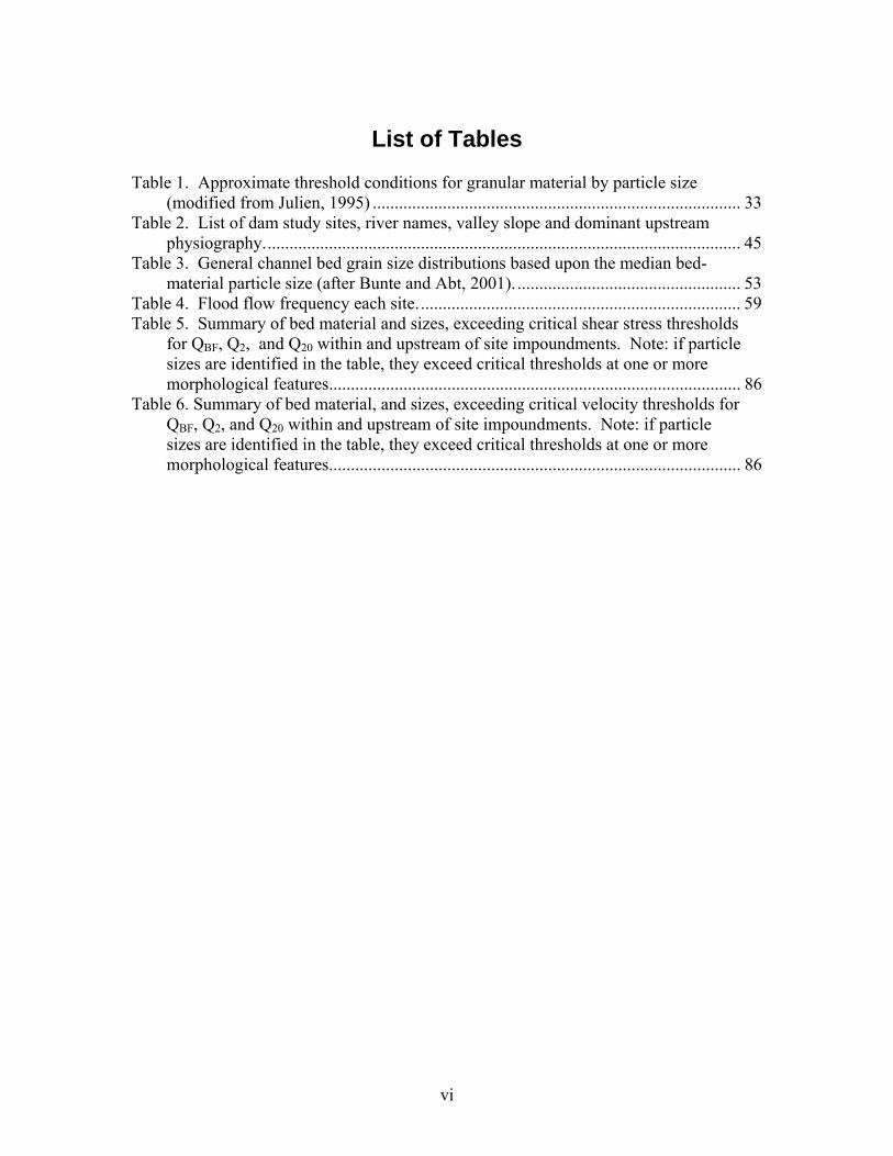
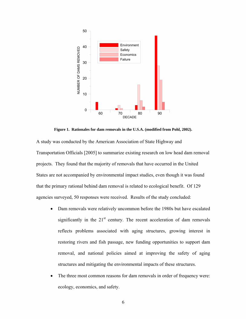
2.1 Rationales for Dam Removal Pohl [2002] compiled a database of dams within the U.S.A. and analyzed both spatial and

temporal trends in dam removal strategies. Pohl found that dam removal initiatives were

strongly related geographically to ecological values and funding opportunities for the

dismantling of structures. Four principle motivations were identified: environmental

initiatives to re-establish riparian corridor connectivity, dam safety, economics, and dam

failures. Pohl [2002] also identified an escalation of dam removals in the 1990s, as

illustrated in Figure 1, for environmental reasons due to social and environmental policy

changes.

6

60 70 80 90DECADE

0

10

20

30

40

50

NU

MB

ER

OF

DAM

S R

EMO

VE

D

EnvironmentSafetyEconomicsFailure

Figure 1. Rationales for dam removals in the U.S.A. (modified from Pohl, 2002).

A study was conducted by the American Association of State Highway and

Transportation Officials [2005] to summarize existing research on low head dam removal

projects. They found that the majority of removals that have occurred in the United

States are not accompanied by environmental impact studies, even though it was found

that the primary rational behind dam removal is related to ecological benefit. Of 129

agencies surveyed, 50 responses were received. Results of the study concluded:

• Dam removals were relatively uncommon before the 1980s but have escalated

significantly in the 21st century. The recent acceleration of dam removals

reflects problems associated with aging structures, growing interest in

restoring rivers and fish passage, new funding opportunities to support dam

removal, and national policies aimed at improving the safety of aging

structures and mitigating the environmental impacts of these structures.

• The three most common reasons for dam removals in order of frequency were:

ecology, economics, and safety.

7

• Most of the dams removed have a structural height smaller than six meters.

This is in agreement with observations made by the Heinz Center [2002]. The

majority of low head dams (79%) were completely removed with the

remaining structures either being breached or partially removed. Further, the

study found that the deconstruction cost typically accounted for approximately

50% of the total removal cost, where the remaining costs were related to

sediment management, stream channel restoration and monitoring.

Public reaction to dam removal is often quite varied. Commonly, a portion of the public

opposes removal based upon issues such as loss of recreation opportunities, reduced

access to aquatic environments, alteration of aesthetic parameters, private land owner

concerns, loss of cultural or historic values, and costs related to removal. In contrast,

support is often found for environmental enhancements to water quality and fish

migration, along with residents and government agencies concerned with dam safety,

liability and litigation (Canadian Dam Association, 2005).

2.2 Methods of Dam Removal

Standard methods and/or generic guidelines do not exist for the removal of dams and

reservoir restorations; similar to the state of the science for river restoration (Copeland et

al., 2000). In order to achieve the desired effects from dam removal; be it related to

environmental restoration, minimizing public health and safety risks, reducing liability,

or minimizing maintenance costs to dam owners, dam removal is highly site specific and

8

techniques must vary to suit the socio-economic, local ecological and geomorphologic

conditions.

Socio-economic considerations include the funding sources for dam removal, the

impending risk and liability of dam failure, public support or protests, public safety,

functionality, and ownership. Ecological aspects consider changes in: flow regime; water

temperature; sediment and pollutant releases and super-saturations; aquatic habitats; and

the migration of fish and other aquatic organisms. The geomophological implications

include: downstream sedimentation and upstream erosion; channelization through the

impoundment; bank stability; lateral and transverse channel adjustment and degradation;

and attaining a natural channel in a state of quasi-equilibrium for the given surrounding

geology and valley slopes.

Although many of the socio-economic, ecological and geomorphological considerations

overlap in a dam removal project, they are seldom congruent (Bednarek, 2001). The

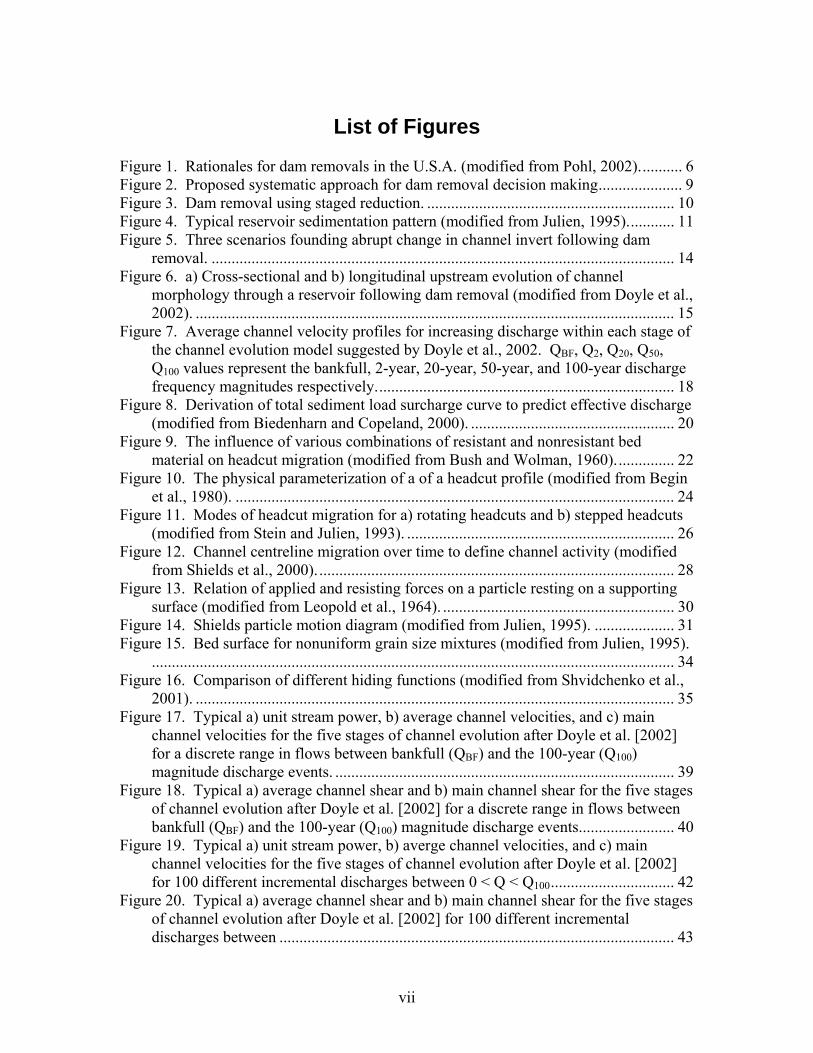
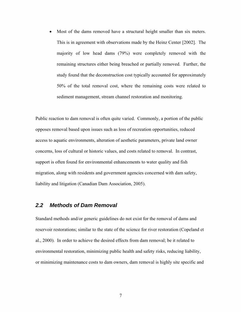
Heinz Center [2002] developed a systematic approach to assess the feasibility of a dam

removal. This approach establishes goals, identifies major issues of concern and assesses

potential outcomes of the river ecology and morphology as outlined in Figure 2.

9

Step 1: Define goals and objectives

For keeping dam:Water supplyIrrigationFlood controlHydroelectric powerNavigationFlat-water recreationWaste disposal

For removing dam:Safety & security considerationsLegal & liability concernsRecreationSite restorationEcosystem restorationWater quality

Step 2: Identify major issues of concern

Safety & Security

Social

Environment

Economic

Legal

Management

Step 3: Collect and assess data

Physical Biological Legal Social Economic

Step 4: Decision making

Leave in place Remove

Step 5: Dam Removal

Step 6: Data collection, assessment, and monitoring

Figure 2. Proposed systematic approach for dam removal decision making

(after Heinz Center, 2002).

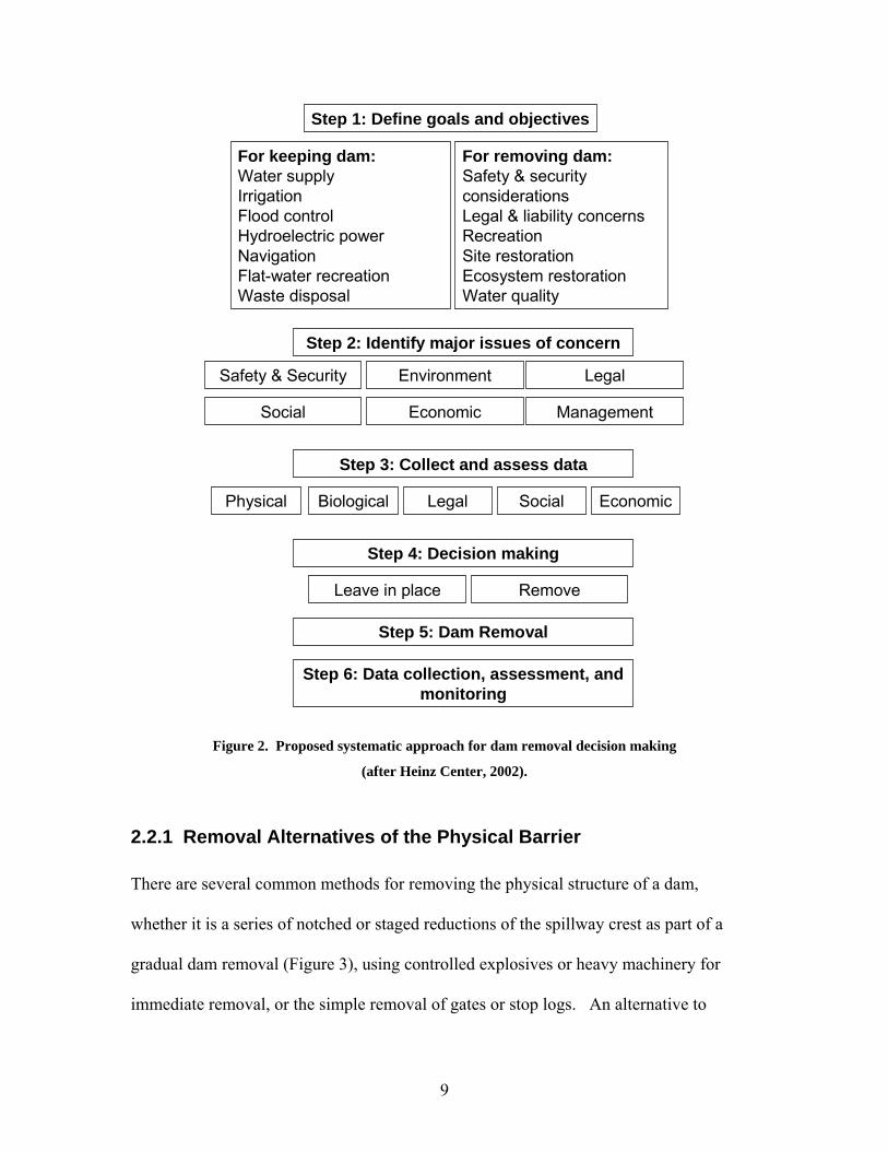
2.2.1 Removal Alternatives of the Physical Barrier

There are several common methods for removing the physical structure of a dam,

whether it is a series of notched or staged reductions of the spillway crest as part of a

gradual dam removal (Figure 3), using controlled explosives or heavy machinery for

immediate removal, or the simple removal of gates or stop logs. An alternative to

10

removing the physical barrier is to divert the river around the dam completely if sufficient

land is available.

Stage I. Pre-removal Stage II. Dewatering stage

Stage III. Initial channel incision

Stage IV - n. Stages removed until complete

Underlying geologic unit

Impacted Sediment

Figure 3. Dam removal using staged reduction.

Removals can also be limited to partial removal or dam breaches if complete removal is

deemed not to be the preferred option. In these scenarios, the majority of the physical

structure is left intact, and either a vertical notch is cut through the entire height of the

dam face (typically consistent with the downstream bankfull channel width) or the height

of the spillway is reduced to the upstream height of the deposited sediments. Partial

removal is often considered a preferred restoration alternative to avoid the costs of full

removal, to stabilize upstream reservoir sediments (particularly if contaminated sediment

concerns exist), and to retain some structure for historic or cultural purposes.

11

2.2.2 Impoundment Composition and Remediation Considerations

Dams affect the transport of both sediment and organic material. Upon construction of a

dam, channel velocities decrease approaching the dam face, the gradually varied flow

profile depicts an M1 profile for a mildly sloping channel, and a reduction in sediment

transport capacity results. Sediments entering a reservoir commonly deposit throughout

its full length, both raising the bed elevation and reducing the channel bed slope over

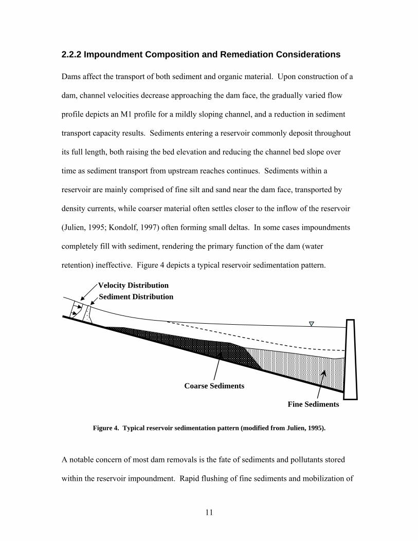
time as sediment transport from upstream reaches continues. Sediments within a

reservoir are mainly comprised of fine silt and sand near the dam face, transported by

density currents, while coarser material often settles closer to the inflow of the reservoir

(Julien, 1995; Kondolf, 1997) often forming small deltas. In some cases impoundments

completely fill with sediment, rendering the primary function of the dam (water

retention) ineffective. Figure 4 depicts a typical reservoir sedimentation pattern.

Figure 4. Typical reservoir sedimentation pattern (modified from Julien, 1995).

A notable concern of most dam removals is the fate of sediments and pollutants stored

within the reservoir impoundment. Rapid flushing of fine sediments and mobilization of

Fine Sediments

Coarse Sediments

Sediment Distribution Velocity Distribution

12

potential pollutants accumulated from the impoundment region upstream of the dam face

to downstream channel reaches may cause considerable channel aggradation and have

severe ecological and water quality effects (Wohl, 2000). Cheng and Granata [2004] also

identifies that the downstream release of sediments can have prohibitive effects upon

infrastructure and water intakes.

A primary objective of dam restoration is to minimize sedimentation to downstream

reaches. This is commonly achieved within the impoundment region by developing a

dynamically stable channel and floodplain using one of two general methods. The first

method considers the construction of a channel and floodplain within the impoundment

region consistent with the historical topography and / or stable upstream morphology by

excavating a channel and the preponderance of the sediments to the pre-dam conditions.

This is referred to as the active channel recovery method (Stanley and Doyle, 2002; Selle

et al., 2007). The active channel recovery method typically requires sizable

investigations (both spatially and temporally), engineered designs, and often significant

disposal fees for contaminated sediments and construction costs that often render this

alternative financially prohibitive.

An alternative approach, commonly referred to as the passive channel recovery method

(Stanley and Doyle, 2002; Selle et al., 2007) does not require the removal of the entire

structure or impounded sediments. This approach entails channelization through the

impoundment sediments while leaving the majority of deposited material in place, and

allows a channel to evolve to a state of quasi-equilibrium (Leopold et al., 1964) with

13

time. Although a channel can be constructed through the impoundment sediments using

natural channel design techniques, the passive method typically subscribes to the

initiation of headcuts at the dam face (via notches in the dam face) resulting in a channel

evolving through the impoundment sediment with time tending towards a state of quasi-

equilibrium. This approach utilizes little, if any, mechanical means of channel

construction and relies solely upon the migration of a headcut or headcuts to recreate the

channel and associated floodplains. In turn, the dispositions of impounded sediments rely

solely on downstream conveyance and depositional patterns (Selle et al., 2007). If the

rate and volumes of downstream sedimentation can be controlled while meeting the

remaining objectives of the project, the passive approach garners considerable interest as

a cost effective remediation alternative.

2.3 Upstream Geomorphic and Hydraulic Responses Following

Passive Dam Removal

The focus of the discussion herein will consist of the upstream hydraulic,

sedimentological and geomorphological outcomes of passive impoundment

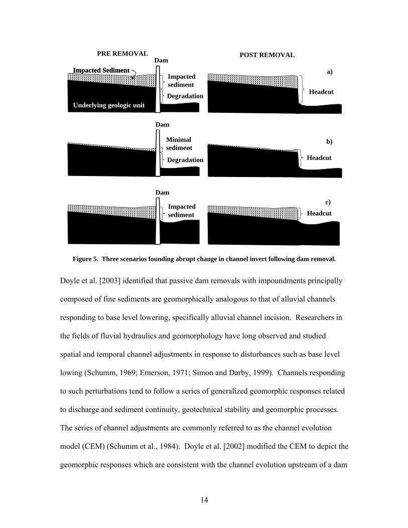
channelization initiated by headcut migration. Headcuts are initiated from an abrupt

change in channel invert caused by either aggradation within the impoundment,

illustrated in Figure 5c, degradation below the dam (Figure 5b), or a combination of the

two (Figure 5a).

14

Degradation Headcut

Degradation

Minimal sediment

Headcut

Dam

Impacted sediment Headcut

Dam

PRE REMOVAL POST REMOVAL

Underlying geologic unit

Impacted SedimentImpacted SedimentDam

Impacted sediment

a)

b)

c)

Figure 5. Three scenarios founding abrupt change in channel invert following dam removal.

Doyle et al. [2003] identified that passive dam removals with impoundments principally

composed of fine sediments are geomorphically analogous to that of alluvial channels

responding to base level lowering, specifically alluvial channel incision. Researchers in

the fields of fluvial hydraulics and geomorphology have long observed and studied

spatial and temporal channel adjustments in response to disturbances such as base level

lowing (Schumm, 1969; Emerson, 1971; Simon and Darby, 1999). Channels responding

to such perturbations tend to follow a series of generalized geomorphic responses related

to discharge and sediment continuity, geotechnical stability and geomorphic processes.

The series of channel adjustments are commonly referred to as the channel evolution

model (CEM) (Schumm et al., 1984). Doyle et al. [2002] modified the CEM to depict the

geomorphic responses which are consistent with the channel evolution upstream of a dam

15

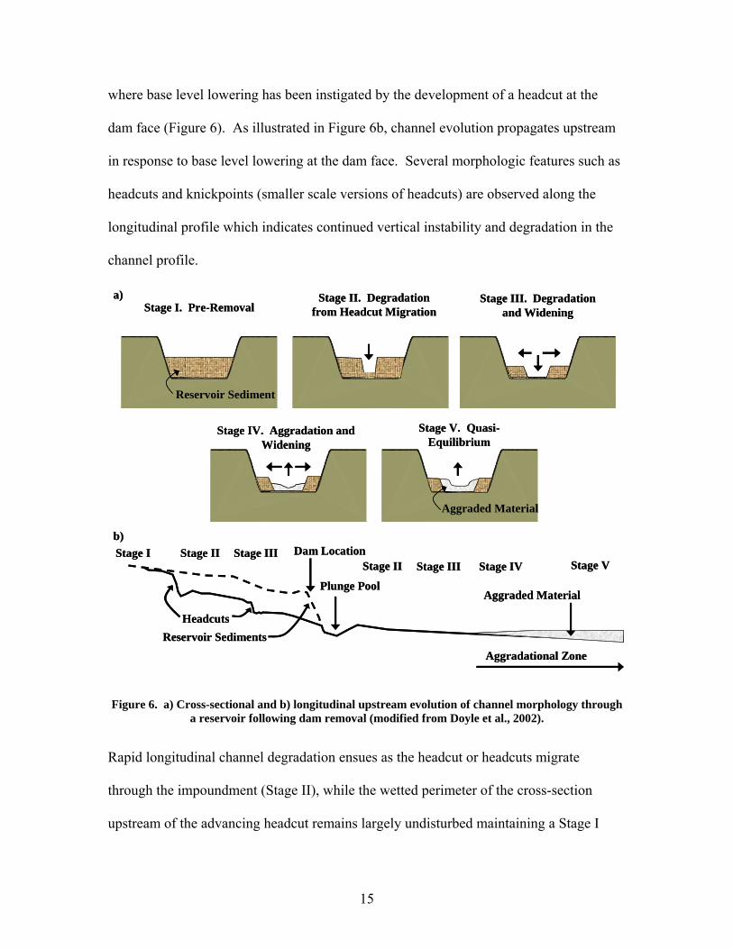
where base level lowering has been instigated by the development of a headcut at the

dam face (Figure 6). As illustrated in Figure 6b, channel evolution propagates upstream

in response to base level lowering at the dam face. Several morphologic features such as

headcuts and knickpoints (smaller scale versions of headcuts) are observed along the

longitudinal profile which indicates continued vertical instability and degradation in the

channel profile.

Stage I. Pre-RemovalStage II. Degradation

from Headcut Migration Stage III. Degradation

and Widening

Stage IV. Aggradation and Widening

Stage V. Quasi-Equilibrium

Reservoir Sediments

Aggraded Material

Dam Location

Plunge Pool

Stage IIStage I

Stage III Stage IV Stage V

Aggradational Zone

Aggraded Material

Reservoir Sediment

Stage II Stage III

Headcuts

a)

b)

Stage I. Pre-RemovalStage II. Degradation

from Headcut Migration Stage III. Degradation

and Widening

Stage IV. Aggradation and Widening

Stage V. Quasi-Equilibrium

Reservoir Sediments

Aggraded Material

Dam Location

Plunge Pool

Stage IIStage I

Stage III Stage IV Stage V

Aggradational Zone

Aggraded Material

Reservoir Sediment

Stage II Stage III

Headcuts

a)

b)

Figure 6. a) Cross-sectional and b) longitudinal upstream evolution of channel morphology through a reservoir following dam removal (modified from Doyle et al., 2002).

Rapid longitudinal channel degradation ensues as the headcut or headcuts migrate

through the impoundment (Stage II), while the wetted perimeter of the cross-section

upstream of the advancing headcut remains largely undisturbed maintaining a Stage I

16

channel morphology (Doyle et al., 2003). The Stage I channel morphology is

characterized by a bankfull channel with an associated floodplain that is commonly either

a riffle-pool or step-pool dominated morphology. Continued channel degradation begins

to decrease the channel gradient (by increasing sinuosity) resulting in increased bank

heights and steeper channel side slopes. This continued geomorphic response leads to

channel widening by mass-wasting and bank failure (Stage III) once bank heights and

angles exceed their critical angles of repose and critical shear stress thresholds (Simon

and Darby, 1999). As channel degradation continues to migrate further upstream, the

reaches closer to the dam face begin to aggrade (Stage IV) resultant from elevated

sediment loads from upstream reaches where Stage III is occurring. The evolution of

Stage V continues to experience aggradation, reductions in channel slope and decreasing

bank height, and channel side slope angles by meander extension (Simon and Darby,

1999). Over time, a new dynamic equilibrium channel and floodplain develops in Stage

V which is similar in cross-sectional profile to Stage I but at a lower base elevation.

The geomorphic response throughout the stages of the CEM is often expressed using

Lane’s stream power proportionality (Lane, 1955):

[ 1 ]

where QF is the channel forming discharge [L3 T-1], So is the bed slope [-], Qs is the bed

material discharge [L3 T-1], di is the characteristic particle size [L], and γW [M L-2T-2] and

γS [M L-2T-2] are the specific weights of water and sediment respectively. The initial

disturbance is caused by the localized increase in bed slope at the headcut causing an

isSoFw dQSQ γγ ∝

17

increase in the sediment discharge and permissible particle size. This describes the

evolution from the first to the second stage of channel evolution. In each subsequent

stage, an imbalance is present causing corresponding shifts in the other variables

expressed in Equation 1. As the channel tends towards a more stable state, such that a

new dynamic equilibrium is attained in Stage V, a new balance is attained in Equation 1

which has adjusted to the surrounding topographic, geologic and hydraulic environment.

Differences exist in the sediment routing and carrying capacity characteristics within

each stage of the channel evolution sequence which is strongly related to bank heights

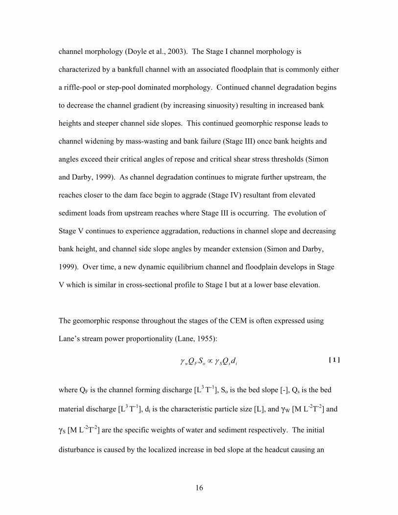
and access to the adjacent floodplain. Flows that frequently overtop their banks onto

floodplains (Stages I and V) maintain lower in-channel velocities and shear stresses

relative to the incised channel reaches where there is limited access to the floodplain

(Stages II, III, IV). Figure 7 illustrates the resulting average velocities for increasing

discharge for the five different stages of channel evolution. In Stage II where vertical

incision occurs, there is limited access to the adjacent floodplain and higher flows are

contained within the limits of the channel. As a result, velocities continue to increase

with increasing discharge. In Stages III and IV where channel widening ensues, the

range in discharge may still be contained within the channel cross-section with no access

to the floodplain; however, with the increasing cross-sectional area, velocities begin to

decrease relative to Stage II. Points of inflection in Stages I, IV and V indicate flow

conditions where floodplain access is achieved. A similar response is observed for

average channel shear stress whereby the hydraulic radius increases more dramatically in

Stages II, III and IV relative to Stages I and V. In the stages of channel evolution where

velocities and shear stresses increase, there is an increased tendency for channel

18

degradation to occur for the reason that velocity and shear stress thresholds may be

exceeded relative to the bed material sizes and cohesiveness required to maintain channel

bed and bank stability.

DISCHARGE (m3/s)

AV

ER

AG

E C

HA

NN

EL

VE

LOC

ITY

(m/s

)

STAGE II

STAGE III

STAGE IV

STAGE I & V

QBF Q

2

Q20

Q50

Q10

0

Figure 7. Average channel velocity profiles for increasing discharge within each stage of the channel evolution model suggested by Doyle et al., 2002. QBF, Q2, Q20, Q50, Q100 values represent the bankfull,

2-year, 20-year, 50-year, and 100-year discharge frequency magnitudes respectively.

Inherent within Figure 7 is the observation that where inflections occur in the velocity

profiles (and in the corresponding shear stress profiles), there are particular discharges

that dominate the rate of channel evolution known as the channel forming discharge (QF).

The channel forming discharge is defined as the theoretical discharge, if maintained

indefinitely, that would produce the same channel geometry as the natural long-term

hydrograph (Copeland et al., 2000). This discharge is significant as many researchers

and practitioners use this single representative discharge to determine the stable channel

19

geometry (Copeland et al., 2000). In channel Stages I and V, bankfull discharge (QBF)

[L3 T-1] dominates the channel evolution which is defined as the discharge, over a long

period of time that defines the dynamically-stable equilibrium channel (Leopold et al.,

1964). In floodplain dominated stream morphologies, this stage is commensurate with

the top of the bank just prior to flows entering the flood plain, thus QBF = QF. The

recurrence interval or frequency of flows that overtop the banks in the unstable sections

(Stages II – IV) is often much greater than the recurrence interval of bankfull discharge

associated with the stable sections and occurs too infrequently to define the channel form.

In these channel morphologies, effective discharge QEFF [L3 T-1] dominates the evolution

of the channel evolution (i.e. QF = QEFF). Effective discharge is defined as the discharge,

or range of discharges, that transports the largest proportion of annual sediment loads

over the long period of time (Wolman and Miller, 1960). A graphical representation of

the bed material load histogram, as a function of sediment transport and frequency of the

transport used to define effective discharge, after Biedenharn and Copeland [2000], is

illustrated in Figure 8.

20

EFFECTIVE DISCHARGE

DISCHARGE

(I)

FRE

QU

EN

CY

(II)

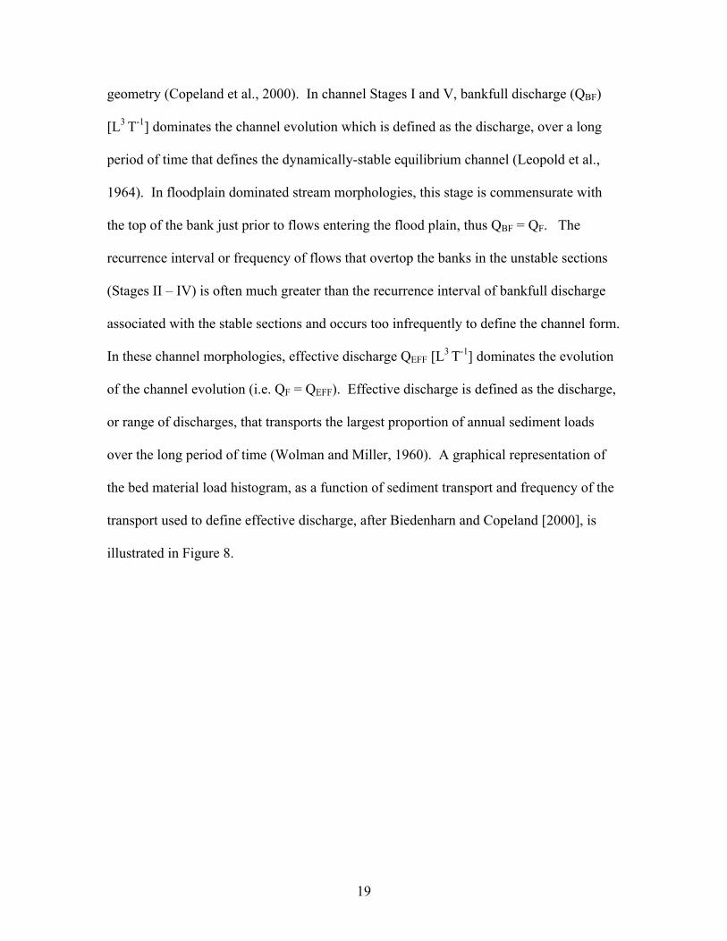
SED

IME

NT

DIS

CH

AR

GE

RA

TIN

G C

UR

VE

(III

)C

OL

LE

CT

IVE

SE

DIM

EN

T D

ISC

HA

RG

E

(I)

(III)(II)

Figure 8. Derivation of total sediment load surcharge curve to predict effective discharge (modified from Biedenharn and Copeland, 2000).

Determining the effective discharge is a theoretical calculation which cannot be field

validated. Effective discharge is typically determined by performing a partial duration

series analysis on a sufficiently long time series (typically greater than 42 years of record)

to determine the flow frequency distribution. After both the partial (pdf) and cumulative

(cdf) distribution frequencies have been determined, the sediment pdf and cdf are

calculated by use of a rating curve typically in the form of:

[ 2 ]

where QSi [M T-1] is the sediment transport rate related to discharge observed (Qi) [L3 T-1]

and a and b are sediment rating curve regression fitting parameters. The sediment pdf is

plotted as a function of discharge, and the local maxima of the resulting histogram is

biSi aQQ =

21

defined as the effective discharge (QEFF) as illustrated in Figure 8. It should be noted that

in channel evolution stages I and V QF = QBF = QEFF.

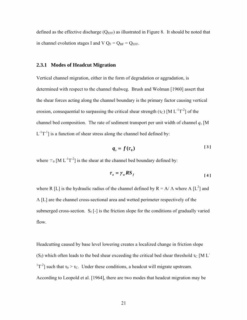
2.3.1 Modes of Headcut Migration

Vertical channel migration, either in the form of degradation or aggradation, is

determined with respect to the channel thalweg. Brush and Wolman [1960] assert that

the shear forces acting along the channel boundary is the primary factor causing vertical

erosion, consequential to surpassing the critical shear strength (τC) [M L-1T-2] of the

channel bed composition. The rate of sediment transport per unit width of channel qs [M

L-1T-1] is a function of shear stress along the channel bed defined by:

[ 3 ]

where t0 [M L-1T-2] is the shear at the channel bed boundary defined by:

[ 4 ]

where R [L] is the hydraulic radius of the channel defined by R = A/ Λ where A [L2] and

Λ [L] are the channel cross-sectional area and wetted perimeter respectively of the

submerged cross-section. Sf [-] is the friction slope for the conditions of gradually varied

flow.

Headcutting caused by base level lowering creates a localized change in friction slope

(Sf) which often leads to the bed shear exceeding the critical bed shear threshold τC [M L-

1T-2] such that τ0 > τC. Under these conditions, a headcut will migrate upstream.

According to Leopold et al. [1964], there are two modes that headcut migration may be

)( 0τfqs =

fwo RSγτ =

22

predisposed to follow: migration of a vertical headcut where the vertical form is

maintained in an upstream propagation; or migration of an initially vertical headcut that

flattens along its migration path until eliminated. Factors that determine the migration

mode are characteristics of the bed material sediments and the hydraulic properties of the

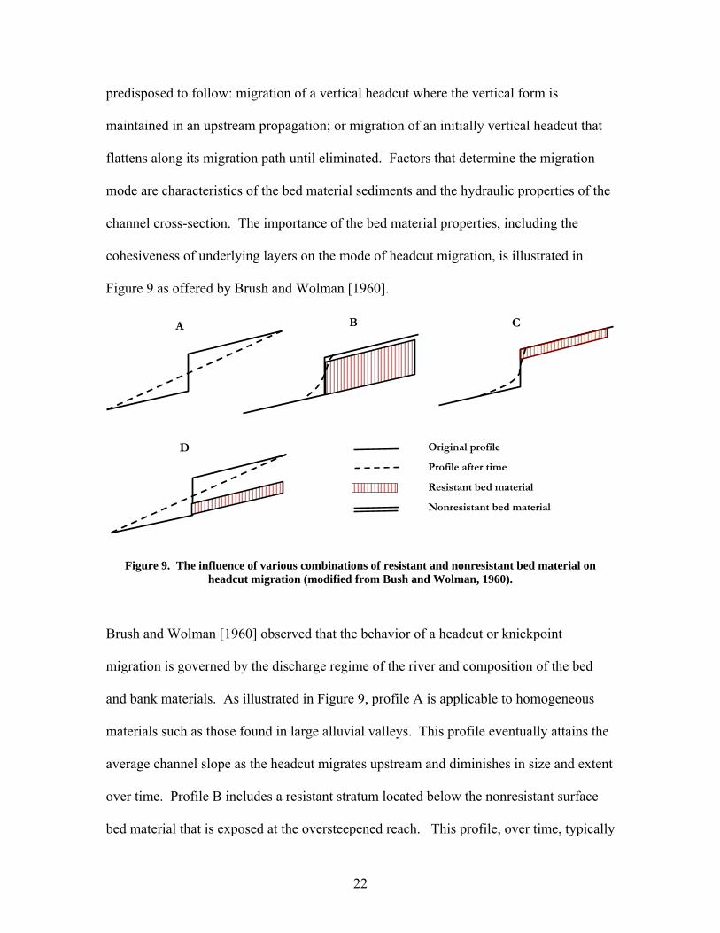
channel cross-section. The importance of the bed material properties, including the

cohesiveness of underlying layers on the mode of headcut migration, is illustrated in

Figure 9 as offered by Brush and Wolman [1960].

Original profile

Profile after time

Resistant bed material

Nonresistant bed material

A B C

D

Figure 9. The influence of various combinations of resistant and nonresistant bed material on headcut migration (modified from Bush and Wolman, 1960).

Brush and Wolman [1960] observed that the behavior of a headcut or knickpoint

migration is governed by the discharge regime of the river and composition of the bed

and bank materials. As illustrated in Figure 9, profile A is applicable to homogeneous

materials such as those found in large alluvial valleys. This profile eventually attains the

average channel slope as the headcut migrates upstream and diminishes in size and extent

over time. Profile B includes a resistant stratum located below the nonresistant surface

bed material that is exposed at the oversteepened reach. This profile, over time, typically

23

maintains a headcut or knickpoint profile and has a relatively slow rate of upstream

channel retreat. Profile C, is similar to that of profile B with the exception that the

upstream resistant bed material overlies a more erodible underlying unit. Similar to

profile B, the headcut shape of profile C remains relatively intact. The rate of upstream

channel migration of profile C is dependent upon the rate of erosion of the underlying

upstream layer, related to toe scour, causing the overriding layer to cantilever and fail.

Lastly, profile D is a variant of the three preceding profiles. The channel response may

behave similar to that of profile A if the resistant layer is located below the vertical centre

of the over-steepened reach and the resulting channel bed slope is sufficiently shallow

such that τ0 < τC. Conversely, if the resistant layer is positioned above the centre of the

over-steepened reach, the profile of the headcut and the localized channel bed slope may

remain and continue to migrate upstream if the localized friction slope remains

sufficiently large such that τ0 > τC along the channel thalweg.

Begin et al. [1980] numerically evaluated upstream headcut migration for the two general

profiles of sustained headcut migration and flattening with upstream channel distance.

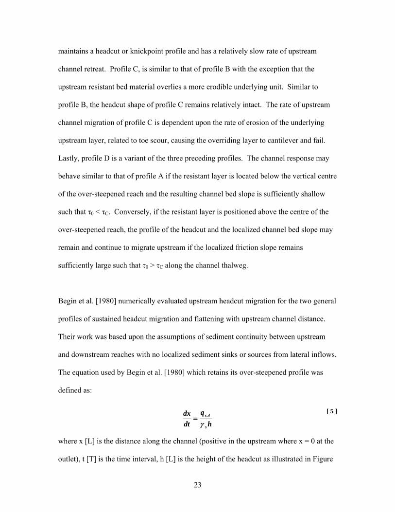
Their work was based upon the assumptions of sediment continuity between upstream

and downstream reaches with no localized sediment sinks or sources from lateral inflows.

The equation used by Begin et al. [1980] which retains its over-steepened profile was

defined as:

[ 5 ]

where x [L] is the distance along the channel (positive in the upstream where x = 0 at the

outlet), t [T] is the time interval, h [L] is the height of the headcut as illustrated in Figure

hq

dtdx

s

ds

γ=

24

10, qSd and qSU are the unit sediment discharges of the downstream and upstream reaches

respectively relative to the location of the headcut where qS and γS have been previously

defined.

α

h

Bed at t1

Bed at t2

x1

x2

qsd

qsu

Figure 10. The physical parameterization of a of a headcut profile (modified from Begin et al., 1980).

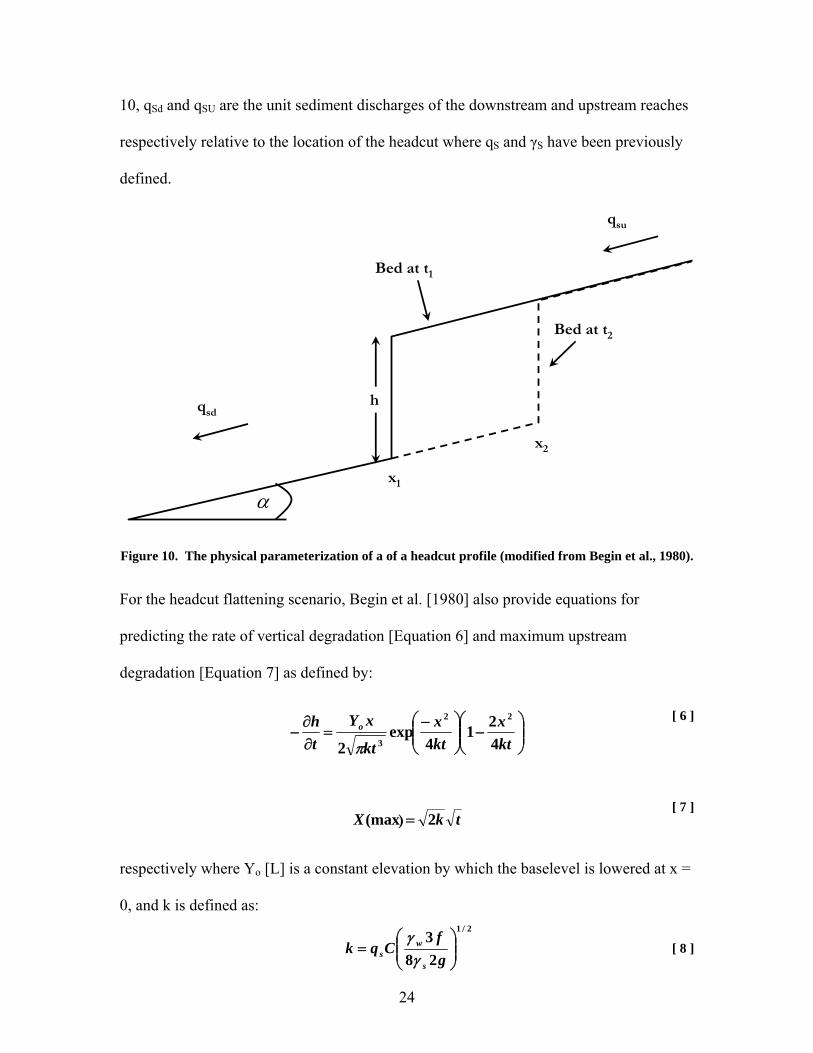
For the headcut flattening scenario, Begin et al. [1980] also provide equations for

predicting the rate of vertical degradation [Equation 6] and maximum upstream

degradation [Equation 7] as defined by:

[ 6 ]

[ 7 ]

respectively where Yo [L] is a constant elevation by which the baselevel is lowered at x =

0, and k is defined as:

[ 8 ]

⎟⎟⎠

⎞⎜⎜⎝

⎛−⎟⎟

⎠

⎞⎜⎜⎝

⎛ −=

∂∂

−ktx

ktx

kt

xYth o

421

4exp

2

22

3π

2/1

283

⎟⎟⎠

⎞⎜⎜⎝

⎛=

gf

Cqks

ws γ

γ

tkX 2(max )=

25

where f [-] is the Darcy-Weisbach friction factor, g [L T-2] is the acceleration due to

gravity, and C [-] is the coefficient of friction, and all other terms have been previously

been defined.

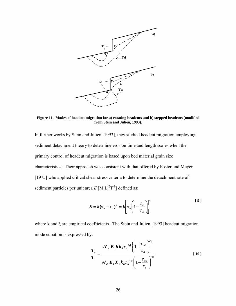
Stein and Julien [1993] studied the migration of headcuts similar to those considered by

Begin et al. [1980]; however, in this study they considered stepped headcuts that retain

their vertical faces or rotating headcuts that flatten along migration They characterized

the type of headcut, based upon the relative erosion rates in the accelerated region at the

face of the headcut and along the impingement region (defined as the effected reaches

both immediately upstream and downstream of the headcut). They defined TU [T] as the

time for upstream vertical scour to reach the toe of the vertical face of the headcut, as

illustrated in Figure 15, and Td [T] as the downstream timescale for the impingement

scour to develop horizontally and reach the toe of the vertical face of the headcut.

Further, Stein and Julien [1993] defined that the headcuts are maintained if TU > Td, and

rotating headcuts when Td < TU.

26

Td

Tu

Td

Tu

a)

b)

Figure 11. Modes of headcut migration for a) rotating headcuts and b) stepped headcuts (modified from Stein and Julien, 1993).

In further works by Stein and Julien [1993], they studied headcut migration employing

sediment detachment theory to determine erosion time and length scales when the

primary control of headcut migration is based upon bed material grain size

characteristics. Their approach was consistent with that offered by Foster and Meyer

[1975] who applied critical shear stress criteria to determine the detachment rate of

sediment particles per unit area E [M L-2T-1] defined as:

[ 9 ]

where k and ξ are empirical coefficients. The Stein and Julien [1993] headcut migration

mode equation is expressed by:

[ 10 ]

ε

ε

ττ

τττ⎥⎥⎦

⎤

⎢⎢⎣

⎡⎟⎟⎠

⎞⎜⎜⎝

⎛−=−=

o

coco kkE 1)(

uu

dd

u

cuuundd

d

cddduu

d

u

kXBA

khBA

TT

εε

εε

ττ

τ

ττ

τ

⎟⎟⎠

⎞⎜⎜⎝

⎛−

⎟⎟⎠

⎞⎜⎜⎝

⎛−

=

1'

1'

27

where subscripts u and d denote upstream and downstream reaches relative to the

location of the headcut, A’ is an empirical coefficient, and B [M L-3] is soil bulk density.

Stein and Julien [1993] identified that if the ratio of Tu / Td > 1, downstream erosion is

dominant over upstream erosion and a headcut retreat will maintain its vertical form.

Where Tu / Td < 1, a headcut was found to rotate and diminish in form with upstream

propagation.

2.3.2 Lateral Migration of Channels Following Dam Removal

MacBroom [2005] asserts that at sites where low head dams have been removed, channel

degradation occurs primarily in the early stages of evolution by rapid vertical incision

(Stage II of the revised channel evolution model offered by Doyle et al. [2002]), which

creates a steep slope (relative to the surrounding valley slope), low sinuosity stream

channel. In subsequent stages of channel evolution over time, the channel adjusts its

pattern laterally to fit its flow, particle sizes and gradation, and slope; consistent with

Stages III - V of the revised channel evolution model offered by Doyle et al. [2002].

Channel migration is often detrimental to various types of floodplain land-use (Shields et

al., 2000). Lateral adjustment of a channel upstream of a former dam are consistent with

Stages III - V of the revised channel evolution model offered by Doyle et al. [2002]

whereby the subsequent increase in migration rate decreases channel slope and decreases

the cross-sectional area of the effective discharge channel which is tending towards a

state of dynamic equilibrium between discharge continuity, sediment continuity and

slope. Channel widening and migration, by mass-wasting, occurs once bank heights and

28

angles exceed the critical shear strength threshold of the bank material (Simon and

Darby, 1999), also commonly referred to as basal end-point control.

Sheilds et al. [2000] defines the rate of channel movement (or channel activity) as:

[ 11 ]

where channel activity [L T-1] is the mean rate of lateral migration along a river reach as

illustrated in Figure 12 where the channel centrelines at times t1 and t2 are the temporal

changes in channel location.

Rates of channel activity have been empirically and analytically related to combinations

of channel geometry, principally relating mean bend radius of curvature (Rc) [L],

normalized by the mean channel width (W) [L], to migration rates (Hickin and Nanson,

1975; Julien, 2002). Findings show that the greatest rates of channel migration occur

when 2≤ Rc/W ≥ 3, and decrease as Rc/W > 3.

Centreline at time t1

Centreline at time t2

Figure 12. Channel centreline migration over time to define channel activity (modified from Shields et al., 2000).

))( 121 ttt of(Length

Area) (Shaded Activity Channel

−=

29

Although general agreements have been found between RC / W and the rates of channel

migration which relate to the intensity of secondary flow in bends and basal end-point

control, Shields et al. [2000] assert that the nature of the heterogeneity in boundary

materials and channel geometry fail to explain the large variation in migration rates,

especially over shorter time periods. Nanson and Hickin [1983] suggests that the lateral

upstream river adjustments following dam removal are defined by the basal sediment size

and stream power P [M L1T-1] as defined by:

[ 12 ]

where Q is the range in discharges above the low flow conditions where sediment

transport and the ensuing mass wasting processes dominate channel evolution and basal

sediment size. Beatty [1984] further subscribes that mass wasting typically generates

much of the lateral adjustments within an impoundment, a condition which is typified by

great uncertainty and unpredictability in migration rates.

2.4 Sediment Transport and Tractive Force Analysis

Leopold et al. [1964] states that any mechanical system having no mean acceleration

must obtain an equilibrium of applied forces. In the case of solids immersed in fluids, the

excess weight of the solids must be transmitted to the ground either by direct contact, flux

of fluid momentum, or a combination of both. Incipient motion of a single particle is

defined as the threshold conditions between erosion and sedimentation. Moreover,

Papanicolaou [2002] defines the critical condition just less than that necessary to initiate

sediment movement as the threshold, and incipient motion as the commencement of

movement of bed particles that previously were at rest instigated by changing flow

fwQSP γ=

30

conditions. At incipient motion, the coefficient of friction is defined as ratio of forces

FN/FO = 1 as illustrated in Figure 13:

FO

FN=Mg cosb

b

b

Figure 13. Relation of applied and resisting forces on a particle resting on a supporting surface

(modified from Leopold et al., 1964).

where FO [M LT-2] is defined as the frictional stress opposing motion of a particle, and FN

[M LT-2] is the force normal to the bed slope for a simple two-dimensional particle.

Fluid flow around sediment particles exert forces which initiate particle motion and are

resisted by the particle weight and shape (Julien, 1995). Motion of a particle along the

channel bed is initiated when the hydrodynamic moment of forces acting on a particle

causing boundary shear (τo) exceeds the resisting moment shear maximum (τc). As the

slope of the supporting surface increases, as is the case along the bed of a headcut, the

frictional force opposing motion must increase at a rate proportional to cosβ, thus the

resisting force decreases and channel erosion ensues.

The Shields parameter (τ*) is a dimensionless shear stress which compares experimental

results of particle movement thresholds to predict incipient motion, as defined by:

[ 13 ]

sms

m

sms

o

du

d )()(

2*

* γγρ

γγτ

τ−

=−

=

31

where u* [L T-1] is the shear velocity, ds [L] is the representative particle size diameter,

and ρm [M L-3]is the density of the fluid. The Shields method [1936] defines the ratio of

the hydrodynamic forces to the submerged weights when the moment arms are

equivalent. The Shields curve has replicate parameters on both sides of the equation, thus

requiring an iterative approach for a solution (Marsh, 2004). Furthermore, Shields [1936]

determined the critical shear stress corresponding to the beginning of motion (τo = τc) for

a range of particle sizes depending upon whether the encompassing flow condition is

either laminar or turbulent as illustrated in Figure 14:

1 10 102 10310-2

10-1

1

Hydraulically

smoothTransition Hydraulically rough

Motion

No motion

Sand Gravel

( ) 3/1

250*1

⎥⎦

⎤⎢⎣

⎡ −=

mvgGdd

c*τ

Figure 14. Shields particle motion diagram (modified from Julien, 1995).

where the critical values (t*C) of the Shields parameter are approximated as:

32

[ 14 ]

where d* is the dimensionless particle diameter defined as:

[ 15 ]

and vm [L/T] is the kinematic viscosity of fluid, G [-] is the specific gravity of the bed

material, and Ø is the critical angle of repose [-] of the bed material of interest.

Figure 14 can be summarized into a tabular format consistent with that outlined in Table

1 for bed material sizes (ds) and approximate threshold conditions for granular particles at

200C.

50tan6.050tan013.0

193.0tan25.0

3.0tan5.0

**

*4.0

**

*6.0

**

**

>=

<<=

<<=

<=−

ddd

dd

d

c

c

c

c

;

19 ;

;

;

φτφτ

φτ

φτ

( ) 3/1

2*1

⎥⎦

⎤⎢⎣

⎡ −=

mvgGdsd

33

Table 1. Approximate threshold conditions for granular material by particle size (modified from Julien, 1995)

Class name ds (mm) d * Ф (deg) τ*c τc (Pa) u*c (m/s)BoulderVery large >2048 51800 42 0.054 1790 1.33Large >1024 25900 42 0.054 895 0.94Medium >512 12950 42 0.054 447 0.67Small >256 6475 42 0.054 223 0.47CobbleLarge >128 3235 42 0.054 111 0.33Small >64 1620 41 0.052 53 0.23

GravelVery coarse >32 810 40 0.05 26 0.16Coarse >16 404 38 0.047 12 0.11Medium >8 202 36 0.044 5.7 0.074Fine >4 101 35 0.042 2.71 0.052Very fine >2 50 33 0.039 1.26 0.036SandVery coarse >1 25 32 0.029 0.47 0.0216Coarse >0.5 12.5 31 0.033 0.27 0.0164Medium >0.25 6.3 30 0.048 0.194 0.0139Fine >0.125 3.2 30 0.072 0.145 0.0120Very fine >0.0625 1.6 30 0.109 0.110 0.0105SiltCoarse >0.031 0.8 30 0.083 0.083 0.0091Medium >0.016 0.4 30 0.065 0.065 0.0080

In describing the particle size distribution of bed material composed of nonuniform-

noncohesive sediment mixtures, Julien [1995] describes the relationships between critical

particle size movement and the heterogeneity of the bed material surface as illustrated in

Figure 15. The first grain size mixture presented in Figure 15a (No Motion) illustrates

the applied shear stress is unable to move any of the particles and is composed of the

original bed material. In the second scenario (Figure 15b) the shear is increased

triggering motion of the finer particles. As a result of transporting only the finer material,

the remaining surface forms an amour layer which is coarser than the original d50 bed

material and in turn shields the finer underlying particles from erosion. This is the

condition whereby a headcut retreats upstream at a slow rate such that τ0< τC for di<d50.

34

The final case presented in Figure 15c illustrates the condition where sufficient bed shear

exists to initiate movement of all bed material particle sizes. The amour layer is no

longer maintained in this scenario and the displacement of the finer particles to the

surface creates a plane in which the coarse particles can easily roll. This is the condition

when a headcut retreats at the fastest rate upstream, when Sf is sufficiently large such that

τ0> τC for all bed material sizes and gradations.

Motion MotionMotionNo Motion No Motion No Motiontc tc tc

a) No Motion b) Partial Motion c) Full Motion Figure 15. Bed surface for nonuniform grain size mixtures (modified from Julien, 1995).

The critical value of shear stress (τC) for different grain sizes has been related to the 50th

percentile (d50) based upon a bed material grain size analysis (Egiazaroff, 1965; Parker et

al., 1982; Komar, 1987; Ashworth and Ferguson, 1989; Kuhnle, 1992; Wilcock and

Southard, 1997) which is commonly expressed as:

[ 16 ]

where τ*Ci, is the critical shear stress threshold of the bed material particle diameter di and

τ*C50 is the critical shear stress threshold value of the d50 bed material diameter

respectively. Furthermore, z is referred to as a hiding function, which varies widely

)/(/ 5050** ddz icci =ττ

35

(Shvidchenko et al., 2001) and is largely related to particle shape and grain size

gradation. Typical ranges in hiding functions are outlined in Figure 16.

0.01

1

1 Egiazaroff (1965)

2 Parker et al. (1982)

3 Komar (1987)

4 Ashworth and Ferguson (1989)

5 Kuhnle (1992)

6 Wilcock and Southard (1997)

10

100

0.10.1 1 100

50** / cic ττ

50/ ddi

6

3

345

2 1

0.01

1

1 Egiazaroff (1965)

2 Parker et al. (1982)

3 Komar (1987)

4 Ashworth and Ferguson (1989)

5 Kuhnle (1992)

6 Wilcock and Southard (1997)

10

100

0.10.1 1 100

50** / cic ττ

50/ ddi

6

3

345

2 1

Figure 16. Comparison of different hiding functions (modified from Shvidchenko et al., 2001).

2.5 Longitudinal Hydraulic and Sedimentological Channel Evolution Responses to Passive Dam Removal

With both the theory and physical conceptualizations of how channel degradation may

occur upstream of a dam (Sections 2.3 and 2.4), the channel evolution model proposed by

Doyle et al. [2002] (Figure 6) can be interpreted throughout the longitudinal profile of a

river channel. A conceptually based HEC-RAS© model was developed with channel

geometry consistent with Figure 6 to elucidate the hydraulic and sedimentological

processes occurring throughout a river channel upstream of a dam consistent with a

passive restoration recovery approach.

36

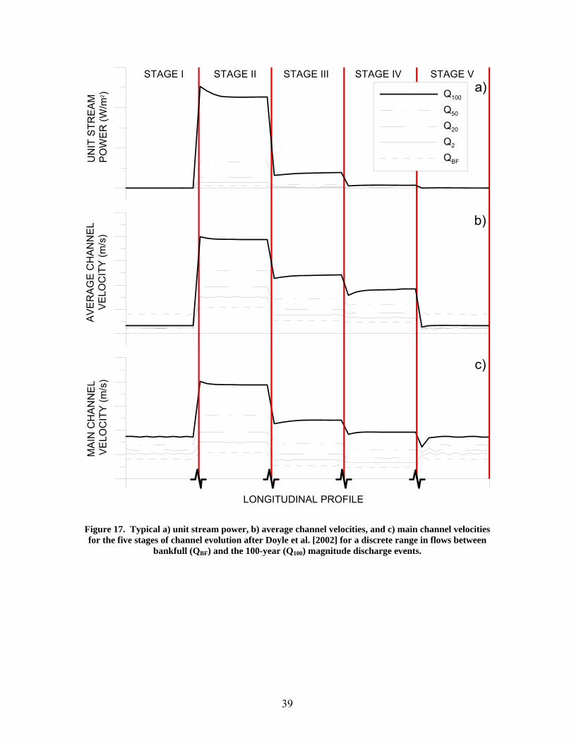
Figure 17 and Figure 18 illustrate the unit stream power ( P ) [M T-1] as defined by:

[ 17 ]

where T [L] is the top width of the channel, the average channel velocity (V ) [L T-1], the

main channel velocity (VMAIN) [L T-1], the average channel shear (τO), and the main

channel shear (τOMAIN). In Stages I and V of the channel evolution sequence, the VMAIN

and τO MAIN are consistent with the bankfull channel hydraulic geometry. Five discrete

flows are illustrated in each CEM stage ranging between bankfull discharge (QBF) and the

100-year return period (Q100).

Figure 17a illustrates that the lowest unit stream power occurs in Stages I and V where

bankfull discharge dominates the flow regime. These are the regions where the channel

is considered to be in a state of quasi-equilibrium. It should also be noted that when the

discharge state exceeds bankfull, the top width of the channel dramatically increases

across the floodplain, thereby maintaining a low unit stream power and a low potential

for channel degradation to occur. Stage II has the highest unit stream power for each

discharge value, which also relates to the channels evolutionary stage where there is no or

limited floodplain relief. The newly formed channel has yet to widen and contains all

discharges within the same channel width. This is also the stage where the highest rates

of vertical erosion occur. The unit stream power in Stages III and IV consistently

decrease as channel widening begins to occur through meander extension. By stage IV

the stream power is sufficiently low such that bed material deposition begins to occur

with the continued decrease in unit stream power.

TQS

P fwγ=ˆ

37

The average channel velocity and main channel velocity have similar responses to those

of the unit stream power for the different discharges, as illustrated in Figure 17b and

Figure 17c respectively. For Stages II – IV, the main channel velocities may be

sufficiently large, such that they exceed the critical particle size thresholds (dC) and the

volumes of bed material transport in these reaches exceeds the flux entering the reservoir

system from upstream. Consequently, with a discrepancy in sediment continuity, channel

degradation ensues. It is also noteworthy to identify that the average bankfull channel

discharge results in the highest average channel velocity (Figure 17b) in Stages I and V

although the main channel discharge (Figure 17c) continues to increase with increasing

discharge. This is common within a floodplain dominated channel morphology and also

typifies the channel morphology where bankfull discharge and effective discharge are

synonymous with the channel forming flow (i.e. QF = QBF = QEFF). In evolution Stages II

– IV where the flow depth and velocities continue to increase with increasing discharge,

there exists the ability to transport greater volumes of sediment. These are the stages

where effective discharge dominates the channel evolution (i.e. QF = QEFF).

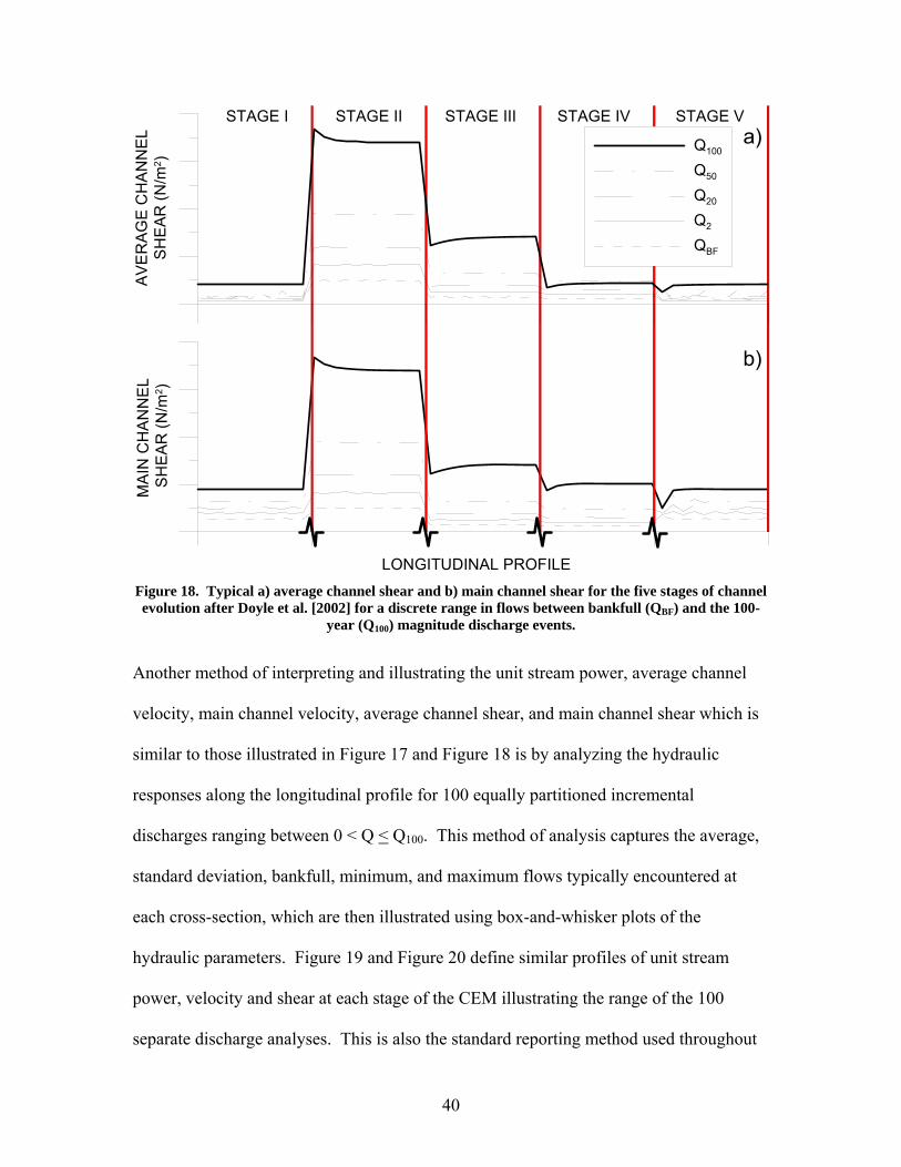
The average channel shear and main channel shear also have similar responses to that of

the unit stream power, average channel velocity and main channel velocity for the

different discharges as illustrated in Figure 18a and Figure 18b respectively. When

discharges exceed the bankfull depths in Stages I and V, the wetted perimeter

significantly increases as the flows begin to inundate their respective floodplains. With

the significant increases in wetted perimeters (Λ) the hydraulic radii (R) begin to

decrease with increasing stage above bankfull depth resulting in the shear stress

38

remaining relatively low in Stages I and V. Conversely, in Stages II – IV with increasing

discharge, there is no or limited access to floodplains. As a result, in Stages II – IV, the

flow depth continues to increase with increasing discharge and the wetted perimeter does

not increase as quickly, relative to Stages I and V, resulting in increased shear stress. The

highest rates of channel shear which occur in Stage II diminish as the evolutionary

sequence tends towards stage IV where sediment deposition may begin to dominate the

evolution of the channel morphology.

39

MA

IN C

HA

NN

EL

VE

LOC

ITY

(m/s

)

LONGITUDINAL PROFILE

STAGE I STAGE II STAGE III STAGE IV STAGE VA

VE

RA

GE

CH

AN

NE

LV

ELO

CIT

Y (m

/s)

UN

IT S

TRE

AM

P

OW

ER

(W/m

2 ) Q100

Q50

Q20

Q2

QBF

a)

b)

c)

Figure 17. Typical a) unit stream power, b) average channel velocities, and c) main channel velocities for the five stages of channel evolution after Doyle et al. [2002] for a discrete range in flows between

bankfull (QBF) and the 100-year (Q100) magnitude discharge events.

40

MA

IN C

HA

NN

EL

SH

EA

R (N

/m2 )

LONGITUDINAL PROFILE

STAGE I STAGE II STAGE III STAGE IV STAGE VA

VE

RA

GE

CH

AN

NE

LS

HE

AR

(N/m

2 )Q100

Q50

Q20

Q2

QBF

a)

b)

Figure 18. Typical a) average channel shear and b) main channel shear for the five stages of channel evolution after Doyle et al. [2002] for a discrete range in flows between bankfull (QBF) and the 100-

year (Q100) magnitude discharge events.

Another method of interpreting and illustrating the unit stream power, average channel

velocity, main channel velocity, average channel shear, and main channel shear which is

similar to those illustrated in Figure 17 and Figure 18 is by analyzing the hydraulic

responses along the longitudinal profile for 100 equally partitioned incremental

discharges ranging between 0 < Q < Q100. This method of analysis captures the average,

standard deviation, bankfull, minimum, and maximum flows typically encountered at

each cross-section, which are then illustrated using box-and-whisker plots of the

hydraulic parameters. Figure 19 and Figure 20 define similar profiles of unit stream

power, velocity and shear at each stage of the CEM illustrating the range of the 100

separate discharge analyses. This is also the standard reporting method used throughout

41

the remainder of this research to present the hydraulic results over the range of discharges

from 0 < Q < Q100.

The analyses based upon this method further illustrate that in Stages I and V, the bankfull

average channel velocity remains the highest (Figure 19b) for the entire range in

discharges considered whereas the unit stream power (Figure 19a), main channel velocity

(Figure 19c), average shear stress (Figure 20a), and main channel shear associated with

bankfull discharge (Figure 20b) are either the lowest or close to the lowest values for the

range in discharges. The small range in standard deviations of the hydraulic parameters

in Stages I and V also addresses the damping effects of the floodplain on hydraulic

responses in these channel morphologies. The smaller total and standard deviation

ranges in hydraulic parameters of Stages I and V identify that there will not be as

dramatic of a response in the channel evolution for the entire range in flows; relative to

Stages II - IV. The greater range in standard deviations and total ranges of the hydraulic

parameters in Stages II – IV indicate a larger vulnerability to channel degradation based

upon the magnitude and recurrence interval of particular discharge events of interest. At

some location within the standard deviation ranges of hydraulic parameters in Stages II –

IV is the discharge associated with the effective discharge that dictates channel evolution.

It is also noted in Stages II – IV that hydraulic conditions associated with bankfull

discharge are notably below each standard deviation, further indicating that QBF is not a

significant discharge of the channel evolution in these stages.

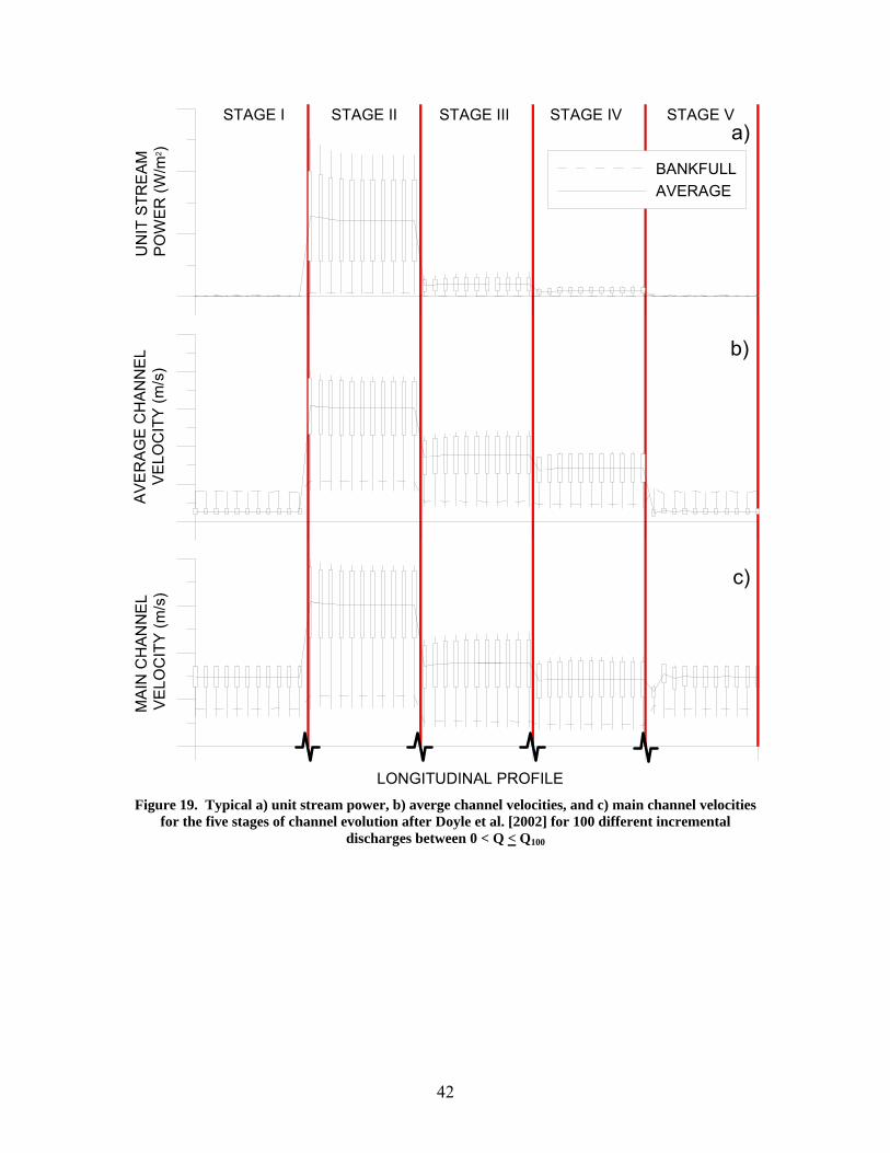
42

MA

IN C

HA

NN

EL

VE

LOC

ITY

(m/s

)

LONGITUDINAL PROFILE

STAGE I STAGE II STAGE III STAGE IV STAGE VA

VE

RA

GE

CH

AN

NE

LV

ELO

CIT

Y (m

/s)

UN

IT S

TRE

AM

P

OW

ER

(W/m

2 )BANKFULLAVERAGE

a)

b)

c)

Figure 19. Typical a) unit stream power, b) averge channel velocities, and c) main channel velocities

for the five stages of channel evolution after Doyle et al. [2002] for 100 different incremental discharges between 0 < Q < Q100

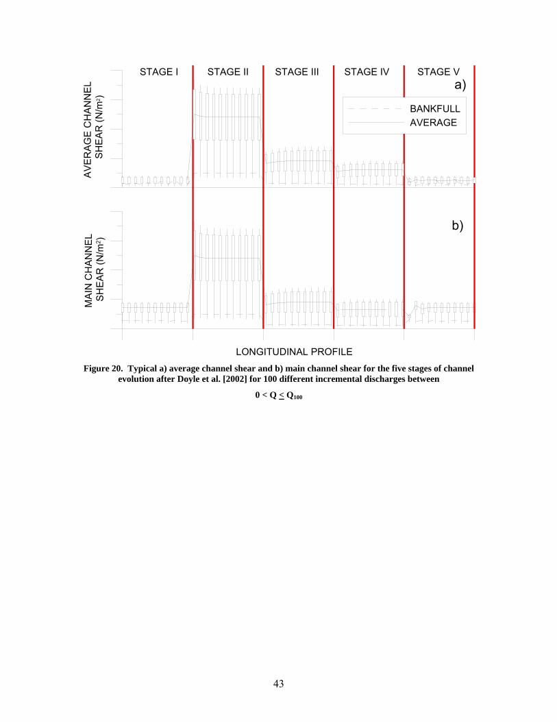
43

MA

IN C

HA

NN

EL

SH

EA

R (N

/m2 )

LONGITUDINAL PROFILE

STAGE I STAGE II STAGE III STAGE IV STAGE VA

VE

RA

GE

CH

AN

NE

L S

HE

AR

(N/m

2 )BANKFULLAVERAGE

a)

b)

Figure 20. Typical a) average channel shear and b) main channel shear for the five stages of channel

evolution after Doyle et al. [2002] for 100 different incremental discharges between

0 < Q < Q100

44

3 FIELD AND ANALYSIS METHODS Upon canvassing local and provincial agencies, 20 decommissioned / failed dams were

identified in Southern Ontario south of the Canadian Shield in glacio-fluvial deposits.

The dams identified had either been removed or failed from severe flooding,

abandonment, or lack of operations maintenance. In order to meet the objectives of this

study no upstream interventions, restorations or rehabilitation could have occurred since

the time of dam failure or removal till present day. The primary selection criteria results

in a morphologic response with minimal anthropogenic disturbances, analogous to the

passive dam remediation approach consistent with an abrupt dam removal and without

any upstream works undertaken. Further, sites were chosen to cover a broad range of

valley slopes and underlying geology (i.e. differing grain sizes) as these are often

principle factors in channel evolution and sediment transport. Based upon the above

criteria, eight dam sites were identified from both aerial and field reconnaissance which

are listed in Table 2 with their associated valley slopes and predominate upstream

catchment area physiography (Chapman and Putnam, 1966). The general locations of the

dams are illustrated in Figure 21. Detailed site locations of each of the dam sites are

outlined in Appendices A – H.

45

Table 2. List of dam study sites, river names, valley slope and dominant upstream physiography.

Ref. No. Dam Name River Name and Neighboring Town

Valley Slope (m/m)

Physiography

1 Croton Dam Big Creek at Delhi 1.80E-03 Sand Plain2 Hawkesville Dam Conestogo River at 1.90E-03 Till Moraine3 Huttonville Dam Credit River at Huttonville 2.70E-03 Till Plain4 Chilligo Dam Ellis Creek at Cambridge 3.10E-03 Spillway5 Greenfield Dam Nith River at Greenfield 1.70E-03 Kame Moraine6 Sutton Dam Patterson Creek at Simcoe 2.05E-03 Sand Plain7 Teeswater Dam Teeswater River at Teeswater 2.40E-03 Kame Moraine8 Bognor Dam Walter's Creek at Bognor 8.00E-03 Drumlinized Till Plain

CANADA

U.S.A.

U.S.A.

Ontario

Quebec

8

7

45

32

1 6

CANADA

U.S.A.

U.S.A.

Ontario

Quebec

8

7

45

32

1 6

Figure 21. Locations of study sites within Southern Ontario.

Background studies were conducted for each site using the Geographic Information

Systems (GIS) program ArcGIS® and AutoCAD®. Time series aerial photographs were

acquired for each site, ranging from 1954 – 2002 photographs provided by the Ontario

department of Lands, Ontario Ministry of Natural Resources and the local conservation

authorities. Hard copy aerial photographs were scanned and georeferenced for time-

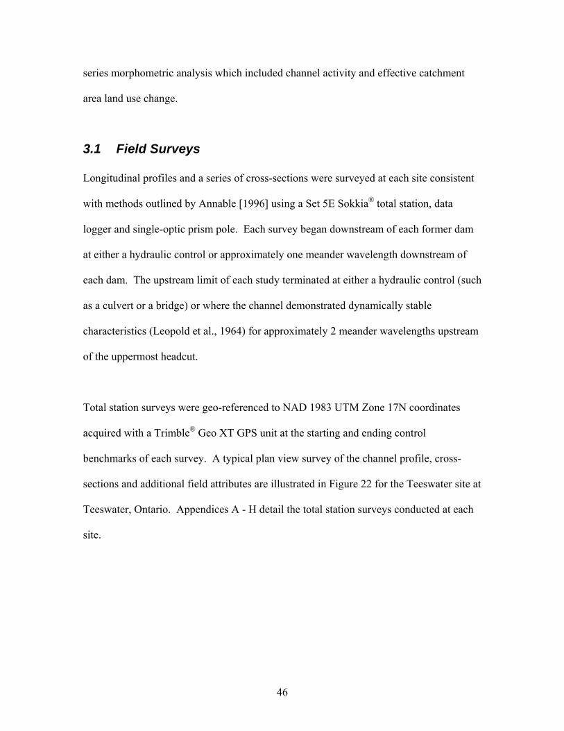
46

series morphometric analysis which included channel activity and effective catchment

area land use change.

3.1 Field Surveys Longitudinal profiles and a series of cross-sections were surveyed at each site consistent

with methods outlined by Annable [1996] using a Set 5E Sokkia® total station, data

logger and single-optic prism pole. Each survey began downstream of each former dam

at either a hydraulic control or approximately one meander wavelength downstream of

each dam. The upstream limit of each study terminated at either a hydraulic control (such

as a culvert or a bridge) or where the channel demonstrated dynamically stable

characteristics (Leopold et al., 1964) for approximately 2 meander wavelengths upstream

of the uppermost headcut.

Total station surveys were geo-referenced to NAD 1983 UTM Zone 17N coordinates

acquired with a Trimble® Geo XT GPS unit at the starting and ending control

benchmarks of each survey. A typical plan view survey of the channel profile, cross-

sections and additional field attributes are illustrated in Figure 22 for the Teeswater site at

Teeswater, Ontario. Appendices A - H detail the total station surveys conducted at each

site.

47

!

!

!

!!

!

!

!

!

! !

!

!

!

!!!

!!!! !! !! !!

!

!

!

!

!

!!

!

!

!

!

!

!

!

!

!

!!

!

!

!

!

!

!

!

!

!

!

!

!

!

!

!

!

!

!

!

!!

!!

! !! !

!

!!!!!!!!

!

!

!!!!!!

!

!

!

!

!

!

!!!!!

!

!!!!!

!

!!

!!!!

!!

!!

!!

!!

!!!!!!!!!!

!!!!

!

!!!!

!

!!!!!!!!!!!!!!!!! !

!!

!!!!!!!!!!

!

!!

!

!!!!!!!!!!!!!!!

!

!!!!!!!!!!!!!!

!

!!!! ! !

! ! ! !!! !!!!!!!!!!!!!!

!!!! !!!!!

! !!! ! !

!!!

!

!

!

!!

!

!

!

!

!

!

!

!

!

!

!

!!!!!

! !

!!

!

!

!

!

!

!!

!

!!!!

!

!!!!!

!!!

!!!

!

!

!

!

!

!

!

!

!

!!

!

!!!!!

!

!!!

!

!

!

!!

!

!

!

!

!

!

!!

!

!!!

!

!! !!

!

!

!!

!!!!

!

!

!

!

!

!

!

!

!

!

!

!

!

!

!

!

!!

!

!

!

!!!

!

!!

!!

!

!!!

!!!

!!! !!!

!

!!!

!

!

!!

!

!!

!

!!

!!

!

!

!!!!!!!!

!!!!

!!!!!!

!

!

!

!

!!!

!

!

!

!

!!!!

!

!!!!!!!!!!

!

!

!

!!

!

!

!!!!!!

!

!

!

!

!

!

!

!

!

!

!

!

!

!

!

!!!!

!

!

!

!

!

!

!!!!!!

!

!!!

!

!

!!!!!!

!

!

!

!

!!!!!!

!!

!!

!

!!!!!!!!

!

!!

!!!!!!!

!

!!

!

!

!

!

!

!!

!!!!!!!!!

!

!!!!

!

!

!

!!

!!!!!

!

!

!

!

!

!!

!

!

!

!

!

!

!!

!!

!!

!

! !!!!!! !

!!!!!!!!!!! !!!!!!!!!

!!!!

!!! !!!!!!!!

!

!!

!!!!!

!!

!

!

!!

!

!!

!

!!

!!!!! !!!!!!!

!!! !

!

!!

!

!!!!!!!!!!

!!!!

!!

!

!

!!

!

!! !!!!!

!!

!!!!!

!!

!

!!

! !

!

!

!

!

!

!!!!!!

!

!

!!

!

!

!!!!!!!

!!

!!

! !!

!!!

!

!

!

!

!!!

!

!!!!!!!!

!!!!!!!!!

!

!!!!!! !

!!!!!!!!!!!!!!

!!

!

!

!

!

!

!

!!! ! ! ! !

!!

!!!!!!

!

!!

!

! !!

! ! !!!!

!!!!!!

!

!

!

!!

!

!

!!!!!!

!

!!!!!!!

!!!!!!!!!!

!!! !! !

!!!!!!! !!!

!

!

!!

!!

! !

!!

!

!

!! !! !! !!!!!!!!!!!!!!!!

!!!

!

!

!

!

!

!

!

!!!!!!!!!!!!!!!!

!

!

!

!

!

!

!

!

!

!

!

!!

!

!

!

!

!

")")")

UPPERMOST HEADCUT

CLIN

TON

COUNTY RD 6

HILLCREST

GORDON

JAMES

MARCY

UNION

CLAR

IND

A

ELIZABETH

ANN

MILL

BRO

WN

LEE

BROWN

ISABELLA

RIVER

VIEW

CLA

RIN

DA

0 10.5 km

­Legend

") Dam Location! Survey Points

Reservoir Area

TEESWATER

FLOW

DAM LOCATION

Figure 22. Example plan view of a field survey of Teeswater River at Teeswater.

3.1.1 Longitudinal Profiles

Thalweg measurements were obtained along the study reach at approximately every

bankfull channel width, in addition to the maximum inverts of pools, notable changes in

channel slope, and at the tops and bottoms of riffles and headcuts respectively consistent

with the methods outlined by Annable [1996]. Using thalweg measurements, a

longitudinal profile was developed for every site as illustrated in Figure 23 for the

Teeswater dam. Appendices A - H also detail each of the longitudinal profiles.

48

0 500 1000 1500 2000LONGITUDINAL DISTANCE (m)

94

96

98

100

102B

ED

ELE

VA

TIO

N (m

)

DA

M

HE

AD

CU

T

RE

SE

RVO

IR E

XTE

NT

HE

AD

CU

T

HE

AD

CU

T

Figure 23. Longitudinal profile of Teeswater River at Teeswater.

The lengths and slopes of riffles, runs, headcuts, knickpoints, inter-riffle and inter-pool

lengths were determined from the longitudinal profile. Slopes and lengths were

determined from the average elevation of the three survey points at the top and bottom of

each morphological feature respectively.

3.1.2 Cross-Sectional Profiles

Cross-sections define the geometric boundary conditions of a river or stream

perpendicular to flow along the channel and adjacent floodplains. Cross-sections were

defined and measured perpendicular to the channel within the upper third of each riffle,

run or headcut and extended out into the floodplains in sufficient detail to define cross-

sections for undertaking hydraulic analysis using Hydrologic Engineering Center’s River

Analysis System (HEC-RAS® 4.0) for flood conditions. At each cross-section,

characteristics such as top and bottom of banks, bankfull stage, and thalweg were

defined, in addition to all notable breaks in slope and terraces identified in the field.

Ideally, the extent of each cross-section was surveyed from, at minimum, the top of

49

valley walls to the channel thalweg. In cases where it was not possible to extend the

survey to the top of the valley walls, due to line of sight limitations with the total station,

the extents of the cross-section along the floodplain were extrapolated using topographic

maps at a scale of 1:10 000 once the field surveys were geo-referenced.

3.1.3 Sediment Sampling Bed material sampling was undertaken to obtain particle size distributions of riffles, runs,

and headcuts within each disturbed reach in addition to reaches upstream of the erosional

effects or the uppermost headcut. Sampling methods were consistent with those offered

by Klingeman and Emmett [1982] and Annable [1996] for the gravel- and cobble-bed

streams; and by Ashmore [1988] for the sand-bed channels. Two-to-three random

locations (dependent on channel width) across both the upper and lower thirds of each

feature were sampled and their locations geographically referenced using a Trimble®

GeoXT. Figure 24 and Figure 25 illustrate the typical locations where samples were

collected along riffles and headcuts respectively.

50

TOP

OF

RIF

FLE

BO

TTO

M

OF

RIF

FLE

CROSS

SEC

TION

VALLEY TREND

FLOW

BANKFULL CHANNEL

BANKFULL CHANNEL

SAMPLE LOCATIONSSAMPLE LOCATIONS

Figure 24. Locations of bed material samples along a riffle.

TOP

OF

HEA

DC

UT

BOTT

OM

OF

HEA

DC

UT

VALLEY TREND

FLOW

SURV

EYED

CRO

SS

SECT

IONS

ABO

VEAN

D BE

LOW

HE

ADCU

T

SAMPLE LOCATIONS SAMPLE LOCATIONS

Figure 25. Locations of bed material samples along a headcut.

51

Notable exceptions to the methods above were in the cases where the bed material was

principally comprised of boulders too large to be extracted for laboratory analysis. In

these cases, a modified version of the Wolman [1954] pebble count method was

employed. The modified Wolman pebble count method consisted of two passes between

the bankfull channel limits along the bed of the channel on the morphological feature of

interest randomly sampling approximately 50 particles. The three principle particle axes

of each particle were measured (a-axis, b-axis, c-axis) which relate to the largest,

intermediate and smallest particle axis lengths respectively, and the particle converted to

its spherical volume equivalent. Using this volume estimate, the mass was estimated

using a bulk density of 2650 kg/m3. Grain size analyses were conducted on each

sediment sample collected using dry sieving methods at 0.5φ intervals (Friedman and

Sanders, 1978) for particles smaller than 32mm (di < 32mm), where

[ 18 ]

Particles greater than 32mm were measured and massed individually in the field and

segregated into 0.5 φ intervals. Both field and dry sieve data on each sample were

combined after the various sampling and particle sorting methods and the d5, d16, d25, d50,

d75, d84, d95 percentiles determined. The mean, standard deviation, kurtosis and skewness

of each sediment sample were also calculated in addition to a composite grain size

distribution (Friedman and Sanders, 1978) of each morphological feature (i.e. riffles,

runs, headcuts, knickpoints). Figure 26 illustrates the analysis results of sediment

sampling of a riffle, along with the respective sampling locations. Appendices A – H

contain these analyses for each site.

).(log 2 id=φ

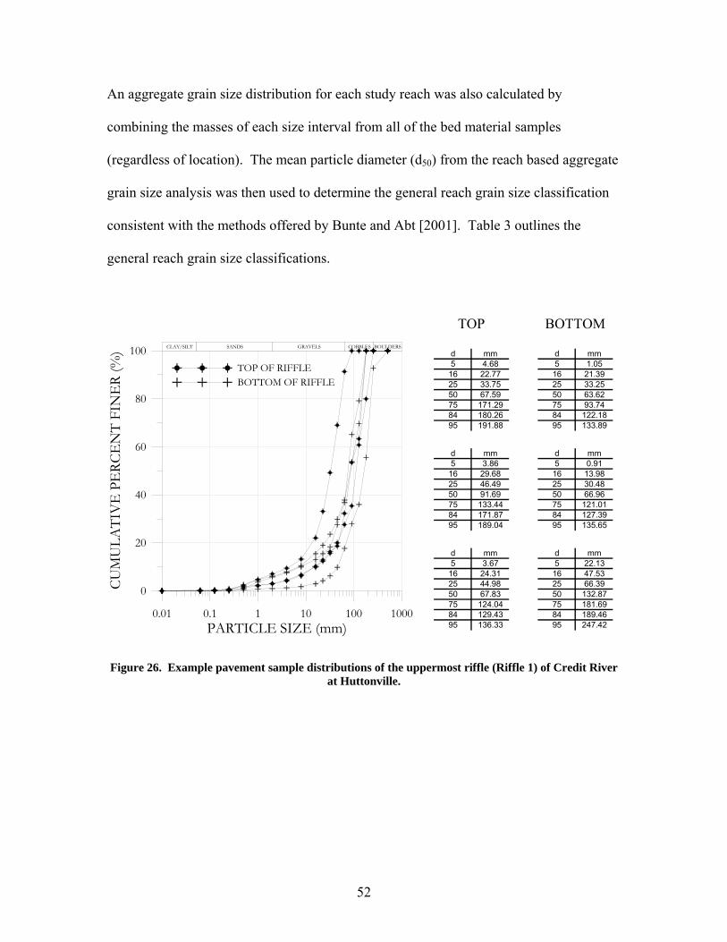
52

An aggregate grain size distribution for each study reach was also calculated by

combining the masses of each size interval from all of the bed material samples

(regardless of location). The mean particle diameter (d50) from the reach based aggregate

grain size analysis was then used to determine the general reach grain size classification

consistent with the methods offered by Bunte and Abt [2001]. Table 3 outlines the

general reach grain size classifications.

TOP

d mm5 4.6816 22.7725 33.7550 67.5975 171.2984 180.2695 191.88

BOTTOM

d mm5 1.0516 21.3925 33.2550 63.6275 93.7484 122.1895 133.89

d mm5 3.8616 29.6825 46.4950 91.6975 133.4484 171.8795 189.04

d mm5 0.9116 13.9825 30.4850 66.9675 121.0184 127.3995 135.65

0.01 0.1 1 10 100 1000PARTICLE SIZE (mm)

0

20

40

60

80

100

CUM

ULA

TIV

E P

ERC

EN

T FI

NE

R (%

)

TOP OF RIFFLEBOTTOM OF RIFFLE

CLAY/SILT SANDS GRAVELS COBBLES BOULDERS

d mm5 3.6716 24.3125 44.9850 67.8375 124.0484 129.4395 136.33

d mm5 22.1316 47.5325 66.3950 132.8775 181.6984 189.4695 247.42

Figure 26. Example pavement sample distributions of the uppermost riffle (Riffle 1) of Credit River at Huttonville.

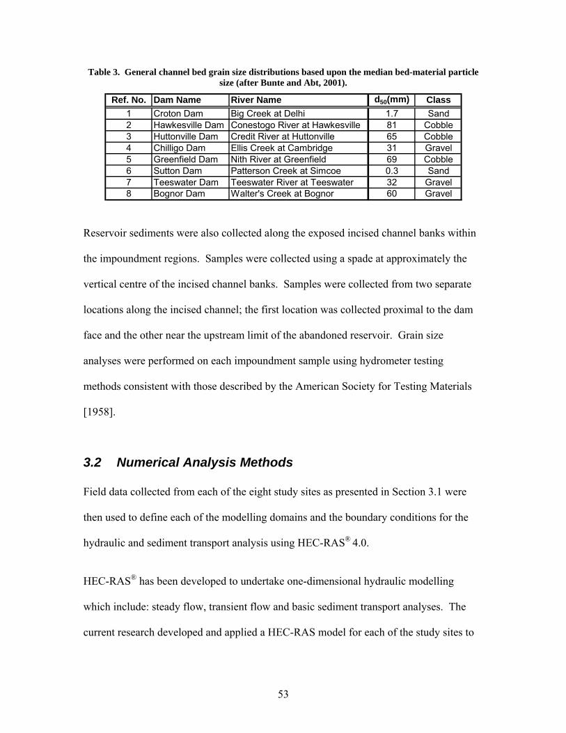
53

Table 3. General channel bed grain size distributions based upon the median bed-material particle size (after Bunte and Abt, 2001).

Ref. No. Dam Name River Name d50(mm) Class1 Croton Dam Big Creek at Delhi 1.7 Sand2 Hawkesville Dam Conestogo River at Hawkesville 81 Cobble3 Huttonville Dam Credit River at Huttonville 65 Cobble4 Chilligo Dam Ellis Creek at Cambridge 31 Gravel5 Greenfield Dam Nith River at Greenfield 69 Cobble6 Sutton Dam Patterson Creek at Simcoe 0.3 Sand7 Teeswater Dam Teeswater River at Teeswater 32 Gravel8 Bognor Dam Walter's Creek at Bognor 60 Gravel

Reservoir sediments were also collected along the exposed incised channel banks within

the impoundment regions. Samples were collected using a spade at approximately the

vertical centre of the incised channel banks. Samples were collected from two separate

locations along the incised channel; the first location was collected proximal to the dam

face and the other near the upstream limit of the abandoned reservoir. Grain size

analyses were performed on each impoundment sample using hydrometer testing

methods consistent with those described by the American Society for Testing Materials

[1958].

3.2 Numerical Analysis Methods Field data collected from each of the eight study sites as presented in Section 3.1 were

then used to define each of the modelling domains and the boundary conditions for the

hydraulic and sediment transport analysis using HEC-RAS® 4.0.

HEC-RAS® has been developed to undertake one-dimensional hydraulic modelling

which include: steady flow, transient flow and basic sediment transport analyses. The

current research developed and applied a HEC-RAS model for each of the study sites to

54

investigate the hydraulic characteristics of the study reaches over a series of discharges

ranging between 0 < Q < Q100.

In the development of each site model, additional cross-sections were required to reduce

conveyance ratio errors. Cross-sections were added at locations where numerical errors

were identified by using the representative cross-sectional form of the adjacent upstream

and downstream cross-sections and adjusting the elevation of the thalweg of the

synthetically generated cross-section to be consistent with the field measured thalweg

elevation.

In some instances, a location of hydraulic control was not identified in the field to

provide downstream boundary conditions. In these situations, a downstream hydraulic

control flow condition was assumed, however, the downstream limit of the site model

was extended downstream such that normal depth was achieved immediately downstream

of the dam for discharge conditions ranging between 0 < Q < Q100. The river reach was

typically extended downstream of the dam a distance equal to 40 times the top width (T)

of the Q100 discharge event. In mild slope channel conditions, the channel extension

distance is considered to be adequate to address any numerical artifacts of assuming a

downstream critical flow depth (Totz and Klotz, 2003). An average channel cross-

section was assumed for the downstream channel extension reach based upon surveyed

cross-sections downstream of each dam. Stream channel slope (SO) was determined from

the relationship:

[ 19 ]

Ω= V

OSS

55

where SV [-] is the valley slope and Ω [-] is the channel sinuosity down stream of the

dams which were determined from 1:10000 topographic maps and / or digital elevation

models.

Estimates of Manning’s roughness coefficients (n) for each cross-sections bankfull

channel were determined using the equation offered by Limerinos [1970] which relates

Manning’s n values to the hydraulic radius (R) and the 84th percentile of the bed material

particle size (d84) as defined by:

[ 20 ]

Manning’s n values for each cross-sections left and right floodplains were estimated

using a series of photographs provided by the Arcement and Schneider [1989] of

vegetated floodplains for which the roughness coefficients had been verified.

Bankfull discharge from regional analysis methods (discussed in Section 3.2.1) were

compared to the field calibrated bankfull discharges in the upstream stable sections of

each river and compared to the HEC-RAS analysis results. Bankfull discharge model

calibrations were achieved by adjusting the stream bed Manning’s roughness coefficient,

within acceptable tolerances, until as close of an agreement could be achieved between

bankfull discharges determined from HEC-RAS, the field calibrated bankfull depth, and

the localized maximum in the average channel velocity (as discussed in Section 2.5 and

illustrated in Figure 19b). The results of the bankfull calibration methods are illustrated

in Figure 27a, where the HEC-RAS calibrated bankfull discharge is compared to the

⎟⎟⎟⎟

⎠

⎞

⎜⎜⎜⎜

⎝

⎛

+=

84

6/1

log0.216.1

0926.0

dR

Rn

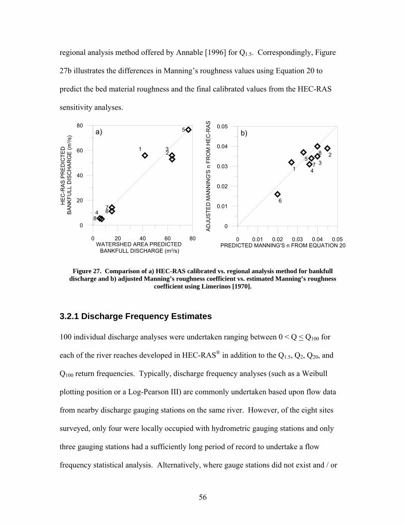
56

regional analysis method offered by Annable [1996] for Q1.5. Correspondingly, Figure

27b illustrates the differences in Manning’s roughness values using Equation 20 to

predict the bed material roughness and the final calibrated values from the HEC-RAS

sensitivity analyses.

0 0.01 0.02 0.03 0.04 0.05PREDICTED MANNING'S n FROM EQUATION 20

0

0.01

0.02

0.03

0.04

0.05

AD

JUS

TED

MA

NN

ING

'S n

FR

OM

HE

C-R

AS

5

6

7

8

1

23

4

0 20 40 60 80WATERSHED AREA PREDICTED

BANKFULL DISCHARGE (m3/s)

0

20

40

60

80

HE

C-R

AS

PR

ED

ICTE

D

BAN

KFU

LL D

ISC

HA

RG

E (m

3 /s)

5

67

8

123

4

a) b)

Figure 27. Comparison of a) HEC-RAS calibrated vs. regional analysis method for bankfull discharge and b) adjusted Manning’s roughness coefficient vs. estimated Manning’s roughness

coefficient using Limerinos [1970].

3.2.1 Discharge Frequency Estimates 100 individual discharge analyses were undertaken ranging between 0 < Q < Q100 for

each of the river reaches developed in HEC-RAS® in addition to the Q1.5, Q2, Q20, and

Q100 return frequencies. Typically, discharge frequency analyses (such as a Weibull

plotting position or a Log-Pearson III) are commonly undertaken based upon flow data

from nearby discharge gauging stations on the same river. However, of the eight sites

surveyed, only four were locally occupied with hydrometric gauging stations and only

three gauging stations had a sufficiently long period of record to undertake a flow

frequency statistical analysis. Alternatively, where gauge stations did not exist and / or

57

DAbaQx loglog +=

gauges with too short of a time record to predict return frequencies or to calibrate rating

curves, the watershed drainage area was used in conjunction with regionalization

methods to predict flood flow recurrence intervals.

Regionalization techniques provided by Gingras et al. [1994] were employed to

determine the Q2, Q20 and Q100 return periods. These techniques relate particular flood

quantiles to the effective drainage areas within the provinces of Ontario and Quebec

using the equation:

[ 21 ]

where Qx [L3/T]is the flood flow of return period x [T], DA is the effective drainage area

[L2] of the watershed, and parameters a and b are regression coefficients specific to the

hydrophysiographic region. For the purposes of this study and hydrogeographic region,

Region 7 and 8 coefficients for a and b specified by Gingras et al. [1994] were utilized.

In the case of bankfull discharge (QBF), a similar regionalization technique was offered

for southern Ontario by Annable [1996] of the form:

.[ 22 ]

Annable [1996] also identified that QBF≈Q1.5 for rural rivers in southern Ontario.

Drainage areas for each site were obtained through hydrological analysis of digital

elevation models (DEMs) at 10m2 grid scales. Hydrological analyses were performed

using ArcGIS 9.1®, and the DEMs obtained from the Geological Survey of Canada to

delineate the effective catchment areas. Figure 28 illustrates an example of effective

catchment area delineation for the Conestoga River at Hawkesville. Based upon the

74.052.0 DAQBF =

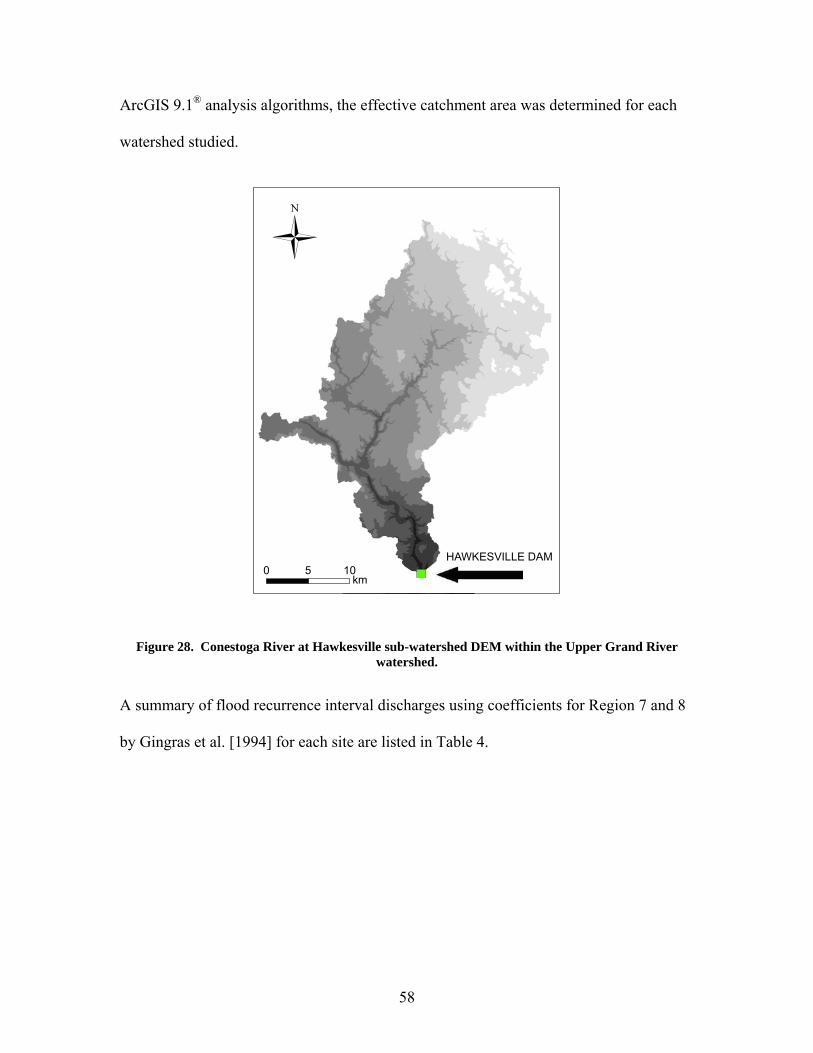
58

ArcGIS 9.1® analysis algorithms, the effective catchment area was determined for each

watershed studied.

")"")0 105km

­

HAWKESVILLE DAM

Figure 28. Conestoga River at Hawkesville sub-watershed DEM within the Upper Grand River watershed.

A summary of flood recurrence interval discharges using coefficients for Region 7 and 8

by Gingras et al. [1994] for each site are listed in Table 4.

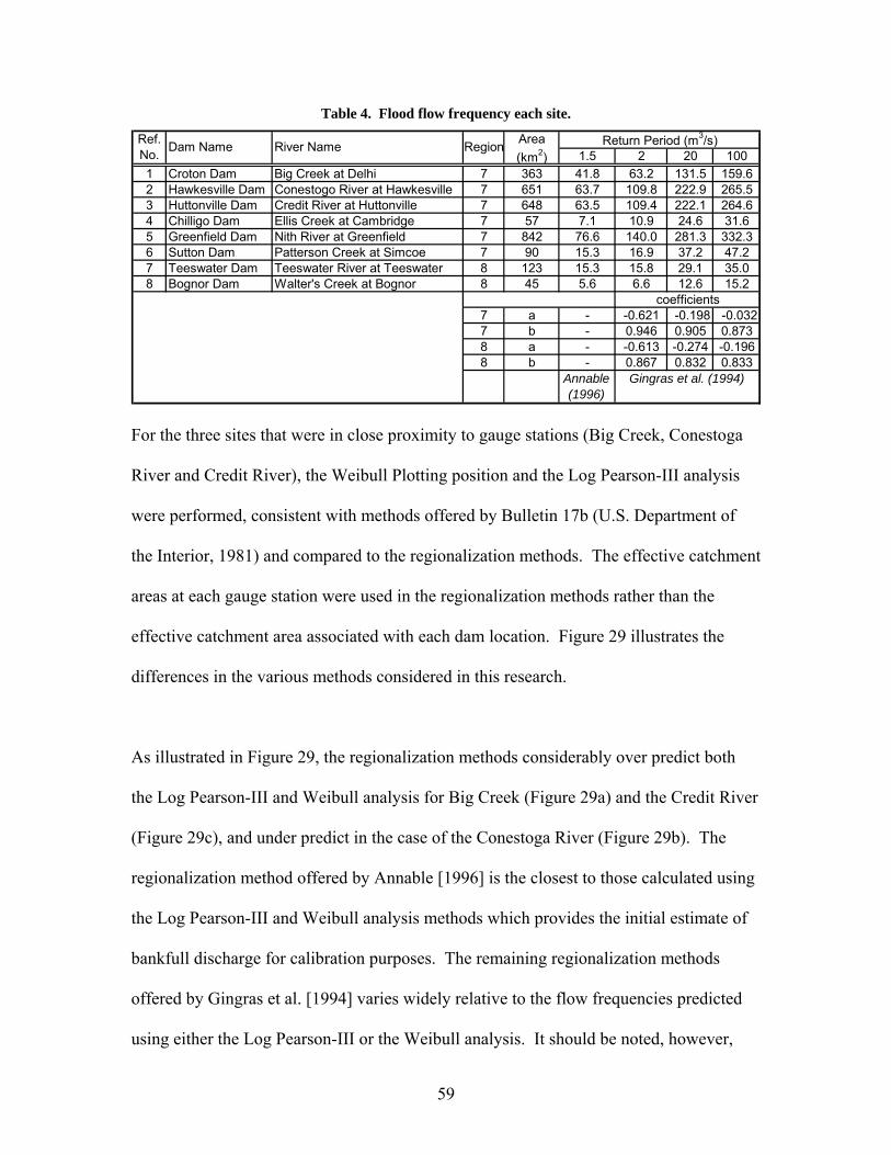
59

Table 4. Flood flow frequency each site.

1.5 2 20 1001 Croton Dam Big Creek at Delhi 7 363 41.8 63.2 131.5 159.62 Hawkesville Dam Conestogo River at Hawkesville 7 651 63.7 109.8 222.9 265.53 Huttonville Dam Credit River at Huttonville 7 648 63.5 109.4 222.1 264.64 Chilligo Dam Ellis Creek at Cambridge 7 57 7.1 10.9 24.6 31.65 Greenfield Dam Nith River at Greenfield 7 842 76.6 140.0 281.3 332.36 Sutton Dam Patterson Creek at Simcoe 7 90 15.3 16.9 37.2 47.27 Teeswater Dam Teeswater River at Teeswater 8 123 15.3 15.8 29.1 35.08 Bognor Dam Walter's Creek at Bognor 8 45 5.6 6.6 12.6 15.2

7 a - -0.621 -0.198 -0.0327 b - 0.946 0.905 0.8738 a - -0.613 -0.274 -0.1968 b - 0.867 0.832 0.833

Annable (1996)

Gingras et al. (1994)

Ref. No.

Return Period (m3/s)Dam Name River Name Area (km2)

Region

coefficients

For the three sites that were in close proximity to gauge stations (Big Creek, Conestoga

River and Credit River), the Weibull Plotting position and the Log Pearson-III analysis

were performed, consistent with methods offered by Bulletin 17b (U.S. Department of

the Interior, 1981) and compared to the regionalization methods. The effective catchment

areas at each gauge station were used in the regionalization methods rather than the

effective catchment area associated with each dam location. Figure 29 illustrates the

differences in the various methods considered in this research.

As illustrated in Figure 29, the regionalization methods considerably over predict both

the Log Pearson-III and Weibull analysis for Big Creek (Figure 29a) and the Credit River

(Figure 29c), and under predict in the case of the Conestoga River (Figure 29b). The

regionalization method offered by Annable [1996] is the closest to those calculated using

the Log Pearson-III and Weibull analysis methods which provides the initial estimate of

bankfull discharge for calibration purposes. The remaining regionalization methods

offered by Gingras et al. [1994] varies widely relative to the flow frequencies predicted

using either the Log Pearson-III or the Weibull analysis. It should be noted, however,

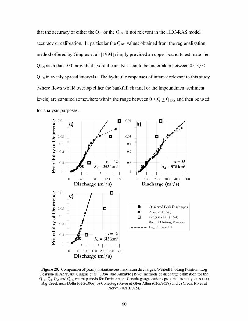
60

that the accuracy of either the Q20 or the Q100 is not relevant in the HEC-RAS model

accuracy or calibration. In particular the Q100 values obtained from the regionalization

method offered by Gingras et al. [1994] simply provided an upper bound to estimate the

Q100 such that 100 individual hydraulic analyses could be undertaken between 0 < Q <

Q100 in evenly spaced intervals. The hydraulic responses of interest relevant to this study

(where flows would overtop either the bankfull channel or the impoundment sediment

levels) are captured somewhere within the range between 0 < Q < Q100, and then be used

for analysis purposes.

0 50 100 150 200 250 300Discharge (m3/s)

1

0.5

0.2

0.1

0.05

0.01

Pro

babi

lity

of O

curr

ence

n = 12Ad = 615 km2

0 40 80 120 160Discharge (m3/s)

1

0.5

0.2

0.1

0.05

0.01

Pro

bab

ility

of O

curr

ence

n = 42Ad = 363 km2

0 100 200 300 400 500Discharge (m3/s)

1

0.5

0.2

0.1

0.05

0.01

Observed Peak DischargesAnnable (1996)Gingras et al. (1994)Weibul Plotting PositionLog Pearson III

n = 23Ad = 578 km2

a) b)

c)

Figure 29. Comparison of yearly instantaneous maximum discharges, Weibull Plotting Position, Log Pearson-III Analysis, Gingras et al. [1994] and Annable [1996] methods of discharge estimation for the Q1.5, Q2, Q20 and Q100 return periods for Environment Canada gauge stations proximal to study sites at a)

Big Creek near Delhi (02GC006) b) Conestoga River at Glen Allan (02GA028) and c) Credit River at Norval (02HB025).

61

3.2.3 Tractive Force and Permissible Velocity Analysis The stability of the bed material along a river reach is affected through shearing forces

and permissible velocity. For both shear forces and velocities, critical values were

calculated to determine the threshold values to differentiate between particle motion or

stability.

The threshold shear value (tcds), was calculated as a function of Shields parameter as

defined by Julien (1995):

[ 23 ]

Furthermore, critical shear is specific for each particle size, and in turn was calculated for

t*c5, t*c16, t*c25, t*c50, t*c75, t*c84, t*c95 particle sizes from each sample. These values

were compared to the bed shear within the main channel defined using Duboy’s equation:

[ 24 ]

which was calculated with the HEC-RAS analysis for the range of flows discussed

previously.

Critical velocities (vcids) [L T -1] were determined using the equation offered by Novak

and Nalluri [1984]:

[ 25 ]

for each of the different discharges (Qi) studied, where Ri represents the hydraulic radius

of a given hydraulic analysis at a given cross-section. As critical velocity is both a

smscdsc d)(* γγττ −=

fmo RSγτ =

)1(5.04.0

−⎟⎟⎠

⎞⎜⎜⎝

⎛=

−

GgdRd

si

sdsicv

62

function of hydraulic radius and particle size, a suite of critical velocities exist for each

flood flow and particle size respectively. The main channel velocity (Vi) and associated

hydraulic radii (Ri) calculated in HEC-RAS were used to determine the critical particle

size (dcv) that would remain stable on the channel bed for the range in discharges between

0 < Qi < Q100 using the equation defined by Novak and Nalluri [1984]:

[ 26 ]

The critical particle values for the range in flows analyzed were then compared to the

range of particle size percentiles determined by the sediment analysis (i.e. d5, d16, d25, d50,

d75, d84, d95) at each sample location to determine the particle size class associated with

the critical cessation velocity.

54

)1(4

⎟⎟⎠

⎞⎜⎜⎝

⎛−

= −

GgRi

2i

cv

Vd

63

4 RESULTS AND DISCUSSION

This chapter presents the hydraulic and sedimentological results obtained for each study

site. Unit stream power, velocity and shear stress analyses are presented for flows

ranging between 0 < Q < Q100. Subsequently, results of permissible and critical velocities

and shear stress are presented and further interpreted with respect to continued upstream

headcut migration. As all of the study sites range in longitudinal profile lengths (ranging

between 1050m and 5600m), a normalized length comparison was developed for analysis

purposes. For each study site, the distance along each thalweg longitudinal profile,

starting at the dam face, was normalized with respect to the thalweg length between the

dam face and the backwater limit of each reservoir. Using this approach, ratios of zero

and one consistently occur at the dam face and the backwater limits of the reservoirs

respectively (i.e. the region of the impoundments). Positive ratios reflect distances

progressing upstream of the dam face, whereas negative values represent reaches

progressing downstream of the dam face. The reference numbers identified in each graph

refer to each site studied as outlined in Table 2.

4.1 Upstream Disturbance Propagation

Upstream disturbances initiated from dam failure are presented using field observations

of headcuts and knickpoints. The longitudinal ratio here is defined as the maximum

upstream extent of observed headcutting, relative to the dam face, normalized by the

thalweg length of the reservoir. Figure 30 illustrates the longitudinal ratio versus the

number of years since the dam was functional.

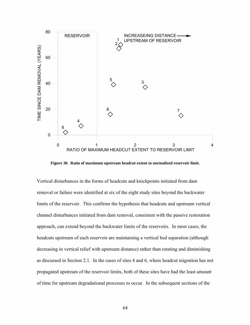
64

0 1 2 3 4RATIO OF MAXIMUM HEADCUT EXTENT TO RESERVOIR LIMIT

0

20

40

60

80

TIM

E S

INC

E D

AM

RE

MO

VA

L (Y

EAR

S)

12

3

4

5

6

78

RESERVOIR INCREASEING DISTANCE UPSTREAM OF RESERVOIR

Figure 30. Ratio of maximum upstream headcut extent to normalized reservoir limit.

Vertical disturbances in the forms of headcuts and knickpoints initiated from dam

removal or failure were identified at six of the eight study sites beyond the backwater

limits of the reservoir. This confirms the hypothesis that headcuts and upstream vertical

channel disturbances initiated from dam removal, consistent with the passive restoration

approach, can extend beyond the backwater limits of the reservoirs. In most cases, the

headcuts upstream of each reservoir are maintaining a vertical bed separation (although

decreasing in vertical relief with upstream distance) rather than rotating and diminishing

as discussed in Section 2.1. In the cases of sites 4 and 6, where headcut migration has not

propagated upstream of the reservoir limits, both of these sites have had the least amount

of time for upstream degradational processes to occur. In the subsequent sections of the

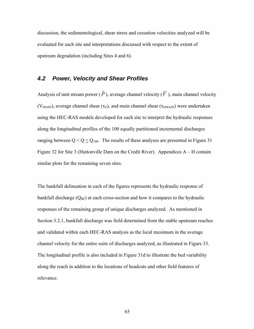
65

discussion, the sedimentological, shear stress and cessation velocities analyzed will be

evaluated for each site and interpretations discussed with respect to the extent of

upstream degradation (including Sites 4 and 6).

4.2 Power, Velocity and Shear Profiles

Analysis of unit stream power ( P ), average channel velocity (V ), main channel velocity

(VMAIN), average channel shear (τO), and main channel shear (τOMAIN) were undertaken

using the HEC-RAS models developed for each site to interpret the hydraulic responses

along the longitudinal profiles of the 100 equally partitioned incremental discharges

ranging between Q < Q < Q100. The results of these analyses are presented in Figure 31

Figure 32 for Site 3 (Huttonville Dam on the Credit River). Appendices A – H contain

similar plots for the remaining seven sites.

The bankfull delineation in each of the figures represents the hydraulic response of

bankfull discharge (QBF) at each cross-section and how it compares to the hydraulic

responses of the remaining group of unique discharges analyzed. As mentioned in

Section 3.2.1, bankfull discharge was field determined from the stable upstream reaches

and validated within each HEC-RAS analysis as the local maximum in the average

channel velocity for the entire suite of discharges analyzed, as illustrated in Figure 33.

The longitudinal profile is also included in Figure 31d to illustrate the bed variability

along the reach in addition to the locations of headcuts and other field features of

relevance.

66

It should further be noted that a longitudinal profile was not undertaken by wading the

channel for site 1 similar to the other seven sites. Rather, channel cross-sections were

surveyed using a Sokkia® Set 5E total station and their locations geo-referenced using a

differentially corrected first order accurate GPS. Cross-sections were exclusively

surveyed for this reach as there was significant tree fall (woody debris) and channel

incisement making the navigation through the channel very prohibitive over the 4km

incised channel reach.

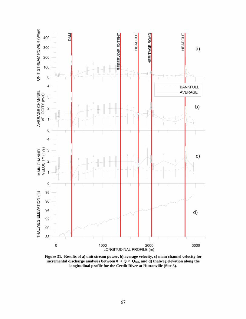
67

88

90

92

94

96

98

THA

LWE

G E

LEV

ATI

ON

(m)

DA

M

RE

SE

RVO

IR E

XTE

NT

HE

AD

CU

T

HE

AD

CU

T

HE

RIT

AG

E R

OA

D

0 1000 2000 3000LONGITUDINAL PROFILE (m)

0

1

2

3

4

MA

IN C

HA

NN

EL

VEL

OC

ITY

(m/s

)

0

1

2

3

4

AVE

RA

GE

CH

ANN

EL

VE

LOC

ITY

(m/s

)

0

100

200

300

400U

NIT

STR

EA

M P

OW

ER

(W/m

2 )

BANKFULLAVERAGE

a)

b)

c)

d)

Figure 31. Results of a) unit stream power, b) average velocity, c) main channel velocity for incremental discharge analyses between 0 < Q < Q100, and d) thalweg elevation along the

longitudinal profile for the Credit River at Huttonville (Site 3).

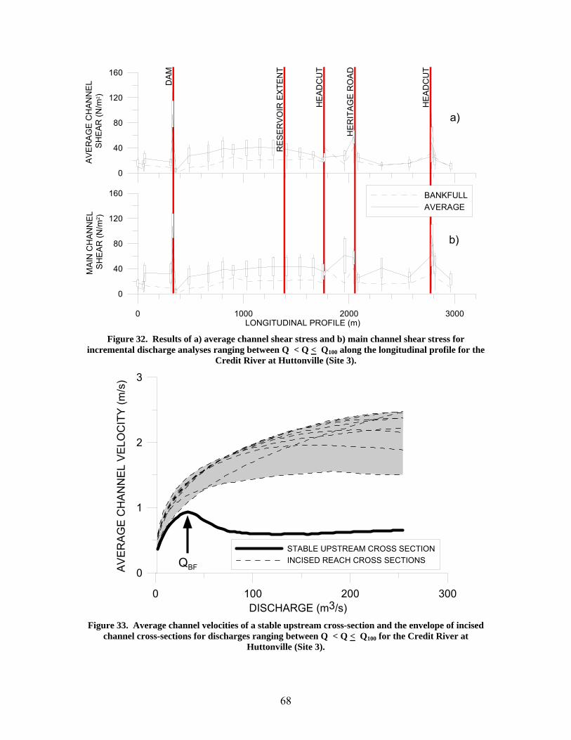
68

DA

M

RE

SE

RV

OIR

EX

TEN

T

HE

ADC

UT

HE

ADC

UT

HE

RIT

AG

E R

OA

D

0

40

80

120

160

MA

IN C

HA

NN

EL

SH

EA

R (N

/m2 )

0 1000 2000 3000LONGITUDINAL PROFILE (m)

0

40

80

120

160

AV

ER

AG

E C

HA

NN

EL

SH

EA

R (N

/m2 )

BANKFULLAVERAGE

a)

b)

Figure 32. Results of a) average channel shear stress and b) main channel shear stress for

incremental discharge analyses ranging between Q < Q < Q100 along the longitudinal profile for the Credit River at Huttonville (Site 3).

0 100 200 300DISCHARGE (m3/s)

0

1

2

3

AV

ER

AG

E C

HA

NN

EL

VE

LOC

ITY

(m/s

)

STABLE UPSTREAM CROSS SECTIONINCISED REACH CROSS SECTIONSQBF

Figure 33. Average channel velocities of a stable upstream cross-section and the envelope of incised

channel cross-sections for discharges ranging between Q < Q < Q100 for the Credit River at Huttonville (Site 3).

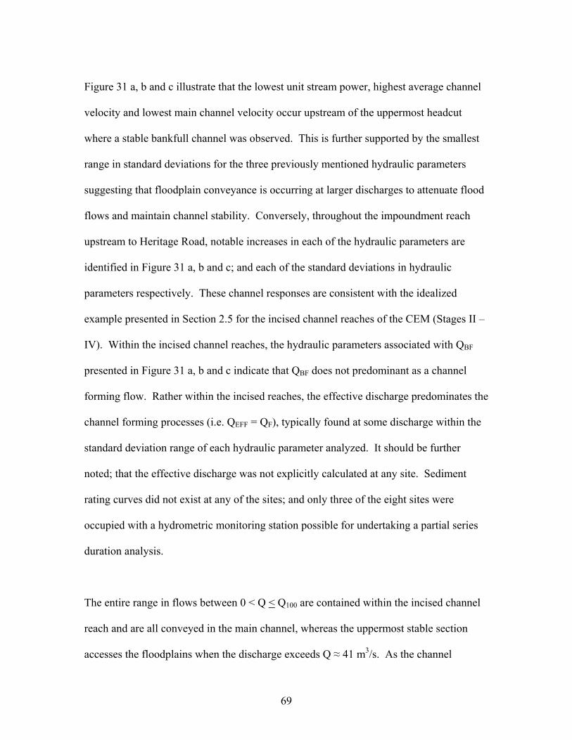
69

Figure 31 a, b and c illustrate that the lowest unit stream power, highest average channel

velocity and lowest main channel velocity occur upstream of the uppermost headcut

where a stable bankfull channel was observed. This is further supported by the smallest

range in standard deviations for the three previously mentioned hydraulic parameters

suggesting that floodplain conveyance is occurring at larger discharges to attenuate flood

flows and maintain channel stability. Conversely, throughout the impoundment reach

upstream to Heritage Road, notable increases in each of the hydraulic parameters are

identified in Figure 31 a, b and c; and each of the standard deviations in hydraulic

parameters respectively. These channel responses are consistent with the idealized

example presented in Section 2.5 for the incised channel reaches of the CEM (Stages II –

IV). Within the incised channel reaches, the hydraulic parameters associated with QBF

presented in Figure 31 a, b and c indicate that QBF does not predominant as a channel

forming flow. Rather within the incised reaches, the effective discharge predominates the

channel forming processes (i.e. QEFF = QF), typically found at some discharge within the

standard deviation range of each hydraulic parameter analyzed. It should be further

noted; that the effective discharge was not explicitly calculated at any site. Sediment

rating curves did not exist at any of the sites; and only three of the eight sites were

occupied with a hydrometric monitoring station possible for undertaking a partial series

duration analysis.

The entire range in flows between 0 < Q < Q100 are contained within the incised channel

reach and are all conveyed in the main channel, whereas the uppermost stable section

accesses the floodplains when the discharge exceeds Q ≈ 41 m3/s. As the channel

70

velocities increase with increasing discharge for the incised channel reaches (as

illustrated in Figure 33, larger particles are able to be entrained within the bedload

transport fractions. The velocities within the incised channel reach are compared to those

where bankfull discharge (and its associated velocity as illustrated in Figure 33) dominate

the channel evolution in a floodplain channel morphology. As a result of the differences

between velocities in the incised vs. bankfull reaches, and in turn the sizes and the mass

of material able to be transported in each reach, a discontinuity exists in sediment

transport from the upstream stable to incised channel reaches. Since the upstream

reaches are not able to transport sufficient mass and sizes to maintain sediment continuity

within the incised channel reaches, channel degradation by mass transport ensues leading

to further channel incision and widening. This response is common to transport

regardless if the average channel velocity (Figure 33) or main channel velocities are

considered (Figure 34).

0 100 200 300DISCHARGE (m3/s)

0

0.5

1

1.5

2

2.5

3

MAI

N C

HAN

NE

L V

ELO

CIT

Y (m

/s)

STABLE UPSTREAM CROSS SECTIONINCISED REACH CROSS SECTIONS

Figure 34. Main channel velocities of a upstream stable cross-section and the envelope of incised

cross-sections for discharges ranging between Q < Q < Q100 for Site 3.

71

Upon detailed examination of the longitudinal profile in Figure 31d, channel bed slope

(So) within the reservoir was calculated at S0 = 0.33% as compared to the adjacent valley

slope of SV = 0.27%. Channel slopes greater than their associated valley slopes are

another indicator of channel degradation consistent with Stages II and III channel

evolution. In stable river channels, the channel bed slope is always less than or equal to

the valley slope (i.e. SO > SV) by reason of meander bend extension. The increase in

localized bed slope through the incised reaches results in increased hydraulic responses of

stream power and channel velocities potentially in excess of the surrounding geological

material incipient thresholds that were deposited over centuries. Over geologic time

lines, the stable bed material size and channel slope evolve to a condition whereby SO >

SV, which is not the case in the incised channel reaches. Along the increased channel

slope associated with headcut migration, the critical particle size thresholds may be

exceeded to erode particles otherwise stable; leading to continued channel degradation.

These results will be presented in Section 4.3.

Figure 32a and Figure 32b illustrate the average and main channel shear stress

respectively along the channel profile in a similar hydraulic fashion to Figure 31a through

Figure 31c. When discharges exceed QBF in the floodplain dominated morphology, the

wetted perimeter (Λ) significantly increases with inverse affects on the hydraulic radius

(R) resulting in shear stresses remaining relatively low for the entire range of flows.

Conversely, in the cross-sections where flows exceed QBF and do not access their

adjacent floodplains, flow depths continue to increase with discharge and Λ increases at a

relatively lower rate to that of the stable channels reaches until overbank access is

72

attained. This results in main channel shear (τOMAIN) and average channel shear (τO)

continuously increasing until floodplains are accessed where Λ significantly increases.

Moreover, there is an increased tendency in the incised sections for channel degradation

to occur as shear thresholds are more likely to be exceeded as a result of increasing

hydraulic radii relative to the bed material sizes and cohesiveness required to maintain

channel bed and bank stability.

Hydraulic responses for P , V , VMAIN, τOAVERAGE, and τOMAIN for the seven other sites

are included in Appendices A – H. The hydraulic responses of the seven other sites

studied are thematically similar to Site 3 (Huttonville Dam on the Credit River) which are

presented in Figure 31 and Figure 32.

To further summarize the effects of vertical channel degradation identified by migrating

headcuts, plots were constructed which illustrate P (Figure 35 ), V and VMAIN (Figure

36), τO and τOMAIN (Figure 37) for the discharge at each channel cross-section when

overbank cresting occurs (i.e. when water begins to spill out onto the adjacent flood

plain) for all of the river reaches studied. In the cases of the bankfull channel reaches,

this discharge is synonymous with QBF. Within the incised channel reaches, the

discharge used in the analyses is the unique flow observed when an inflection occurs in

the average velocity vs. discharge plots for each cross-section (similar to those presented

in Figure 33 and Figure 34) and/or where a notable increase in top widths occurred with

increasing discharge. In the event that a channel inflection does not occur at a given

cross-section, the Q100 discharge was used in the analysis. Ratios greater than 1.0 on the

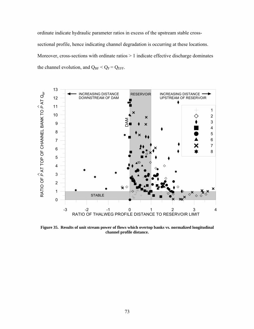
73

ordinate indicate hydraulic parameter ratios in excess of the upstream stable cross-

sectional profile, hence indicating channel degradation is occurring at these locations.

Moreover, cross-sections with ordinate ratios > 1 indicate effective discharge dominates

the channel evolution, and QBF < QF = QEFF.

-3 -2 -1 0 1 2 3 4RATIO OF THALWEG PROFILE DISTANCE TO RESERVOIR LIMIT

0

1

2

3

4

5

6

7

8

9

10

11

12

13

RA

TIO

OF

P A

T TO

P O

F C

HA

NN

EL

BAN

K T

O P

AT

QB

F

12345678

INCREASING DISTANCE DOWNSTREAM OF DAM

RESERVOIR INCREASING DISTANCE UPSTREAM OF RESERVOIR

STABLE

DA

M

Figure 35. Results of unit stream power of flows which overtop banks vs. normalized longitudinal channel profile distance.

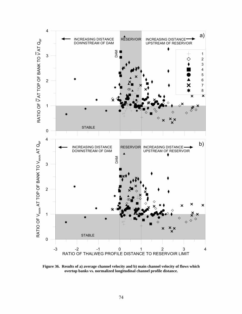
74

-3 -2 -1 0 1 2 3 4RATIO OF THALWEG PROFILE DISTANCE TO RESERVOIR LIMIT

0

1

2

3

4

RA

TIO

OF

VM

AIN

AT

TOP

OF

BAN

K T

O V

MA

IN A

T Q

BFINCREASING DISTANCEDOWNSTREAM OF DAM

RESERVOIR INCREASING DISTANCEUPSTREAM OF RESERVOIR

0

1

2

3

4

RA

TIO

OF

V A

T TO

P O

F B

ANK

TO V

AT

QBF

12345678

DAM

DAM

STABLE

STABLE

a)

b)INCREASING DISTANCEDOWNSTREAM OF DAM

RESERVOIR INCREASING DISTANCEUPSTREAM OF RESERVOIR

Figure 36. Results of a) average channel velocity and b) main channel velocity of flows which overtop banks vs. normalized longitudinal channel profile distance.

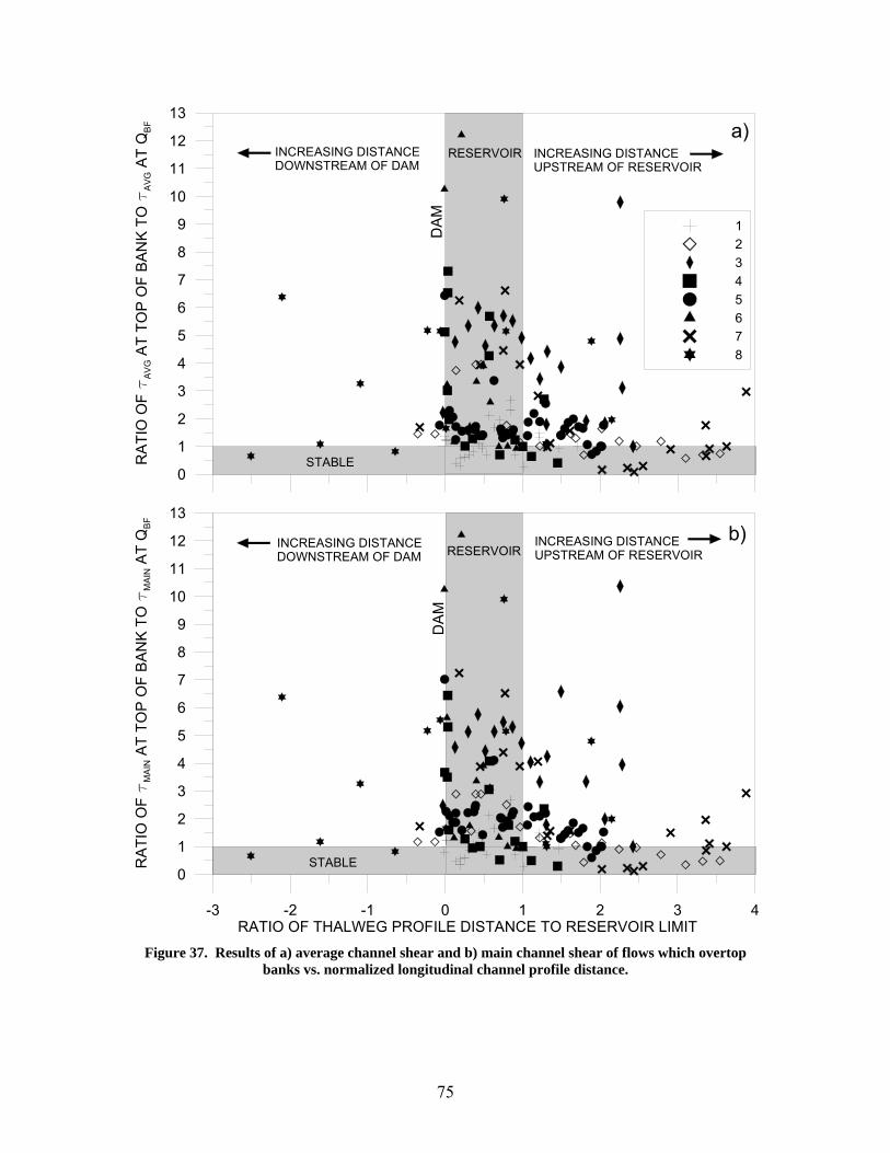
75

INCREASING DISTANCEDOWNSTREAM OF DAM

RESERVOIR INCREASING DISTANCEUPSTREAM OF RESERVOIR

-3 -2 -1 0 1 2 3 4RATIO OF THALWEG PROFILE DISTANCE TO RESERVOIR LIMIT

0

1

2

3

4

5

6

7

8

9

10

11

12

13

RA

TIO

OF t

MA

IN A

T TO

P O

F B

AN

K T

O t

MA

IN A

T Q

BF

0

1

2

3

4

5

6

7

8

9

10

11

12

13

RA

TIO

OF t

AV

G A

T TO

P O

F B

AN

K T

O t

AVG

AT

QB

F

12345678

STABLE

DA

M

STABLE

DA

M

a)

b)INCREASING DISTANCE DOWNSTREAM OF DAM RESERVOIR

INCREASING DISTANCEUPSTREAM OF RESERVOIR

Figure 37. Results of a) average channel shear and b) main channel shear of flows which overtop

banks vs. normalized longitudinal channel profile distance.

76

The hydraulic parameter ( P , V , VMAIN, τO, τOMAIN) responses at each site are similar,

with the exception of site 1, and maintain ratios >1 on the ordinate immediately upstream

of the dam, indicative of channel evolution Stages II - III. Elevated hydraulic

characteristics at flows that overtop banks above bankfull discharge are consistent with

incised channels causing increased sediment carrying capacity and decreased channel

sinuosity resulting in steeper bed slopes or some combination thereof. Where ratios

exceed unity, effective discharge dominates the channel evolution. Additionally, at these

cross-sections there is an increased tendency for further channel degradation to occur, as

thresholds of greater particle sizes and cohesiveness are exceeded for flows greater than

bankfull. The trend of cross-sections tends towards unity with increasing distance

upstream of the reservoir.

Site 1 is the exception in the hydraulic responses relative to the other seven sites.

Examining the cross-sections for site 1 immediately upstream of the dam in Figures 35,

Figure 36 and Figure 37, overbank flow ratios are < 1. These cross-sections have been

evolving for approximately 70 years (since the time of failure) and demonstrate Stage IV

or Stage V characteristics. As cross-sections are examined in sequence of increasing

distance upstream from the dam, the effects of incision gradually increase (tending

towards stages III and II of the CEM sequence). Moreover, Figure 6b in Section 2.3

demonstrates this longitudinal evolution of channel morphology, where downstream

reaches are in a state of quasi-equilibrium and upstream reaches are increasing in both

vertical and cross-sectional profiles consistent with the location of the uppermost

headcut.

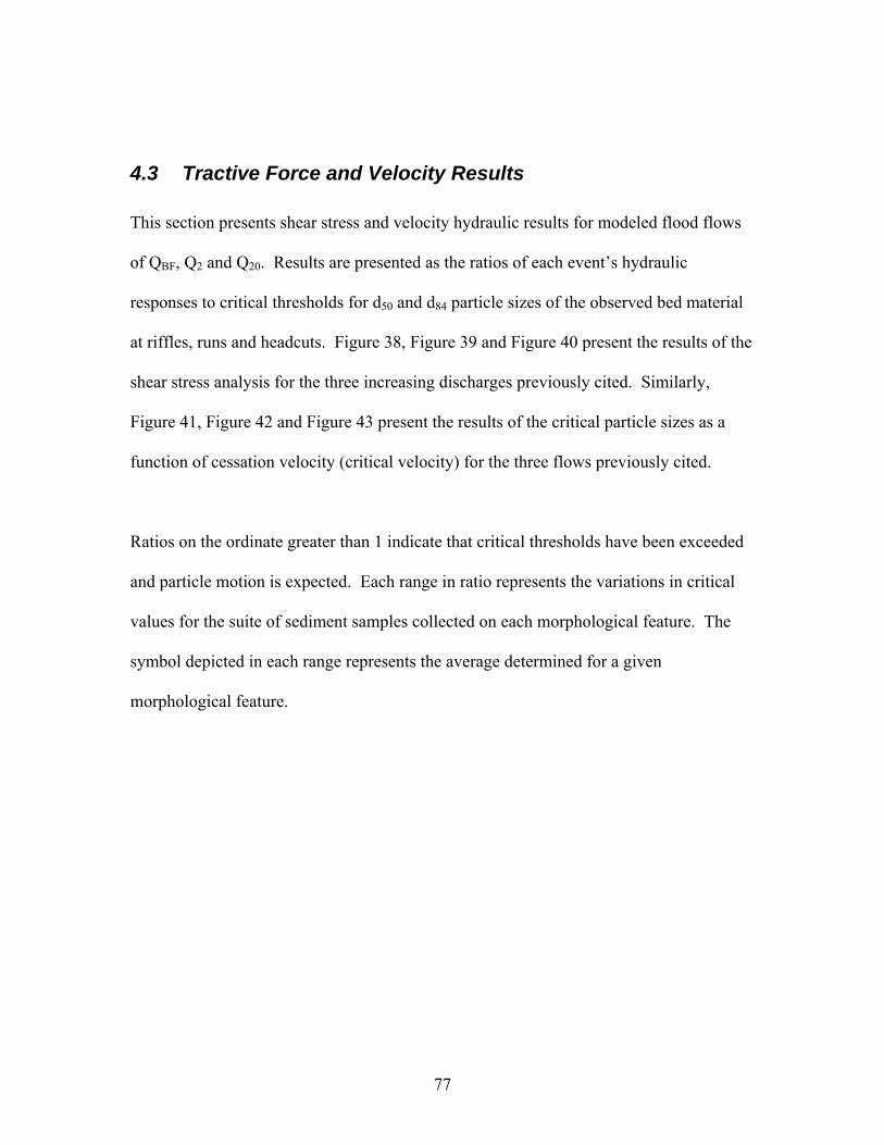
77

4.3 Tractive Force and Velocity Results

This section presents shear stress and velocity hydraulic results for modeled flood flows

of QBF, Q2 and Q20. Results are presented as the ratios of each event’s hydraulic

responses to critical thresholds for d50 and d84 particle sizes of the observed bed material

at riffles, runs and headcuts. Figure 38, Figure 39 and Figure 40 present the results of the

shear stress analysis for the three increasing discharges previously cited. Similarly,

Figure 41, Figure 42 and Figure 43 present the results of the critical particle sizes as a

function of cessation velocity (critical velocity) for the three flows previously cited.

Ratios on the ordinate greater than 1 indicate that critical thresholds have been exceeded

and particle motion is expected. Each range in ratio represents the variations in critical

values for the suite of sediment samples collected on each morphological feature. The

symbol depicted in each range represents the average determined for a given

morphological feature.

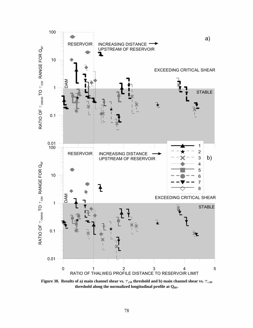
78

STABLE

EXCEEDING CRITICAL SHEAR

RESERVOIR INCREASING DISTANCEUPSTREAM OF RESERVOIR

0.01

0.1

1

10

100

RA

TIO

OF t

OM

AIN

TO

tC

50 R

AN

GE

FO

R Q

BF

a)

DA

M

RESERVOIR INCREASING DISTANCE UPSTREAM OF RESERVOIR

0 1 2 3 4 5RATIO OF THALWEG PROFILE DISTANCE TO RESERVOIR LIMIT

0.01

0.1

1

10

100

RA

TIO

OF t

OM

AIN

TO

tC

84 R

AN

GE

FO

R Q

BF

12345678

STABLE

EXCEEDING CRITICAL SHEAR

b)

DAM

Figure 38. Results of a) main channel shear vs. tc50 threshold and b) main channel shear vs. tc 84

threshold along the normalized longitudinal profile at QBF.

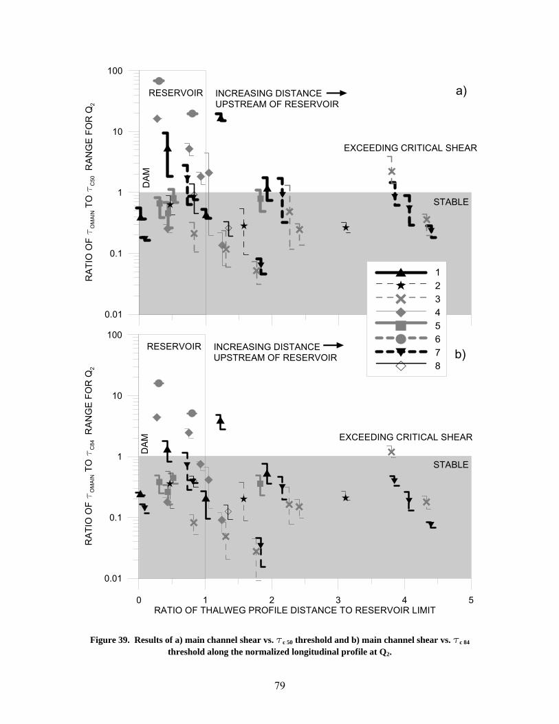
79

RESERVOIR INCREASING DISTANCE UPSTREAM OF RESERVOIR

0.01

0.1

1

10

100

RA

TIO

OF t

OM

AIN T

O t

C50

RA

NG

E F

OR

Q2

12345678

STABLE

EXCEEDING CRITICAL SHEAR

a)

DA

M

RESERVOIR INCREASING DISTANCE UPSTREAM OF RESERVOIR

0 1 2 3 4 5RATIO OF THALWEG PROFILE DISTANCE TO RESERVOIR LIMIT

0.01

0.1

1

10

100

RAT

IO O

F t

OM

AIN

TO

tC

84 R

AN

GE

FO

R Q

2

STABLE

EXCEEDING CRITICAL SHEAR

b)

DA

M

Figure 39. Results of a) main channel shear vs. tc 50 threshold and b) main channel shear vs. tc 84 threshold along the normalized longitudinal profile at Q2.

80

0.01

0.1

1

10

100

RA

TIO

OF t

OM

AIN

TO

tC

50 R

AN

GE

FO

R Q

20

12345678

STABLE

RESERVOIR INCREASEING DISTANCE UPSTREAM OF RESERVOIR

EXCEEDING CRITICAL SHEAR

DA

M

a)

0 1 2 3 4 5RATIO OF THALWEG PROFILE DISTANCE TO RESERVOIR LIMIT

0.01

0.1

1

10

100

RA

TIO

OF t

OM

AIN

TO

tC

84 R

AN

GE

FO

R Q

20

STABLE

RESERVOIR INCREASING DISTANCE UPSTREAM OF RESERVOIR

EXCEEDING CRITICAL SHEAR

b)

DA

M

Figure 40. Results of a) main channel shear vs. tc 50 critical threshold and b) main channel shear vs.

tc 84 critical threshold along the normalized longitudinal profile at Q20.

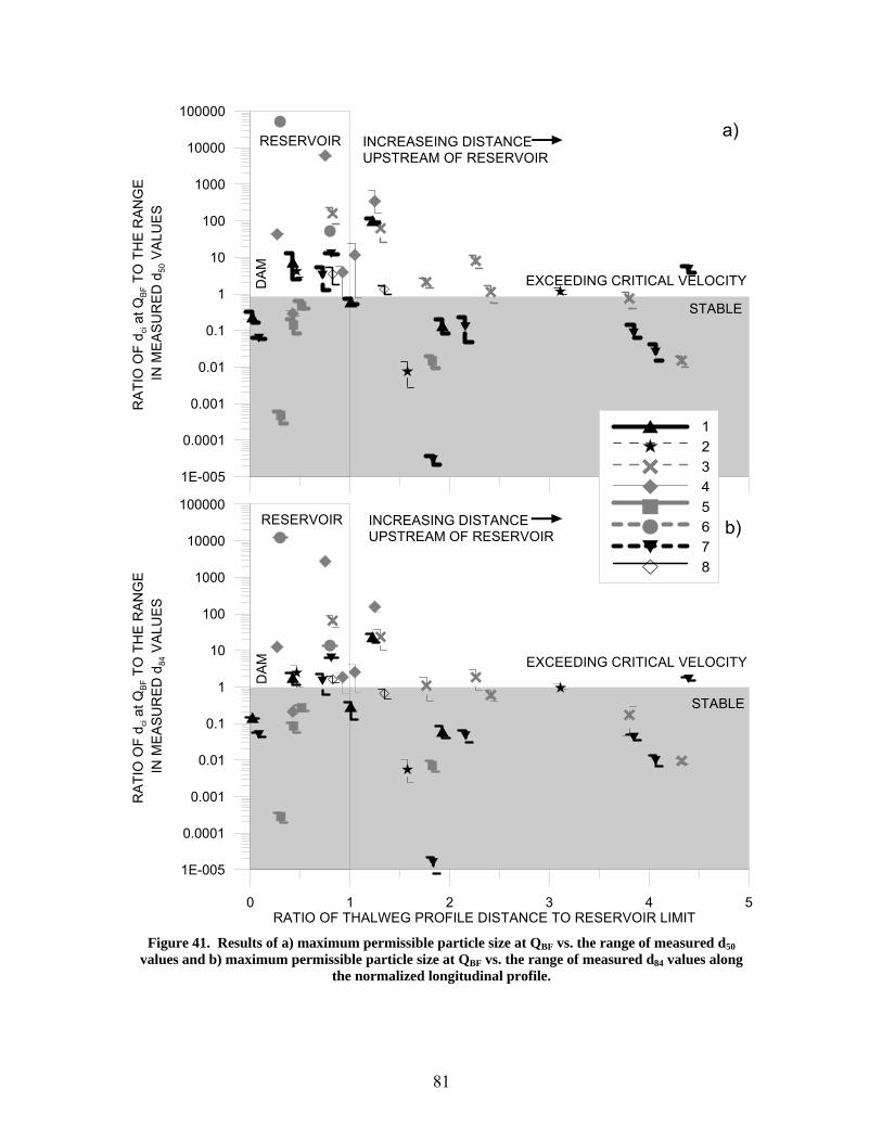
81

RESERVOIR UPSTREAM OF RESERVOIR

1E-005

0.0001

0.001

0.01

0.1

1

10

100

1000

10000

100000

RAT

IO O

F d c

i at Q

BF T

O T

HE

RAN

GE

IN

ME

ASU

RED

d50

VA

LUE

S

12345678

STABLE

RESERVOIR INCREASEING DISTANCE UPSTREAM OF RESERVOIR

EXCEEDING CRITICAL VELOCITY

a)

DA

M

0 1 2 3 4 5RATIO OF THALWEG PROFILE DISTANCE TO RESERVOIR LIMIT

1E-005

0.0001

0.001

0.01

0.1

1

10

100

1000

10000

100000

RA

TIO

OF

d ci a

t QB

F TO

TH

E R

ANG

E IN

ME

ASU

RED

d84

VAL

UES

STABLE

RESERVOIR INCREASING DISTANCEUPSTREAM OF RESERVOIR

EXCEEDING CRITICAL VELOCITY

b)

DAM

Figure 41. Results of a) maximum permissible particle size at QBF vs. the range of measured d50

values and b) maximum permissible particle size at QBF vs. the range of measured d84 values along the normalized longitudinal profile.

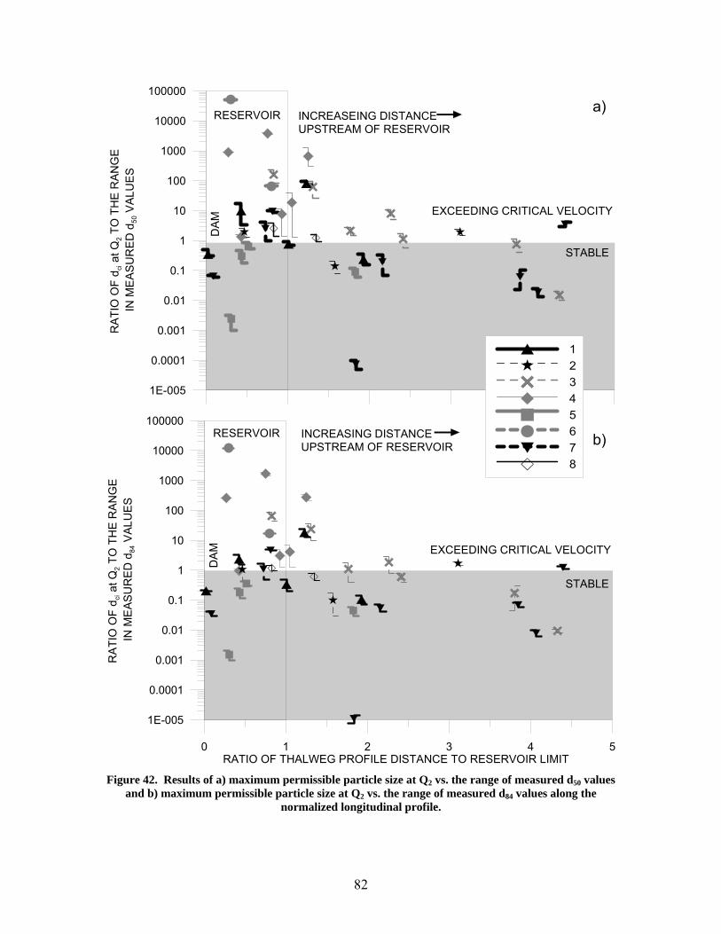
82

RESERVOIR UPSTREAM OF RESERVOIR

1E-005

0.0001

0.001

0.01

0.1

1

10

100

1000

10000

100000

RAT

IO O

F d c

i at Q

2 TO

TH

E R

AN

GE

IN

ME

ASU

RED

d50

VAL

UE

S

12345678

STABLE

RESERVOIR INCREASEING DISTANCE UPSTREAM OF RESERVOIR

EXCEEDING CRITICAL VELOCITY

a)

DA

M

0 1 2 3 4 5RATIO OF THALWEG PROFILE DISTANCE TO RESERVOIR LIMIT

1E-005

0.0001

0.001

0.01

0.1

1

10

100

1000

10000

100000

RA

TIO

OF

d ci a

t Q2 T

O T

HE

RA

NG

E

IN M

EAS

UR

ED d

84 V

ALU

ES

STABLE

RESERVOIR INCREASING DISTANCEUPSTREAM OF RESERVOIR

EXCEEDING CRITICAL VELOCITY

b)

DA

M

Figure 42. Results of a) maximum permissible particle size at Q2 vs. the range of measured d50 values

and b) maximum permissible particle size at Q2 vs. the range of measured d84 values along the normalized longitudinal profile.

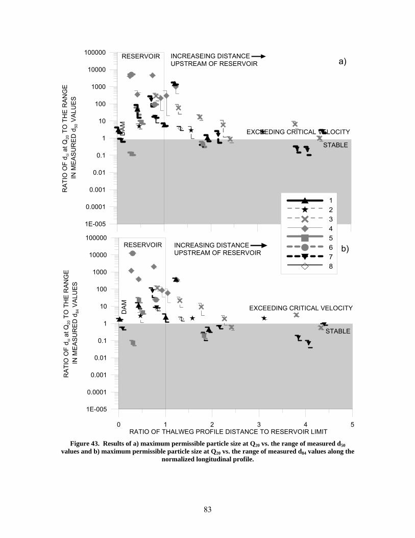
83

RESERVOIR UPSTREAM OF RESERVOIR

1E-005

0.0001

0.001

0.01

0.1

1

10

100

1000

10000

100000

RA

TIO

OF

d ci a

t Q20

TO

TH

E R

AN

GE

IN

ME

AS

UR

ED

d50

VA

LUE

S

12345678

STABLE

RESERVOIR INCREASEING DISTANCE UPSTREAM OF RESERVOIR

EXCEEDING CRITICAL VELOCITY

a)

DA

M

0 1 2 3 4 5RATIO OF THALWEG PROFILE DISTANCE TO RESERVOIR LIMIT

1E-005

0.0001

0.001

0.01

0.1

1

10

100

1000

10000

100000

RA

TIO

OF

d ci a

t Q20

TO

TH

E R

AN

GE

IN

ME

AS

UR

ED

d84

VA

LUES

STABLE

RESERVOIR INCREASING DISTANCEUPSTREAM OF RESERVOIR

EXCEEDING CRITICAL VELOCITY

b)

DA

M

Figure 43. Results of a) maximum permissible particle size at Q20 vs. the range of measured d50

values and b) maximum permissible particle size at Q20 vs. the range of measured d84 values along the normalized longitudinal profile.

84

A common trend observed in Figure 38 – Figure 43 is that with increasing discharge, a

greater number of the morphological features (i.e. headcuts, runs and riffles) begin to

incrementally exceed both their critical shear stress and velocity thresholds. As many of

the sites range in age between 2 years and 20 years, continued and enhanced channel

degradation is predicted with the hydraulic responses between the Q2 and Q20 year

return periods. Further, the general trends presented in Figure 38 – Figure 43 also

indicate that, in most cases, the particle sizes comprising the bed material, and their

associated critical thresholds, are more often exceeded relative to the critical shear

thresholds for the range in flows studied.

General trends, most apparent within the velocity results for Q20 (Figure 43) illustrate

higher surpluses in the permissible thresholds of particles within the incised sections of

the reservoir compared to cross-sections upstream with less incision. Within the

reservoir, the greatest surpluses (greatest ratios) occur at sites 6 and 4; the youngest two

dam failure sites. This is consistent among the results of shear and velocity. The

analyses of morphological features within the reservoir at both of these sites are

experiencing the effects of Stage II channel evolution. Sites 4 and 6 are still evolving as

the maximum upstream headcut at both sites have not surpassed the reservoir limit. In

turn, the most recently removed dams show the greatest susceptibility to erosion during

floods within the reservoir caused by highly incised, low sinuosity channels. This

susceptibility will be maintained until the channel widens and increases in sinuosity,

indicative of later stages of channel evolution.

85

The uppermost feature for each site indicates the sediment range of the stable bankfull

morphology which has yet to be affected by vertical incision. Figure 38a demonstrates

that at QBF, the shear along the channel bed is insufficient to degrade the stable bankfull

morphology d50 particles at six of the eight sites (2, 3, 4, 5, 7, and 8). Moreover, Sites 2,

3, 4, 7, and 8 experience erosion of d50 at QBF due to shear at some features downstream.

These observations support the hypothesis that sediment discontinuities of d50 particles at

QBF are occurring at five of the sites. These discontinuities cause further degradation of

the channel bed and banks, and are a principle driving force in headcut migration.

It was mentioned in Section 4.2 that Site 1 cross-sections immediately upstream of the

dam had evolved to later stages of channel evolution (Stage IV or V) and experienced

low hydraulic responses to floods attributed to floodplain access at lower discharge

levels. Further upstream at Site 1, however, severe channel incision is still apparent as

illustrated in Figure 38 – Figure 43 as ratios on the ordinate typically exceed unity.

These results further the conclusion as the foremost riffle upstream of the dam at Site 1

indicates stability of d50 and d84 particles with respect to shear for QBF, Q2, Q20 and

velocity for QBF and Q2. Within the incised cross-sections upstream, erosion due to the

exceedances of shear and velocity thresholds are apparent for all particles at all flood

flows.

To simplify the results presented in Figure 38 – Figure 43, the following summary tables

were prepared for the shear stress ratios (Table 5) and critical velocity ratios (Table 6).

These tables identify for each site and discharge analyzed, the particle sizes which exceed

86

their respective critical thresholds (i.e. values greater than unity in Figure 38 – Figure

43). Further, the tables have been divided into two sections to depict the erosion of the

specified particle ranges within the impoundment and upstream of the impoundment.

Table 5. Summary of bed material and sizes exceeding critical shear stress thresholds for QBF, Q2, and Q20 within and upstream of site impoundments. Note: if particle sizes are identified in the table,

they exceed critical thresholds at one or more morphological features.

Within Impoundment Upstream of Impoundment SITE QBF Q2 Q20 QBF Q2 Q20

Time Since Failure (Years)

1 d50/d84 d50/d84 d50/d84 d50/d84 d50/d84 d50/d84 70 2 d50 67 3 d50 d50 d50/d84 d50 37 4 d50/d84 d50/d84 d50/d84 d50 d50 d50 7 5 d50 d50 d50 d50 39 6 d50/d84 d50/d84 d50/d84 2 7 d50/d84 d50/d84 d50/d84 d50 d50 d50 15 8 d50 d50 d50 16

Table 6. Summary of bed material and sizes exceeding critical velocity thresholds for QBF, Q2, and Q20 within and upstream of site impoundments. Note: if particle sizes are identified in the table, they

exceed critical thresholds at one or more morphological features.

Within Impoundment Upstream of Impoundment SITE QBF Q2 Q20 QBF Q2 Q20

Channel Slope (SO)

(-) 1 d50/d84 d50/d84 d50/d84 d50/d84 d50/d84 d50/d84 - 2 d50/d84 d50/d84 d50/d84 d50/d84 d50/d84 d50/d84 3.6E-03 3 d50/d84 d50/d84 d50/d84 d50/d84 d50/d84 d50/d84 3.3E-03 4 d50/d84 d50/d84 d50/d84 d50/d84 d50/d84 d50/d84 3.8E-03 5 d50/d84 2.0E-03 6 d50/d84 d50/d84 d50/d84 8.0E-03 7 d50/d84 d50/d84 d50/d84 d50/d84 d50/d84 d50/d84 3.0E-03 8 d50/d84 d50/d84 d50/d84 d50 d50 d50/d84 8.0E-03

Comparison of Table 5 (shear) to Table 6 (velocity) show that increased levels of velocity

at flood flows have greater influences on erosion than shear stress. The notable exception

is site 5 where shear stress with increasing discharge has dominated the channel

evolution. Site 5 is located within a kame moraine deposit which has the largest source

87

of course material from upstream bank erosion (relative to the other sites), and the bed

material averages the second most coarse (d50 ≈ 69 mm – Table 3) particle size. Further,

the valley slope is the shallowest of all sites studied (1.7x10-3 m/m – Table 2) suggesting

that the combination of the course bed material sizes and the shallowest slopes would

result in velocities insufficient to typically move the range in bed material sizes.

Therefore, the predominant mechanism for Site 5 is by channel shear.

In the case of Site 6 (the most recent dam failure) headcuts have not been observed

upstream of the impoundment region. However, in undertaking the critical shear and

velocity threshold analyses, both the d50 and the d84 values exceed both critical thresholds

for all flows. Considering that the local geology of this site is a sand plain deposit and

the bed material at this site is primarily composed of sand (d50 ≈ 0.3mm – Table 3), it is

likely that this watercourse will experience continued headcutting beyond the limits of

the impoundment region. Inspection of the HEC-RAS model developed for this site

upstream of the impoundment indicates that both shear and velocity conditions for the

QBF, Q2 and Q20 exceed critical thresholds for the sand bed composition measured within

and upstream of the study site. The hydraulic analysis further supports the position that

upstream channel degradation should be expected at this river reach.

A similar argument to that posed for Site 6 is also consistent for Site 4 (which is the

second youngest dam – 7 years). The reach is a gravel bed channel (d50 ≈ 31mm – Table

3), however, as indicated in Table 5 and Table 6 the critical velocity thresholds are

exceeded throughout the impoundment and upstream regions for both d50 and d84 grain

88

sizes. Moreover, the critical shear stress thresholds for d50 and d84 are exceeded within

the impoundment in addition to the shear stress thresholds for the d50 values upstream of

the impoundment. These results suggest that headcut migration should be expected

upstream of the impoundment, however, due to the short time span since dam removal,

upstream migration has not evolved to the upper reaches.

89

5 CONCLUSIONS and RECOMMENDATIONS Field and modelling studies of eight removed or failed dam sites with no upstream

interventions were used as the analog to passive channel restoration with a headcut driven

channel formation. The results show that vertical disturbances identified by headcuts

extend for considerable distances upstream of the backwater limits of six of the eight

reservoir study sites. Furthermore, headcuts were observed and measured at all sites,

which ranged in age between 2 years – 70 years since dam failure with the likelihood in

all cases that channel degradation will continue in the future. Similar results are probable

at sites where passive dam removals are implemented without any upstream intervention.

The hydraulic responses of unit stream power, velocity and shear strength within the

disturbed channel reaches at flood flows that overtop banks were much greater than

bankfull discharges upstream of the disturbed sections. Main channel velocities

exceeding critical thresholds dominated the channel evolution processes for the range in

bed material particle sizes (0.3mm < d50 < 81mm) over critical shear stress thresholds

with increasing discharges. Only one site seems to have regained a stable channel

morphology upstream of the dam face within the reservoir – which also corresponds to

the oldest channel evolution at 70 years before present. Channel degradation and the

upstream propagation of headcuts will continue at the remaining sites until new dynamic

equilibriums are achieved when sediment and discharge continuity are established; and

geotechnical and geomorphic stability attained for each set of unique site-based

conditions.

90

5.1 Recommendations To prevent vertical disturbances of the channel bed from migrating beyond the reservoir

limits, grade control solutions should be incorporated into the channel restoration

approach to ensure that the disturbances from dam decommissioning do not propagate

upstream beyond the backwater limits. Watson and Biedenharn [1999] identified two

main categories of grade control structures which either construct a hard point within the

main channel, by increasing bed material size that exceeds both critical shear stress and

velocity thresholds, or by introducing a hydraulic control structure to decrease the energy

slope. Watson and Biedenharn [1999] further define the applicability of the type of grade

control structure depends on factors such as hydraulic conditions, sediment size, channel

morphology, and funding constraints, amongst many others. Neilson et al. [1991]

provides a comprehensive outline on types and applications of grade control structures.

If fish passage is of interest, grade control structures that facilitate this intent should be

considered. Such structures may include rocky-ramps (Newbury and Gaboury, 1993) or

cross-vane structures (Rosgen, 1996) if properly constructed within a bankfull cross-

sectional channel profile at appropriate locations.

Furthermore, the extent of base level lowering may be controlled, to reduce the energy

grade line, by a partial removal of the structure to the upper limit of the impounded

sediments. This would decrease the height of headcuts initiated at the dam face and

would increase the likelihood of them diminishing by the reservoir limits and decrease

the likelihood of velocities and shear stress exceeding critical thresholds.

91

6.0 References (AASHTO) American Association of State Highway and Transportation Officials. (2005). "A summary of existing research on low-head dam removal projects." NCHRP Project 25-25, Task 14, National Cooperative Highway Research Program, Transportation Research Board, p. 179.

Annable, W. K. (1996), Morphological relationships of rural water courses in southwestern Ontario and selected field methods in fluvial geomorphology, Ontario Ministry of Natural Resources, ISBN 077785113X, p. 92.

Arcement, G., and Schneider, V. (1989). "Guide for selecting Manning's roughness coefficients for natural channels and flood plains." U.S. Geological Survey Water Supply Paper, 2339.

Ashley, J. (2006). "The effects of small dam removal on the distribution of sedimentary contaminants." Environmental Monitoring and Assessment, 114(1), 287 - 312.

Ashmore, P. (1988). "Bed load transport in braided gravel-bed stream models." Earth Surface Processes and Landforms, 13(8), 677 - 695.

Ashworth, P. J., and Ferguson, R. I. (1989). "Size-selective entrainment of bedload in gravel-bed streams." Water Resources Research, 25(4), 627 - 634.

Beatty, D. A. (1984). "Channel migration and incision of the Beatton River." Journal of Hydraulic Engineering, 110(11), 1681-1682.

Bednarek, A. T. (2001). "Undamming Rivers: A review of the ecological impacts of dam removal." Environmental Management, 27(6), 803 - 814.

Beechie, T. T., Pollock, M. M., and Baker, S. (2007). "Channel incision, evolution and potential recovery in the Walla Walla and Tucannon River basins, northwestern USA." Earth Surface Processes and Landforms.

Begin, Z., Meyer, D., and Schumm, S. (1980). "Knickpoint migration due to baselevel lowering." Journal of the Waterway, Port, Coastal, and Ocean Division, 106(3), 369 - 388.

Biedenharn, D., and Copeland, R. (2000). "Effective discharge calculation." Coastal and Hydraulics Engineering Technical Notes (CHETN), 3(4), 1 - 10.

92

Brush, L. M., and Wolman, M. G. (1960). "Knickpoint behaviour in noncohesive material: a laboratory study." 71(1), 59 - 74.

Bunte, K., and Abt, S. (2001). "Sampling surface and subsurface particle-size distributions in wadable gravel- and cobble-bed streams for analysis in sediment transport, hydraulics, and streambed monitoring." Rep. No. 1, United States Department of Agriculture, Forest Service Rocky Mountain Research Station, p. 428.

Canadian Dam Association. (2005). "Dam Safety Guidelines." http://www.cda.ca (Aug. 9, 2006), p. 18.

Chapman, L. J., and Putnam, D. F. (1966). Physiography of southern Ontario, Second Edtion, University of Toronto Press, Toronto, Ontario, Canada, ISBN 0-8020-1944-7, p. 386.

Cheng, F., and Granata, T. (2004). "Monitoring and modeling sediment transport and geomorphology changes associated with dam removal." 2004 Self-Sustaining Solutions for Streams, Wetlands, and Watersheds Conference, American Society of Agricultural Engineers, St. Joseph, MI 49085-9659, United States, St Paul, MN, United States, pp. 208 - 213.

Copeland, R., Biedenharn, D., and Fischenich, J. (2000). "Channel-forming discharge." Coastal and Hydraulics Engineering Technical Notes (CHETN), 3(5), 1 - 10.

Cui, Y., Braudrick, C., and Rothert, S. (2005). "Preliminary Assessment of Sediment Transport Dynamics Following Dam Removal: A Case Study." ASCE conference proceedings - Managing Watersheds for Human and Natural Impacts: Engineering, Ecological, and Economic Challenges, 275 - 286.

Doyle, M. W. (2005). "Stream ecosystem response to small dam removal: Lessons from the Heartland." Geomorphology, 71(1), 227 - 244.

Doyle, M. W., Stanley, E., and Harbor, J. (2002). "Geomorphic Analogies for Assessing Probable Channel Response to Dam Removal." Journal of the American Water Resources Association, 38(6), 1567 - 1579.

Doyle, M., Stanley, E., Harbor, J., and Grant, G. (2003). "Dam Removal in the United States: Emerging Needs for Science and Policy." 84(4), 29 - 36.

93

Dynesius, M. (1994). "Fragmentation and Flow Regulation of River Systems in the Northern Third of the World." Science, 266(5186), 753 - 762.

Egiazaroff, I. V. (1965). "Calculation of nonuniform sediment concentrations." Journal of Hydraulics Division Conference Proceedings Paper, 91(4), 225 - 247.

Emerson, W. (1971). "Channelization: A Case Study." Science, 173(3994), 325 - 326.

Foster, G. R. and Meyer, L. D. (1975). "Mathematical simulation of upland erosion by fundamental erosional mechanics." Proceedings of the Sediment-Yield Workshop - Present and prospective technology for predicting sediment yield and sources, USDA Sedimentation Lab., Oxford, MS, 190 - 207.

Friedman, G., and Sanders, J. (1978). Principles of sedimentology, Wiley Publisher, New York, NY, p.792.

Gingras, D., Adamowski, K., and Pilon, P. (1994). "Regional flood equations for the provinces of Ontario and Quebec." Journal of the American Water Resources Association, 30(1), 55 - 67.

Heinz Center. (2002). "Dam removal: Science and decision making." The H. John Heinz III Center for Science, Economics and the Environment, p. 221.

Hickin, E. J., and Nanson, G. C. (1975). "The character of channel migration on the Beatton River." Geological Society of America Bulletin, 86, 487 - 494.

Julien, P. Y. (1995). Erosion and Sedimentation. Cambridge University Press, New York, NY, p. 280.

Julien, P. Y. (1995). River Mechanics. Cambridge University Press, New York, NY, p. 434.

Klingeman, P., and Emmett, W. (1982). "Gravel bedload transport processes. IN - " Gravel-bed Rivers. Fluvial Processes, Engineering and Management, R.D. Hey, J.C. Bathurst and C.R. Thorne, ed., John Wiley and Sons, Chichester, pp. 141 - 179.

Komar, P. D. (1987). "Selective gravel entrainment and the empirical evaluation of flow competence." Sedimentology, 34(6), 1165 - 1176.

Kondolf, G. M. (1997). "Hungry water: Effects of dams and gravel mining on river channels." Environmental Management, 21(4), 533 - 551.

94

Kuhnle, R. A. (1992). "Fractional transport rates of bedload on Goodwin Creek." Dynamics of gravel-bed rivers, P. Billi, ed., John Wiley and Sons Ltd, New York, 141-155.

Lane, E. W. (1955). "Design of stable alluvial channels." Transactions of American Society of Civil Engineers, 120, 1234-1260.

Leopold, L., Wolman, M., and Miller, J. (1964). Fluvial Processes in Geomorphology. W. H. Freeman and Company, San Francisco, p. 522.

Ligon, F. K. (1995). "Downstream ecological effects of dams." BioScience, 45(3), 183.

Limerinos, J. T. (1970). "Determination of the Manning coefficient from measured bed roughness in natural channels." U.S. Geological Survey Water Supply Paper, 1898-B.

MacBroom, J. G. (2005). "Evolution of channels upstream of dam removal sites." 2005 Watershed Management Conference - Managing Watersheds for Human and Natural Impacts: Engineering, Ecological, and Economic Challenges, Jul 19-22 2005, American Society of Civil Engineers, Reston, VA 20191-4400, United States, Williamsburg, VA, United States, 287-298.

Marsh, N. A. (2004). "Comparison of Methods for Predicting Incipient Motion for Sand Beds." Journal of Hydraulic Engineering, 130(7), 616 - 621.

Nanson, G. C., and Hickin, E. J. (1983). "Channel migration and incision on the Beatton River." Journal of Hydraulic Engineering, 109(3), 327-334.

Neilson, F. M., Waller, T. N., and Kennedy, K. M. (1991). "Annotated bibliography on grade control structures." Technical Report HL-91-4, U.S. Army Corps of Engineers, Waterways Experiment Station, Vicksburg, MS.

Newbury, R., and Gaboury, M. N. (1993). Stream analysis and fish habitat design : a field manual. Newbury Hydraulics, Gibsons, B.C., p. 256

Novak, P., and Nalluri, C. (1984). "Incipient motion of sediment particles over fixed beds." Journal of Hydraulic Research, 22(3), 181 - 197.

Pansic, N., Austin, R. J., and Finis, M. (1998). "Sediment management for dam decommissioning." U.S Conference on Large Dams, Sediment Management and Erosion Control on Water Resources Projects, 15th Annual USCOLD Lecture Series. San Francisco, CA. 29-45. May 15-19.

95

Papanicolaou, A. N. (2002). "Stochastic Incipient Motion Criterion for Spheres under Various Bed Packing Conditions." Journal of Hydraulic Engineering, 128(4), 369 - 380.

Petts, G. (1984). Impounded Rivers: Perspectives for ecological management. John Wiley and Sons, Chichester, England, p. 326.

Pohl, M. M. (2002). "Bringing down our dams: Trends in American dam removal rationales." Journal of the American Water Resources Association, 38(6), 1511 - 1519.

Rosgen, D. L. (1996). Applied river morphology. Wildland Hydrology, Pagosa Springs, CO. USA., ISBN # 0965328902, p. 390.

Schumm, S. (1969). "River Metamorphisis." Proceedings of the American Society of Civil Engineers, 95(6352), 255 - 273.

Schumm, S. A., Harvey, M. D., and Watson, C. C. (1984). Incised channels: morphology, dynamics, and control. Water Resources Publications, Littleton, CO. USA., p.200.

Selle, A., Burke, M., Melchior, M., and Koonce, G. (2007). "Active vs. passive channel recovery following dam removal: a comparison of approaches”, World Environmental and Water Resources Congress 2007, American Society of Civil Engineers, 243(40927), 356 - 366.

Shields, A. (1936). "Application of similarity principles and turbulence research to bed-load movement." Mitteilunger Der Preussischen Versuchsanstalt f¨ur Wasserbau Und Schiffbau, 26, 5 - 24.

Shields, F. D., Simon, A., and Steffen, L. (2000). "Reservoir effects on downstream river channel migration." Environmental Conservation, 27(1), 54 - 66.

Shvidchenko, A. B., Pender, G., and Hoey, T. (2001). "Critical shear stress for incipient motion of sand/gravel streambeds." Water Resources Research, 37(8), 2273-2283.

Simon, A. (1998). "Process-form interactions in unstable sand-bed river channels: A numerical modelling approach." Geomorphology, 21(2), 85 - 106.

Simon, A., and Darby, S. (1999). "The nature and significance of incised river channels." Incised River Channels: Processes, forms, engineering and management, John Wiley and Sons Ltd, West Sussex, England, pp. 3 - 34.

96

Simons, D. B. (1971). "Open Channel Flow." Introduction to fluvial processes, R. J. Chorley ed., pp.124 - 145.

Stanley, E. H., and Doyle, M. W. (2002). "Trading off: the ecological effects of dam removal." Bioscience, 52(8), 693 - 701.

Stein, O. R. (1993). "Criterion delineating the mode of headcut migration." Journal of Hydraulic Engineering, 119(1), 37 – 50.

Totz, C., and Klotz, D. (2003). Floodplain modeling using HEC-RAS. Haestad Press, Waterbury, CT. p. 696.

U.S. Department of the Interior. (1981). "Bulletin 17B: Guidelines for determining flood flow frequency." Interagency Advisory Committee on Water Data, Department of the Interior, U.S. Geological Survey, Office of Water Data Coordination, Reston, VA.

Watson, C., and Biedenharn, D. (1999). "Design and effectiveness of grade control structures in incised river channels of North Mississippi, USA. IN" Incised River Channels: Processes, forms, engineering and management, A. Simon, and S. Darby, eds., John Wiley and Sons Ltd, West Sussex, England, pp. 395 - 422.

Wilcock, P. R., and Southard, J. B. (1997). "Experimental study of incipient motion in mixed-size sediment." Water Resources Research, 24(7), 1137 - 1151.

Wohl, E. E. (2000). "Sediment deposition and transport patterns following a reservoir sediment release." Water Resources Research, 36(1), 319 - 333.

Wolman, M. G. (1954). "A method of sampling coarse river-bed material." American Geophysical Union, 35(6), 951 - 956.

Wolman, M. G., and Miller, W. P. (1960). "Magnitude and frequency of forces in geomorphic processes." Journal of Geology, 68, 54 - 74.

97

Appendices A – H

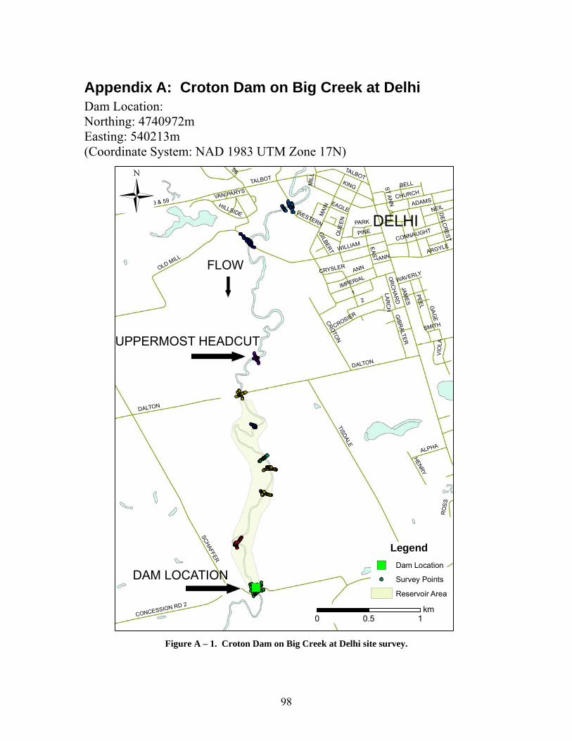
98

Appendix A: Croton Dam on Big Creek at Delhi Dam Location: Northing: 4740972m Easting: 540213m (Coordinate System: NAD 1983 UTM Zone 17N)

")

UPPERMOST HEADCUT

DELHI

JAMES

12

TISDALE

MAI

N

SCHAFFER

3 & 59

WILLIAM

CHURCH

OLD MILL

DALTON

KING

59

PEEL

CONCESSION RD 2

NORWOOD

TALBOT

QU

EEN

ANN

BELL

EAST

CROTON

GA

GE

ADAMS

PINE

CROSIER

ARGYLE

HILLSIDE

IMPERIAL

NEILWESTERN

VIO

LA

ALPHA

DELC

RES

T

HENRY

CONNAUGHT

GIBR

ALTER

OR

CH

ARD

PARK

VAN PARYS

RO

SS

EAGLE

GILBERT

SMITH

WAVERLY

MIL

L

LARC

H

CRYSLER

ST ANN

ANN

DALTON

TALBOT

­

Legend") Dam Location

Survey Points

Reservoir Area

0 10.5km

FLOW

DAM LOCATION

Figure A – 1. Croton Dam on Big Creek at Delhi site survey.

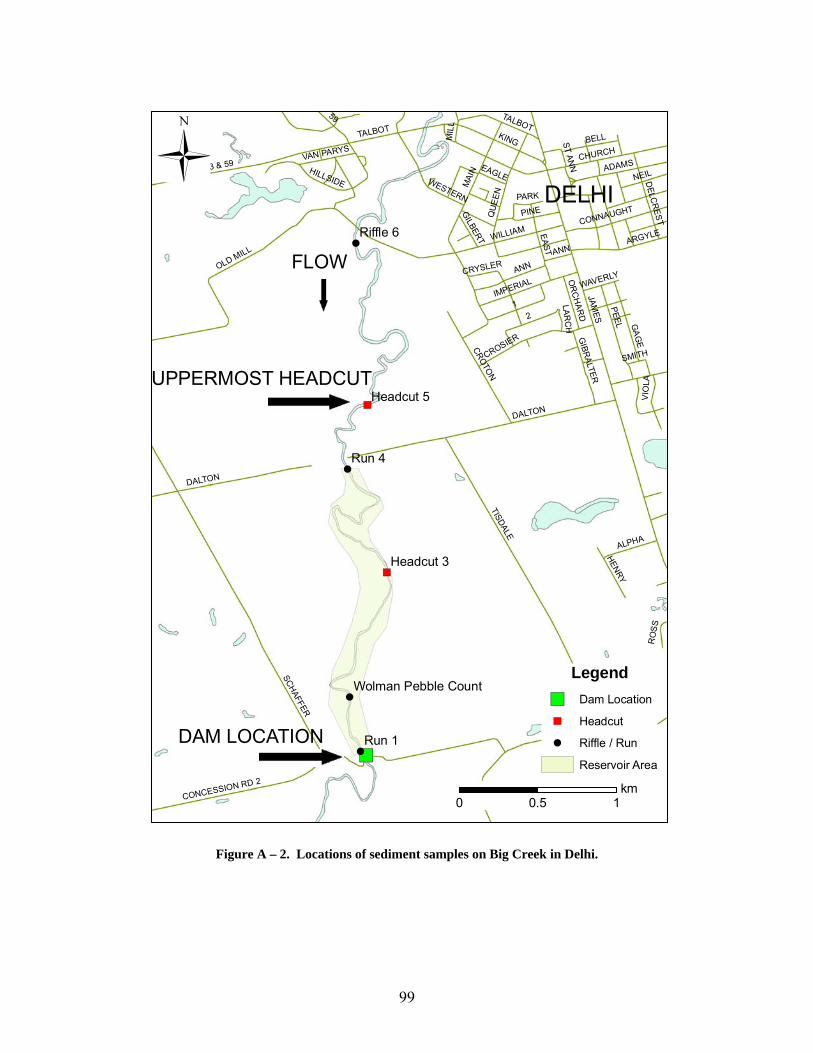
99

")!

!

!

!

")

")

UPPERMOST HEADCUT

DELHIJAM

ES

12

TISDALE

MAI

N

SCHAFFER

3 & 59

WILLIAM

CHURCH

OLD MILL

DALTON

KING

59

PEEL

CONCESSION RD 2

NORWOOD

TALBOT

QU

EEN

ANN

BELL

EAST

CROTON

GA

GE

ADAMS

PINE

CROSIER

ARGYLE

HILLSIDE

IMPERIAL

NEILWESTERN

VIO

LA

ALPHA

DELC

RES

T

HENRY

CONNAUGHT

GIBR

ALTER

OR

CH

ARD

PARK

VAN PARYS

RO

SS

EAGLE

GILBERT

SMITH

WAVERLY

MIL

L

LARC

H

CRYSLER

ST ANN

ANN

DALTON

TALBOT

Run 4

Run 1

Riffle 6

Wolman Pebble Count

Headcut 5

Headcut 3

­

Legend") Dam Location

") Headcut

! Riffle / Run

Reservoir Area

0 10.5km

FLOW

DAM LOCATION

Figure A – 2. Locations of sediment samples on Big Creek in Delhi.

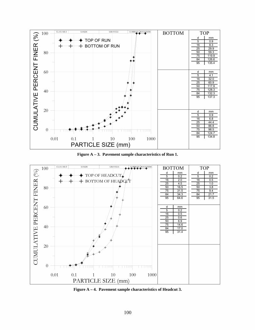
100

BOTTOM

TOP d mm5 0.916 8.325 29.950 59.375 119.984 126.695 135.4

d mm5 4.116 32.025 60.950 117.975 128.384 132.395 137.3

0.01 0.1 1 10 100 1000PARTICLE SIZE (mm)

0

20

40

60

80

100C

UM

ULA

TIV

E P

ER

CEN

T FI

NE

R (%

)TOP OF RUNBOTTOM OF RUN

CLAY/SILT SANDS GRAVELS COBBLES BOULDERS

d mm5 0.916 6.825 44.450 86.875 98.584 124.795 134.8

Figure A – 3. Pavement sample characteristics of Run 1.

BOTTOM

d mm5 0.216 2.025 4.550 16.575 31.584 34.395 64.6

TOP d mm5 0.216 0.525 1.050 3.875 9.484 21.795 31.5

d mm5 0.216 0.525 0.650 6.975 14.684 17.095 31.4

0.01 0.1 1 10 100 1000PARTICLE SIZE (mm)

0

20

40

60

80

100

CUM

ULA

TIV

E P

ERC

EN

T FI

NE

R (%

)

TOP OF HEADCUTBOTTOM OF HEADCUT

CLAY/SILT SANDS GRAVELS COBBLES BOULDERS

Figure A – 4. Pavement sample characteristics of Headcut 3.

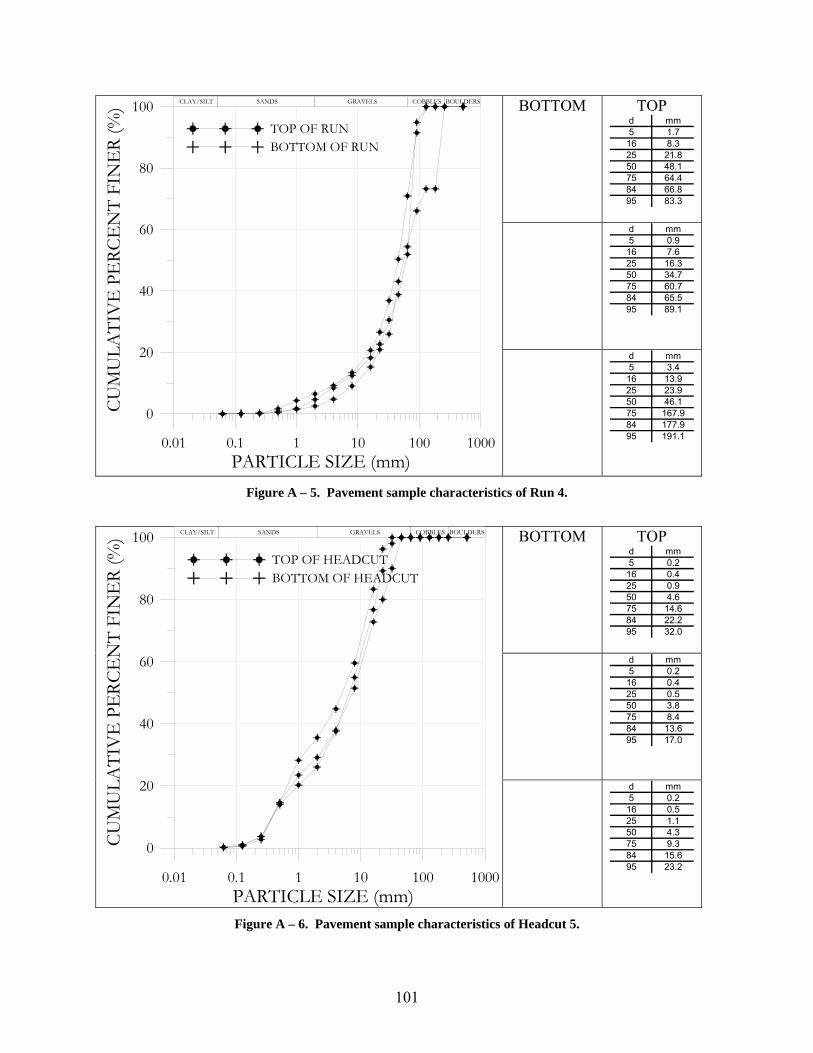
101

BOTTOM

TOP d mm5 1.716 8.325 21.850 48.175 64.484 66.895 83.3

d mm5 0.916 7.625 16.350 34.775 60.784 65.595 89.1

0.01 0.1 1 10 100 1000PARTICLE SIZE (mm)

0

20

40

60

80

100CU

MU

LATI

VE

PE

RCE

NT

FIN

ER

(%)

TOP OF RUNBOTTOM OF RUN

CLAY/SILT SANDS GRAVELS COBBLES BOULDERS

d mm5 3.416 13.925 23.950 46.175 167.984 177.995 191.1

Figure A – 5. Pavement sample characteristics of Run 4.

BOTTOM

TOP

d mm5 0.216 0.425 0.950 4.675 14.684 22.295 32.0

d mm5 0.216 0.425 0.550 3.875 8.484 13.695 17.0

0.01 0.1 1 10 100 1000PARTICLE SIZE (mm)

0

20

40

60

80

100

CUM

ULA

TIV

E P

ERC

EN

T FI

NE

R (%

)

TOP OF HEADCUTBOTTOM OF HEADCUT

CLAY/SILT SANDS GRAVELS COBBLES BOULDERS

d mm5 0.216 0.525 1.150 4.375 9.384 15.695 23.2

Figure A – 6. Pavement sample characteristics of Headcut 5.

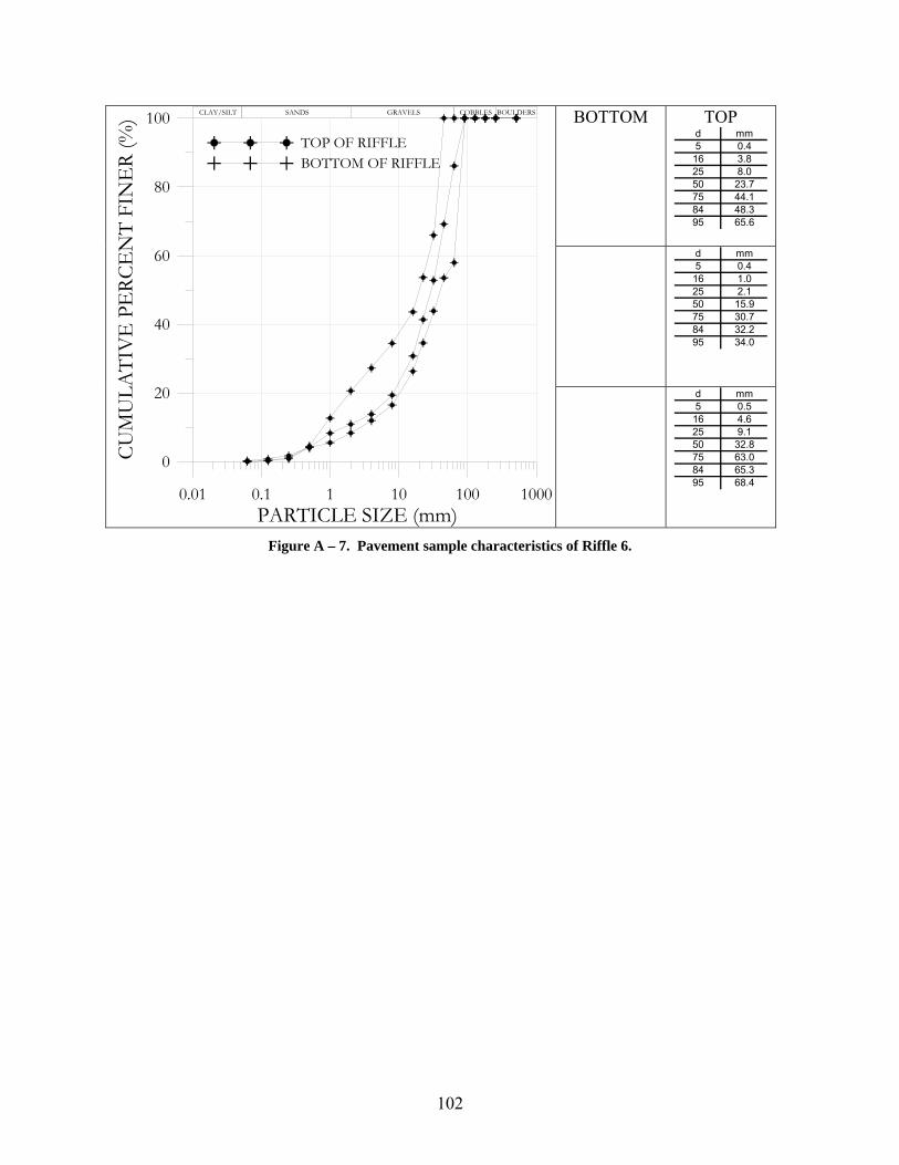
102

BOTTOM

TOP d mm5 0.416 3.825 8.050 23.775 44.184 48.395 65.6

d mm5 0.416 1.025 2.150 15.975 30.784 32.295 34.0

0.01 0.1 1 10 100 1000PARTICLE SIZE (mm)

0

20

40

60

80

100CU

MU

LATI

VE

PE

RCE

NT

FIN

ER

(%)

TOP OF RIFFLEBOTTOM OF RIFFLE

CLAY/SILT SANDS GRAVELS COBBLES BOULDERS

d mm5 0.516 4.625 9.150 32.875 63.084 65.395 68.4

Figure A – 7. Pavement sample characteristics of Riffle 6.

103

DA

M

HE

AD

CU

T

RE

SE

RV

OIR

EX

TEN

T

HE

AD

CU

T

0 2000 4000 6000LONGITUDINAL DISTANCE (m)

0

1

2

3

4

MA

IN C

HA

NN

EL

VE

LOC

ITY

(m/s

)

0

1

2

3

4

AV

ER

AG

E C

HA

NN

EL

VE

LOC

ITY

(m/s

)

0

100

200

300

UN

IT S

TREA

M P

OW

ER (W

/m2 )

BANKFULLAVERAGE

b)

a)

c)

Figure A – 8. Results of a) unit stream power, b) average velocity, and c) main channel velocity for

incremental discharge analyses between 0 < Q < Q100, along the longitudinal profile for Big Creek at Delhi.

104

DA

M

HE

AD

CU

T

RE

SE

RV

OIR

EX

TEN

T

HE

AD

CU

T

0 2000 4000 6000LONGITUDINAL PROFILE (m)

0

40

80

120

MA

IN C

HA

NN

EL

SH

EA

R (N

/m2 )

0

20

40

60

80

100

AV

ER

AG

E C

HA

NN

EL

SH

EA

R (N

/m2 )

BANKFULLAVERAGE

b)

a)

Figure A – 9. Results of a) average channel shear stress and b) main channel shear stress for

incremental discharge analyses ranging between Q < Q < Q100 along the longitudinal profile for Big Creek at Delhi .

105

Appendix B: Hawkesville Dam on Conestoga River at Hawkesville Dam Location: Northing: 4823911m Easting: 529356m (Coordinate System: NAD 1983 UTM Zone 17N)

")

UPPERMOST HEADCUT

HAWKESVILLE

HE

RR

GO

TT

TEM

PER

AN

CE

GEDDES

BROADWAY

HAWK

LAWSON

BRICK SCHOOLM

AR

THA DIE

FEN

BA

CH

ER

TEMPERANCE

BROADWAY

0 10.5km

­Legend

") Dam LocationSurvey PointsReservoir Area

FLOW

DAM LOCATION

Figure B – 1. Hawkesville Dam on Conestoga River at Hawkesville site survey.

106

")

!

")

")

UPPERMOST HEADCUT

HAWKESVILLE

HER

RG

OTT

TEM

PER

ANC

E

GEDDES

BROADWAY

HAWK

LAWSON

BRICK SCHOOL

MAR

THA DIE

FEN

BAC

HER

TEMPERANCE

BROADWAY

Riffle 1

Headcut 3

Headcut 2

0 10.5km

­Legend

") Dam Location") Headcut! Riffle / Run

Reservoir AreaFLOW

DAM LOCATION

Figure B – 2. Locations of pavement samples on Conestoga River.at Hawkesville.

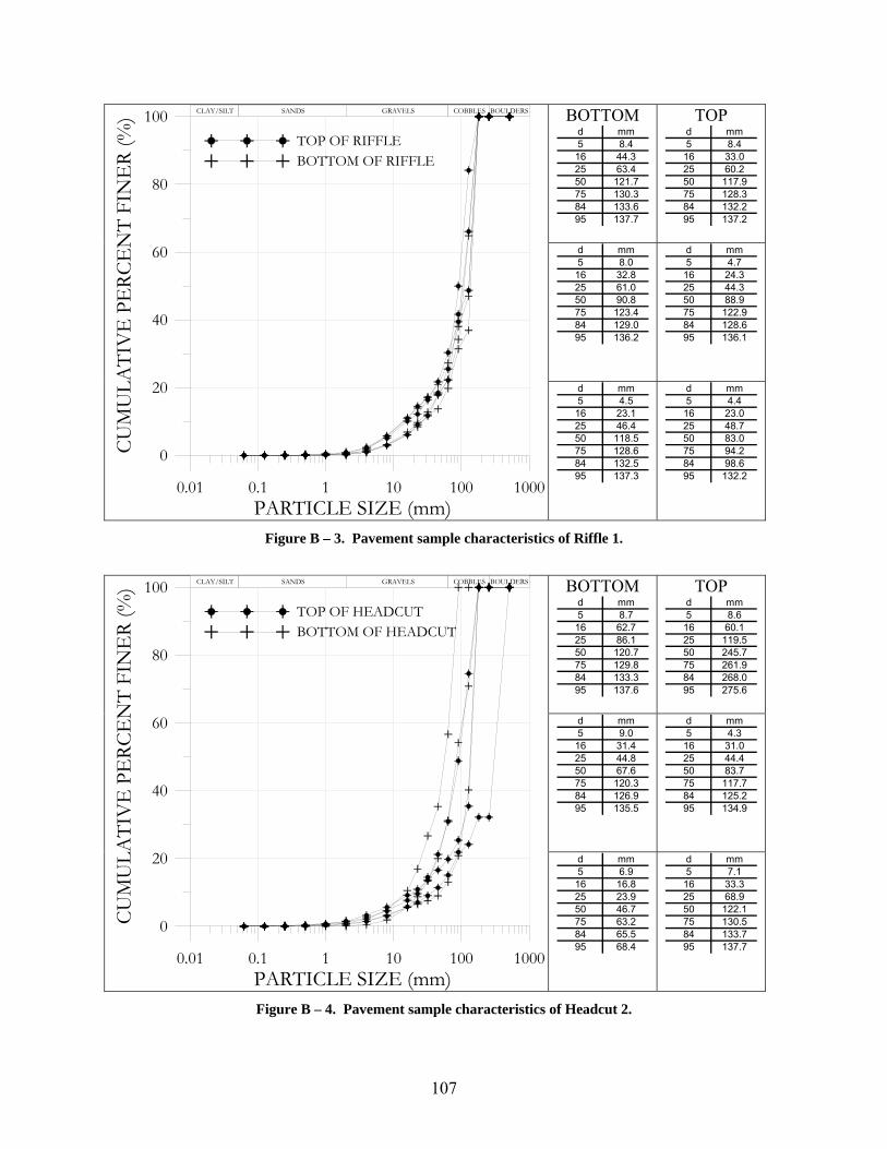
107

BOTTOM d mm5 8.416 44.325 63.450 121.775 130.384 133.695 137.7

TOP d mm5 8.416 33.025 60.250 117.975 128.384 132.295 137.2

d mm5 8.016 32.825 61.050 90.875 123.484 129.095 136.2

d mm5 4.716 24.325 44.350 88.975 122.984 128.695 136.1

0.01 0.1 1 10 100 1000PARTICLE SIZE (mm)

0

20

40

60

80

100CU

MU

LATI

VE

PE

RCE

NT

FIN

ER

(%)

TOP OF RIFFLEBOTTOM OF RIFFLE

CLAY/SILT SANDS GRAVELS COBBLES BOULDERS

d mm5 4.516 23.125 46.450 118.575 128.684 132.595 137.3

d mm5 4.416 23.025 48.750 83.075 94.284 98.695 132.2

Figure B – 3. Pavement sample characteristics of Riffle 1.

BOTTOM

d mm5 8.716 62.725 86.150 120.775 129.884 133.395 137.6

TOP d mm5 8.616 60.125 119.550 245.775 261.984 268.095 275.6

d mm5 9.016 31.425 44.850 67.675 120.384 126.995 135.5

d mm5 4.316 31.025 44.450 83.775 117.784 125.295 134.9

0.01 0.1 1 10 100 1000PARTICLE SIZE (mm)

0

20

40

60

80

100

CUM

ULA

TIV

E P

ERC

EN

T FI

NE

R (%

)

TOP OF HEADCUTBOTTOM OF HEADCUT

CLAY/SILT SANDS GRAVELS COBBLES BOULDERS

d mm5 6.916 16.825 23.950 46.775 63.284 65.595 68.4

d mm5 7.116 33.325 68.950 122.175 130.584 133.795 137.7

Figure B – 4. Pavement sample characteristics of Headcut 2.

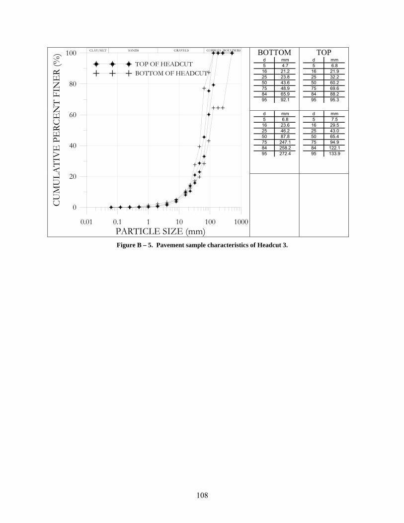
108

BOTTOM d mm5 4.716 21.225 23.850 43.675 48.984 65.995 92.1

TOP d mm5 6.816 21.925 32.250 60.275 69.684 88.295 95.3

d mm5 6.816 23.625 46.250 87.875 247.184 258.295 272.4

d mm5 7.516 29.525 43.050 65.475 94.984 122.195 133.9

0.01 0.1 1 10 100 1000PARTICLE SIZE (mm)

0

20

40

60

80

100CU

MU

LATI

VE

PE

RCE

NT

FIN

ER

(%)

TOP OF HEADCUTBOTTOM OF HEADCUT

CLAY/SILT SANDS GRAVELS COBBLES BOULDERS

Figure B – 5. Pavement sample characteristics of Headcut 3.

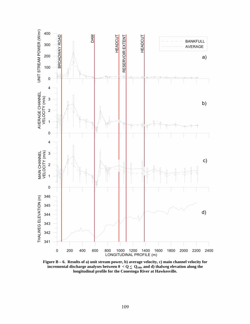
109

0 200 400 600 800 1000 1200 1400 1600 1800 2000 2200 2400LONGITUDINAL PROFILE (m)

341

342

343

344

345

346

THA

LWE

G E

LEV

ATI

ON

(m)

DAM

HE

AD

CU

T

RE

SE

RV

OIR

EX

TEN

T

HE

AD

CU

T

BR

OA

DW

AY

RO

AD

0

1

2

3

4

MA

IN C

HA

NN

EL

VE

LOC

ITY

(m/s

)

0

1

2

3

4

AV

ER

AG

E C

HA

NN

EL

VE

LOC

ITY

(m/s

)

0

100

200

300

400U

NIT

STR

EA

M P

OW

ER

(W/m

2 )BANKFULLAVERAGE

b)

a)

c)

d)

Figure B – 6. Results of a) unit stream power, b) average velocity, c) main channel velocity for

incremental discharge analyses between 0 < Q < Q100, and d) thalweg elevation along the longitudinal profile for the Conestoga River at Hawkesville.

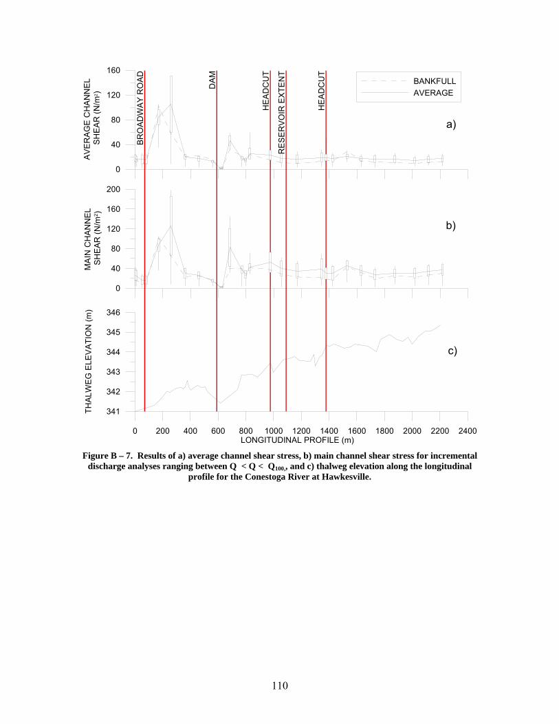
110

0 200 400 600 800 1000 1200 1400 1600 1800 2000 2200 2400LONGITUDINAL PROFILE (m)

341

342

343

344

345

346

THA

LWE

G E

LEV

ATI

ON

(m)

DA

M

HE

AD

CU

T

RE

SE

RV

OIR

EX

TEN

T

HE

AD

CU

T

BR

OA

DW

AY

RO

AD

0

40

80

120

160

200

MA

IN C

HA

NN

EL

SH

EA

R (N

/m2 )

0

40

80

120

160

AV

ER

AG

E C

HA

NN

EL

SH

EA

R (N

/m2 )

BANKFULLAVERAGE

b)

a)

c)

Figure B – 7. Results of a) average channel shear stress, b) main channel shear stress for incremental

discharge analyses ranging between Q < Q < Q100,, and c) thalweg elevation along the longitudinal profile for the Conestoga River at Hawkesville.

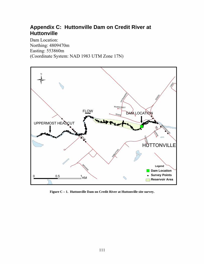
111

Appendix C: Huttonville Dam on Credit River at Huttonville Dam Location: Northing: 4809470m Easting: 553860m (Coordinate System: NAD 1983 UTM Zone 17N)

")UPPERMOST HEADCUT

FLOW DAM LOCATION

HERITAGE

MISSISSAUGA

EMBLETO

N

RIVER

QUEEN

BROWNS

OSTR

ANDE

R

LINKS

CLIFFSID

E

MILL

HURON

RIVERCREST

0 10.5 KM

­

Legend

") Dam LocationSurvey PointsReservoir Area

HUTTONVILLE

Figure C – 1. Huttonville Dam on Credit River at Huttonville site survey.

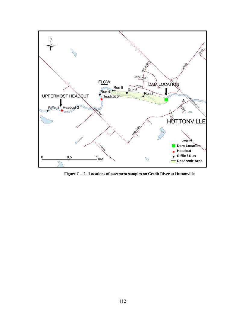
112

")

!

!

!!

!

"

"

UPPERMOST HEADCUT

FLOW DAM LOCATION

HERITAGE

MISSISSAUGA

EMBLE

TON

RIVER

QUEEN

BROWNS

OSTR

ANDE

R

LINKS

CLIFFSID

E

MILL

HURON

RIVERCREST

Run 7Run 6Run 5

Run 4

Riffle 1

Headcut 3

Headcut 2

0 10.5 KM

­

Legend

") Dam Location" Headcut! Riffle / Run

Reservoir Area

HUTTONVILLE

Figure C – 2. Locations of pavement samples on Credit River at Huttonville.

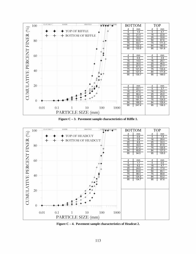
113

BOTTOM d mm5 1.016 21.425 33.250 63.675 93.784 122.295 133.9

TOP d mm5 4.716 22.825 33.850 67.675 171.384 180.395 191.9

d mm5 0.916 14.025 30.550 67.075 121.084 127.495 135.7

d mm5 3.916 29.725 46.550 91.775 133.484 171.995 189.0

0.01 0.1 1 10 100 1000PARTICLE SIZE (mm)

0

20

40

60

80

100CU

MU

LATI

VE

PE

RCE

NT

FIN

ER

(%)

TOP OF RIFFLEBOTTOM OF RIFFLE

CLAY/SILT SANDS GRAVELS COBBLES BOULDERS

d mm5 22.116 47.525 66.450 132.975 181.784 189.595 247.4

d mm5 3.716 24.325 45.050 67.875 124.084 129.495 136.3

Figure C – 3. Pavement sample characteristics of Riffle 1.

BOTTOM

d mm5 0.916 3.925 8.950 34.575 67.284 85.895 94.5

TOP d mm5 7.816 29.425 33.350 61.975 120.584 127.095 135.5

d mm5 1.716 9.225 24.050 83.875 98.384 124.595 134.7

d mm5 0.516 4.725 17.050 65.175 89.884 93.295 97.6

0.01 0.1 1 10 100 1000PARTICLE SIZE (mm)

0

20

40

60

80

100

CUM

ULA

TIV

E P

ERC

EN

T FI

NE

R (%

)

TOP OF HEADCUTBOTTOM OF HEADCUT

CLAY/SILT SANDS GRAVELS COBBLES BOULDERS

Figure C – 4. Pavement sample characteristics of Headcut 2.

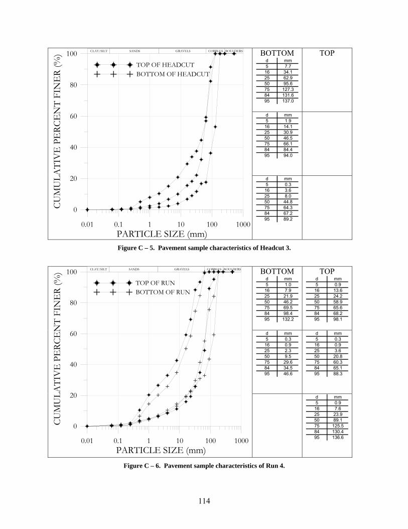
114

BOTTOM d mm5 7.716 34.125 62.950 95.675 127.384 131.695 137.0

TOP

d mm5 1.916 14.125 30.950 46.575 66.184 84.495 94.0

0.01 0.1 1 10 100 1000PARTICLE SIZE (mm)

0

20

40

60

80

100CU

MU

LATI

VE

PE

RCE

NT

FIN

ER

(%)

TOP OF HEADCUTBOTTOM OF HEADCUT

CLAY/SILT SANDS GRAVELS COBBLES BOULDERS

d mm5 0.316 3.625 8.050 44.875 64.384 67.295 89.2

Figure C – 5. Pavement sample characteristics of Headcut 3.

BOTTOM

d mm5 1.016 7.925 21.950 46.275 69.584 98.495 132.2

TOP d mm5 0.916 13.625 24.250 58.975 65.684 68.295 98.1

d mm5 0.316 0.925 2.350 9.575 29.684 34.595 46.6

d mm5 0.316 0.925 3.650 20.875 60.384 65.195 88.3

0.01 0.1 1 10 100 1000PARTICLE SIZE (mm)

0

20

40

60

80

100

CUM

ULA

TIV

E P

ERC

EN

T FI

NE

R (%

)

TOP OF RUNBOTTOM OF RUN

CLAY/SILT SANDS GRAVELS COBBLES BOULDERS

d mm5 0.916 7.625 23.950 89.175 125.584 130.495 136.6

Figure C – 6. Pavement sample characteristics of Run 4.

115

BOTTOM d mm5 1.016 8.825 30.150 66.175 89.784 92.895 96.8

TOP d mm5 0.916 9.425 30.150 87.475 124.284 129.695 136.4

d mm5 3.416 30.525 45.450 90.875 244.384 256.395 271.8

d mm5 7.116 44.525 84.250 129.675 423.284 439.395 459.9

0.01 0.1 1 10 100 1000PARTICLE SIZE (mm)

0

20

40

60

80

100CU

MU

LATI

VE

PE

RCE

NT

FIN

ER

(%)

TOP OF RUNBOTTOM OF RUN

CLAY/SILT SANDS GRAVELS COBBLES BOULDERS

d mm5 1.216 9.025 22.650 59.775 120.384 126.995 135.5

d mm5 4.416 32.025 48.750 83.875 123.884 129.295 136.3

Figure C – 7. Pavement sample characteristics of Run 5.

BOTTOM

d mm5 0.616 7.125 17.050 61.275 92.184 122.795 134.1

TOP d mm5 1.016 9.125 32.050 86.175 126.184 130.895 136.8

d mm5 0.516 2.325 8.050 32.375 86.284 93.895 128.7

d mm5 0.616 4.625 16.450 62.375 87.984 92.795 119.1

0.01 0.1 1 10 100 1000PARTICLE SIZE (mm)

0

20

40

60

80

100

CUM

ULA

TIV

E P

ERC

EN

T FI

NE

R (%

)

TOP OF RUNBOTTOM OF RUN

CLAY/SILT SANDS GRAVELS COBBLES BOULDERS

d mm5 0.916 8.125 23.750 67.675 183.984 235.595 264.7

d mm5 0.516 2.025 6.850 23.875 48.584 62.495 68.2

Figure C – 8. Pavement sample characteristics of Run 6.

116

BOTTOM

TOP d mm5 1.716 7.925 24.250 62.675 93.184 121.595 133.7

d mm5 0.316 1.825 4.450 22.175 43.484 59.195 90.0

0.01 0.1 1 10 100 1000PARTICLE SIZE (mm)

0

20

40

60

80

100CU

MU

LATI

VE

PE

RCE

NT

FIN

ER

(%)

TOP OF RUNBOTTOM OF RUN

CLAY/SILT SANDS GRAVELS COBBLES BOULDERS

Figure C – 9. Pavement sample characteristics of Run 7.

117

88

90

92

94

96

98

THA

LWE

G E

LEV

ATI

ON

(m)

DA

M

RE

SE

RVO

IR E

XTE

NT

HE

AD

CU

T

HE

AD

CU

T

HE

RIT

AG

E R

OA

D

0 1000 2000 3000LONGITUDINAL PROFILE (m)

0

1

2

3

4

MA

IN C

HA

NN

EL

VEL

OC

ITY

(m/s

)

0

1

2

3

4

AVE

RA

GE

CH

ANN

EL

VE

LOC

ITY

(m/s

)

0

100

200

300

400U

NIT

STR

EA

M P

OW

ER

(W/m

2 )

BANKFULLAVERAGE

a)

b)

c)

d)

Figure C – 10. Results of a) unit stream power, b) average velocity, c) main channel velocity for

incremental discharge analyses between 0 < Q < Q100, and d) thalweg elevation along the longitudinal profile for Credit River at Huttonville.

118

88

90

92

94

96

98

THA

LWE

G E

LEV

ATI

ON

(m)

DA

M

RE

SE

RV

OIR

EX

TEN

T

HE

AD

CU

T

HE

AD

CU

T

HER

ITA

GE

RO

AD

0 1000 2000 3000LONGITUDINAL PROFILE (m)

0

40

80

120

160

MA

IN C

HA

NN

EL

SH

EAR

(N/m

2 )

0

40

80

120

160

AV

ER

AG

E C

HA

NN

EL

SH

EA

R (N

/m2 )

BANKFULLAVERAGE

a)

b)

c)

Figure C – 11. HEC Results of a) average channel shear stress, b) main channel shear stress for

incremental discharge analyses ranging between Q < Q < Q100, and c) thalweg elevation along the longitudinal profile for Credit River at Huttonville.

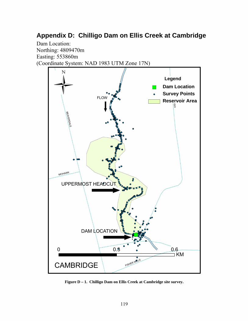
119

Appendix D: Chilligo Dam on Ellis Creek at Cambridge Dam Location: Northing: 4809470m Easting: 553860m (Coordinate System: NAD 1983 UTM Zone 17N)

")

CH

ILLIGO

BEAVERD

ALE

FISHER MILLS

MOHAWK

0 0.60.3KM

­ Legend

") Dam LocationSurvey PointsReservoir Area

CAMBRIDGE

UPPERMOST HEADCUT

FLOW

DAM LOCATION

Figure D – 1. Chilligo Dam on Ellis Creek at Cambridge site survey.

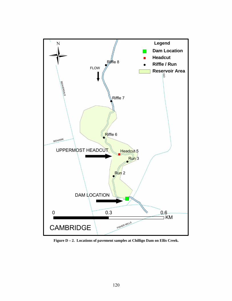
120

")

!

!

!

!

!

")

CH

ILLIGO

BEAVERD

ALE

FISHER MILLS

MOHAWK

Run 3

Run 2

Riffle 6

Riffle 7

Riffle 8

Headcut 5

0 0.60.3KM

­Legend

") Dam Location") Headcut! Riffle / Run

Reservoir Area

CAMBRIDGE

UPPERMOST HEADCUT

FLOW

DAM LOCATION

Figure D – 2. Locations of pavement samples at Chilligo Dam on Ellis Creek.

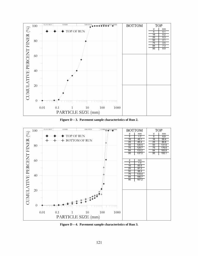
121

BOTTOM

TOP d mm5 0.116 0.225 0.350 2.175 4.584 7.395 8.9

0.01 0.1 1 10 100 1000PARTICLE SIZE (mm)

0

20

40

60

80

100CU

MU

LATI

VE

PE

RCE

NT

FIN

ER

(%)

TOP OF RUN

CLAY/SILT SANDS GRAVELS COBBLES BOULDERS

Figure D – 3. Pavement sample characteristics of Run 2.

BOTTOM

d mm5 1.716 45.125 85.450 120.575 129.784 133.295 137.5

TOP d mm5 6.916 59.425 89.850 131.675 176.684 183.895 193.1

d mm5 1.016 83.525 87.250 98.475 133.484 166.795 187.2

0.01 0.1 1 10 100 1000PARTICLE SIZE (mm)

0

20

40

60

80

100

CUM

ULA

TIV

E P

ERC

EN

T FI

NE

R (%

)

TOP OF RUNBOTTOM OF RUN

CLAY/SILT SANDS GRAVELS COBBLES BOULDERS

Figure D – 4. Pavement sample characteristics of Run 3.

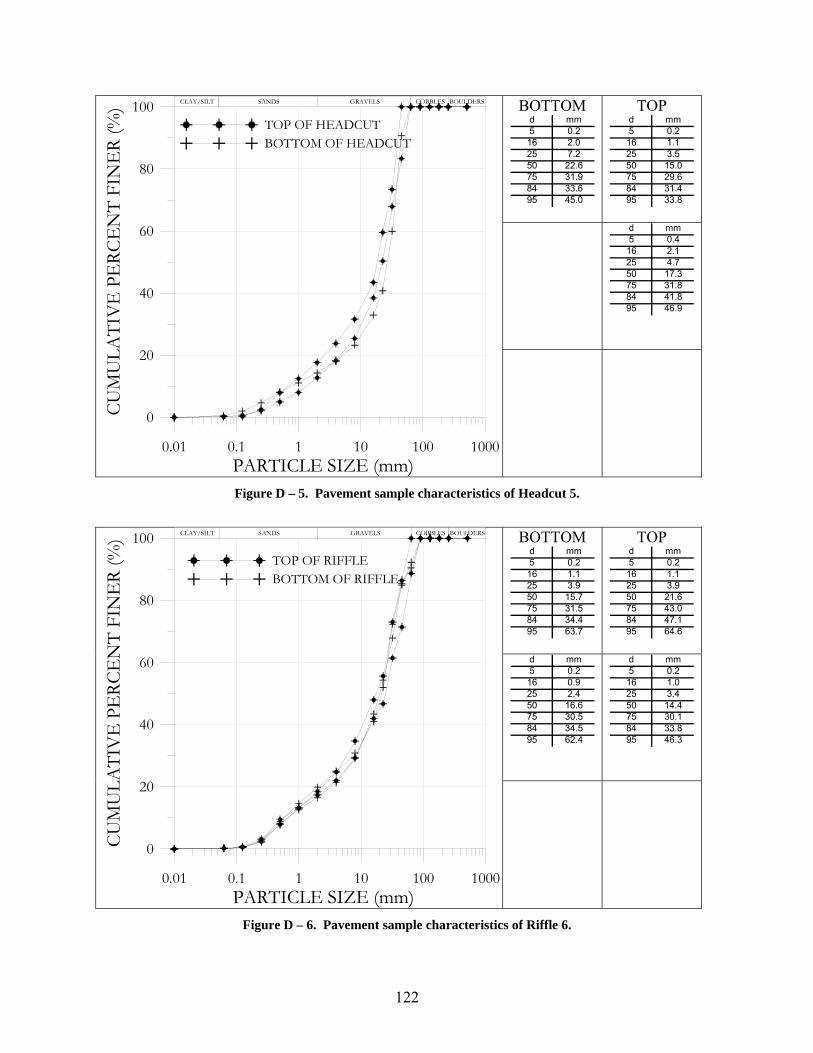
122

BOTTOM d mm5 0.216 2.025 7.250 22.675 31.984 33.695 45.0

TOP d mm5 0.216 1.125 3.550 15.075 29.684 31.495 33.8

d mm5 0.416 2.125 4.750 17.375 31.884 41.895 46.9

0.01 0.1 1 10 100 1000PARTICLE SIZE (mm)

0

20

40

60

80

100CU

MU

LATI

VE

PE

RCE

NT

FIN

ER

(%)

TOP OF HEADCUTBOTTOM OF HEADCUT

CLAY/SILT SANDS GRAVELS COBBLES BOULDERS

Figure D – 5. Pavement sample characteristics of Headcut 5.

BOTTOM

d mm5 0.216 1.125 3.950 15.775 31.584 34.495 63.7

TOP d mm5 0.216 1.125 3.950 21.675 43.084 47.195 64.6

d mm5 0.216 0.925 2.450 16.675 30.584 34.595 62.4

d mm5 0.216 1.025 3.450 14.475 30.184 33.895 46.3

0.01 0.1 1 10 100 1000PARTICLE SIZE (mm)

0

20

40

60

80

100

CUM

ULA

TIV

E P

ERC

EN

T FI

NE

R (%

)

TOP OF RIFFLEBOTTOM OF RIFFLE

CLAY/SILT SANDS GRAVELS COBBLES BOULDERS

Figure D – 6. Pavement sample characteristics of Riffle 6.

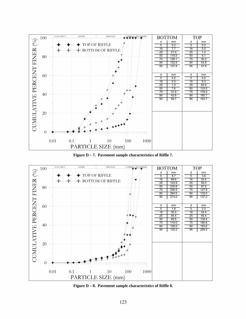
123

BOTTOM

d mm5 0.316 7.725 21.050 119.575 129.184 132.895 137.4

TOP d mm5 0.216 0.525 1.250 9.175 30.284 43.895 47.6

d mm5 0.216 0.525 1.050 7.675 31.984 42.695 59.7

d mm5 0.516 9.325 63.550 133.075 179.484 185.795 193.7

0.01 0.1 1 10 100 1000PARTICLE SIZE (mm)

0

20

40

60

80

100CU

MU

LATI

VE

PE

RCE

NT

FIN

ER

(%)

TOP OF RIFFLEBOTTOM OF RIFFLE

CLAY/SILT SANDS GRAVELS COBBLES BOULDERS

Figure D – 7. Pavement sample characteristics of Riffle 7.

BOTTOM

d mm5 8.716 89.625 123.950 235.875 256.584 264.595 274.5

TOP d mm5 3.616 33.425 59.050 97.575 127.984 132.095 137.2

d mm5 1.816 30.325 44.450 69.575 119.084 126.095 135.2

d mm5 2.316 34.425 65.450 139.475 185.884 193.695 259.3

0.01 0.1 1 10 100 1000PARTICLE SIZE (mm)

0

20

40

60

80

100

CUM

ULA

TIV

E P

ERC

EN

T FI

NE

R (%

)

TOP OF RIFFLEBOTTOM OF RIFFLE

CLAY/SILT SANDS GRAVELS COBBLES BOULDERS

Figure D – 8. Pavement sample characteristics of Riffle 8.

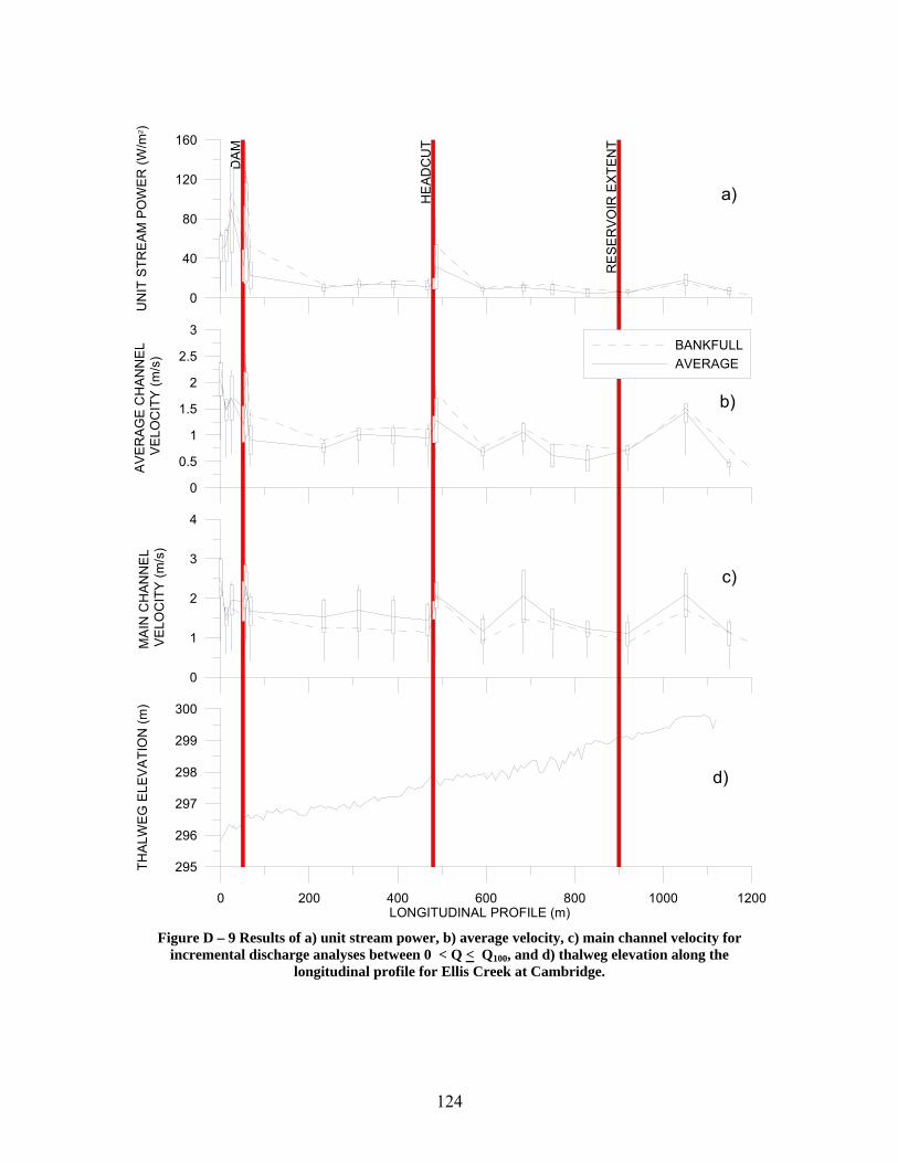
124

0 200 400 600 800 1000 1200LONGITUDINAL PROFILE (m)

295

296

297

298

299

300

THA

LWEG

ELE

VA

TIO

N (m

)

DA

M

HE

ADC

UT

RE

SER

VO

IR E

XTEN

T

0

1

2

3

4

MA

IN C

HAN

NE

L V

ELO

CIT

Y (m

/s)

0

0.5

1

1.5

2

2.5

3

AVE

RA

GE

CH

AN

NEL

VE

LOC

ITY

(m/s

)

0

40

80

120

160U

NIT

STR

EA

M P

OW

ER (W

/m2 )

BANKFULLAVERAGE

a)

b)

c)

d)

Figure D – 9 Results of a) unit stream power, b) average velocity, c) main channel velocity for

incremental discharge analyses between 0 < Q < Q100, and d) thalweg elevation along the longitudinal profile for Ellis Creek at Cambridge.

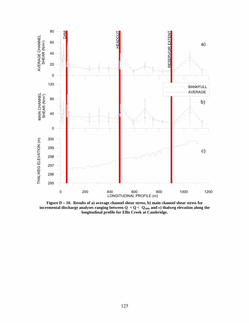
125

0 200 400 600 800 1000 1200LONGITUDINAL PROFILE (m)

295

296

297

298

299

300

THA

LWE

G E

LEV

ATI

ON

(m)

DAM

HE

AD

CU

T

RE

SE

RV

OIR

EXT

EN

T

0

40

80

120

MA

IN C

HA

NN

EL

SH

EAR

(N/m

2 )

0

20

40

60

80

AV

ER

AG

E C

HA

NN

EL

SH

EA

R (N

/m2 )

BANKFULLAVERAGE

a)

b)

c)

Figure D – 10. Results of a) average channel shear stress, b) main channel shear stress for

incremental discharge analyses ranging between Q < Q < Q100, and c) thalweg elevation along the longitudinal profile for Ellis Creek at Cambridge.

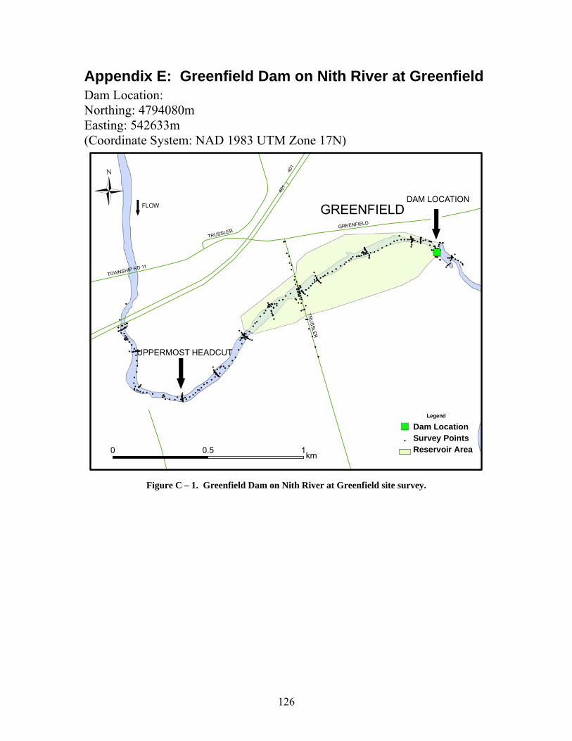
126

Appendix E: Greenfield Dam on Nith River at Greenfield Dam Location: Northing: 4794080m Easting: 542633m (Coordinate System: NAD 1983 UTM Zone 17N)

%

%%%%%%%%%%%%%%

%%

%%

%%% %

%%%%

%%%

%%% %%%%

%

%%%

%

%%%

%

%%%%%%%%%%%

%%

%

%%%%%%%%%%%%

%%%%%

%%%%%%%%%%%%%

%

%%%%%%%%%%

%%%%%%%%%%%%%%%%

%

% %%%%%%

%%

%%

%%

%%% %

%

%%%%%%

%%

%%

%%

%

%

%

%

%

%

%

%

%

%

%

%

% %

%

%

%

%%%%

%%%%%%

%

%

%%

%

%

%

%

%

%

%%%%

%%%%%%

%%

%%

%

%

%%%%

%%%

%

%

%

%

%

%

%

%

%

%

%

%

%%

%

%%%

%%

%%%

%%%%

%%%

%

%%%

%%%

%

%

%%

%

%%

%

%

%

%

%%

%

%

%

%

%

%

%

%

%

%

%%

%

%

%

%%

$

$$$

$$$$

$$$$$

$ $

$$

$$$$

$$$$$

$$

$$$$$

$

$

$$$$

$

$

$

$$

$

$$

$$$

$$

$$$$$$$$$$$$$$$$$$

$$$

$

$

$

$

$$$$

$

$

$

$

$

$$$

$

$$$$$

$$$$

$

$

$

$$

$$$

$$

$$

$

$

$ $$$$$

$$$$

$

$$$

$$$$

$$$$$$

$$

$

$$$$ $ $

$$

$$$$

$

$

$

$

$

$

$

$$

$

$

$

$

$$$

$$$$

$$

$$$$$$$ $$$

$$

$$$

$$$

$$

$$$$$$$$$$$$

$

$

")

UPPERMOST HEADCUT

GREENFIELDDAM LOCATION

401

TRU

SSLER

GREENFIELD

TOWNSHIP RD 11

401

TRUSSLER

0 10.5 km

­

Legend

") Dam Location$ Survey Points

Reservoir Area

FLOW

Figure C – 1. Greenfield Dam on Nith River at Greenfield site survey.

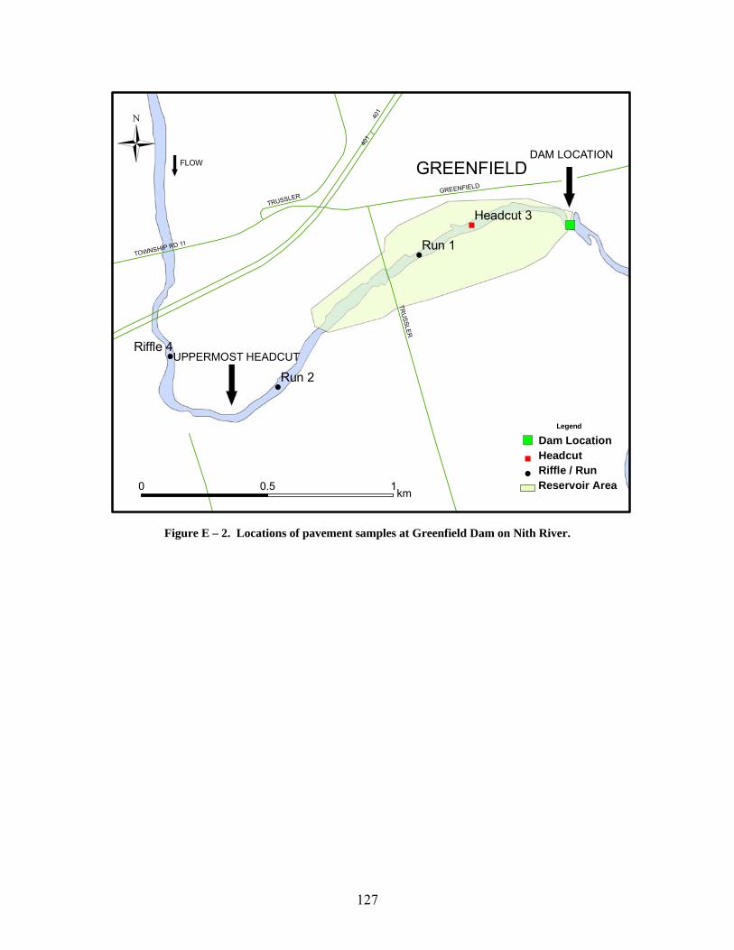
127

")

!

!

!

"

UPPERMOST HEADCUT

GREENFIELDDAM LOCATION

401

TRU

SSLER

GREENFIELD

TOWNSHIP RD 11

401

TRUSSLER

Run 1

Run 2

Riffle 4

Headcut 3

0 10.5 km

­

Legend

") Dam Location" Headcut! Riffle / Run

Reservoir Area

FLOW

Figure E – 2. Locations of pavement samples at Greenfield Dam on Nith River.

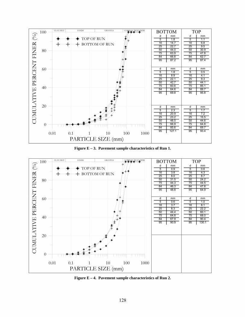
128

BOTTOM d mm5 1.816 14.725 22.750 44.075 63.984 66.895 87.2

TOP d mm5 1.116 6.825 9.550 30.975 47.884 62.795 87.4

d mm5 1.816 8.925 22.150 42.775 60.684 64.695 69.8

d mm5 0.516 4.125 9.350 44.175 85.184 89.795 95.8

0.01 0.1 1 10 100 1000PARTICLE SIZE (mm)

0

20

40

60

80

100CU

MU

LATI

VE

PE

RCE

NT

FIN

ER

(%)

TOP OF RUNBOTTOM OF RUN

CLAY/SILT SANDS GRAVELS COBBLES BOULDERS

d mm5 2.316 20.925 23.250 48.575 66.984 85.695 127.1

d mm5 1.716 7.225 15.550 44.675 64.884 69.795 93.4

Figure E – 3. Pavement sample characteristics of Run 1.

BOTTOM

d mm5 0.916 3.825 8.050 31.575 44.384 46.395 48.8

TOP d mm5 0.616 4.325 8.750 24.275 44.584 47.895 64.9

d mm5 0.616 3.725 8.350 44.475 64.884 67.995 90.9

d mm5 1.016 8.125 22.250 60.175 68.084 90.495 130.1

0.01 0.1 1 10 100 1000PARTICLE SIZE (mm)

0

20

40

60

80

100

CUM

ULA

TIV

E P

ERC

EN

T FI

NE

R (%

)

TOP OF RUNBOTTOM OF RUN

CLAY/SILT SANDS GRAVELS COBBLES BOULDERS

Figure E – 4. Pavement sample characteristics of Run 2.

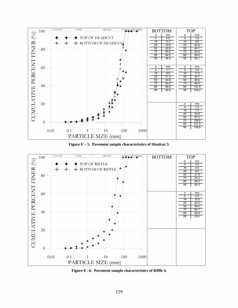
129

BOTTOM d mm5 2.216 13.725 22.950 42.675 65.284 84.595 94.0

TOP d mm5 1.016 8.925 22.250 44.175 62.884 69.095 93.1

d mm5 1.116 8.825 21.450 44.875 65.084 68.895 92.6

d mm5 3.916 17.225 30.150 65.675 95.884 122.495 134.0

0.01 0.1 1 10 100 1000PARTICLE SIZE (mm)

0

20

40

60

80

100CU

MU

LATI

VE

PE

RCE

NT

FIN

ER

(%)

TOP OF HEADCUTBOTTOM OF HEADCUT

CLAY/SILT SANDS GRAVELS COBBLES BOULDERS

d mm5 1.216 7.425 20.950 87.275 126.884 131.395 136.9

Figure E – 5. Pavement sample characteristics of Headcut 3.

BOTTOM

TOP

d mm5 0.316 4.025 8.050 21.975 34.384 46.495 65.0

d mm5 2.216 14.025 23.450 46.075 84.784 92.995 128.1

0.01 0.1 1 10 100 1000PARTICLE SIZE (mm)

0

20

40

60

80

100

CUM

ULA

TIV

E P

ERC

EN

T FI

NE

R (%

)

TOP OF RIFFLEBOTTOM OF RIFFLE

CLAY/SILT SANDS GRAVELS COBBLES BOULDERS

Figure E –6. Pavement sample characteristics of Riffle 4.

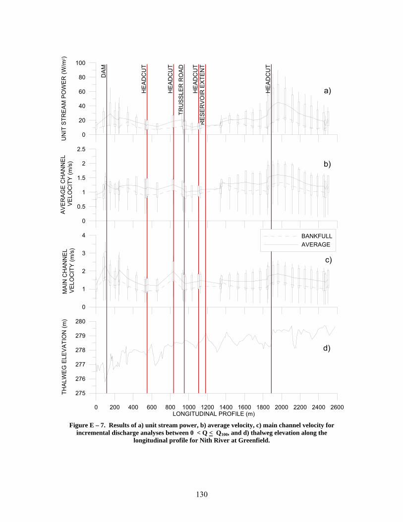
130

0 200 400 600 800 1000 1200 1400 1600 1800 2000 2200 2400 2600LONGITUDINAL PROFILE (m)

275

276

277

278

279

280

THA

LWEG

ELE

VATI

ON

(m)

DA

M

HE

AD

CU

T

HE

AD

CU

T

HE

AD

CU

TR

ES

ER

VO

IR E

XTE

NT

HE

AD

CU

T

TRU

SS

LER

RO

AD

0

1

2

3

4

MA

IN C

HA

NN

EL

VEL

OC

ITY

(m/s

)

0

0.5

1

1.5

2

2.5

AV

ER

AG

E C

HAN

NE

L V

ELO

CIT

Y (m

/s)

0

20

40

60

80

100U

NIT

STR

EA

M P

OW

ER

(W/m

2 )

BANKFULLAVERAGE

b)

a)

c)

d)

Figure E – 7. Results of a) unit stream power, b) average velocity, c) main channel velocity for

incremental discharge analyses between 0 < Q < Q100, and d) thalweg elevation along the longitudinal profile for Nith River at Greenfield.

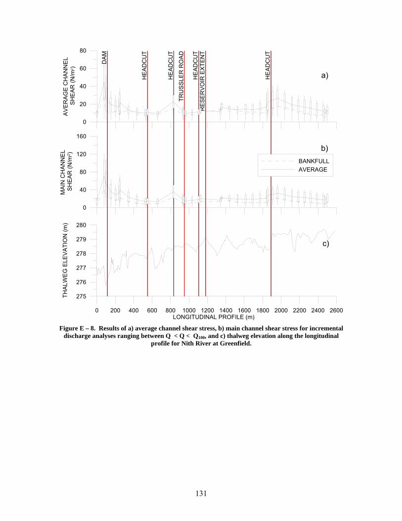
131

0 200 400 600 800 1000 1200 1400 1600 1800 2000 2200 2400 2600LONGITUDINAL PROFILE (m)

275

276

277

278

279

280

THA

LWE

G E

LEV

ATI

ON

(m)

DA

M

HE

AD

CU

T

HE

AD

CU

T

HE

AD

CU

TR

ES

ER

VO

IR E

XTE

NT

HE

AD

CU

T

TRU

SS

LER

RO

AD

0

40

80

120

160

MA

IN C

HA

NN

EL

SH

EA

R (N

/m2 )

0

20

40

60

80

AV

ER

AG

E C

HA

NN

EL

SH

EA

R (N

/m2 )

BANKFULLAVERAGE

b)

a)

c)

Figure E – 8. Results of a) average channel shear stress, b) main channel shear stress for incremental

discharge analyses ranging between Q < Q < Q100, and c) thalweg elevation along the longitudinal profile for Nith River at Greenfield.

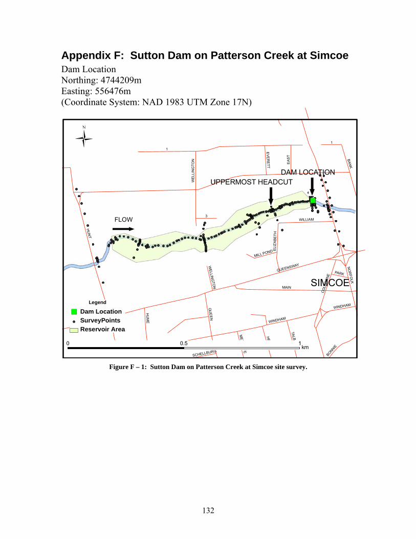
132

Appendix F: Sutton Dam on Patterson Creek at Simcoe Dam Location Northing: 4744209m Easting: 556476m (Coordinate System: NAD 1983 UTM Zone 17N)

")

2

1

HU

NT

QUEENSWAY

MAIN

NO

RFO

LK

3

WINDHAM

BANK

QU

EEN

CO

LBO

RN

E

WILLIAM

HU

ME

HEAD

WEL

LIN

GTO

N

EAS

T

TALBO

T

BONNIE

ELIZ

ABET

HPARK

EVER

ETT

MILL POND

METC

ALFE

SCHELLBURG

WINDHAM

1

WELLIN

GTO

N

0 10.5km

­

Legend

") Dam LocationSurveyPointsReservoir Area

SIMCOE

UPPERMOST HEADCUT

FLOW

DAM LOCATION

Figure F – 1: Sutton Dam on Patterson Creek at Simcoe site survey.

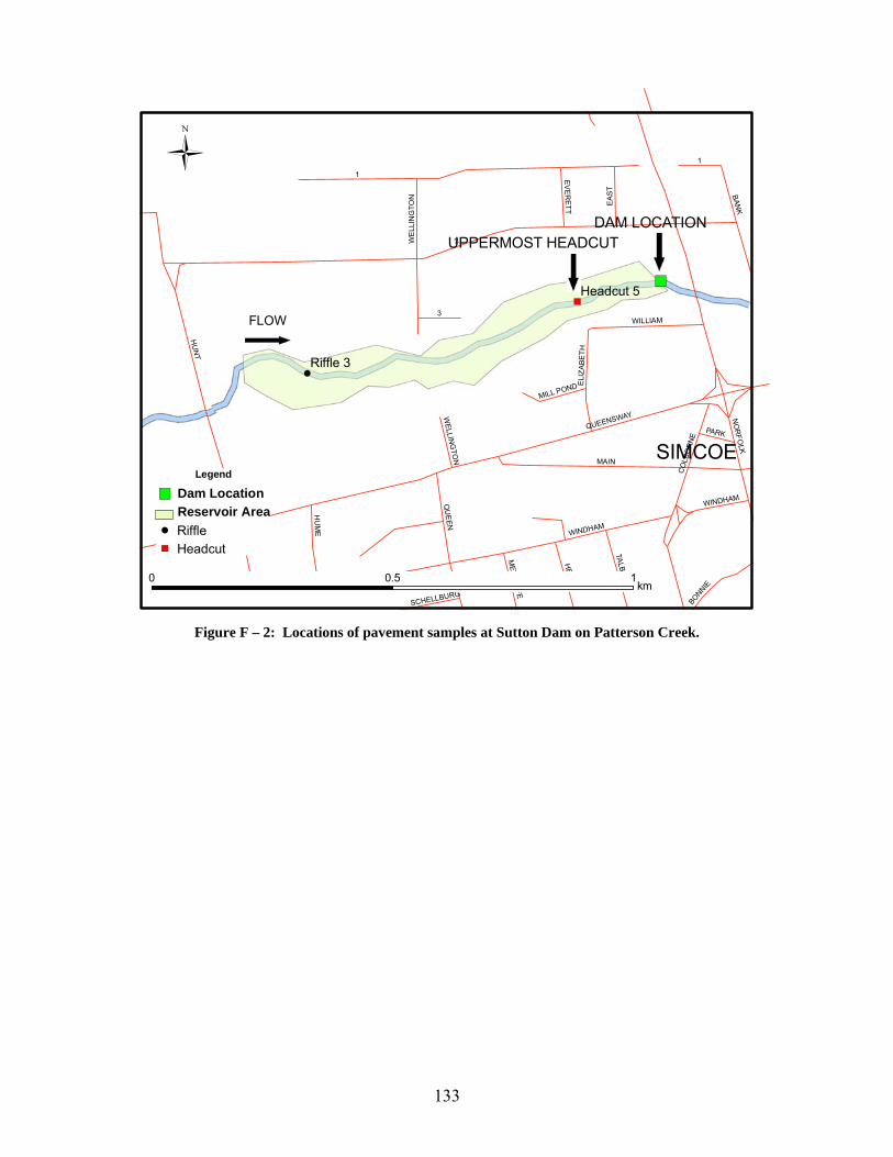
133

")

!

")

2

1

HU

NT

QUEENSWAY

MAIN

NO

RFO

LK

3

WINDHAM

BANK

QU

EEN

CO

LBO

RN

E

WILLIAM

HU

ME

HEAD

WE

LLIN

GTO

N

EAS

T

TALBO

T

BONNIE

ELI

ZABE

T H

PARK

EVER

ETT

MILL PONDM

ETCALFE

SCHELLBURG

WINDHAM

1

WELLIN

GTO

N

Riffle 3

Headcut 5

0 10.5km

­

Legend

") Dam LocationReservoir Area

! Riffle") Headcut

SIMCOE

UPPERMOST HEADCUT

FLOW

DAM LOCATION

Figure F – 2: Locations of pavement samples at Sutton Dam on Patterson Creek.

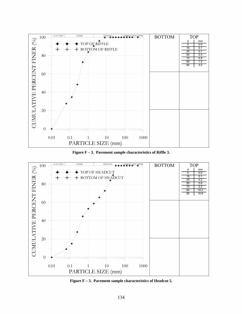
134

BOTTOM

TOP

d mm5 0.016 0.125 0.150 0.375 0.884 1.095 3.0

0.01 0.1 1 10 100 1000PARTICLE SIZE (mm)

0

20

40

60

80

100CU

MU

LATI

VE

PE

RCE

NT

FIN

ER

(%)

TOP OF RIFFLEBOTTOM OF RIFFLE

CLAY/SILT SANDS GRAVELS COBBLES BOULDERS

Figure F – 3. Pavement sample characteristics of Riffle 3.

BOTTOM

TOP

d mm5 0.016 0.125 0.250 0.675 2.284 10.295 10.6

0.01 0.1 1 10 100 1000PARTICLE SIZE (mm)

0

20

40

60

80

100

CUM

ULA

TIV

E P

ERC

EN

T FI

NE

R (%

)

TOP OF HEADCUTBOTTOM OF HEADCUT

CLAY/SILT SANDS GRAVELS COBBLES BOULDERS

Figure F – 3. Pavement sample characteristics of Headcut 5.

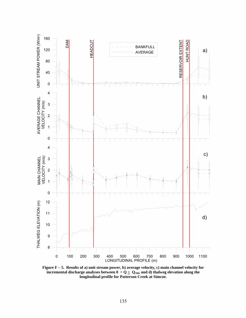
135

0 100 200 300 400 500 600 700 800 900 1000 1100LONGITUDINAL PROFILE (m)

8

9

10

11

12

THAL

WEG

ELE

VATI

ON

(m)

DA

M

HE

AD

CU

T

RE

SE

RV

OIR

EX

TEN

T

HU

NT

RO

AD

0

1

2

3

4

MA

IN C

HA

NN

EL

VEL

OC

ITY

(m/s

)

0

1

2

3

4

AV

ER

AG

E C

HAN

NEL

VE

LOC

ITY

(m/s

)

0

40

80

120

160U

NIT

STR

EA

M P

OW

ER

(W/m

2 )

BANKFULLAVERAGE

b)

a)

c)

d)

Figure F – 5. Results of a) unit stream power, b) average velocity, c) main channel velocity for

incremental discharge analyses between 0 < Q < Q100, and d) thalweg elevation along the longitudinal profile for Patterson Creek at Simcoe.

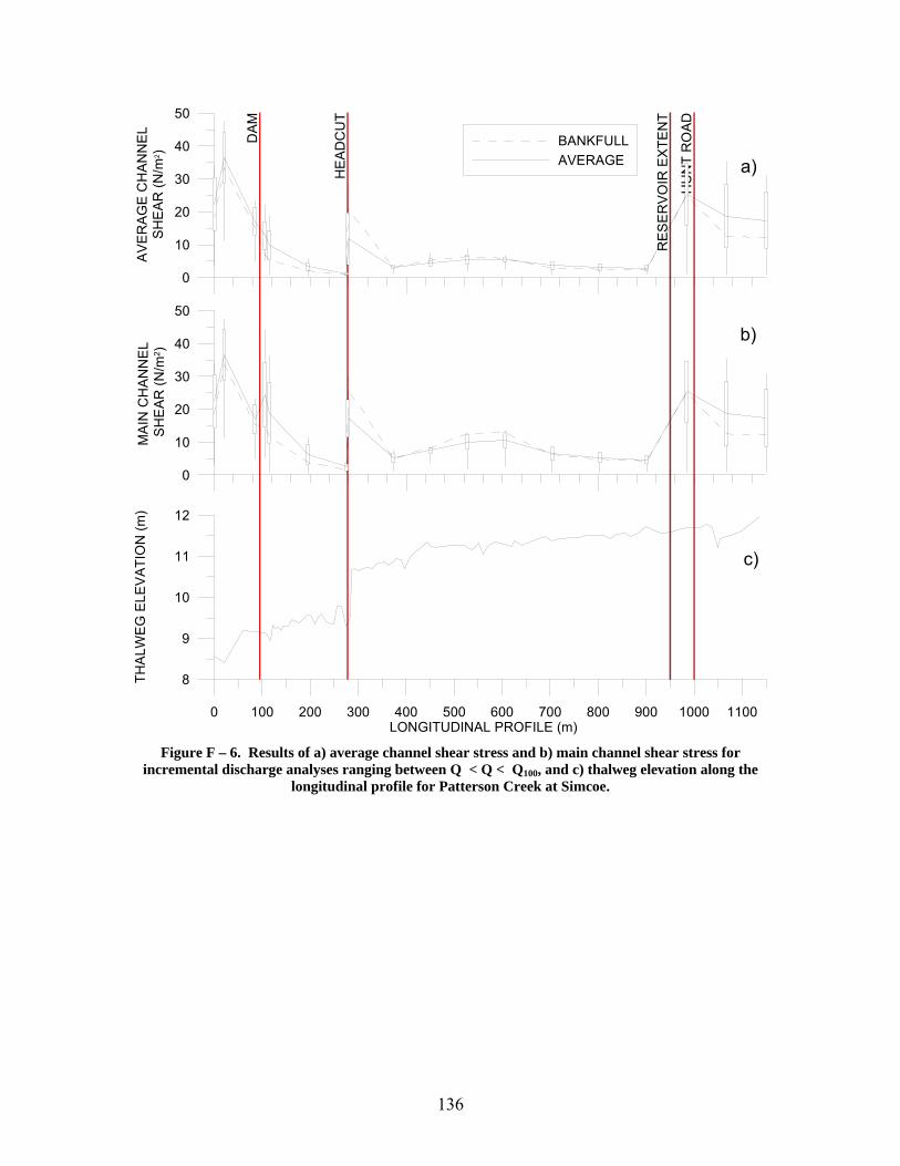
136

0 100 200 300 400 500 600 700 800 900 1000 1100LONGITUDINAL PROFILE (m)

8

9

10

11

12

THA

LWE

G E

LEV

ATI

ON

(m)

DA

M

HE

AD

CU

T

RE

SE

RV

OIR

EX

TEN

T

HU

NT

RO

AD

0

10

20

30

40

50

MA

IN C

HA

NN

EL

SH

EA

R (N

/m2 )

0

10

20

30

40

50

AV

ER

AG

E C

HA

NN

EL

SH

EA

R (N

/m2 )

BANKFULLAVERAGE

b)

a)

c)

Figure F – 6. Results of a) average channel shear stress and b) main channel shear stress for

incremental discharge analyses ranging between Q < Q < Q100, and c) thalweg elevation along the longitudinal profile for Patterson Creek at Simcoe.

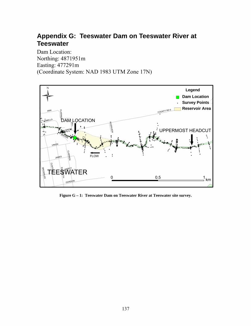
137

Appendix G: Teeswater Dam on Teeswater River at Teeswater Dam Location: Northing: 4871951m Easting: 477291m (Coordinate System: NAD 1983 UTM Zone 17N)

!

!

!

!!

!

!

!

!

! !

!

!

!

!!!

!!!! !! !! !!

!

!

!

!

!

!!

!

!

!

!

!

!

!

!

!

!!

!

!

!

!

!

!

!

!

!

!

!

!

!

!

!

!

!

!

!

!!

!!! !! !

!

!!!!!!!!

!

!

!!!!!!

!

!

!

!

!

!

!!!!!

!

!!!!!

!

!!

!!!!

!!

!!

!!

!!

!!!!!!!!!!

!!!!

!

!!!!

!

!!!!!!!!!!!!!!!!! !!

!

!!!!!!!!!!

!

!!

!

!!!!!!!!!!!!!!!

!

!!!!!!!!!!!!!!

!

!!!! ! !

! ! ! !!! !!!!!!!!!!!!!!

!!!! !!!!!

! !!! ! !

!!!

!

!

!

!!

!

!

!

!

!

!

!

!

!

!

!

!!!!!

! !

!!

!

!

!

!

!

!!

!

!!!!

!

!!!!!

!!!

!!!

!

!

!

!

!

!

!

!

!

!!

!

!!!!!

!

!!!

!

!

!

!!

!

!

!

!

!

!

!!

!

!!!

!

!! !!

!

!

!!

!!!!

!

!

!

!

!

!

!

!

!

!

!

!

!

!

!

!

!!

!

!

!

!!!

!

!!

!!

!

!!!

!!!

!!! !!!

!

!!!

!

!

!!

!

!!

!

!!

!!

!

!

!!!!!!!!

!!!!

!!!!!!

!

!

!

!

!!!

!

!

!

!

!!!!

!

!!!!!!!!!!

!

!

!

!!

!

!

!!!!!!

!

!

!

!

!

!

!

!

!

!

!

!

!

!

!

!!!!

!

!

!

!

!

!

!!!!!!

!

!!!

!

!

!!!!!!

!

!

!

!

!!!!!!

!!

! !

!

!!!!!!!!

!

!!

!!!!!!!

!

!!

!

!

!

!

!

!!

!!!!!!!!!

!

!!!!

!

!

!

!!

!!!!!

!

!

!

!

!

!!

!

!

!

!

!

!

!!

!!

!!

!

! !!!!!! !

!!!!!!!!!!! !!!!!!!!!

!!!!

!!! !!!!!!!!

!

!!

!!!!!

!!

!

!

!!

!

!!

!

!!

!!!!! !!!!!!!

!!! !

!

!!

!

!!!!!!!!!!

!!!!

!!

!

!

!!

!

!! !!!!!

!!

!!!!!

!!

!

!!

! !

!

!

!

!

!

!!!!!!

!

!

!!

!

!

!!!!!!!

!!

!!

! !!

!!!

!

!

!

!

!!!

!

!!!!!!!!

!!!!!!!!!

!

!!!!!! !

!!!!!!!!!!!!!!

!!

!

!

!

!

!

!

!! ! ! ! ! !!!

!!!!!!

!

!!

!

! !!

! ! !!!!

!!!!!!

!

!

!

!!

!

!

!!!!!!

!

!!!!!!!

!!!!!!!!!!

!!! !! ! !!

!!!!! !!!

!

!

!!

!!

! !

!!

!

!

!! !! !! !!!!!!!!!!!!!!!!

!!!

!

!

!

!

!

!

!

!!!!!!!!!!!!!!!!

!

!

!

!

!

!

!

!

!

!

!

!!

!

!

!

!

!

")")")

UPPERMOST HEADCUT

CLIN

TON

COUNTY RD 6

HILLCREST

GORDON

JAMES

MARCY

UNION

CLAR

IND

A

ELIZABETH

ANN

MILL

BRO

WN

LEE

BROWN

ISABELLA

RIVER

VIEW

CLA

RIN

DA

0 10.5 km

­Legend

") Dam Location! Survey Points

Reservoir Area

TEESWATER

FLOW

DAM LOCATION

Figure G – 1: Teeswater Dam on Teeswater River at Teeswater site survey.

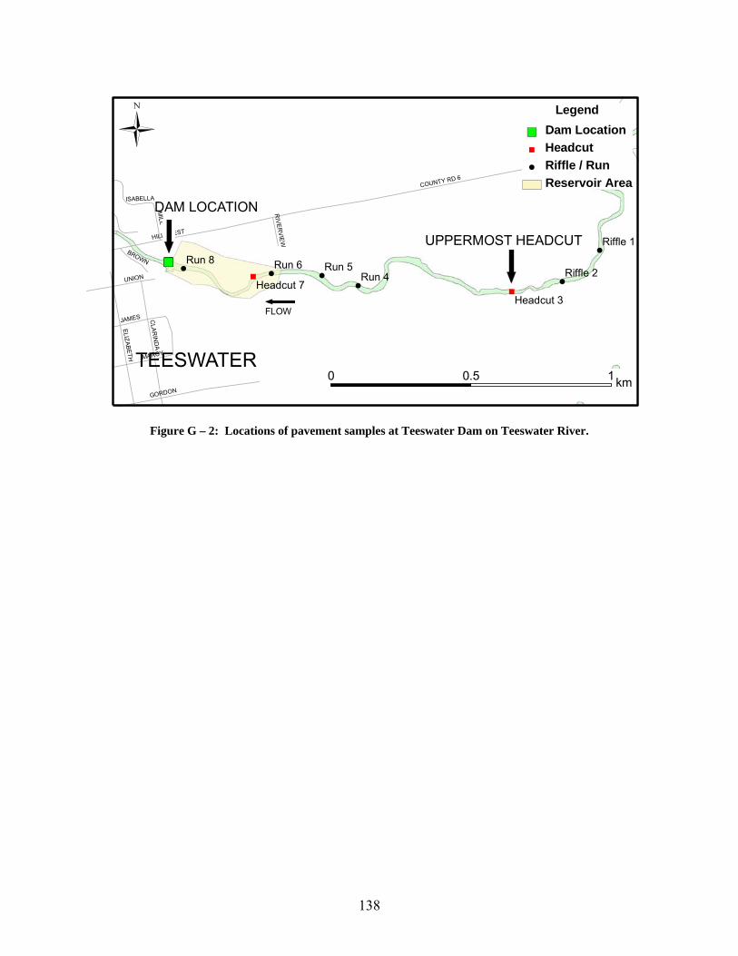
138

")")")

!

!!

!!

!

"

"

UPPERMOST HEADCUT

COUNTY RD 6

HILLCREST

GORDON

CLAR

IND

A

ELIZABETH

MILL

MARCY

JAMES

UNION

SIDEROAD 10

A

BROWN

RIVER

VIEW

ISABELLA

Run 6Run 8 Run 5Run 4 Riffle 2

Riffle 1

Headcut 7Headcut 3

0 10.5 km

­Legend

") Dam Location" Headcut! Riffle / Run

Reservoir Area

TEESWATER

FLOW

DAM LOCATION

Figure G – 2: Locations of pavement samples at Teeswater Dam on Teeswater River.

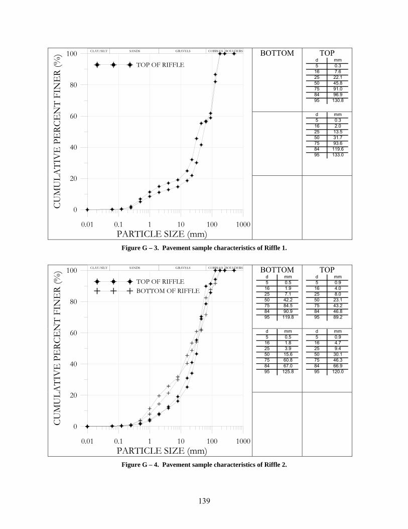
139

BOTTOM

TOP d mm5 0.316 7.625 22.150 45.875 91.084 96.995 130.8

d mm5 0.316 2.025 13.550 31.775 93.684 119.695 133.0

0.01 0.1 1 10 100 1000PARTICLE SIZE (mm)

0

20

40

60

80

100CU

MU

LATI

VE

PE

RCE

NT

FIN

ER

(%)

TOP OF RIFFLE

CLAY/SILT SANDS GRAVELS COBBLES BOULDERS

Figure G – 3. Pavement sample characteristics of Riffle 1.

BOTTOM

d mm5 0.516 1.925 7.150 42.275 84.584 90.995 119.8

TOP d mm5 0.916 4.025 8.050 23.175 43.284 46.895 89.2

d mm5 0.516 1.825 3.950 15.675 60.884 67.095 125.8

d mm5 0.916 4.725 9.450 30.175 46.384 66.995 120.0

0.01 0.1 1 10 100 1000PARTICLE SIZE (mm)

0

20

40

60

80

100

CUM

ULA

TIV

E P

ERC

EN

T FI

NE

R (%

)

TOP OF RIFFLEBOTTOM OF RIFFLE

CLAY/SILT SANDS GRAVELS COBBLES BOULDERS

Figure G – 4. Pavement sample characteristics of Riffle 2.

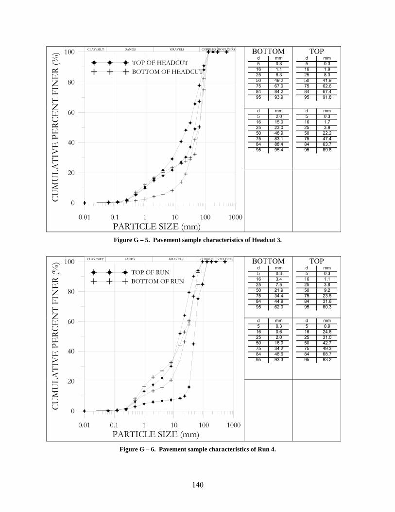
140

BOTTOM d mm5 0.316 1.125 8.350 49.275 67.084 84.295 93.9

TOP d mm5 0.316 1.925 8.350 41.975 62.684 67.495 91.8

d mm5 2.016 15.025 23.050 48.975 83.184 88.495 95.4

d mm5 0.316 1.725 3.950 22.275 47.484 63.795 89.8

0.01 0.1 1 10 100 1000PARTICLE SIZE (mm)

0

20

40

60

80

100CU

MU

LATI

VE

PE

RCE

NT

FIN

ER

(%)

TOP OF HEADCUTBOTTOM OF HEADCUT

CLAY/SILT SANDS GRAVELS COBBLES BOULDERS

Figure G – 5. Pavement sample characteristics of Headcut 3.

BOTTOM

d mm5 0.316 3.425 7.550 21.975 34.484 44.995 62.0

TOP d mm5 0.316 1.125 3.850 9.275 23.584 31.695 60.3

d mm5 0.316 0.625 2.050 16.075 34.284 48.695 93.3

d mm5 0.916 24.625 31.050 42.775 49.384 68.795 93.2

0.01 0.1 1 10 100 1000PARTICLE SIZE (mm)

0

20

40

60

80

100

CUM

ULA

TIV

E P

ERC

EN

T FI

NE

R (%

)

TOP OF RUNBOTTOM OF RUN

CLAY/SILT SANDS GRAVELS COBBLES BOULDERS

Figure G – 6. Pavement sample characteristics of Run 4.

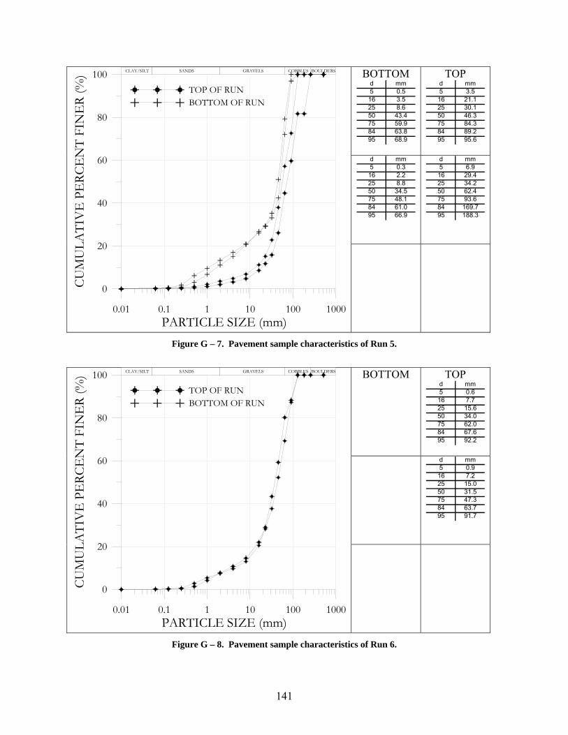
141

BOTTOM d mm5 0.516 3.525 8.650 43.475 59.984 63.895 68.9

TOP d mm5 3.516 21.125 30.150 46.375 84.384 89.295 95.6

d mm5 0.316 2.225 8.850 34.575 48.184 61.095 66.9

d mm5 6.916 29.425 34.250 62.475 93.684 169.795 188.3

0.01 0.1 1 10 100 1000PARTICLE SIZE (mm)

0

20

40

60

80

100CU

MU

LATI

VE

PE

RCE

NT

FIN

ER

(%)

TOP OF RUNBOTTOM OF RUN

CLAY/SILT SANDS GRAVELS COBBLES BOULDERS

Figure G – 7. Pavement sample characteristics of Run 5.

BOTTOM

TOP

d mm5 0.616 7.725 15.650 34.075 62.084 67.695 92.2

d mm5 0.916 7.225 15.050 31.575 47.384 63.795 91.7

0.01 0.1 1 10 100 1000PARTICLE SIZE (mm)

0

20

40

60

80

100

CUM

ULA

TIV

E P

ERC

EN

T FI

NE

R (%

)

TOP OF RUNBOTTOM OF RUN

CLAY/SILT SANDS GRAVELS COBBLES BOULDERS

Figure G – 8. Pavement sample characteristics of Run 6.

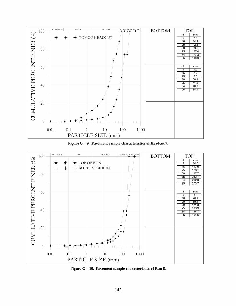
142

BOTTOM

TOP d mm5 7.516 24.425 42.250 83.675 167.084 177.395 190.9

d mm5 0.516 2.225 6.850 20.975 41.884 46.995 64.9

0.01 0.1 1 10 100 1000PARTICLE SIZE (mm)

0

20

40

60

80

100CU

MU

LATI

VE

PE

RCE

NT

FIN

ER

(%)

TOP OF HEADCUT

CLAY/SILT SANDS GRAVELS COBBLES BOULDERS

Figure G – 9. Pavement sample characteristics of Headcut 7.

BOTTOM

TOP

d mm5 24.016 117.925 128.150 187.775 252.784 262.095 273.7

d mm5 8.316 46.125 85.150 171.375 183.984 188.795 194.6

0.01 0.1 1 10 100 1000PARTICLE SIZE (mm)

0

20

40

60

80

100

CUM

ULA

TIV

E P

ERC

EN

T FI

NE

R (%

)

TOP OF RUNBOTTOM OF RUN

CLAY/SILT SANDS GRAVELS COBBLES BOULDERS

Figure G – 10. Pavement sample characteristics of Run 8.

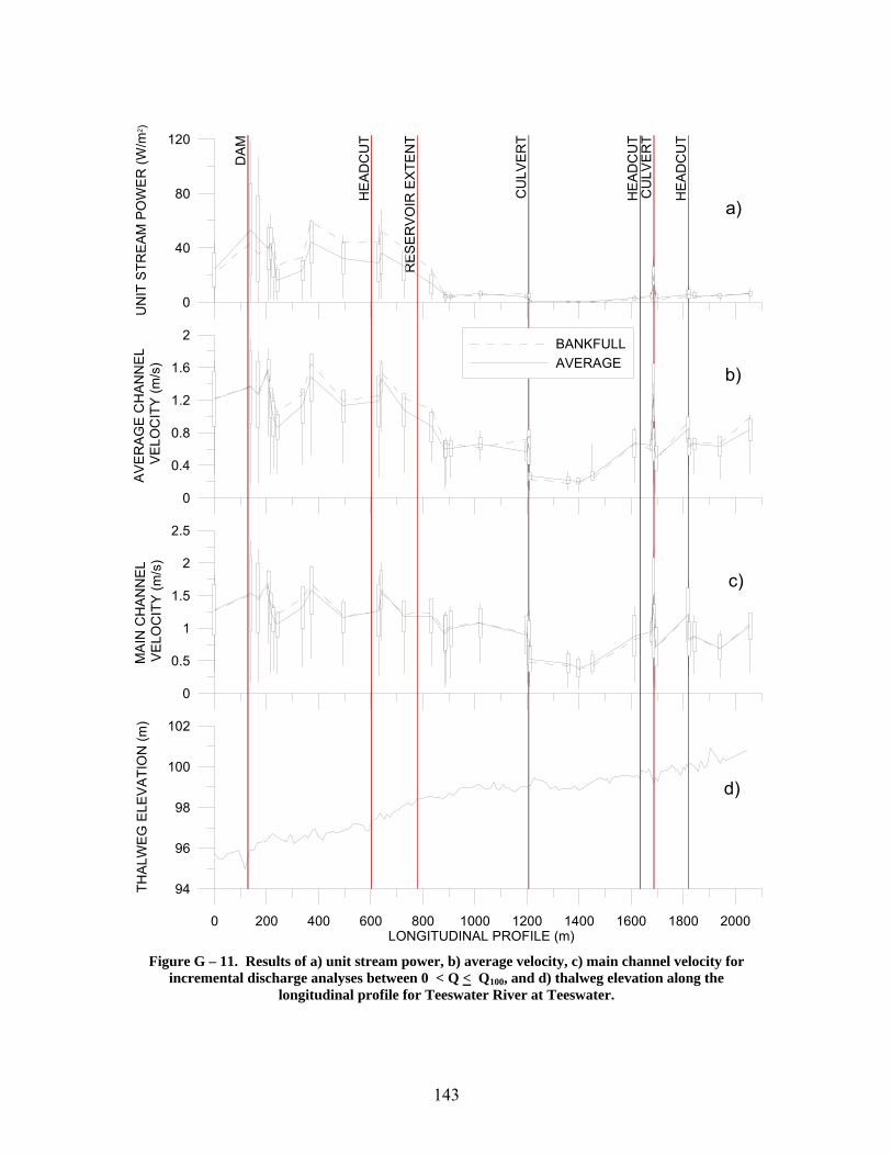
143

0 200 400 600 800 1000 1200 1400 1600 1800 2000LONGITUDINAL PROFILE (m)

94

96

98

100

102

THA

LWE

G E

LEV

ATI

ON

(m)

DA

M

HE

AD

CU

T

RE

SE

RV

OIR

EX

TEN

T

HE

AD

CU

T

HE

AD

CU

T

CU

LVE

RT

CU

LVE

RT

0

0.5

1

1.5

2

2.5

MA

IN C

HA

NN

EL

VE

LOC

ITY

(m/s

)

0

0.4

0.8

1.2

1.6

2

AV

ER

AG

E C

HA

NN

EL

VE

LOC

ITY

(m/s

)

0

40

80

120U

NIT

STR

EA

M P

OW

ER

(W/m

2 )

BANKFULLAVERAGE

b)

a)

c)

d)

Figure G – 11. Results of a) unit stream power, b) average velocity, c) main channel velocity for

incremental discharge analyses between 0 < Q < Q100, and d) thalweg elevation along the longitudinal profile for Teeswater River at Teeswater.

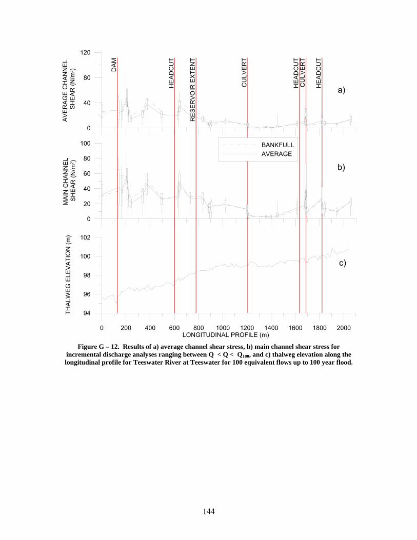
144

0 200 400 600 800 1000 1200 1400 1600 1800 2000LONGITUDINAL PROFILE (m)

94

96

98

100

102

THA

LWEG

ELE

VATI

ON

(m)

DA

M

HE

AD

CU

T

RE

SE

RV

OIR

EX

TEN

T

HE

AD

CU

T

HE

AD

CU

T

CU

LVE

RT

CU

LVE

RT

0

20

40

60

80

100

MA

IN C

HA

NN

EL

SH

EAR

(N/m

2 )

0

40

80

120

AVER

AG

E C

HAN

NE

L S

HE

AR (N

/m2 )

BANKFULLAVERAGE

b)

a)

c)

Figure G – 12. Results of a) average channel shear stress, b) main channel shear stress for

incremental discharge analyses ranging between Q < Q < Q100, and c) thalweg elevation along the longitudinal profile for Teeswater River at Teeswater for 100 equivalent flows up to 100 year flood.

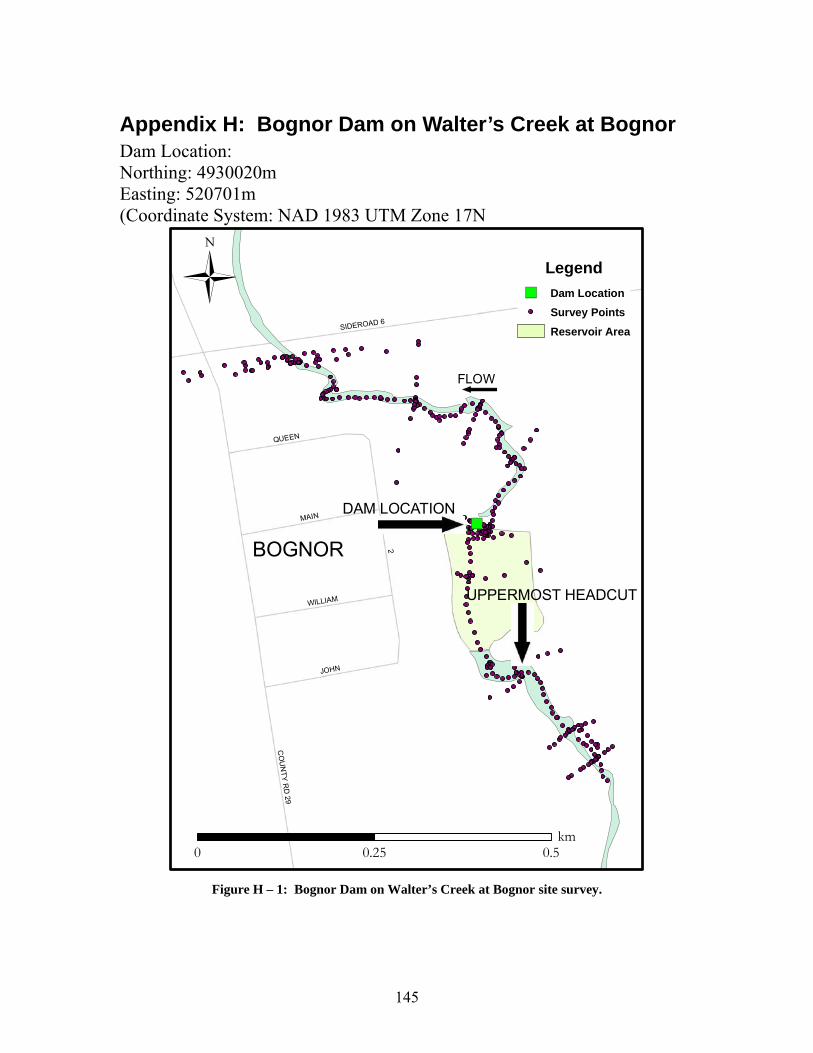
145

Appendix H: Bognor Dam on Walter’s Creek at Bognor Dam Location: Northing: 4930020m Easting: 520701m (Coordinate System: NAD 1983 UTM Zone 17N

")

UPPERMOST HEADCUT

BOGNOR 2

CO

UN

TY RD

29

SIDEROAD 6

MAIN

JOHN

QUEEN

WILLIAM

­ Legend") Dam Location

Survey PointsReservoir Area

0 0.50.25km

FLOW

DAM LOCATION

Figure H – 1: Bognor Dam on Walter’s Creek at Bognor site survey.

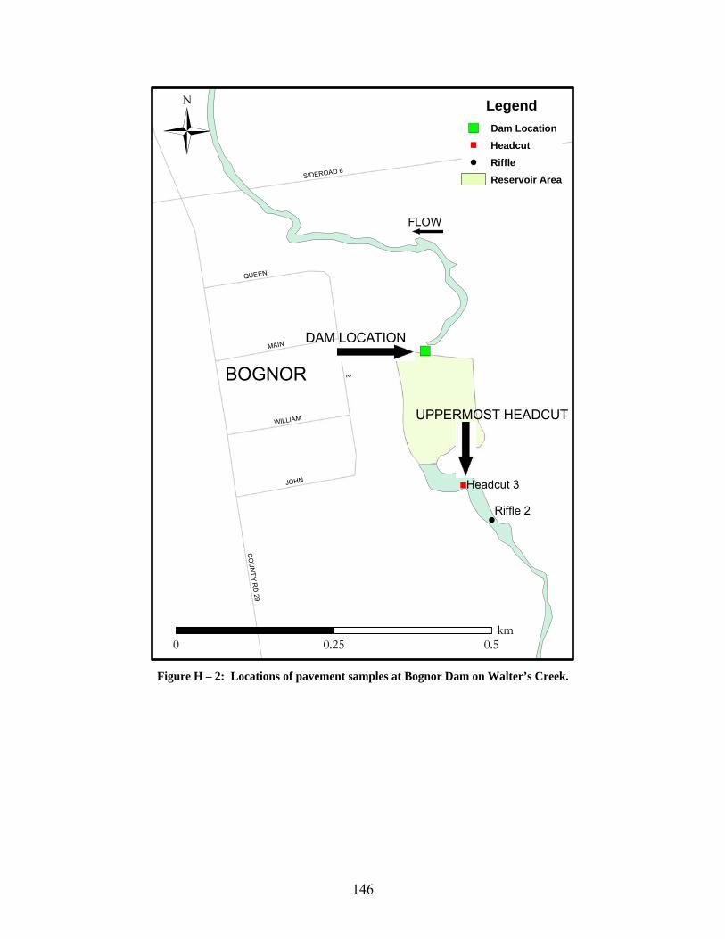
146

")

!

"

UPPERMOST HEADCUT

BOGNOR 2

CO

UN

TY RD

29

SIDEROAD 6

MAIN

JOHN

QUEEN

WILLIAM

Riffle 2

Headcut 3

­Legend

") Dam Location" Headcut! Riffle

Reservoir Area

0 0.50.25km

FLOW

DAM LOCATION

Figure H – 2: Locations of pavement samples at Bognor Dam on Walter’s Creek.

147

BOTTOM

d mm5 2.216 23.325 43.150 69.275 97.984 241.095 266.6

TOP

d mm5 14.716 31.725 43.750 119.475 133.584 139.095 186.4

0.01 0.1 1 10 100 1000PARTICLE SIZE (mm)

0

20

40

60

80

100CU

MU

LATI

VE

PE

RCE

NT

FIN

ER

(%)

TOP OF RIFFLEBOTTOM OF RIFFLE

CLAY/SILT SANDS GRAVELS COBBLES BOULDERS

Figure H – 3. Pavement sample characteristics of Riffle 2.

BOTTOM

TOP

d mm5 0.516 2.025 6.850 31.775 48.884 84.295 124.4

d mm5 8.916 44.025 62.350 89.575 119.184 126.195 135.2

0.01 0.1 1 10 100 1000PARTICLE SIZE (mm)

0

20

40

60

80

100

CUM

ULA

TIV

E P

ERC

EN

T FI

NE

R (%

)

TOP OF RIFFLEBOTTOM OF RIFFLE

CLAY/SILT SANDS GRAVELS COBBLES BOULDERS

Figure H – 4. Pavement sample characteristics of Headcut 3.

148

0 100 200 300 400 500 600 700 800 900 1000 1100LONGITUDINAL PROFILE (m)

242

244

246

248

250

THA

LWEG

ELE

VATI

ON

(m)

DA

M

HE

AD

CU

T

HE

AD

CU

TR

ES

ER

VO

IR E

XTE

NT

SID

ER

OA

D 6

0

0.5

1

1.5

2

2.5

MA

IN C

HA

NN

EL

VEL

OC

ITY

(m/s

)

0

0.5

1

1.5

2

2.5

AV

ER

AG

E C

HAN

NE

LV

ELO

CIT

Y (m

/s)

0

100

200

300U

NIT

STR

EA

M P

OW

ER

(W/m

2 )BANKFULLAVERAGE

b)

a)

c)

d)

Figure H – 5. Results of a) unit stream power, b) average velocity, c) main channel velocity for

incremental discharge analyses between 0 < Q < Q100, and d) thalweg elevation along the longitudinal profile for Walter’s Creek at Bognor.

149

0

50

100

150

200

250

MA

IN C

HA

NN

EL

SH

EA

R (N

/m2 )

0

40

80

120

160

200

AV

ER

AG

E C

HA

NN

EL

SH

EA

R (N

/m2 )

BANKFULLAVERAGE

0 100 200 300 400 500 600 700 800 900 1000 1100LONGITUDINAL PROFILE (m)

242

244

246

248

250

THA

LWE

G E

LEVA

TIO

N

DA

M

HE

AD

CU

T

HE

AD

CU

TR

ES

ER

VO

IR E

XTE

NT

SID

ER

OA

D 6

b)

a)

c)

Figure H – 6. Results of a) average channel shear stress, b) main channel shear stress for

incremental discharge analyses ranging between Q < Q < Q100, and c) thalweg elevation along the longitudinal profile for Walter’s Creek at Bognor.