Embed Size (px)
Citation preview

ARTICLE IN PRESS
0264-8172/$ - se
doi:10.1016/j.m
�CorrespondThe Netherland
E-mail addr
Marine and Petroleum Geology 23 (2006) 931–942
www.elsevier.com/locate/marpetgeo
Upscaling of small-scale heterogeneities to flowunits for reservoir modelling
D. Mikesa,b,�, O.H.M. Barzandjib, J. Bruiningb, C.R. Geelb
aHof van Groenen 21, 1083 JR Amsterdam, The NetherlandsbDelft University of Technology, Department of Applied Earth Sciences, PO Box 5028, NL-2600GA Delft, The Netherlands
Received 14 May 2003; received in revised form 14 April 2005; accepted 13 June 2005
Abstract
The effect of small-scale heterogeneities on fluid flow through a reservoir is determined using one of so called mathematical upscaling
methods, that as such are fairly well established. Less well established, however, are the operations that provide their input, i.e.
construction of reservoir model and acquisition of data. We thereto propose systematic description of facies and bed and systematic data
sampling. We upscale the ensuing model and data through a two-step flow simulation, i.e. first on the flow cell and then on the flow unit
scale. This work provides for a straightforward and easily applicable upscaling method that incorporates the effects of all heterogeneities.
r 2006 Elsevier Ltd. All rights reserved.
Keywords: Upscaling; Flow simulation; Reservoir modelling
1. Introduction
Since it was discovered that small-scale heterogeneitiese.g. cross-bedding have an effect on fluid flow (Kortekaas,1985) studies have addressed their effective bed perme-ability by a number of mathematical methods, viz.averaging, renormalization, homogenisation, and numer-ical flow simulation, in order to determine one- and two-phase permeabilities and capillary pressures. Studies alsoaddressed geometries of facies and beds, i.e. dimensions,distributions, bedding types and the effect of clay layers.
All these methods served to establish the effect of small-scale parameters on a larger scale. This procedure iscommonly referred to as ‘‘upscaling’’. A number ofpublications have addressed so called ‘‘integrated upscalingprocedures’’, generally referring to a procedure of con-structing a reservoir model with upscaling being an integralpart. Considering all publications on this subject we canconclude that all necessary techniques to construct areservoir model have been established. Still, a satisfying
e front matter r 2006 Elsevier Ltd. All rights reserved.
arpetgeo.2005.06.005
ing author. Hof van Groenen 21, 1083 JR Amsterdam,
s. Fax: +31 84 728 50 30.
ess: [email protected] (D. Mikes).
‘‘integrated’’ upscaling procedure has not been designed.Why is this?Let us go through all steps from rock record to reservoir
flow simulation.
(1)
Geometrical model (large and small-scale) comprisinggeological description, facies analysis and facies model.(2)
Data acquisition (sampling, analysis) comprising sam-pling, data analysis and permeability averaging inhomogeneous elements.(3)
Upscaling (small to large-scale) comprising flow cellmodel and calculation of effective flow cell perme-ability.(4)
Reservoir flow simulation comprising petrophysicaldescription, flow units, reservoir flow simulation.Geologists traditionally construct detailed, yet partlyconceptual geological models to characterise a sedimentaryenvironment. Reservoir geologists perform flow simulationon a naively simple reservoir model. Petrophysicistsprovide some theoretical basis for rock properties likeporosity, permeability, wettability. Statisticians and math-ematicians establish methods to calculate production of areservoir.
ARTICLE IN PRESS
Nomenclature
k permeability, L2, m2
kr relative permeabilityS saturation, fractionPc capillary pressure, m/Lt2, Pas interfacial tension, m/t2, N/mg empirical constantl sorting factorj porosity, fraction
Subscripts
o oilw waterwc connate waterwe normalised water (saturation)g gas
D. Mikes et al. / Marine and Petroleum Geology 23 (2006) 931–942932
For the number and quality of geological tools weobserve a decrease from steps 1 to 4. However, for thenumber and quality of mathematical tools we observe adecrease from 4 to 1. But most importantly there seems tobe a trend of conventional geologists focussing on step 1and a bit on step 2 and of reservoir geologists focussing onstep 4 and a bit on step 3. Hence steps 1 and 2 are wellestablished, steps 2 and 3 less.
The fundamental question of upscaling is how toincorporate small-scale structures in a large-scale reservoirmodel, without a full-scale model at the resolution of alamina? The answer is of course to incorporate effects ofsmall-scale structures instead. Since geological structuresare strictly hierarchical of nature, the upscaling procedureshould conform to this hierarchy.
A number of review papers give a concise overview ofupscaling procedures (Ewing, 2000; Pickup and Stephen,2000; Christie, 2001; Moulton et al., 1998). Traditionalmethods use averaging, renormalisation or homogenisa-tion, while more modern methods use Dykstra–Parsonscoefficient, pseudo functions, flow simulation, streamline,finite difference, effective medium or efficient flux. Thesemethods are good as such. They appreciate the naturalhierarchy of geological structures, repetitiveness of struc-tures and the mathematical algorithms are robust. Thenwhat are the problems?
The problems are one or more of the following. Themethods on certain elements of the geology and/ormathematics, even the ones that carry the name ofintegrated procedures. They do not incorporate featuresof geological elements explicitly viz. facies distribution,facies boundaries and bedding characteristics. They do notperform sampling and sample analysis systematically. Theydo not calculate relative permeability and capillarypressure of individual laminae. Hence, the reservoir modelrepresents the reservoir inadequately and upscaling isperformed on inaccurate data. And even so, most methodsare too complex to be used routinely.
The objective of this study is neither to invent newmathematical algorithms nor new geological techniques,but to present a procedure that focuses on the geologicalmodel. This paper presents the upscaling part of theprocedure and a test on an example to demonstrate itsapplication and efficiency. The other elements of the
procedure are presented in three papers, i.e. facies (Mikesand Geel, 2006), bed (Mikes and Bruining, 2006), sampling(Mikes, 2006). They give the scientific ground for thisapproach.The idea is to focus attention on geological features and
their characteristics to hydraulic flow. On the one handgeometries like shape, dimension, flow boundary, spatialdistribution, repetition and the like. On the other handheterogeneities like one- and two-phase permeability,contrasts, trends, relative permeability, capillary pressureand the like.We focus on laminae, because we consider a bed the
smallest heterogeneous element and a lamina the largesthomogeneous element and therefore intentionally disre-gard intra-lamina trends. We do not consider the funda-mentals of petrophysical properties like wettability,interfacial tension, adhesion, pore shape etc. The samegoes for relative permeability and capillary pressure. Webelieve that the first priority is to construct an adequatereservoir model and assign it appropriate hydraulic flowproperties. In short, we want to supply adequate data tothe upscaling algorithm.To demonstrate the value of this method, we apply it to
the model described in the SPE ninth comparative study(Killough, 1995). The results show that small-scale hetero-geneities must be explicitly taken into account. Ourprocedure provides a straightforward method to accom-plish this routinely in reservoir modelling. The mainpurpose of this work is twofold: (1) improve thetransformation of geological model to reservoir model byan ‘‘a-priori’’ deterministic description; (2) provide asimple and straightforward procedure to upscale reservoirheterogeneity.To this end we propose a four-step procedure (Fig. 1):
(1) Model construction: identification of flow cells and flowunits. (2) Parameter assignment: sampling of laminapermeability and calculation of capillary pressure andrelative permeability of laminae. (3) Micro-simulation:static (or steady state) flow simulation on flow cells. (4)Macro-simulation: assignment of the ensuing effectivephase permeabilities and capillary pressures to the flowunits and dynamic flow simulation on the reservoir.We started this study with the intention to sample
permeability on outcrops of so-called ‘reservoir analogues’.

ARTICLE IN PRESS
Fig. 1. Schematic representation of the four-step upscaling procedure of
this work. Step 1: Model construction, consisting of geological and
reservoir model and assignment of its elements. Step 2: Parameter
assignment, consisting of permeability sampling, data analysis, and
calculation of relative permeability and capillary pressure. Step 3: Micro
simulation, consisting of numerical flow simulation on all flow cell models
of the reservoir, yielding effective one- and two-phase permeabilities, and
capillary pressures. Step 4: Macro simulation consisting of numerical flow
simulation on the entire reservoir, yielding production history. Steps 1 and
2 form reservoir characterisation. Steps 3 and 4 form numerical flow
simulation.
Table 1
Six-scale hierarchy of heterogeneity levels for facies and reservoir models
in this study
Reservoir units Geological units Facies example
Sequence
Parasequence set Alluvial plain
Facies association/parasequence River
Flow-unit Facies Meander belt
Flow-cell Bed Trough bed
Lamina Foreset
Geological key elements are facies and bed. Reservoir key elements are
flow unit and flow cell.
D. Mikes et al. / Marine and Petroleum Geology 23 (2006) 931–942 933
Following its more or less predefined course we encoun-tered many difficulties. Existing probe-permeametersproved inaccurate. Existing sampling strategies and dataanalysis proved inappropriate. The outcrops proved to bealtered. Existing geological descriptions proved inade-quate. Existing upscaling procedures proved too complex.
Facing so many uncertainties we decided to construct apressure-depletion probe-permeameter and to sample only
on fresh cores from producing hydrocarbon reservoirs. Weconstructed the instrument, calibrated it extensively onnatural and artificial homogeneous and heterogeneous coreplugs and it proved close to perfect (Waal van de et al.,1998). Then we confronted a problem of political nature.No oil-company was willing to borrow us a fresh reservoircore. We ended up with a 10 years old core, altered just likean outcrop.Although we performed measurements on all our out-
crop samples and core, we realised that none of these wasrepresentative of a true reservoir. Frustrated by our lack ofdata, we changed strategy. We decided to construct anupscaling procedure that would be straightforward, effi-cient and routinely applicable. The basis of it would be theexplicit incorporation of hydraulic features of geologicalelements.
2. Methods
We propose a four-step procedure (Fig. 1): (1) Systema-tic description of facies and beds; Assignment of flow unitsand flow cells and construction of geological model andreservoir model. (2) Systematic data sampling and analysis;Sampling and analysis of lamina permeability. Calculationof capillary pressure and relative permeability of laminae.(3) Systematic ‘upscaling’ of lamina permeabilities; Nu-merical flow modelling on flow cells. Input is one- and two-phase permeability and capillary pressure curve of lamina.Output is the effective flow cell values of these. (4)Reservoir flow modelling; Numerical modelling on reser-voir. Input is the effective flow cell one- and two-phasepermeability and capillary pressure of flow unit. Output isthe effective reservoir values of these and the productioncurve. Parts 1 and 2 are entirely original. Parts 3 and 4might not be new as such, but they make the procedurecomplete.We construct the geometric model by way of a six-scale
hierarchy, viz. lamina - bed - facies - facies associa-tion/parasequence - systems tract/parasequence set -sequence (Table 1), which need not all be used for everyreservoir. We consider the (sedimentary) facies a body ofrock with similar sedimentary properties (read: repetitionof one bed), the flow unit a body of rock with similar

ARTICLE IN PRESS
Fig. 2. Geological model of the fluvial system used in this study, the first
part of step 1 (Fig. 1).
D. Mikes et al. / Marine and Petroleum Geology 23 (2006) 931–942934
hydraulic properties (read: repetition of one flow cell), thebed a body of rock with similar sedimentary properties(read: repetition of two laminae), and the flow cell a bodyof rock with similar hydraulic properties (read: repetitionof two laminae).
We define a representative elementary volume (REV) foreach heterogeneity, which may be a periodic unit cell(PUC) if repetitive. According to van Lingen (1998) thelamina is the REV/PUC for the crossbed, the crossbed isthe REV/PUC for the Flow Unit and the flow unit is theREV of the reservoir model. Crossbed and facies are thuskey elements.
Essentially the crossbed corresponds to the flow cell andthe facies to the flow unit (Table 1), but there are somedifferences. Facies have an irregular shape (Fig. 1), whereasflow units are geometrically simplified versions of facies. Inthe reservoir model one flow unit is build up of numerousidentical grid blocks (Fig. 1). A crossbed and foreset-laminae have an irregular shape and change along a facies,whereas a flow cell in our case has a rectangular shape andaverage properties of crossbeds in the flow unit andlaminae are planes.
If a facies consists of a number of zones with differentbedding types, it is to be split up into the same number ofsub-facies. If variation is systematic, the flow cell itself canbe divided into zones with different characteristics. Forexample, a consistent vertical sequence throughout thefacies or vertical grading within the crossbeds or claydrapes as bottomsets, as is the case in a pointbar.
We assume, that for one bedding type (within a facies),crossbed dimensions are normally distributed, laminathickness to be trimodal and lognormally distributed, andlamina permeability to be trimodal and lognormallydistributed. We hence average intra-lamina thickness andintra-lamina permeability via simple arithmetic averaging.
We use simulation on a smaller scale to obtain effectiverelative permeability and capillary pressure functions of theflow cell (Christie, 1996; Christie and Clifford, 1997). Setup in the x, y, z direction with no flow boundary conditionsalong the sides, p ¼ 1 at the inlet, p ¼ 0 at the outlet. Wesolve the equations and sum the fluxes. Then we calculatethe effective directional relative permeabilities and capil-lary pressures. This upscaling method has the advantage tobe easy to implement in reservoir flow simulation routine.
We chose for bi-dimensional flow cell simulation, but inthe future we might use tri-dimensional simulation instead.Nonetheless, any of the existing procedures might do, e.g.averaging, renormalization, homogenisation, pseudoisa-tion, streamline method, effective flux calculation.
As an example we construct a hypothetical reservoirconsisting of a meandering river sequence. In this case wemake the model naively simple to consist of three faciesonly, viz. channel, pointbar, and floodplain, each havingone repetitive element. This is one bedding type forfloodplain (horizontal bedding) and channel (trough cross-bedding) and one specific succession of bedding typesfor the point-bar (large trough bedding at the base,
small trough bedding in the middle and ripple bedding atthe top).We implement our model in the model of the SPE ninth
comparative study (Killough, 1995) to demonstrate theapplicability of our method and to compare results. Thereare three important points we like to emphasise. (1) Theway of incorporating small-scale heterogeneities in areservoir model is significant for reservoir performanceestimation. (2) The upscaling procedure for averagedrelative permeability and capillary pressure deals withcapillary trapping in foreset laminae. (3) The procedure iseasy to implement in the current infrastructure ofpetroleum companies and institutes.
2.1. Geological model
To demonstrate the procedure we examine a highlyheterogeneous reservoir deposited in a fluvial environment.Fluvial reservoirs are known to be heterogeneous on a widerange of scales (Weber, 1986). For our purpose we generatea model in four steps using five different scales (Table 1).The largest scale comprises the entire reservoir (para-
sequence set) and consists of several parasequences(Fig. 2A). The parasequences consist of three facies viz.floodplain, pointbar, and channel-fill (Fig. 2B). A typicalpointbar consists of a series of concentric layers, whichdip down toward the outer bend of the river. Sometimesthese layers are separated by thin shale streaks thatextend from the top to halfway the bottom. The channelfill may contain sand in which case there is abundanttrough crossbedding, or it may contain shale in a classic

ARTICLE IN PRESS
Table 2
List of input parameters for the flow-cell models
Parameter Channel Point bar Flood plain
U M L
D. Mikes et al. / Marine and Petroleum Geology 23 (2006) 931–942 935
oxbow-lake configuration. In this case, we have chosen tomodel a mainly sandy channel-fill.
Each facies consists of one bedding type (Fig. 2C):horizontal bedding in the floodplain, lateral accretion inthe pointbar, and trough crossbedding in the (sandy)channel fill. Each bed type consists of bottomset laminaeand two types of foreset laminae, horizontal bottomsetlaminae are fine grained, inclined foreset laminae aremedium or coarse grained. Lateral accretion bedding is innature internally composed of trough crossbedding alignedin the direction of paleoflow. This superimposed cross-bedding complicates matters severely and has therefore inthe present study been omitted.
2.2. Reservoir model
The reservoir model is a direct transformation of thegeological model. Thus, the large-scale model consists oflayers (Fig. 3A) for which in this case thickness and flowunit size are given by Killough (1995). Within these layersthe floodplain, pointbar, and channel fill flow units areplaced (Fig. 3B). Identical flow units compose one facies.Each flow unit consists of several identical flow-cells,the equivalent of the bedding type in the geological model(Fig. 3C). We make an important simplification here:flow cells have the same orientation within each flowunit. Thus, lateral accretion surfaces in the pointbars andtrough crossbedding in the channel fill always dip in the
Fig. 3. Reservoir model of the fluvial system used in this study, the second
part of step 1 (Fig. 1). Note that flow unit and flow cell of lateral accretion
are identical. The reason for this is, that the PUC covers the entire height
of the point bar, consisting of three different bedding types (Fig. 6).
X-direction. As a result, each of the flow units has the sameproperties throughout the model.Dimensions for the flow cells were inferred from the
geological model and are listed in Table 2. At a smallerscale, each flow cell is made up of alternating laminae, towhich different permeabilities are attributed. Typicallamina permeability values were compiled from literatureand from our own data (Table 3). These values weresimplified to the extent that we only have three perme-abilities: 10, 50, and 200mD. The floodplain has horizontalbedding with an alternation of 10 and 50mD. The channelfill has crossbedding (alternation of 50 and 200mDlaminae) or it is shale filled (10mD). The pointbar hasthree superimposed regions of equal thickness: the lowerpart consists of cross bedding only (alternation of 50 and200mD); the middle part contains cross bedding withoccasional clay drapes (alternation of 50 and 200mD andthe clay drapes 10mD). The upper part is horizontalbedding with an alternation of 10 and 50mD. In this caseflow cell and grid block have equal thickness.
Table 3
List of permeabilities for the flow-cell models
Parameter Channel Point bar Floodplain
U M L
KC (mD) 200 — 200 200 —
KF (mD) 50 50 50 50 50
KB (mD) 10 10 10 — 10
Keff (mD) 87.0 34.7 29.6
Keff,model (mD) 37.0
Keff,spe (mD) 94.0
jriver (—) 0.3
jave,spe (—) 0.13
The permeability values for the flow cells are educated guesses based on
literature. Keff is effective permeability; river indicates the model presented
here; spe refers to the ninth SPE model (Killough, 1995); j denotes
porosity; ave is average; C, F, B indicate coarse-, fine grained foreset and
bottomset.
T (cm) 12.55 10 10 10 24
W (cm) 1 1 1 1 1
L (cm) 50 50 50 50 50
a (1) 10–30 0 30 30 0
C gr.block # (—) 925 — 264 225 —
F gr.block # (—) 925 250 264 225 600
B gr.block # (—) 200 250 22 — 600
Total gridblock # (—) 2050 1600 1200
T, W, L stand for thickness, width, length of the model; C, F, B indicate
coarse-, fine grained foreset and bottomset; a denotes foreset dip; # means
number.

ARTICLE IN PRESSD. Mikes et al. / Marine and Petroleum Geology 23 (2006) 931–942936
The model is a prototype of a meandering river systemand its geometry is mostly obtained from Galloway andHobday (1983) and the values are guesses based on anoverview of published examples. The permeability value forthe bottomset might be high, but others even use valuesequal to foreset permeability. The channel is in natureoften conserved as separated clay plugs. This would notyield a continuous channel as in Fig. 2, but horseshoeelements of clay filled channel bends, with free passagesbetween them as in Fig. 4.
2.3. Micro-simulation
Here we describe the procedure of obtaining upscaledphase permeability curves and capillary pressures for thethree bed types constituting the reservoir. These upscaledpermeabilities are derived in a three-step process, i.e. twoupscaling steps and the actual simulation.
First we assign Brooks–Corey relative permeabilityfunctions to the high and low permeable foresets and tothe bottom sets constituting the beds (Lingen van, 1998).
kw ¼ kk0rw
Sw � Swc
1� Swc
� �ð2=lÞþ3:¼ kk0rwSð2=lÞþ3wc , (1)
ko ¼ kk0roð1� SwcÞ2 1� Sð2=lÞþ1wc
� �, (2)
Fig. 4. Three-dimensional geometries of sand bodies of braided, mean-
dering, and stable/anastomosed rivers (adapted from Galloway and
Hobday, 1983). The rest of the facies being clay they are impermeable and
do not significantly contribute to the flow of fluids.
Fig. 5. Capillary-pressure- and relative-permeability curves for the three lamina
to water, Krow is relative permeability to oil in presence of water, Pcow is capil
Pc ¼ gsow
ffiffiffiffijk
r12� Swc
Sw � Swc
� �1=l
. (3)
For convenience we use the same values as Lingen van(1998); empirical constant g ¼ 0.79, connate water satura-tion Swc ¼ 0.0, sorting factor l ¼ 1.5, porosity j ¼ 0.3 andinterfacial tension between oil and water sow ¼ 0.03N/m.End point permeabilities for water and oil are takenk0rw ¼ 1 and k0ro ¼ 1. Permeabilities are summarized inTable 3 and would normally have been obtained fromprobe-permeameter measurements on cores. We wouldhave used image analysis to estimate the sorting factor, buthere we used an average value l ¼ 1.5 for both foresets andbottom sets. In this way we completely assigned the relativepermeability and capillary pressure fields for each of thethree lamina types in our bedding models (Fig. 5). Theaspect that trapping is controlled by wetting state is outsidethe scope of this article (Huang et al., 1996) and we confineinterest to water wet media.In the second step, the notions REV and PUC play an
essential role. Following Bear (1972) we define the REV fora property as the averaging volume beyond which theaverage value of a property remains more or less un-changed. The PUC is a building block of the REV that canbe considered periodic for all practical purposes. Here weequate the PUC to the flow cell. Because of periodicityaverage properties of the PUC are representative for theREV.Thus there is one flow cell for every facies, i.e.
crossbedding for the channel, lateral accretion for thepointbar and horizontal bedding for the floodplain (Figs. 2and 3). We perform 2D simulations on each flow cell(Fig. 6). For a relatively small section we may assume thatduring reservoir production it will go through a slowlyvarying set of quasi steady states. This assumption is alsoimplicit in other upscaling methods e.g. homogenisation.In accordance with previous authors, we inject and
produce through two opposite faces of a rectangular blockand use no-flow conditions through the other four faces.This approach ignores permeability anisotropy. We use thisapproach as a first example, although modern simulatorscan indeed handle non-diagonalised tensor permeabilityand crossbedded structures are known to require full-tensor permeability (Pickup et al., 1995). The initial oil and
types used in this study for all three flow-cells. Krw is relative permeability
lary pressure between oil and water.

ARTICLE IN PRESSD. Mikes et al. / Marine and Petroleum Geology 23 (2006) 931–942 937
water saturation in the flow cell are determined byassuming a given capillary pressure, Pc ¼ 107 kPa. Wecontinue flooding until steady state is reached.
The third step is the computation of relative permeabilityand capillary pressure from the simulation results. We use
Fig. 6. The flow-cell models for channel, point bar, and floodplain for
STARS. On these three models the two-dimensional small-scale flow
simulations have been performed. Flow is from left to right. The three flow
cells are built with three lamina types: coarse foreset (200mD), fine foreset
(50mD), and bottomset (10mD). Inlets show individual grid cells. Shades
denote permeabilities: White (200mD), light grey (50mD), and dark grey
(10mD).
Fig. 7. Capillary-pressure- and relative-permeability curves for horizontal fl
capillary pressures have been chosen to be identical to the water–oil relati
permeability to oil in presence of water, Pcow is capillary pressure between oil
Darcy’s law in which we substitute the flow of oil and watertogether with the average phase pressure differencebetween the injection and production side to derive thephase permeabilities with Darcy’s law. Also, the average oilminus the average water pressure is the capillary pressure.Finally we calculate the average saturation in the flow cell.In this way, we obtain one point in the phase permeability-saturation curve and capillary pressure-saturation curve.We continue to use the same procedure with water/oil
injection mixtures ranging from zero to 100% oil, withsteps of 10%. In this way the upscaled phase permeabilitiesand capillary pressures for the channel beds, the point barbeds and the flood plain beds are obtained. We repeat thesame procedure only allowing for flow in the verticaldirection.In the simulation considered we have three-phase oil–
water–gas flow. Hence three-phase permeabilities arerequired. Here we use STONE II. A somewhat betterapproach would be to perform three-phase (steady state)simulations, instead of the two-phase simulations describedabove. The results would, however, be history dependentand hence three-phase upscaling is considered outside thescope of this article. If, however, we do such a study in theappraisal stage, when no free gas is liberated, a black oilsimulator might be appropriate.These results are not suitable yet for implementation into
a standard simulation run, because the relative perme-ability and capillary pressure are anisotropic. Hence wemake one further simplification. We calculate the averageratio between relative permeabilities in the vertical andhorizontal directions. We also calculate the one-phasepermeability anisotropy from one-phase simulations. Theproduct of the average ratio with the one-phase anisotropyfactor determines the effective permeability anisotropy. Weuse the relative permeability and capillary pressureobtained from the horizontal flow simulation.
2.4. Results for upscaled permeabilities
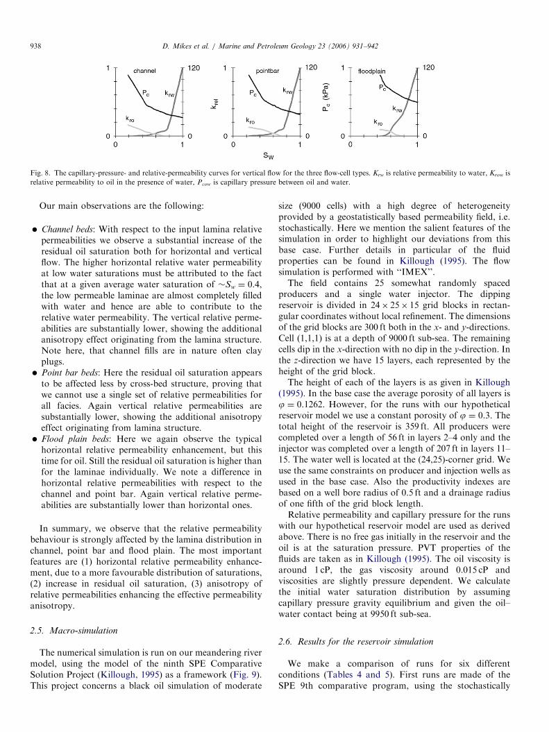
The results from the micro-simulation are summarised inFig. 7 for horizontal flow and in Fig. 8 for vertical flow.The relative permeability for oil/gas is chosen identical tothe relative permeability for water/oil (Berry et al., 1992).
ow for the three flow-cell types. The oil-gas relative permeabilities and
ve permeabilities. Krw is relative permeability to water, Krow is relative
and water.
ARTICLE IN PRESS
Fig. 8. The capillary-pressure- and relative-permeability curves for vertical flow for the three flow-cell types. Krw is relative permeability to water, Krow is
relative permeability to oil in the presence of water, Pcow is capillary pressure between oil and water.
D. Mikes et al. / Marine and Petroleum Geology 23 (2006) 931–942938
Our main observations are the following:
�
Channel beds: With respect to the input lamina relativepermeabilities we observe a substantial increase of theresidual oil saturation both for horizontal and verticalflow. The higher horizontal relative water permeabilityat low water saturations must be attributed to the factthat at a given average water saturation of �Sw ¼ 0.4,the low permeable laminae are almost completely filledwith water and hence are able to contribute to therelative water permeability. The vertical relative perme-abilities are substantially lower, showing the additionalanisotropy effect originating from the lamina structure.Note here, that channel fills are in nature often clayplugs. � Point bar beds: Here the residual oil saturation appearsto be affected less by cross-bed structure, proving thatwe cannot use a single set of relative permeabilities forall facies. Again vertical relative permeabilities aresubstantially lower, showing the additional anisotropyeffect originating from lamina structure.
� Flood plain beds: Here we again observe the typicalhorizontal relative permeability enhancement, but thistime for oil. Still the residual oil saturation is higher thanfor the laminae individually. We note a difference inhorizontal relative permeabilities with respect to thechannel and point bar. Again vertical relative perme-abilities are substantially lower than horizontal ones.
In summary, we observe that the relative permeabilitybehaviour is strongly affected by the lamina distribution inchannel, point bar and flood plain. The most importantfeatures are (1) horizontal relative permeability enhance-ment, due to a more favourable distribution of saturations,(2) increase in residual oil saturation, (3) anisotropy ofrelative permeabilities enhancing the effective permeabilityanisotropy.
2.5. Macro-simulation
The numerical simulation is run on our meandering rivermodel, using the model of the ninth SPE ComparativeSolution Project (Killough, 1995) as a framework (Fig. 9).This project concerns a black oil simulation of moderate
size (9000 cells) with a high degree of heterogeneityprovided by a geostatistically based permeability field, i.e.stochastically. Here we mention the salient features of thesimulation in order to highlight our deviations from thisbase case. Further details in particular of the fluidproperties can be found in Killough (1995). The flowsimulation is performed with ‘‘IMEX’’.The field contains 25 somewhat randomly spaced
producers and a single water injector. The dippingreservoir is divided in 24� 25� 15 grid blocks in rectan-gular coordinates without local refinement. The dimensionsof the grid blocks are 300 ft both in the x- and y-directions.Cell (1,1,1) is at a depth of 9000 ft sub-sea. The remainingcells dip in the x-direction with no dip in the y-direction. Inthe z-direction we have 15 layers, each represented by theheight of the grid block.The height of each of the layers is as given in Killough
(1995). In the base case the average porosity of all layers isj ¼ 0.1262. However, for the runs with our hypotheticalreservoir model we use a constant porosity of j ¼ 0.3. Thetotal height of the reservoir is 359 ft. All producers werecompleted over a length of 56 ft in layers 2–4 only and theinjector was completed over a length of 207 ft in layers 11–15. The water well is located at the (24,25)-corner grid. Weuse the same constraints on producer and injection wells asused in the base case. Also the productivity indexes arebased on a well bore radius of 0.5 ft and a drainage radiusof one fifth of the grid block length.Relative permeability and capillary pressure for the runs
with our hypothetical reservoir model are used as derivedabove. There is no free gas initially in the reservoir and theoil is at the saturation pressure. PVT properties of thefluids are taken as in Killough (1995). The oil viscosity isaround 1 cP, the gas viscosity around 0.015 cP andviscosities are slightly pressure dependent. We calculatethe initial water saturation distribution by assumingcapillary pressure gravity equilibrium and given the oil–water contact being at 9950 ft sub-sea.
2.6. Results for the reservoir simulation
We make a comparison of runs for six differentconditions (Tables 4 and 5). First runs are made of theSPE 9th comparative program, using the stochastically

ARTICLE IN PRESS
Table 4
List of properties for the flow-unit model
Channel belt along
strike
Channel belt along
dip
SPE stochastic K-
field
N1 N1v N3 N3v HSPE VSPE
Pc Pc,ow,calc Pc,,ow,calc Pc,ow,spe
Kr,ow Kr,og upsc Kr,ow upsc Kr,ow,spe
Kr,og Kr,ow upsc Kr,og upsc Kr,og,spe
K Kmodel Kmodel Kspe
Kh/Kv (eff) 100 5.6 100 5.6 100 5.6
Tlayer Variable Variable Variable
Gridblock # Pointbar: 160 Pointbar: 152 600
Floodplain: 375 Floodplain: 384
Pcow is capillary pressure between oil and water, Krow is relative
permeability to oil in presence of water, Krog is relative permeability to
gas in presence of oil, K is permeability, Kh is effective horizontal
permeability, Kv is effective vertical permeability, Tlayer is the gridblock
thickness, # stands for number, river refers to our model, spe refers to the
model in the SPE ninth comparative study (Killough, 1995); calc means
analytically calculated; N1 is our river model with the channel belt along
strike of the model. N3 is the same model with the channel belt along dip
(Fig. 9). SPE, N1, N3 have Kh/Kv ¼ 100, SPEv, N1v, N3v have Kh/
Kv ¼ 5.6.
Fig. 9. Along strike (scenarios N1, N3) and along dip (scenarios N1v,
N3v) flow simulation models for IMEX. Blocks denote individual grid
cells. Flow in the model is up dip. The model is inclined as in the ninth
SPE comparative study (Killough, 1995), and grid blocks themselves are
horizontal. Number, height, and average permeability of grid blocks
correspond to Killough (1995). Shades indicate the three grid cells (flow
units) used, i.e. white (channel), light grey (pointbar), and dark grey
(floodplain).
D. Mikes et al. / Marine and Petroleum Geology 23 (2006) 931–942 939
generated reservoir model and all the input data ofKillough (1995), whose relative permeabilities and capillarypressures are shown in Fig. 10. However, we like tocompare the situation with two effective permeabilityanisotropy ratios. First we use a ratio of horizontal tovertical permeability of 100 (indicated as SPE). Then weuse an effective permeability ratio of 5.6 (SPEv). The otherfour cases concern our hypothetical reservoir modeldeveloped in this paper. We use the channel belt along
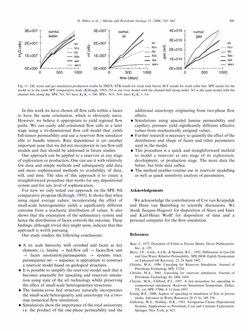
strike with effective permeability anisotropy ratios of 100(N1), and 5.6 (N1v). The last two runs concern a modelwith the channel belt along dip, with again anisotropyratios of 100 (N3) and 5.6 (N3v).Fig. 11 presents the most conspicuous results of the six
runs. Shown are the cumulative oil, gas and waterproductions. Admittedly the results of our reservoir model(N1, N1v, N3, N3v) with porosities j ¼ 0.3 are difficult tocompare with SPE and SPEv with average porosities ofj ¼ 0.13 (see Table 5), but it is important to note thedifferences between our different model runs. We alsoobserve that the different anisotropy factors have a largeeffect on the cumulative productions from the stochasti-cally generated reservoirs.For the hypothetical river model, there appears to be a
slightly more favourable (lower) water production and lessfavourable oil recovery (lower) from reservoirs where theanisotropy factor is highest. This is to be expected as theinjection well is injecting water in the bottom part of thereservoir, and oil is produced near the top. Whether thechannel belt is along strike or along dip has little effect.This can possibly be attributed to a more or less symmetricsituation with respect to the injection well and apparently aslight effect of dip in this particular situation.For the conditions shown the gas oil ratio for our
hypothetical reservoir model is still approximately equal tothe solution gas oil ratio indicating that we are still beforefree gas breakthrough. Our most important result is,however, that we have shown that facies based reservoirmodels can be simplified in a way that makes these modelsamenable to upscaling and reservoir simulation withoutlosing the effects of the small scale. Our results present thebasic concept of a procedure that can be applied usingmore sophisticated aspects in the future.

ARTICLE IN PRESS
Table 5
Initial values and production results for the different simulation scenarios
SPE SPEv N1 N1v N3 N3v
Total pore volume (106 STB) 453 1324 1324
Initial oil in place (106 STB) 186 234 261
Mobile oil volume (106 STB) 156 82 92
Total solution gas volume (109 SCF) 259 325 327
Free gas volume (109 SCF) 0 0 0
Water volume (106 STB) 246 1061 1063
Cumulative oil produced (106 STB) 17.5 25.2 25.9 27.1 25.5 27.2
Cumulative gas produced (109 SCF) 71.1 101 29.2 31.2 28.4 30.9
Cumulative water produced (106 STB) 2.1 1.6 18.2 23.7 18.9 24.6
Cumulative water injected (106 STB) 1.5 2.5 2.6 3.9 2.7 4.0
STB stands for stock tank barrel, SCF stands for stock cubic feet. SPE stands for the model as in the ninth SPE comparative study (Killough, 1995). N1 is
our river model with the channel belt along strike. N3 is the same model with the channel belt along dip (Fig. 9). SPE, N1, N3 have Kv/Kh ¼ 100, SPEv,
N1v, N3v have Kv/Kh ¼ 5.6.
Fig. 10. Capillary-pressure- and relative-permeability curves for the SPE
model (Killough, 1995). Krw is relative permeability to water, Krow is
relative permeability to oil in the presence of water, Pcow is capillary
pressure between oil and water. Krg is relative permeability to gas, Krog is
relative permeability to oil in presence of gas, Pcog is capillary pressure
between oil and gas.
D. Mikes et al. / Marine and Petroleum Geology 23 (2006) 931–942940
3. Discussion/conclusions
To justify our simplifications with regard to permeabilityand geometry of crossbeds, we argue that these simplifica-tions do not yield the largest error in the upscalingprocedure. We state, that the largest errors occur in thefacies interpretation (uncored facies, misinterpretation),bottomset characteristics (bottomset permeability andcontinuity), relative permeability curves (residual oilsaturation and connate water saturation), capillary pres-sure curves (entry pressure, displacement pressure), andinvestigated area (covering �1� 10�8 of the reservoirvolume).
This is why we deliberately choose to incorporate allaspects in one procedure, instead of detailing on fewelements of the procedure, disregarding others. Thestrength of the procedure is the calculation of relativepermeabilities and capillary pressures for the laminae andin the physical incorporation of laminae into the upscalingprocedure. The other strong point is its simplicity thatallows us to study the effect of variations in parametervalues.
Our upscaling procedure is an attempt for a bettersynthesis of all aspects in upscaling. Ideally, we would have
tested it on a reservoir that has been producing for a longnumber of years. However, we were not so fortunate to gainaccess to production data or to fresh cores from ahydrocarbon reservoir. Those who have access can easilydo testing themselves. Those that critic simplification at anypoint of the procedure, can simply add sophistication at will.Where the statistical validity of quantitative data is
missed, we refer to the many data that have been publishedviz.: (1) sampling of lamina permeabilities with instrumentsthat were visibly not well calibrated and (2) distributions oflamina permeabilities that were visibly incorrectly sampled.We prefer a correct theory with few samples instead of noor an incorrect theory based on many incorrect samples.Quantitative geometrical data are best acquired from the
reservoir from wells, cores, and seismic lines. If notavailable an estimate of minimum and maximum valuesof parameters is to be made. In the modelling we then takeminimum and maximum values for all parameters and seetheir effect on the result.Nonetheless, statistically significant quantitative geome-
trical data are difficult to acquire. Seismic lines mightresolve parasequences, but not facies. Stratigraphic sec-tions supply (cross) bed thickness, but not width and lengthof individual (cross) beds, although suggested by manyauthors. Well logs and cores supply bed thickness, but notmaximum thickness for a continuous set of trough cross-beds. Well logs and cores supply lamina thickness and dips.Cores also supply lamina permeabilities, but yield verypoor lateral coverage.We propose parasequence boundaries to be barriers and
facies boundaries to be conductors to flow. We argue that aparasequence boundary inherently represents some time ofnon-deposition and/or reworking enough to consolidatethe surface and render it significantly less permeable thanthe underlying facies. We argue that a facies boundarywithin a parasequence is a gradual transition from onelithology to another that doesn’t limit flow. Theseassumptions would require testing for every case, but it’sdifficult to obtain permeability values from such aboundary.
ARTICLE IN PRESS
Fig. 11. Oil, water and gas simulation production results by IMEX. STB stands for stock tank barrel, SCF stands for stock cubic feet. SPE stands for the
model as in the ninth SPE comparative study (Killough, 1995). N1 is our river model with the channel belt along strike. N3 is the same model with the
channel belt along dip. SPE, N1, N3 have Kh/Kv ¼ 100, SPEv, N1v, N3v have Kh/Kv ¼ 5.6.
D. Mikes et al. / Marine and Petroleum Geology 23 (2006) 931–942 941
In this work we have chosen all flow cells within a faciesto have the same orientation, which is obviously naive.However, we believe it appropriate to yield regional flowpaths. We can easily add orientated flow cells in a laterstage using a tri-dimensional flow cell model that yieldsfull-tensor permeability and use a reservoir flow simulatorable to handle tensors. Rate dependence is yet anotherimportant issue that we did not incorporate in our flow-cellmodels and that should be addressed in future studies.
Our approach can be applied to a reservoir at any stageof exploration or production. One can use it with relativelyfew data and simple methods and subsequently add dataand more sophisticated methods to availability of data,will, and time. The idea of this approach is to create astraightforward procedure that works for any depositionalsystem and for any level of sophistication.
For now we only tested our approach on the SPE 9thcomparative program (Killough, 1995). It shows that whenusing equal average values, incorporating the effect ofsmall-scale heterogeneities yields a significantly differentoutcome from a stochastic distribution of values. It alsoshows that the orientation of the sedimentary system andhence the distribution of facies controls the outcome. Thesefindings, although trivial they might seem, indicate that thisapproach is worth pursuing.
Our study renders the following conclusions:
�
A six scale hierarchy with crossbed and facies as keyelements, i.e. lamina - bed/flow cell - facies/flow unit- facies association/parasequence - systems tract/parasequence set - sequence, is appropriate to constructa reservoir model based on geological structures. � It is possible to simplify the reservoir model such that itbecomes amenable for upscaling and reservoir simula-tion using state of the art technology whilst preservingthe effect of small-scale heterogeneities/structures.
� The lamina/cross bed structure naturally incorporatesthe small-scale heterogeneity and anisotropy via a two-step numerical flow simulation.
� Simulations show the importance of the total anisotropyi.e. the product of the one-phase permeability and the
additional anisotropy originating from two-phase floweffects.
� Simulations using upscaled lamina permeability andcapillary pressure yield significantly different effectivevalues from stochastically assigned values.
� Further research is necessary to quantify the effect of thedistribution and shape of facies and other parametersused in the model.
� This procedure is a quick and straightforward methodto model a reservoir at any stage of its exploration,development, or production stage. The more data thebetter, but little data suffice.
� The method enables routine use in reservoir modellingas well as quick sensitivity analysis of parameters.
Acknowledgements
We acknowledge the contributions of Cor van Kruijsdijkand Hans van Batenburg to scientific discussions. Wethank Jacques Hagoort for disposition of Stars and Imexand Karl-Heinz Wolff for disposition of time and apersonal computer for the flow simulation.
References
Bear, J., 1972. Dynamics of Fluids in Porous Media. Dover Publications,
Inc., p. 129.
Berry, J.F., Little, A.J.H., & Skinner, R.C., 1992. Differences in Gas/Oil
and Gas/Water Relative Permeability. SPE/DOE Eighth Symposium
on Enhanced Oil Recovery, 22–24 April 1992.
Christie, M.A., 1996. Upscaling for Reservoir Simulation. Journal of
Petroleum Technology SPE 37324.
Christie, M.A., 2001. Upscaling for reservoir simulation. Journal of
Petroleum Technology 48, 1004–1010.
Christie, M.A., Clifford, P.J., 1997. A fast procedure for upscaling in
compostional simulation. Reservoir Simulation Symposium, Dallas,
TX, vol. SPE 37986, 8–11 June 1997.
Ewing, R.E., 2000. Aspects of upscaling in simulation of flow in porous
media. Advances in Water Resources 20 (5–6), 349–358.
Galloway, W.E., Hobday, D.K., 1983. Terrigenous Clastic Depositional
Systems, Applications to Petroleum, Coal and Uranium Exploration.
Springer, New York, p. 423.

ARTICLE IN PRESSD. Mikes et al. / Marine and Petroleum Geology 23 (2006) 931–942942
Huang, Y., Ringrose, P.S., Sorbie, K.S., 1996. The effects of heterogeneity
and wettability on oil recovery from laminated sedimentary structures.
SPE Journal SPE 30781.
Killough, J.E., 1995. Ninth SPE comparative solution project: a re-
examination of black-oil simulation. SPE 29110, 135–147.
Kortekaas, Th.F.M., 1985. Water/oil displacement characteristics in cross-
bedded reservoir zones. SPE Journal 12, 917–926.
Mikes, D., 2006. Sampling procedure for small-scale heterogeneities
(crossbedding) for reservoir modeling. Marine and Petroleum Geol-
ogy, in press, doi:10.1016/j.marpetgeo.2005.06.006
Mikes, D., Bruining, J., 2006. Standard flow cells to incorporate
small-scale heterogeneity (crossbedding) in a reservoir model. Ma-
rine and Petroleum Geology, in press, doi:10.1016/j.marpetgeo.
2005.06.004
Mikes, D., Geel, C.R., 2006. Standard facies models to incorporate all
heterogeneity levels in a reservoir model. Marine and Petroleum
Geology, in press, doi:10.1016/j.marpetgeo.2005.06.007
Moulton, J.D., Dendy, J.E., Hyman, J.M., 1998. The Black Box Multigrid
Numerical Homogenization Algorithm. Journal of Computational
Physics 142 (1), 80–108.
Pickup, G.E., Stephen, K.D., 2000. An assessment of steady-state scale-up
for small-scale geological models. Petroleum Geoscience 6, 203–210.
Pickup, G.E., Ringrose, P.S., Corbett, P.W.M., Jensen, J.L., Sorbie, K.S.,
1995. Geology, geometry, and effective flow. Petroleum Geoscience 1,
37–42.
van Lingen, P.P., 1998. Quantification and reduction of capillary
entrapment in cross-laminated oil reservoirs. Ph.D. Thesis, Delft
University of Technology, p. 213.
van de Waal, W.W., Mikes, D., Bruining, J., 1998. Inertia factor
measurements from pressure-decay curves obtained with probe-
permeameters. In Situ 22 (40), 339–371.
Weber, K.J., 1986. How heterogeneity affects oil recovery. In: Lake, L.W.,
Carroll, H.B. (Eds.), Reservoir Characterisation. Academic Press,
Orlando, FL, pp. 487–544.