Embed Size (px)
Citation preview

Updated Analysis of Michigan Traffic Inputs
for Pavement-ME Design
Final Report
The Michigan Department of Transportation
Construction & Technology Division
8885 Ricks Road
Lansing, MI 48909
By
Syed Waqar Haider, Gopikrishna Musunuru, Neeraj Buch,
Olga Selezneva, Praveen Desaraju, and Joshua Li
Report # SPR-1678
Michigan State University
Department of Civil and Environmental Engineering
3546 Engineering Building
East Lansing, MI 48824
August 2018

ii
Technical Report Documentation Page 1. Report No.
SPR-1678 2. Government Accession No.
N/A 3. MDOT Project Manager
Justin Schenkel
4. Title and Subtitle
Updated Analysis of Michigan Traffic Inputs for
Pavement-ME Design
5. Report Date
May 2018
6. Performing Organization Code
N/A
7. Author(s)
Syed W. Haider, Gopikrishna Musunuru, Neeraj Buch,
Olga Selezneva, Praveen Desaraju, and Joshua Li
8. Performing Org. Report No.
N/A
9. Performing Organization Name and Address
Michigan State University
Department of Civil and Environmental Engineering
3546 Engineering Building
East Lansing, MI 48824
Tel: (517) 355-5107, Fax: (517) 432-1827
10. Work Unit No. (TRAIS)
N/A
11. Contract No.
Contract 2013-0066 Z8
11(a). Authorization No.
12. Sponsoring Agency Name and Address
Michigan Department of Transportation
Construction and Technology Division
P.O. Box 30049, Lansing, MI 48909
13. Type of Report & Period
Covered
Draft Final Report, 10/1/2016 to
8/31/2018 14. Sponsoring Agency Code
N/A 15. Supplementary Notes
16. Abstract
The purpose of this study is to characterize traffic inputs in support of the new Mechanistic-Empirical
Pavement Design Guide for the State of Michigan. These traffic characteristics include monthly
adjustment factors (MAF), hourly distribution factors (HDF), vehicle class distributions (VCD), axle
groups per vehicle (AGPV), and axle load distributions for different axle configurations. Weight and
classification data were obtained from 41 Weigh-in-Motion (WIM) sites located throughout the State of
Michigan to develop Level 1 (site-specific) traffic inputs. Cluster analyses were conducted to group
sites with similar characteristics for development of Level 2A inputs. Also, PTR locations with similar
attributes were grouped for developing Level 2B traffic inputs. Traffic data from all freeway and non-
freeways sites were averaged to establish the statewide Level 3A inputs. Finally, traffic data from all
sites were averaged to develop the statewide Level 3B inputs. The effects of the developed hierarchical
traffic inputs on the predicted performance of rigid and flexible pavements were investigated using the
Pavement-ME. Based on statistical and practical significance of the life differences, appropriate levels
were established for each traffic input. Specific recommendations about frequency of updating road
groups, and additional WIM locations in different regions are included in the report. The methodology
for developing traffic inputs is intuitive and can be adopted by MDOT for future updates. 17. Key Words
Pavement-ME sensitivity, pavement
analysis and design, traffic inputs, rigid and
flexible pavement performance.
18. Distribution Statement
No restrictions. This document is available to
the public through the Michigan Department of
Transportation. 19. Security Classification - report
Unclassified 20. Security Classification - page
Unclassified 21. No. of
Pages
22. Price
N/A
iii
TABLE OF CONTENTS
CHAPTER 1 - INTRODUCTION ...................................................................................................1 1.1 PROBLEM STATEMENT AND BACKGROUND ............................................................1 1.2 RESEARCH OBJECTIVES ..................................................................................................3 1.3 RESEARCH PLAN ...............................................................................................................4
Task 1: Literature Review ....................................................................................................4 Task 2: Review of the Existing Practices ............................................................................4 Task 3: Methodology for Clustering ....................................................................................4 Task 4: Generation of New Clusters for Level 2 Data.........................................................4 Task 5: Significant Traffic Inputs ........................................................................................4 Task 6: Evaluation of PrepME .............................................................................................5
Task 7: Data Collection Recommendations .........................................................................5
Task 8: Final Report and Technology Transfer ...................................................................5
1.4 OUTLINE OF REPORT .......................................................................................................5
CHAPTER 2 - LITERATURE REVIEW ........................................................................................6 2.1 PAVEMENT-ME TRAFFIC INPUTS .................................................................................6
2.1.1 Directional distribution factor (DDF) .........................................................................6 2.1.2 Lane distribution factor (LDF)....................................................................................7
2.1.3 Axles per truck class ...................................................................................................8 2.1.4 Axle and tire spacing ..................................................................................................8 2.1.5 Tire pressure................................................................................................................8
2.1.6 Traffic growth .............................................................................................................8 2.1.7 Operational speed........................................................................................................8
2.1.8 Lateral Wander............................................................................................................8 2.1.9 Monthly adjustment factor (MAF)..............................................................................9
2.1.10 Hourly distribution factor (HDF) ..............................................................................9 2.1.11 Vehicle class distribution (VCD) ............................................................................10
2.1.12 Axle load spectra (ALS) .........................................................................................10 2.2 A REVIEW OF VARIOUS STUDIES ...............................................................................12
2.2.1 National Studies ........................................................................................................12
2.2.2 Other States ...............................................................................................................18 2.3 REVIEW OF EXISTING PRACTICES IN MICHIGAN ...................................................22
2.3.1 Potential Areas of Improvement in the Current Practices ........................................22 2.3.2 Recommended Improvements ..................................................................................24
2.4 METHODOLGIES FOR DEVELOPING TRAFFIC INPUTS IN MICHIGAN ...............26
2.4.1 Improved Existing Methodology ..............................................................................26
2.4.2 Alternative Simplified Methodology ........................................................................27 2.5 SUMMARY ........................................................................................................................27
CHAPTER 3 - DEVELOPMENT OF TRAFFIC INPUTS ...........................................................30 3.1 DATA COLLECTION AND PROCESSING .....................................................................30
3.1.1 Review of Existing Data Collection Sites .................................................................30 3.2 GENERATION OF TRAFFIC INPUTS .............................................................................32
3.2.1 Cluster Analyses .......................................................................................................32
iv
3.2.2 Traditional Approaches .............................................................................................49 3.3 SUMMARY ........................................................................................................................60
CHAPTER 4 - Significant traffic inputs ........................................................................................62 4.1 SENSITIVITY ANALYSES – OPTION 1 .........................................................................62
4.1.1 Level 2A Sensitivity Analyses ..................................................................................64
4.1.2 Level 2B Sensitivity Analyses ..................................................................................67
4.1.3 Level 3A Sensitivity Analyses ..................................................................................70
4.1.4 Choosing the Appropriate Traffic Input Level .........................................................72
4.2 SENSITIVITY ANALYSES – OPTION 2 .........................................................................80 4.2.1 Level 2A Sensitivity Analyses ..................................................................................81
4.2.2 Level 2B Sensitivity Analyses ..................................................................................86
4.3 SUMMARY ........................................................................................................................97
CHAPTER 5 - PREPME EVALUATION ....................................................................................99 5.1 BACKGROUND .................................................................................................................99 5.2 UPDATES IN PREPME .....................................................................................................99
5.2.1 Traffic Data Import Module....................................................................................100
5.2.2 Traffic Data Check Module ....................................................................................100
5.2.3 Traffic Data Output .................................................................................................100
5.3 PREPME QC DATA CHECKS ........................................................................................101 5.4 NEW GROUPING DEVELOPMENT IN PREPME ........................................................104
CHAPTER 6 - CONCLUSIONS & RECOMMENDATIONS ...................................................106 6.1 CONCLUSIONS ...............................................................................................................106
6.1.1 Findings based on the Cluster Analysis and Traditional Approaches ....................106
6.1.2 Significant Traffic Inputs ........................................................................................108 6.1.3 Establishing Traffic Inputs for a Site ......................................................................110 6.1.4 General Findings .....................................................................................................110
6.2 RECOMMENDATIONS ..................................................................................................111
REFERENCES ............................................................................................................................114
APPENDIX A - Development of Level 2 Traffic Inputs for the Pavement-ME
APPENDIX B - Calibration Coefficients of Pavement-ME Performance Models
APPENDIX C - Significant Traffic Inputs
APPENDIX D - Comparisons Of Under and Over Designed Flexible and Rigid Pavements
between Levels 2A & 2B
APPENDIX E - Updated Traffic Inputs for the Pavement-ME
v
LIST OF ABBREVIATIONS
Abbreviations:
AADT: Average Annual Daily Traffic
AADTT: Average Annual Daily Truck Traffic
AASHO: American Association of State Highway Officials
AASHTO: American Association of State and Highway Transportation Officials
AGPV: Axle Groups Per Vehicle
ANOVA: Analysis of Variance
API: Application Programming Interface
ATR: Automatic Traffic Recorder
AVC: Automatic Vehicle Classification
COHS: Corridors of Highest Significance
CI: Confidence Interval
CLA: Classification
DDF: Directional Distribution Factor
DOT: Department of Transportation
ESAL: Equivalent Single Axle Load
FHWA: Federal Highway Administration
GIS: Geographic Information System
GVW: Gross Vehicle Weight
HDF: Hourly Distribution Factor
HPMS: Highway Performance Monitoring System
IRI: International Roughness Index
JPCP: Jointed Plain Concrete Pavements
LDF: Lane Distribution Factor
LTPP: Long-term Pavement Performance
MAF: Monthly Adjustment Factor
ME: Mechanistic-empirical
MEPDG: Mechanistic-empirical Pavement Design Guide
MLD: Maximum Life Difference
NALS: Normalized Axle Load Spectra
NCHRP: National Cooperative Highway Research Program
PTR: Permanent Traffic Recorder
QALS: Quad Axle Load Spectra
QC: Quality Control
SALS: Single Axle Load Spectra
SHA: State Highway Agency
SQL: Structured Query Language
SSE: Sum of Squared Error
TALS: Tandem Axle Load Spectra
TMG: Traffic Monitoring Guide
TMAS: Travel Monitoring Analysis System
TRALS: Tridem Axle Load Spectra
TTC: Truck Traffic Classification

vi
TWRG: Truck Weight Road Group
UPGMA: Unweighted Pair Group Method with Arithmetic Mean
VC: Vehicle Class
VCD: Vehicle Class Distribution
VRC: Variance Ration Criterion
WGT: Weight
WIM: Weigh-in Motion
XML: Extensible Markup Language

vii
DISCLAIMER
“This publication is disseminated in the interest of information exchange. The Michigan
Department of Transportation (hereinafter referred to as MDOT) expressly disclaims any
liability, of any kind, or for any reason, that might otherwise arise out of any use of this
publication or the information or data provided in the publication. MDOT further disclaims any
responsibility for typographical errors or accuracy of the information provided or contained
within this information. MDOT makes no warranties or representations whatsoever regarding the
quality, content, completeness, suitability, adequacy, sequence, accuracy or timeliness of the
information and data provided, or that the contents represent standards, specifications, or
regulations.”

viii
EXECUTIVE SUMMARY
The purpose of this study is to characterize traffic inputs in support of the new Mechanistic-
Empirical Pavement Design Guide for the State of Michigan. These traffic characteristics include
monthly adjustment factors (MAF), hourly distribution factors (HDF), vehicle class distributions
(VCD), axle groups per vehicle (AGPV), and axle load distributions for different axle
configurations. Weight and classification data were obtained from 41 Weigh-in-Motion (WIM)
sites located throughout the State of Michigan to develop Level 1 (site-specific) traffic inputs.
Cluster analyses were conducted to group sites with similar traffic patterns for developing Level
2A inputs. Also, Permanent Traffic Recorder (PTR) locations with similar attributes (e.g., road
class, development type etc.,) were grouped for developing Level 2B traffic inputs. Traffic data
from all freeway and non-freeways sites were averaged to establish the statewide Level 3A
inputs. Finally, traffic data from all the 41 WIM sites were averaged to develop the statewide
Level 3B inputs. The effects of the developed hierarchical traffic inputs on the predicted
performance of rigid and flexible pavements were investigated using the Pavement-ME. Based
on statistical and practical significance of the life differences, appropriate levels were established
for each traffic input. The hierarchical traffic inputs to be used in the Pavement-ME are listed
below:
Level 1 – Convert WIM and classification site-specific data to the Pavement-ME format
using PrepME.
Level 2 – Utilize groups based on the road attributes with similar traffic characteristics.
The group traffic characteristics should be averaged to create Level 2B traffic inputs.
Level 3 – Use average traffic characteristics from all PTR sites based on freeway and
non-freeway to establish Level 3A inputs or use average traffic characteristics from all
PTR sites to establish statewide Level 3B inputs.
VCD significantly impacts predicted rigid and flexible pavement performance. Thus, VCD
groups (Level 2B) is suggested for use in flexible and rigid pavement design. MAF have
negligible impact on predicted rigid and flexible pavement performance. Therefore, it is
recommended that a statewide average (Level 3A) be used. HDF significantly impacts rigid
pavement performance. Consequently, group average (Level 2B) HDFs should be utilized for
rigid pavement design. AGPV had a negligible impact on predicted rigid and flexible pavement
performance. Therefore, it is suggested that statewide averages (Level 3B) be used for this traffic
input. Single axle load spectra have a significant effect on predicted flexible pavement
performance for both cluster (2A) and group (2B) averages and produced comparable results.
Also no significant difference was detected between Levels 2B and 3A. Therefore, it is
recommended that statewide averages (Level 3A) be used for this traffic input. Tandem axle load
significantly impacted rigid and flexible pavement performance. Therefore, group averages
(Level 2B) are suggested for both rigid and flexible pavement designs. Tridem and quad axle
load spectra do not have a significant impact on rigid and flexible pavement performance.
Consequently, statewide average tridem and quad axle load spectra (Level 3A) can be used for
this traffic input. The Pavement-ME defaults traffic inputs don’t accurately reflect the local
traffic conditions in the state of Michigan. In general, statewide or cluster averages produced
design lives that were closer to the site-specific values than the Pavement-ME defaults.
Consequently, the Pavement-ME defaults are not recommended for use in the state of Michigan.
Specific recommendations about the selection of traffic inputs for MDOT pavement designs,

ix
frequency of updating road groups, and additional WIM locations in different regions are
included in the report. The methodology for developing traffic inputs is straightforward and
based on the data readily available to MDOT. As a result, it can be adopted by MDOT for future
updates.
1
CHAPTER 1 - INTRODUCTION
1.1 PROBLEM STATEMENT AND BACKGROUND
In the AASHTO 93 pavement design procedure, the truck traffic is converted to an
equivalent number of 18-kip single-axle loads (ESALs) using the load equivalency factors
(LEFs) developed based on Present Serviceability Index (PSI) concept. Several studies have
found that the complex failure modes of pavement structures cannot be explained by this
single value (1, 2). The mechanistic-empirical pavement design guide (Pavement-ME)
addresses these limitations by incorporating mechanistic models to estimate stresses, strains,
and deformations in pavement layers using site-specific climatic, material, and traffic
characteristics (3). The Pavement-ME uses different performance parameters for each
pavement type (e.g., fatigue cracking, rutting, and surface roughness in the case of flexible
pavements) and does not consider PSI. Therefore, the use of ESALs to characterize traffic
loadings is not compatible with the Pavement-ME. This new analysis and design approach
requires specific types of traffic data to design new or rehabilitated pavement structures.
These traffic inputs include:
Annual average daily truck traffic (AADTT),
Vehicle class distribution (VCD),
Monthly adjustment factors by vehicle class (MAF),
Hourly truck volume distribution factors (HDF),
Number of axle groups per vehicle (AGPV), and
Axle load distributions by vehicle class and axle group.
The Pavement-ME addresses when detailed traffic data are not available or incomplete.
Hierarchical input levels are used depending on the level of detail of the available traffic data
(3-5). These input levels range from site-specific input values to “best-estimate” or default
values and are classified as follows:
Level 1 – There is a very good knowledge of past and future traffic characteristics. At
this level, it is assumed that the past traffic volume and weight data have been
collected along or near the roadway segment to be designed.
Level 2 – There is a modest knowledge of past and future traffic characteristics. At
this level, only regional truck volume and weight data may be available for the
roadway in question.
Level 3 – There is poor knowledge of past and future traffic characteristics. At this
level, the designer will have little truck volume information. In this case, a statewide
or some other default value must be used.
Traffic patterns in terms of truck volumes, vehicle class distributions, and axle loads vary
considerably along various roads and locations even along the same route. The designer’s
ability to assess the current and future traffic patterns is considered significant if WIM sites
are present in the proximity to the design project. In the event, inputs are available only at a
2
regional or a network level (Level 2), the designer’s ability to evaluate current and future
traffic patterns is reasonable. Finally, if the designer has to rely on default inputs based on
national or state traffic patterns, the designer has insufficient knowledge (Level 3) of the
current and future traffic characteristics. An improved understanding of the traffic inputs
significance and their impact on performance predictions make the transition from a purely
empirical to a mechanistic-empirical (ME) design procedure smoother.
To address the above-mentioned needs, a study entitled “Characterization of Truck Traffic in
Michigan for the New Mechanistic-Empirical Pavement Design Guide,” was completed in
2009 (4). The study analyzed permanent traffic recorder (PTR) traffic volumes and WIM
axle load data in Michigan for evaluating and characterizing traffic-related inputs for the
Pavement-ME. The traffic characteristics included MAF, HDF, VCD, AGPV, and axle load
distributions for different axle configurations. Axle weight and vehicle classification data
were obtained from 44 WIM and classification stations located throughout the State of
Michigan to develop Level 1 (site-specific) traffic inputs. Cluster analyses were conducted to
group sites with similar characteristics to develop Level 2 (regional) inputs. Finally, data
from all sites were averaged to establish the statewide Level 3 inputs. While the traffic
characterization was based on data collected from 2005 to 2007, the same study
recommended that traffic inputs, especially Level 2 clusters should be re-evaluated every five
years because of the following reasons (4, 6):
a. Addition of new classification and WIM sites at different geographical locations or
change in the status of the existing site (e.g., down- or up-grading from WIM to
classification or vice versa).
b. Significant changes in the land use in the vicinity of the existing WIM locations.
c. Changes in the WIM technology for some locations. For example, if less accurate
piezo-polymer sensors are replaced with more accurate piezo-quartz or bending plate
sensors.
During the last eight (8) years, new traffic data were collected reflecting the recent economic
growth, additional, and downgraded WIM sites. Consequently, the current traffic inputs
should be re-evaluated and developed with the latest traffic data collected at all the PTR
locations. Also, the following significant developments, related to the Pavement-ME analysis
and design method in the State of Michigan during the last few years further necessitate the
re-evaluation of the current traffic inputs:
The performance models for the Pavement-ME design were recently calibrated to the
local conditions in the State of Michigan (6). It will be appropriate to incorporate such
changes in the re-evaluation of traffic inputs while conducting their sensitivity analyses to
identify the most important ones. It should be noted that the global performance models
were used in the previous traffic study.
TrafLoad software was used in the previous traffic study for extracting the traffic
volumes (by class) and axle load data, and to ascertain the quality of the data in the
previous study (4). TrafLoad has since lost endorsement nationally and is no longer
supported. However, recently the PrepME software was developed through the
Transportation Pooled-Fund Study TPF-5(242), “Traffic and Data Preparation for
AASHTO Pavement-ME Analysis and Design.” This software is capable of pre-

3
processing, importing, checking the quality of raw WIM traffic data, and generating three
levels of traffic data inputs with built-in clustering methods for the ME design. Therefore,
there is a need to employ such tools to improve the quality of traffic data in the re-
evaluation of traffic inputs.
While the PrepME has improved capabilities as compared to TrafLoad software
(discussed later), it has incorporated the built-in traffic clustering for Michigan based on
the previous traffic study(4). However, if the cluster method or type is impacted by this
research, the impacts to the PrepME software also needs to be identified, and
modifications may be necessary.
Lastly, to reduce the frequency of future new traffic studies and streamline the process of
generating ME traffic inputs, there is a need to re-evaluate the current methodology,
provide enhancements, if found necessary. Also, there is a need for documenting a step-
by-step procedure that would allow MDOT to analyze future traffic data and create traffic
clusters for ME use.
Based on the above discussion, it is very likely that the new traffic data, changes in the
Pavement-ME software, and performance model calibrations will affect the existing clusters
methodology and their characteristics. Thus, it was important to re-evaluate the traffic inputs
for the ME analysis and design procedures in the State of Michigan.
1.2 RESEARCH OBJECTIVES
The following are the specific objectives of the study:
1. Evaluate other states’ experiences with developing ME traffic inputs and traffic
clustering methodologies, as well as recommendations from the new Traffic Monitoring
Guide (TMG) (7) and the LTPP Pavement Loading User Guide (8, 9).
2. Compare the 2009 cluster analysis methodology to other methodologies and/or literature
from objective one. Determine the best-suited methodology for MDOT use. Alternatives
include the original 2009 cluster methodology, revised version of the 2009 cluster
methodology, one of the methodologies from objective 1, or a new methodology
altogether. From these alternatives, provide a recommendation for MDOT use.
3. Document the recommendations or changes to the cluster methodology and develop a
tool or procedure for MDOT to evaluate and create the clusters for the specific traffic
inputs to update traffic clusters in the future. This tool or procedure should lessen the
need for future research and reduce demand for MDOT resources.
4. Establish new and/or updated traffic clusters, descriptions, equations, and associated
inputs.
5. Review PrepME and identify possible errors or changes required. Document the findings
and recommendations for PrepME enhancements.
6. Develop a research report documenting findings, new developments, and future
recommendations.
4
1.3 RESEARCH PLAN
To accomplish the above objectives, the research was conducted in eight (8) tasks briefly
discussed below.
Task 1: Literature Review
In this task, the team documented the state-of-the-practice for traffic clustering methods used
in other states. In addition, the Federal Highway Administration (FHWA) recommendations
for clustering traffic inputs among different locations (7, 9) were reviewed.
Task 2: Review of the Existing Practices
The team reviewed the results and recommendations from the 2009 traffic study (4). The
original methodology was assessed using findings from the literature review and experiences
of other states with developing traffic inputs and clusters for the ME use. In evaluating the
original MDOT clustering methodology, special attention was given to determine whether
the existing cluster methodology still the “best” way for MDOT to cluster considering that
there are other grouping techniques used by states (e.g., NCDOT or TTC clustering).
Task 3: Methodology for Clustering
The Task 3 proceeded with RAP approval. In this task, if there is not a conclusive
methodology and multiple methodologies that could be to recommend from Task 2, then the
research team will use part of Task 3 to finalize their recommendation by evaluating and
comparing the methodology(s) using ME design results. Otherwise, if an existing cluster
methodology is not recommended, then the research team will develop a reproducible
grouping methodology (as discussed in Task 1 above) which will be applicable for future
cluster updates.
Task 4: Generation of New Clusters for Level 2 Data
In this task, new clusters were generated for the traffic inputs based on the most appropriate
grouping methodology identified in Tasks 2 and 3. These Level 2 traffic characteristics will
provide common traffic inputs for those roadways without an appropriate PTR site. The
detailed description is provided for each cluster along with the input values for
AASHTOWare Pavement ME Design. The emphasis was given on documenting and
explaining the procedure of clusters generation for each Level 2 input so that MDOT can
generate new traffic cluster values independent of future research.
Task 5: Significant Traffic Inputs
Under this task, the team conducted a series of Pavement-ME sensitivity analyses. The
purpose of the sensitivity analyses is to determine whether the accuracy of pavement designs
using the AASHTOWare Pavement-ME software would improve from the use of multiple
default values (supported by traffic clusters) for different traffic input parameters. The
conclusions from these analyses will be used to identify traffic parameters that would require
multiple default values. These default values will be developed based on traffic data
clustering or other grouping techniques.

5
Task 6: Evaluation of PrepME
In this task, the research team will compare the cluster generated in Task 4 by the PrepME
and the current cluster methodology. This comparison will be used to evaluate the current
methodology in the PrepME. However, if it is determined that a new cluster methodology is
more appropriate in Task 3, recommendations will be made to upgrade the PrepME software.
If the 2009 clustering methodology is retained, an evaluation will determine if the software is
currently applying the cluster methodology and correctly providing outputs as described in
the 2009 research project. Finally, the team will determine if updates to PrepME are
necessary due to any of the previous task findings. Consequently, explicit necessary
corrections in the PrepME will be described for coding modifications to be made in the
software.
Task 7: Data Collection Recommendations
Based on the traffic data analysis and grouping, specific recommendations are made to fill the
gaps in loading data for different regions in the State of Michigan.
Task 8: Final Report and Technology Transfer
At the successful completion of the study, a final report will be submitted to MDOT
containing all the deliverables. Also, if recommended by RAP, a technology transfer
workshop will be developed and presented to MDOT engineers.
1.4 OUTLINE OF REPORT
The report consists of the following six chapters:
1. Introduction
2. Literature review
3. Development of traffic inputs for the Pavement-ME designs
4. Traffic inputs significance for pavement design
5. PrepME evaluation
6. Conclusion and recommendations
Chapter 1 outlines the problem statement, the research objectives, and an outline of the final
report. Chapter 2 documents the traffic characterization in the Pavement-ME and findings
from the past studies at the national and state levels (Tasks 1 and 2). It also includes
clustering techniques and the review of existing practices in Michigan. Chapter 3 covers the
traffic data collection and processing in Michigan. This chapter also reviews the clustering
techniques, and the procedures used for developing Level 2 inputs (Tasks 3 and 4). Chapter 4
documents the impact of the developed Level 2 traffic inputs on pavement designs (Task 5).
Also, the chapter includes the findings for appropriate traffic inputs levels (Level 2 or 3) in
Michigan. Chapter 5 highlights intended modifications in the PrepME software. Chapter 6
summarizes the conclusions and recommendations for the implementation of modified traffic
inputs in Michigan.

6
CHAPTER 2 - LITERATURE REVIEW
This chapter presents a review of literature and state-of-the-practice related to traffic
inputs in the Pavement-ME. For ease of understanding, the review is further divided into
the following topics:
Pavement-ME traffic inputs
National studies for traffic characterization
Traffic studies in other states
Review of existing practices in Michigan
The traffic inputs needed for pavement analysis and design by the Pavement-ME are
briefly discussed below.
2.1 PAVEMENT-ME TRAFFIC INPUTS
The Pavement-ME uses hierarchical input levels and provides flexibility to the designer
in obtaining the design inputs based on the project importance. Three different input
levels can be used in this hierarchical system ranging from site-specific input values to
“best-estimate” or default values as classified below:
a) Level 1 – These inputs provide the highest level of accuracy because they are
site/project specific and are measured directly,
b) Level 2 – These inputs provide an intermediate level of accuracy and are used when
Level 1 inputs are unavailable. Correlation or regression equations are used to
estimate these inputs.
c) Level 3 – These inputs are based on global or regional averages and provide the least
amount of knowledge regarding the input parameters (Ideal for low volume roads).
The Pavement ME accepts an array of traffic inputs for use in design. Most of these
inputs can be obtained through weigh-in-motion (WIM), automatic vehicle classification
(AVC), and vehicle counts, etc. Table 2-1 summarizes each of these traffic inputs based
on the available hierarchical levels (1). Each of these traffic inputs is briefly discussed
below.
2.1.1 Directional distribution factor (DDF)
The traffic volume in the design direction expressed as a percentage of the overall
volume of traffic in both directions. While a value of 50 percent is assumed, it usually
depends on the commodities being transported as well as other regional/local patterns.
The Pavement-ME assumes it to be constant over time and for vehicle classes. These
values can be obtained from the AVCs or traffic count data measured over time.

7
2.1.2 Lane distribution factor (LDF)
Trucks in the design lane expressed as a percentage of trucks in the design direction. For
two-lane, two-way highways (one lane in one direction), LDF is equal to 1. For multiple
lanes in one direction, it depends on the AADTT and other geometric and site-specific
conditions. LDFs can be calculated from the AVCs or traffic count data measured over
time. They are assumed constant with time and for all truck classes.
Table 2-1 Traffic data required for the three Pavement ME input levels
Data Elements/Variables Input Level
I II III
Tru
ck T
raff
ic &
Tir
e F
acto
rs
Directional
distribution factor
(DDF)
Site-specific
WIM or AVC
Regional WIM or
AVC
National WIM or
AVC
Truck lane distribution
factor (LDF) Site-specific
WIM or AVC
Regional WIM or
AVC
National WIM or
AVC
Axle/truck class Site-specific
WIM or AVC
Regional WIM or
AVC
National WIM or
AVC
Axle and tire spacing
Hierarchical levels not applicable for these inputs
Tire pressure
Traffic growth
Vehicle operational
speed
Lateral distribution
(wheel wonder)
Monthly adjustment
factor (MAF) Site-specific
WIM or AVC
Regional WIM or
AVC
National WIM or
AVC
Hourly distribution
factor (HDF) Site-specific
WIM or AVC
Regional WIM or
AVC
National WIM or
AVC
Tru
ck T
raff
ic D
istr
ibuti
on
and
Vo
lum
e
AADT or AADTT for
the base year Hierarchical levels not applicable for these inputs
Truck dist/spectra by
truck class (VCD) Site-specific
WIM or AVC
Regional WIM or
AVC
National WIM or
AVC
Axle load dist/spectra
by truck class and axle
type (ALS)
Site-specific
WIM or AVC
Regional WIM or
AVC
National WIM or
AVC
Truck traffic
classification (TTC)
group for design Hierarchical levels not applicable for these inputs
% of trucks

8
2.1.3 Axles per truck class
Axle types per truck class represent the average number of axles for each truck class
(class 4 to 13) for each axle type (single, tandem, tridem, and quad). The default number
of axle types per truck class in the Pavement-ME were estimated by using the LTPP data.
Local values can be different from the default, especially for unique truck class
definitions not included in the Pavement-ME software. However, most studies have
found the values to be reasonable for the standard truck class definitions (2). The local
defaults can be obtained from the WIM sites.
2.1.4 Axle and tire spacing
The computed pavement responses are sensitive to both wheel locations and the
interaction between the various wheels on a given axle. A set of axle spacing defaults
were developed from LTPP WIM data. Default axles spacing are limited to three axle
types: tandem, tridem, and quads. Defaults for this input parameter can vary state-by-
state and depend on the truck classes (2). These values can be obtained from the truck
manufactures specifications.
2.1.5 Tire pressure
Pavement responses are dependent on the tire dimensions and inflation pressures. Tire
pressure is constant between all truck classes and does not change over with time. A
default value of hot inflation pressure of 120 psi is used in the Pavement-ME. The
reasonableness of this default value is based on a limited number of tire pressure studies
conducted by different agencies (2). These values can be obtained from the tire
manufacturer specifications.
2.1.6 Traffic growth
Nationally, there is no default value, but a 2% to 4% linear growth is typically used. The
value and function do not change over time for individual truck classes; values & growth
function can change between truck classes. The site-specific values can be obtained from
historical AVC or truck count data (2).
2.1.7 Operational speed
There is no default value, but the speed limit depends on functional class, terrain, the
percentage of trucks, etc. The value is independent of truck classes.
2.1.8 Lateral Wander
Lateral wander value is constant for all truck classes and does not change over time. A
default value of 10 inches is recommended. Limited data are available from AASHO
Road Test and a few limited studies (2). These values can be obtained from site surveys.

9
2.1.9 Monthly adjustment factor (MAF)
The monthly distribution factors convey the seasonal variations in AADTT by assigning
a normalized weight factor to each month of the year. The default data in the Pavement-
ME assumes a seasonally independent value of ‘1’ for each of the 12 MAFs.
Consequently, months with higher AADTT than others will receive a weight factor
greater than 1 while months having lower AADTT will be assigned a weight factor less
than 1. Other studies (1, 3-5) which evaluated MDFs, found different distributions. TMG
suggests that two traffic patterns exist, consisting of a “flat urban” which is seasonally
independent, and a “rural summer peak” in which the summer months experience higher
AADTT than the winter (5). The MEPDG Design Guide states that pavements may be
sensitive to MAFs and are influenced by factors such as adjacent land use, the location of
industries in the area, and whether the site is rural or urban (1).
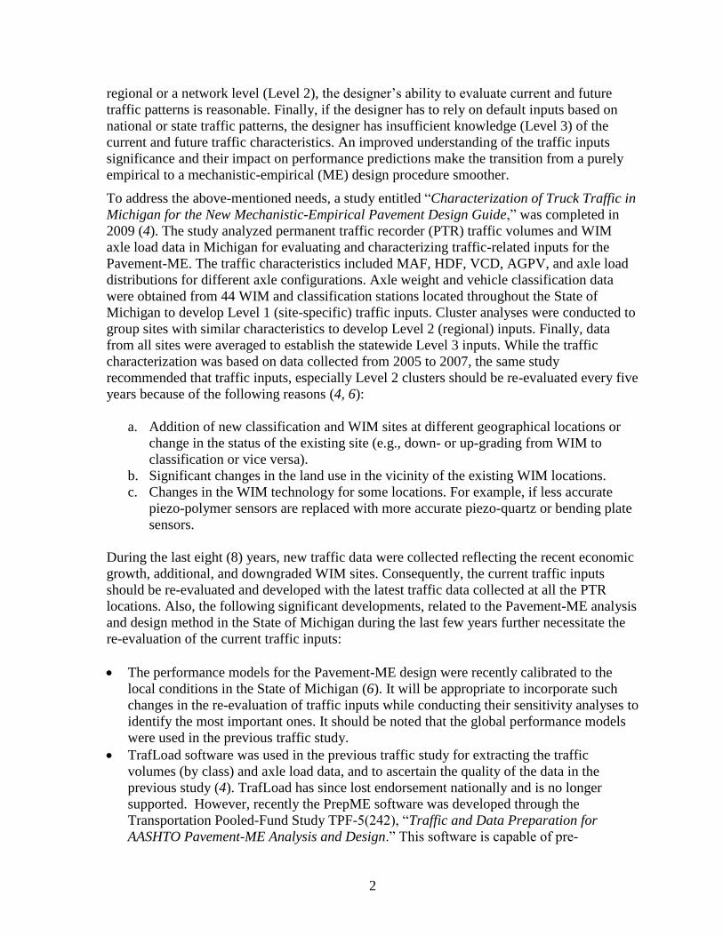
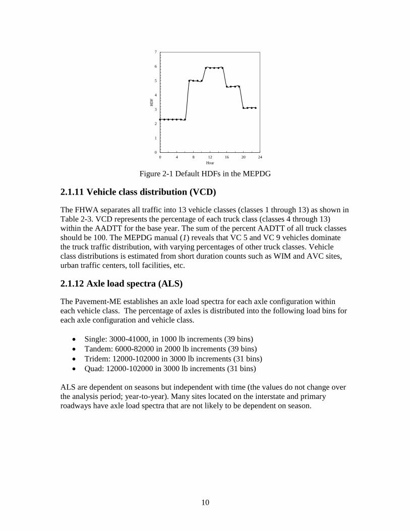
2.1.10 Hourly distribution factor (HDF)
HDFs establish the percentage AADTT that travels on the roadway for each of the 24
hours within a day. As most can relate to the increase of cars on the roadway during rush
hour, or peak hour, trucks also exhibit time-dependent behavior. Most hourly distribution
factors exhibit a trend of having a peak period between the hours of 10:00 am and 5:00
pm (6, 7). The TMG cites a study (5) in which trucking patterns were found to exhibit
two types of patterns. The first one being an almost constant percentage of trucks each
hour throughout the day and the other having a single-humped peak, typically during the
morning. The constant percentage trucks throughout the day signified a greater presence
of long-haul through trucks whereas the peaked distribution was found to be consistent
with local trucks (5). The default HDFs in the Pavement-ME are shown in Figure 2-1 and
the actual values by hours are shown in Table 2-2.
Table 2-2 The Pavement-ME default hourly distribution factors
Hour HDF Hour HDF
0 2.3 12 5.9
1 2.3 13 5.9
2 2.3 14 5.9
3 2.3 15 5.9
4 2.3 16 4.6
5 2.3 17 4.6
6 2.3 18 4.6
7 5 19 4.6
8 5 20 3.1
9 5 21 3.1
10 5 22 3.1
11 5.9 23 3.1
10
Figure 2-1 Default HDFs in the MEPDG
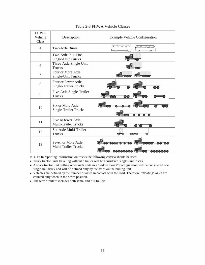
2.1.11 Vehicle class distribution (VCD)
The FHWA separates all traffic into 13 vehicle classes (classes 1 through 13) as shown in
Table 2-3. VCD represents the percentage of each truck class (classes 4 through 13)
within the AADTT for the base year. The sum of the percent AADTT of all truck classes
should be 100. The MEPDG manual (1) reveals that VC 5 and VC 9 vehicles dominate
the truck traffic distribution, with varying percentages of other truck classes. Vehicle
class distributions is estimated from short duration counts such as WIM and AVC sites,
urban traffic centers, toll facilities, etc.
2.1.12 Axle load spectra (ALS)
The Pavement-ME establishes an axle load spectra for each axle configuration within
each vehicle class. The percentage of axles is distributed into the following load bins for
each axle configuration and vehicle class.
Single: 3000-41000, in 1000 lb increments (39 bins)
Tandem: 6000-82000 in 2000 lb increments (39 bins)
Tridem: 12000-102000 in 3000 lb increments (31 bins)
Quad: 12000-102000 in 3000 lb increments (31 bins)
ALS are dependent on seasons but independent with time (the values do not change over
the analysis period; year-to-year). Many sites located on the interstate and primary
roadways have axle load spectra that are not likely to be dependent on season.
0
1
2
3
4
5
6
7
0 4 8 12 16 20 24
HD
F
Hour
11
Table 2-3 FHWA Vehicle Classes
FHWA
Vehicle
Class
Description Example Vehicle Configuration
4 Two-Axle Buses
5 Two-Axle, Six-Tire,
Single-Unit Trucks
6 Three-Axle Single-Unit
Trucks
7 Four or More Axle
Single-Unit Trucks
8 Four or Fewer Axle
Single-Trailer Trucks
9 Five-Axle Single-Trailer
Trucks
10 Six or More Axle
Single-Trailer Trucks
11 Five or fewer Axle
Multi-Trailer Trucks
12 Six-Axle Multi-Trailer
Trucks
13 Seven or More Axle
Multi-Trailer Trucks
NOTE: In reporting information on trucks the following criteria should be used:
Truck tractor units traveling without a trailer will be considered single-unit trucks.
A truck tractor unit pulling other such units in a "saddle mount" configuration will be considered one
single-unit truck and will be defined only by the axles on the pulling unit.
Vehicles are defined by the number of axles in contact with the road. Therefore, "floating" axles are
counted only when in the down position.
The term "trailer" includes both semi- and full trailers.
12
2.2 A REVIEW OF PREVIOUS STUDIES
Several research studies in the recent times focused on the following areas:
Analyzing Weigh-in-Motion (WIM), Automated Vehicle Classifier (AVC), and
automated traffic recorder (ATR) data with appropriate quality checks to develop
traffic inputs for the Pavement-ME.
Evaluating the effect of traffic inputs on the Pavement-ME distress predictions
and final pavement design thickness (sensitivity analysis).
Applying statistical models and techniques such as cluster analysis in identifying
homogenous traffic patterns.
Reviewing current traffic collection infrastructure and practices to meet the traffic
input requirements of the Pavement-ME.
The research team has found various guidelines, statistical models, and techniques used
to obtain the Levels 2 and 3 inputs for use in the Pavement-ME. Therefore, a review of
these studies has been conducted to study the application of different approaches in
traffic characterization. A summary of the review is presented below.
2.2.1 National Studies
Results of the research studies related to loading inputs (ALS) for use in the ME design
procedure are discussed in this section.
2.2.1.1 NCHRP 1-37A Study
The NCHRP 1-37A final report provides guidelines for truck traffic data collection for
both axle weights and truck volumes (8). These guidelines are based on the allowable
error and permissible bias for each data element in establishing the normalized truck
volume distribution and normalized axle load spectra (NALS). Truck traffic classification
(TTC) groups were developed based on the analysis of national WIM and AVC data
collected through the LTPP program. These TTC groups are used to characterize truck
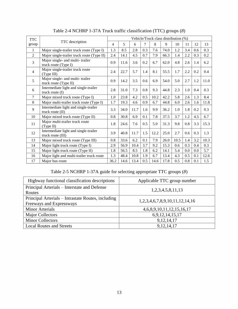
volume by vehicle class rather than by vehicle weight. Each TTC group represents a
traffic stream with unique truck traffic characteristics (see Table 2-4). For example, TTC
1 describes a traffic stream that is heavily populated with single-trailer trucks and TTC 17
contains more buses. A standardized set of TTC groups that best describes the traffic
stream for the different road functional classes is presented in Table 2-5. Table 2-6
presents the recommended data collection frequency for determining the TTC groups.
13
Table 2-4 NCHRP 1-37A Truck traffic classification (TTC) groups (8)
TTC
group TTC description
Vehicle/Truck class distribution (%)
4 5 6 7 8 9 10 11 12 13
1 Major single-trailer truck route (Type I) 1.3 8.5 2.8 0.3 7.6 74.0 1.2 3.4 0.6 0.3
2 Major single-trailer truck route (Type II) 2.4 14.1 4.5 0.7 7.9 66.3 1.4 2.2 0.3 0.2
3 Major single- and multi- trailer
truck route (Type I) 0.9 11.6 3.6 0.2 6.7 62.0 4.8 2.6 1.4 6.2
4 Major single-trailer truck route
(Type III) 2.4 22.7 5.7 1.4 8.1 55.5 1.7 2.2 0.2 0.4
5 Major single- and multi- trailer
truck route (Type II) 0.9 14.2 3.5 0.6 6.9 54.0 5.0 2.7 1.2 11.0
6 Intermediate light and single-trailer
truck route (I) 2.8 31.0 7.3 0.8 9.3 44.8 2.3 1.0 0.4 0.3
7 Major mixed truck route (Type I) 1.0 23.8 4.2 0.5 10.2 42.2 5.8 2.6 1.3 8.4
8 Major multi-trailer truck route (Type I) 1.7 19.3 4.6 0.9 6.7 44.8 6.0 2.6 1.6 11.8
9 Intermediate light and single-trailer
truck route (II) 3.3 34.0 11.7 1.6 9.9 36.2 1.0 1.8 0.2 0.3
10 Major mixed truck route (Type II) 0.8 30.8 6.9 0.1 7.8 37.5 3.7 1.2 4.5 6.7
11 Major multi-trailer truck route
(Type II) 1.8 24.6 7.6 0.5 5.0 31.3 9.8 0.8 3.3 15.3
12 Intermediate light and single-trailer
truck route (III) 3.9 40.8 11.7 1.5 12.2 25.0 2.7 0.6 0.3 1.3
13 Major mixed truck route (Type III) 0.8 33.6 6.2 0.1 7.9 26.0 10.5 1.4 3.2 10.3
14 Major light truck route (Type I) 2.9 56.9 10.4 3.7 9.2 15.3 0.6 0.3 0.4 0.3
15 Major light truck route (Type II) 1.8 56.5 8.5 1.8 6.2 14.1 5.4 0.0 0.0 5.7
16 Major light and multi-trailer truck route 1.3 48.4 10.8 1.9 6.7 13.4 4.3 0.5 0.1 12.6
17 Major bus route 36.2 14.6 13.4 0.5 14.6 17.8 0.5 0.8 0.1 1.5
Table 2-5 NCHRP 1-37A guide for selecting appropriate TTC groups (8)
Highway functional classification descriptions Applicable TTC group number
Principal Arterials – Interstate and Defense
Routes 1,2,3,4,5,8,11,13
Principal Arterials – Intrastate Routes, including
Freeways and Expressways 1,2,3,4,6,7,8,9,10,11,12,14,16
Minor Arterials 4,6,8,9,10,11,12,15,16,17
Major Collectors 6,9,12,14,15,17
Minor Collectors 9,12,14,17
Local Routes and Streets 9,12,14,17
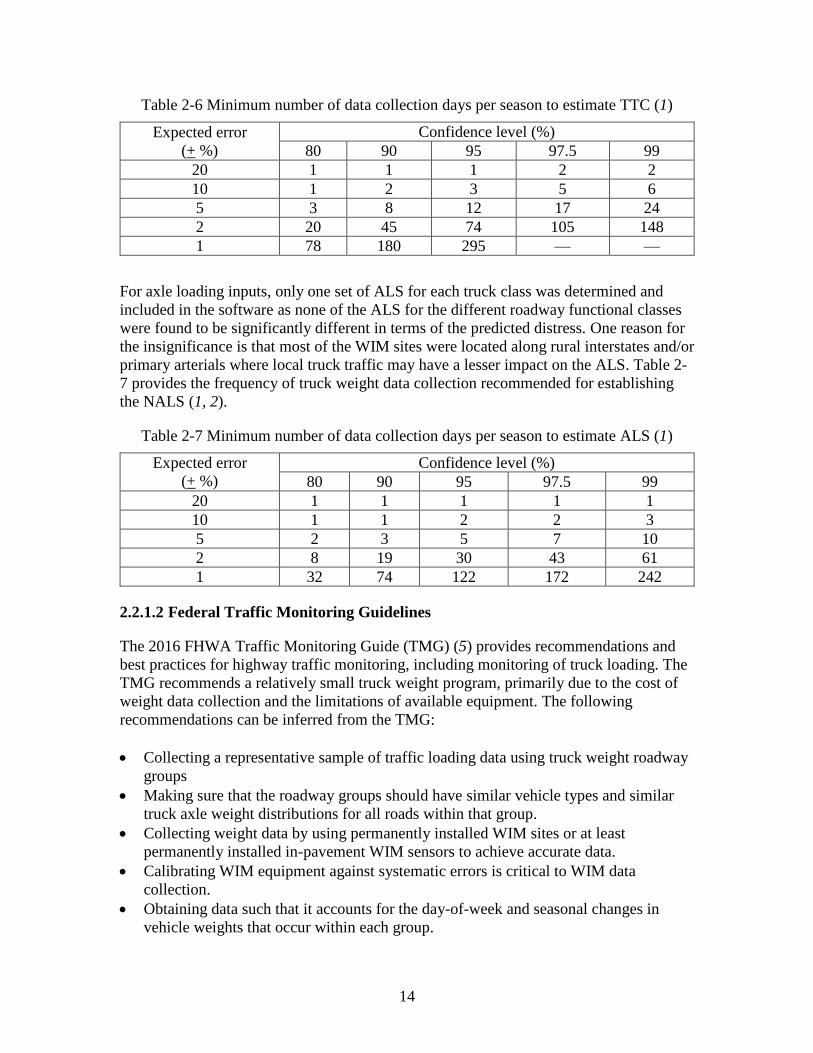
14
Table 2-6 Minimum number of data collection days per season to estimate TTC (1)
Expected error
(+ %)
Confidence level (%)
80 90 95 97.5 99
20 1 1 1 2 2
10 1 2 3 5 6
5 3 8 12 17 24
2 20 45 74 105 148
1 78 180 295 — —
For axle loading inputs, only one set of ALS for each truck class was determined and
included in the software as none of the ALS for the different roadway functional classes
were found to be significantly different in terms of the predicted distress. One reason for
the insignificance is that most of the WIM sites were located along rural interstates and/or
primary arterials where local truck traffic may have a lesser impact on the ALS. Table 2-
7 provides the frequency of truck weight data collection recommended for establishing
the NALS (1, 2).
Table 2-7 Minimum number of data collection days per season to estimate ALS (1)
Expected error
(+ %)
Confidence level (%)
80 90 95 97.5 99
20 1 1 1 1 1
10 1 1 2 2 3
5 2 3 5 7 10
2 8 19 30 43 61
1 32 74 122 172 242
2.2.1.2 Federal Traffic Monitoring Guidelines
The 2016 FHWA Traffic Monitoring Guide (TMG) (5) provides recommendations and
best practices for highway traffic monitoring, including monitoring of truck loading. The
TMG recommends a relatively small truck weight program, primarily due to the cost of
weight data collection and the limitations of available equipment. The following
recommendations can be inferred from the TMG:
Collecting a representative sample of traffic loading data using truck weight roadway
groups
Making sure that the roadway groups should have similar vehicle types and similar
truck axle weight distributions for all roads within that group.
Collecting weight data by using permanently installed WIM sites or at least
permanently installed in-pavement WIM sensors to achieve accurate data.
Calibrating WIM equipment against systematic errors is critical to WIM data
collection.
Obtaining data such that it accounts for the day-of-week and seasonal changes in
vehicle weights that occur within each group.

15
The truck traffic may vary significantly within a state depending on the road and land
use. The roadway system could be divided into roadway groups such that each road
within a group experiences similar truck-loading patterns. These groups may be defined
based on different methods, such as statistical analysis, a professional judgment based on
local knowledge of loading characteristics, or a combination of both. Characteristics of
the freight moved on the roads, including the type of commodities carried, the vehicles
used, and the freight movement could be used for dividing the roadway system (5). The
developed roadway groups should be simple enough and logical in discriminating roads
that are likely to have different traffic loading patterns.
The developed roadway groups should be periodically reviewed as more traffic data
within the state becomes available over time. The accuracy of these road groups depends
on the accuracy and precision of the collected weight data. Also, the more data collection
sites within a roadway groups, the higher will be the confidence level in the traffic inputs
generated. A minimum of six WIM sites with permanently installed WIM sensors per
truck weight group is recommended (5).
2.2.1.3 NCHRP 1-39 Guidelines
The NCHRP 1-39 report (9) contains guidelines for collecting traffic data to be used in
mechanistic-empirical pavement design. Three levels of axle-load distribution (or “load
spectra”) data are needed for the Pavement-ME: (a) site-specific, (b) TWRG, and (c)
statewide averages. Site-specific data requires an adequately calibrated WIM system and
near the roadway segment to be constructed or rehabilitated. If the WIM system is
unavailable or not properly calibrated (according to the ASTM requirements), Level 2
design inputs should be used to characterize traffic for design.
TWRG axle-loading data are needed because most States do not have sufficient site-
specific WIM data for the majority of pavements they design each year. The TWRGs are
likely to be state-specific, but multiple states can create “regional” axle load distribution
values if these States have similar truck weight laws and enforcement programs. The
intent is to group roads by their trucking characteristics so that the load spectra on all the
roads in a group are similar. The challenge is to determine the roads (and directions of
travel, in some cases) to choose for grouping. The grouping process requires analysis of a
State’s available weight data and trucking patterns, possibly for different truck classes,
and it results in the creation of appropriate TWRGs. Roadways with similar truck classes
may carry different loads. For example, a single road could have loaded trucks in one
direction and unloaded trucks in the other direction resulting in two TWRGs needed to
characterize axle load distributions for that road.
Also, it was reported that the simple averages of the load distribution at all sites in a
TWRG produced better results than weighted averages. It is attributed to a significant
positive correlation between the volume of trucks in a particular vehicle class operating at
a site and the average loads of these trucks. Because of this correlation, weighted
averages produced higher estimates of average pavement load per vehicle than simple
averages.
16
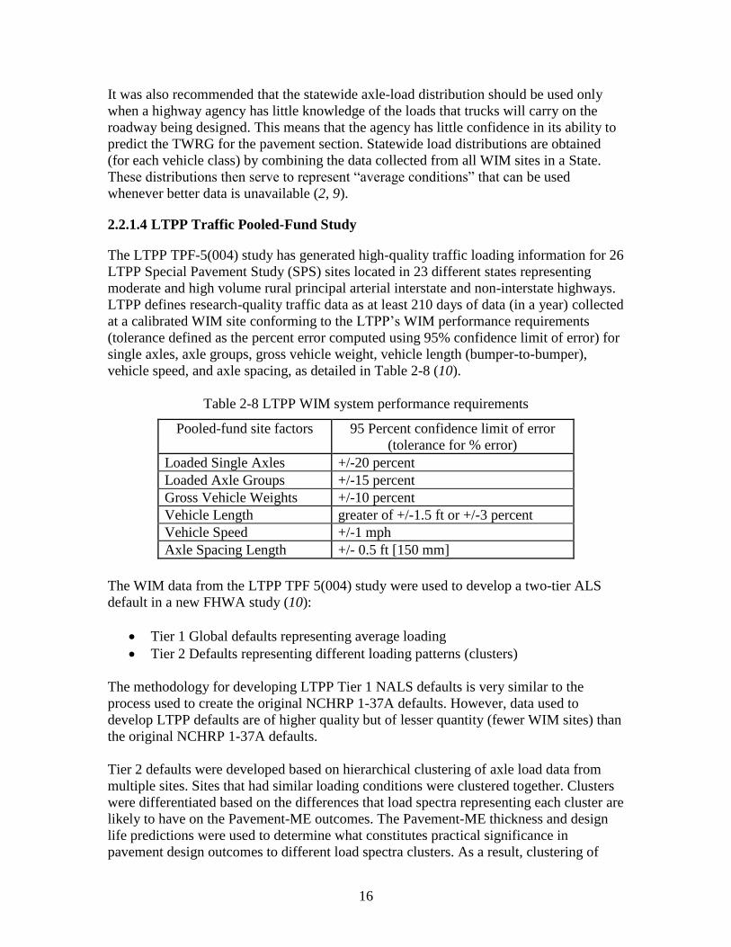
It was also recommended that the statewide axle-load distribution should be used only
when a highway agency has little knowledge of the loads that trucks will carry on the
roadway being designed. This means that the agency has little confidence in its ability to
predict the TWRG for the pavement section. Statewide load distributions are obtained
(for each vehicle class) by combining the data collected from all WIM sites in a State.
These distributions then serve to represent “average conditions” that can be used
whenever better data is unavailable (2, 9).
2.2.1.4 LTPP Traffic Pooled-Fund Study
The LTPP TPF-5(004) study has generated high-quality traffic loading information for 26
LTPP Special Pavement Study (SPS) sites located in 23 different states representing
moderate and high volume rural principal arterial interstate and non-interstate highways.
LTPP defines research-quality traffic data as at least 210 days of data (in a year) collected
at a calibrated WIM site conforming to the LTPP’s WIM performance requirements
(tolerance defined as the percent error computed using 95% confidence limit of error) for
single axles, axle groups, gross vehicle weight, vehicle length (bumper-to-bumper),
vehicle speed, and axle spacing, as detailed in Table 2-8 (10).
Table 2-8 LTPP WIM system performance requirements
Pooled-fund site factors 95 Percent confidence limit of error
(tolerance for % error)
Loaded Single Axles +/-20 percent
Loaded Axle Groups +/-15 percent
Gross Vehicle Weights +/-10 percent
Vehicle Length greater of +/-1.5 ft or +/-3 percent
Vehicle Speed +/-1 mph
Axle Spacing Length +/- 0.5 ft [150 mm]
The WIM data from the LTPP TPF 5(004) study were used to develop a two-tier ALS
default in a new FHWA study (10):
Tier 1 Global defaults representing average loading
Tier 2 Defaults representing different loading patterns (clusters)
The methodology for developing LTPP Tier 1 NALS defaults is very similar to the
process used to create the original NCHRP 1-37A defaults. However, data used to
develop LTPP defaults are of higher quality but of lesser quantity (fewer WIM sites) than
the original NCHRP 1-37A defaults.
Tier 2 defaults were developed based on hierarchical clustering of axle load data from
multiple sites. Sites that had similar loading conditions were clustered together. Clusters
were differentiated based on the differences that load spectra representing each cluster are
likely to have on the Pavement-ME outcomes. The Pavement-ME thickness and design
life predictions were used to determine what constitutes practical significance in
pavement design outcomes to different load spectra clusters. As a result, clustering of
17
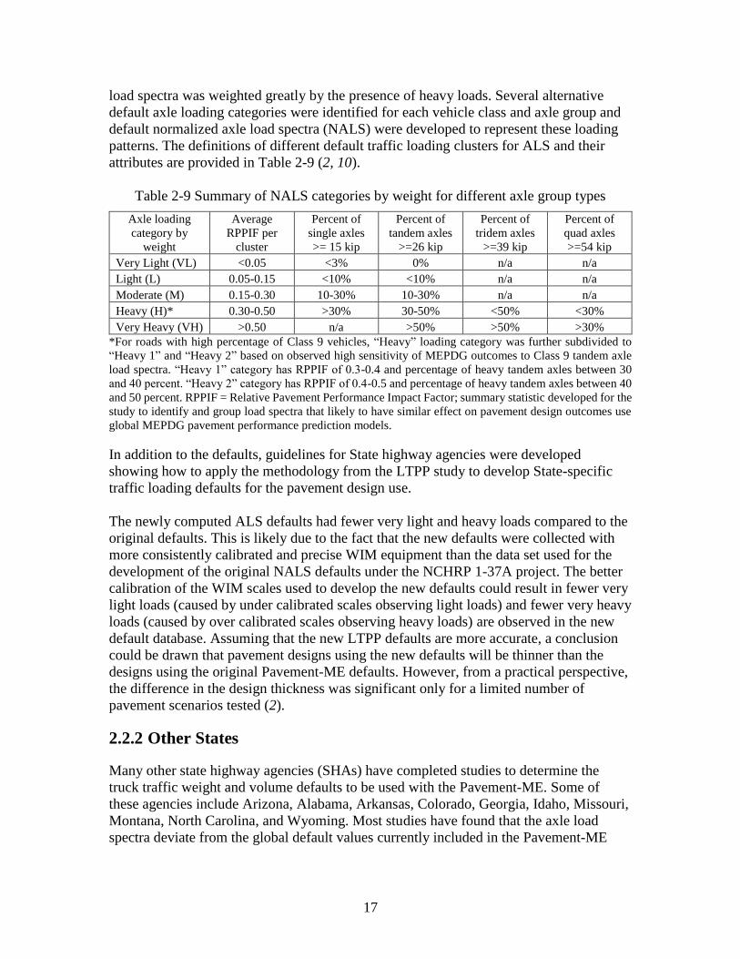
load spectra was weighted greatly by the presence of heavy loads. Several alternative
default axle loading categories were identified for each vehicle class and axle group and
default normalized axle load spectra (NALS) were developed to represent these loading
patterns. The definitions of different default traffic loading clusters for ALS and their
attributes are provided in Table 2-9 (2, 10).
Table 2-9 Summary of NALS categories by weight for different axle group types
Axle loading
category by
weight
Average
RPPIF per
cluster
Percent of
single axles
>= 15 kip
Percent of
tandem axles
>=26 kip
Percent of
tridem axles
>=39 kip
Percent of
quad axles
>=54 kip
Very Light (VL) <0.05 <3% 0% n/a n/a
Light (L) 0.05-0.15 <10% <10% n/a n/a
Moderate (M) 0.15-0.30 10-30% 10-30% n/a n/a
Heavy (H)* 0.30-0.50 >30% 30-50% <50% <30%
Very Heavy (VH) >0.50 n/a >50% >50% >30%
*For roads with high percentage of Class 9 vehicles, “Heavy” loading category was further subdivided to
“Heavy 1” and “Heavy 2” based on observed high sensitivity of MEPDG outcomes to Class 9 tandem axle
load spectra. “Heavy 1” category has RPPIF of 0.3-0.4 and percentage of heavy tandem axles between 30
and 40 percent. “Heavy 2” category has RPPIF of 0.4-0.5 and percentage of heavy tandem axles between 40
and 50 percent. RPPIF = Relative Pavement Performance Impact Factor; summary statistic developed for the
study to identify and group load spectra that likely to have similar effect on pavement design outcomes use
global MEPDG pavement performance prediction models.
In addition to the defaults, guidelines for State highway agencies were developed
showing how to apply the methodology from the LTPP study to develop State-specific
traffic loading defaults for the pavement design use.
The newly computed ALS defaults had fewer very light and heavy loads compared to the
original defaults. This is likely due to the fact that the new defaults were collected with
more consistently calibrated and precise WIM equipment than the data set used for the
development of the original NALS defaults under the NCHRP 1-37A project. The better
calibration of the WIM scales used to develop the new defaults could result in fewer very
light loads (caused by under calibrated scales observing light loads) and fewer very heavy
loads (caused by over calibrated scales observing heavy loads) are observed in the new
default database. Assuming that the new LTPP defaults are more accurate, a conclusion
could be drawn that pavement designs using the new defaults will be thinner than the
designs using the original Pavement-ME defaults. However, from a practical perspective,
the difference in the design thickness was significant only for a limited number of
pavement scenarios tested (2).
2.2.2 Other States
Many other state highway agencies (SHAs) have completed studies to determine the
truck traffic weight and volume defaults to be used with the Pavement-ME. Some of
these agencies include Arizona, Alabama, Arkansas, Colorado, Georgia, Idaho, Missouri,
Montana, North Carolina, and Wyoming. Most studies have found that the axle load
spectra deviate from the global default values currently included in the Pavement-ME

18
software, especially for local and secondary routes. Thus, the axle load spectra or
distributions can depend on the roadway use and/or geographical location.
2.2.2.1 Arizona
A research study (11) sponsored by the Arizona Department of Transportation (ADOT)
addressed the collection, preparation, and use of traffic data required for pavement
design. Procedures to collect Level 1 traffic inputs were documented. Levels 2 and 3
recommended inputs and defaults are provided based on the best historical data available
to date using multivariate hierarchical statistical cluster analyses (using correlation
coefficient (R2) method)(11). Although determining the optimum number of clusters
within a dataset is a subjective decision, five diagnostic statistics were used for
determining the optimum number of clusters. Those were (a) Cubic clustering criterion
(CCC), (b) Cumulative and partial squared multiple correlations (R2), (c) Eigenvalue and
associated variance (VAR), (d) Pseudo F (PSF) and (e) Pseudo t2 (PST2). Based on the
clustering and sensitivity analyses, two clusters for vehicle class distribution, two clusters
for hourly distribution factors, one cluster for monthly distribution factor, three clusters
for axle load distribution, and one cluster for axles per truck were recommended. The
selection criteria of clusters are based on the highway functional classes (11).
2.2.2.2 Alabama
A study (12) was conducted in the State of Alabama to develop traffic data clusters for
use as inputs in the Pavement-ME. While the Pavement-ME requires only three input
levels, the second level inputs were further split into two subcategories in this study. The
levels considered were: (a) Level 1 – Site and direction specific data, (b) Level 2A –
Cluster or WIM group data, (c) Level 2B – Statewide data and (d) Level 3 – Nationwide
data. Thirteen types of traffic inputs were identified based on the Michigan study (13)
and clusters were developed for those inputs. Those 13 inputs are: 1 HDF, 1 VCD, 4
AGPV (single, tandem, tridem and quad), 3 MDF (single unit, tractor trailer and multi-
trailer) and 4 ALS (single, tandem, tridem and quad).
It was noted in the study that hierarchical cluster analysis was the most popular clustering
technique. Citing the disadvantages of using Euclidean distance, which is state of the
practice, the researchers used Pearson’s correlation coefficient (𝑟𝑗k) for clustering
purposes. Also, a correlation-based clustering that combines Pearson’s correlation
distance measure (to evaluate similarity) with unweighted pair group method using
arithmetic averages (UPGMA) (to cluster WIM sites) was developed in this study. Once
the clusters were developed, sensitivity analyses were conducted to quantify the
differences in required pavement thickness between different traffic inputs levels.
Geographical patterns were defined to assist in selecting the appropriate clusters for new
pavement design (12).
2.2.2.3 Arkansas
Another study conducted in the State of Arkansas analyzed WIM data by using cluster
analysis methodologies to identify groups of WIM sites with similar traffic characteristics
19
based on the required traffic attributes (14). The research team normalized the traffic data
attributes on an annual basis. Ten WIM sites located in Arkansas which passed the truck
weigh data quality check process have been used in the analyses. Ward’s minimum-
variance method was used. A dissimilarity coefficient matrix based on the Euclidean
distance for each pair of objects was computed for the 10 WIM sites. Three clusters were
identified when distribution of gross weight of Class 9 truck was used as the attribute.
Two other clustering approaches, K-mean and fuzzy cluster analyses were also applied to
the data for comparison purposes. The classifications of clusters had little differences
among these three approaches used indicating the patterns of the traffic stream were
consistent regardless of cluster methodologies. The clusters for vehicle class distribution
factors (VCDs), hourly distribution factors (HDFs), and monthly adjustment factors
(MAFs) were identified by using the K-means clustering procedure. Three clusters for
vehicle class distributions and monthly adjustment factors, and two clusters for hourly
distribution factors were observed. Grouping based on a combination of known
geographic, industrial, agricultural, and commercial patterns was done using the Fisher’s
Exact Test (15) for developing the loading groups. Categorical statistical models (multi-
category logit [ML] models) were developed to assign a new pavement design project to
a cluster (14).
2.2.2.4 Colorado
A study was conducted in Colorado with the main objectives being (1) determine how
representative available traffic data are for pavement design in Colorado using the
Pavement-ME, (2) detect natural groupings or clusters within the available traffic data,
and (3) develop defaults for Levels 2 and 3 traffic inputs for pavement design (16).
Statistical analysis to determine natural clusters within the traffic and the optimum
number of clusters was conducted. Natural clusters within the large Colorado traffic data
assembled were determined using statistical multivariate hierarchical cluster analysis
similar to the analysis done in the State of Arizona (11). Clusters were formed for vehicle
class distribution, hourly truck volume distribution, monthly adjustment factors, axles per
truck class factors, axle load distribution.
2.2.2.5 North Carolina
North Carolina Department of Transportation (NCDOT) sponsored a study for the
implementation of the Pavement-ME in the State of North Carolina (17). The study
included developing the need for resources, procedures, and guidelines for NCDOT
traffic data needed for the Pavement-ME. Clustering analyses was performed to develop
the required traffic inputs. Initial clustering analysis of 42 WIM sites based on VCD for
different months resulted in three major clusters or factor groups. Each factor group
includes WIM sites that tend to remain in same cluster over the year (from January to
December).
Even though the cluster analyses led to different clusters, the pavement performance was
found to be insensitive to hourly distribution factors and monthly adjustment factors.
Hence state wide averages were recommended for use. Multi-dimensional clustering was
used to determine the Level 2 inputs for axle load spectra. Multi-dimensional clustering
20
tests the similarity among WIM data based on several attributes, where one dimensional
clustering does it based on one attribute at a time. One dimensional analysis provides
clusters which are distinct by one axle type, but they are difficult to interpret or relate to a
definite traffic pattern. Therefore, the cluster representing single axles may not contain
the characteristics of roadways where tandem axles are predominant. Moreover, Class 5
(two single axles) and Class 9 (one single axle and two tandem axles) are the
predominant truck classes in North Carolina. Class 5 and 9 represented single and tandem
axles better, respectively (18). Thus, the implementation of multi-dimensional (two-
dimensional clustering using Ward’s method) clustering may improve the results,
because it considers the relationship of multiple attributes simultaneously and processes
well-explained clusters. For new pavement projects, 48-hour site specific classification
counts were used to derive the traffic parameters (17).
2.2.2.6 New York
A study was performed to characterize the traffic inputs (VCD, MDF, HDF, AGPV, and
axle load spectra) for the State of New York. Data were obtained from vehicle
classification and WIM sites in New York during years 2007 to 2011. Cluster analysis
was performed only for VCD, MDF, and HDF due to the unavailability of data for a
sufficient number of WIM sites. The MEPDG analyses were executed to study the effect
on predicted pavement performance using site-specific, regional (clusters), statewide
average and the MEPDG default values on predicted performance measures for
conventional new flexible and rigid pavement structures. Ward’s method of cluster
analysis was adopted. Semi-partial R-squared (SPR) values were used to determine the
number of clusters to be selected for further analyses.
Four clusters were formed for the vehicle classification distribution (VCD). Those are
differentiated based on proportions of Class 5 and Class 9 vehicles. The direction of
travel has little impact on the VCD. The results of cluster analysis are consistent for all
the years. Multi-dimensional clustering was adopted for monthly distribution factors
considering Class 5 and 9 vehicles simultaneously. Four clusters were formed for 2007,
2008 and 2010. However, three and five clusters were formed for 2009 and 2010
respectively. Four clusters are found for hourly distribution factors for each of the years.
The results of cluster analysis are almost consistent over the years. HDF does not show
any impact on the performances of pavement. The study recommends statewide average
values for VCD, MDF, AGPV, and ALS.
2.2.2.7 Georgia
A study was conducted to make recommendations for establishing Georgia Department
of Transportation (GDOT) traffic load spectra program and the WIM data collection plan
to support the implementation of the Pavement-ME analysis and design (2). There are
very few permanent WIM sites in the State of Georgia, and the data obtained from the
portable WIM sites were considered inadequate as a Level 1 input. It was mainly due to
the limitation of equipment accuracy and challenges with field calibration of the portable
WIM system. GDOT’s vehicle classification data from automated vehicle classification
(AVC) sites were also reviewed and categorized by the MEPDG truck traffic
21
classification (TTC) groups by the researchers. Not all default MEPDG TTCs were
observed in Georgia. The study recommended that NALS defaults developed as part of
the FHWA study (10) be used until more Georgia permanent WIM data become available
to compute Georgia-specific loading defaults. This recommendation was based on
similarities in loading characteristics and the Pavement-ME outcomes using Georgia
WIM data and LTPP defaults. For new alignments, it was recommended that the new
NALS be based on the type of traffic loading condition expected based on aggregated
road functional classes, GA freight route designation, and expected AADTT and percent
of class 9 vehicles A decision tree based on these factors was developed to assist the
pavement designers.
2.2.2.8 Idaho
Site-specific traffic inputs were developed based on the analyses of traffic data from 12
out of 25 WIM sites in Idaho as part of the States’ MEPDG implementation effort.
Statewide axle load spectra and an average number of axles per truck were established.
The significance of the MEPDG predicted performance in relation to axle load spectra,
vehicle class distribution, monthly adjustment factors and an average number of axle per
truck was also investigated. The results showed an average directional distribution, and
lane distribution factors agree quite well with the MEPDG recommended default values.
Also, in general, Class 9 followed by Class 5 trucks represented the majority of the trucks
traveling on Idaho roads. The vehicle class distribution factors at 5 out of 12 investigated
WIM sites did not match any of the MEPDG recommended TTC groups. The developed
MAF ranged between 0 and 4 indicating that truck volumes vary from month to month.
The peak locations of the developed statewide and the MEPDG default ALS were fairly
similar for the majority of the truck classes and axle types. However, the percentages of
axles within these peaks were different, especially for the tridem and quad axles(19). The
number of single, tandem and tridem axles per truck for all truck classes based on Idaho
data was found quite similar to the MEPDG default values. Idaho data showed few
percentages of quad axles for truck classes 7, 10, 11, and 13 compared to the MEPDG
default values which are all zero.
The developed statewide axle load spectra yielded significantly higher longitudinal and
alligator cracking compared to the MEPDG default spectra. No significant differences
were observed for predicted AC rutting, total rutting, and IRI based on statewide and the
MEPDG default spectra. High prediction errors were found for longitudinal cracking
when statewide/national (Level 3) axle load spectra, vehicle class distribution, or monthly
adjustment factors were used instead of site-specific (Level 1) data. Large prediction
errors in alligator cracking were only found when the statewide default axle load spectra
were used compared to site-specific spectra. Moderate errors were found when the
MEPDG typical default monthly adjustment factors or vehicle class distribution were
used instead of the site-specific values. The input level of the axle load spectra, monthly
adjustment factors, vehicle class distribution, and number of axles per truck had very low
impact on predicted AC rutting and negligible impact on total rutting and IRI. The input
level of the number of axles per truck had negligible influence on the MEPDG predicted
performance. (19)
22
2.3 REVIEW OF EXISTING PRACTICES IN MICHIGAN
The final report “Characterization of Truck Traffic in Michigan for the New Mechanistic-
Empirical Pavement Design Guide” was reviewed to determine if the clustering
methodology used in the 2009 study is still the “best” way for MDOT to develop Levels
2 and 3 inputs for the Pavement-ME use. Another goal of the review was to determine if
the current methodology could be improved or simplified to address the needs and
constraints faced by MDOT traffic data personnel. In making this determination,
techniques used by other SHAs to accomplish similar task were considered.
Several statistical techniques were used in the 2009 study to develop and test traffic
clusters and default values. Also, the MEPDG sensitivity analyses were conducted to test
the clusters and recommendations on the use of Level 2 (cluster-based) and Level 3
(statewide) defaults were included. Implementation of this approach could be further
improved in several areas, as described below.
2.3.1 Potential Areas of Improvement in the Current Practices
Several areas were identified during the review that would benefit from revisions and
would lead to the development of the improved road groupings or clusters for the
determining more representative Level 2 and Level 3 traffic defaults. The following
potential improvements are proposed in the current methodology:
1. Level 3 defaults represent statewide traffic conditions, as such the data from traffic
sites used to develop these defaults should be representative of all the State roads that
may be designed using the Pavement-ME. Having sample skewed towards a specific
road type (that has a disproportionately higher representation in the sample) may bias
the statewide defaults. Traffic characteristics on interstate roads and high heavy truck
volume primary arterial non-interstate roads typically differ from those observed on
non-interstate low heavy truck volume roads. It may be beneficial to have two
statewide defaults: one for interstate and high heavy truck volume roads (i.e.,
designated state freight routes) and another for all other roads. Such strategy would
also reduce bias towards a particular road type and account for potential future
changes in traffic characteristics or pavement design requirements for these types of
roads.
2. In the 2009 study, the term TTC was used both to define cluster groups and as a name
of vehicle class distribution input. While TTC is an appropriate name for road clusters
that show specific truck traffic characteristics (hence, TTC term), the term ‘VCD’
could be used to refer to the Pavement-ME vehicle class distribution input.
3. The three VCD clusters developed were not clearly defined in terms of available non-
vehicle classification parameters such as road class (i.e., freeway and non-freeway).
This poses some challenges for assigning a particular cluster default to a site without
site-specific data.
4. An alternative approach to clustering could be used to study similarities in VCD and
AADTT levels within road functional classes and then develop clusters based on
aggregated functional classes, using AADTT as a secondary qualifier. Clusters or
groups based on this approach would allow easy assignment of TTC defaults, as well
23
as easy updates of Level 2 defaults in the future. Effect of this simplified approach
could be further evaluated using the Pavement-ME sensitivity results.
5. When developing monthly distribution factors, vehicle classes were divided into three
groups based on body type: VC 4-7, VC 8-10, and VC 11-13 (i.e., single-unit, tractor-
trailer combination, and multi-trailer combination). Insignificant seasonal variations
were observed in the data. This could be due to the fact that vehicles that serve unlike
purposes were combined in the same group (local service trucks or resource-
extraction industry trucks were combine with long-haul trucks). Therefore, there is a
need to determine Level 2 inputs based on the most observed VCs in Michigan (i.e.,
VC5 and VC9).
6. The 2009 report identified differences in single, tandem, tridem, and quad axles per
vehicle group (AGPV) values. AGPVs are typically stable between the roads unless
some unusual truck fleets are using these roads. AGPV is a function of the truck fleet,
not road or location. Significant deviations in AGPV could be a sign of vehicle
misclassification. The reason is attributed to misclassification of vehicles by Trafload
software. It is expected that no difference in AGPV should be observed with the
PrepME.
7. In the 2009 study, the single axle load spectra were grouped into three clusters. The
clustering was based on VC5 and VC9 percentages and was not based on axle weight
differences on the truck-level. Differences in axle weights should be used for
individual truck classes. When axle load spectrum is based on all classes combined,
then proportion of light weight vehicle classes to heavy weight vehicle classes (i.e.
the proportion of VC5 and VC9 vehicles) matters more than truck weight
characteristics of a given vehicle class. Since another parameter - VCD parameter is
already being used by the MEPDG method to account for proportion of different
vehicle classes, there is no need to account for that again in clustering of axle load
spectra. Instead, it would be of an advantage to figure out which roads have high
percentage of light or heavily loaded trucks for individual vehicle classes that are
dominant on Michigan roads (i.e., focus on identifying roads that has a lot of empty
or fully loaded freight trucks or empty/loaded service trucks, or empty/loaded
resource extraction trucks).
8. The tandem axle load spectra were developed based on all vehicle classes combined.
These spectra exhibited five distinct clusters. Clusters 1-3 showed the presence of
lighter axles as compared to Clusters 4 and 5. Dominant truck classes with tandem
axles (typically VC8 and VC9) should be focused on for developing Level 2 inputs.
9. In tandem clusters, the loaded peak was reported in 30-35 kips range. With a legal
load limit of 34 kip, 35 kip peak seems to be a sign of low precision or calibration
drift. Data quality issues should be further investigated using new data. Information
about calibration frequency, procedures, and documented accuracy are essential in
concluding about data accuracy and precision.
10. The study indicated peak values for the quad axle load spectra occur at 104 kips. This
is an unexpected and unreasonable number that needs further investigation. Perhaps
these numbers manifest a catch-all function for penta+ (five or more) axles in the
TrafLoad software. If proven to be true, this would make sense. Penta+ axles should
be accounted for but not combined with quad axle load spectra. The PrepME should
be able to identify such axle configurations.

24
11. While the methodology used to develop clusters is well described, no step-by-step
procedures are provided in the report that could be used by MDOT to implement this
methodology. If clustering methodology was implemented in the PrepME software,
software algorithm should be documented in detail.
12. Review of the tandem, tridem, and quad loading defaults indicates potential data
anomalies, deviation from typical values, or issues with equipment precision and bias.
WIM calibration dates and calibration results should be used in WIM data QC
process to draw sound conclusions about data accuracy/reasonableness.
13. At least three years of data per vehicle class per site should be used to avoid
mistaking natural variations in truck volume (due to low volumes in some vehicle
classes) and identify repeatable and stable seasonal truck volume variations to
develop sound conclusions and defaults. Multiple years of WIM data will help to
reduce bias in measurements, effects of calibration drifts, as well as variations in
traffic.
14. In addition to the continuous data, data from short-term counts should be used to the
extent possible. Site-specific or site-related (same road, different location) 48-hour
vehicle classification count is better than Level 2 or 3 defaults, or at least it could be
used to guide the selection of the appropriate default. Such count could be obtained
inexpensively using pneumatic road tubes. It is likely that a significant amount of this
data is already available at MDOT and being collected annually as part of FHWA
HPMS data submission requirement.
15. For each road segment with site-specific traffic data, the available truck classification
and WIM data should be analyzed to identify “design lane” as a lane with the most
substantial number of heavy axle load applications. This information should be stored
in a database table for future use.
2.3.2 Recommended Improvements
Based on the review of other States’ ME implementation efforts and considering the
Pavement-ME requirements for traffic data characterization, several recommendations
for selecting, developing, or enhancing the existing methodology were developed, as
presented below.
1. The methodology should take into account pavement performance and pavement
design criteria used by MDOT. The number of traffic defaults should be determined
based on the differences in pavement design outcomes observed for a range of traffic
conditions identified from MDOT traffic data. If the differences in pavement design
outcomes are insignificant for the observed traffic conditions, one statewide default
would be sufficient. However, if pavement designs are sensitive to changes in the
traffic input parameters computed based the MDOT traffic data, then multiple traffic
defaults should be developed to represent each traffic loading condition that results in
different pavement design outcomes.
2. The methodology should be applicable for the roads that will be designed using the
Pavement-ME methodology, i.e., if multiple defaults are used, they should be
applicable to specific types of roads and pavements.

25
3. The methodology for the development of the defaults and the procedures for updating
the defaults or selecting defaults for specific pavement designs will be based on the
data that are readily available for MDOT personnel.
4. The methodology for axle load characterization and Level 2 grouping of roads should
focus on accurate characterization of loads that matter most for pavement designs
(i.e., heavy axle loads and dominant heavy truck classes).
5. The methodology for the development of the defaults and the procedures for updating
the defaults or selecting defaults for specific pavement designs should be well
documented and easy to follow. In other words, step-by-step instructions and
examples should be developed showing how to update the defaults, as well as how to
select and use the defaults in the pavement design.
6. The procedures for development, updating, and/or using defaults should be supported
by the tools available or developed for MDOT personnel.
7. The Pavement-ME Level 2 traffic inputs should be developed considering the
limitations of MDOT traffic data collection program. This primarily refers to the
limited number of continuous monitoring WIM and vehicle classification sites that
may not provide representative coverage of the roads in MI that will be designed
using the Pavement-ME. Also, due to unavailability of freight data for some routes.
8. Enhance WIM data QC checks from 2009 study to focus on the accuracy of heavy
loads and proper vehicle classification to compute site-specific parameters.
9. Use available MDOT traffic data to identify ranges of values for different traffic input
parameters, for different road functional classes:
Rural Interstates
Urban Interstates
Urban Freeway/Expressway and Non-Interstate Principal Arterials
Rural Non-Interstate Principal Arterials
All Minor Arterials and Collectors
10. Evaluate the practical significance of the findings, i.e., identify traffic parameters
where the use of multiple defaults would likely cause significant differences in
pavement design outcomes using criteria provided by MDOT (such as 3 or 4 years
difference in 20-year service life) using pavement ME locally-calibrated models.
Develop a list of parameters requiring Level 2 clusters.
11. Use functional road class, AADTT, and VCD information to see if these parameters
could be used to assign mathematical clustering results, i.e., find parameters that
could serve as cluster differentiators. If needed, introduce additional parameters that
are available to MDOT such as road type, the direction of travel, proximity, and size
of metropolitan areas, and freight route designation.
12. Once parameters that could characterize mathematical clusters are identified, develop
procedures showing how MDOT could use available information/parameters to
identify what cluster default to be used for the design. Develop decision trees or
automated procedures for MDOT to use in the cluster default selection process.
13. Develop procedures how cluster defaults could be updated in the future using
available cluster differentiators. In other words, use differentiators to identify and
assign available data for each “cluster” or group and compute average values for each

26
“cluster” to be used as new “cluster” defaults (no mathematical modeling should be
needed for this step).
14. Store computed site-specific Pavement-ME traffic inputs, Level 2 and 3 defaults in a
database, along with the information about traffic sites used to develop these defaults,
including information about site location, road inventory information, data collection
period, data availability (number of days with data), WIM calibration dates and
performance parameters (accuracy of measurements). Develop documentation
explaining database table designs, data upload, and data retrieval procedures.
15. Develop step-by-step instructions for MDOT pavement engineers for obtaining Level
2 traffic inputs for pavement design projects.
2.4 METHODOLGIES FOR DEVELOPING TRAFFIC INPUTS IN
MICHIGAN
Based on the above review, the following approaches are proposed for developing traffic
inputs in Michigan:
1. Improved existing methodology
2. Alternative simplified methodology
The following sections describe the summary of each proposed approach.
2.4.1 Improved Existing Methodology
Based on the review, several improvements are recommended to enhance the existing
methodology to characterize the traffic inputs based on the new (2011 to 2015) WIM and
classification data. Several areas were identified during the review that would lead to the
improved road groupings or clusters for more representative Level 2 and Level 3 defaults.
The following potential improvements are proposed in the current methodology:
1. Level 3 statewide defaults – Based on the distribution of PTR locations, it may be
beneficial to have 2 statewide defaults: one for interstates and roads with high volume
of heavy trucks (i.e. designated state freight routes) and one for all other roads.
2. Level 2 MAF groups/clusters – In the previous study, vehicle classes were divided
into three groups based on body type: VC 4-7, VC 8-10, and VC 11-13 (i.e., single-
unit, tractor-trailer combination, and multi-trailer combination). Very little seasonal
variations were observed. This could be due to the fact that different truck classes
were combined in the same group (i.e., local service trucks or resource-extraction
industry trucks were grouped with long-haul trucks). Analysis of individual vehicle
classes may help to better identify seasonal trends. This would be most applicable to
the vehicle classes that are frequently observed on MI roads (typically classes 5 and
9).
3. An easy to follow step-by-step procedure will be developed for future use by MDOT
personnel.
4. The current methodology uses freight data and discriminant analysis for assigning a
site to a cluster for significant traffic inputs. However, some routes do not have

27
freight data available. In such cases, there is a need to develop alternative approaches
to establish Level 2 traffic inputs for a particular project. For example, decision trees
based on the data availability can be developed and used for cluster assignments.
2.4.2 Alternative Simplified Methodology
The alternative simplified methodology will include the following steps:
1. Use available MDOT traffic data (AADTT, VCD information, and road
inventory/GIS information) to identify ranges of values for different traffic input
parameters for different road functional class groups, e.g.:
Rural interstates
Urban interstates
Urban freeway/expressway and non-interstate principal arterials
Rural non-interstate principal arterials
All minor arterials and collectors
2. If needed, introduce additional parameters that are available to MDOT such as road
type or designation (Interstate, US, State, county, etc.), direction of travel, proximity
and size of metropolitan areas, and freight route designation.
3. Once the groups are identified, establish the traffic inputs based on the averages of
sites in each individual group. Averages with these groups should be updated when a
PTR site is removed or added or new traffic data become available (see
recommendations in Chapter 6).
2.5 SUMMARY
This chapter presents a review of literature and state-of-the-practice related to traffic
inputs in the Pavement-ME. The Pavement-ME uses hierarchical input levels and
provides flexibility to the designer in obtaining the design inputs based on the project
importance. Three different input levels can be used in this hierarchical system ranging
from site-specific input values to “best-estimate” or default values as classified below:
1. Level 1 – These inputs provide the highest level of accuracy because they are
site/project specific and are measured directly,
2. Level 2 – These inputs provide an intermediate level of accuracy and are used
when Level 1 inputs are unavailable. Correlation or regression equations are used
to estimate these inputs.
3. Level 3 – These inputs are based on global or regional averages and provide the
least amount of knowledge regarding the input parameters.
Most of these inputs can be obtained through weigh-in-motion (WIM), automatic vehicle
classification (AVC), and vehicle counts, etc. Each of these traffic inputs were briefly
described in this chapter. Several guidelines used to obtain the Levels 2 and 3 inputs for
use in the Pavement-ME are documented. The NCHRP 1-37A final report (8) provides
guidelines for truck traffic data based on the allowable error and permissible bias for each

28
data element in establishing the truck volume distribution and axle load spectra. Also,
one set of ALS for each truck class was determined and included in the software as
defaults. The 2016 FHWA Traffic Monitoring Guide (TMG) (5) provides
recommendations and best practices for highway traffic monitoring, including monitoring
of truck loading. It is recommended that the roadway system be divided into groups using
clustering or traditional approaches such that each road within a group experiences
similar truck-loading patterns. The NCHRP 1-39 report (9) also contains guidelines for
collecting traffic data to be used in the MEPDG. The LTPP TPF-5(004) study has
generated high-quality traffic loading information for 26 LTPP Special Pavement Study
(SPS) sites located in 23 different States representing moderate and high volume rural
principal arterial interstate and non-interstate highways. The WIM data from the LTPP
TPF 5(004) study were used to develop a two-tier ALS defaults (10): (a) Tier 1 Global
defaults representing average loading, and (b) Tier 2 Defaults representing different
loading patterns (clusters). Tier 2 defaults were developed based on hierarchical
clustering of axle load data from multiple sites. The newly computed ALS defaults had
fewer very light and heavy loads compared to the original defaults. This is likely due to
the fact that the new defaults were collected with more consistently calibrated and precise
WIM equipment than the data set used for the development of the original NALS defaults
under the NCHRP 1-37A project.
Many other state highway agencies (SHAs) have determined the truck traffic weight and
volume defaults to be used with the Pavement-ME. It was found that that the local axle
load spectra for different axle configurations deviate from the global default values
currently included in the Pavement-ME software, especially for local and secondary
routes. Therefore, the development of regional or statewide traffic defaults is necessary to
implement the Pavement-ME design approach. Various approaches have been used to
obtain the Levels 2 and 3 inputs for use in the Pavement-ME. A review of these
techniques used by other States is provided in Table 2-10.
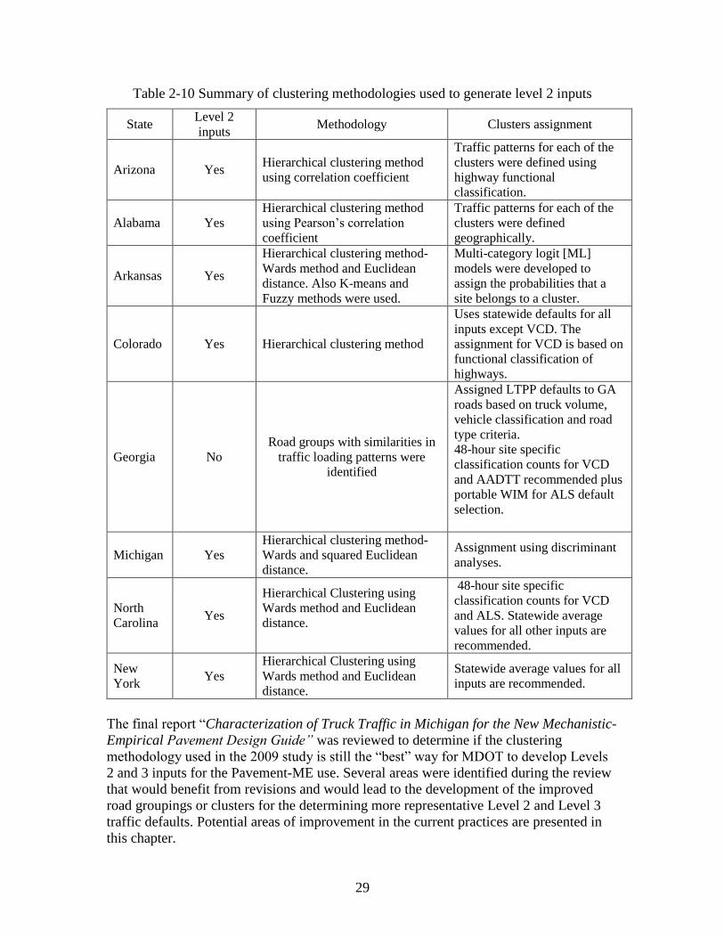
29
Table 2-10 Summary of clustering methodologies used to generate level 2 inputs
State Level 2
inputs Methodology Clusters assignment
Arizona Yes Hierarchical clustering method
using correlation coefficient
Traffic patterns for each of the
clusters were defined using
highway functional
classification.
Alabama Yes
Hierarchical clustering method
using Pearson’s correlation
coefficient
Traffic patterns for each of the
clusters were defined
geographically.
Arkansas Yes
Hierarchical clustering method-
Wards method and Euclidean
distance. Also K-means and
Fuzzy methods were used.
Multi-category logit [ML]
models were developed to
assign the probabilities that a
site belongs to a cluster.
Colorado Yes Hierarchical clustering method
Uses statewide defaults for all
inputs except VCD. The
assignment for VCD is based on
functional classification of
highways.
Georgia No
Road groups with similarities in
traffic loading patterns were
identified
Assigned LTPP defaults to GA
roads based on truck volume,
vehicle classification and road
type criteria.
48-hour site specific
classification counts for VCD
and AADTT recommended plus
portable WIM for ALS default
selection.
Michigan Yes
Hierarchical clustering method-
Wards and squared Euclidean
distance.
Assignment using discriminant
analyses.
North
Carolina Yes
Hierarchical Clustering using
Wards method and Euclidean
distance.
48-hour site specific
classification counts for VCD
and ALS. Statewide average
values for all other inputs are
recommended.
New
York Yes
Hierarchical Clustering using
Wards method and Euclidean
distance.
Statewide average values for all
inputs are recommended.
The final report “Characterization of Truck Traffic in Michigan for the New Mechanistic-
Empirical Pavement Design Guide” was reviewed to determine if the clustering
methodology used in the 2009 study is still the “best” way for MDOT to develop Levels
2 and 3 inputs for the Pavement-ME use. Several areas were identified during the review
that would benefit from revisions and would lead to the development of the improved
road groupings or clusters for the determining more representative Level 2 and Level 3
traffic defaults. Potential areas of improvement in the current practices are presented in
this chapter.
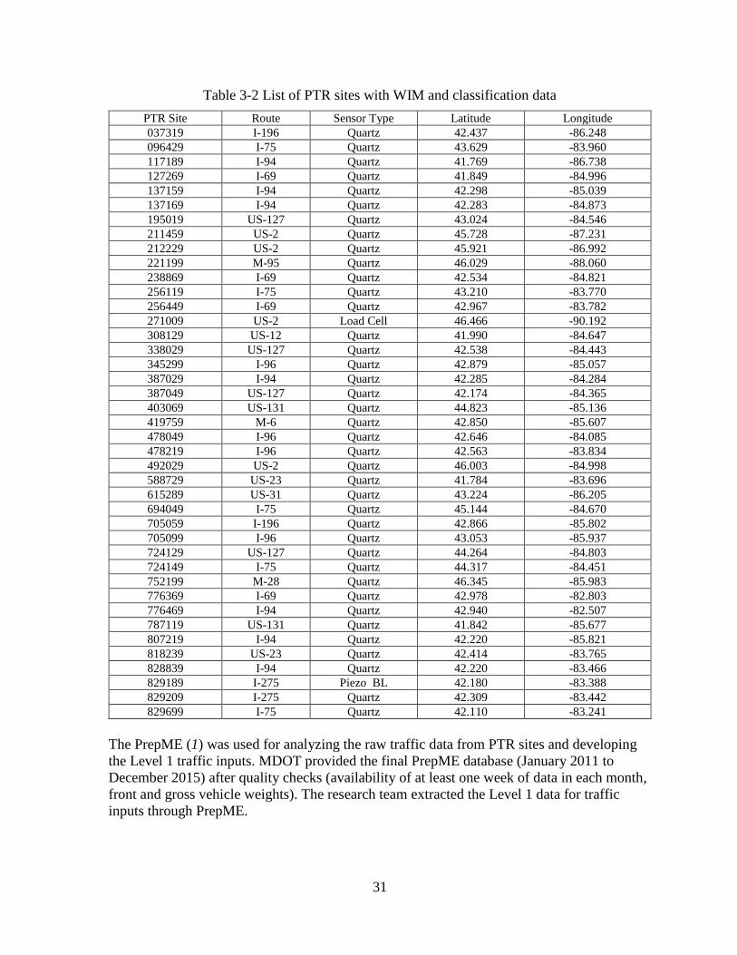
31
Table 3-2 List of PTR sites with WIM and classification data
PTR Site Route Sensor Type Latitude Longitude
037319 I-196 Quartz 42.437 -86.248
096429 I-75 Quartz 43.629 -83.960
117189 I-94 Quartz 41.769 -86.738
127269 I-69 Quartz 41.849 -84.996
137159 I-94 Quartz 42.298 -85.039
137169 I-94 Quartz 42.283 -84.873
195019 US-127 Quartz 43.024 -84.546
211459 US-2 Quartz 45.728 -87.231
212229 US-2 Quartz 45.921 -86.992
221199 M-95 Quartz 46.029 -88.060
238869 I-69 Quartz 42.534 -84.821
256119 I-75 Quartz 43.210 -83.770
256449 I-69 Quartz 42.967 -83.782
271009 US-2 Load Cell 46.466 -90.192
308129 US-12 Quartz 41.990 -84.647
338029 US-127 Quartz 42.538 -84.443
345299 I-96 Quartz 42.879 -85.057
387029 I-94 Quartz 42.285 -84.284
387049 US-127 Quartz 42.174 -84.365
403069 US-131 Quartz 44.823 -85.136
419759 M-6 Quartz 42.850 -85.607
478049 I-96 Quartz 42.646 -84.085
478219 I-96 Quartz 42.563 -83.834
492029 US-2 Quartz 46.003 -84.998
588729 US-23 Quartz 41.784 -83.696
615289 US-31 Quartz 43.224 -86.205
694049 I-75 Quartz 45.144 -84.670
705059 I-196 Quartz 42.866 -85.802
705099 I-96 Quartz 43.053 -85.937
724129 US-127 Quartz 44.264 -84.803
724149 I-75 Quartz 44.317 -84.451
752199 M-28 Quartz 46.345 -85.983
776369 I-69 Quartz 42.978 -82.803
776469 I-94 Quartz 42.940 -82.507
787119 US-131 Quartz 41.842 -85.677
807219 I-94 Quartz 42.220 -85.821
818239 US-23 Quartz 42.414 -83.765
828839 I-94 Quartz 42.220 -83.466
829189 I-275 Piezo BL 42.180 -83.388
829209 I-275 Quartz 42.309 -83.442
829699 I-75 Quartz 42.110 -83.241
The PrepME (1) was used for analyzing the raw traffic data from PTR sites and developing
the Level 1 traffic inputs. MDOT provided the final PrepME database (January 2011 to
December 2015) after quality checks (availability of at least one week of data in each month,
front and gross vehicle weights). The research team extracted the Level 1 data for traffic
inputs through PrepME.
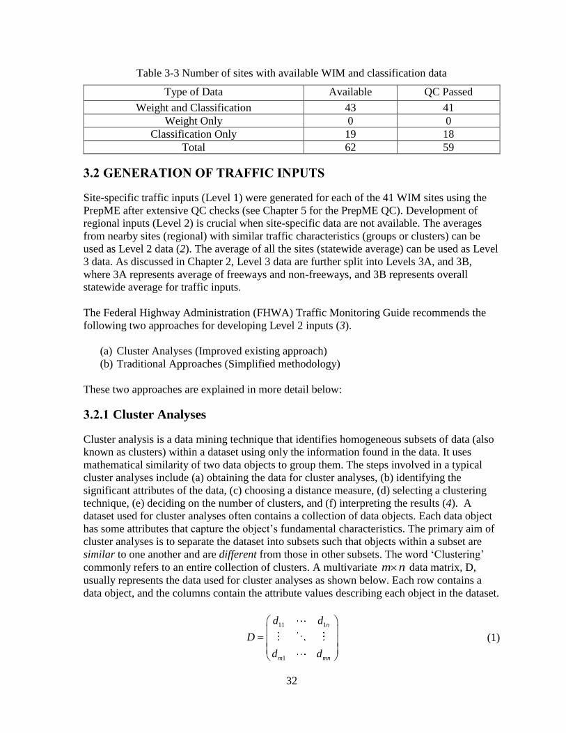
32
Table 3-3 Number of sites with available WIM and classification data
Type of Data Available QC Passed
Weight and Classification 43 41
Weight Only 0 0
Classification Only 19 18
Total 62 59
3.2 GENERATION OF TRAFFIC INPUTS
Site-specific traffic inputs (Level 1) were generated for each of the 41 WIM sites using the
PrepME after extensive QC checks (see Chapter 5 for the PrepME QC). Development of
regional inputs (Level 2) is crucial when site-specific data are not available. The averages
from nearby sites (regional) with similar traffic characteristics (groups or clusters) can be
used as Level 2 data (2). The average of all the sites (statewide average) can be used as Level
3 data. As discussed in Chapter 2, Level 3 data are further split into Levels 3A, and 3B,
where 3A represents average of freeways and non-freeways, and 3B represents overall
statewide average for traffic inputs.
The Federal Highway Administration (FHWA) Traffic Monitoring Guide recommends the
following two approaches for developing Level 2 inputs (3).
(a) Cluster Analyses (Improved existing approach)
(b) Traditional Approaches (Simplified methodology)
These two approaches are explained in more detail below:
3.2.1 Cluster Analyses
Cluster analysis is a data mining technique that identifies homogeneous subsets of data (also
known as clusters) within a dataset using only the information found in the data. It uses
mathematical similarity of two data objects to group them. The steps involved in a typical
cluster analyses include (a) obtaining the data for cluster analyses, (b) identifying the
significant attributes of the data, (c) choosing a distance measure, (d) selecting a clustering
technique, (e) deciding on the number of clusters, and (f) interpreting the results (4). A
dataset used for cluster analyses often contains a collection of data objects. Each data object
has some attributes that capture the object’s fundamental characteristics. The primary aim of
cluster analyses is to separate the dataset into subsets such that objects within a subset are
similar to one another and are different from those in other subsets. The word ‘Clustering’
commonly refers to an entire collection of clusters. A multivariate m n data matrix, D,
usually represents the data used for cluster analyses as shown below. Each row contains a
data object, and the columns contain the attribute values describing each object in the dataset.
11 1
1
n
m mn
d d
D
d d
(1)

33
where:
ijd = value of the jth attribute of object i.
Attributes of the data objects in the matrix may either be continuous, or ordinal or a mixture
of both. Some attributes of an object might not define it very well and might be irrelevant.
Such attributes should be excluded if possible, or weights could be added to the essential
attributes in the data matrix (4). Most clustering techniques convert the data matrix into a
m m ‘distance matrix’ of inter-object similarities or dissimilarities. The
similarity/dissimilarity between two objects with attributes on a continuous scale is a
numerical measure of the degree to which they are alike. Two objects are said to be close to
each other when the dissimilarity is small. Several similarity measures can express likeness
between a pair of objects. In general, two categories broadly define these measures: (a)
distance, and (b) correlation-type. ‘Euclidean Distance’ is the most commonly used distance
measure which is the straight line distance between two objects. It is calculated using
Equation (2).
1/2
2
,
1
( )
i j
p
o o ik jk
k
d o o (2)
where;
,ik jko o = kth component of the p-dimensional objects ,i jo o
To illustrate, consider six two dimensional points (or objects) with x and y coordinates as
follows (5): (a) P1 (0.40, 0.53), (b) P2 (0.22,0.38), (c) P3 (0.35,0.32), and (d) P4 (0.26,0.19),
(e) P5 (0.08, 0.41), and P6 (0.45, 0.30).The distance calculation between P1 and P2 is as
follows:
2 2(1,2) (0.40 0.22) (0.53 0.38) 0.234 dist (3)
Likewise, the distances between all possible pairs of objects can be computed and expressed
in the form of a ‘distance matrix.' The non-diagonal elements in this matrix represent the
distances between pairs of objects and the diagonal elements represent the distance from each
object to itself (hence, they are always zero) as seen in Equation (4) (6). The objects used in
this example has only two dimensions (attributes), but distances for objects with more than
two attributes can be computed (e.g., Monthly adjustment factors would have twelve
attributes, i.e., one for each month).

34
1 2 3 4 5 6
1
2
3
4
5
6
0 0.23 0.22 0.37 0.34 0.24
0.23 0 0.14 0.19 0.14 0.24
0.22 0.14 0 0.16 0.28 0.10
0.37 0.19 0.16 0 0.28 0.22
0.34 0.14 0.28 0.28 0 0.39
0.24 0.24 0.10 0.22 0.39 0
P P P P P P
P
P
dist matrix P
P
P
P
(4)
Mikowski distance is a more generalized form of the Euclidean distance as seen in Equation
(5). When r is equal to 1, it is called ‘Manhattan’ or ‘City block’ distance which is the
distance between two points measured at right angles along the axes.
1/
1
( , ) | |
rn
r
k k
k
d x y x y
(5)
The other commonly used similarity measure is the ‘Mahalanobis’ distance as shown in
Equation (6). It is a generalization of the Euclidean distance and could be used when the
attributes of the data objects are correlated or have different ranges of values.
1Mahalanobis( , ) ( ) ( )Tx y x y x y (6)
where:
= covariance matrix whose ijth entry is the covariance of the ith and jth attribute 1 = inverse of the covariance matrix
Correlation measures are the other category of similarity measures. The most widely used
correlation measure is the Pearson correlation coefficient (7). The correlation between two
data objects is a measure of the linear relationship between their attributes. A correlation
value of ‘1’ indicates a strong relationship, and a value of ‘-1’ indicates a fragile relationship
between the data objects and is calculated using Equation (7).
covariance( , )
( , )( ) ( )
xy
x y
x ycorr x y
stdev x stdev y
(7)
A number of similarity/dissimilarity measures exist, which makes choosing a measure for
cluster analyses a challenge. Earlier research studies have come up with categorizations of
the similarity or dissimilarity measures based on the critical properties of the data ( e.g., scale
of data, metric, and Euclidean properties of similarity matrices). However, the properties are
not very conclusive for choosing between the measures (7-11). The general observation is
that the nature of the data should strongly influence the choice of the similarity measure.
Sometimes, a similarity measure may already have been used previously and thus may have
answered the choice of the similarity measure. Occasionally, the clustering technique might
limit the choices of the similarity measures that could be used. Different similarity measures
can be used to see which ones produce more realistic results. However, for continuous data,

35
distance measures should be used when the magnitude of the data is essential. Assuming that
the attributes of a data object (e.g., the traffic volume in January does not affect the traffic
volume in February) are not correlated, the Euclidean distance was chosen as the similarity
measure in this study as it can be easily interpreted. More information on the choice of
similarity or dissimilarity measure and a decision-making table that may help choose the
similarity measure can be found in the literature (5, 10).
Clustering techniques divide data into a set of clusters commonly referred to as ‘clusterings.’
While the clusterings can be described in many ways, the commonly used distinction
between different types of clusterings is whether it is partitional or hierarchical. A partitional
clustering is merely a division of the set of data objects into nonoverlapping subsets (clusters)
such that each data object is precisely in one subset. If these clusters are permitted to have
sub-clusters, then a hierarchical clustering is obtained. The most commonly used clustering
techniques (5) are discussed below.
3.2.1.1 K-means
It is a partitional clustering technique that divides the dataset into a predetermined number of
clusters. The algorithm includes choosing ‘K’ initial centroids (which equals the desired
number of clusters). Each data object is assigned to the closest centroid, and each collection
of data objects assigned to a centroid forms a cluster. After each iteration, the centroid of
each cluster is updated based on the data objects assigned to that cluster. The iterations stop
when no objects change clusters, or equivalently, the centroids remain the same. Only a few
times, K-means reaches a state in which no objects are shifting from one cluster to another.
Usually, a rule is set to stop the iterations after reaching a steady state (e.g., only less than 1%
of the objects are changing the clusters) (5). Like every clustering technique, K-means needs
a similarity measure to assign the object to a centroid. As discussed before, several options
exist, but the most often used measure is the Euclidean distance. Given two sets of clusters
from different K-means runs, the overall sum of squared error (SSE) often decides the better
cluster as shown below (5).
2
1
( , )i
K
i
i x C
SSE dist c x
(8)
where:
K = number of clusters
iC = cluster iC
ic = centroid of cluster ic
x = data object in cluster iC
The mean of a cluster is always the best centroid for minimizing the SSE of a cluster and is
shown below. By minimizing the SSE of cluster K and solving for its centroid,

36
2
1
2
1
( )
( )
2 ( ) 0
12 ( ) 0
i
i
i
k k k
K
i
i x Ck k
K
i
i x C k
i
x C
K K K
k k k k k k k
x C x C x Ck
SSE c xc c
= c xc
= c x
c x m c x c x m
where:
km = number of objects in the cluster K
kx = data object in cluster kC
While K-means is a very general algorithm that can be used with different data types, it has
various limitations. One of them is choosing the initial centroids. Randomly choosing the
initial centroids often results in poor clusters and sometimes in empty clusters. While there
are remedies, it is often an exhaustive procedure to find the optimum initial centroids. One
procedure would be to run K-means multiple times with random initial centroids and use the
one with the least SEE. Another procedure is to use the hierarchical clustering at first to find
the clusters and their centroids and then rerun the K-means. Also, the number of clusters
required is an input into the K-means algorithm, which can be difficult to determine before
the clustering. For these reasons, K-means technique will not be used in the cluster analyses
of traffic data.
3.2.1.2 Hierarchical Clustering
Hierarchical clustering techniques are another prominent category of clustering methods.
There are two approaches for generating hierarchical clusterings (a) divisive, and (b)
agglomerative. In divisive clustering approach, all the objects in the dataset are considered as
a single cluster at the beginning and are divided it into two clusters at each stage until all the
clusters have only a single object. In the first step of the clustering, all the possible partitions
of the dataset need to be considered which equals to 12 1n combinations (where n is the
number of data objects). The large number of combinations makes divisive clustering
difficult to implement. Agglomerative approach performs clustering in an opposite manner as
compared to divisive approach. Agglomerative clustering technique considers each object in
the dataset as an individual cluster and merges them one at a time in a series of sequential
steps (12). The number of clusters during the first step equals the number of objects in the
dataset. At each subsequent step, the clusters that are ‘closest’ (or most similar) to each other
are merged to form a new cluster. The final step merges all the objects in the dataset into one
single cluster. The objects that are merged to form clusters at each step cannot be reassigned
to different clusters at a later stage. Agglomerative hierarchical clustering technique is
characterized by two choices: (a) the measurement of similarity between two objects in a
dataset, and (b) the type of linkage between clusters (5, 13). The clusters formed using the
hierarchical techniques can be represented using a two-dimensional diagram known as a
‘dendrogram.' A dendrogram illustrates the clusters formed at each stage of the clustering

37
process. Figure 3-1 shows an example of a dendrogram. Two clusters are merged at each step
of the process at a distance, or the height represented by the y-axis. The clustering technique
(or the ‘linkage type’) needs to be established after choosing the distance or similarity
measure (6). Discussed below are the most commonly used methods.
Figure 3-1 An example of the dendrogram
Single Linkage Method
This method is also called the nearest neighbor or minimum method. The similarity between
two clusters is the minimum of the distance between any two objects in two different clusters
(12). Consider the six two dimensional points and the distance matrix discussed above [see
Equation (4)]. In the first step of this clustering technique, points ‘3’ and ‘6’ are merged into
a cluster (see Figure 3-2a) because they have the smallest distance of 0.102 between them.
*5*2
*6*3II
III
I
*4
*1
IV
V
(a)
(b)
Figure 3-2 Single linkage clustering

38
As seen in Figure 3-2b (dendrogram), that is the height at which they are merged into a single
cluster. In the second step, points ‘2’ and ‘5’ are merged into a cluster. The distances
between the newly formed clusters in step 3 are calculated as follows:
({3,6},{2,5}) min( (3,2), (6,2), (3,5), (6,5))
min(0.143,0.244,0.285,0.386) 0.143
({3,6},{4}) min( (3,4), (6,4), )
dist dist dist dist dist
dist dist dist
min(0.158,0.220) 0.158
In the third step, the clusters {3,6},{2,5} are combined to form a third cluster at the height of
0.143 as seen in the dendrogram. This process goes on until all the points are combined into
one single cluster at the height of approximately 0.22.
Complete Linkage Method
This method is also called the furthest neighbor or maximum method. The similarity of two
clusters is defined as the maximum of the distance between any two points in two clusters.
As with the single linkage method, clusters{3,6}and{2,5} are formed first (See Figure 3-3a
and 3-3b).
*5*2
*6*3
II
IV
I*4
*1
III
V
(a)
(b)
Figure 3-3 Complete linkage clustering
In the third step, instead of{3,6}and{2,5}merging next, {3,6} is merged with {4}because the
procedure takes into account the least maximum distance between clusters.

39
({3,6},{2,5}) max( (3,2), (6,2), (3,5), (6,5))
max(0.143,0.244,0.285,0.386) 0.386
({3,6},{4}) max( (3,4), (6,4))
dist dist dist dist dist
dist dist dist
max(0.158,0.220) 0.220
({3,6},{1}) max( (3,1), (6,1))
max(0.216,0.235) 0.235
dist dist dist
Group Average Method
For the group average version of hierarchical clustering, the similarity of two clusters is the
average of pairwise similarity among all pairs of points in the different clusters. Group
average method is an intermediate approach to the single, and complete link approaches.
Figure 3-4 shows the dendrogram for this method.
The similarity between two clusters A and B of sizes An and Bn is calculated using Equation
(9).
( , )
( , )*
a A b B
A B
dist a b
proximity A Bn n
(9)
*5
*2
*6*3
II
IV
I*4
*1
III
V
(a)
(b)
Figure 3-4 Group average clustering
An illustration of group average method is given below.

40
(3,1) (6,1), (4,1)({3,6,4},{1}) 0.273
(3 1)
(2,1) (5,1)({2,5},{1}) 0.288
(2 1)
(3,2) (3,5) (6,2) (6,5) (4,2) (4,5)({3,6,4},{2,5})
(
dist dist distdist
dist distdist
dist dist dist dist dist distdist
0.256
3 2)
Because ({3,6,4},{2,5})dist is smaller than ({3,6,4},{1})dist and ({2,5},{1})dist , clusters
{3,6,4} and {2,5}are merged in the fourth step.
Ward’s Method
Ward’s method is another general agglomerative hierarchical clustering technique. The
similarity of two clusters depends on an objective functions’ optimal value. The most widely
used objective function is the error sum of squares or within-cluster variance. Clusters with
the least increase in the overall within-cluster variance when combined are merged at each
step. Figures 3-5a and 3-5b show the dendrogram for this method.
*5*2
*6*3
II
IV
I
*4
*1
III
V
(a)
(b)
Figure 3-5 Ward’s method of clustering
The similarity between two clusters A and B of sizes An and Bn can be calculated by using
Equation (10), where AC and BC are the centroids of clusters A and B.
2
( , ) ( , )A BA B
A B
n nproximity A B dist C C
n n
(10)

41
In the first two steps, {3,6} and {2,5} are combined separately because of the least increase
in the sum of squares when combined. The third step is illustrated below.
2 2 1({3,6},{4}) ({3,6},{4}) 0.213
(2 1)
2 2 1({3,6},{1}) ({3,6},{1}) 0.254
(2 1)
2 2 2({3,6},{2,5}) ({3,6},{2,5}) 0.373
(2 2)
dist dist
dist dist
dist dist
The third step combines clusters {3,6}and{4}since the increase in the sum of squares is
minimum among other combinations.
The different linkage methods discussed above define the distance between the pair of
clusters in a certain way. Each of these linkage algorithms can yield entirely different results
when used on the same dataset. The single linkage method tends to produce one large cluster
with other clusters containing very few objects because several clusters may be joined
together (called ‘chaining effect’) merely because one of their objects is within proximity of
an object from a separate cluster. This problem is specific to single linkage because only the
minimum distance between objects is used. As mentioned before, the objects that are merged
to form clusters at one step cannot be reassigned to different clusters at a later stage, and
therefore the chaining effect could lead to abnormal clusters. However, single linkage
method can be used to detect the outliers, as these will always be merged during the final step
of the clustering process (6, 12). Complete linkage method solves the problem of chaining.
However, they tend to produce large globular clusters. Outliers can profoundly influence the
outcome of the clusters as this clustering technique uses the maximum distance between the
objects. The average link method is a compromise between the single and complete linkage
methods as it takes into account the average distances between the objects. This method is
relatively robust compared to the single and complete linkage methods as it takes into
account the cluster structure (7). Ward’s method is sensitive to outliers and tends to find
same size and spherical clusters. The average linkage and Ward's method are the most
frequently used methods. There are no guidelines on choosing the right linkage method.
However, some studies found that Ward’s method performed better than the average linkage
method (14). Therefore, Ward’s method was used for cluster analyses of the traffic data.
The advantages of cluster analyses are that the groups are formed objectively (based on a
mathematical function) and not subjected to bias or subjective decisions. The other advantage
is that it finds patterns in the data that are not intuitively obvious therefore providing new
insights into traffic patterns in a region. One main disadvantage is the lack of guidelines on
establishing the optimal number of clusters. While various techniques were developed to
identify the optimal number of clusters, none of them are perfect and have their drawbacks.
The other disadvantage is that, since clustering is purely a mathematical technique, the
objects in a cluster might not have the same identifiable attributes making the assignment of
data from a new location to the existing clusters difficult. However, the advantages outweigh
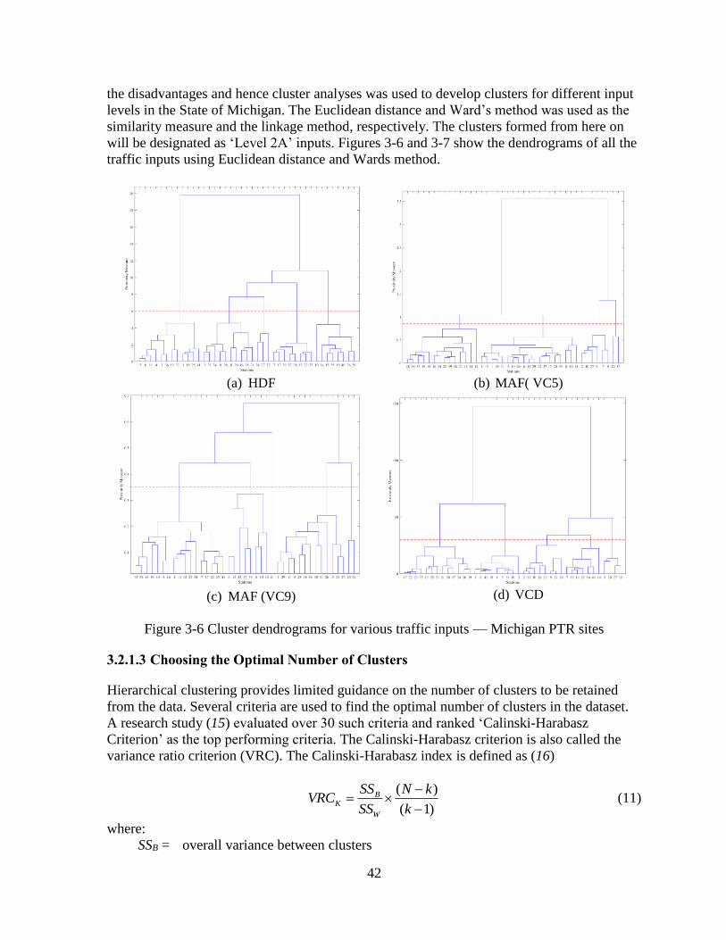
42
the disadvantages and hence cluster analyses was used to develop clusters for different input
levels in the State of Michigan. The Euclidean distance and Ward’s method was used as the
similarity measure and the linkage method, respectively. The clusters formed from here on
will be designated as ‘Level 2A’ inputs. Figures 3-6 and 3-7 show the dendrograms of all the
traffic inputs using Euclidean distance and Wards method.
(a) HDF
(b) MAF( VC5)
(c) MAF (VC9)
(d) VCD
Figure 3-6 Cluster dendrograms for various traffic inputs — Michigan PTR sites
3.2.1.3 Choosing the Optimal Number of Clusters
Hierarchical clustering provides limited guidance on the number of clusters to be retained
from the data. Several criteria are used to find the optimal number of clusters in the dataset.
A research study (15) evaluated over 30 such criteria and ranked ‘Calinski-Harabasz
Criterion’ as the top performing criteria. The Calinski-Harabasz criterion is also called the
variance ratio criterion (VRC). The Calinski-Harabasz index is defined as (16)
( )
( 1)
BK
W
SS N kVRC
SS k (11)
where:
SSB = overall variance between clusters
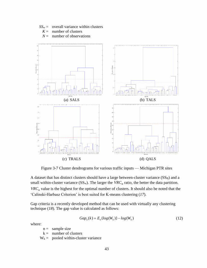
43
SSw = overall variance within clusters
K = number of clusters
N = number of observations
(a) SALS
(b) TALS
(c) TRALS
(d) QALS
Figure 3-7 Cluster dendrograms for various traffic inputs — Michigan PTR sites
A dataset that has distinct clusters should have a large between-cluster variance (SSB) and a
small within-cluster variance (SSw). The larger the KVRC ratio, the better the data partition.
KVRC value is the highest for the optimal number of clusters. It should also be noted that the
‘Calinski-Harbasz Criterion’ is best suited for K-means clustering (17).
Gap criteria is a recently developed method that can be used with virtually any clustering
technique (18). The gap value is calculated as follows:
( ) { ( )} ( )n n k kE log W loGap gk W (12)
where:
n = sample size
k = number of clusters
Wk = pooled within-cluster variance
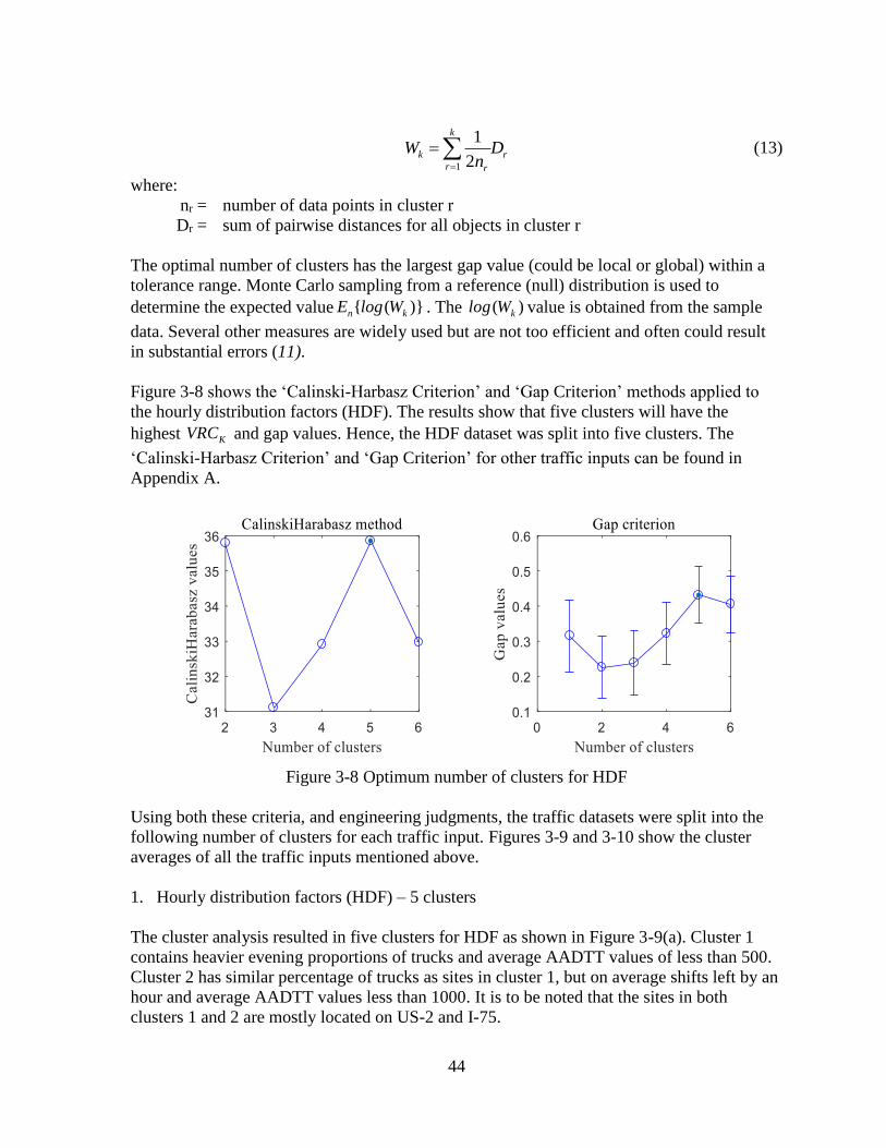
44
1
1
2
k
k r
r r
W Dn
(13)
where:
nr = number of data points in cluster r
Dr = sum of pairwise distances for all objects in cluster r
The optimal number of clusters has the largest gap value (could be local or global) within a
tolerance range. Monte Carlo sampling from a reference (null) distribution is used to
determine the expected value { ( )}n kE log W . The ( )klog W value is obtained from the sample
data. Several other measures are widely used but are not too efficient and often could result
in substantial errors (11).
Figure 3-8 shows the ‘Calinski-Harbasz Criterion’ and ‘Gap Criterion’ methods applied to
the hourly distribution factors (HDF). The results show that five clusters will have the
highest KVRC and gap values. Hence, the HDF dataset was split into five clusters. The
‘Calinski-Harbasz Criterion’ and ‘Gap Criterion’ for other traffic inputs can be found in
Appendix A.
Figure 3-8 Optimum number of clusters for HDF
Using both these criteria, and engineering judgments, the traffic datasets were split into the
following number of clusters for each traffic input. Figures 3-9 and 3-10 show the cluster
averages of all the traffic inputs mentioned above.
1. Hourly distribution factors (HDF) – 5 clusters
The cluster analysis resulted in five clusters for HDF as shown in Figure 3-9(a). Cluster 1
contains heavier evening proportions of trucks and average AADTT values of less than 500.
Cluster 2 has similar percentage of trucks as sites in cluster 1, but on average shifts left by an
hour and average AADTT values less than 1000. It is to be noted that the sites in both
clusters 1 and 2 are mostly located on US-2 and I-75.
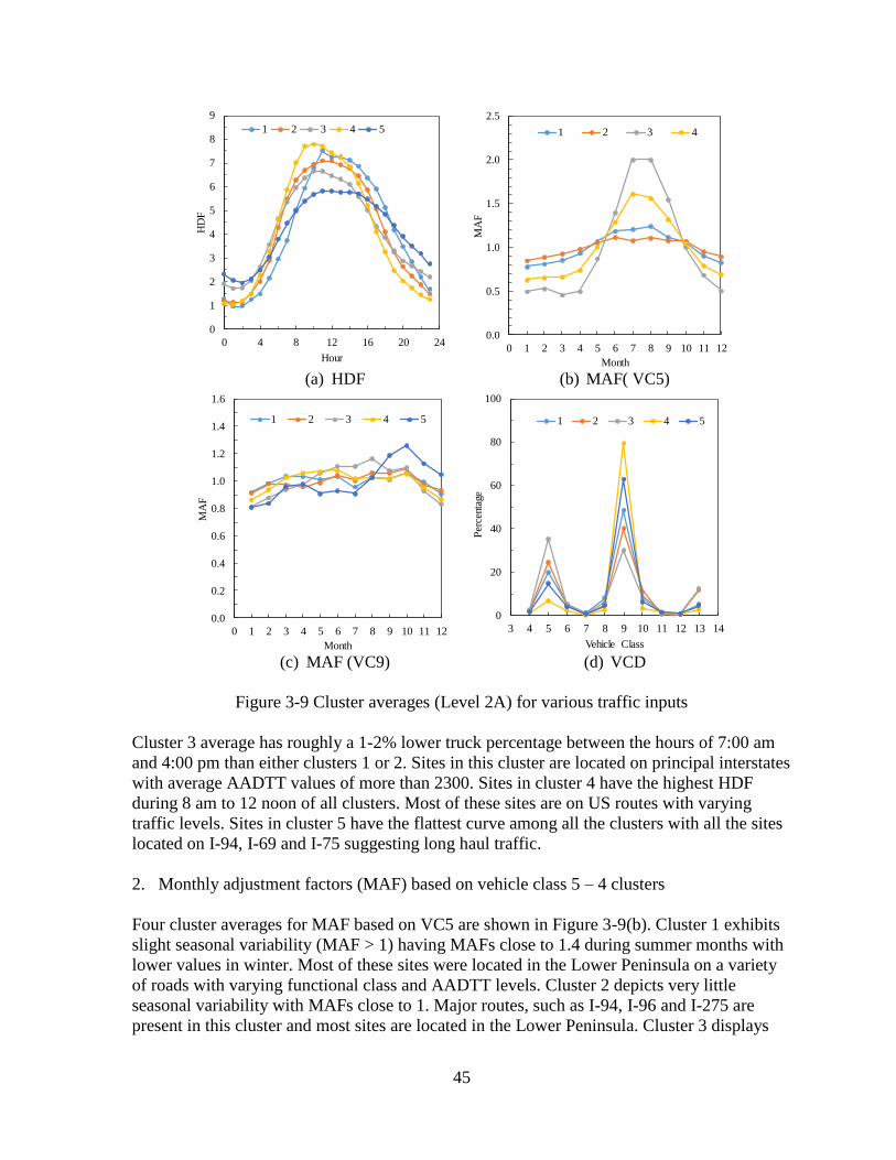
45
(a) HDF
(b) MAF( VC5)
(c) MAF (VC9)
(d) VCD
Figure 3-9 Cluster averages (Level 2A) for various traffic inputs
Cluster 3 average has roughly a 1-2% lower truck percentage between the hours of 7:00 am
and 4:00 pm than either clusters 1 or 2. Sites in this cluster are located on principal interstates
with average AADTT values of more than 2300. Sites in cluster 4 have the highest HDF
during 8 am to 12 noon of all clusters. Most of these sites are on US routes with varying
traffic levels. Sites in cluster 5 have the flattest curve among all the clusters with all the sites
located on I-94, I-69 and I-75 suggesting long haul traffic.
2. Monthly adjustment factors (MAF) based on vehicle class 5 – 4 clusters
Four cluster averages for MAF based on VC5 are shown in Figure 3-9(b). Cluster 1 exhibits
slight seasonal variability (MAF > 1) having MAFs close to 1.4 during summer months with
lower values in winter. Most of these sites were located in the Lower Peninsula on a variety
of roads with varying functional class and AADTT levels. Cluster 2 depicts very little
seasonal variability with MAFs close to 1. Major routes, such as I-94, I-96 and I-275 are
present in this cluster and most sites are located in the Lower Peninsula. Cluster 3 displays
0
1
2
3
4
5
6
7
8
9
0 4 8 12 16 20 24
HD
F
Hour
1 2 3 4 5
0.0
0.5
1.0
1.5
2.0
2.5
0 1 2 3 4 5 6 7 8 9 10 11 12
MA
F
Month
1 2 3 4
0.0
0.2
0.4
0.6
0.8
1.0
1.2
1.4
1.6
0 1 2 3 4 5 6 7 8 9 10 11 12
MA
F
Month
1 2 3 4 5
0
20
40
60
80
100
3 4 5 6 7 8 9 10 11 12 13 14
Per
cent
age
Vehicle Class
1 2 3 4 5

46
higher MAF in summer and fall, with much lower MAF in winter and spring. However there
are only two sites (M-28 and US-2) in this cluster and are located in the Upper Peninsula
with low AADTT. Sites in cluster 4 also have higher MAF in summer and fall and are
mostly located on north-south routes such as I-75 and US-127.
3. MAF based on vehicle class 9 – 5 clusters
Five cluster averages for MAF based on VC9 are shown in Figure 3-9(c). Almost all the sites
in all the clusters have no seasonal variability between months. Since, VC9 trucks are used
for long haul throughout the year, a uniform presence of such trucks is expected on all the
sites.
4. Vehicle class distribution (VCD) – 5 clusters
Figure 3-9 (d) illustrates the five clusters, each distinguished by the percentage of VC5 and
VC9. While four clusters have higher VC9 truck levels than VC5, their proportions are
different. Sites in cluster 1 have percentage VC9 trucks in the ranges of 45 to 70 while the
VC5 truck percentage was in the range of 15 to 25. Most of these sites were found on state
routes such as US-127 and US-2 with one-way AADTT ranging from 700 to 3600. Cluster 2
contained a majority of sites with percentage VC9 trucks less than 45 while the VC5 truck
percentage was in the range of 20 to 30. Sites in this cluster are located mostly on rural
arterials, such as US-2, US-31, M-95, generally with AADTT of less than 1500. Cluster 3 has
sites that have slightly higher percentage of VC5 trucks than VC9 trucks. Most of these sites
are on rural arterials with an AADTT of less than 800. Sites in cluster 4 have the highest
percentage of VC9 trucks (above 75) with very low percentage of VC5 trucks (below 10). All
the sites in this cluster are located on I-94, I-69 and I-75 with AADTT values ranging from
2500 to 8000. Sites in cluster 5 have percentage of VC9 trucks between 55 and 70 with
percentage of VC5 trucks between 10 and 20. Most of the sites in this cluster are located on
the interstates with a few sites on US-23. The AADTT values ranging from 1200 to 3500.
5. Single axle load spectra (SALS) based on vehicle class 5 – 4 clusters
Single axle load spectra are generally represented by VC5. Therefore, the single axle load
spectra data for VC5 trucks were clustered and the cluster averages are shown Figure 3-10
(a). Four clusters were formed and are directly related to the peaks observed in the data. For
all the sites in the clusters the first peak occurs at approximately 4 to 6 kips while the second
peak occurs at 8 to 10 kips. A review of the individual single axles for all VCs at all sites
revealed that the axle load spectra is not influenced so much by the shape of the axle load
spectra itself but instead the actual distribution of the truck traffic, particularly the presence
of VC5. Cluster 1 has almost equal proportion of axles in the 4-6 kip range and the 8-10 kip
range. Cluster 2 has higher proportion of 4-6 kip axles than 8-10 kip axles. The sites located
in clusters 1 and 2 are a mixture of interstates and state routes and have varying AADTT
levels. Cluster 3 has only one site (US-2) in the Upper Peninsula and the pattern seen in the
figure is unique to that site. Cluster 4 has sites with higher proportion of axles in the 8-10 kip
range than the 4-6 kip range. All the sites in this cluster are located on I-94, I-96 and I-75
with AADTT levels ranging from 1500 to 8300.
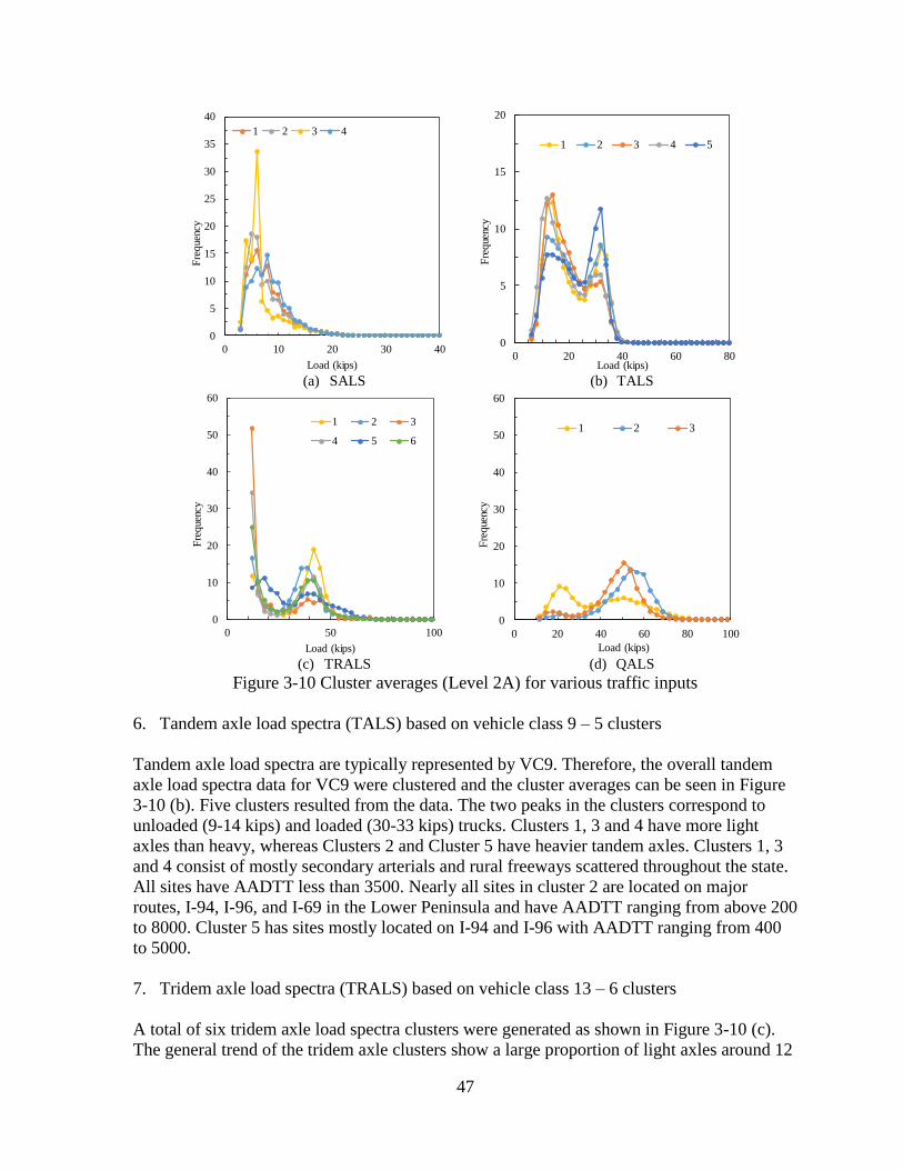
47
(a) SALS
(b) TALS
(c) TRALS
(d) QALS
Figure 3-10 Cluster averages (Level 2A) for various traffic inputs
6. Tandem axle load spectra (TALS) based on vehicle class 9 – 5 clusters
Tandem axle load spectra are typically represented by VC9. Therefore, the overall tandem
axle load spectra data for VC9 were clustered and the cluster averages can be seen in Figure
3-10 (b). Five clusters resulted from the data. The two peaks in the clusters correspond to
unloaded (9-14 kips) and loaded (30-33 kips) trucks. Clusters 1, 3 and 4 have more light
axles than heavy, whereas Clusters 2 and Cluster 5 have heavier tandem axles. Clusters 1, 3
and 4 consist of mostly secondary arterials and rural freeways scattered throughout the state.
All sites have AADTT less than 3500. Nearly all sites in cluster 2 are located on major
routes, I-94, I-96, and I-69 in the Lower Peninsula and have AADTT ranging from above 200
to 8000. Cluster 5 has sites mostly located on I-94 and I-96 with AADTT ranging from 400
to 5000.
7. Tridem axle load spectra (TRALS) based on vehicle class 13 – 6 clusters
A total of six tridem axle load spectra clusters were generated as shown in Figure 3-10 (c).
The general trend of the tridem axle clusters show a large proportion of light axles around 12
0
5
10
15
20
25
30
35
40
0 10 20 30 40
Fre
que
ncy
Load (kips)
1 2 3 4
0
5
10
15
20
0 20 40 60 80
Fre
que
ncy
Load (kips)
1 2 3 4 5
0
10
20
30
40
50
60
0 50 100
Fre
que
ncy
Load (kips)
1 2 3
4 5 6
0
10
20
30
40
50
60
0 20 40 60 80 100
Fre
que
ncy
Load (kips)
1 2 3
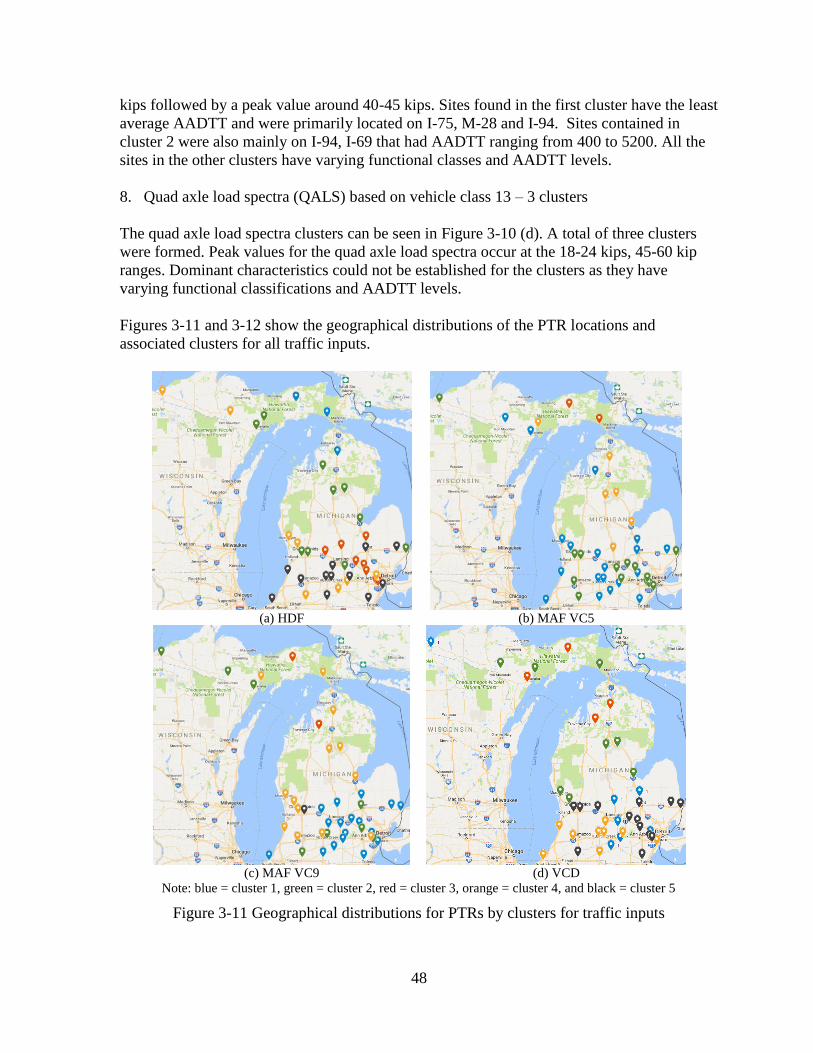
48
kips followed by a peak value around 40-45 kips. Sites found in the first cluster have the least
average AADTT and were primarily located on I-75, M-28 and I-94. Sites contained in
cluster 2 were also mainly on I-94, I-69 that had AADTT ranging from 400 to 5200. All the
sites in the other clusters have varying functional classes and AADTT levels.
8. Quad axle load spectra (QALS) based on vehicle class 13 – 3 clusters
The quad axle load spectra clusters can be seen in Figure 3-10 (d). A total of three clusters
were formed. Peak values for the quad axle load spectra occur at the 18-24 kips, 45-60 kip
ranges. Dominant characteristics could not be established for the clusters as they have
varying functional classifications and AADTT levels.
Figures 3-11 and 3-12 show the geographical distributions of the PTR locations and
associated clusters for all traffic inputs.
(a) HDF
(b) MAF VC5
(c) MAF VC9
(d) VCD
Note: blue = cluster 1, green = cluster 2, red = cluster 3, orange = cluster 4, and black = cluster 5
Figure 3-11 Geographical distributions for PTRs by clusters for traffic inputs
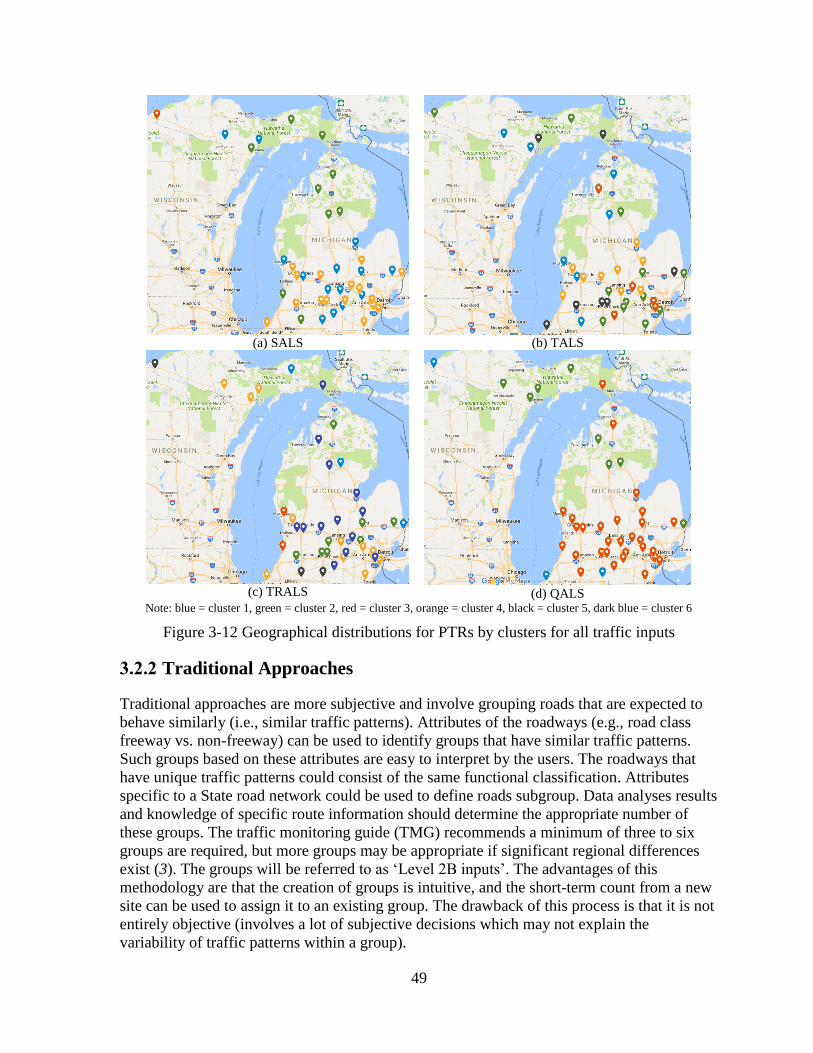
49
(a) SALS
(b) TALS
(c) TRALS
(d) QALS
Note: blue = cluster 1, green = cluster 2, red = cluster 3, orange = cluster 4, black = cluster 5, dark blue = cluster 6
Figure 3-12 Geographical distributions for PTRs by clusters for all traffic inputs
3.2.2 Traditional Approaches
Traditional approaches are more subjective and involve grouping roads that are expected to
behave similarly (i.e., similar traffic patterns). Attributes of the roadways (e.g., road class
freeway vs. non-freeway) can be used to identify groups that have similar traffic patterns.
Such groups based on these attributes are easy to interpret by the users. The roadways that
have unique traffic patterns could consist of the same functional classification. Attributes
specific to a State road network could be used to define roads subgroup. Data analyses results
and knowledge of specific route information should determine the appropriate number of
these groups. The traffic monitoring guide (TMG) recommends a minimum of three to six
groups are required, but more groups may be appropriate if significant regional differences
exist (3). The groups will be referred to as ‘Level 2B inputs’. The advantages of this
methodology are that the creation of groups is intuitive, and the short-term count from a new
site can be used to assign it to an existing group. The drawback of this process is that it is not
entirely objective (involves a lot of subjective decisions which may not explain the
variability of traffic patterns within a group).

50
The attributes used to classify groups need not necessarily be the same for all the traffic
inputs and instead should depend on the type of traffic input. For monthly adjustment and
hourly distribution factors, the primary groups could be based on road class and development
type such as (a) rural interstates, (b) rural non-interstates, (c) urban interstates, and (d) urban
non-interstates. The TMG recommends adding a fifth group which consists of roadways used
by recreational traffic (3). Recreational traffic patterns should be identified using local
knowledge of specific locations that could generate recreational traffic; they cannot be
defined based on functional class or area boundaries. An SHA could further expand these
four groups, but more groups may require more data (more WIM and classification sites)
which in turn would increase the cost to the agency. The coefficient of variation of monthly
patterns in urban areas is usually under 10 percent, while in rural areas it ranges between 10
and 25 percent. Values higher than 25 percent indicate highly variable travel patterns, which
reflect recreational patterns but may also be due to reasons other than recreational travel. For
MAF and HDF, functional class (freeway or non-freeway), development type (rural or
urban), and geographic location within the State have been the typical characteristics for
grouping the roadways. Recreational (or geographic) designations can be used for roads that
are affected by sizeable recreational traffic generators occasionally (3).
For VCD, characteristics of roadways to be considered for groupings should be different.
Previous research has found out that functional class of roadways have an inconsistent
relationship to truck travel patterns (19, 20). The amount of long-distance truck traffic versus
the amount of locally oriented truck traffic significantly affect the truck traffic patterns on a
route. Also the existence of significant truck traffic generators along a roadway such as
agriculture or significant industrial activity can affect these patterns. Functional road
classification helps in a limited way to differentiate between roads with heavy through-traffic
and those with only local traffic. Typically, interstates and principal arterials have higher
through-truck traffic volumes. However, there are roads with several lower functional
classifications that are carrying more through-truck volumes than the interstates and principal
arterials. Developing these groups also requires an understanding of the freight movements in
the State (19, 20). Communication with the staff at the SHA would help in identifying the
local and statewide patterns. Cluster analyses could be used to identify the traffic patterns
initially, and each cluster could be looked at to gain a fundamental idea of the roadway
characteristics of the PTR locations in that cluster.
Based on above discussion, for Level 2B inputs, the challenge lies in identifying a
combination of attributes that can be used to group the PTR locations. The traffic patterns at
the PTR locations should be similar within a group and should be different between the
groups. An automated process was developed to help identify such combinations of
attributes. The following attributes from the MDOT’s sufficiency database were identified
for grouping different PTR locations:
Functional classification (Freeway vs. Non-Freeway)
Development type (Urban vs. Rural)
One-way AADTT levels (1 “<1000”, 2 “1000-3000”,3 “>3000”)
Corridors of highest significance, COHS (National, Regional, and Statewide)

51
Number of lanes (2, 3 and 4)
Road type (Non-freeway divided, Non-freeway undivided, and Freeway)
Vehicle class 9 (VC 9) distribution levels (< 45, 45 – 70, >70)
It should be noted that the MDOT sufficiency database itself is no longer being supported,
but its data is still available in other platforms and is being updated. Several attributes can be
chosen at a time to divide the PTR locations into groups. Tables 3-4, to 3-6 list the possible
2-, 3-, and 4-way combinations of the attributes listed above. Each attribute has sublevels
(e.g., functional classification has two sublevels of freeway and non-freeway), and hence a
combination of attributes has different sublevel combinations. The Level 1 traffic inputs of
PTR sites belonging to a combination of sublevels are averaged. For example, the VCD
traffic inputs for the combination of functional class and development type (2-way
combination) can be seen in Table 3-7.
Table 3-4 Possible combination of attributes when chosen two at a time
Attribute 1 Attribute 2
Functional Class Road Type
Functional Class Number of Lanes
Functional Class Commercial AADT
Functional Class COHS
Functional Class Development Type
Functional Class VCD Level
Road Type Number of Lanes
Road Type Commercial AADT
Road Type COHS
Road Type Development Type
Road Type VCD Level
Number of Lanes Commercial AADT
Number of Lanes COHS
Number of Lanes Development Type
Number of Lanes VCD Level
Commercial AADT COHS
Commercial AADT Development Type
Commercial AADT VCD Level
COHS Development Type
COHS VCD Level
Development Type VCD Level
Note: There are 21 2-way attribute combinations (based on 7C2=21).
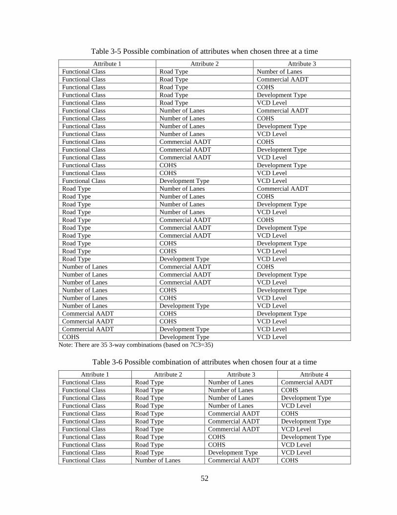
52
Table 3-5 Possible combination of attributes when chosen three at a time
Attribute 1 Attribute 2 Attribute 3
Functional Class Road Type Number of Lanes
Functional Class Road Type Commercial AADT
Functional Class Road Type COHS
Functional Class Road Type Development Type
Functional Class Road Type VCD Level
Functional Class Number of Lanes Commercial AADT
Functional Class Number of Lanes COHS
Functional Class Number of Lanes Development Type
Functional Class Number of Lanes VCD Level
Functional Class Commercial AADT COHS
Functional Class Commercial AADT Development Type
Functional Class Commercial AADT VCD Level
Functional Class COHS Development Type
Functional Class COHS VCD Level
Functional Class Development Type VCD Level
Road Type Number of Lanes Commercial AADT
Road Type Number of Lanes COHS
Road Type Number of Lanes Development Type
Road Type Number of Lanes VCD Level
Road Type Commercial AADT COHS
Road Type Commercial AADT Development Type
Road Type Commercial AADT VCD Level
Road Type COHS Development Type
Road Type COHS VCD Level
Road Type Development Type VCD Level
Number of Lanes Commercial AADT COHS
Number of Lanes Commercial AADT Development Type
Number of Lanes Commercial AADT VCD Level
Number of Lanes COHS Development Type
Number of Lanes COHS VCD Level
Number of Lanes Development Type VCD Level
Commercial AADT COHS Development Type
Commercial AADT COHS VCD Level
Commercial AADT Development Type VCD Level
COHS Development Type VCD Level
Note: There are 35 3-way combinations (based on 7C3=35)
Table 3-6 Possible combination of attributes when chosen four at a time
Attribute 1 Attribute 2 Attribute 3 Attribute 4
Functional Class Road Type Number of Lanes Commercial AADT
Functional Class Road Type Number of Lanes COHS
Functional Class Road Type Number of Lanes Development Type
Functional Class Road Type Number of Lanes VCD Level
Functional Class Road Type Commercial AADT COHS
Functional Class Road Type Commercial AADT Development Type
Functional Class Road Type Commercial AADT VCD Level
Functional Class Road Type COHS Development Type
Functional Class Road Type COHS VCD Level
Functional Class Road Type Development Type VCD Level
Functional Class Number of Lanes Commercial AADT COHS
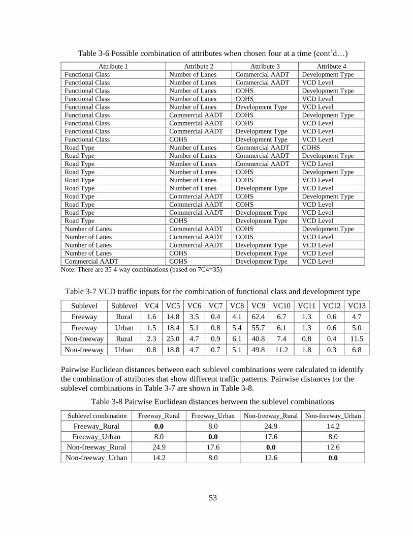
53
Table 3-6 Possible combination of attributes when chosen four at a time (cont’d…)
Attribute 1 Attribute 2 Attribute 3 Attribute 4
Functional Class Number of Lanes Commercial AADT Development Type
Functional Class Number of Lanes Commercial AADT VCD Level
Functional Class Number of Lanes COHS Development Type
Functional Class Number of Lanes COHS VCD Level
Functional Class Number of Lanes Development Type VCD Level
Functional Class Commercial AADT COHS Development Type
Functional Class Commercial AADT COHS VCD Level
Functional Class Commercial AADT Development Type VCD Level
Functional Class COHS Development Type VCD Level
Road Type Number of Lanes Commercial AADT COHS
Road Type Number of Lanes Commercial AADT Development Type
Road Type Number of Lanes Commercial AADT VCD Level
Road Type Number of Lanes COHS Development Type
Road Type Number of Lanes COHS VCD Level
Road Type Number of Lanes Development Type VCD Level
Road Type Commercial AADT COHS Development Type
Road Type Commercial AADT COHS VCD Level
Road Type Commercial AADT Development Type VCD Level
Road Type COHS Development Type VCD Level
Number of Lanes Commercial AADT COHS Development Type
Number of Lanes Commercial AADT COHS VCD Level
Number of Lanes Commercial AADT Development Type VCD Level
Number of Lanes COHS Development Type VCD Level
Commercial AADT COHS Development Type VCD Level
Note: There are 35 4-way combinations (based on 7C4=35)
Table 3-7 VCD traffic inputs for the combination of functional class and development type
Sublevel Sublevel VC4 VC5 VC6 VC7 VC8 VC9 VC10 VC11 VC12 VC13
Freeway Rural 1.6 14.8 3.5 0.4 4.1 62.4 6.7 1.3 0.6 4.7
Freeway Urban 1.5 18.4 5.1 0.8 5.4 55.7 6.1 1.3 0.6 5.0
Non-freeway Rural 2.3 25.0 4.7 0.9 6.1 40.8 7.4 0.8 0.4 11.5
Non-freeway Urban 0.8 18.8 4.7 0.7 5.1 49.8 11.2 1.8 0.3 6.8
Pairwise Euclidean distances between each sublevel combinations were calculated to identify
the combination of attributes that show different traffic patterns. Pairwise distances for the
sublevel combinations in Table 3-7 are shown in Table 3-8.
Table 3-8 Pairwise Euclidean distances between the sublevel combinations
Sublevel combination Freeway_Rural Freeway_Urban Non-freeway_Rural Non-freeway_Urban
Freeway_Rural 0.0 8.0 24.9 14.2
Freeway_Urban 8.0 0.0 17.6 8.0
Non-freeway_Rural 24.9 17.6 0.0 12.6
Non-freeway_Urban 14.2 8.0 12.6 0.0
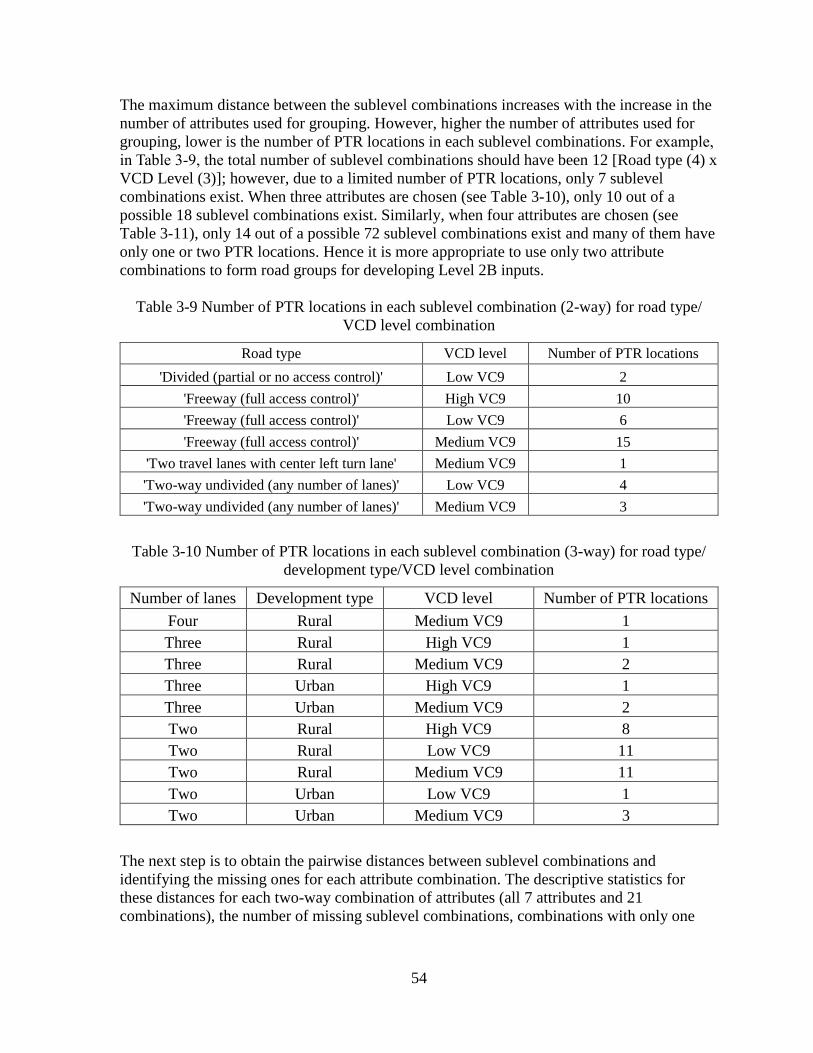
54
The maximum distance between the sublevel combinations increases with the increase in the
number of attributes used for grouping. However, higher the number of attributes used for
grouping, lower is the number of PTR locations in each sublevel combinations. For example,
in Table 3-9, the total number of sublevel combinations should have been 12 [Road type (4) x
VCD Level (3)]; however, due to a limited number of PTR locations, only 7 sublevel
combinations exist. When three attributes are chosen (see Table 3-10), only 10 out of a
possible 18 sublevel combinations exist. Similarly, when four attributes are chosen (see
Table 3-11), only 14 out of a possible 72 sublevel combinations exist and many of them have
only one or two PTR locations. Hence it is more appropriate to use only two attribute
combinations to form road groups for developing Level 2B inputs.
Table 3-9 Number of PTR locations in each sublevel combination (2-way) for road type/
VCD level combination
Road type VCD level Number of PTR locations
'Divided (partial or no access control)' Low VC9 2
'Freeway (full access control)' High VC9 10
'Freeway (full access control)' Low VC9 6
'Freeway (full access control)' Medium VC9 15
'Two travel lanes with center left turn lane' Medium VC9 1
'Two-way undivided (any number of lanes)' Low VC9 4
'Two-way undivided (any number of lanes)' Medium VC9 3
Table 3-10 Number of PTR locations in each sublevel combination (3-way) for road type/
development type/VCD level combination
Number of lanes Development type VCD level Number of PTR locations
Four Rural Medium VC9 1
Three Rural High VC9 1
Three Rural Medium VC9 2
Three Urban High VC9 1
Three Urban Medium VC9 2
Two Rural High VC9 8
Two Rural Low VC9 11
Two Rural Medium VC9 11
Two Urban Low VC9 1
Two Urban Medium VC9 3
The next step is to obtain the pairwise distances between sublevel combinations and
identifying the missing ones for each attribute combination. The descriptive statistics for
these distances for each two-way combination of attributes (all 7 attributes and 21
combinations), the number of missing sublevel combinations, combinations with only one
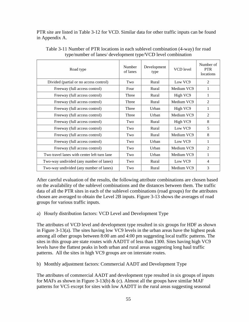
55
PTR site are listed in Table 3-12 for VCD. Similar data for other traffic inputs can be found
in Appendix A.
Table 3-11 Number of PTR locations in each sublevel combination (4-way) for road
type/number of lanes/ development type/VCD level combination
Road type Number
of lanes
Development
type VCD level
Number of
PTR
locations
Divided (partial or no access control) Two Rural Low VC9 2
Freeway (full access control) Four Rural Medium VC9 1
Freeway (full access control) Three Rural High VC9 1
Freeway (full access control) Three Rural Medium VC9 2
Freeway (full access control) Three Urban High VC9 1
Freeway (full access control) Three Urban Medium VC9 2
Freeway (full access control) Two Rural High VC9 8
Freeway (full access control) Two Rural Low VC9 5
Freeway (full access control) Two Rural Medium VC9 8
Freeway (full access control) Two Urban Low VC9 1
Freeway (full access control) Two Urban Medium VC9 2
Two travel lanes with center left turn lane Two Urban Medium VC9 1
Two-way undivided (any number of lanes) Two Rural Low VC9 4
Two-way undivided (any number of lanes) Two Rural Medium VC9 3
After careful evaluation of the results, the following attribute combinations are chosen based
on the availability of the sublevel combinations and the distances between them. The traffic
data of all the PTR sites in each of the sublevel combinations (road groups) for the attributes
chosen are averaged to obtain the Level 2B inputs. Figure 3-13 shows the averages of road
groups for various traffic inputs.
a) Hourly distribution factors: VCD Level and Development Type
The attributes of VCD level and development type resulted in six groups for HDF as shown
in Figure 3-13(a). The sites having low VC9 levels in the urban areas have the highest peak
among all other groups between 8:00 am and 4:00 pm suggesting local traffic patterns. The
sites in this group are state routes with AADTT of less than 1300. Sites having high VC9
levels have the flattest peaks in both urban and rural areas suggesting long haul traffic
patterns. All the sites in high VC9 groups are on interstate routes.
b) Monthly adjustment factors: Commercial AADT and Development Type
The attributes of commercial AADT and development type resulted in six groups of inputs
for MAFs as shown in Figure 3-13(b) & (c). Almost all the groups have similar MAF
patterns for VC5 except for sites with low AADTT in the rural areas suggesting seasonal
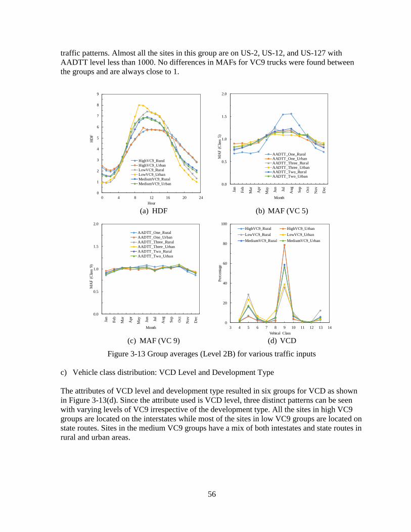
56
traffic patterns. Almost all the sites in this group are on US-2, US-12, and US-127 with
AADTT level less than 1000. No differences in MAFs for VC9 trucks were found between
the groups and are always close to 1.
(a) HDF
(b) MAF (VC 5)
(c) MAF (VC 9)
(d) VCD
Figure 3-13 Group averages (Level 2B) for various traffic inputs
c) Vehicle class distribution: VCD Level and Development Type
The attributes of VCD level and development type resulted in six groups for VCD as shown
in Figure 3-13(d). Since the attribute used is VCD level, three distinct patterns can be seen
with varying levels of VC9 irrespective of the development type. All the sites in high VC9
groups are located on the interstates while most of the sites in low VC9 groups are located on
state routes. Sites in the medium VC9 groups have a mix of both intestates and state routes in
rural and urban areas.
0
1
2
3
4
5
6
7
8
9
0 4 8 12 16 20 24
HD
F
Hour
HighVC9_Rural
HighVC9_Urban
LowVC9_Rural
LowVC9_Urban
MediumVC9_Rural
MediumVC9_Urban 0.0
0.5
1.0
1.5
2.0
Jan
Feb
Mar
Apr
May Jun
Jul
Aug
Sep
Oct
Nov
Dec
MA
F (
Cla
ss 5
)
Month
AADTT_One_RuralAADTT_One_UrbanAADTT_Three_RuralAADTT_Three_UrbanAADTT_Two_RuralAADTT_Two_Urban
0.0
0.5
1.0
1.5
2.0
Jan
Feb
Mar
Apr
May Jun
Jul
Aug
Sep
Oct
Nov
Dec
MA
F (
Cla
ss 9
)
Month
AADTT_One_Rural
AADTT_One_Urban
AADTT_Three_Rural
AADTT_Three_Urban
AADTT_Two_Rural
AADTT_Two_Urban
0
20
40
60
80
100
3 4 5 6 7 8 9 10 11 12 13 14
Per
cent
age
Vehical Class
HighVC9_Rural HighVC9_Urban
LowVC9_Rural LowVC9_Urban
MediumVC9_Rural MediumVC9_Urban
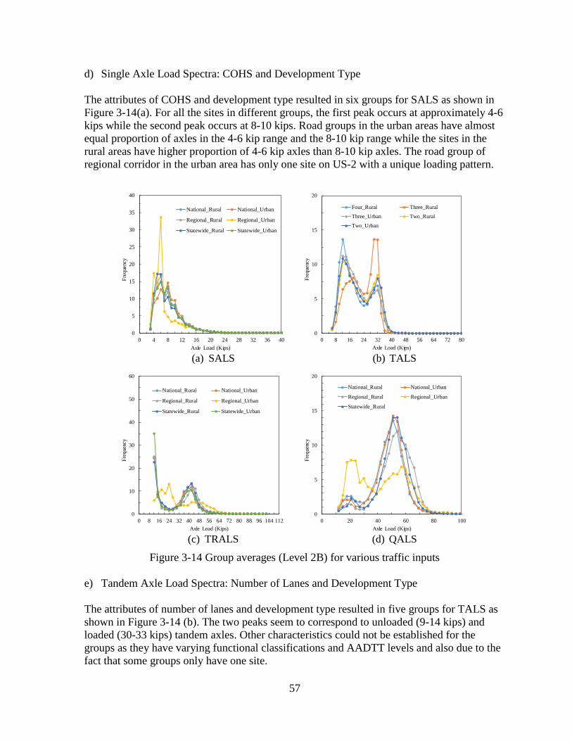
57
d) Single Axle Load Spectra: COHS and Development Type
The attributes of COHS and development type resulted in six groups for SALS as shown in
Figure 3-14(a). For all the sites in different groups, the first peak occurs at approximately 4-6
kips while the second peak occurs at 8-10 kips. Road groups in the urban areas have almost
equal proportion of axles in the 4-6 kip range and the 8-10 kip range while the sites in the
rural areas have higher proportion of 4-6 kip axles than 8-10 kip axles. The road group of
regional corridor in the urban area has only one site on US-2 with a unique loading pattern.
(a) SALS
(b) TALS
(c) TRALS
(d) QALS
Figure 3-14 Group averages (Level 2B) for various traffic inputs
e) Tandem Axle Load Spectra: Number of Lanes and Development Type
The attributes of number of lanes and development type resulted in five groups for TALS as
shown in Figure 3-14 (b). The two peaks seem to correspond to unloaded (9-14 kips) and
loaded (30-33 kips) tandem axles. Other characteristics could not be established for the
groups as they have varying functional classifications and AADTT levels and also due to the
fact that some groups only have one site.
0
5
10
15
20
25
30
35
40
0 4 8 12 16 20 24 28 32 36 40
Fre
que
ncy
Axle Load (Kips)
National_Rural National_Urban
Regional_Rural Regional_Urban
Statewide_Rural Statewide_Urban
0
5
10
15
20
0 8 16 24 32 40 48 56 64 72 80
Fre
que
ncy
Axle Load (Kips)
Four_Rural Three_Rural
Three_Urban Two_Rural
Two_Urban
0
10
20
30
40
50
60
0 8 16 24 32 40 48 56 64 72 80 88 96 104 112
Fre
que
ncy
Axle Load (Kips)
National_Rural National_Urban
Regional_Rural Regional_Urban
Statewide_Rural Statewide_Urban
0
5
10
15
20
0 20 40 60 80 100
Fre
que
ncy
Axle Load (Kips)
National_Rural National_Urban
Regional_Rural Regional_Urban
Statewide_Rural

58
f) Tridem Axle Load Spectra: COHS and Development Type
The attributes of COHS and development type resulted in six groups for TRALS as shown in
Figure 3-14 (c). The general trend of the tridem axle groups appears to be a large proportion
of light axles around 12 kips followed by a peak value around 40-45 kips. All the sites in the
national corridors are located on interstates while the sites on regional and statewide
corridors are on state routes with varying AADTT levels irrespective of the development
type.
g) Quad Axle Load Spectra: COHS and Development Type
The attributes of COHS and development type resulted in six groups for QALS as shown in
Figure 3-14 (d). Again, all the sites in national corridors are on the interstates while the sites
on regional and statewide corridors are on state routes with varying AADTT levels
irrespective of the development type.

59
Table 3-12 Descriptive Statistics of the pairwise distances between the sublevel combinations for various attribute combinations (VCD)
Attribute 1 Attribute 2
Pairwise Euclidean distances between the
sublevel combinations Sublevel combinations
Max Min Avg. Std. Range Total Available
With only
one PTR
location
Missing
VCD Level Development Type 50.0 1.5 26.5 15.1 48.5 6 6 0 0
Commercial AADT Development Type 46.8 1.9 21.3 11.9 44.9 6 6 0 0
COHS Development Type 28.3 2.9 18.0 7.1 25.4 6 6 1 0
Road Type Development Type 27.7 4.8 17.6 6.8 22.9 6 6 3 0
Functional Class Development Type 25.9 4.8 17.2 7.4 21.1 4 4 0 0
Functional Class VCD Level 50.4 6.7 25.5 14.4 43.7 6 5 0 1
Number of Lanes Development Type 41.6 4.3 19.0 16.1 37.3 6 5 2 1
Functional Class Commercial AADT 40.2 5.4 21.1 11.5 34.8 6 5 0 1
Functional Class COHS 28.7 8.0 15.9 6.7 20.7 6 5 0 1
COHS VCD Level 54.5 2.5 23.0 13.2 52.1 9 7 1 2
Commercial AADT VCD Level 50.3 1.9 24.3 14.3 48.4 9 7 0 2
Commercial AADT COHS 42.0 4.2 22.0 11.9 37.9 9 7 1 2
Road Type COHS 28.7 2.1 16.1 7.7 26.7 9 7 3 2
Functional Class Number of Lanes 28.0 6.9 15.8 7.8 21.2 6 4 1 2
Road Type VCD Level 56.1 7.6 25.3 14.0 48.5 9 6 0 3
Number of Lanes VCD Level 53.2 1.7 23.9 14.7 51.4 9 6 1 3
Road Type Commercial AADT 42.7 5.4 21.0 10.9 37.3 9 6 0 3
Number of Lanes Commercial AADT 42.3 1.1 18.1 11.0 41.1 9 6 1 3
Functional Class Road Type 23.1 9.7 17.8 7.2 13.5 6 3 0 3
Road Type Number of Lanes 28.8 6.9 16.4 7.5 22.0 9 5 1 4
Number of Lanes COHS 26.1 5.5 14.9 7.0 20.6 9 5 1 4
Note: Shaded cells indicate the selected attribute combination for generation of Level 2B inputs

60
3.3 SUMMARY
This chapter discussed the permanent traffic recorder (PTR) data collection and processing
for developing traffic input defaults for the Pavement-ME. Site-specific traffic inputs (Level
1) were generated for each of the 41 WIM sites using the PrepME software after applying
QC checks. Development of Level 2 inputs is crucial when site-specific data are not
available. The averages from clusters or groups with similar traffic characteristics can be
used as Level 2 data (2). The average of all the sites (statewide average) can be used as Level
3 data. Level 3 data are further divided into Levels 3A, and 3B, where 3A represents average
traffic inputs of freeways and non-freeways, and 3B represents overall statewide average for
traffic inputs. Two approaches were used to develop Level 2 traffic inputs (a) cluster
analyses (i.e., improved existing approach) and (b) traditional approaches (simplified
methodology).
The advantages of cluster analyses are that the groups are formed objectively (based on a
mathematical function) and not subjected to bias or subjective decisions. In addition, it finds
patterns in the data that are not intuitively obvious therefore providing new insights into
traffic patterns in a region. One main disadvantage is the lack of guidelines on establishing
the optimal number of clusters. While various techniques were developed to identify the
optimal number of clusters, none of them are perfect and have their drawbacks. The other
disadvantage is that, since clustering is purely a mathematical technique, the sites in a cluster
might not have the same identifiable attributes making the assignment of data from a new
location to the existing clusters difficult. The Euclidean distance and Ward’s method were
used as the similarity measure and the linkage method, respectively to cluster the traffic data.
‘Calinski-Harbasz Criterion’ and ‘Gap Criterion’ methods , and engineering judgements were
used to determine the optimal number of clusters for each traffic input. The inputs developed
using this methodology are identified as ‘Level 2A’ inputs in this report.
Traditional approaches are more subjective and involve grouping roads that are expected to
behave similarly (i.e., similar traffic patterns). Attributes of the roadways (e.g., road class
freeway vs. non-freeway) can be used to identify groups that have similar traffic patterns.
Such groups based on these attributes are easy to interpret by the users. A minimum of three
to six groups are required, but more groups may be appropriate if significant regional
differences exist (3). The advantages of this methodology are that the creation of groups is
intuitive, and the short-term count from a new site can be used to assign it to an existing
group. The drawback of this process is that it is not entirely objective (involves a lot of
subjective decisions which may not explain the variability of traffic patterns within a group).
Also, the challenge lies in identifying a combination of attributes that can be used to group
the PTR locations. The traffic patterns at the PTR locations should be similar within a group
and should be different between the groups. An automated process was developed to help
identify such combinations of attributes. The inputs developed using this methodology are
called ‘Level 2B’ inputs in this report.

61
The traffic input levels developed in this study are listed below.
a. Level 1 – Site-specific inputs
b. Level 2A – Averages of clusters based on cluster analyses
c. Level 2B – Averages of groups based on roadway characteristics (attributes)
d. Level 3A – Averages of groups based on freeway and non-freeway road class
e. Level 3B – Statewide averages
Table 3-13 lists the number of clusters and road groups formed that could be used as Level 2
traffic inputs.
Table 3-13 Number of clusters and road groups formed for Level 2 inputs
Input
Number of
clusters
(Level 2A)
Road groups
(Level 2B)
Hourly distribution factors (HDF) 5 6
Monthly adjustment factors (MAF) based on VC 5 4 6
MAF based on VC9 5 6
Vehicle class distribution (VCD) 5 6
Single axle load spectra (SALS) 4 6
Tandem axle load spectra (TALS) 5 5
Tridem axle load spectra (TRALS) 6 6
Quad axle load spectra (QALS) 3 6

62
CHAPTER 4 - SIGNIFICANT TRAFFIC INPUTS
In Chapter 3, the Pavement-ME traffic inputs were generated for Levels 1, 2A, 2B, 3A and
3B. Level 1 inputs should always be used for design purposes wherever possible as it is the
actual traffic data specific to the site. When Level 1 inputs are unavailable, Level 2 or Level
3 inputs need to be used. The results of the sensitivity analyses based on statistical
significance and maximum life difference should be used to decide on the appropriate traffic
input level. The primary purpose of sensitivity analyses is to identify if the traffic defaults
developed based on clustering (Level 2A inputs) or road grouping (Level 2B inputs)
techniques would provide significantly different pavement life predictions. The statewide
defaults (Level 3A or 3B inputs) would suffice for some of the traffic inputs for which the
Level 2 inputs do not have a significant impact on pavement design outcomes. The steps
involved in sensitivity analyses include establishing base designs, performance criteria and
other input parameters in the Pavement-ME and then evaluating the impact of Levels 2 and 3
traffic inputs.
The impact of Level 2 inputs on pavement designs can be evaluated in two ways:
Option 1: Changing one input at a time to Level 2 and keeping all other inputs at Level 1, this
sensitivity analyses is referred to as Option 1.
Option 2: Changing one input at a time to Level 2 and keeping all other inputs at Level 3, this
sensitivity analyses is referred to as Option 2.
In Option 1, the impact of input Level 2 is relative to site-specific traffic characteristics (i.e.,
Level 1). On the other hand, in Option 2 the effect of Level 2 is relative to the statewide
traffic characteristics (i.e., Level 3). Option 2 will isolate the impact of a single traffic input
because only one traffic input was changed to Level 2 and all other inputs were kept at Level
3. Option 1 is more realistic since site-specific traffic data are used except for the Level 2
input for each WIM location. However, Option 2 was included since the most States have
adopted such approaches.
4.1 SENSITIVITY ANALYSES – OPTION 1
Table 4-1 contains the baseline flexible pavement design used for the sensitivity analyses.
Material inputs used in these designs were as per MDOT guidance. The Pavement-ME
Version 2.3 was used for the sensitivity analysis. For both the flexible and rigid pavements,
locally calibrated performance models were used with only one climate station in Lansing
(1, 2) (see Appendix B). The pavement design life was assumed 20 years with 95% design
reliability. For each of the 41 WIM locations, the HMA surface layer thickness was designed
to achieve a 20-year design life for bottom-up fatigue cracking threshold of 20% for flexible
pavements since it typically controls the designs. Level 1 inputs were used in this process.
For these designs, the rut depth values at the end of 20 years were also recorded. Table 4-2
presents the baseline rigid pavement design used for the sensitivity analyses. For each of the
41 WIM locations, the slab thickness was designed to achieve a 20-year design life for IRI

63
threshold of 172 inches/mile since it controls the designs for rigid pavements. Faulting and
transverse cracking values were also recorded at the end of 20 years.
For both the flexible and rigid pavement designs, one traffic input was changed at a time to
appropriate cluster or road groups for the site of the PTR. (Levels 2A and 2B) to determine
the effect of that input on the design life. Levels 3A and 3B inputs for each design (one input
at a time) were also tested in the Pavement-ME to determine their impact on the design life.
The time for the distress values (for Levels 2 and 3) to reach the threshold values in the Level
1 designs were documented. The differences in design lives between different inputs levels
were quantified for further analyses.
Table 4-1 Baseline designs for flexible pavements
Layer/Detail Elastic Modulus (psi) Thickness (in)
Asphalt Estimated by the Pavement-ME Variable
Aggregate base (A-1-a) 33000 6
Sand subbase-A-1-b 20000 18
Sandy clay subgrade-A4 4400 Semi-Infinite
Climate Lansing, MI
Table 4-2 Baseline designs for rigid pavements
Layer/Detail Elastic Modulus (psi) Thickness (in)
JPCP 5600 ('
cf ) Variable
Open graded base (A-1-a) 33000 6
Sand subbase (A-1-b) 20000 10
Sandy clay roadbed (A-6) 4400 Semi-Infinite
Joint spacing 15 ft.
Dowel bar diameter 1.25 in (<10in) 1.5in (=>10in)
Climate Lansing, MI
Many statistical analyses can be performed to understand the characteristics of a data set and
differences between datasets. Statistical analyses could detect differences in the datasets, but
the differences might not have much practical significance or vice versa. Statistically,
significant differences can be found even with minimal differences between datasets of
considerable size. That is, a statistical significance of the results does not always imply
practical consequence. Hence in addition to finding the likelihood of a value (significance
value ‘ ’) outside the 95% confidence interval (CI), the maximum life difference (MLD)
values between two input levels were also adopted as an indicator of the variability in the
data. The MLD is the maximum difference in life between traffic input levels among the PTR
locations. Table 4-3 lists the criteria used to determine the impact (sensitivity) of the
difference between traffic inputs and correspondingly select the proper input level needed for
the design. These designations will be used to measure each traffic characterization
performance against site-specific values and to determine its impact on life differences.
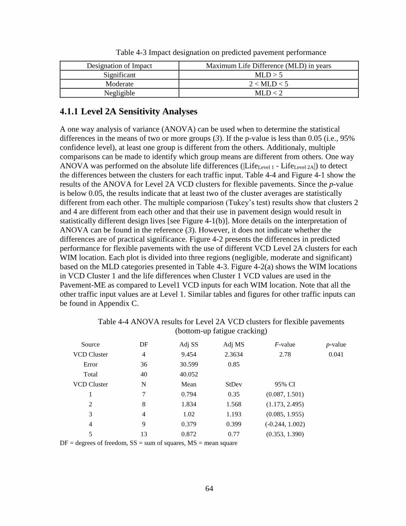
64
Table 4-3 Impact designation on predicted pavement performance
Designation of Impact Maximum Life Difference (MLD) in years
Significant MLD > 5
Moderate 2 < MLD < 5
Negligible MLD < 2
4.1.1 Level 2A Sensitivity Analyses
A one way analysis of variance (ANOVA) can be used when to determine the statistical
differences in the means of two or more groups (3). If the p-value is less than 0.05 (i.e., 95%
confidence level), at least one group is different from the others. Additionaly, multiple
comparisons can be made to identify which group means are different from others. One way
ANOVA was performed on the absolute life differences (|LifeLevel 1 - LifeLevel 2A|) to detect
the differences between the clusters for each traffic input. Table 4-4 and Figure 4-1 show the
results of the ANOVA for Level 2A VCD clusters for flexible pavements. Since the p-value
is below 0.05, the results indicate that at least two of the cluster averages are statistically
different from each other. The multiple compariosn (Tukey’s test) results show that clusters 2
and 4 are different from each other and that their use in pavement design would result in
statistically different design lives [see Figure 4-1(b)]. More details on the interpretation of
ANOVA can be found in the reference (3). However, it does not indicate whether the
differences are of practical significance. Figure 4-2 presents the differences in predicted
performance for flexible pavements with the use of different VCD Level 2A clusters for each
WIM location. Each plot is divided into three regions (negligible, moderate and significant)
based on the MLD categories presented in Table 4-3. Figure 4-2(a) shows the WIM locations
in VCD Cluster 1 and the life differences when Cluster 1 VCD values are used in the
Pavement-ME as compared to Level1 VCD inputs for each WIM location. Note that all the
other traffic input values are at Level 1. Similar tables and figures for other traffic inputs can
be found in Appendix C.
Table 4-4 ANOVA results for Level 2A VCD clusters for flexible pavements
(bottom-up fatigue cracking)
Source DF Adj SS Adj MS F-value p-value
VCD Cluster 4 9.454 2.3634 2.78 0.041
Error 36 30.599 0.85
Total 40 40.052
VCD Cluster N Mean StDev 95% CI
1 7 0.794 0.35 (0.087, 1.501)
2 8 1.834 1.568 (1.173, 2.495)
3 4 1.02 1.193 (0.085, 1.955)
4 9 0.379 0.399 (-0.244, 1.002)
5 13 0.872 0.77 (0.353, 1.390)
DF = degrees of freedom, SS = sum of squares, MS = mean square
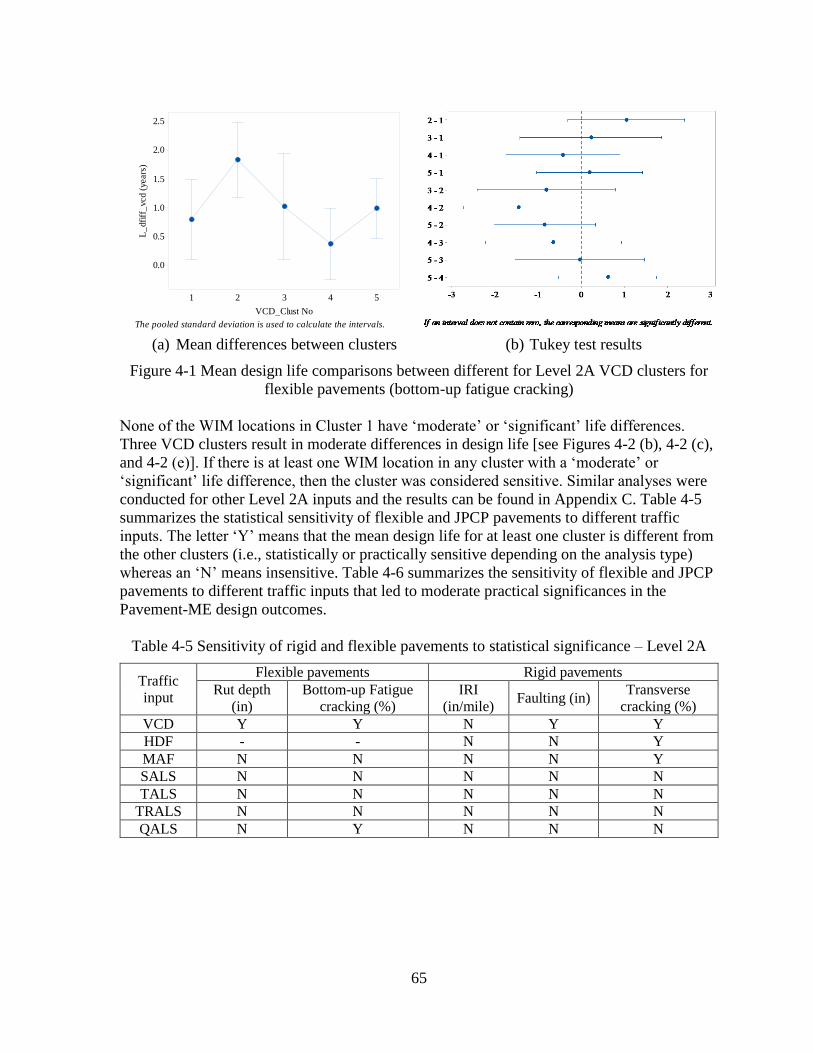
65
(a) Mean differences between clusters
(b) Tukey test results
Figure 4-1 Mean design life comparisons between different for Level 2A VCD clusters for
flexible pavements (bottom-up fatigue cracking)
None of the WIM locations in Cluster 1 have ‘moderate’ or ‘significant’ life differences.
Three VCD clusters result in moderate differences in design life [see Figures 4-2 (b), 4-2 (c),
and 4-2 (e)]. If there is at least one WIM location in any cluster with a ‘moderate’ or
‘significant’ life difference, then the cluster was considered sensitive. Similar analyses were
conducted for other Level 2A inputs and the results can be found in Appendix C. Table 4-5
summarizes the statistical sensitivity of flexible and JPCP pavements to different traffic
inputs. The letter ‘Y’ means that the mean design life for at least one cluster is different from
the other clusters (i.e., statistically or practically sensitive depending on the analysis type)
whereas an ‘N’ means insensitive. Table 4-6 summarizes the sensitivity of flexible and JPCP
pavements to different traffic inputs that led to moderate practical significances in the
Pavement-ME design outcomes.
Table 4-5 Sensitivity of rigid and flexible pavements to statistical significance – Level 2A
Traffic
input
Flexible pavements Rigid pavements
Rut depth
(in)
Bottom-up Fatigue
cracking (%)
IRI
(in/mile) Faulting (in)
Transverse
cracking (%)
VCD Y Y N Y Y
HDF - - N N Y
MAF N N N N Y
SALS N N N N N
TALS N N N N N
TRALS N N N N N
QALS N Y N N N
54321
2.5
2.0
1.5
1.0
0.5
0.0
VCD_Clust No
L_
dfi
ff_
vcd (
years
)
The pooled standard deviation is used to calculate the intervals.
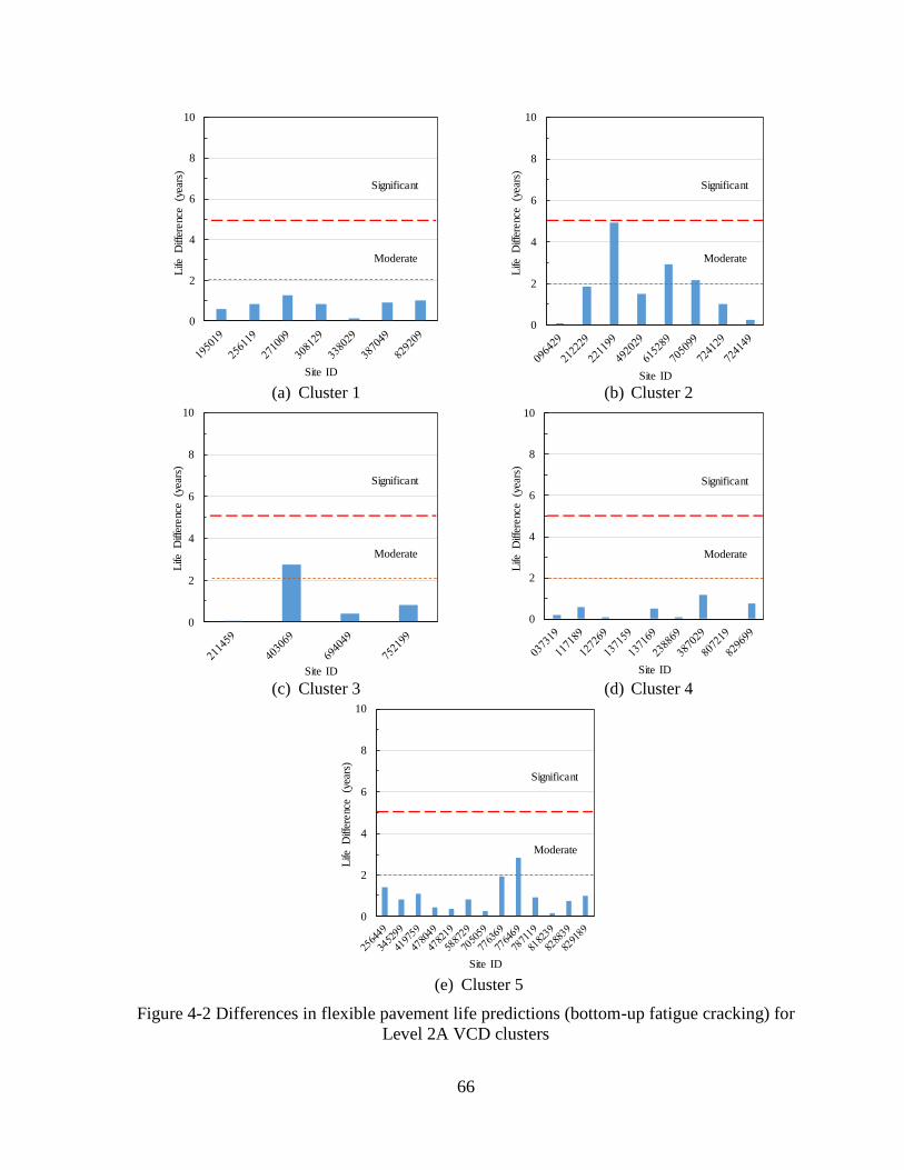
66
(a) Cluster 1
(b) Cluster 2
(c) Cluster 3
(d) Cluster 4
(e) Cluster 5
Figure 4-2 Differences in flexible pavement life predictions (bottom-up fatigue cracking) for
Level 2A VCD clusters
0
2
4
6
8
10
Life
D
iffer
enc
e (y
ears
)
Site ID
Significant
Moderate
0
2
4
6
8
10
Life
D
iffer
enc
e (y
ears
)
Site ID
Significant
Moderate
0
2
4
6
8
10
Life
D
iffer
enc
e (y
ears
)
Site ID
Significant
Moderate
0
2
4
6
8
10
Life
D
iffer
enc
e (y
ears
)
Site ID
Significant
Moderate
0
2
4
6
8
10
Life
D
iffer
enc
e (y
ears
)
Site ID
Significant
Moderate
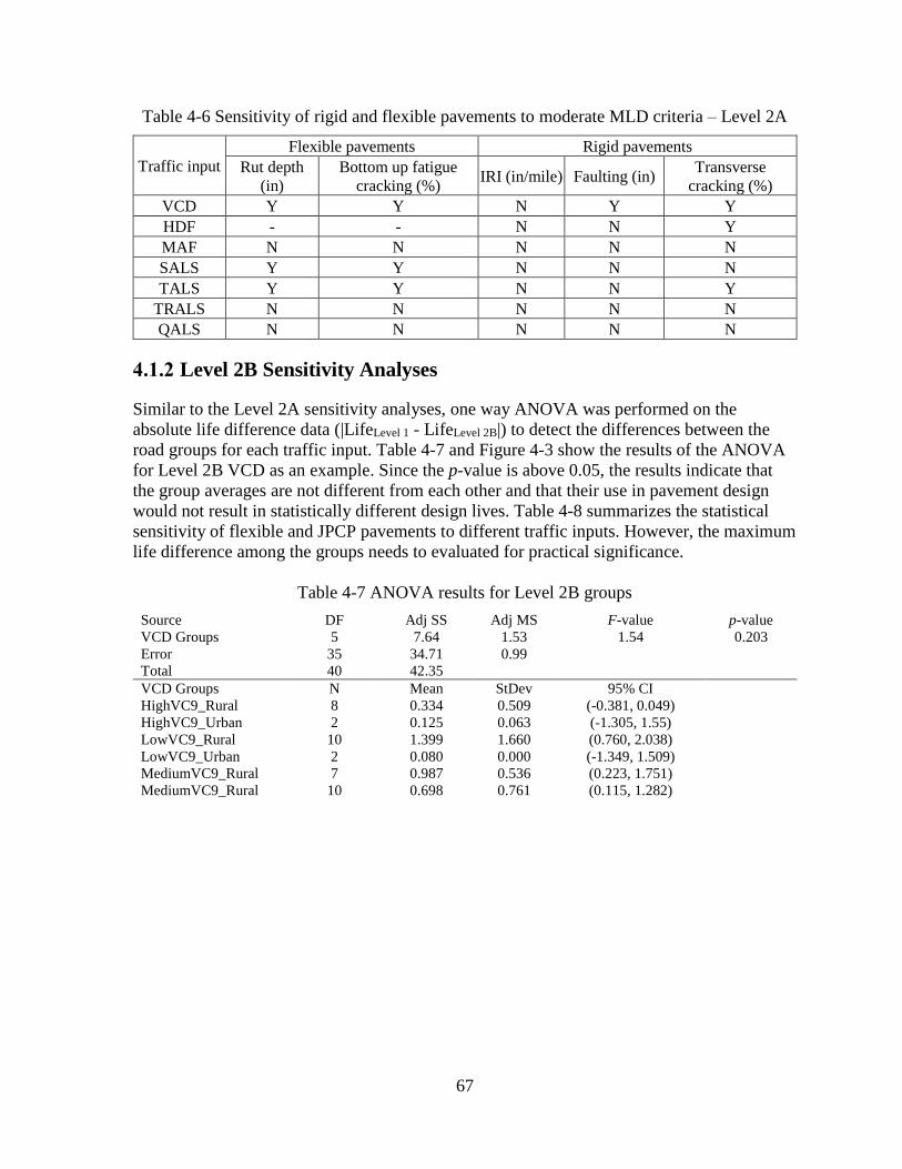
67
Table 4-6 Sensitivity of rigid and flexible pavements to moderate MLD criteria – Level 2A
Traffic input
Flexible pavements Rigid pavements
Rut depth
(in)
Bottom up fatigue
cracking (%) IRI (in/mile) Faulting (in)
Transverse
cracking (%)
VCD Y Y N Y Y
HDF - - N N Y
MAF N N N N N
SALS Y Y N N N
TALS Y Y N N Y
TRALS N N N N N
QALS N N N N N
4.1.2 Level 2B Sensitivity Analyses
Similar to the Level 2A sensitivity analyses, one way ANOVA was performed on the
absolute life difference data (|LifeLevel 1 - LifeLevel 2B|) to detect the differences between the
road groups for each traffic input. Table 4-7 and Figure 4-3 show the results of the ANOVA
for Level 2B VCD as an example. Since the p-value is above 0.05, the results indicate that
the group averages are not different from each other and that their use in pavement design
would not result in statistically different design lives. Table 4-8 summarizes the statistical
sensitivity of flexible and JPCP pavements to different traffic inputs. However, the maximum
life difference among the groups needs to evaluated for practical significance.
Table 4-7 ANOVA results for Level 2B groups
Source DF Adj SS Adj MS F-value p-value
VCD Groups 5 7.64 1.53 1.54 0.203
Error 35 34.71 0.99
Total 40 42.35
VCD Groups N Mean StDev 95% CI
HighVC9_Rural 8 0.334 0.509 (-0.381, 0.049)
HighVC9_Urban 2 0.125 0.063 (-1.305, 1.55)
LowVC9_Rural 10 1.399 1.660 (0.760, 2.038)
LowVC9_Urban 2 0.080 0.000 (-1.349, 1.509)
MediumVC9_Rural 7 0.987 0.536 (0.223, 1.751)
MediumVC9_Rural 10 0.698 0.761 (0.115, 1.282)
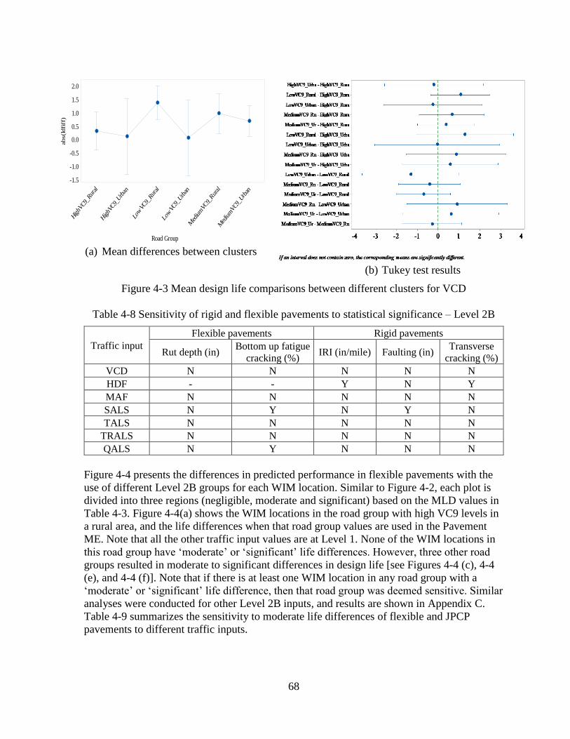
68
(a) Mean differences between clusters
(b) Tukey test results
Figure 4-3 Mean design life comparisons between different clusters for VCD
Table 4-8 Sensitivity of rigid and flexible pavements to statistical significance – Level 2B
Traffic input
Flexible pavements Rigid pavements
Rut depth (in) Bottom up fatigue
cracking (%) IRI (in/mile) Faulting (in)
Transverse
cracking (%)
VCD N N N N N
HDF - - Y N Y
MAF N N N N N
SALS N Y N Y N
TALS N N N N N
TRALS N N N N N
QALS N Y N N N
Figure 4-4 presents the differences in predicted performance in flexible pavements with the
use of different Level 2B groups for each WIM location. Similar to Figure 4-2, each plot is
divided into three regions (negligible, moderate and significant) based on the MLD values in
Table 4-3. Figure 4-4(a) shows the WIM locations in the road group with high VC9 levels in
a rural area, and the life differences when that road group values are used in the Pavement
ME. Note that all the other traffic input values are at Level 1. None of the WIM locations in
this road group have ‘moderate’ or ‘significant’ life differences. However, three other road
groups resulted in moderate to significant differences in design life [see Figures 4-4 (c), 4-4
(e), and 4-4 (f)]. Note that if there is at least one WIM location in any road group with a
‘moderate’ or ‘significant’ life difference, then that road group was deemed sensitive. Similar
analyses were conducted for other Level 2B inputs, and results are shown in Appendix C.
Table 4-9 summarizes the sensitivity to moderate life differences of flexible and JPCP
pavements to different traffic inputs.
Med
iumVC9
_Urb
an
Med
iumVC
9_Rural
LowVC
9_Urban
LowVC
9_Rur
al
HighV
C9_Urban
HighV
C9_R
ural
2.0
1.5
1.0
0.5
0.0
-0.5
-1.0
-1.5
Road Group
abs(l
dfi
ff)

69
(a) High VC9 and Rural
(b) High VC9 and Urban
(c) Low VC9 and Rural
(d) Low VC9 and Urban
(e) Medium VC9 and Rural
(f) Medium VC9 and Urban
Figure 4-4 Differences in flexible pavement life predictions (bottom-up fatigue cracking)
for Level 2B VCD road groups
0
2
4
6
8
10
Life
D
iffer
enc
e (y
ears
)
Site ID
Significant
Moderate
0
2
4
6
8
10
807219 829699
Life
D
iffer
enc
e (y
ears
)
Site ID
Significant
Moderate
0
2
4
6
8
10
Life
D
iffer
enc
e (y
ears
)
Site ID
Significant
Moderate
0
2
4
6
8
10
Life
D
iffer
enc
e (y
ears
)
Site ID
Significant
Moderate
0
2
4
6
8
10
Life
D
iffer
enc
e (y
ears
)
Site ID
Significant
Moderate
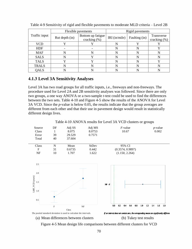
70
Table 4-9 Sensitivity of rigid and flexible pavements to moderate MLD criteria – Level 2B
Traffic input
Flexible pavements Rigid pavements
Rut depth (in) Bottom up fatigue
cracking (%) IRI (in/mile) Faulting (in)
Transverse
cracking (%)
VCD Y Y N Y Y
HDF - - N N Y
MAF N N N N N
SALS N Y N N N
TALS Y Y N N Y
TRALS N N N N N
QALS N N N N N
4.1.3 Level 3A Sensitivity Analyses
Level 3A has two road groups for all traffic inputs, i.e., freeways and non-freeways. The
procedure used for Level 2A and 2B sensitivity analyses was followed. Since there are only
two groups, a one way ANOVA or a two-sample t-test could be used to find the differences
between the two sets. Table 4-10 and Figure 4-5 show the results of the ANOVA for Level
3A VCD. Since the p-value is below 0.05, the results indicate that the group averages are
different from each other and that their use in pavement design would result in statistically
different design lives.
Table 4-10 ANOVA results for Level 3A VCD clusters or groups
Source DF Adj SS Adj MS F-value p-value
Class 1 8.075 8.0753 10.67 0.002
Error 39 29.529 0.7571
Total 40 37.604
Class N Mean StDev 95% CI
F 31 0.6735 0.442 (0.3574, 0.9897)
NF 10 1.707 1.622 (1.150, 2.264)
(a) Mean differences between clusters
(b) Tukey test results
Figure 4-5 Mean design life comparisons between different clusters for VCD
NFF
2.5
2.0
1.5
1.0
0.5
Class
Ldif
f_V
CD
(years
)
The pooled standard deviation is used to calculate the intervals.
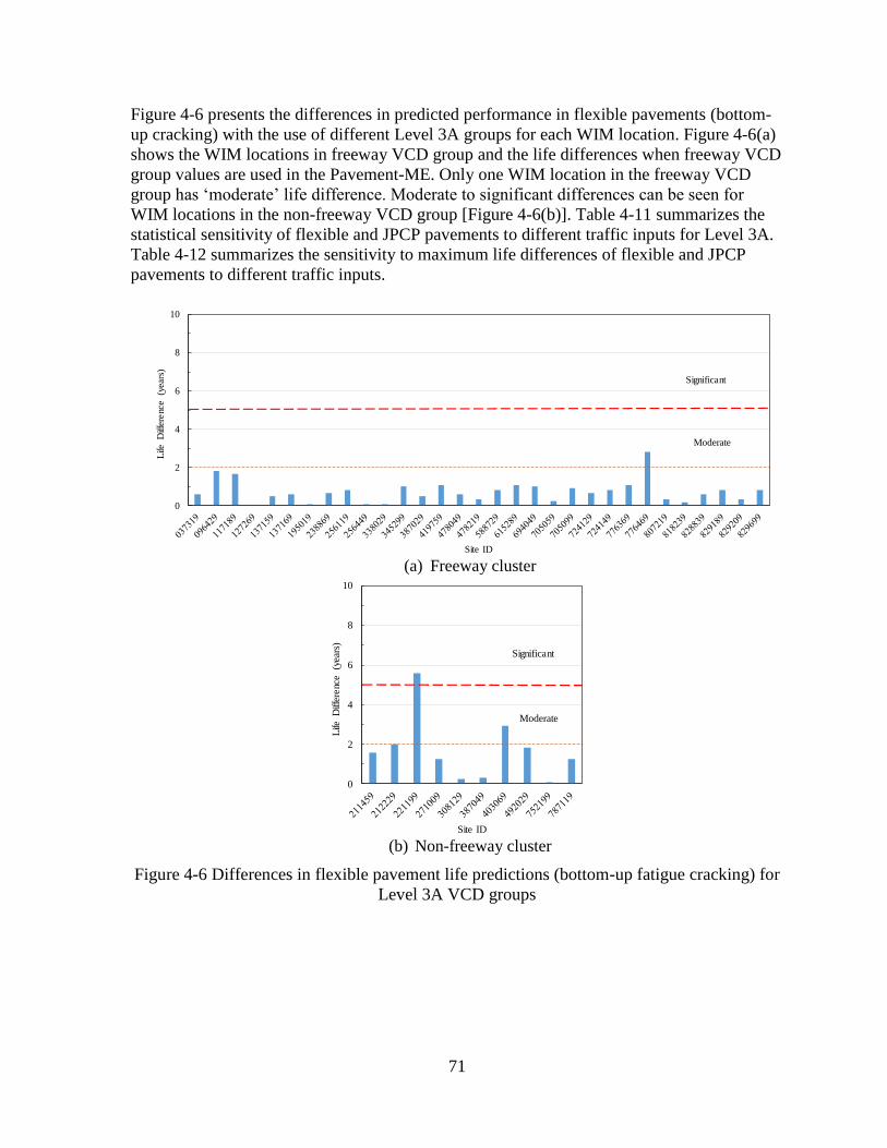
71
Figure 4-6 presents the differences in predicted performance in flexible pavements (bottom-
up cracking) with the use of different Level 3A groups for each WIM location. Figure 4-6(a)
shows the WIM locations in freeway VCD group and the life differences when freeway VCD
group values are used in the Pavement-ME. Only one WIM location in the freeway VCD
group has ‘moderate’ life difference. Moderate to significant differences can be seen for
WIM locations in the non-freeway VCD group [Figure 4-6(b)]. Table 4-11 summarizes the
statistical sensitivity of flexible and JPCP pavements to different traffic inputs for Level 3A.
Table 4-12 summarizes the sensitivity to maximum life differences of flexible and JPCP
pavements to different traffic inputs.
(a) Freeway cluster
(b) Non-freeway cluster
Figure 4-6 Differences in flexible pavement life predictions (bottom-up fatigue cracking) for
Level 3A VCD groups
0
2
4
6
8
10
Life
D
iffer
enc
e (y
ears
)
Site ID
Significant
Moderate
0
2
4
6
8
10
Life
D
iffer
enc
e (y
ears
)
Site ID
Significant
Moderate

72
Table 4-11 Sensitivity of rigid and flexible pavements to statistical significance – Level 3A
Traffic
Input
Flexible pavements Rigid pavements
Rut depth
(in)
Bottom-up fatigue
cracking (%)
IRI
(in/mile) Faulting (in)
Transverse
cracking (%)
VCD Y Y N N N
HDF - - N N N
MAF N N N N Y
SALS N Y N N N
TALS N Y N Y N
TRALS N Y N N N
QALS N N N N N
Table 4-12 Sensitivity of rigid and flexible pavements to MLD criteria – Level 3A
Traffic
Input
Flexible pavements Rigid pavements
Rut depth (in) Bottom-up fatigue
cracking (%)
IRI
(in/mile)
Faulting
(in)
Transverse
cracking (%)
VCD Y Y N Y Y
HDF - - N N Y
MAF N N N N Y
SALS N Y N N Y
TALS Y N N N Y
TRALS N N N N N
QALS N N N N N
4.1.4 Choosing the Appropriate Traffic Input Level
As mentioned before, Level 1 traffic inputs should always be used for pavement design if
available. In the absence of Level 1 inputs, use either Level 2 or Level 3 inputs. The results
of the sensitivity analyses based on statistical significance and maximum life difference
should be used to decide on the appropriate traffic input level. The criteria used in this
evaluation is that the traffic input levels are sensitive if the life difference is moderate (> 2
years). The recommendations for each traffic input are as follows:
4.1.4.1 Vehicle class distribution
The statistical sensitivity analyses show that the use of different VCD clusters (Level 2A)
would result in statistically different design lives for both flexible and rigid pavements (see
Table 4-5). This observation is also valid for MLD sensitivity analyses. The results indicate
the existence of localized traffic patterns that would yield different pavement thicknesses in
the design process. While the statistical analyses do not show that Level 2B inputs would
result in statistically different design lives for both flexible and rigid pavements, the MLD
criteria indicate that the use of Level 2B inputs would result in moderate life differences.
Hence, for VCD, either Level 2A or 2B inputs could be used in the absence of Level 1
inputs. The next step is to identify if there are any statistical differences between Levels 2A
and 2B. If there are no differences between the two levels, then Level 2B can be used since it
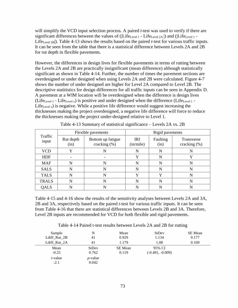
73
will simplify the VCD input selection process. A paired t-test was used to verify if there are
significant differences between the values of (|LifeLevel 1 - LifeLevel 2A |) and (|LifeLevel 1 -
LifeLevel 2B|). Table 4-13 shows the results based on the paired t-test for various traffic inputs.
It can be seen from the table that there is a statistical difference between Levels 2A and 2B
for rut depth in flexible pavements.
However, the differences in design lives for flexible pavements in terms of rutting between
the Levels 2A and 2B are practically insignificant (mean difference) although statistically
significant as shown in Table 4-14. Further, the number of times the pavement sections are
overdesigned or under designed when using Levels 2A and 2B were calculated. Figure 4-7
shows the number of under designed are higher for Level 2A compared to Level 2B. The
descriptive statitistics for design differences for all traffic inputs can be seen in Appendix D.
A pavement at a WIM location will be overdesigned when the difference is design lives
(LifeLevel 1 - LifeLevel x) is positive and under designed when the difference (LifeLevel 1 -
LifeLevel x) is negative. While a positive life difference would suggest increasing the
thicknesses making the project overdesigned, a negative life difference will force to reduce
the thicknesses making the project under-designed relative to Level 1.
Table 4-13 Summary of statistical significance – Levels 2A vs. 2B
Traffic
input
Flexible pavements Rigid pavements
Rut depth
(in)
Bottom up fatigue
cracking (%)
IRI
(in/mile)
Faulting
(in)
Transverse
cracking (%)
VCD Y N N N N
HDF - - Y N Y
MAF N N N N N
SALS N N N N N
TALS N N Y Y N
TRALS N N N N N
QALS N N N N N
Table 4-15 and 4-16 show the results of the sensitivity analyses between Levels 2A and 3A,
2B and 3A, respectively based on the paired t-test for various traffic inputs. It can be seen
from Table 4-16 that there are statistical differences between Levels 2B and 3A. Therefore,
Level 2B inputs are recommended for VCD for both flexible and rigid pavements.
Table 4-14 Paired t-test results between Levels 2A and 2B for rutting
Sample N Mean StDev SE Mean
Ldiff_Rut_2B 41 0.929 1.134 0.177
Ldiff_Rut_2A 41 1.179 1.08 0.169
Mean StDev SE Mean 95% CI
-0.25 0.762 0.119 (-0.491, -0.009) t-value p-value
-2.1 0.042
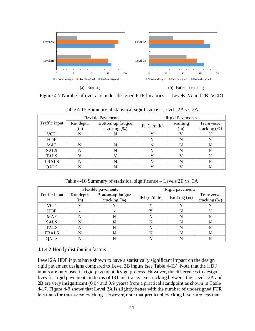
74
(a) Rutting
(b) Fatigue cracking
Figure 4-7 Number of over and under-designed PTR locations — Levels 2A and 2B (VCD)
Table 4-15 Summary of statistical significance – Levels 2A vs. 3A
Traffic input
Flexible Pavements Rigid Pavements
Rut depth
(in)
Bottom-up fatigue
cracking (%) IRI (in/mile)
Faulting
(in)
Transverse
cracking (%)
VCD N N Y Y Y
HDF - - N N Y
MAF N N N N N
SALS N N N N N
TALS Y Y Y Y Y
TRALS N N N N N
QALS N N Y Y N
Table 4-16 Summary of statistical significance – Levels 2B vs. 3A
Traffic input
Flexible pavements Rigid pavements
Rut depth
(in)
Bottom-up fatigue
cracking (%) IRI (in/mile) Faulting (in)
Transverse
cracking (%)
VCD Y Y Y Y Y
HDF - - Y N Y
MAF N N N N N
SALS N N N N N
TALS N N N N N
TRALS N N N N N
QALS N N N N N
4.1.4.2 Hourly distribution factors
Level 2A HDF inputs have shown to have a statistically significant impact on the design
rigid pavement designs compared to Level 2B inputs (see Table 4-13). Note that the HDF
inputs are only used in rigid pavement design process. However, the differences in design
lives for rigid pavements in terms of IRI and transverse cracking between the Levels 2A and
2B are very insignificant (0.04 and 0.9 years) from a practical standpoint as shown in Table
4-17. Figure 4-8 shows that Level 2A is slightly better with the number of undersigned PTR
locations for transverse cracking. However, note that predicted cracking levels are less than
0 5 10 15 20
Level 2B
Level 2A
Normal design Overdesigned Underdesigned
0 5 10 15 20
Level 2B
Level 2A
Normal design Overdesigned Underdesigned
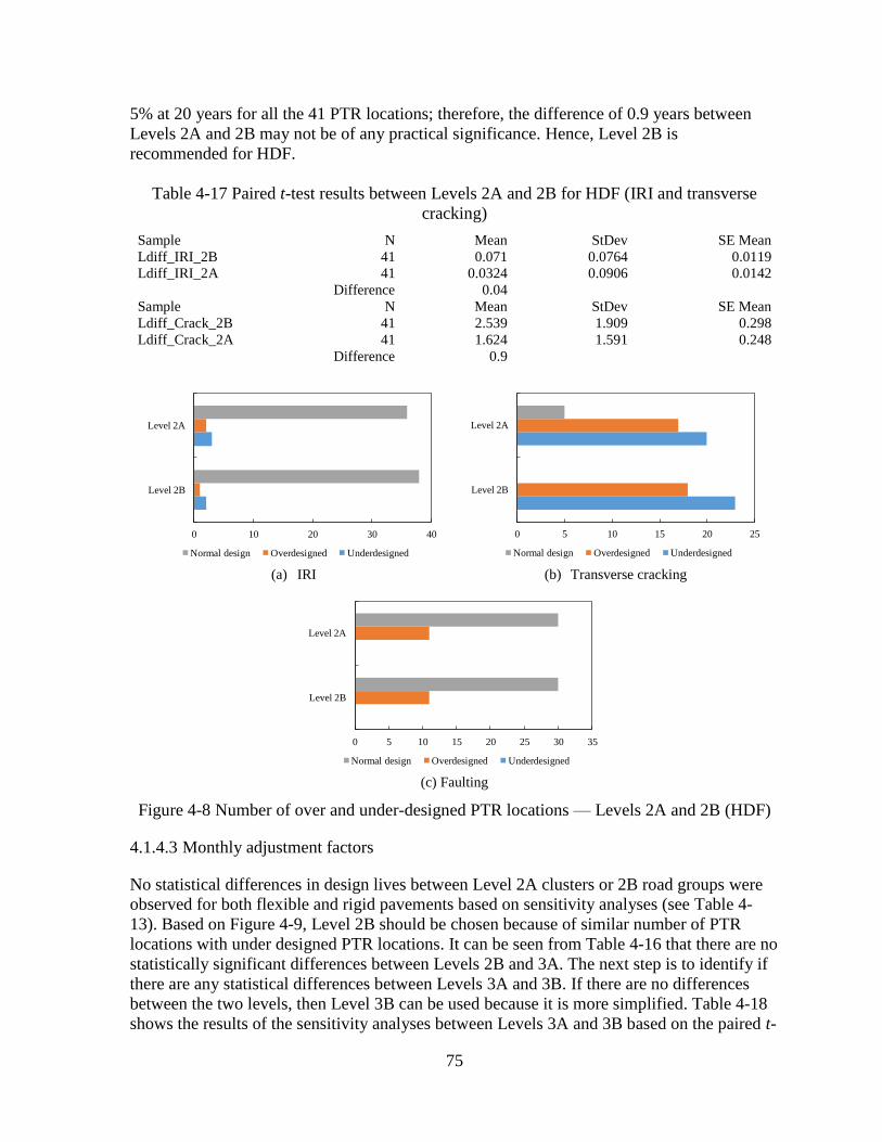
75
5% at 20 years for all the 41 PTR locations; therefore, the difference of 0.9 years between
Levels 2A and 2B may not be of any practical significance. Hence, Level 2B is
recommended for HDF.
Table 4-17 Paired t-test results between Levels 2A and 2B for HDF (IRI and transverse
cracking)
Sample N Mean StDev SE Mean
Ldiff_IRI_2B 41 0.071 0.0764 0.0119
Ldiff_IRI_2A 41 0.0324 0.0906 0.0142
Difference 0.04
Sample N Mean StDev SE Mean
Ldiff_Crack_2B 41 2.539 1.909 0.298
Ldiff_Crack_2A 41 1.624 1.591 0.248
Difference 0.9
(a) IRI
(b) Transverse cracking
(c) Faulting
Figure 4-8 Number of over and under-designed PTR locations — Levels 2A and 2B (HDF)
4.1.4.3 Monthly adjustment factors
No statistical differences in design lives between Level 2A clusters or 2B road groups were
observed for both flexible and rigid pavements based on sensitivity analyses (see Table 4-
13). Based on Figure 4-9, Level 2B should be chosen because of similar number of PTR
locations with under designed PTR locations. It can be seen from Table 4-16 that there are no
statistically significant differences between Levels 2B and 3A. The next step is to identify if
there are any statistical differences between Levels 3A and 3B. If there are no differences
between the two levels, then Level 3B can be used because it is more simplified. Table 4-18
shows the results of the sensitivity analyses between Levels 3A and 3B based on the paired t-
0 10 20 30 40
Level 2B
Level 2A
Normal design Overdesigned Underdesigned
0 5 10 15 20 25
Level 2B
Level 2A
Normal design Overdesigned Underdesigned
0 5 10 15 20 25 30 35
Level 2B
Level 2A
Normal design Overdesigned Underdesigned
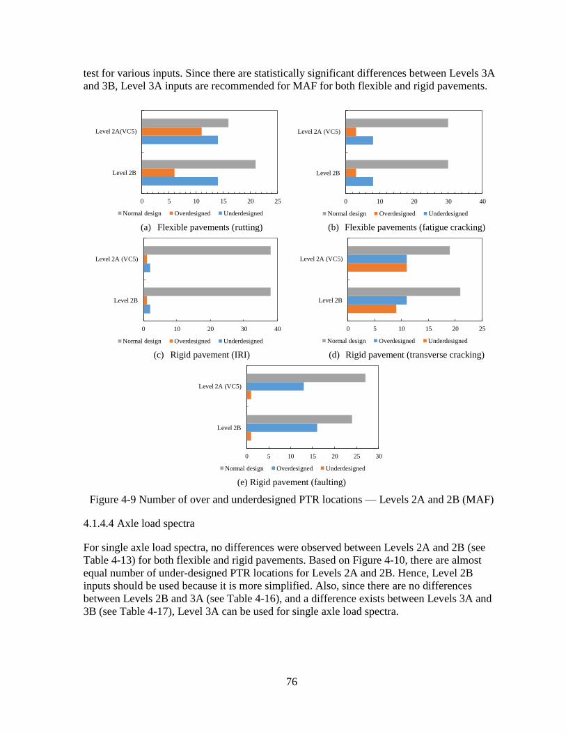
76
test for various inputs. Since there are statistically significant differences between Levels 3A
and 3B, Level 3A inputs are recommended for MAF for both flexible and rigid pavements.
(a) Flexible pavements (rutting)
(b) Flexible pavements (fatigue cracking)
(c) Rigid pavement (IRI)
(d) Rigid pavement (transverse cracking)
(e) Rigid pavement (faulting)
Figure 4-9 Number of over and underdesigned PTR locations — Levels 2A and 2B (MAF)
4.1.4.4 Axle load spectra
For single axle load spectra, no differences were observed between Levels 2A and 2B (see
Table 4-13) for both flexible and rigid pavements. Based on Figure 4-10, there are almost
equal number of under-designed PTR locations for Levels 2A and 2B. Hence, Level 2B
inputs should be used because it is more simplified. Also, since there are no differences
between Levels 2B and 3A (see Table 4-16), and a difference exists between Levels 3A and
3B (see Table 4-17), Level 3A can be used for single axle load spectra.
0 5 10 15 20 25
Level 2B
Level 2A(VC5)
Normal design Overdesigned Underdesigned
0 10 20 30 40
Level 2B
Level 2A (VC5)
Normal design Overdesigned Underdesigned
0 10 20 30 40
Level 2B
Level 2A (VC5)
Normal design Overdesigned Underdesigned
0 5 10 15 20 25
Level 2B
Level 2A (VC5)
Normal design Overdesigned Underdesigned
0 5 10 15 20 25 30
Level 2B
Level 2A (VC5)
Normal design Overdesigned Underdesigned
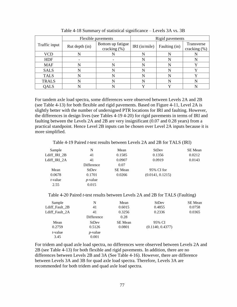
77
Table 4-18 Summary of statistical significance – Levels 3A vs. 3B
Traffic input
Flexible pavements Rigid pavements
Rut depth (in) Bottom up fatigue
cracking (%) IRI (in/mile) Faulting (in)
Transverse
cracking (%)
VCD N N N N N
HDF - - N N N
MAF N N N N Y
SALS N N N N Y
TALS N N N N Y
TRALS N N N N N
QALS N N Y Y N
For tandem axle load spectra, some differences were observed between Levels 2A and 2B
(see Table 4-13) for both flexible and rigid pavements. Based on Figure 4-11, Level 2A is
slightly better with the number of undersigned PTR locations for IRI and faulting. However,
the differences in design lives (see Tables 4-19 4-20) for rigid pavements in terms of IRI and
faulting between the Levels 2A and 2B are very insignificant (0.07 and 0.28 years) from a
practical standpoint. Hence Level 2B inputs can be chosen over Level 2A inputs because it is
more simplified.
Table 4-19 Paired t-test results between Levels 2A and 2B for TALS (IRI)
Sample N Mean StDev SE Mean
Ldiff_IRI_2B 41 0.1585 0.1356 0.0212
Ldiff_IRI_2A 41 0.0907 0.0919 0.0143
Difference 0.07
Mean StDev SE Mean 95% CI for
0.0678 0.1701 0.0266 (0.0141, 0.1215)
t-value p-value
2.55 0.015
Table 4-20 Paired t-test results between Levels 2A and 2B for TALS (Faulting)
Sample N Mean StDev SE Mean
Ldiff_Fault_2B 41 0.6015 0.4855 0.0758
Ldiff_Fault_2A 41 0.3256 0.2336 0.0365
Difference 0.28
Mean StDev SE Mean 95% CI
0.2759 0.5126 0.0801 (0.1140, 0.4377) t-value p-value
3.45 0.001
For tridem and quad axle load spectra, no differences were observed between Levels 2A and
2B (see Table 4-13) for both flexible and rigid pavements. In addition, there are no
differences between Levels 2B and 3A (See Table 4-16). However, there are difference
between Levels 3A and 3B for quad axle load spectra. Therefore, Levels 3A are
recommended for both tridem and quad axle load spectra.
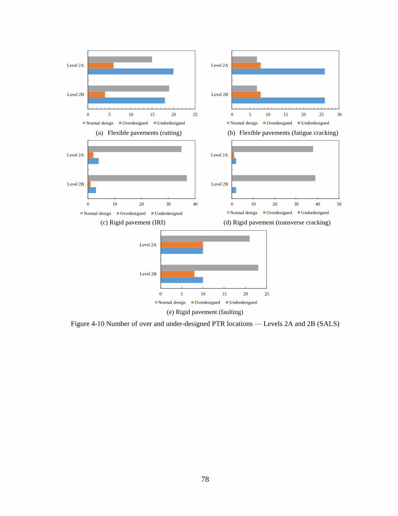
78
(a) Flexible pavements (rutting)
(b) Flexible pavements (fatigue cracking)
(c) Rigid pavement (IRI)
(d) Rigid pavement (transverse cracking)
(e) Rigid pavement (faulting)
Figure 4-10 Number of over and under-designed PTR locations — Levels 2A and 2B (SALS)
0 5 10 15 20 25
Level 2B
Level 2A
Normal design Overdesigned Underdesigned
0 5 10 15 20 25 30
Level 2B
Level 2A
Normal design Overdesigned Underdesigned
0 10 20 30 40
Level 2B
Level 2A
Normal design Overdesigned Underdesigned
0 10 20 30 40 50
Level 2B
Level 2A
Normal design Overdesigned Underdesigned
0 5 10 15 20 25
Level 2B
Level 2A
Normal design Overdesigned Underdesigned
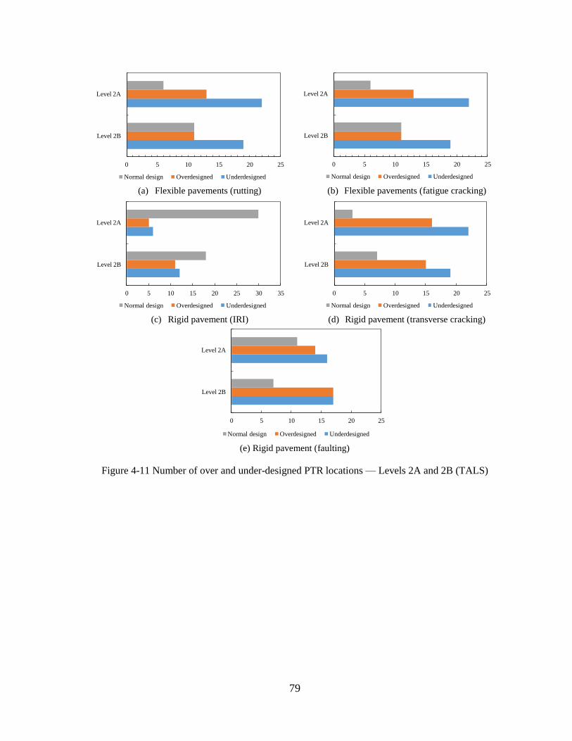
79
(a) Flexible pavements (rutting)
(b) Flexible pavements (fatigue cracking)
(c) Rigid pavement (IRI)
(d) Rigid pavement (transverse cracking)
(e) Rigid pavement (faulting)
Figure 4-11 Number of over and under-designed PTR locations — Levels 2A and 2B (TALS)
0 5 10 15 20 25
Level 2B
Level 2A
Normal design Overdesigned Underdesigned
0 5 10 15 20 25
Level 2B
Level 2A
Normal design Overdesigned Underdesigned
0 5 10 15 20 25 30 35
Level 2B
Level 2A
Normal design Overdesigned Underdesigned
0 5 10 15 20 25
Level 2B
Level 2A
Normal design Overdesigned Underdesigned
0 5 10 15 20 25
Level 2B
Level 2A
Normal design Overdesigned Underdesigned
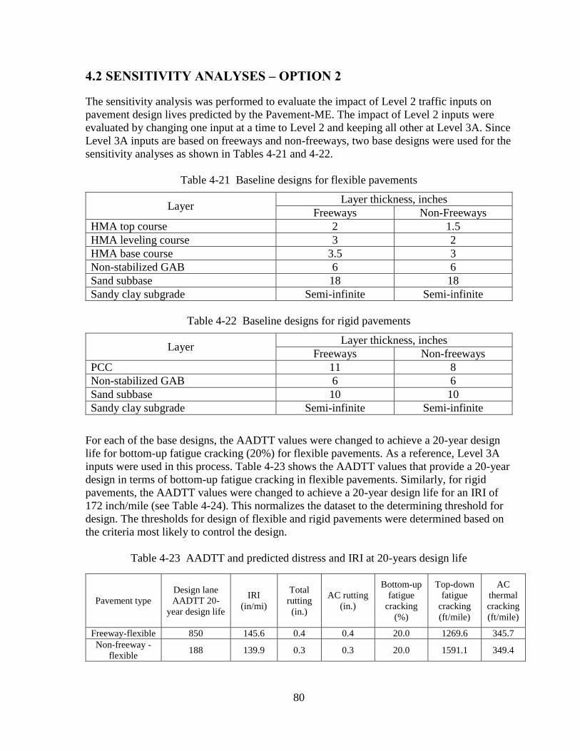
80
4.2 SENSITIVITY ANALYSES – OPTION 2
The sensitivity analysis was performed to evaluate the impact of Level 2 traffic inputs on
pavement design lives predicted by the Pavement-ME. The impact of Level 2 inputs were
evaluated by changing one input at a time to Level 2 and keeping all other at Level 3A. Since
Level 3A inputs are based on freeways and non-freeways, two base designs were used for the
sensitivity analyses as shown in Tables 4-21 and 4-22.
Table 4-21 Baseline designs for flexible pavements
Layer Layer thickness, inches
Freeways Non-Freeways
HMA top course 2 1.5
HMA leveling course 3 2
HMA base course 3.5 3
Non-stabilized GAB 6 6
Sand subbase 18 18
Sandy clay subgrade Semi-infinite Semi-infinite
Table 4-22 Baseline designs for rigid pavements
Layer Layer thickness, inches
Freeways Non-freeways
PCC 11 8
Non-stabilized GAB 6 6
Sand subbase 10 10
Sandy clay subgrade Semi-infinite Semi-infinite
For each of the base designs, the AADTT values were changed to achieve a 20-year design
life for bottom-up fatigue cracking (20%) for flexible pavements. As a reference, Level 3A
inputs were used in this process. Table 4-23 shows the AADTT values that provide a 20-year
design in terms of bottom-up fatigue cracking in flexible pavements. Similarly, for rigid
pavements, the AADTT values were changed to achieve a 20-year design life for an IRI of
172 inch/mile (see Table 4-24). This normalizes the dataset to the determining threshold for
design. The thresholds for design of flexible and rigid pavements were determined based on
the criteria most likely to control the design.
Table 4-23 AADTT and predicted distress and IRI at 20-years design life
Pavement type
Design lane
AADTT 20-
year design life
IRI
(in/mi)
Total
rutting
(in.)
AC rutting
(in.)
Bottom-up
fatigue
cracking
(%)
Top-down
fatigue
cracking
(ft/mile)
AC
thermal
cracking
(ft/mile)
Freeway-flexible 850 145.6 0.4 0.4 20.0 1269.6 345.7
Non-freeway -
flexible 188 139.9 0.3 0.3 20.0 1591.1 349.4

81
Table 4-24 AADTT and predicted distress and IRI at 20-year design life
Pavement type
Design lane
AADTT 20-year
design life
IRI
(in/mi)
Mean joint
faulting
(in)
JPCP transverse
cracking (percent
slabs)
Freeway- rigid 525 172.9 0.1 0.7
Non-freeway - rigid 500 172.4 0.0 2.9
Once the baseline designs are established, one input at a time were changed to Level 2
keeping all the other inputs at Level 3A. The time it takes for the pavement sections to reach
the threshold limit of 20 percent bottom-up fatigue cracking for flexible pavements and 172
inch/mile IRI for rigid pavements were determined.
4.2.1 Level 2A Sensitivity Analyses
4.2.1.1 Vehicle Class Distribution
Tables 4-25 and 4-26 demonstrate the results of the sensitivity analysis of five VCD clusters
(Level 2A) inputs. Since the percent difference in design life is less than 2 years for both
freeways and non-freeways and for all clusters, it can be concluded that VCD clusters have
little to no practical effect on the design life and Level 3A inputs will suffice for VCD for
flexible and rigid pavement designs.
Table 4-25 Effects of VCD Level 2A inputs on flexible pavements performance
Clusters Years to
failure
IRI
(in/mi)
Total
rutting
(in.)
AC
rutting
(in.)
Bottom-
up fatigue
cracking
(%)
Top-
down
fatigue
cracking
(ft/mile)
AC
thermal
cracking
(ft/mile)
%
Difference
in design
life
Freeway-Flexible-
Baseline 20.0 145.60 0.43 0.4 20.0 1,270 345.7 -
Cluster 1 20.7 145.30 0.43 0.4 19.9 1,275 345.7 3%
Cluster 2 18.9 146.10 0.44 0.4 20.4 1,340 345.7 -5%
Cluster 3 20.0 145.30 0.43 0.4 20.0 1,296 345.7 0%
Cluster 4 20.0 145.80 0.43 0.4 20.0 1,240 345.7 0%
Cluster 5 20.1 145.60 0.43 0.4 20.0 1,263 345.7 0%
Non-Freeway -
Flexible-Baseline 20.0 139.90 0.34 0.3 20.0 1,591 349.4 -
Cluster 1 21.8 139.40 0.33 0.3 19.6 1,551 349.4 9%
Cluster 2 19.9 140.10 0.34 0.3 20.1 1,621 349.4 0%
Cluster 3 20.9 139.50 0.33 0.3 19.7 1,562 349.4 5%
Cluster 4 20.8 139.90 0.34 0.3 19.9 1,559 349.4 4%
Cluster 5 20.9 139.70 0.33 0.3 19.7 1,559 349.4 5%
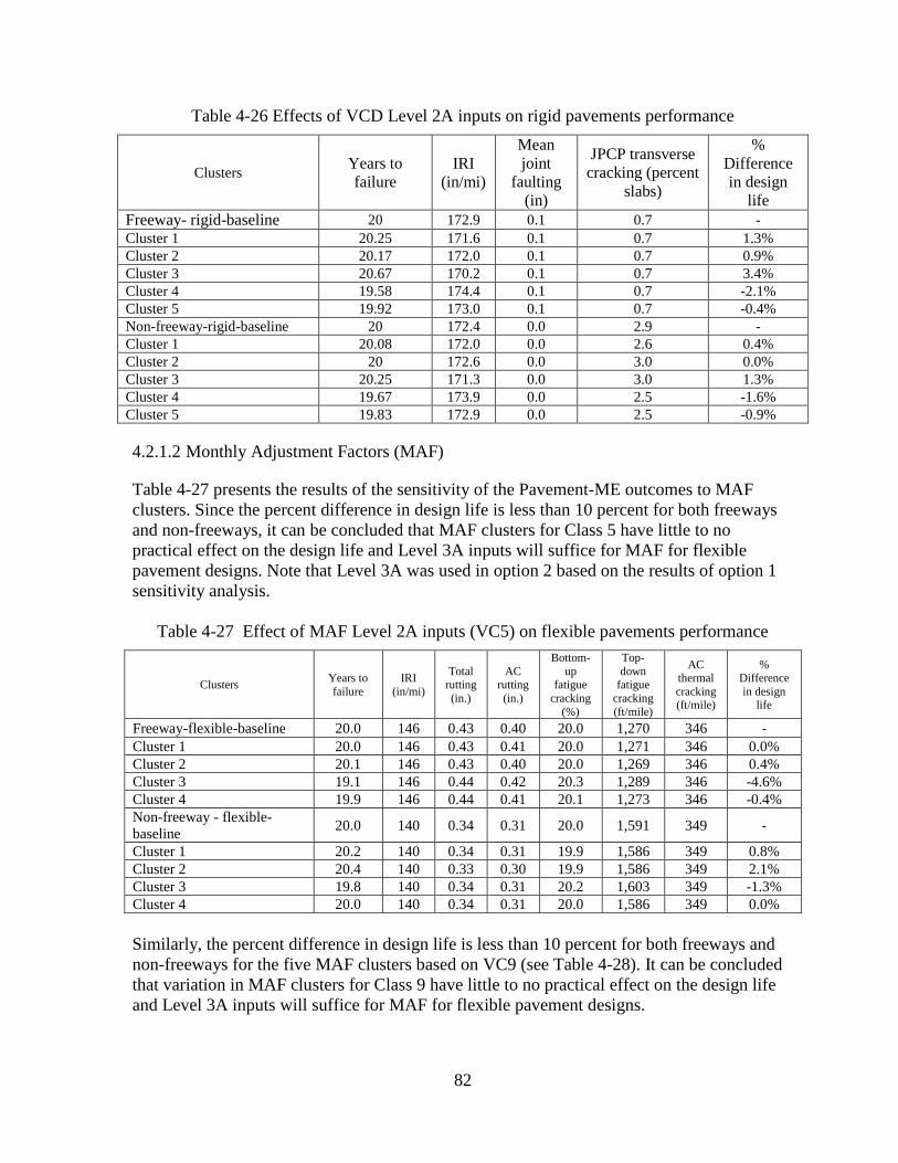
82
Table 4-26 Effects of VCD Level 2A inputs on rigid pavements performance
Clusters Years to
failure
IRI
(in/mi)
Mean
joint
faulting
(in)
JPCP transverse
cracking (percent
slabs)
%
Difference
in design
life
Freeway- rigid-baseline 20 172.9 0.1 0.7 -
Cluster 1 20.25 171.6 0.1 0.7 1.3%
Cluster 2 20.17 172.0 0.1 0.7 0.9%
Cluster 3 20.67 170.2 0.1 0.7 3.4%
Cluster 4 19.58 174.4 0.1 0.7 -2.1%
Cluster 5 19.92 173.0 0.1 0.7 -0.4%
Non-freeway-rigid-baseline 20 172.4 0.0 2.9 -
Cluster 1 20.08 172.0 0.0 2.6 0.4%
Cluster 2 20 172.6 0.0 3.0 0.0%
Cluster 3 20.25 171.3 0.0 3.0 1.3%
Cluster 4 19.67 173.9 0.0 2.5 -1.6%
Cluster 5 19.83 172.9 0.0 2.5 -0.9%
4.2.1.2 Monthly Adjustment Factors (MAF)
Table 4-27 presents the results of the sensitivity of the Pavement-ME outcomes to MAF
clusters. Since the percent difference in design life is less than 10 percent for both freeways
and non-freeways, it can be concluded that MAF clusters for Class 5 have little to no
practical effect on the design life and Level 3A inputs will suffice for MAF for flexible
pavement designs. Note that Level 3A was used in option 2 based on the results of option 1
sensitivity analysis.
Table 4-27 Effect of MAF Level 2A inputs (VC5) on flexible pavements performance
Clusters Years to
failure
IRI
(in/mi)
Total rutting
(in.)
AC rutting
(in.)
Bottom-
up fatigue
cracking
(%)
Top-
down fatigue
cracking
(ft/mile)
AC thermal
cracking (ft/mile)
% Difference
in design life
Freeway-flexible-baseline 20.0 146 0.43 0.40 20.0 1,270 346 - Cluster 1 20.0 146 0.43 0.41 20.0 1,271 346 0.0%
Cluster 2 20.1 146 0.43 0.40 20.0 1,269 346 0.4%
Cluster 3 19.1 146 0.44 0.42 20.3 1,289 346 -4.6%
Cluster 4 19.9 146 0.44 0.41 20.1 1,273 346 -0.4%
Non-freeway - flexible-
baseline 20.0 140 0.34 0.31 20.0 1,591 349 -
Cluster 1 20.2 140 0.34 0.31 19.9 1,586 349 0.8%
Cluster 2 20.4 140 0.33 0.30 19.9 1,586 349 2.1%
Cluster 3 19.8 140 0.34 0.31 20.2 1,603 349 -1.3%
Cluster 4 20.0 140 0.34 0.31 20.0 1,586 349 0.0%
Similarly, the percent difference in design life is less than 10 percent for both freeways and
non-freeways for the five MAF clusters based on VC9 (see Table 4-28). It can be concluded
that variation in MAF clusters for Class 9 have little to no practical effect on the design life
and Level 3A inputs will suffice for MAF for flexible pavement designs.
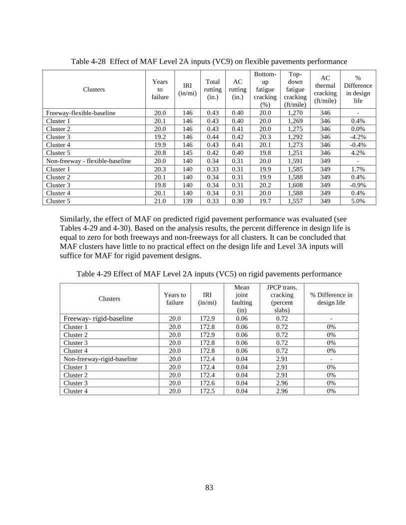
83
Table 4-28 Effect of MAF Level 2A inputs (VC9) on flexible pavements performance
Clusters
Years
to
failure
IRI
(in/mi)
Total
rutting
(in.)
AC
rutting
(in.)
Bottom-
up
fatigue
cracking
(%)
Top-
down
fatigue
cracking
(ft/mile)
AC
thermal
cracking
(ft/mile)
%
Difference
in design
life
Freeway-flexible-baseline 20.0 146 0.43 0.40 20.0 1,270 346 - Cluster 1 20.1 146 0.43 0.40 20.0 1,269 346 0.4%
Cluster 2 20.0 146 0.43 0.41 20.0 1,275 346 0.0%
Cluster 3 19.2 146 0.44 0.42 20.3 1,292 346 -4.2%
Cluster 4 19.9 146 0.43 0.41 20.1 1,273 346 -0.4%
Cluster 5 20.8 145 0.42 0.40 19.8 1,251 346 4.2%
Non-freeway - flexible-baseline 20.0 140 0.34 0.31 20.0 1,591 349 - Cluster 1 20.3 140 0.33 0.31 19.9 1,585 349 1.7%
Cluster 2 20.1 140 0.34 0.31 19.9 1,588 349 0.4%
Cluster 3 19.8 140 0.34 0.31 20.2 1,608 349 -0.9%
Cluster 4 20.1 140 0.34 0.31 20.0 1,588 349 0.4%
Cluster 5 21.0 139 0.33 0.30 19.7 1,557 349 5.0%
Similarly, the effect of MAF on predicted rigid pavement performance was evaluated (see
Tables 4-29 and 4-30). Based on the analysis results, the percent difference in design life is
equal to zero for both freeways and non-freeways for all clusters. It can be concluded that
MAF clusters have little to no practical effect on the design life and Level 3A inputs will
suffice for MAF for rigid pavement designs.
Table 4-29 Effect of MAF Level 2A inputs (VC5) on rigid pavements performance
Clusters Years to
failure
IRI
(in/mi)
Mean
joint
faulting
(in)
JPCP trans.
cracking
(percent
slabs)
% Difference in
design life
Freeway- rigid-baseline 20.0 172.9 0.06 0.72 -
Cluster 1 20.0 172.8 0.06 0.72 0%
Cluster 2 20.0 172.9 0.06 0.72 0%
Cluster 3 20.0 172.8 0.06 0.72 0%
Cluster 4 20.0 172.8 0.06 0.72 0%
Non-freeway-rigid-baseline 20.0 172.4 0.04 2.91 - Cluster 1 20.0 172.4 0.04 2.91 0%
Cluster 2 20.0 172.4 0.04 2.91 0%
Cluster 3 20.0 172.6 0.04 2.96 0%
Cluster 4 20.0 172.5 0.04 2.96 0%

84
Table 4-30 Effect of MAF Level 2A inputs (VC9) on rigid pavements performance
Clusters
Years
to
failure
IRI
(in/mi)
Mean joint
faulting (in)
JPCP
transverse
cracking
(percent slabs)
% Difference in
design life
Freeway- rigid-baseline 20.0 172.9 0.06 0.72 -
Cluster 1 20.0 172.8 0.06 0.72 0.0%
Cluster 2 20.0 172.8 0.06 0.72 0.0%
Cluster 3 20.0 172.9 0.06 0.72 0.0%
Cluster 4 20.0 172.9 0.06 0.72 0.0%
Cluster 5 19.9 173.3 0.06 0.72 -0.4%
Non-freeway-rigid-baseline 20.0 172.4 0.04 2.91 -
Cluster 1 20.0 172.4 0.04 2.91 0.0%
Cluster 2 20.0 172.4 0.04 2.91 0.0%
Cluster 3 20.0 172.6 0.04 2.96 0.0%
Cluster 4 20.0 172.5 0.04 2.96 0.0%
Cluster 5 20.0 172.4 0.04 2.82 0.0%
4.2.1.3 Hourly Distribution Factors (HDF)
The effect of five Level 2 HDF clusters on the Pavement-ME rigid pavement design was
investigated. Based on the analysis results, the percent difference in design life is equal to
zero (see Table 4-31) for all clusters and for both freeways and non-freeways. It can be
concluded that HDF clusters have little to no practical effect on the design life and Level 3A
inputs will suffice for HDF for rigid pavement designs.
Table 4-31 Effect of HDF Level 2A inputs on rigid pavements performance
Clusters Years to
failure
IRI
(in/mi)
Mean joint
faulting (in)
JPCP transverse
cracking (percent
slabs)
% Difference
in design life
Freeway-rigid-baseline 20.0 172.9 0.06 0.72 -
Cluster 1 20.0 172.9 0.06 0.72 0.0%
Cluster 2 20.0 172.9 0.06 0.72 0.0%
Cluster 3 20.0 172.9 0.06 0.72 0.0%
Cluster 4 20.0 172.9 0.06 0.72 0.0%
Cluster 5 20.0 172.9 0.06 0.96 0.0%
Non-freeway-rigid-baseline 20.0 172.4 0.04 2.91 -
Cluster 1 20.0 172.5 0.04 3.05 0.0%
Cluster 2 20.0 172.5 0.04 2.96 0.0%
Cluster 3 20.0 172.5 0.04 3.05 0.0%
Cluster 4 20.0 172.4 0.04 2.87 0.0%
Cluster 5 20.0 172.6 0.04 3.18 0.0%
4.2.1.4 Axle Load Spectra (ALS)
The effect of Level 2A clusters on pavement performance was evaluated in terms of predicted
pavement service life using the baseline designs. Four single and five tandem Level 2A ALS
cluster inputs were tested. The results are presented in Table 4-32. Since the percent difference
in design life is less than 10 percent for both freeways and non-freeways, it can be concluded
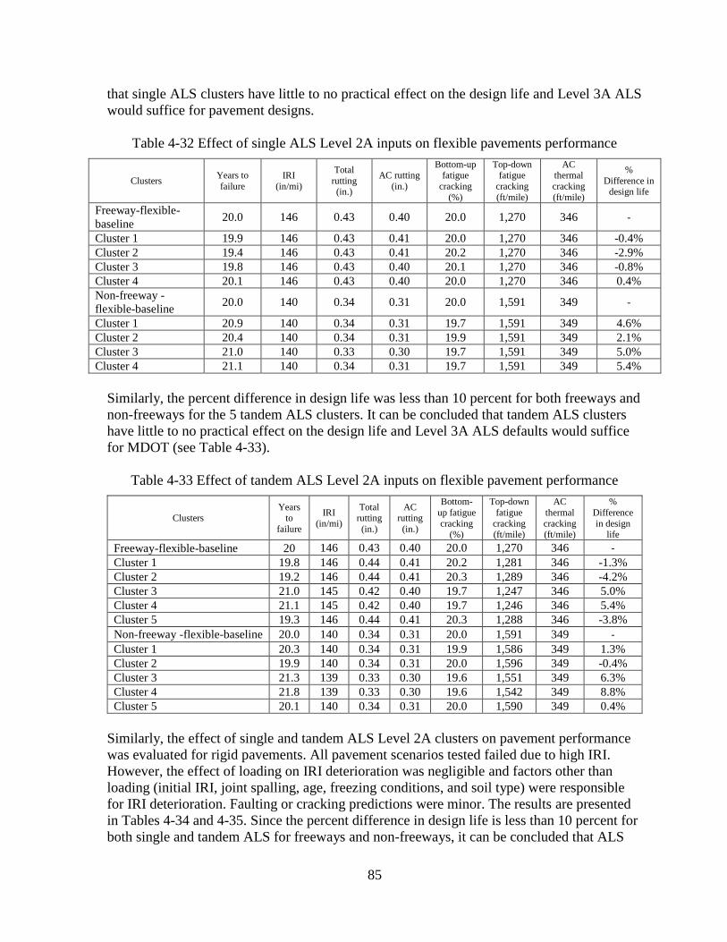
85
that single ALS clusters have little to no practical effect on the design life and Level 3A ALS
would suffice for pavement designs.
Table 4-32 Effect of single ALS Level 2A inputs on flexible pavements performance
Clusters Years to
failure
IRI
(in/mi)
Total
rutting (in.)
AC rutting
(in.)
Bottom-up fatigue
cracking
(%)
Top-down fatigue
cracking
(ft/mile)
AC thermal
cracking
(ft/mile)
%
Difference in design life
Freeway-flexible-
baseline 20.0 146 0.43 0.40 20.0 1,270 346 -
Cluster 1 19.9 146 0.43 0.41 20.0 1,270 346 -0.4%
Cluster 2 19.4 146 0.43 0.41 20.2 1,270 346 -2.9%
Cluster 3 19.8 146 0.43 0.40 20.1 1,270 346 -0.8%
Cluster 4 20.1 146 0.43 0.40 20.0 1,270 346 0.4%
Non-freeway -
flexible-baseline 20.0 140 0.34 0.31 20.0 1,591 349 -
Cluster 1 20.9 140 0.34 0.31 19.7 1,591 349 4.6%
Cluster 2 20.4 140 0.34 0.31 19.9 1,591 349 2.1%
Cluster 3 21.0 140 0.33 0.30 19.7 1,591 349 5.0%
Cluster 4 21.1 140 0.34 0.31 19.7 1,591 349 5.4%
Similarly, the percent difference in design life was less than 10 percent for both freeways and
non-freeways for the 5 tandem ALS clusters. It can be concluded that tandem ALS clusters
have little to no practical effect on the design life and Level 3A ALS defaults would suffice
for MDOT (see Table 4-33).
Table 4-33 Effect of tandem ALS Level 2A inputs on flexible pavement performance
Clusters Years
to
failure
IRI
(in/mi)
Total rutting
(in.)
AC rutting
(in.)
Bottom-
up fatigue
cracking (%)
Top-down
fatigue
cracking (ft/mile)
AC
thermal
cracking (ft/mile)
%
Difference
in design life
Freeway-flexible-baseline 20 146 0.43 0.40 20.0 1,270 346 - Cluster 1 19.8 146 0.44 0.41 20.2 1,281 346 -1.3%
Cluster 2 19.2 146 0.44 0.41 20.3 1,289 346 -4.2%
Cluster 3 21.0 145 0.42 0.40 19.7 1,247 346 5.0%
Cluster 4 21.1 145 0.42 0.40 19.7 1,246 346 5.4%
Cluster 5 19.3 146 0.44 0.41 20.3 1,288 346 -3.8%
Non-freeway -flexible-baseline 20.0 140 0.34 0.31 20.0 1,591 349 - Cluster 1 20.3 140 0.34 0.31 19.9 1,586 349 1.3%
Cluster 2 19.9 140 0.34 0.31 20.0 1,596 349 -0.4%
Cluster 3 21.3 139 0.33 0.30 19.6 1,551 349 6.3%
Cluster 4 21.8 139 0.33 0.30 19.6 1,542 349 8.8%
Cluster 5 20.1 140 0.34 0.31 20.0 1,590 349 0.4%
Similarly, the effect of single and tandem ALS Level 2A clusters on pavement performance
was evaluated for rigid pavements. All pavement scenarios tested failed due to high IRI.
However, the effect of loading on IRI deterioration was negligible and factors other than
loading (initial IRI, joint spalling, age, freezing conditions, and soil type) were responsible
for IRI deterioration. Faulting or cracking predictions were minor. The results are presented
in Tables 4-34 and 4-35. Since the percent difference in design life is less than 10 percent for
both single and tandem ALS for freeways and non-freeways, it can be concluded that ALS
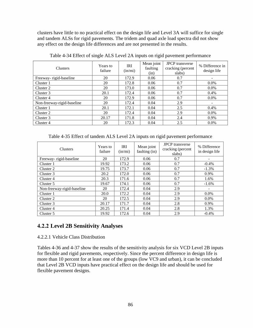
86
clusters have little to no practical effect on the design life and Level 3A will suffice for single
and tandem ALSs for rigid pavements. The tridem and quad axle load spectra did not show
any effect on the design life differences and are not presented in the results.
Table 4-34 Effect of single ALS Level 2A inputs on rigid pavement performance
Clusters Years to
failure
IRI
(in/mi)
Mean joint
faulting
(in)
JPCP transverse
cracking (percent
slabs)
% Difference in
design life
Freeway- rigid-baseline 20 172.9 0.06 0.7 -
Cluster 1 20 172.8 0.06 0.7 0.0%
Cluster 2 20 173.0 0.06 0.7 0.0%
Cluster 3 20.1 172.4 0.06 0.7 0.4%
Cluster 4 20 172.9 0.06 0.7 0.0%
Non-freeway-rigid-baseline 20 172.4 0.04 2.9 -
Cluster 1 20.1 172.1 0.04 2.5 0.4%
Cluster 2 20 172.4 0.04 2.9 0.0%
Cluster 3 20.17 171.8 0.04 2.4 0.9%
Cluster 4 20 172.3 0.04 2.5 0.0%
Table 4-35 Effect of tandem ALS Level 2A inputs on rigid pavement performance
Clusters Years to
failure
IRI
(in/mi)
Mean joint
faulting (in)
JPCP transverse
cracking (percent
slabs)
% Difference
in design life
Freeway- rigid-baseline 20 172.9 0.06 0.7 -
Cluster 1 19.92 173.2 0.06 0.7 -0.4%
Cluster 2 19.75 173.7 0.06 0.7 -1.3%
Cluster 3 20.2 172.0 0.06 0.7 0.9%
Cluster 4 20.3 171.6 0.06 0.7 1.6%
Cluster 5 19.67 174.1 0.06 0.7 -1.6%
Non-freeway-rigid-baseline 20 172.4 0.04 2.9 -
Cluster 1 20.0 172.2 0.04 2.9 0.0%
Cluster 2 20 172.5 0.04 2.9 0.0%
Cluster 3 20.17 171.7 0.04 2.8 0.9%
Cluster 4 20.25 171.4 0.04 2.8 1.3%
Cluster 5 19.92 172.6 0.04 2.9 -0.4%
4.2.2 Level 2B Sensitivity Analyses
4.2.2.1 Vehicle Class Distribution
Tables 4-36 and 4-37 show the results of the sensitivity analysis for six VCD Level 2B inputs
for flexible and rigid pavements, respectively. Since the percent difference in design life is
more than 10 percent for at least one of the groups (low VC9 and urban), it can be concluded
that Level 2B VCD inputs have practical effect on the design life and should be used for
flexible pavement designs.
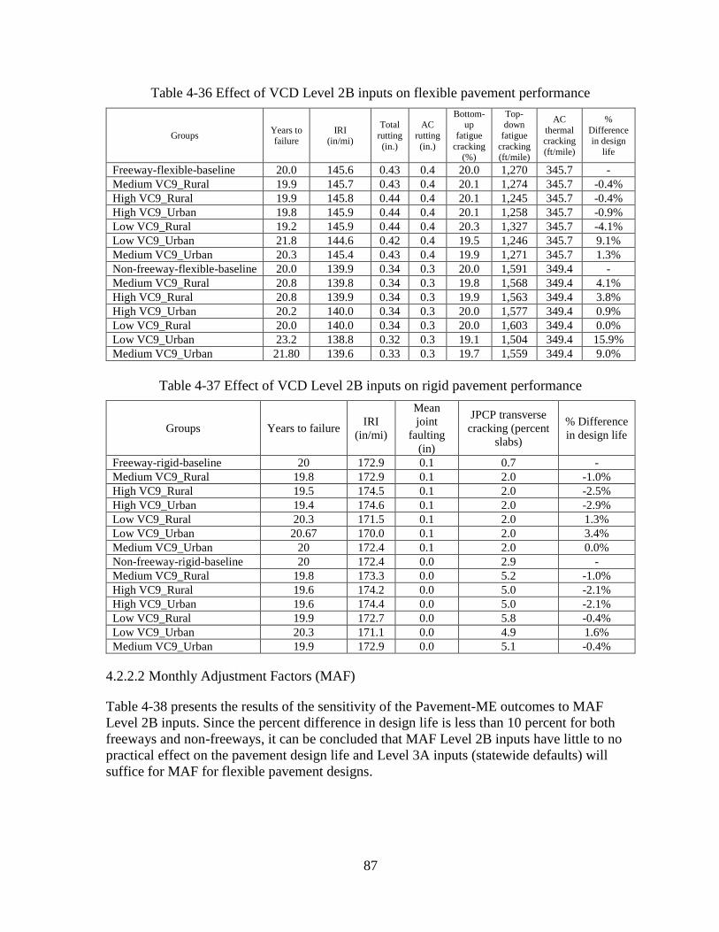
87
Table 4-36 Effect of VCD Level 2B inputs on flexible pavement performance
Groups Years to failure
IRI (in/mi)
Total
rutting
(in.)
AC
rutting
(in.)
Bottom-up
fatigue
cracking (%)
Top-down
fatigue
cracking (ft/mile)
AC
thermal cracking
(ft/mile)
%
Difference in design
life
Freeway-flexible-baseline 20.0 145.6 0.43 0.4 20.0 1,270 345.7 -
Medium VC9_Rural 19.9 145.7 0.43 0.4 20.1 1,274 345.7 -0.4%
High VC9_Rural 19.9 145.8 0.44 0.4 20.1 1,245 345.7 -0.4%
High VC9_Urban 19.8 145.9 0.44 0.4 20.1 1,258 345.7 -0.9%
Low VC9_Rural 19.2 145.9 0.44 0.4 20.3 1,327 345.7 -4.1%
Low VC9_Urban 21.8 144.6 0.42 0.4 19.5 1,246 345.7 9.1%
Medium VC9_Urban 20.3 145.4 0.43 0.4 19.9 1,271 345.7 1.3%
Non-freeway-flexible-baseline 20.0 139.9 0.34 0.3 20.0 1,591 349.4 -
Medium VC9_Rural 20.8 139.8 0.34 0.3 19.8 1,568 349.4 4.1%
High VC9_Rural 20.8 139.9 0.34 0.3 19.9 1,563 349.4 3.8%
High VC9_Urban 20.2 140.0 0.34 0.3 20.0 1,577 349.4 0.9%
Low VC9_Rural 20.0 140.0 0.34 0.3 20.0 1,603 349.4 0.0%
Low VC9_Urban 23.2 138.8 0.32 0.3 19.1 1,504 349.4 15.9%
Medium VC9_Urban 21.80 139.6 0.33 0.3 19.7 1,559 349.4 9.0%
Table 4-37 Effect of VCD Level 2B inputs on rigid pavement performance
Groups Years to failure IRI
(in/mi)
Mean
joint
faulting
(in)
JPCP transverse
cracking (percent
slabs)
% Difference
in design life
Freeway-rigid-baseline 20 172.9 0.1 0.7 -
Medium VC9_Rural 19.8 172.9 0.1 2.0 -1.0%
High VC9_Rural 19.5 174.5 0.1 2.0 -2.5%
High VC9_Urban 19.4 174.6 0.1 2.0 -2.9%
Low VC9_Rural 20.3 171.5 0.1 2.0 1.3%
Low VC9_Urban 20.67 170.0 0.1 2.0 3.4%
Medium VC9_Urban 20 172.4 0.1 2.0 0.0%
Non-freeway-rigid-baseline 20 172.4 0.0 2.9 -
Medium VC9_Rural 19.8 173.3 0.0 5.2 -1.0%
High VC9_Rural 19.6 174.2 0.0 5.0 -2.1%
High VC9_Urban 19.6 174.4 0.0 5.0 -2.1%
Low VC9_Rural 19.9 172.7 0.0 5.8 -0.4%
Low VC9_Urban 20.3 171.1 0.0 4.9 1.6%
Medium VC9_Urban 19.9 172.9 0.0 5.1 -0.4%
4.2.2.2 Monthly Adjustment Factors (MAF)
Table 4-38 presents the results of the sensitivity of the Pavement-ME outcomes to MAF
Level 2B inputs. Since the percent difference in design life is less than 10 percent for both
freeways and non-freeways, it can be concluded that MAF Level 2B inputs have little to no
practical effect on the pavement design life and Level 3A inputs (statewide defaults) will
suffice for MAF for flexible pavement designs.
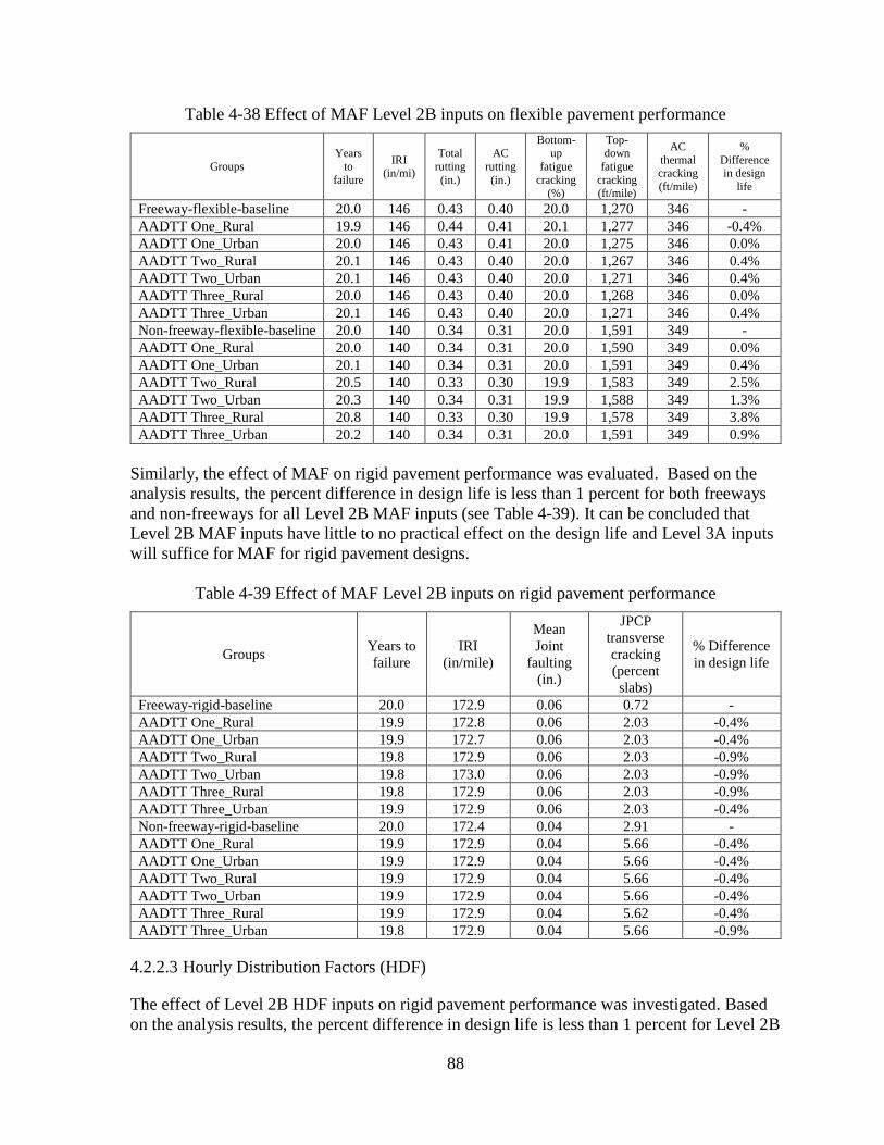
88
Table 4-38 Effect of MAF Level 2B inputs on flexible pavement performance
Groups
Years
to
failure
IRI (in/mi)
Total
rutting
(in.)
AC
rutting
(in.)
Bottom-up
fatigue
cracking (%)
Top-down
fatigue
cracking (ft/mile)
AC
thermal cracking
(ft/mile)
%
Difference in design
life
Freeway-flexible-baseline 20.0 146 0.43 0.40 20.0 1,270 346 -
AADTT One_Rural 19.9 146 0.44 0.41 20.1 1,277 346 -0.4%
AADTT One_Urban 20.0 146 0.43 0.41 20.0 1,275 346 0.0%
AADTT Two_Rural 20.1 146 0.43 0.40 20.0 1,267 346 0.4%
AADTT Two_Urban 20.1 146 0.43 0.40 20.0 1,271 346 0.4%
AADTT Three_Rural 20.0 146 0.43 0.40 20.0 1,268 346 0.0%
AADTT Three_Urban 20.1 146 0.43 0.40 20.0 1,271 346 0.4%
Non-freeway-flexible-baseline 20.0 140 0.34 0.31 20.0 1,591 349 -
AADTT One_Rural 20.0 140 0.34 0.31 20.0 1,590 349 0.0%
AADTT One_Urban 20.1 140 0.34 0.31 20.0 1,591 349 0.4%
AADTT Two_Rural 20.5 140 0.33 0.30 19.9 1,583 349 2.5%
AADTT Two_Urban 20.3 140 0.34 0.31 19.9 1,588 349 1.3%
AADTT Three_Rural 20.8 140 0.33 0.30 19.9 1,578 349 3.8%
AADTT Three_Urban 20.2 140 0.34 0.31 20.0 1,591 349 0.9%
Similarly, the effect of MAF on rigid pavement performance was evaluated. Based on the
analysis results, the percent difference in design life is less than 1 percent for both freeways
and non-freeways for all Level 2B MAF inputs (see Table 4-39). It can be concluded that
Level 2B MAF inputs have little to no practical effect on the design life and Level 3A inputs
will suffice for MAF for rigid pavement designs.
Table 4-39 Effect of MAF Level 2B inputs on rigid pavement performance
Groups Years to
failure
IRI
(in/mile)
Mean
Joint
faulting
(in.)
JPCP
transverse
cracking
(percent
slabs)
% Difference
in design life
Freeway-rigid-baseline 20.0 172.9 0.06 0.72 -
AADTT One_Rural 19.9 172.8 0.06 2.03 -0.4%
AADTT One_Urban 19.9 172.7 0.06 2.03 -0.4%
AADTT Two_Rural 19.8 172.9 0.06 2.03 -0.9%
AADTT Two_Urban 19.8 173.0 0.06 2.03 -0.9%
AADTT Three_Rural 19.8 172.9 0.06 2.03 -0.9%
AADTT Three_Urban 19.9 172.9 0.06 2.03 -0.4%
Non-freeway-rigid-baseline 20.0 172.4 0.04 2.91 -
AADTT One_Rural 19.9 172.9 0.04 5.66 -0.4%
AADTT One_Urban 19.9 172.9 0.04 5.66 -0.4%
AADTT Two_Rural 19.9 172.9 0.04 5.66 -0.4%
AADTT Two_Urban 19.9 172.9 0.04 5.66 -0.4%
AADTT Three_Rural 19.9 172.9 0.04 5.62 -0.4%
AADTT Three_Urban 19.8 172.9 0.04 5.66 -0.9%
4.2.2.3 Hourly Distribution Factors (HDF)
The effect of Level 2B HDF inputs on rigid pavement performance was investigated. Based
on the analysis results, the percent difference in design life is less than 1 percent for Level 2B
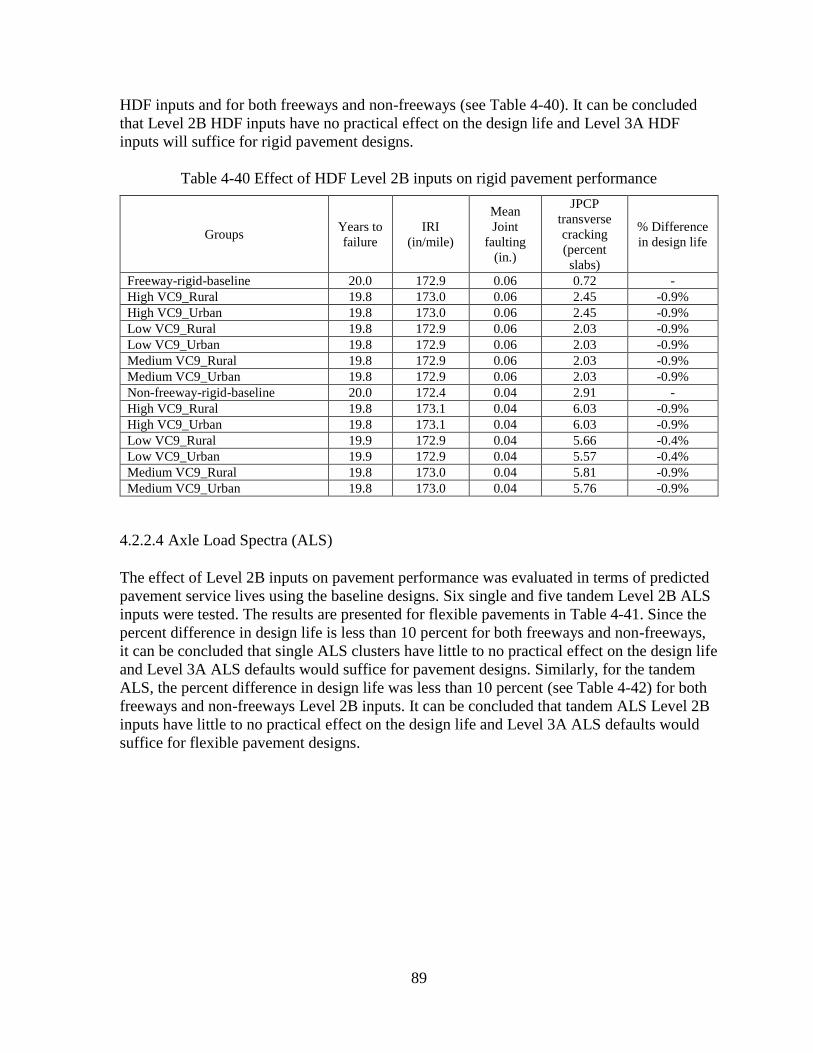
89
HDF inputs and for both freeways and non-freeways (see Table 4-40). It can be concluded
that Level 2B HDF inputs have no practical effect on the design life and Level 3A HDF
inputs will suffice for rigid pavement designs.
Table 4-40 Effect of HDF Level 2B inputs on rigid pavement performance
Groups Years to
failure
IRI
(in/mile)
Mean
Joint
faulting
(in.)
JPCP
transverse
cracking
(percent
slabs)
% Difference
in design life
Freeway-rigid-baseline 20.0 172.9 0.06 0.72 -
High VC9_Rural 19.8 173.0 0.06 2.45 -0.9%
High VC9_Urban 19.8 173.0 0.06 2.45 -0.9%
Low VC9_Rural 19.8 172.9 0.06 2.03 -0.9%
Low VC9_Urban 19.8 172.9 0.06 2.03 -0.9%
Medium VC9_Rural 19.8 172.9 0.06 2.03 -0.9%
Medium VC9_Urban 19.8 172.9 0.06 2.03 -0.9%
Non-freeway-rigid-baseline 20.0 172.4 0.04 2.91 -
High VC9_Rural 19.8 173.1 0.04 6.03 -0.9%
High VC9_Urban 19.8 173.1 0.04 6.03 -0.9%
Low VC9_Rural 19.9 172.9 0.04 5.66 -0.4%
Low VC9_Urban 19.9 172.9 0.04 5.57 -0.4%
Medium VC9_Rural 19.8 173.0 0.04 5.81 -0.9%
Medium VC9_Urban 19.8 173.0 0.04 5.76 -0.9%
4.2.2.4 Axle Load Spectra (ALS)
The effect of Level 2B inputs on pavement performance was evaluated in terms of predicted
pavement service lives using the baseline designs. Six single and five tandem Level 2B ALS
inputs were tested. The results are presented for flexible pavements in Table 4-41. Since the
percent difference in design life is less than 10 percent for both freeways and non-freeways,
it can be concluded that single ALS clusters have little to no practical effect on the design life
and Level 3A ALS defaults would suffice for pavement designs. Similarly, for the tandem
ALS, the percent difference in design life was less than 10 percent (see Table 4-42) for both
freeways and non-freeways Level 2B inputs. It can be concluded that tandem ALS Level 2B
inputs have little to no practical effect on the design life and Level 3A ALS defaults would
suffice for flexible pavement designs.
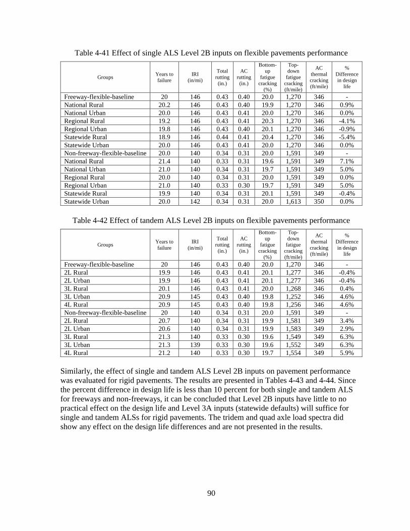
90
Table 4-41 Effect of single ALS Level 2B inputs on flexible pavements performance
Groups Years to failure
IRI (in/mi)
Total
rutting
(in.)
AC
rutting
(in.)
Bottom-up
fatigue
cracking (%)
Top-down
fatigue
cracking (ft/mile)
AC
thermal cracking
(ft/mile)
%
Difference in design
life
Freeway-flexible-baseline 20 146 0.43 0.40 20.0 1,270 346 -
National Rural 20.2 146 0.43 0.40 19.9 1,270 346 0.9%
National Urban 20.0 146 0.43 0.41 20.0 1,270 346 0.0%
Regional Rural 19.2 146 0.43 0.41 20.3 1,270 346 -4.1%
Regional Urban 19.8 146 0.43 0.40 20.1 1,270 346 -0.9%
Statewide Rural 18.9 146 0.44 0.41 20.4 1,270 346 -5.4%
Statewide Urban 20.0 146 0.43 0.41 20.0 1,270 346 0.0%
Non-freeway-flexible-baseline 20.0 140 0.34 0.31 20.0 1,591 349 -
National Rural 21.4 140 0.33 0.31 19.6 1,591 349 7.1%
National Urban 21.0 140 0.34 0.31 19.7 1,591 349 5.0%
Regional Rural 20.0 140 0.34 0.31 20.0 1,591 349 0.0%
Regional Urban 21.0 140 0.33 0.30 19.7 1,591 349 5.0%
Statewide Rural 19.9 140 0.34 0.31 20.1 1,591 349 -0.4%
Statewide Urban 20.0 142 0.34 0.31 20.0 1,613 350 0.0%
Table 4-42 Effect of tandem ALS Level 2B inputs on flexible pavements performance
Groups Years to
failure
IRI
(in/mi)
Total rutting
(in.)
AC rutting
(in.)
Bottom-
up fatigue
cracking
(%)
Top-
down fatigue
cracking
(ft/mile)
AC
thermal
cracking (ft/mile)
%
Difference
in design life
Freeway-flexible-baseline 20 146 0.43 0.40 20.0 1,270 346 -
2L Rural 19.9 146 0.43 0.41 20.1 1,277 346 -0.4%
2L Urban 19.9 146 0.43 0.41 20.1 1,277 346 -0.4%
3L Rural 20.1 146 0.43 0.41 20.0 1,268 346 0.4%
3L Urban 20.9 145 0.43 0.40 19.8 1,252 346 4.6%
4L Rural 20.9 145 0.43 0.40 19.8 1,256 346 4.6%
Non-freeway-flexible-baseline 20 140 0.34 0.31 20.0 1,591 349 -
2L Rural 20.7 140 0.34 0.31 19.9 1,581 349 3.4%
2L Urban 20.6 140 0.34 0.31 19.9 1,583 349 2.9%
3L Rural 21.3 140 0.33 0.30 19.6 1,549 349 6.3%
3L Urban 21.3 139 0.33 0.30 19.6 1,552 349 6.3%
4L Rural 21.2 140 0.33 0.30 19.7 1,554 349 5.9%
Similarly, the effect of single and tandem ALS Level 2B inputs on pavement performance
was evaluated for rigid pavements. The results are presented in Tables 4-43 and 4-44. Since
the percent difference in design life is less than 10 percent for both single and tandem ALS
for freeways and non-freeways, it can be concluded that Level 2B inputs have little to no
practical effect on the design life and Level 3A inputs (statewide defaults) will suffice for
single and tandem ALSs for rigid pavements. The tridem and quad axle load spectra did
show any effect on the design life differences and are not presented in the results.
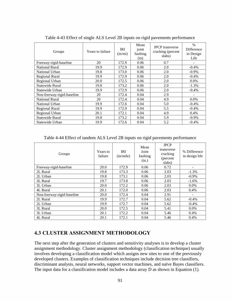
91
Table 4-43 Effect of single ALS Level 2B inputs on rigid pavements performance
Groups Years to failure IRI
(in/mi)
Mean
joint
faulting
(in)
JPCP transverse
cracking (percent
slabs)
%
Difference
in Design
Life
Freeway-rigid-baseline 20 172.9 0.06 0.7 -
National Rural 19.9 172.9 0.06 2.0 -0.4%
National Urban 19.8 173.0 0.06 2.0 -0.9%
Regional Rural 19.9 172.9 0.06 2.0 -0.4%
Regional Urban 20.0 172.5 0.06 2.0 0.0%
Statewide Rural 19.8 173.2 0.06 2.0 -1.3%
Statewide Urban 19.9 172.9 0.06 2.0 -0.4%
Non-freeway-rigid-baseline 20 172.4 0.04 2.9 -
National Rural 20 172.4 0.04 4.9 0.0%
National Urban 19.9 172.6 0.04 5.0 -0.4%
Regional Rural 19.9 172.9 0.04 5.5 -0.4%
Regional Urban 20.1 172.1 0.04 4.9 0.4%
Statewide Rural 19.8 173.2 0.04 5.9 -0.9%
Statewide Urban 19.9 172.6 0.04 5.2 -0.4%
Table 4-44 Effect of tandem ALS Level 2B inputs on rigid pavements performance
Groups Years to
failure
IRI
(in/mile)
Mean
Joint
faulting
(in.)
JPCP
transverse
cracking
(percent
slabs)
% Difference
in design life
Freeway-rigid-baseline 20.0 172.9 0.06 0.72 -
2L Rural 19.8 173.3 0.06 2.03 -1.3%
2L Urban 19.8 173.1 0.06 2.03 -0.9%
3L Rural 19.7 173.8 0.06 2.03 -1.6%
3L Urban 20.0 172.2 0.06 2.03 0.0%
4L Rural 20.1 172.0 0.06 2.03 0.4%
Non-freeway-rigid-baseline 20.0 172.4 0.04 2.91 -
2L Rural 19.9 172.7 0.04 5.62 -0.4%
2L Urban 19.9 172.7 0.04 5.62 -0.4%
3L Rural 20.0 172.5 0.04 5.41 0.0%
3L Urban 20.1 172.2 0.04 5.46 0.4%
4L Rural 20.1 172.1 0.04 5.46 0.4%
4.3 CLUSTER ASSIGNMENT METHODOLOGY
The next step after the generation of clusters and sensitivity analyses is to develop a cluster
assignment methodology. Cluster assignment methodology (classification technique) usually
involves developing a classification model which assigns new sites to one of the previously
developed clusters. Examples of classification techniques include decision tree classifiers,
discriminant analysis, neural networks, support vector machines, and naïve Bayes classifiers.
The input data for a classification model includes a data array D as shown in Equation (1).

92
Each row contains a data object, and the columns contain the attribute values and the class
label of each data object.
11 1 1
1
n
m mn m
x x y
D
x x y
(1)
where:
ijx = value of the jth attribute of object i.
iy = Class label of the object i
The attribute values (e.g., road class and development type) could be either discrete or
continuous while the class label (clusters) should always be discrete. All the classification
techniques use a learning algorithm to identify a model that best fits the relationship between
the attribute set and the class label of the input data. For this study, the attribute set includes
various attributes of the PTR locations. The class labels are the pre-defined cluster numbers.
The models generated by the learning algorithms should fit the input data well and correctly
predict the clusters of a new PTR location it has never seen before. The general approach in
developing a model is to have a training set of PTR locations whose cluster numbers are
known. This training set is used to develop a classification model. This model is then applied
to test set which consists of PTR locations and their clusters numbers not used by the model.
Evaluation of any classification model is based on its accurate number predictions of the
cluster numbers and can be presented in a tabular form called the confusion matrix (see Table
4-45).
Table 4-45 Confusion matrix for dataset with two class labels (clusters)
Confusion matrix Predicted Class
Cluster = 1 Cluster = 2
Actual
class
Cluster = 1 P11 P12
Cluster = 2 P21 P22
Each element in the diagonal (bolded) are predicted accurately and the non-diagonal
elements are the inaccurate predictions. One could use a performance metric of a model such
as accuracy as defined below.
11 22
11 12 21 22
Number of accurate predictionsAccuracy =
Total number of predictions
P P
P P P P
(2)
Consequently, the error rate is
12 21
11 12 21 22
Number of inaccurate predictionsError rate =
Total number of predictions
P P
P P P P
(3)

93
The error rate of a classification model can be divide into two categories (a) training error,
and (b) testing error. The training error is the misclassification rate of the model on the
training records. The testing error is the misclassification rate of the model using the data
which it has not seen before. A good classification model should have high accuracy and
low error rate.
As previously mentioned, several techniques exist for building a classification model but the
research team decided to use the decision tree classifiers for its ease of use. An example of a
decision tree can be seen in Figure 4-12. A decision tree has three types of nodes: (a) a root
node that has no incoming edges and zero or more outgoing edges (Development type) (b)
internal nodes, which have exactly one incoming edge and two or more outgoing edges
(Functional Class), and (c) leaf or terminal nodes, which has exactly on incoming edge and
no outgoing edges. Each leaf node is assigned the cluster number. Many decision trees can be
constructed from a given set of attributes. While some of the trees are more accurate than
others, finding the optimal tree is computationally infeasible. Many algorithms can be used to
decide on the attribute to be used for partitioning the data but the one most commonly used is
the Hunt’s algorithm which is the basis of many existing decision tree induction algorithms
(4).
Development Type
Functional Class Functional Class
Urban Rural
Freeway
Cluster 5
Non-
Freeway
Number of Lanes
Two Three
Cluster 1 Cluster 3
Freeway
Cluster 2
Non-
Freeway
COHS
National Regional
Cluster 4 Cluster 3
Figure 4-12 Example of a decision tree
The advantages of decision trees are that they are easy to understand and interpret. They can
handle both numerical and categorical data input data and can be used to solve problems with
multi-class labels (as opposed to certain techniques that can handle only binary class labels).
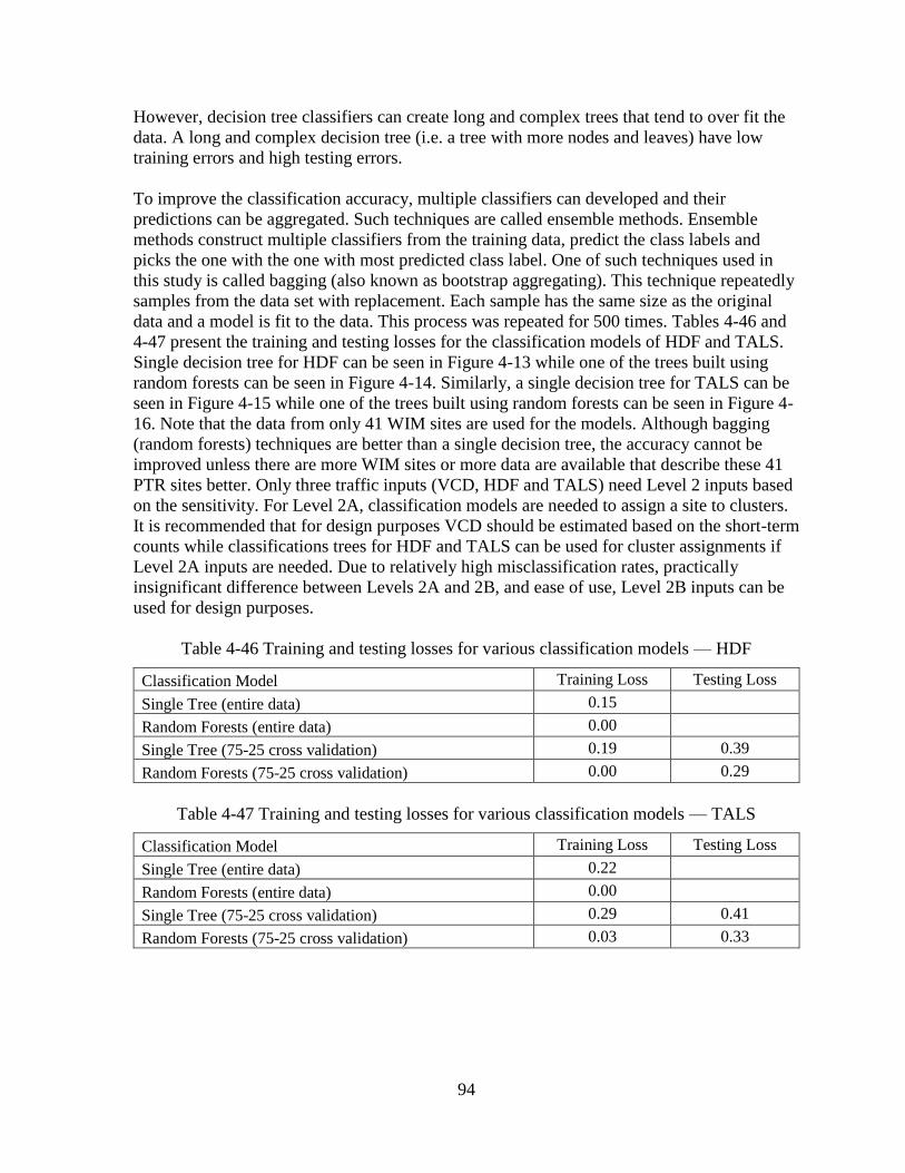
94
However, decision tree classifiers can create long and complex trees that tend to over fit the
data. A long and complex decision tree (i.e. a tree with more nodes and leaves) have low
training errors and high testing errors.
To improve the classification accuracy, multiple classifiers can developed and their
predictions can be aggregated. Such techniques are called ensemble methods. Ensemble
methods construct multiple classifiers from the training data, predict the class labels and
picks the one with the one with most predicted class label. One of such techniques used in
this study is called bagging (also known as bootstrap aggregating). This technique repeatedly
samples from the data set with replacement. Each sample has the same size as the original
data and a model is fit to the data. This process was repeated for 500 times. Tables 4-46 and
4-47 present the training and testing losses for the classification models of HDF and TALS.
Single decision tree for HDF can be seen in Figure 4-13 while one of the trees built using
random forests can be seen in Figure 4-14. Similarly, a single decision tree for TALS can be
seen in Figure 4-15 while one of the trees built using random forests can be seen in Figure 4-
16. Note that the data from only 41 WIM sites are used for the models. Although bagging
(random forests) techniques are better than a single decision tree, the accuracy cannot be
improved unless there are more WIM sites or more data are available that describe these 41
PTR sites better. Only three traffic inputs (VCD, HDF and TALS) need Level 2 inputs based
on the sensitivity. For Level 2A, classification models are needed to assign a site to clusters.
It is recommended that for design purposes VCD should be estimated based on the short-term
counts while classifications trees for HDF and TALS can be used for cluster assignments if
Level 2A inputs are needed. Due to relatively high misclassification rates, practically
insignificant difference between Levels 2A and 2B, and ease of use, Level 2B inputs can be
used for design purposes.
Table 4-46 Training and testing losses for various classification models — HDF
Classification Model Training Loss Testing Loss
Single Tree (entire data) 0.15
Random Forests (entire data) 0.00
Single Tree (75-25 cross validation) 0.19 0.39
Random Forests (75-25 cross validation) 0.00 0.29
Table 4-47 Training and testing losses for various classification models — TALS
Classification Model Training Loss Testing Loss
Single Tree (entire data) 0.22
Random Forests (entire data) 0.00
Single Tree (75-25 cross validation) 0.29 0.41
Random Forests (75-25 cross validation) 0.03 0.33
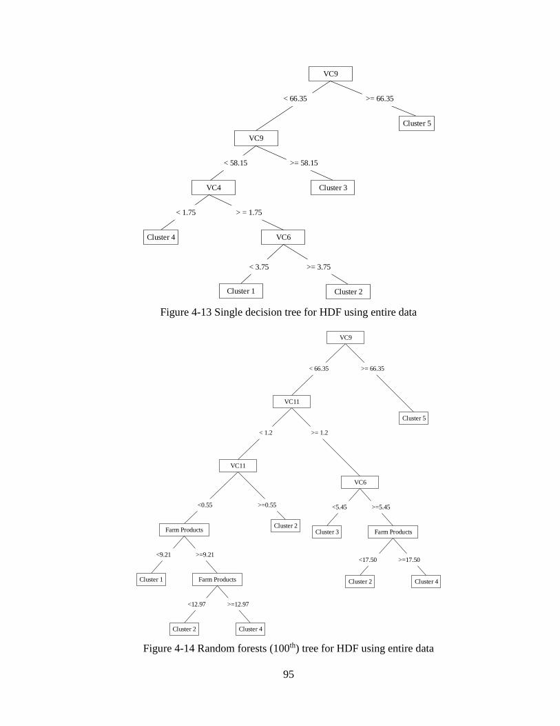
95
Figure 4-13 Single decision tree for HDF using entire data
Figure 4-14 Random forests (100th) tree for HDF using entire data
VC9
VC9
Cluster 5
< 66.35 >= 66.35
< 58.15
VC4
>= 58.15
VC6
< 3.75 >= 3.75
Cluster 1 Cluster 2
Cluster 3
< 1.75
Cluster 4
> = 1.75
Farm Products
<0.55
<9.21
Cluster 1
>=9.21
Farm Products
<12.97 >=12.97
Cluster 2 Cluster 4
<5.45
Cluster 3
>=5.45
Cluster 2 Cluster 4
>=0.55
Cluster 2
VC9
Cluster 5
VC11
< 66.35 >= 66.35
VC11
< 1.2 >= 1.2
VC6
Farm Products
<17.50 >=17.50
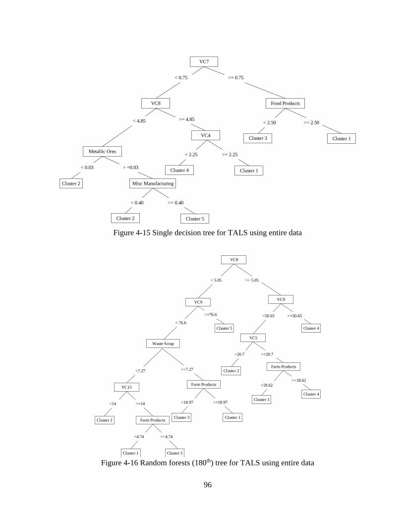
96
Figure 4-15 Single decision tree for TALS using entire data
Figure 4-16 Random forests (180th) tree for TALS using entire data
VC7
VC8
< 0.75 >= 0.75
< 4.85 >= 4.85
< 0.40 >= 0.40
Cluster 2 Cluster 5
VC4
< 0.03
Cluster 2
> =0.03
< 2.50 >= 2.50
Cluster 3 Cluster 1
< 2.25 >= 2.25
Cluster 4 Cluster 1
Food Products
Metallic Ores
Misc Manufacturing
<7.27
<14
Cluster 2
>=14
Farm Products
<4.74 >=4.74
Cluster 1 Cluster 5
<20.7
Cluster 2
>=20.7
Cluster 3
Cluster 4
>=7.27
VC8
VC9
< 5.05 >= 5.05
< 76.6
>=76.6
VC5
Farm Products
<18.62>=18.62
<18.97 >=18.97
Cluster 3 Cluster 1
<50.65
Cluster 5
VC9
>=50.65
Cluster 4
Waste Scrap
Farm ProductsVC13

97
4.4 SUMMARY
Five traffic input levels were developed in this study as listed below.
a. Level 1 – Site-specific inputs
b. Level 2A – Averages of clusters based on cluster analyses
c. Level 2B – Averages of groups based on roadway characteristics (attributes)
d. Level 3A – Averages based on freeway and non-freeway road classes
e. Level 3B – Statewide averages
Level 1 inputs should always be used for design purposes wherever possible as it is the actual
traffic data specific to the site. When Level 1 traffic inputs are unavailable, either Levels 2 or
3 inputs have to be used for pavement designs. The impact of Level 2 inputs on predicted
pavement performance can be evaluated by using sensitivity analyses. If no differences in the
predicted performance or pavement lives are observed between Levels 1 and 2 inputs, Level
3 traffic inputs will suffice for pavement design. The steps involved in sensitivity analyses
include establishing base designs, performance criteria and other input parameters in the
Pavement-ME and then evaluating the impact of Levels 2 and 3 traffic inputs.
For sensitivity analyses, the pavement design life was assumed 20 years with 95% design
reliability for flexible and rigid pavements. For each of the 41 WIM locations, the HMA
surface layer thickness was designed to achieve a 20-year design life for bottom-up fatigue
cracking threshold of 20% for flexible pavements since it is a critical structural distress for
pavement design. Level 1 inputs were used in this process. For these designs, the rut depth
values at the end of 20 years were also recorded. In addition, for each of the 41 WIM
locations, the slab thickness was designed to achieve a 20-year design life for IRI threshold
of 172 inches/mile for the rigid pavements because it controls most of the designs. Faulting
and transverse cracking values were also recorded at the end of 20 years. For both the
flexible and rigid pavement designs, one traffic input was changed at a time to Levels 2A and
2B to determine their effects on the design lives. Levels 3A and 3B inputs for each design
(one input at a time) were also used in the Pavement-ME to determine their impact on the
design lives. The time for the distress values (for Levels 2 and 3) to reach the threshold
values in the Level 1 designs were documented. The differences in design lives between
different inputs levels were quantified for further analyses.
Statistical analyses could detect differences between clusters or groups, but the differences
might not have much practical significance. Hence, in addition to the statistical significance,
the maximum life difference (MLD) values between two input levels were adopted as an
indicator of the variability in the data and correspondingly select the proper input level
needed for the design. One way ANOVA was performed on the absolute life differences
(|LifeLevel 1 - LifeLevel X|) to detect the differences between the clusters for each traffic input. If
the p-value is below 0.05, the results indicate that the cluster or group averages are different
from each other and that their use in pavement design would result in statistically different
design lives. However, it does not indicate whether the differences are of practical
significance. The absolute differences in predicted lives were estimated relative to Level 1
design life of 20 years. The cluster or group was considered sensitive or of practical

98
significance if the absolute life differences of at least one WIM location is higher than two
years.
Once the sensitivity of inputs at Levels 2 and 3 was determined, the next step was to identify
if there are any differences between predicted lives for Levels 2A and 2B. If there are no
differences between the Levels 2A and 2B, then Level 2B can be used since it will simplify
the input selection process. A paired t-test was used to verify if there are significant
differences between the values of (|LifeLevel 1 - LifeLevel 2A |) and (|LifeLevel 1 - LifeLevel 2B|).
Also, the number of under- and over-designed WIM sites due to the use of Levels 2A and 2B
inputs were determined. A pavement at a WIM location will be overdesigned when the
difference in design lives (LifeLevel 1 - LifeLevel x) is positive and under-designed when the
difference (LifeLevel 1 - LifeLevel x) is negative. While a positive life difference would suggest
increasing the thicknesses making the project over-designed, a negative life difference will
force to reduce the thicknesses making the project under-designed relative to Level 1. If there
were statistically significant differences, either Level 2A or 2B was selected for that traffic
input after careful evaluation of the average design life differences. If there were no
differences between Levels 2A and 2B, comparisons were made between Levels 2A and 3A
or 2B and 3A to see if Level 3A would suffice for pavement designs. Again, if there are no
differences between Levels 2 and 3A, comparisons were made between Levels 3A and 3B to
see if Level 3B would suffice for pavement designs. Subsequent to the sensitivity analyses,
classifications models (decision trees) were developed for cluster assignment.
The criteria used in this analyses to establish significant traffic inputs are based on
engineering judgment and local experience. The statistical analyses may not be reliable
alone; practical significance should always support it. Based on the sensitivity analyses of
Levels 2A, 2B, 3A, and 3B, it is recommended that for design purposes VCD should be
estimated based on the short-term counts while classifications trees for HDF and TALS can
be used for cluster assignments if Level 2A inputs are needed. Due to relatively high
misclassification rates, practically insignificant difference between Levels 2A and 2B, and
ease of use, Level 2B inputs can be used for design purposes. The following input levels are
recommended for each traffic input (see Table 4-48).
Table 4-48 Recommended traffic input levels
Traffic input Recommended traffic input level
Flexible pavements Rigid pavements
VCD 2B 2B
HDF - 2B
MAF 3A 3A
SALS 3A 3A
TALS 2B 2B
TRALS 3A 3A
QALS 3A 3A
99
CHAPTER 5 - PREPME EVALUATION
5.1 BACKGROUND
The Pavement-ME design (previously MEPDG/DARWin-ME) is a substantial advancement
in pavement design process. Therefore, it requires many more inputs from various data
sources. Through the transportation pooled fund study TPF-5(242): Traffic and Data
Preparation for AASHTO Pavement-ME Analysis and Design, a full-production software
called PrepME with comprehensive database features was developed to assist state DOTs in
data preparation and improve the management and workflow of the Pavement-ME design
input data. Specifically, the PrepME is capable of pre-processing, importing, checking the
quality of raw Weigh-In-Motion (WIM) traffic data, and generating three traffic input levels
with in-built clustering analysis methods. This tool can be used not only by pavement design
engineers to prepare input for the Pavement-ME, but also traffic data collection engineers to
collect better traffic data and manage those data for other applications. The software has the
following basic functions with more specific features requested by individual States.
Imports an agency’s PTR traffic data complying with FHWA Traffic Monitoring
Guide (TMG) file formats, and stores the data in SQL server local database with
exceptional computation efficiency.
Conducts Travel Monitoring Analysis System (TMAS 2.0) data check during data
import and generates TMAS check error log for each imported raw file.
Performs automatic quality control checks by direction and lane for both
classification and weight data based on the TMG recommendations.
Provides user friendly interfaces to review monthly, weekly and daily traffic data, and
investigate the PTR data that is incomplete or fails the automatic QC check through
various manual, sampling, and analyzing operations.
Generates three levels of traffic inputs: Level 1 site specific, Level 2 clustering
average, Level 3 state average, LTPP TPF-5(004), and the Pavement-ME defaults.
Offers clustering methods developed by North Carolina and Michigan DOTs,
Kentucky Transportation Cabinet (KYTC), Truck Traffic Classification (TTC)
method, simplified TTC approach, and flexible clustering for generating Level 2
loading spectra inputs for the Pavement-ME based on the availability of traffic data.
Generates input files in the file formats that can be directly imported into the
Pavement-ME software.
5.2 UPDATES IN PREPME
Several major functional improvements have been made in the updated PrepME software,
including:
100
5.2.1 Traffic Data Import Module
The updated PrepME has the capability to automatically check and determine the data
format of WIM data, and import WIM data following both the 2001 and 2013 TMG
formats into the PrepME SQL database.
A new function has been developed to merge multiple classification (CLA) or Weight
(WGT) files into a single file. Due to the characteristic of PrepME data flow, the
speed of importing a single combined CLA or WGT file is much faster than that of
multiple files separately. Users can find this new feature in the Tool menu.
Besides the detailed TMAS check report developed in the past, a summary TMAS
quick check report is also generated during data import process. The summary TMAS
report could help state agencies diagnose the sensor issues.
5.2.2 Traffic Data Check Module
New functions are added to display data for multiple user-selected months. This
feature is helpful to investigate the traffic patterns for WIM stations on low volume
roads.
Several error prevention operations are added in the process of "Run Quality Control"
in the Classification Data Check Module to prevent software crashes for some
specific stations which have no data.
A function that is able to cancel users’ manual operation
Two changes have been made for the "Monthly Sampling" operation to allow the data
to be classified as "accepted" after a monthly sampling operation was performed.
The team re-examined the data flow of the "Daily Sampling" operation. The updated
PrepME software now only allows users to select complete weekly data to represent
the traffic data for the month.
5.2.3 Traffic Data Output
A function is developed to automatically compute several key traffic parameters for a
selected PTR site, including AADTT, Trucks% in Designed Direction, Trucks% in
Designed Lane. This function can compute AADTT in either both directions or one
direction for Level 1 site-specific output. In addition, the updated PrepME can
automatically determine design direction & design lane for such calculations.
All traffic output files generated by PrepME are re-validated with Pavement ME
Design, since the XML data format for Pavement ME Design has been changed.
In addition, several software bugs have been fixed including:
Previously PrepME crashes when users try to enter the traffic output dialog if either
CLA or WGT data are available. This bug has been fixed in the most recent software.
Due to Google Map API changes, the previous version of PrepME software
encounters a script error and crashes when the Google Map capability is called by the
software. The software has been updated using the most recent Google Map API. In
addition, if no GPS information is available for a specific PTR site, the Google Map

101
will mark this site in the middle of the Pacific Ocean. In the updated PrepME, if such
information is missing, the location is pointed to the center of the state.
After clicking the button "Show WIM Station" in STA Data Check Module, software
will crash if there is no CLA and WGT data. New codes were added to (1) prevent
software from crashing under this condition; (2) merge repeatable information in a
STA file during the importing process;
In the "View Output Data" in the Traffic Output Module, the logical order among the
radio buttons is corrected.
It is found that the output axle loading spectra in the previous version of the PrepME
software were shifted by one load bin to the heavier side for all the four axle types.
This bug has been fixed in the PrepME import module.
5.3 PREPME QC DATA CHECKS
The Traffic Data Check sub-menu is able to:
Conduct QC check for weight data by direction and lane of traffic using data check
algorithms defined in the TMG (Figure 5-1). Weight data check algorithms defined in
the 2001 third edition of TMG are integrated in the PrepME software to evaluate
weight data for class 9 vehicles. Specific weight bounds can be defined for the front
axle and drive tandem axle weights of Class 9 trucks. In addition, the histogram plot
of gross vehicle weights of Class 9 trucks should have two peaks, one representing
unloaded Class 9 trucks between 28,000 and 36,000 lb (32,000 ± 4,000 lb), and the
second peak representing loaded vehicle condition with a weigh between 72,000 and
80,000 lb (76,000 ± 4,000 lb).
Provide interfaces for users to review monthly, weekly, and daily traffic data.
Provide four sampling and repair options to analyze and utilize incomplete (that not
have a minimum of 12-month data) or failed data (that cannot pass the automatic
TMG data check algorithms), including Manual Operation (Accept and Reject),
Replacement (Copy and Paste), and Sampling Operation (Daily Sampling and
Monthly Sampling).
o Manual Operation (Accept/Reject) allows users to review and double check
the automated QC results.
o Replacement (Copy and Paste) operation can be used to check the similarity
of the data in adjacent months, opposite direction, or different lane, same
month but different year, and then identify a suitable month which can be used
as the “source month” to substitute the failed or missing month (the “target
month”).
o Daily Sampling operation can be used as a diagnostic tool to investigate the
reason(s) for bad data that cannot pass automatic data check, and sample
weekly data with good quality to represent this month. (Figure 5-2)
o Monthly Sampling can be used to select twelve months of data with the
highest data quality, either right after a WIM system calibration or any 12
months' data based on engineering judgment.
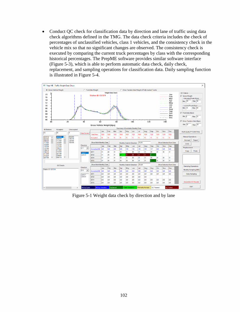
102
Conduct QC check for classification data by direction and lane of traffic using data
check algorithms defined in the TMG. The data check criteria includes the check of
percentages of unclassified vehicles, class 1 vehicles, and the consistency check in the
vehicle mix so that no significant changes are observed. The consistency check is
executed by comparing the current truck percentages by class with the corresponding
historical percentages. The PrepME software provides similar software interface
(Figure 5-3), which is able to perform automatic data check, daily check,
replacement, and sampling operations for classification data. Daily sampling function
is illustrated in Figure 5-4.
Figure 5-1 Weight data check by direction and by lane
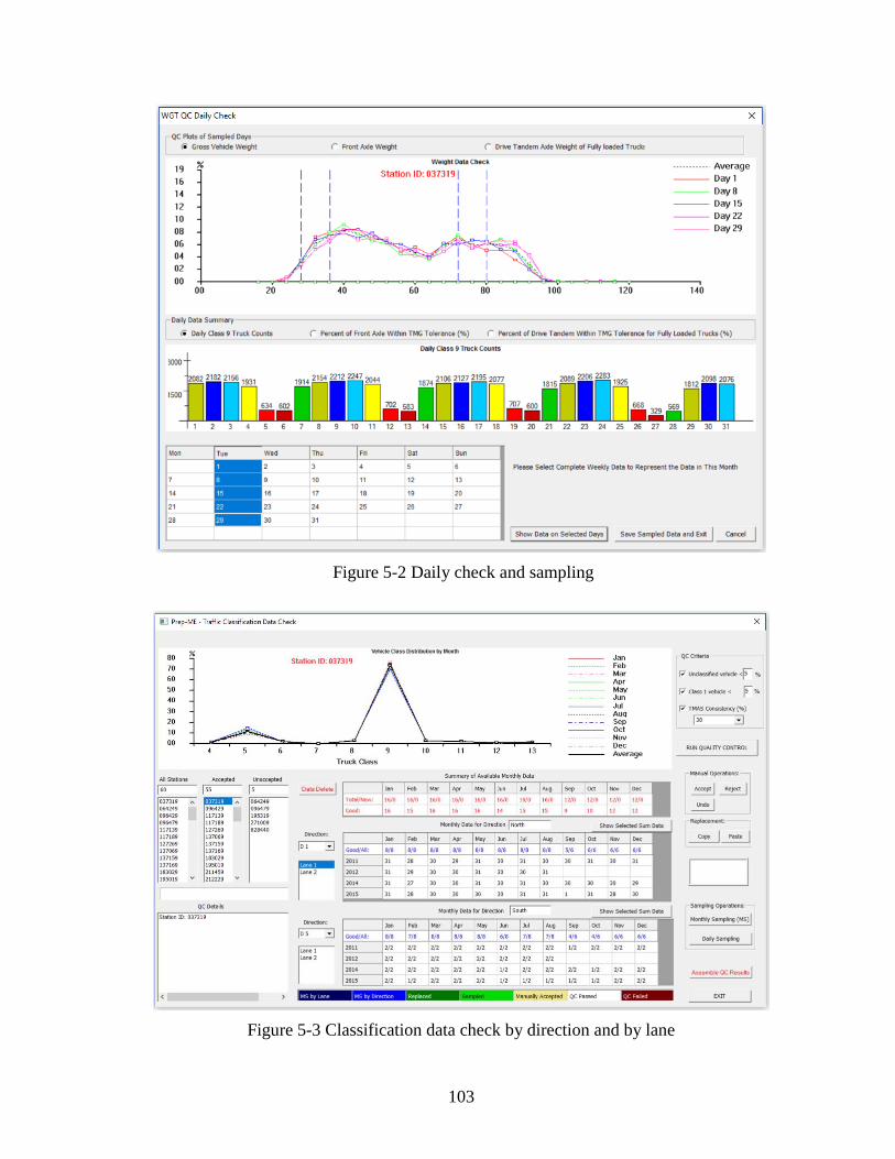
103
Figure 5-2 Daily check and sampling
Figure 5-3 Classification data check by direction and by lane
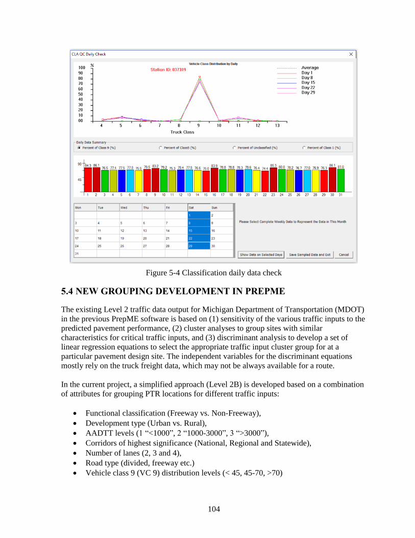
104
Figure 5-4 Classification daily data check
5.4 NEW GROUPING DEVELOPMENT IN PREPME
The existing Level 2 traffic data output for Michigan Department of Transportation (MDOT)
in the previous PrepME software is based on (1) sensitivity of the various traffic inputs to the
predicted pavement performance, (2) cluster analyses to group sites with similar
characteristics for critical traffic inputs, and (3) discriminant analysis to develop a set of
linear regression equations to select the appropriate traffic input cluster group for at a
particular pavement design site. The independent variables for the discriminant equations
mostly rely on the truck freight data, which may not be always available for a route.
In the current project, a simplified approach (Level 2B) is developed based on a combination
of attributes for grouping PTR locations for different traffic inputs:
Functional classification (Freeway vs. Non-Freeway),
Development type (Urban vs. Rural),
AADTT levels (1 “<1000”, 2 “1000-3000”, 3 “>3000”),
Corridors of highest significance (National, Regional and Statewide),
Number of lanes (2, 3 and 4),
Road type (divided, freeway etc.)
Vehicle class 9 (VC 9) distribution levels (< 45, 45-70, >70)

105
The possible 2-, 3-, and 4-way combinations of the attributes are investigated in the project.
Pairwise Euclidean distances between each sublevel combinations are calculated to identify
the combination of the attributes that show different traffic patterns. Due to the extensive
computing complexity required in the process, the optimal combination of the attributes has
not been fully integrated in the software programming. Instead, only 2-way combination
results are implemented in the updated PrepME software. Note that the traffic loading spectra
output data are averaged based on the selected WIM sites. In addition, the attributes used in
the site selection process are hardcoded in the software. The users cannot implement addition
of new sites and attribute modifications in the software currently.
Figure 5-5 shows the new software interface. Users should select any two attributes (out of
the seven) to generate output averages for various traffic parameters. The steps to export
desired traffic inputs for the Pavement-ME design are as follows:
1. Traffic data preparation: Follow the Prep-ME User’s Guide to import traffic data and
perform necessary quality checks.
2. Export traffic data setup: Provide the “Project Name” and the directory for data output
using the “Export Data To…” button. The GPS coordinates are optional, which are only
used for the Google Map utility. Subsequently, the “MIDOT Method 2” should be
selected to use the simplified Level 2B approach. In the popped-up attribute selection
window, users can select two of the attributes for their design. If a different combination
is desired, the “Reset Selection” button can clear the previous selection of attributes so
that new combinations can be selected.
3. Export traffic data for Pavement ME Design: Click the “OK” button after the attribute
combination is set and the traffic data is ready for review and export.
Figure 5-5 New developed Level 2B two-way combination grouping approach
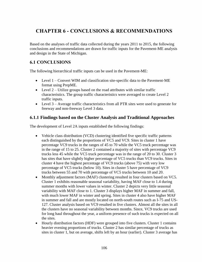
106
CHAPTER 6 - CONCLUSIONS & RECOMMENDATIONS
Based on the analyses of traffic data collected during the years 2011 to 2015, the following
conclusions and recommendations are drawn for traffic inputs for the Pavement-ME analysis
and design in the State of Michigan.
6.1 CONCLUSIONS
The following hierarchical traffic inputs can be used in the Pavement-ME:
Level 1 – Convert WIM and classification site-specific data to the Pavement-ME
format using PrepME.
Level 2 – Utilize groups based on the road attributes with similar traffic
characteristics. The group traffic characteristics were averaged to create Level 2
traffic inputs.
Level 3 – Average traffic characteristics from all PTR sites were used to generate for
freeway and non-freeway Level 3 data.
6.1.1 Findings based on the Cluster Analysis and Traditional Approaches
The development of Level 2A inputs established the following findings:
Vehicle class distribution (VCD) clustering identified five specific traffic patterns
each distinguished by the proportions of VC5 and VC9. Sites in cluster 1 have
percentage VC9 trucks in the ranges of 45 to 70 while the VC5 truck percentage was
in the range of 15 to 25. Cluster 2 contained a majority of sites with percentage VC9
trucks less 45 while the VC5 truck percentage was in the range of 20 to 30. Cluster 3
has sites that have slightly higher percentage of VC5 trucks than VC9 trucks. Sites in
cluster 4 have the highest percentage of VC9 trucks (above 75) with very low
percentage of VC5 trucks (below 10). Sites in cluster 5 have percentage of VC9
trucks between 55 and 70 with percentage of VC5 trucks between 10 and 20.
Monthly adjustment factors (MAF) clustering resulted in four clusters based on VC5.
Cluster 1 exhibits reasonable seasonal variability, having MAF close to 1.4 during
summer months with lower values in winter. Cluster 2 depicts very little seasonal
variability with MAF close to 1. Cluster 3 displays higher MAF in summer and fall,
with much lower MAF in winter and spring. Sites in cluster 4 also have higher MAF
in summer and fall and are mostly located on north-south routes such as I-75 and US-
127. Cluster analysis based on VC9 resulted in five clusters. Almost all the sites in all
the clusters have no seasonal variability between months. Since, VC9 trucks are used
for long haul throughout the year, a uniform presence of such trucks is expected on all
the sites.
Hourly distribution factors (HDF) were grouped into five clusters. Cluster 1 contains
heavier evening proportions of trucks. Cluster 2 has similar percentage of trucks as
sites in cluster 1, but on average, shifts left by an hour (earlier). Cluster 3 average has
107
roughly a 1-2% lower truck percentage between the hours of 7:00 am and 4:00 pm
than either clusters 1 or 2. Sites in cluster 4 have the highest HDF during 8 am to 12
noon of all clusters. Sites in cluster 5 have the flattest curve among all the clusters
suggesting minimum hourly variations for long-haul trucks.
Single axle load spectra (SALS) were grouped into four clusters based on VC5 trucks.
For all the sites in the clusters the first peak occurs at approximately 4 to 6 kips while
the second peak occurs at 8 to 10 kips. Cluster 1 has almost equal proportion of axles
in the 4-6 kip range and the 8-10 kip range. Cluster 2 has higher proportion of 4-6 kip
axles than 8-10 kip axles. Cluster 3 has only one site (US-2) in the Upper Peninsula
and the pattern is unique to that site. Cluster 4 has sites with higher proportion of
axles in the 8-10 kip range than the 4-6 kip range.
Tandem axle load spectra (TALS) based on VC9 resulted in five clusters. The two
peaks in the clusters correspond to unloaded (9-14 kips) and loaded (30-33 kips)
trucks. Clusters 1, 3 and 4 have more light axles than heavy, whereas Clusters 2 and
Cluster 5 have heavier tandem axles.
Tridem axle load spectra (TRALS) based on VC13 formed six clusters. The general
trend of the tridem axle clusters show a large proportion of light axles around 12 kips
followed by a peak value around 40-45 kips.
Quad axle load spectra (QALS) based on VC13 resulted in 3 clusters. Peak values for
the quad axle load spectra occur at the 18-24 kips, 45-60 kip ranges.
The development of Level 2B inputs established the following findings:
It was anticipated that the MDOT will know the AADTT at a site (i.e., from historical
traffic data or short-term counts). Therefore, AADTT was grouped into low, medium,
and high traffic volume. Low was under 1000 AADTT, medium was from 1000 to
3000 AADTT, and high was greater than 3000 AADTT for the design lane in one
direction. Fourteen sites had low AADTT, eighteen sites had medium AADTT, and
the remaining nine had high AADTT. Note that the AADTT brackets were
determined based on the distribution of the latest AADTT levels from the 41 PTR
sites.
For VCD, the attributes of VCD level and development type (urban vs. rural) resulted
in six groups. Three distinct patterns with varying levels of VC9 irrespective of the
development type were observed. All the sites in high VC9 groups are located on the
interstates while most of the sites in low VC9 groups are located on state routes. Sites
in the medium VC9 groups have a mix of both intestates and state routes in rural and
urban areas.
For MAF, the attributes of commercial AADT and development type resulted in six
groups. Almost all the groups have similar MAF patterns for VC5 except for sites
with low AADTT in the rural areas suggesting seasonal traffic patterns. No
differences in MAF for VC9 trucks were found between the groups and are always
close to 1.
For HDF, the attributes of VCD level and development type resulted in six groups.
The sites having low VC9 levels in the urban areas have the highest peak among all
other groups between 8:00 am and 4:00 pm suggesting local traffic patterns. Sites
having high VC9 levels have the flattest peaks in both urban and rural areas

108
suggesting long haul traffic patterns. All the sites in high VC9 groups are on
interstate routes.
For SALS, the attributes of COHS and development type resulted in six groups. For
all the sites in different groups, the first peak occurs at approximately 4-6 kips while
the second peak occurs at 8-10 kips. Road groups in the urban areas have almost
equal proportion of axles in the 4-6 kip range and the 8-10 kip range while the sites in
the rural areas have higher proportion of 4-6 kip axles than 8-10 kip axles. The road
group of regional corridor in the urban area has only one site on US-2 with a unique
loading pattern.
For TALS, the attributes of number of lanes and development type resulted in five
groups. The two peaks seem to correspond to unloaded (9-14 kips) and loaded (30-33
kips) tandem axles. Other characteristics could not be established for the groups as
they have varying functional classifications and AADTT levels and also due to the
fact that some groups only have one site.
For TRALS, the attributes of COHS and development type resulted in six groups. The
general trend of the tridem axle groups appears to be a large proportion of light axles
around 12 kips followed by a peak value around 40-45 kips. All the sites in the
national corridors are located on interstates while the sites on regional and statewide
corridors are on state routes with varying AADTT levels irrespective of the
development type.
For QALS, the attributes of COHS and development type resulted in six groups.
Again, all the sites in national corridors are on the interstates while the sites on
regional and statewide corridors are on state routes with varying AADTT levels
irrespective of the development type.
6.1.2 Significant Traffic Input Levels
For pavement design, it is recommended that site specific data (Level 1) be used if available.
For sites with no site-specific data, it is necessary to know whether Level 2 or Level 3 data
are acceptable for design purposes. To investigate the impact of traffic input levels on
predicted pavement performance for flexible and rigid pavements, the Pavement-ME was
used. The results of the sensitivity analyses were used to establish the appropriate traffic
input levels. Such analyses were performed on the absolute life differences (|LifeLevel 1 -
LifeLevel X|) to detect the differences between the clusters or groups for each traffic input.
The sensitivity of inputs at Levels 2 and 3 was determined using statistical and practical
significance criteria. The next step was to identify if there are any differences between
predicted lives for Levels 2A and 2B. If there are no differences between the Levels 2A and
2B, then Level 2B can be used since it will simplify the input selection process. Also, the
number of under- and over-designed WIM sites due to the use Levels 2A and 2B inputs were
determined. A pavement at a location will be over-designed when the difference in design
lives (LifeLevel 1 - LifeLevel x) is positive and under-designed when the difference (LifeLevel 1 -
LifeLevel x) is negative. While a positive life difference would suggest increasing the
thicknesses making the project over-designed, a negative life difference will require to
reduce the thicknesses making the project under-designed relative to Level 1. If there were
statistically significant differences, either Level 2A or 2B was selected for that traffic input

109
after careful evaluation of the average design life differences. If there were no differences
between Levels 2A and 2B, comparisons were made between Levels 2A and 3A or 2B and
3A to see if Level 3A would suffice for pavement designs. Again, if there are no differences
between Levels 2 and 3A, comparisons were made between Levels 3A and 3B to see if Level
3B would suffice for pavement designs. Levels 2A, 2B, 3A and 3B traffic inputs can be
found in Appendix E. The following is the summary of findings:
VCD significantly impacts predicted rigid and flexible pavement performance. In
addition there is a statistical difference between Levels 2A and 2B for rutting only in
flexible pavements. The number of under designed sites are higher for Level 2A
compared to Level 2B. Thus, VCD groups (Level 2B) are suggested for use in
flexible and rigid pavement design.
MAF have negligible impact on predicted rigid and flexible pavement performance.
No statistical differences in design lives between Level 2A clusters or 2B road groups
were observed. Also, there are no statistically significant differences between Levels
2B and 3A. Since there are statistically significant differences between Levels 3A and
3B, Level 3A inputs are recommended for MAF for both flexible and rigid pavements
HDF significantly impacts rigid pavement performance. Level 2A is slightly better
with the number of undersigned sites for transverse cracking than Level 2B.
However, due to relatively high misclassification rates of the classification models,
practically insignificant difference between Levels 2A and 2B, and ease of use, group
average (Level 2B) HDFs should be utilized for rigid pavement design.
AGPV had a negligible impact on predicted rigid and flexible pavement performance.
Therefore, it is suggested that statewide averages (Level 3B) be used for this traffic
input.
Single axle load spectra have a significant effect on predicted flexible pavement
performance. Cluster (2A) and group (2B) averages produced comparable results.
Also no significant difference was detected between Levels 2B and 3A. Therefore, it
is recommended that statewide averages (Level 3A) be used for this traffic input.
Tandem axle load significantly impacted rigid and flexible pavement performance.
Therefore, group averages (Level 2B) are suggested for both rigid and flexible
pavement designs.
Tridem and quad axle load spectra do not have a significant impact on rigid and
flexible pavement performance. Consequently, statewide average tridem and quad
axle load spectra (Level 3A) can be used for this traffic input.
The Pavement-ME defaults traffic inputs don’t accurately reflect the local traffic
conditions in the state of Michigan. In general, statewide or cluster averages produced
performance lives that were closer to the site-specific values than the Pavement-ME
defaults. Consequently, the Pavement-ME defaults are not recommended for use in
the state of Michigan.
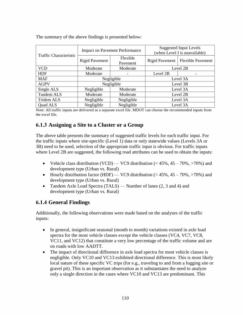
110
The summary of the above findings is presented below:
Traffic Characteristic
Impact on Pavement Performance Suggested Input Levels
(when Level I is unavailable)
Rigid Pavement Flexible
Pavement Rigid Pavement Flexible Pavement
VCD Moderate Moderate Level 2B
HDF Moderate - Level 2B -
MAF Negligible Level 3A
AGPV Negligible Level 3B
Single ALS Negligible Moderate Level 3A
Tandem ALS Moderate Moderate Level 2B
Tridem ALS Negligible Negligible Level 3A
Quad ALS Negligible Negligible Level 3A Note: All traffic inputs are delivered as a separate excel file. MDOT can choose the recommended inputs from
the excel file.
6.1.3 Assigning a Site to a Cluster or a Group
The above table presents the summary of suggested traffic levels for each traffic input. For
the traffic inputs where site-specific (Level 1) data or only statewide values (Levels 3A or
3B) need to be used, selection of the appropriate traffic input is obvious. For traffic inputs
where Level 2B are suggested, the following road attributes can be used to obtain the inputs:
Vehicle class distribution (VCD) — VC9 distribution (< 45%, 45 – 70%, >70%) and
development type (Urban vs. Rural)
Hourly distribution factor (HDF) — VC9 distribution (< 45%, 45 – 70%, >70%) and
development type (Urban vs. Rural)
Tandem Axle Load Spectra (TALS) — Number of lanes (2, 3 and 4) and
development type (Urban vs. Rural)
6.1.4 General Findings
Additionally, the following observations were made based on the analyses of the traffic
inputs:
In general, insignificant seasonal (month to month) variations existed in axle load
spectra for the most vehicle classes except the vehicle classes (VC4, VC7, VC8,
VC11, and VC12) that constitute a very low percentage of the traffic volume and are
on roads with low AADTT.
The impact of directional difference in axle load spectra for most vehicle classes is
negligible. Only VC10 and VC13 exhibited directional difference. This is most likely
local nature of these specific VC trips (for e.g., traveling to and from a logging site or
gravel pit). This is an important observation as it substantiates the need to analyze
only a single direction in the cases where VC10 and VC13 are predominant. This

111
difference should be observed for each PTR location where directional difference for
VC13 is more than 5%.
The single axle load distribution depends on the percentages of VC5 and VC9 in the
traffic stream. The sites with higher proportions of VC5 peak at 4-8 kips while sites
with higher proportions VC9 peak at 8-10 kips.
The tandem axle load distributions are mostly dependent on the axle load spectra of
VC9.
The tridem and quad axle load spectra are a function of VC7, VC10 and VC13.
6.2 RECOMMENDATIONS
It is recommended, wherever possible, to expand the geographic coverage of traffic data in
Michigan. When a new PTR site needs to be installed, it should be located in areas where
limited traffic data are available. Short duration and continuous counts should be shared
between agencies to ensure wider and recurrent data collection coverage. Effective
communication between traffic data collection personnel and pavement design engineers is
recommended for addressing the traffic input requirement for the Pavement-ME.
Additionally, the following specific traffic data collection efforts should be considered as
recommended by the Traffic Monitoring Guide (TMG):
The short duration volume coverage count program should provide comprehensive
coverage across the roadway infrastructure on a cycle of 6 years. Short duration
classification counts should account for at least 25-30% of all volume counts being
conducted (i.e., at all PTR locations) wherever possible. In addition, at least one
vehicle classification count should be made on each route annually.
At least six continuous vehicle classification PTR be established for each road group.
Continuous counts should be placed on different functional classes and different
geographic regions within the state. Emphasis should be placed on roads that are
primarily local or long hauls. When new sites are added, the data should be placed
into the appropriate existing road groups.
A minimum of six WIM should be monitored within a group, with at least one of the
WIM sites operating continuously and recording two or more lanes of traffic. The
amount of permanent WIM stations and discontinuous portable systems is a function
of the number of groups, the accuracy at which the measured weights are taken, and
the budget of the State agency.
With proper coverage of existing groups and a gradual expansion into unmonitored areas
within the State through installation of permanent devices, the data collection program could
be more robust. In addition to above mentioned general suggestions, based on the results of
this study following are the specific recommendations to improve traffic data collection to
facilitate the use of the Pavement-ME design process in the State of Michigan:
1. The attributes selected for the road group development for different traffic inputs
were determined based on the traffic data collected at 41 WIM sites distributed across
the State. In addition, most of the traffic data were collected between years 2011 to
112
2015. However, there will be a need to revise these groups for Level 2B traffic inputs
if the following updates or changes are anticipated:
a. Addition of new classification and WIM sites at different geographical
locations or change in the status of existing site (e.g., down- or up-grading
from WIM to classification or vice versa).
b. Significant change in the land use (for e.g., industrial development or
commercial zoning) in the vicinity of the existing WIM locations.
c. Change in the WIM technology for a number of locations. For example if less
accurate piezo sensors are replaced with more accurate quartz or bending plate
sensors. The accuracy and bias in WIM sensor will affect the axle load spectra
which might influence the selection of attributes for Level 2B inputs.
If MDOT anticipates the above-mentioned updates or changes in the near future (e.g.,
5 or 10 years), then there will be a need to re-evaluate the attributes or the group
averages for all traffic inputs.
2. For a few sites, the traffic patterns over time were compared. Some changes in truck
traffic distribution were observed for PTR locations with one-way AADTT < 1000.
However, for sites having one-way AADTT > 1000, the truck traffic and tandem axle
distributions did not vary substantially for the last 5 years (2011 to 2015). If changes
are observed in traffic patterns (classifications and loadings) at a PTR location for at
least 3 years, then the new 3 years traffic data should be used to update the traffic
inputs. Otherwise, the new data should be combined with the available traffic
database. These changes in traffic patterns include any of the following at a PTR
location:
a. A 10% change in VC9 and VC10,
b. An 8% change in VC11, and
c. A 5% change in VC13
3. The existing PTR locations were reviewed and the following specific WIM additions
are recommended for the various regions in the State:
a. Superior Region:
Because of the presence of heavy to very heavy axle loads, an additional
WIM site along M28 between Ewen and Kenton.
To capture interstate truck traffic (between Michigan and Wisconsin), an
addition WIM site should be considered on US2 west of Watersmeet.
b. North Region:
The current WIM site distribution seems adequate with the addition of
WIM site 3069 to cover the west side of the region.
An additional WIM sites should be considered on the eastern side along
M-32 if land use demands change in future.
c. Grand Region:

113
The axle loading analysis revealed light to medium axle loadings in this
region. Therefore, the current WIM site distribution seems adequate at this
time.
d. Bay Region:
This region also contains light to medium axle loadings. The current WIM
site distribution seems adequate at this time.
e. Metro Region:
Additional WIM can be considered on I-75 between Flint and Auburn
Hills. No PTR is located on this part of I-75 with anticipated commercial
truck traffic.
f. University Region:
Based on the new axle loading data, the current WIM site distribution
seems adequate at this time.
g. Southwest Region:
Additional WIM site is recommended in future on US31 near Sodus
Township. This location will capture traffic coming north from I-90.
4. It is strongly recommended to continue collecting short-term (48 hours) counts to
obtain VCD data, especially for locations on interstate highways with higher
frequency of VC13. The VCD obtained using short-term count can be directly used in
the Pavement-ME as Level 1 input instead of Level 2B VCD input.
114
REFERENCES
Chapter 1
1. Zhang, Z., J. Leidy, I. Kawa, and W. Hudson, "Impact of changing traffic
characteristics and environmental conditions on flexible pavements," Transportation
Research Record: Journal of the Transportation Research Board, pp. 125-131, 2000.
2. Carvalho, R. and C. Schwartz, "Comparisons of flexible pavement designs: AASHTO
empirical versus NCHRP Project 1-37A mechanistic-empirical," Transportation
Research Record: Journal of the Transportation Research Board, pp. 167-174, 2006.
3. NCHRP, "Guide for Mechanistic-Empirical Design of New and Rehabilitated
Pavement Structures.," Washington D.C NCHRP Project 1-37A, 2004.
4. Buch, N., S. W. Haider, J. Brown, and K. Chatti, "Characterization of Truck Traffic
in Michigan for the New Mechanistic-Empirical Pavement Design Guide " Michigan
Department of Transportation, Lansing, MI Report # RC-1537, 2009.
5. NCHRP Project 1-37A, "Appendix AA: Traffic Loading," ARA, inc., ERES division,
505 West University Avenue, Champaign, Illinois 61820, 2004 Final Report: Guide
for Mechanistic-Empirical Design of New and Rehabilitated Pavement Structures,
2004.
6. Haider, S. W., N. Buch, K. Chatti, and J. Brown, "Development of Traffic Inputs for
Mechanistic-Empirical Pavement Design Guide in Michigan," Transportation
Research Record, vol. 2256, pp. 179-190, 2011.
7. FHWA, "Traffic Monitoring Guide," Washington, DC 2016.
8. Selezneva, O., M. Ayres, M. Hallenbeck, A. Ramachandran, H. Shirazi, and H. Von
Quintus, "MEPDG Traffic Loading Defaults Derived from LTPP Traffic Pooled Fund
Study," Federal Highway Administration, Final Report, FHWA, In the publication,
2016.
9. Selezneva, O. I., and M. Hallenbeck, "Long-Term Pavement Performance Pavement
Loading User Guide (LTPP PLUG)," Federal Highway Administration, FHWA-
HRT-13-089, 2013.
Chapter 2
1. NCHRP, "Guide for Mechanistic-Empirical Design of New and Rehabilitated
Pavement Structures.," Washington D.C NCHRP Project 1-37A, 2004.
2. Olga, S. and V. Q. Harold, "Traffic Load Spectra for Implementing and Using the
Mechanistic-Empirical Pavement Design Guide in Georgia," FHWA-GA-14-1009,
2014.
3. Tran, N. and K. Hall, "Development and significance of statewide volume adjustment
factors in mechanistic-empirical pavement design guide," Transportation Research
Record: Journal of the Transportation Research Board, pp. 97-105, 2007.
4. Lu, Q., Y. Zhang, and J. Harvey, "Estimation of truck traffic inputs for mechanistic-
empirical pavement design in California," Transportation Research Record: Journal
of the Transportation Research Board, pp. 62-72, 2009.
5. FHWA, "Traffic Monitoring Guide," Washington, DC 2016.

115
6. Lu, Q. and J. Harvey, "Characterization of truck traffic in California for mechanistic-
empirical design," Transportation Research Record: Journal of the Transportation
Research Board, pp. 61-72, 2006.
7. On Tam, W. and H. Von Quintus, "Use of long-term pavement performance data to
develop traffic defaults in support of mechanistic-empirical pavement design
procedures," Transportation Research Record: Journal of the Transportation
Research Board, pp. 176-182, 2003.
8. NCHRP Project 1-37A, "Appendix AA: Traffic Loading," ARA, inc., ERES division,
505 West University Avenue, Champaign, Illinois 61820, 2004 Final Report: Guide
for Mechanistic-Empirical Design of New and Rehabilitated Pavement Structures,
2004.
9. NCHRP, "NCHRP Report 538 : Traffic Data Collection, Analysis, and Forecasting
for Mechanistic Pavement Design," Transportation Research Board, Washington,
D.C. 2005.
10. Selezneva, O., M. Ayres, M. Hallenbeck, A. Ramachandran, H. Shirazi, and H. Von
Quintus, "MEPDG Traffic Loading Defaults Derived from LTPP Traffic Pooled Fund
Study," Federal Highway Administration, Final Report, FHWA, In publication, 2016.
11. Darter, M., L. Titus-Glover, and D. Wolf, "Development of a Traffic Data Input
System in Arizona for the MEPDG," Arizona Department of Transportation, Phoenix,
AZ FHWA-AZ-13-672, 2013.
12. Turochy, R. E., D. H. Timm, and D. Mai, "Development of Alabama Traffic Factors
for use in Mechanistic-Empirical Pavement Design," FHWA/ALDOT 930-793,
2015.
13. Buch, N., S. W. Haider, J. Brown, and K. Chatti, "Characterization of Truck Traffic
in Michigan for the New Mechanistic Empirical Pavement Design Guide " Michigan
Department of Transportation, Lansing, MI Report # RC-1537, 2009.
14. Wang, K. C., Q. Li, K. D. Hall, V. Nguyen, and D. X. Xiao, "Development of truck
loading groups for the mechanistic-empirical pavement design guide," Journal of
Transportation Engineering, vol. 137, pp. 855-862, 2011.
15. Agresti, A. and M. Kateri, Categorical data analysis: Springer, 2011.
16. Mallela, J., L. Titus-Glover, S. Sadasivam, B. Bhattacharya, M. Darter, and H. Von
Quintus, "Implementation of the AASHTO Mechanistic-empirical Pavement Design
Guide for Colorado," CDOT-2013-4, 2013.
17. Stone, J. R., Y. R. Kim, G. F. List, W. Rasdorf, F. Sayyady, F. Jadoun, and A. N.
Ramachandran, "Development of Traffic Data Input Resources for the Mechanistic
Empirical Pavement Design Process," FHWA/NC/2008-11, 2011.
18. Sayyady, F., J. Stone, G. List, F. Jadoun, Y. Kim, and S. Sajjadi, "Axle load
distribution for mechanistic-empirical pavement design in north carolina:
Multidimensional clustering approach and decision tree development,"
Transportation Research Record: Journal of the Transportation Research Board, pp.
159-168, 2011.
19. El-Badawy, S. M., F. M. Bayomy, and S. W. Fugit, "Traffic characteristics and their
impact on pavement performance for the implementation of the mechanistic-
empirical pavement design guide in Idaho," International Journal of Pavement
Research and Technology, vol. 5, pp. 386-394, 2012.

116
Chapter 3
1. Wang, K. C., Q. J. Li, V. Nguyen, M. Moravec, and D. Zhang, "Prep-ME: A multi-
agency effort to prepare data for DARWin-ME," in Airfield and Highway Pavement
2013: Sustainable and Efficient Pavements, 2013, pp. 516-527.
2. Turochy, R. E., D. H. Timm, and D. Mai, "Development of Alabama Traffic Factors
for use in Mechanistic-Empirical Pavement Design," FHWA/ALDOT 930-793,
2015.
3. FHWA, "Traffic Monitoring Guide," Washington, DC 2016.
4. Milligan, G. W., "Clustering Validation: Results and Implications for Applied
Analyses," in Clustering and Classification: World Scientific, 1996, pp. 341-375.
5. Tan, P. N., M. Steinbach, and V. Kumar, Introduction to Data Mining: Pearson, 2013.
6. Mooi, E. and M. Sarstedt, "Cluster analysis," in A Concise Guide to Market Research:
Springer, 2010, pp. 237-284.
7. Everitt, B. S., S. Landau, M. Leese, and D. Stahl, "Cluster analysis: Wiley series in
probability and statistics," Chichester: Wiley, 2011.
8. Baulieu, F., "A classification of presence/absence based dissimilarity coefficients,"
Journal of Classification, vol. 6, pp. 233-246, 1989.
9. Cheetham, A. H. and J. E. Hazel, "Binary (presence-absence) similarity coefficients,"
Journal of Paleontology, pp. 1130-1136, 1969.
10. Gower, J. C. and P. Legendre, "Metric and Euclidean properties of dissimilarity
coefficients," Journal of classification, vol. 3, pp. 5-48, 1986.
11. Hubalek, Z., "Coefficients of association and similarity, based on binary (presence‐
absence) data: an evaluation," Biological Reviews, vol. 57, pp. 669-689, 1982.
12. Yim, O. and K. T. Ramdeen, "Hierarchical cluster analysis: comparison of three
linkage measures and application to psychological data," Quant. Methods. Psychol,
vol. 11, pp. 8-21, 2015.
13. Steinbach, M., L. Ertöz, and V. Kumar, "The Challenges of Clustering High
Dimensional Data," in New directions in Statistical Physics: Springer, 2004, pp. 273-
309.
14. Ferreira, L. and D. B. Hitchcock, "A comparison of hierarchical methods for
clustering functional data," Communications in Statistics-Simulation and
Computation, vol. 38, pp. 1925-1949, 2009.
15. Milligan, G. W. and M. C. Cooper, "An examination of procedures for determining
the number of clusters in a data set," Psychometrika, vol. 50, pp. 159-179, 1985.
16. Caliński, T. and J. Harabasz, "A dendrite method for cluster analysis,"
Communications in Statistics-theory and Methods, vol. 3, pp. 1-27, 1974.
17. Matlab, 2016.
18. Tibshirani, R., G. Walther, and T. Hastie, "Estimating the number of clusters in a data
set via the gap statistic," Journal of the Royal Statistical Society: Series B (Statistical
Methodology), vol. 63, pp. 411-423, 2001.
19. Hallenbeck, M., M. Rice, B. Smith, C. Cornell-Martinez, and J. Wilkinson, "Vehicle
volume distributions by classification," 1997.
20. Schneider, W. H. and I. Tsapakis, "Review of Traffic Monitoring Factor Groupings
and the Determination of Seasonal Adjustment Factors for Cars and Trucks,"
University of Akron, Department of Civil Engineering 2009.

117
Chapter 4
1. Haider, S. W., G. Musunuru, M. E. Kutay, M. A. Lanotte, and N. Buch,
"Recalibration of Mechanistic-Empirical Rigid Pavement Performance Models and
Evaluation of Flexible Pavement Thermal Cracking Model," Report Number: SPR-
1668, 2017.
2. Haider, S. W., N. Buch, W. Brink, K. Chatti, and G. Baladi, "Preparation for
Implementation of the Mechanistic-Empirical Pavement Design Guide in Michigan
Part 3: Local Calibration and Validation of the Pavement-ME Performance Models,"
Rep. No. RC-1595, Michigan State Univ., East Lansing, MI, 2014.
3. Freund, R. J., W. J. Wilson, and D. L. Mohr, Statistical Methods, 3rd ed. London,
UK: Academic Press, An Imprint of Elsevier, 2010.
4. Tan, P. N., M. Steinbach, and V. Kumar, Introduction to Data Mining: Pearson, 2013.