University of Texas at Arlington Dissertation Template · Web viewThis is taken into account during the multiplexing process as explained in section 4.4. Table 5.1 gives the details

MULTIPLEXING H.264 VIDEO WITH AAC AUDIO BIT STREAMS,

DEMULTIPLEXING AND ACHIEVING LIP SYNCHRONIZATION

DURING PLAYBACK

by

HARISHANKAR MURUGAN

Presented to the Faculty of the Graduate School of

The University of Texas at Arlington in Partial Fulfillment

of the Requirements

for the Degree of

MASTER OF SCIENCE IN ELECTRICAL ENGINEERING

THE UNIVERSITY OF TEXAS AT ARLINGTON

May 2007

i

Copyright © by Harishankar Murugan 2007

All Rights Reserved

ii

ACKNOWLEDGEMENTS

I am grateful to my thesis advisor, Dr. K.R.Rao, for introducing me to video

coding and for his guidance and encouragement through out the thesis. He has been a

great source of inspiration and help in completing my thesis.

I would like to extend my sincere gratitude to UTA, for providing me the

opportunity and required resources to excel in my graduate studies.

I wish to thank Dr. T. Ogunfunmi and other lab members for their guidance and

suggestions on the implementation.

I would like to acknowledge Ahmad Hassan, staff engineer, streaming

networks, Islamabad, for his help in obtaining the utility to extract the test sequences.

I would like to express my appreciation to Dr. Z. Wang and Dr. A. Davis for

being a part of my thesis committee.

Finally, I would like to thank my parents and friends for their continuous

support in all my endeavors, without which this would not have been possible.

March 13, 2007

iii

ABSTRACT

MULTIPLEXING H.264 VIDEO WITH AAC AUDIO BIT STREAMS,

DEMULTIPLEXING AND ACHIEVING LIP SYNCHRONIZATION

DURING PLAYBACK

Publication No. ______

Harishankar Murugan , MS

The University of Texas at Arlington, 2007

Supervising Professor: Dr. K. R. Rao

H.264, MPEG-4 part-10 or AVC [5], is the latest digital video codec standard

which has proven to be superior than earlier standards in terms of compression ratio,

quality, bit rates and error resilience. However, the standard just defines a video codec

and has no mention of any audio compression. In order to have a meaningful delivery of

the video to the end user, it is necessary to associate an audio stream along with it. AAC

(advanced audio coding) [1] is the latest digital audio codec standard defined in MPEG-

2 and later in MPEG-4 with few changes. The audio quality of an AAC stream is

observed to be better than both MP3 and AC3, which were widely used as the audio

iv

coding standard in various applications, at lower bit rates. Adopting H.264 as video

codec and AAC as the audio codec, for transmission of digital multimedia through air

(ATSC, DVB) or through the internet (video streaming, IPTV), facilitates the users to

take advantage of the leading technologies in both audio and video. However, for these

applications, treatment of video and audio as separate streams requires multiplexing the

two in order to create a single bit stream for transmission. The objective of the thesis is

to propose a method for effectively multiplexing the audio and video coded streams for

transmission followed by demultiplexing the streams at the receving end and achieve lip

sync between the audio and video during playback. The proposed method takes

advantage of the frame wise arrangement of data in both audio and video codecs. The

audio and video frames are used as the first layer of packetization. The frame numbers

of the audio and video data blocks are used as the reference for aligning the streams in

order to achieve lip sync. The synchronizing information is embedded in the headers of

the first layer of packetization. Then second layer of packetization is carried out from

the first layer in order to meet the various requirements of transmission channels.

Proposed method uses playback time as the criteria for allocating data packets during

multiplexing in order to prevent buffer overflow or underflow at the demultiplexer end.

More information is embedded into the headers to ensure an effective and fast

demultiplexing process, to detect errors and correct them. Advantages and limitations of

the proposed method are discussed in detail.

v

TABLE OF CONTENTS

ACKNOWLEDGEMENTS....................................................................................... iii

ABSTRACT............................................................................................................... iv

LIST OF ILLUSTRATIONS..................................................................................... ix

LIST OF TABLES..................................................................................................... x

ACRONYMS AND ABBREVIATIONS ................................................................. xi

Chapter

1. INTRODUCTION ……..………………………………………………..... 1

1.1 Introduction …………............................................................................. 1

1.2 Thesis outline……………………………………………....................... 2

2. OVERVIEW OF H264 …............................................................................. 4

2.1 H.264/AVC………………...................................................................... 4

2.2 H.264/AVC profiles………………......................................................... 5

2.3 H.264/AVC encoder………………........................................................ 7

2.4 H.264 video decoder………………........................................................ 11

2.5 H.264 video bit stream………………..................................................... 12

2.6 Summary……………….......................................................................... 16

3. OVERVIEW OF AAC………………… ..................................................... 17

vi

3.1 Advanced audio coding…………………………………….................... 17

3.2 AAC profiles………………………………............................................ 18

3.3 AAC encoder…………………………………………........................... 19

3.4 Summary………………………………….............................................. 24

4. MULTIPLEXING…………………………………….................................. 25

4.1 Need for multiplexing………………………………………………….. 25

4.2 Factors to be considered for multiplexing and transmission…………… 26

4.3 Packetization………………………………………………………….... 27

4.3.1 Packetized elementary stream .................................................. 28

4.3.2 Transport stream....................................................................... 31

4.4 Frame number as timestamp.................................................................... 35

4.4.1 Advantages of frame numbers over clock samples as timestamps ......................................................................... 37

4.5 Proposed multiplexing method................................................................ 38

4.6 Summary…………………….................................................................. 39

5. DEMULTIPLEXING AND SYNCHRONIZATION…………................... 40

5.1 Demultiplexing…………………………………………………............ 40

5.2 Synchronization and playback……………………………...…………… 43

5.3 Summary…………………….................................................................. 45

6. RESULTS AND CONCLUSION.................................................................. 46

vii

6.1 Implementation and results...................................................................... 46

6.2 Conclusions…………………………...................................................... 49

6.3 Future research……………..................................................................... 49

REFERENCES.......................................................................................................... 50

BIOGRAPHICAL INFORMATION………………………………………………. 55

APPENDIX A: Multiplexing source code…………………………………………. 57

APPENDIX B: Demultiplexing source code…………..…………………………... 70

viii

LIST OF ILLUSTRATIONS

Figure Page

2.1 Profile structure in H.264................................................................................. 5

2.2 Block diagram of H.264 encoder..................................................................... 7

2.3 Mode decisions for intra prediction................................................................. 10

2.4 Block diagram of the decoder.......................................................................... 12

2.5 NAL unit syntax............................................................................................... 13

3.1 AAC encoder block diagram........................................................................... 19

4.1 Digital television transmission scheme............................................................ 26

4.2 Two layers of packetization............................................................................. 28

4.3 PES encapsulation from elementary stream.................................................... 29

4.4 TS packet formation from PES packet............................................................ 32

4.5 Calculation of playback time of a TS packet................................................... 39

5.1 Flowchart of the demultiplexer........................................................................ 40

ix

LIST OF TABLES

Table Page

2.1 Different NAL unit types................................................................................. 14

3.1 ADTS header format........................................................................................ 23

3.2 ADTS profile bits in header............................................................................. 24

4.1 PES packet header description......................................................................... 30

4.2 TS packet header description........................................................................... 33

5.1 Buffer fullness at demultiplexer using proposed method................................ 43

5.2 Buffer fullness at demultiplexer using alternative method.............................. 44

6.1 Results of multiplexed stream on test clip....................................................... 49

6.2 Observed synchronization delay on test clip................................................... 50

x

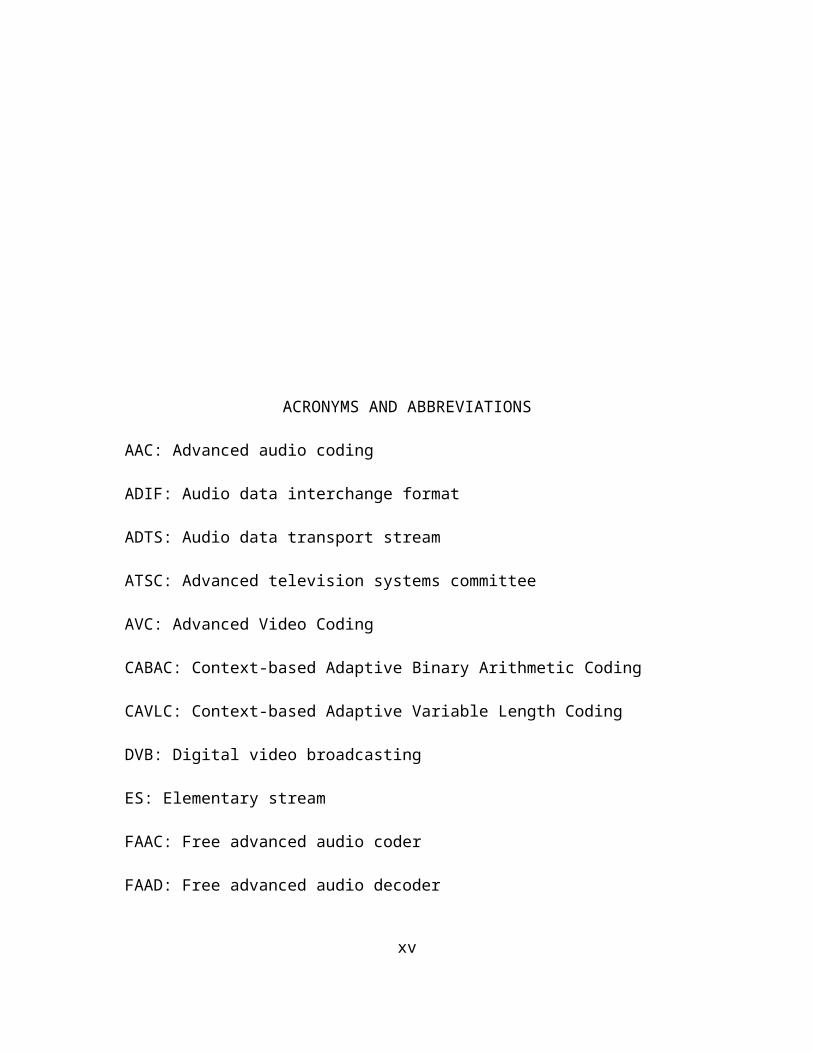
ACRONYMS AND ABBREVIATIONS

AAC: Advanced audio coding

ADIF: Audio data interchange format

ADTS: Audio data transport stream

ATSC: Advanced television systems committee

AVC: Advanced Video Coding

CABAC: Context-based Adaptive Binary Arithmetic Coding

CAVLC: Context-based Adaptive Variable Length Coding

DVB: Digital video broadcasting

ES: Elementary stream

FAAC: Free advanced audio coder

FAAD: Free advanced audio decoder

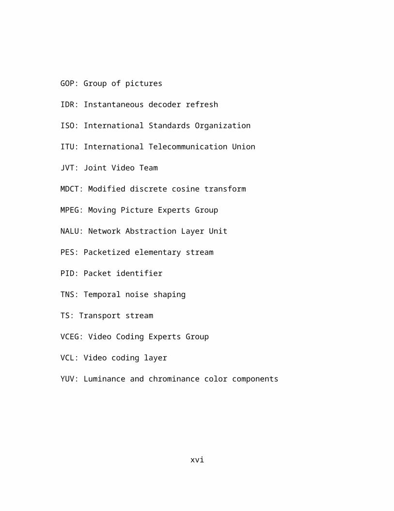
GOP: Group of pictures

IDR: Instantaneous decoder refresh

ISO: International Standards Organization

ITU: International Telecommunication Union

JVT: Joint Video Team

MDCT: Modified discrete cosine transform

MPEG: Moving Picture Experts Group

xi

NALU: Network Abstraction Layer Unit

PES: Packetized elementary stream

PID: Packet identifier

TNS: Temporal noise shaping

TS: Transport stream

VCEG: Video Coding Experts Group

VCL: Video coding layer

YUV: Luminance and chrominance color components

xii

CHAPTER 1

INTRODUCTION

1.1 Introduction

Digital television transmission has already replaced analog television

transmission with better quality and less bandwidth. With the advent of HDTV,

transmission schemes are aiming at transmitting superior quality video with provision to

view both standard format and wide screen (16:9) format along with one or more audio

streams per channel. Digital video broadcasting (DVB) in Europe and the advanced

television systems committee (ATSC) [21] in North America are working in parallel to

achieve high quality video and audio transmission. Choosing the right video codec and

audio codec plays a very important role in achieving the bandwidth and quality

requirements. H.264, MPEG-4 part-10 or AVC [5], is the latest video codec by the ITU-

T Video Coding Experts Group (VCEG) together with the ISO/IEC Moving Picture

Experts Group (MPEG) as the product of a collective partnership effort known as the

joint video team (JVT). The new standard achieved about 50% bit rate savings as

compared to earlier standards [12]. In other words, this codec provides high quality

video at the same bandwidth or same quality video in less bandwidth. H.264 provides

the tools necessary to deal with packet loss in packet networks and bit errors in error-

prone wireless networks. These features make this codec the right candidate for using in

transmission. Advanced audio coding (AAC) [1] is a standardized lossy compression 1

scheme for audio. The compression scheme was specified both as Part 7 of the MPEG-2

standard [1], and Part 3 of the MPEG-4 standard [2]. This codec showed higher coding

efficiency and superior performance at both low and high bit rates, as compared to MP3

and AC3. The video and audio streams obtained from the above mentioned codec need

to be multiplexed in order to construct a single stream, which is a requirement for

transmission. The multiplexing process mainly focuses on splitting the individual

streams into small packets, embedding information to easily realign the packets and

achieving lip sync between the individual streams, providing provision to detect and

correct bit errors and packet losses. In this thesis, the process of encoding the raw

streams, multiplexing the compressed streams followed by demultiplexing and

synchronizing the individual streams during playback, is explained in detail.

1.2 Thesis Outline

Chapter 2 and chapter 3 give an overview of the H.264 video codec and AAC

audio codec. The bit stream formats along with the reason for choosing the codec are

discussed in detail.

Chapter 4 explains the whole process of multiplexing the elementary streams

and preparing data packets for transmission. The additional information to be sent in the

packet headers to assist the demultiplexing process, are also presented in this chapter.

In Chapter 5 demultiplexing of data packets and synchronization of

reconstructed elementary streams is described. The adopted method of synchronization 2

is compared with other methods of synchronization to analyze the advantages and

disadvantages.

Chapter 6 outlines the test conditions, results and conclusions obtained using the

proposed method of implementation. Future possible improvements are also suggested.

3

CHAPTER 2

OVERVIEW OF H.264

2.1 H.264/AVC

H.264 or MPEG-4 part 10: AVC [12] is the next generation video codec

developed by MPEG of ISO/IEC and VCEG of ITU-T, together known as the JVT

(Joint Video Team). The H.264/MPEG-4 AVC standard, like previous standards, is

based on motion compensated transform coding method. H.264 also uses hybrid block

based video compression techniques such as transformation for reduction of spatial

correlation, quantization for bit-rate control, motion compensated prediction for

reduction of temporal correlation and entropy coding for reduction in statistical

correlation. The important changes in H.264 occur in the details of each functional

element. It includes intra-picture prediction, a new 4x4 integer transform, multiple

reference pictures, variable block sizes, a quarter pel precision for motion

compensation, an in-loop deblocking filter, and improved entropy coding. The new

coding tools in H.264 help achieve better coding efficiency over MPEG-2 by as much

as 3:1 in some key applications [17]. Other added features like parameter setting,

flexible macroblock ordering, switched slice, redundant slice methods along with the

data partitioning, used in previous standards, makes the standard more error resilient

compared to earlier standards.

4

The reduced bandwidth requirement due to improved coding efficiency and

improved error resilient features in H.264 make it a perfect candidate for using in video

transmission. H.264 supports various applications such as video broadcasting, video

streaming, video conferencing over fixed wireless networks and over different transport

protocols.

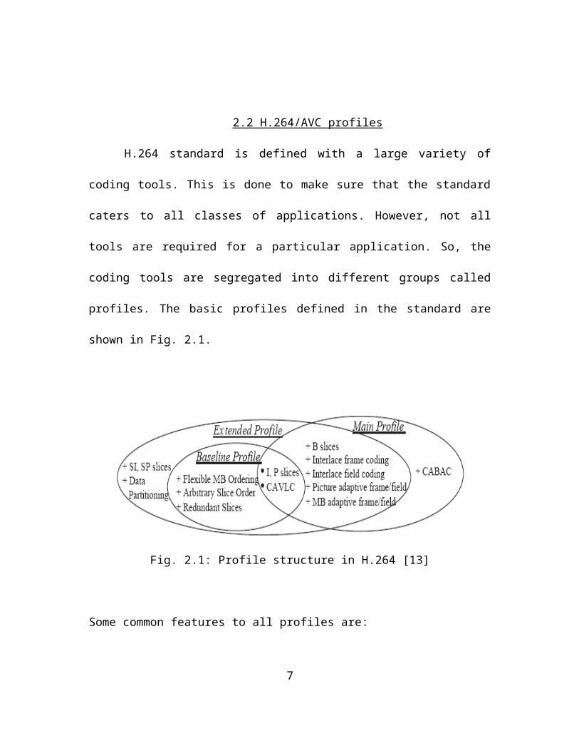
2.2 H.264/AVC profiles

H.264 standard is defined with a large variety of coding tools. This is done to

make sure that the standard caters to all classes of applications. However, not all tools

are required for a particular application. So, the coding tools are segregated into

different groups called profiles. The basic profiles defined in the standard are shown in

Fig. 2.1.

Fig. 2.1: Profile structure in H.264 [13]

5

Some common features to all profiles are:

1. Intra-coded slices (I slice): These slices are coded using prediction only from

decoded samples within the same slice.

2. Predictive-coded slices (P slice): These slices are usually coded using

interprediction from previously decoded reference pictures, except for some

macroblocks in P slices that are intra coded. Sample values of each block are

predicted using one motion vector and reference index.

3. 4X4 modified integer DCT.

4. CAVLC for entropy encoding.

5. Exponential Golomb encoding for headers and associated slice data.

The baseline profile includes I- and P-slice coding, enhanced error resilience

tools (flexible macroblock ordering (FMO), arbitrary slices and redundant slices), and

CAVLC. It was designed for low delay applications, as well as for applications that run

on platforms with low processing power and in high packet loss environment. Among

the three profiles, it offers the least coding efficiency.

The extended profile is a superset of the baseline profile. Besides tools of the

baseline profile it includes B-, SP- and SI-slices, data partitioning, and interlace coding

tools. It is thus more complex but also provides better coding efficiency. Its intended

applications are streaming video.

6

The Main profile includes I-, P- and B-slices, interlace coding, CAVLC and

CABAC. This profile was designed to provide the highest possible coding efficiency.

The features in main profile are designed to best suit the digital storage media,

television broadcasting and set-top box applications.

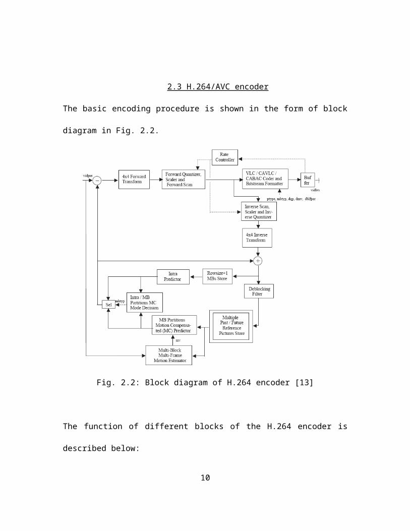
2.3 H.264/AVC encoder

The basic encoding procedure is shown in the form of block diagram in Fig. 2.2.

Fig. 2.2: Block diagram of H.264 encoder [13]

7

The function of different blocks of the H.264 encoder is described below:

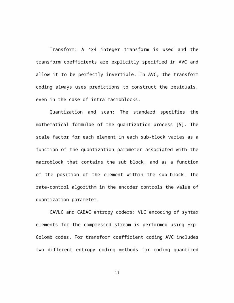
Transform: A 4x4 integer transform is used and the transform coefficients are

explicitly specified in AVC and allow it to be perfectly invertible. In AVC, the

transform coding always uses predictions to construct the residuals, even in the case of

intra macroblocks.

Quantization and scan: The standard specifies the mathematical formulae of the

quantization process [5]. The scale factor for each element in each sub-block varies as a

function of the quantization parameter associated with the macroblock that contains the

sub block, and as a function of the position of the element within the sub-block. The

rate-control algorithm in the encoder controls the value of quantization parameter.

CAVLC and CABAC entropy coders: VLC encoding of syntax elements for the

compressed stream is performed using Exp-Golomb codes. For transform coefficient

coding AVC includes two different entropy coding methods for coding quantized

coefficients of the transform. The entropy coding method can change as often as every

picture.

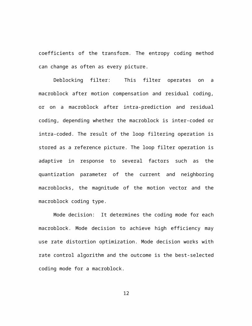
Deblocking filter: This filter operates on a macroblock after motion

compensation and residual coding, or on a macroblock after intra-prediction and

residual coding, depending whether the macroblock is inter-coded or intra-coded. The

result of the loop filtering operation is stored as a reference picture. The loop filter

operation is adaptive in response to several factors such as the quantization parameter of

8

the current and neighboring macroblocks, the magnitude of the motion vector and the

macroblock coding type.

Mode decision: It determines the coding mode for each macroblock. Mode

decision to achieve high efficiency may use rate distortion optimization. Mode decision

works with rate control algorithm and the outcome is the best-selected coding mode for

a macroblock.

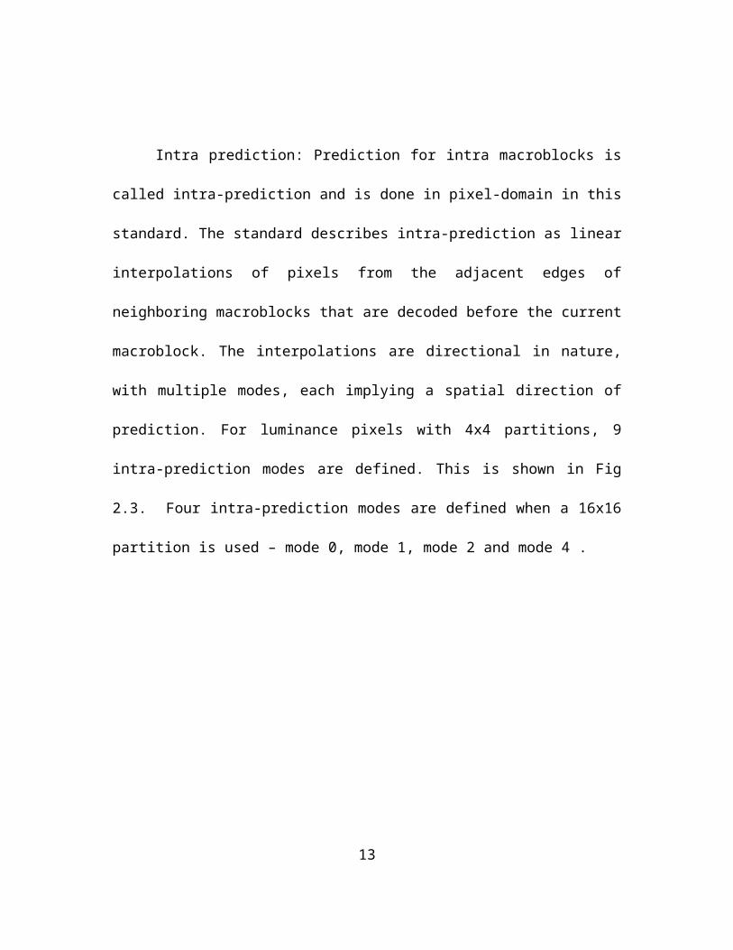
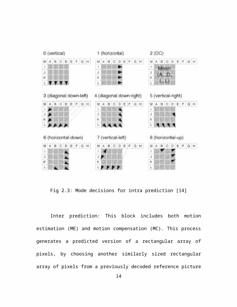
Intra prediction: Prediction for intra macroblocks is called intra-prediction and is

done in pixel-domain in this standard. The standard describes intra-prediction as linear

interpolations of pixels from the adjacent edges of neighboring macroblocks that are

decoded before the current macroblock. The interpolations are directional in nature,

with multiple modes, each implying a spatial direction of prediction. For luminance

pixels with 4x4 partitions, 9 intra-prediction modes are defined. This is shown in Fig

2.3. Four intra-prediction modes are defined when a 16x16 partition is used – mode 0,

mode 1, mode 2 and mode 4 .

9

Fig 2.3: Mode decisions for intra prediction [14]

Inter prediction: This block includes both motion estimation (ME) and motion

compensation (MC). This process generates a predicted version of a rectangular array of

pixels, by choosing another similarly sized rectangular array of pixels from a previously

decoded reference picture and translating the reference array to the position of the

current rectangular array. In AVC, the rectangular arrays of pixels that are predicted

using MC can have the following sizes: 4x4, 4x8, 8x4, 8x8, 16x8, 8x16, and

10

16x16pixels. The translation from other positions of the array in the reference picture is

specified with quarter pixel precision. In case of 4:2:0 format, chroma MVs have a

resolution of 1/8 of a pixel. They are derived from transmitted luma MVs of 1/4 pixel

resolution, and simpler filters are used for chroma as compared to luma.

IDR pictures: A special type of picture containing I-slices only called

instantaneous decoder refresh (IDR) picture is defined such that any picture following

an IDR picture does not use pictures prior to IDR picture as references for motion

prediction. Thus after decoding an IDR picture, all the following coded pictures in

decoding order can be decoded without the need to refer to any decoded picture prior to

the IDR picture. IDR pictures can be used for random access or as entry points in a

coded sequence. This plays an important role in video transmission applications.

Typically in such applications, the end user might switch to a video stream and start

decoding from any random point of time. IDR pictures forced during the encoding

process, facilitates smooth decoding of the pictures with out any propagation of error

due to lost reference frames in the bit stream.

2.4 H.264 video decoder

The decoder takes in encoded bit stream as input and gives raw YUV video frames as

output. The bit stream is first passed through the entropy decoder block which extracts

header or syntax information and slice data with motion vectors. This is followed by

inverse scan and inverse quantizer which extracts residual block data. This is in the

11

transform domain, so to bring it to the pixel domain, an inverse transform is carried out

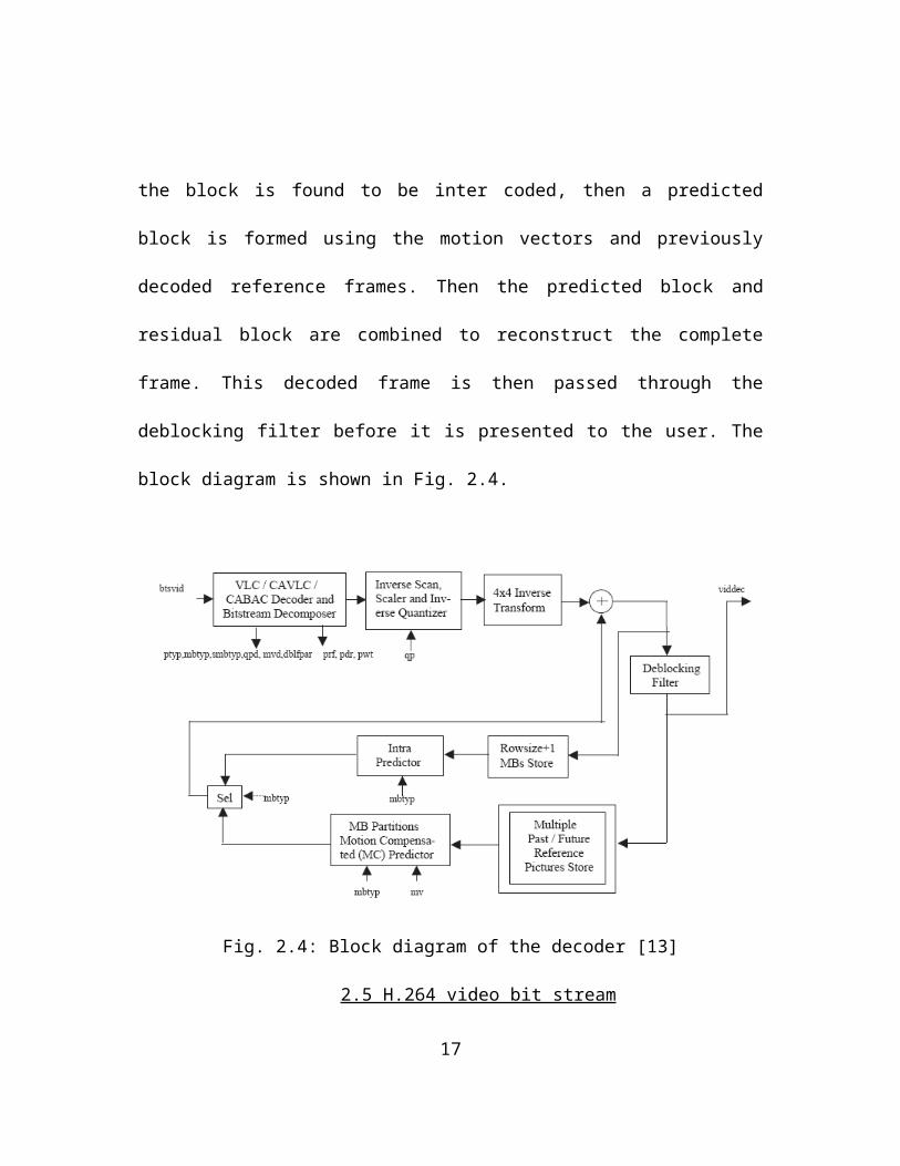
on all the blocks. If the block is found to be inter coded, then a predicted block is

formed using the motion vectors and previously decoded reference frames. Then the

predicted block and residual block are combined to reconstruct the complete frame.

This decoded frame is then passed through the deblocking filter before it is presented to

the user. The block diagram is shown in Fig. 2.4.

Fig. 2.4: Block diagram of the decoder [13]

2.5 H.264 video bit stream

The H.264 bit stream [13, 14] is broken into two layers—the video coding layer

(VCL), and the network abstraction layer (NAL). The bit stream is organized in discrete

packets, called “NAL units”, of variable length. This is an important factor that helps

12

packetize the video data into transmission packets. NAL units are separated by a simple

4-byte sequence containing a value of 1, i.e. 00 00 00 01. Thus to find a NAL unit, bit

stream has to be searched for this byte sequence. The NAL unit separators themselves

are discarded; only the following NAL unit content is processed further. VCL consists

of the bits associated with the slice layer or below - the primary domain of the

compression tools. NAL formats the compressed video data (VCL) and provides

additional non-VCL information such as, sequence and picture parameters, access unit

delimiter, filler data, supplemental enhancement information (SEI), display parameters,

picture timing etc., in a way most appropriate for a particular network/system such as

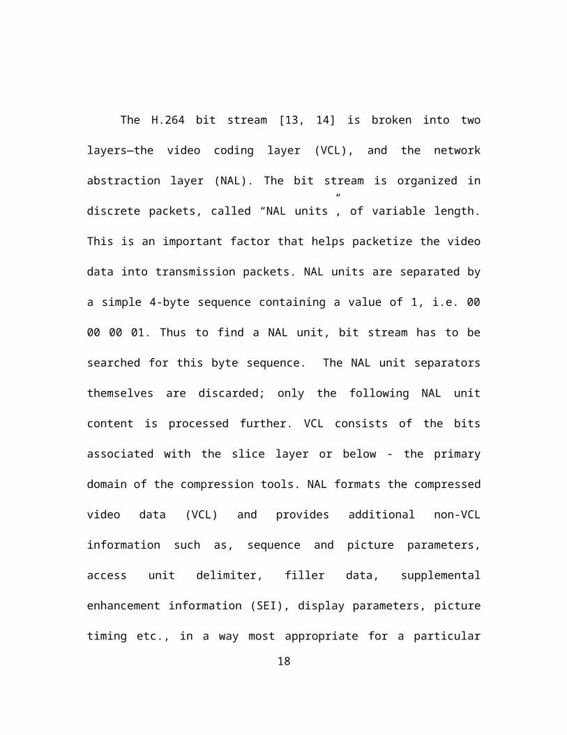
packet oriented, or bit stream oriented. Format of a NAL unit is shown in Fig. 2.5. First

byte of each NAL unit is a header byte and the rest is the data. First bit of the header is a

0 bit. Next 2 bits indicate whether the contents of NAL unit consist of sequence or

picture parameter set or a slice of a reference picture. Next 5 bits indicate the NAL unit

type corresponding to the type of data being carried in that NAL unit.

Fig. 2.5: NAL unit syntax [5 ]

There are 32 types of NAL unit allowed. The various types of NAL unit are shown in

Table. 2.1. These are classified in two categories: VCL NAL units and non-VCL NAL

13

units. NAL unit types 1–5 are VCL NAL units and contain data corresponding to the

VCL. NAL units with NAL unit type indicator value higher than 5 are non-VCL NAL

units and carry information like SEI, sequence and picture parameter set, Access Unit

Delimiter etc. NAL unit type 7 carries the sequence parameter set and type 8 carries the

picture parameter set. Depending upon a particular delivery system and scheme non-

VCL NAL units may or may not be present in the stream containing VCL NAL units.

When non-VCL NAL units are not present in the stream containing VCL NAL units,

the corresponding information can be conveyed by any external means in place in the

delivery system.

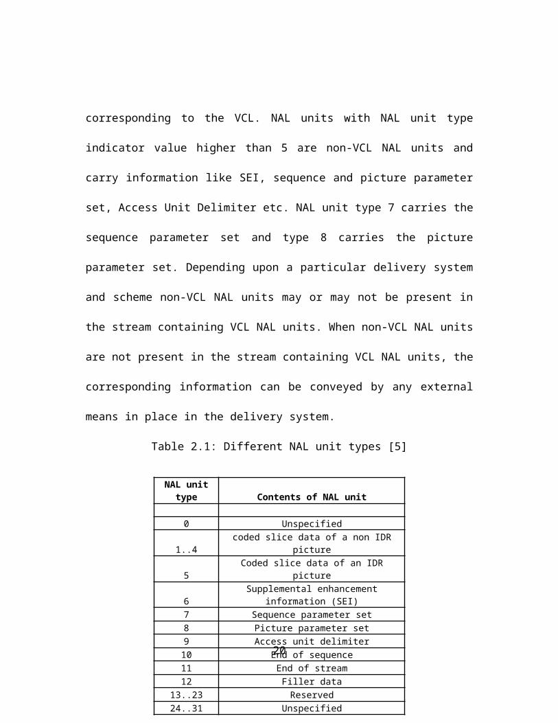
Table 2.1: Different NAL unit types [5]

NAL unit

type Contents of NAL unit

0 Unspecified1..4 coded slice data of a non IDR picture

5 Coded slice data of an IDR picture

6Supplemental enhancement information

(SEI)7 Sequence parameter set8 Picture parameter set9 Access unit delimiter

10 End of sequence11 End of stream12 Filler data

13..23 Reserved24..31 Unspecified

14

The picture parameter set and sequence parameter set play an important role

during decoding. They define some parameters of the encoded data, which are required

for decoding. So, during transmission of the video data, these two sets are sent at

frequent intervals. When the bit stream has to be decoded from any random point this

data is used along with the next IDR picture that occurs in the bit stream. Most of the

data fields of the parameter sets are stored as Exp-Golomb codes or single-bit flags. The

most important fields of a sequence parameter set are:

A profile and level indicator signalling conformance to a profile/level

combination specified in the standard.

Information about the decoding method of the picture order. Decoding order is

same as the playback order.

The number of reference frames.

The frame size in macroblocks as well as the interlaced encoding flag.

Frame cropping information for enabling non-multiple-of-16 frame sizes. These

values are ignored if the decoder always decodes full macroblocks.

Video usability information (VUI) parameters, such as aspect ratio or color

space details.

The most important fields of a picture parameter set are:

A flag indicating which entropy coding mode is used.

Information about slice data partitioning and macroblock reordering.

15

The maximum reference picture list index. This is used if long-term prediction

is enabled during encoding.

Flags indicating the usage of weighted (bi) prediction.

The initial quantization parameters as well as the luma/chroma quantization

parameter offset.

A flag indicating whether inter-predicted macroblocks may be used for intra

prediction.

2.6 Summary

In this chapter, an overview of H.264 was presented. The various profiles of the

encoder and the encoding and decoding procedures were discussed in detail. Section 2.5

elaborated on the bit stream format of the H.264 encoder .This is necessary to locate the

frame beginnings and detect the type of frames in order to packetize the data for

multiplexing and transmission which will be discussed in the later chapters.

16

CHAPTER 3

OVERVIEW OF AAC

3.1 Advanced audio coding

Advanced audio coding (AAC) [1,3] , is a combination of state-of-the-art technologies

for high-quality multichannel audio coding from four organizations: AT&T Corp.,

Dolby Laboratories, Fraunhofer Institute for Integrated Circuits (Fraunhofer IIS), and

Sony Corporation. AAC has been standardized under the joint direction of the

International Organization for Standardization (ISO) and the International Electro-

Technical Commission (IEC), as part 7 of the MPEG-2 specification. It was updated in

MPEG-4 Part 3 with a notable addition of perceptual noise substitution (PNS) in the

encoding process. Compared to the previous layers, AAC takes advantage of such new

tools as temporal noise shaping, backward adaptive linear prediction and enhanced joint

stereo coding techniques. AAC supports a wide range of sampling rates (8–96 kHz), bit

rates (16–576 kbps) and from one to 48 audio channels [9]. AAC with these

modifications from the earlier standards provides higher coding efficiency for both

stationary and transient signals. With the improved compression ratio, AAC provides

higher quality audio at the same bit rate as previous standards or same quality audio at

lower bit rates. AAC is the first codec to fulfill the ITU-R/EBU requirements for

indistinguishable quality at 128 kbps/stereo [13]. It has approximately 100% more

17

http://en.wikipedia.org/wiki/MPEG-4_Part_3

coding power than Layer II [23] and 30% more power than the former MPEG

performance leader, Layer III [13]. With all these advantages AAC replaced MP3 and

AC3 as the leading audio coding standard.

3.2 AAC profiles

The AAC system uses a modular approach. An implementer may pick and

choose among the component tools to produce a system with appropriate performance-

to-complexity ratios according to the application. This segregation is defined as

profiles. Three default profiles have been defined, using different combinations of the

available tools:

Main Profile: Uses all the encoding and decoding tools except the gain

control module. This is the most complex of the three profiles and

provides the highest quality for applications where the amount of

random accessory memory (RAM) and processing power are not

constraints.

Low-complexity Profile: Deletes the prediction tool and reduces the

temporal noise shaping tool in complexity. This profile is favorable if

memory and power constraints are to be met.

Scaleable sampling rate (SSR) Profile: Adds the gain control tool to the

low-complexity profile. Allows the least complex decoder. This profile

is most appropriate in applications with reduced bandwidth.

18

3.3 AAC encoder

The block diagram of the AAC encoder is shown in Fig. 3.1, followed by the

description of each functional block. The data flow path and control flow path are

shown by different arrows in the figure.

Fig. 3.1: AAC encoder block diagram [11]

19

Filter Bank: The first task of an audio coder is to break an audio sample into

segments, called blocks. A time domain filter, called a window, provides smooth

transitions from block to block by modifying the data in these blocks. This is done by

applying modified discrete cosine transform (MDCT) to the blocks. Choosing an

optimal block size, given the wide variety of audio material, is a problem faced by all

audio coders. AAC handles the difficulty associated with coding audio material that

vacillates between steady-state and transient signals by dynamically switching between

two block lengths: 2048-samples, and 256-samples, referred to as long blocks and short

blocks, respectively. AAC also switches between two different types of long blocks:

sine-function and Kaiser-Bessel derived (KBD) according to the complexity of the

signal.

Temporal Noise Shaping (TNS): The TNS technique provides enhanced control

of the location, in time, of quantization noise within a filter bank window. This allows

for signals that are somewhere between steady state and transient in nature. If a

transient-like signal lies at an end of a long block, quantization noise will appear

throughout the audio block. TNS allows for greater amounts of information to describe

the non-transient locations in the block. The result is an increase in quantization noise

of the transient, where masking will render the noise inaudible, and a decrease of

quantization noise in the steady-state region of the audio block. Note that TNS can be

applied to either the entire frequency spectrum, or to only a part of the spectrum, such

that the time-domain quantization can be controlled in a frequency-dependant fashion.

20

Intensity Stereo: Intensity stereo coding is based on an analysis of high-

frequency audio perception based on the energy-time envelope of the region of the

audio spectrum. Intensity stereo coding allows a stereo channel pair to share a single set

of spectral values for the high-frequency components with little or no loss in sound

quality. This is achieved by maintaining the unique envelope for each channel by means

of a scaling operation so that each channel produces the original level after decoding.

Prediction: The prediction module is used to represent stationary or semi-

stationary parts of an audio signal. Instead of repeating such information for sequential

windows, a simple repeat instruction can be passed, resulting in a reduction of

redundant information. The prediction process is based on a second-order backward

adaptive model in which the spectral component values of the two preceding blocks are

used in conjunction with each predictor. The prediction parameter is adapted on a

block-by-block basis.

Mid/Side (M/S) Stereo Coding: M/S stereo coding is another data reduction

module based on channel pair coding. In this case channel pair elements are analyzed as

left/right and sum/difference signals on a block-by-block basis. In cases where the M/S

channel pair can be represented by fewer bits, the spectral coefficients are coded, and a

bit is set to note that the block has utilized m/s stereo coding. During decoding the

decoded channel pair is de-matrixed back to its original left/right state.

Quantization and Coding: While the previously described modules attain certain

levels of compression, it is in the quantization phase that the majority of data reduction

21

occurs. This is the AAC module in which spectral data is quantized under the control of

the psychoacoustic model. The number of bits used must be below a limit determined

by the desired bit rate. Huffman coding is also applied in the form of twelve codebooks.

In order to increase coding gain, scale factors with spectral coefficients of value zero are

not transmitted.

Noiseless Coding: This method is nested inside of the previous module,

Quantization and Coding. Noiseless dynamic range compression can be applied prior to

Huffman coding. A value of +/- 1 is placed in the quantized coefficient array to carry

sign, while magnitude and an offset from base, to mark frequency location, are

transmitted as side information. This process is only used when a net savings of bits

results from its use. Up to four coefficients can be coded in this manner.

Bit stream Multiplexing: AAC has very flexible bit stream syntax. A single

transport is not ideally suited to all applications, and AAC can accommodate two basic

bit stream formats: Audio data interchange format (ADIF) and Audio data transport

stream (ADTS).

ADIF (audio data interchange format) format actually is just one header

at the beginning of the AAC file. The rest of the data are consecutive

raw data blocks. This file format is meant for simple local storing

purposes, where breaking of the audio data is not necessary.

ADTS (audio data transport stream) has one header for each frame

followed by raw block of data. ADTS headers are present before each

22

http://www.audiocoding.com/modules/wiki/?id=raw_data_block

http://www.audiocoding.com/modules/wiki/?id=AAC

AAC raw data block or block of 2 to 4 raw data blocks in a frame to

ensure better error robustness in streaming environments. Hence in this

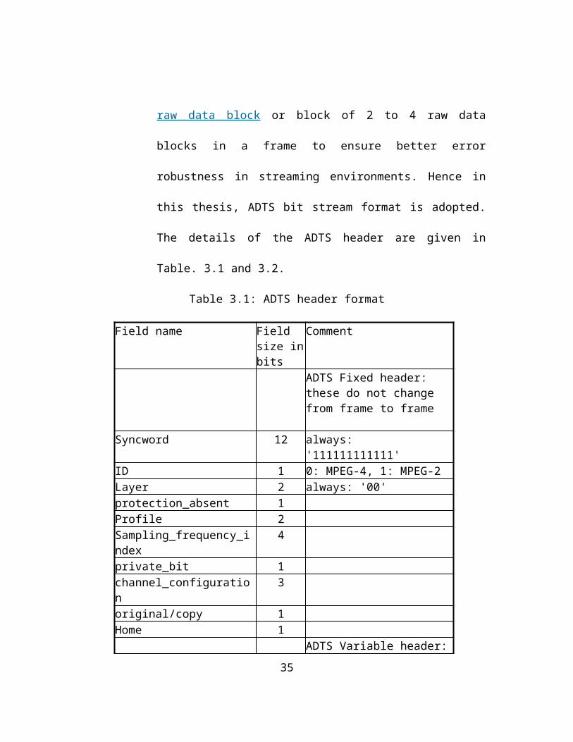
thesis, ADTS bit stream format is adopted. The details of the ADTS

header are given in Table. 3.1 and 3.2.

Table 3.1: ADTS header format

Field name Field size in bits

Comment

ADTS Fixed header: these do not change from frame to frame

Syncword 12 always: '111111111111'ID 1 0: MPEG-4, 1: MPEG-2Layer 2 always: '00'protection_absent 1Profile 2Sampling_frequency_index 4private_bit 1channel_configuration 3original/copy 1Home 1

ADTS Variable header: This can change from frame to frame

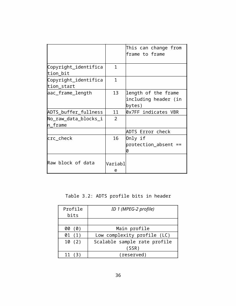
Copyright_identification_bit 1Copyright_identification_start 1aac_frame_length 13 length of the frame including

header (in bytes)ADTS_buffer_fullness 11 0x7FF indicates VBRNo_raw_data_blocks_in_frame

2

ADTS Error checkcrc_check 16 Only if protection_absent == 0

Raw block of data Variable

23

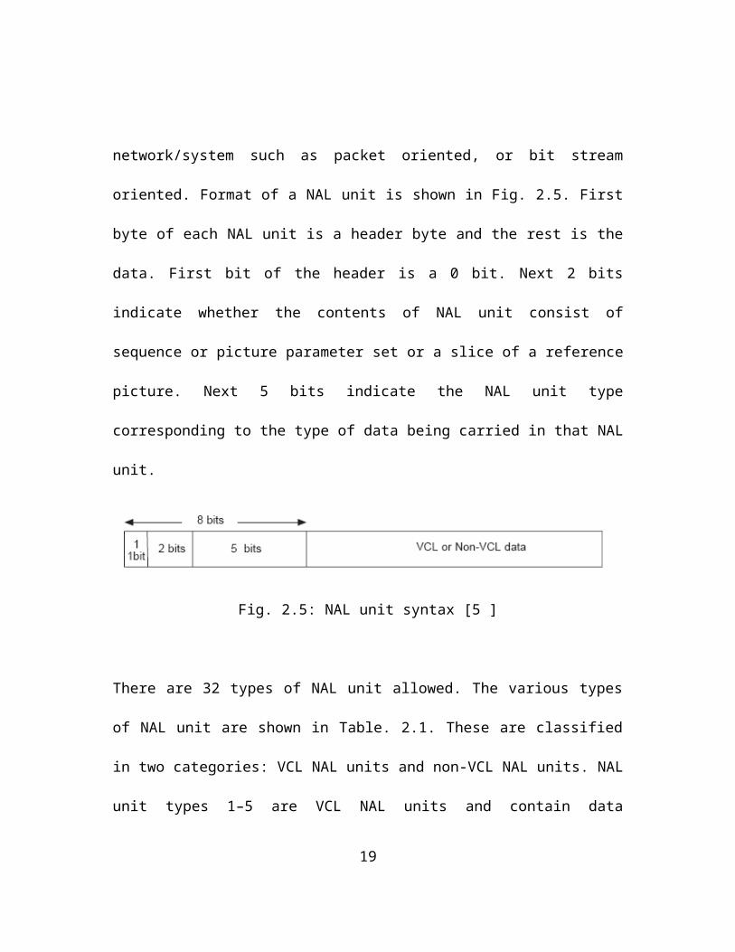
http://www.audiocoding.com/modules/wiki/?id=raw_data_block

Table 3.2: ADTS profile bits in header

Profile bits ID 1 (MPEG-2 profile)

00 (0) Main profile01 (1) Low complexity profile (LC)10 (2) Scalable sample rate profile (SSR)11 (3) (reserved)

3.4 Summary

In this chapter, the AAC audio coding standard is discussed with a detailed

description of the encoding process. The various advantages of AAC over other

standards as discussed in this chapter, explain the reason for choosing this standard for

this thesis. Low complexity profile with ADTS bit stream formatting is used in this

thesis.

24

CHAPTER 4

MULTIPLEXING

4.1 Need for multiplexing

A multimedia program consists of a combination of a few basic

elementary streams (ES) like the video stream, one or more audio streams and optional

data streams (subtitles). In case of digital television transmission standards like ATSC

[7, 21] and DVB [21] or in the case of the emerging new technology called the IPTV

[21], several of these multimedia programs need to be transmitted together as shown in

Fig. 4.1. This would mean transmitting many elementary streams together. In order to

achieve that various elementary streams need to be multiplexed in to a single

transmission stream that would carry all the data. If the application aims at delivering

high quality video and audio, then a large amount of bandwidth needs to be assigned for

transmission. This bandwidth requirement can be overcome by using highly efficient

compression schemes like the H.264 [5] scheme for video and AAC [1] scheme for

audio. This proposed method is based on MPEG-2 systems standard definitions.

Modifications have been made to the standard specifications though the framework is

similar.

25

Fig 4.1: Digital television transmission scheme

4.2 Factors to be considered for multiplexing and transmission

In order to transmit a multimedia program, a framework is to be defined which

would combine the elementary streams to form a unified bit stream. The following

factors should be considered while forming the single multiplexed bit stream. First,

while forming the single multiplexed bit stream, data from every elementary stream

should get equal priority. This is necessary to prevent any overflow or underflow of the

elementary stream buffer at the receiver side. In order to ensure this, long elementary

streams are broken down into small data packets and then multiplexed to form a single

stream of data. Formation of data packets also ensures reliable transmission. Secondly,

the multiplexed stream apart from carrying the encoded data should also contain

information to play the elementary streams in a sequence and in synchronization, in

order to make a sensible reproduction at the receiver. So, timing information needs to be

26

transmitted along with the encoded streams in the form of timestamps. Finally, if the

transmission of the bit stream takes place in an error-prone physical transmission path

like in the case of over-the-air broadcasting or cable television network, some provision

has to be made in the unified bit stream to detect these errors and correct them, if

possible.

4.3 Packetization

The first step in the process of multiplexing is packetization. This refers to

formatting the long stream of data into blocks called packets. Instead of transmitting the

data as a series of bytes, when formatted into blocks, the network can transmit a long

stretch of data more reliably and efficiently. A packet mainly consists of two parts. First

one is the header which contains the information about the data that it is carrying

followed by the payload, which is the actual data.

In the application under consideration, the data that needs to be

packetized are the audio and video streams. In case of transmitting more than one

program, we have many video and audio streams. So, during the packetization, adopted

method should be such that it would enable the user to easily realign the packets, at the

de-multiplexer side, to form the corresponding streams. In order to ensure the above

mentioned criteria and to meet the transmission channel requirements two layers of

packetization are carried out. The first layer of packetization yields the packetized

elementary stream (PES) and the second layer yields the transport stream (TS). This

27

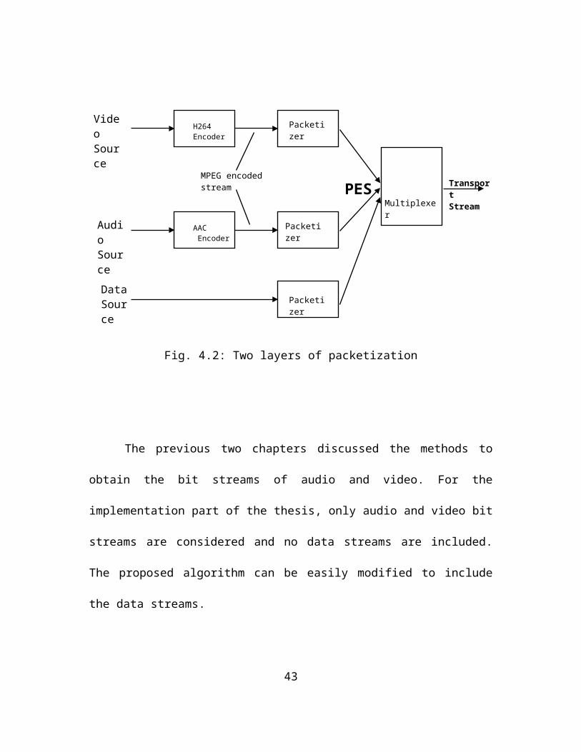
second layer is what is used for transmission. This process is shown in Fig. 4.2.

Multiplexing takes place after the second layer of packetization, just before the

transmission.

Fig. 4.2: Two layers of packetization

The previous two chapters discussed the methods to obtain the bit streams of

audio and video. For the implementation part of the thesis, only audio and video bit

streams are considered and no data streams are included. The proposed algorithm can be

easily modified to include the data streams.

H264 Encoder

AAC Encoder

Packetizer

Packetizer

MultiplexerTransportStream

VideoSource

AudioSource

MPEG encoded stream

DataSource Packetizer

PES

28

4.3.1 Packetized elementary stream

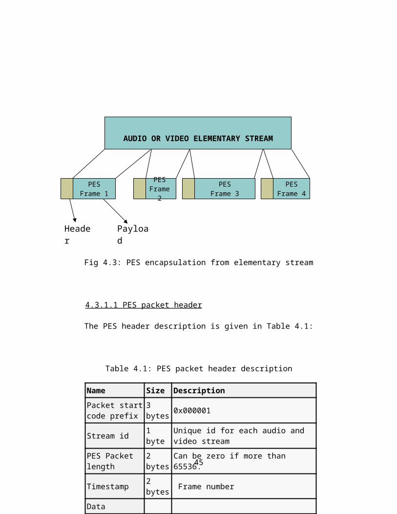
The packetized elementary stream (PES) packets are obtained by encapsulating

coded video, coded audio, and data elementary streams. This forms the first layer of

packetization. The encapsulation on video and audio data is done by sequentially

separating the elementary streams into access units. Access units in case of audio and

video elementary streams are audio and video frames respectively. Each PES packet

contains data from one and only one elementary stream. PES packets may have a

variable length since the frame size in both audio and video bit streams is variable. The

PES packet consists of the PES packet header followed by the PES packet payload. The

header information distinguishes different elementary streams, carries the

synchronization information in the form of timestamps and other useful information.

Encapsulation of elementary stream to form PES is shown in Fig 4.3.

29

Fig 4.3: PES encapsulation from elementary stream

4.3.1.1 PES packet header

The PES header description is given in Table 4.1:

Table 4.1: PES packet header description

AUDIO OR VIDEO ELEMENTARY STREAM

PESFrame 1

PESFrame 3

PESFrame 4

PESFrame 2

Header Payload

Name Size Description

Packet start code prefix 3 bytes 0x000001

Stream id 1 byte Unique id for each audio and video stream

PES Packet length 2 bytes Can be zero if more than 65536.

Timestamp 2 bytes Frame number

Data

30

PES packet length field allows explicit signaling of the size of the PES packet

(up to 65536 bytes) or, in the case of longer video elementary streams, the size may be

indicated as unbounded by setting the packet length field to zero. The frame number of

the corresponding audio and video frames in the PES packet is sent as timestamp

information in the header. This is discussed in detail in section 4.4.

4.3.1.2 PES packet payload

The PES payload is either an audio frame or a video frame data. If it is an audio

PES packet, then the AAC bit stream is searched for a 12 bit sync word of the audio

data transport stream (ADTS) format. Then the frame length is obtained from the ADTS

header, and that block of data is encapsulated with the audio stream ID to form the

audio PES packet. Audio frame number is calculated form the beginning of the stream

and the frame number is coded as the 2 byte timestamp.

If the payload has a video frame, the encoded H.264 bit stream is searched to

find the NAL unit’s prefix byte sequence of 0x00000001 which marks the beginning of

a video data set. Then the five LSB bits of the following byte are analyzed to find if the

NAL unit contains a frame, a picture parameter set or a sequence parameter set. The bit

stream syntax for this is given in Table. 2.1. The picture parameter set and sequence

parameter set carry some important information that is required by the H.264 decoder as

explained in section 2.5. So in order to facilitate decoding from any IDR frame, these

two NAL units need to be transmitted at regular intervals. So, the picture parameter set

31

and the sequence parameter set, if found in the bit stream, are combined to form a

separate PES with frame number zero. Instead if the NAL unit contains IDR, P or B

slice data, then the frame number is calculated from the beginning of the stream and is

encapsulated as a timestamp along with the video stream ID and frame length.

The PES has an 8 byte header and variable size payload. In an error-prone

transmission channel fixed size packets are more desirable, since it is easier to detect

and correct errors. So, this requires the data to be put through one more layer of

packetization in order to obtain fixed size packets that can be used for transmission.

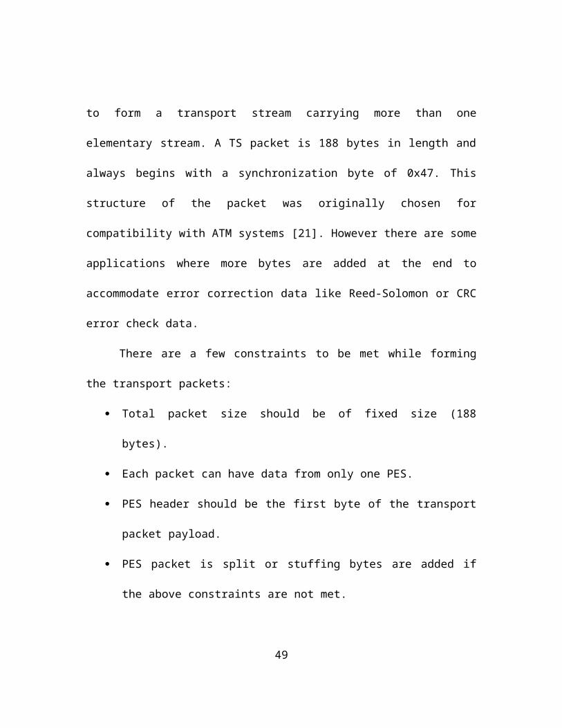
4.3.2 Transport stream

The second layer of packetization forms a series of packets called the transport

stream (TS). These are fixed length subdivisions of the PES packets with additional

header information. These packets are multiplexed together to form a transport stream

carrying more than one elementary stream. A TS packet is 188 bytes in length and

always begins with a synchronization byte of 0x47. This structure of the packet was

originally chosen for compatibility with ATM systems [21]. However there are some

applications where more bytes are added at the end to accommodate error correction

data like Reed-Solomon or CRC error check data.

There are a few constraints to be met while forming the transport packets:

Total packet size should be of fixed size (188 bytes).

Each packet can have data from only one PES.

32

PES header should be the first byte of the transport packet payload.

PES packet is split or stuffing bytes are added if the above constraints are not

met.

The encapsulation of PES packets to form TS packets is shown in Fig 4.4.

PES PayloadPES Header

Transport Header

Transport StreamPacket

Stuffing bytesPayload

Fig 4.4: TS packet formation from PES packet

4.3.2.1 TS packet header

The TS packet normally consists of a 3 byte header. However, if adaptation field

is present, then an additional byte is added to the header and 184 bytes are available for

payload including the adaptation field. The header structure of the TS packet is given in

Table 4.2 and following that the description of the syntax is given.

33

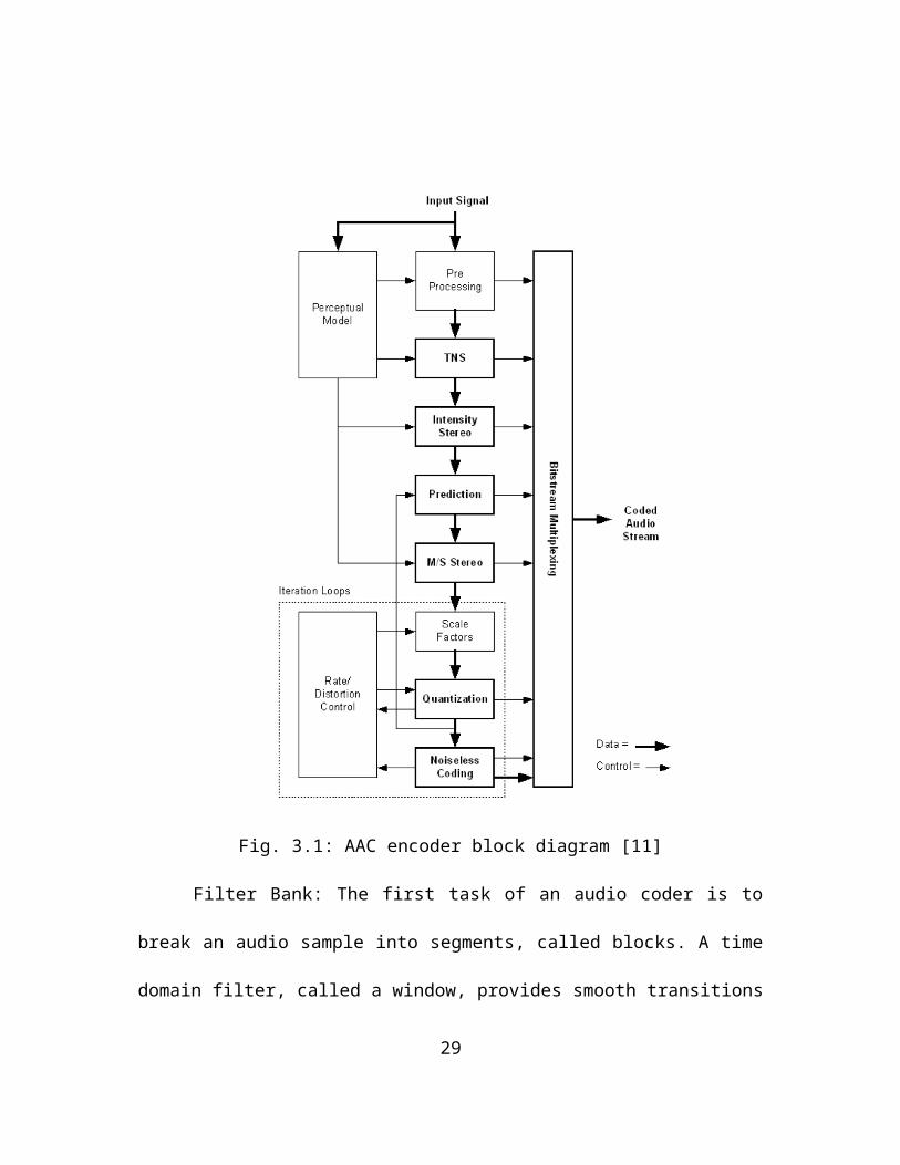
Table 4.2: TS packet header description

Syntax Number of bits

sync byte 8

Payload unit start indicator 1

adaptation field control 1

PID 10

Continuity Counter 4

if adaptation field control = =1

payload byte offset 8

stuffing bytes or additional header

payload

Payload unit start indicator:

This bit is set to indicate to the demultiplexer that the first byte of the PES

packet is present in the payload of the current transport stream packet.

Adaptation field control:

This bit is set, if the payload of the current TS packet contains information other

than the PES data. This can be a stretch of stuffing bytes (0xff) in case the PES

data is not long enough to fill the TS packet or any other additional data

regarding the payload. The block of data occupied by this additional information

is called as adaptation field and is stored just after the header before the payload.

34

PID (Packet identifier) :

Each TS packet contains a 10 bit packet identifier called PID. This is used to

uniquely identify the elementary stream to which the data in the packet belongs,

when generated by the multiplexer. The PID allows the receiver to differentiate

the stream to which each received packet belongs. Some PID values are

predefined and are used to indicate various streams of control information. A

packet with an unknown PID, or one with a PID which is not required by the

receiver, is discarded. The particular PID value of 0x1024 is reserved to indicate

that the packet is a null packet and is to be ignored by the receiver.

Continuity counter :

This is a 4 bit rolling counter which is incremented by 1 for each consecutive TS

packet of the same PID. This is provided to aid the demultiplexer to detect any

packet losses during transmission.

Payload byte offset :

If adaptation field control bit is set to 1, byte offset value of the start of the

payload or the length of adaptation field is mentioned here.

Null packets:

This type of TS packets just contains stuffing bytes all through out the payload.

They do not carry any useful information. These packets are generally used in

transmission channels that require constant bit rate at all times. In such cases if

the TS packets from the PES are not ready for transmission, these null packets

35

are sent just as a filling to keep a constant bit rate. These packets have a unique

PID and are directly rejected upon reception at the demultiplexer.

4.4 Frame number as timestamp

The proposed method uses the frame number as timestamps. This section

explains how frame numbers can be used to synchronize audio and video streams. Both

H.264 and AAC bit streams are composed of data blocks sorted into frames. A

particular video bit stream has a constant frame rate during playback specified by

frames per second (fps). So, given the frame number, one can calculate the time of

occurrence of this frame in the video sequence during playback as follows:

Time of playback = Frame number /fps (4-1)

The AAC compression standard defines each audio frame to contain 1024 samples. The

audio data in the AAC bit stream can have any discrete sampling frequency between 8 –

96 kHz. The frame duration increases from 96 kHz to 8 kHz. However, the sampling

frequency and hence the frame duration remains constant throughout a particular audio

stream. So, the time of occurrence of the frame during playback is as follows:

Time of playback = 1024*frame number/(sampling freq). (4-2)

36

Thus from (4-1) and (4-2) we can find the time of playback by encoding the

frame numbers as the time stamps. In other words, given the frame number of one

stream, we can the find the frame number of the other streams that will be played at the

same time as the frame of the first stream. This will help us synchronize the streams

during playback. This idea can be extended to synchronize more than one audio stream

with the single video stream like in the case of stereo or programs with single video and

multiple audio channels.

The timestamp is assigned in the last 2 bytes of the PES packet header. This

implies that timestamp can carry frame numbers up to 65536. Once the frame number

exceeds this, in the case of long video and audio streams, the frame number is rolled

over. The rollover takes simultaneously on both audio and video frame numbers as soon

as either one of the stream crosses the maximum allowed frame number. This will not

create a conflict at the demultiplexer during synchronization because the audio and

video buffer sizes are much smaller than the maximum allowed frame number. So, at no

point of time there will be two frames in the buffer with the same timestamp.

4.4.1 Advantages of frame numbers over clock samples as timestamps

The other method that is used to synchronize audio and video involves using

clock samples as timestamps. A master clock is generated at the multiplexer and the

samples of this clock are sent in the packet header to determine when the frame is to be

presented. The master clock is regenerated at the receiver and the clock samples are

37

compared before presentation to achieve synchronization. For this to work reliably, the

clocks at the multiplexer and demultiplexer should be absolutely synchronized. In order

to achieve this, additional information about the reference clock needs to be sent at

regular intervals of time. Eventually, the timestamps are compared to the regenerated

master clock before presentation and the individual streams are synchronized. The

advantages of using frame numbers over clock samples as time stamps are:

Less complex and more suitable for software implementation.

Saves the extra PES header bytes used for sending the program clock reference

(PCR) information periodically.

No synchronization problem due to clock jitters or inaccurate clock samples.

No propagation of delay between audio and video due to drift between the

master clocks at the transmitter and receiver.

4.5 Proposed multiplexing method

The final transmission stream is formed by multiplexing the TS packets of the

various elementary streams. The number of packets allocated for a particular elementary

stream during transmission, plays an important part in avoiding buffer overflow or

underflow at the demultiplexer. If more video TS packets are sent as compared to audio

TS packets, then at the receiver there might be a situation when video buffer is full and

is overflowing whereas audio buffer does not have enough data. This will prevent the

38

demultiplexer from starting a playback and will lead to loss of data from the

overflowing buffer.

In order to prevent such a scenario, timing counters are employed at the

multiplexer. Each elementary stream has a timing counter, which gets incremented

when a TS packet from that elementary stream is transmitted. The increment value

depends on the playback time of the TS packet. The playback time of each PES can be

calculated since the frame duration is constant in both audio and video elementary

streams. By finding out how many TS packets are obtained form a single PES packet,

the playback time of each TS packet can be calculated. This is shown graphically in Fig.

4.5. The elementary stream whose counter has the least timing value is always given

preference in packet allocation. This method will make sure that at any point of time,

the difference in the fullness of the buffers, in terms of playback time is less than the

playback time of one TS packet. This is never more than the duration of a single frame

and is typically in milliseconds. There are other methods of multiplexing proposed in

various references. One of which calculates the ratio of file sizes of the video and audio

files and keeps the same ratio for the number of TS packets added from the elementary

streams [6]. However, this is not a dynamically changing method that can adopt to the

varying frame sizes of the elementary streams. Also, this method requires us to have the

full size of the files before beginning the multiplexing process. This might not be

possible if encoding is done in real time.

39

Video PES => 1/25 = 40 ms

Fps = 25

4 TS packets

=> 40/4 = 10 ms# of TS = round(570/185)

PES length = 570

Fig. 4.5: Calculation of playback time of a TS packet

4.6 Summary

In this chapter, the proposed multiplexing process is discussed in detail. The two

layers of packetization carried out on elementary streams and the various header

information embedded during this process are described. A description is given on how

frame numbers can be used as timestamps to achieve lip sync between audio and video.

This method is compared with other synchronization method that uses clock samples as

timestamps. Eventually, a method for multiplexing the TS packets is proposed that

would prevent buffer overflow or underflow at the demultiplexer.

40

CHAPTER 5

DEMULTIPLEXING AND SYNCHRONIZATION

5.1 Demultiplexing

The process of recovering the elementary streams from the multiplexed

transport stream is called demultiplexing. This is the first step carried out at the

receiver, in the process of delivering a complete multimedia program to the end user.

The flowchart of the demultiplexer algorithm is given in Fig 5.1.

Fig. 5.1: Flowchart of the demultiplexer

41

Upon receiving the packets, their corresponding PID values are extracted. If the

packet has any PID value that is not relevant to the multimedia program that is being

recovered, the packet is dropped and the next packet is analyzed. All the TS packets

from other programs or null packets are eliminated at this stage. This is done to prevent

using the resources on unwanted data. Once the packet has been identified to be a

required one, further analysis of the packet is carried out. The ‘adaptation field control’

bit is checked to see if any data other than the elementary stream data is present in the

packet. If yes, then the essential data is recovered from the payload starting from the

byte obtained by reading the ‘byte offset value’ from the header. The remaining data is

rejected if it is filled with stuffing bytes. The data is identified to be audio data or video

data through the PID value and is redirected to the appropriate buffer. The packet is also

analyzed to check if the ‘payload unit start’ bit is set. If it is set, then the PES header is

present in the packet. The header information is read to recover the frame length and

timestamp, which is the frame number. The frame number and location of the frame in

the data buffer are stored in a separate buffer. This process is continued until one of the

elementary stream buffers is full. In order to detect packet losses, 4 bit continuity

counter value is continuously monitored for each PID separately, to check if the counter

value increments in sequence. If not a packet loss is declared and the particular frame in

the buffer, which is involved in the loss, is marked to be erroneous. In some

transmission schemes, retransmission of the packet is requested to correct the error.

Otherwise, the frame is skipped during playback to prevent any stall in the decoder.

42

It is important to continuously monitor the fullness of the elementary stream

buffers. The buffer should not be allowed to overflow or underflow. This will lead to

loss of data. This is taken into account during the multiplexing process as explained in

section 4.4. Table 5.1 gives the details of the buffer at the demultiplexer, as observed

during the actual implementation of the proposed method. Table 5.2 gives the results

obtained by using the ratio of total video and audio file sizes as the multiplexing

criteria. The ratio was found to be 3:1. So, constant multiplexing method was adopted in

which three video TS packets followed by an audio TS packet, is sent in the multiplexed

stream.

Table 5.1: Buffer fullness at demultiplexer using proposed method

Test criteria

Buffer details

Video buffer 100kB

Video buffer 600kB

Video buffer 600kB

Start TS packet number 1 1 3850

End TS packet number 802 4341 7928

Video buffer fullness (kB) 100 600 600

Audio buffer fullness (kB) 33 140 119

Number of video frames 43 211 173

Number of audio frames 82 397 326Video buffer content playback time 1.72 sec 8.44 sec 6.92 secAudio buffer content playback time 1.75 sec 8.47 sec 6.95 sec

43

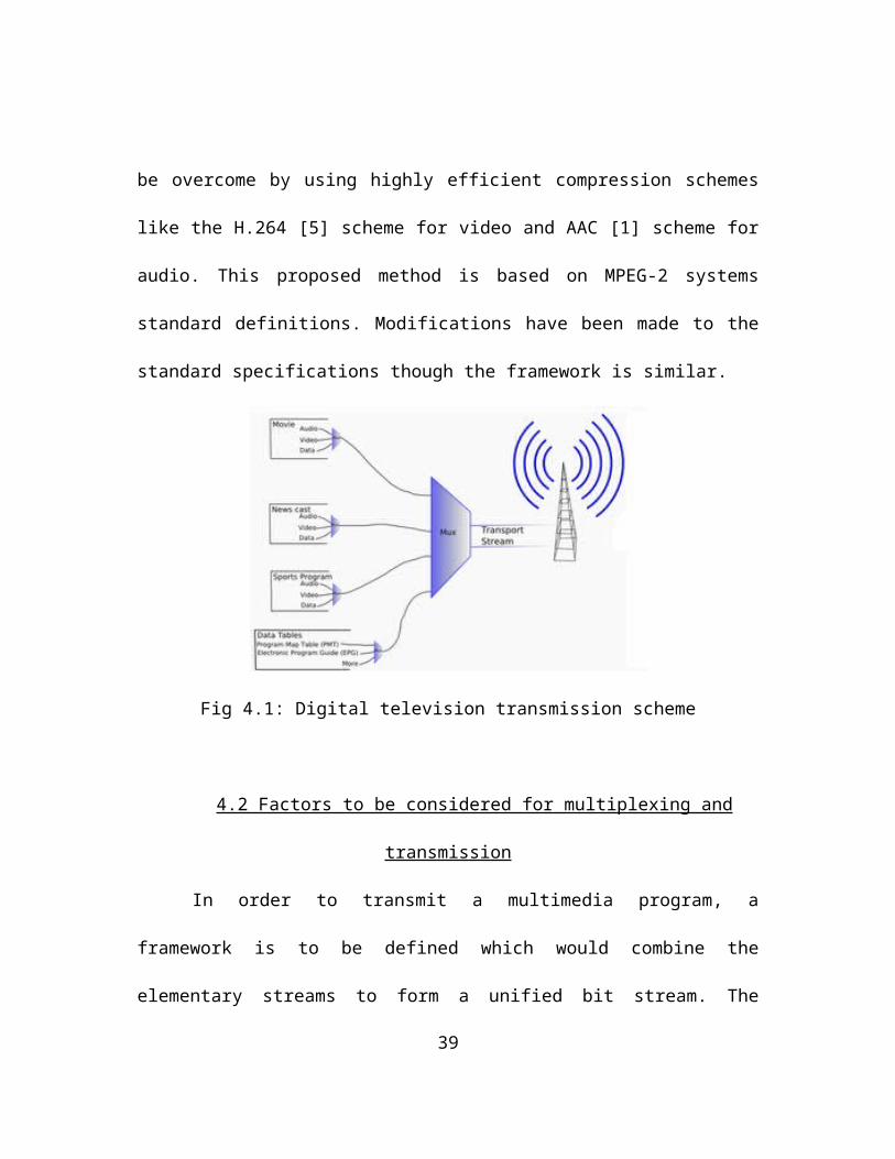
Table 5.2: Buffer fullness at demultiplexer using alternative method

Test criteria

Buffer details Video buffer

100kB Video buffer

600kB Video buffer

600kB

Start TS packet number 1 1 3850

End TS packet number 758 4478 8297

Video buffer fullness (kB) 100 600 600

Audio buffer fullness (kB) 24.5 128 119

Number of video frames 44 212 170

Number of audio frames 95 642 493Video buffer content playback time 1.76 sec 8.48 sec 6.8 secAudio buffer content playback time 2.03 sec 13.7 sec 10.52 sec

The first table clearly shows that the audio and video buffer fullness, using the proposed

method has nearly the same amount of playback time, irrespective of the buffer size or

the TS start packet during demultiplexing. The difference is very small. This enables us

to playback the content as soon as one of the buffers gets filled and starts refilling the

buffer with new content. However, the alternative method that used the method

specified in reference [6] has uneven buffer fullness. As we see from the table, the

difference in buffer fullness varies as we increase the size of the buffer, and also if we

change the starting TS packet number. If this continues then there might be buffer

overflow or underflow. This however is not the case with the proposed method which

44

dynamically adjusts the multiplexing process and hence shows superior performance as

compared to the other methods in maintaining the buffer fullness.

5.2 Synchronization and playback

Once the elementary stream buffer is full, the content is ready to be played back

for the viewer. The audio bit stream format i.e., audio data transport stream (ADTS),

enables us to begin decoding form any frame. However, the video bit stream does not

have the same kind of sophistication. The decoding can start only from the anchor

frames, which are the IDR frames. As explained in chapter 3, IDR frames are forced

during the encoding process at regular intervals. So, the video buffer is first searched

from the top to get the first occurring IDR frame. Once this is found, the timestamp or

the frame number is obtained for that IDR frame. Then audio stream is aligned

accordingly to achieve synchronization. This is done by calculating the audio frame

number that would correspond to the IDR frame in terms of playback time. This is

calculated as follows:

Audio frame number = (5-1)

If the frame number calculated is a non-integer value, then the value is rounded off and

the corresponding frame is taken. The round off error is discussed later in this chapter.

If the calculated frame number is not found in the buffer, next IDR frame is searched

45

and a new audio frame number is calculated. Once video frame number and audio frame

number are obtained, the location of these frames is looked up in the buffer and the

block of data from this frame to the end of the buffer is taken and sent to the decoder for

playback. The buffer is then emptied and the incoming data is filled in the buffer and

the process is repeated. In order to have a continuous playback, block of data from first

IDR frame to last IDR frame in the buffer is played back and during this playback the

next set of data buffering takes place in the background. This process continues and the

program is continuously played for the viewer.

As explained in the previous section, when the calculated audio frame is

not an integer value it is rounded off. So mathematically, the maximum error will be

equal to 0.5 times the duration of an audio frame. This is determined by the sampling

frequency of the audio stream. For most sampling frequencies the audio frame duration

is not more than 64 ms so the maximum error is about 30 ms. The MPEG-2 systems

standard allows a maximum time difference between audio and video streams of 40 ms

[3]. So the rounded value is just taken as the required frame number. However, if the

maximum possible delay due to round off error is more than 40 ms, then the first IDR

frame is repeated which makes up for 40 ms (25 fps). If the audio leads video, then the

previous audio frame is taken. This reduces the delay between audio and video to less

than 40ms. Once synchronized, the delay remains constant from then on through out the

playback time. The possible delay between audio and video streams is a limitation for

this method. However, this delay is very small and is not perceptible. Still, if the round

46

off error leads to a delay of more than 40 ms, then the next IDR frame in the buffer is

searched and that new frame number is used for synchronization. Once the buffer is full

and the synchronized frames are calculated, the audio and video content are played

back. This is done by using the VLC media player software [35], which is a public

software program distributed by the videolan project group. The buffering is continued

after the playback and next set of data is put through the same process. This process

continues and thus successful demultiplexing and synchronized playback is achieved.

This completes the process of multiplexing, demultiplexing and a synchronized

playback of multimedia programs. There is no open literature or any standard developed

to carry out this process. Currently, the implementation is only in the industries and the

documentation of the implementation procedure is not freely available. This makes it

very difficult to draw a comparison between the proposed method and other existing

methods.

5.3 Summary

In this chapter, the process of extracting data form the multiplexed TS packets,

to reconstruct the elementary stream is explained in detail. Then an analysis of how the

multiplexing process helps in maintaining the buffer fullness at the demultiplexer is

given. Synchronization and playback method using frame numbers as timestamps are

proposed and the limitations due to possible error in synchronization are discussed.

47

CHAPTER 6

RESULTS AND CONCLUSION

6.1 Implementation and results

The proposed multiplexing method was implemented with a single program

stream comprising of a video elementary stream and an audio elementary stream, each

worth 130 seconds of playback. To begin with, the elementary streams are in raw

formats, with video stream in the YUV format and audio stream in the WAVE format.

There are no standard video and corresponding audio test sequences, freely available,

that can be used for implementation. Hence these raw sequences were extracted from

the existing AVI file format using ffmpeg [36] software. This is an open source

software, which helps extract YUV format video and wave format audio from any AVI

format. This extracted video stream is encoded using the 10.2 JM, H.264 encoder [27].

The main profile is used for encoding, since it is more suitable for transmission

applications as explained in section 2.2. The GOP sequence adopted during the

encoding process is IBBPBB, where I is an IDR frame. The audio stream is encoded

using the free advanced audio coder (FAAC) [24]. The audio stream is a encoded in

low-complexity profile. The encoded streams are then multiplexed to form the TS

packets. The details of both, the clips and the multiplexed stream, are given in Table.

6.1.

48

Table 6.1: Results of multiplexed stream on test clip

Test Clip Details Clip 1 Clip 2

Duration of clip (sec) 125 56

Audio Frequency (Hz) 48,000 11,025

Video frame rate (fps) 25 25

YUV file size (kB) 468,168 150,075

WAVE file size (kB) 25,624 957

H.264 file size (kB) 6,566 4,551

AAC file size (kB) 2,066 149

Video coder Compression ratio 71.30 32.98

Audio coder Compression ratio 12.40 6.42

H.264 encoder bit rate (kBps) 52.53 81.27

AAC encoder bit rate (kBps) 16.53 3.38

Number of TS packets 50,577 26,872

Total transport stream size (kB) 9,508 5,051Compression ratio with header overhead 51.93 29.90

Bit rate for transmission (kBps) 76.06 90.20

AVI (*.avi) file size (kB) 19,456 14,311MPEG-2 movie (*.mpg) file size (kB) 15,666 12,036

49

The results on the table clearly show that the compression achieved, using

H.264 video codec and AAC audio codec, in the proposed method is more than that of

the MPEG-2 movie files (.mpg) or AVI files. This is true even with the packet header

overheads included. The bit rate required for transmission depends heavily on the bit

rates chosen by the audio and video encoders. The final bit rate can be varied to suit the

transmission channel, by changing the rate control parameter in the H.264 encoder.

Then the TS packets are given as the input to the proposed demultiplexer

algorithm to achieve synchronized playback. It is verified to see if synchronization

between audio and video is achieved, irrespective of which TS packet the user starts

demultiplexing from. So, some random TS packets are chosen to begin the

demultiplexing process and the results of the synchronization process are given in Table

6.2. The delay between audio and video is less than 6 milliseconds in the observed

cases. This delay remains constant throughout the playback time once synchronized.

Table 6.2: Observed synchronization delay on test clip

Start TS packet number

Synchronized frame numbers chosen

Video frame playback time (sec)

Audio frame playback time (sec)

Delay(msec)

Visual delay

Video Audio

120 18 34 0.72 0.725 5.22Not perceptible

2000 102 191 4.08 4.074 5.97Not perceptible

6000 282 529 11.28 11.284 3.57Not perceptible

23689 1308 2453 52.32 52.322 2.49Not perceptible

45250 2826 5299 113.04 113.045 5.33Not perceptible

50

6.2 Conclusions

This thesis is focused on creating an effective transport stream that would carry

multiple elementary streams and deliver a synchronized multimedia program to the

receiver. This is achieved by adopting 2 layers of packetization of the elementary

stream followed by a multiplexing procedure. The proposed multiplexing procedure

enables the user to start demultiplexing from any TS packet and achieve synchronized

playback for any program. There is also provision for error detection and correction

after receiving the packets. These are absolutely essential for video broadcasting

applications. Usage of H.264 video bit stream and AAC audio bit stream helps transmit

high quality audio-video at lesser bit rates. This meets all the basic requirements to

transmit a high quality multimedia program.

6.3 Future research

The implementation of the proposed algorithm is directed towards multiplexing

two elementary streams that would constitute a single program. However, it can be

easily modified to include more streams and can be used to transmit multiple programs

together.

For television broadcasting applications, error resilience is an important factor.

Though the proposed algorithm gives provision to add error correction codes, this was

not adopted in the implementation. With minor additions to the code, some robust error

correction codes can be integrated to the transport packets, to make them more suitable

for such applications.

51

REFERENCES

[1]MPEG–2 advanced audio coding, AAC. International Standard IS 13818–7, ISO/IEC

JTC1/SC29 WG11, 1997.

[2]MPEG. Information technology — generic coding of moving pictures and associated

audio information, part 3: Audio .International Standard IS 13818–3, ISO/IEC

JTC1/SC29 WG11, 1994.

[3]MPEG. Information technology — generic coding of moving pictures and associated

audio information, part 4: Conformance testing .International Standard IS 13818–4,

ISO/IEC JTC1/SC29 WG11, 1998.

[4]Information technology—Generic coding of moving pictures and associated audio—

Part 1: Systems, ISO/IEC 13818-1:2005, International Telecommunications Union.

[5] MPEG-4: ISO/IEC JTC1/SC29 14496-10: Information technology – Coding of

audio-visual objects - Part 10: Advanced Video Coding, ISO/IEC, 2005.

[6] P. V. Rangan, S. S. Kumar, and S. Rajan, “Continuity and Synchronization in

MPEG,” IEEE Journal on Selected Areas in Communications, Vol. 14, pp. 52-60, Jan.

1996.

[7] B.J. Lechner et. al “The ATSC Transport Layer, Including Program and System

Information Protocol (PSIP)”, Proc of the IEEE, vol. 94, no. 1,pp 77-101, January 2006

52

[8] Hari Kalva et. al “Implementing Multiplexing, Streaming,and Server Interaction for

MPEG-4”, IEEE transactions on circuits and systems for video technology, vol 9, No.8,

pp 1299-1311,december 1999.

[9] M. Bosi and M. Goldberg “Introduction to digital audio coding and standards”,

Boston : Kluwer Academic Publishers, c2003.

[10] D. K. Fibush, “Timing and Synchronization Using MPEG-2 Transport Streams,”

SMPTE Journal, pp. 395-400,July, 1996.

[11]K. Brandenburg, “MP3 and AAC Explained”, AES 17th International Conference,

Florence, Italy, September 1999.

[12] S-k. Kwon, A. Tamhankar and K.R. Rao ”Overview of H.264 / MPEG-4 Part 10”,

J. Visual Communication and Image Representation, vol. 17, pp.183-552, April 2006.

[13]A. Puri, X. Chen and A. Luthra, “Video coding using the H.264/MPEG-4

AVC compression standard”, Signal Processing: Image Communication, vol. 19, issue

9, pp. 793-849, Oct 2004.

[14] T. Wiegand et. al “Overview of the H.264/AVC Video Coding Standard,” IEEE

Trans. CSVT, Vol. 13, pp. 560-576, July 2003.

[15] R. Hopkins, “United States digital advanced television broadcasting standard,”

SPIE/IS & T, Photonics West, vol. CR61,pp 220-226, San Jose, CA, Feb. 1996.

[16] Z. Cai et. al “A RISC Implementation of MPEG-2 TS Packetization”, in the

proceedings of IEEE HPC conference, pp 688-691, May 2000.

53

[17] M.Fieldler, “Implementation of basic H.264/AVC Decoder”, seminar paper at

Chemnitz university of technology, June 2004

[18] R.Linneman, “Advanced audo coding on FPGA”, BS honours thesis, October

2002, School of Information Technology, Brisbane.

[19] J. Watkinson, “The MPEG Handbook” , Second Edition , Oxford ; Burlington, MA

: Elsevier/Focal Press, 2004.

[20] I.E.G.Richardson, “H.264 and MPEG-4 Video Compression: Video Coding

for Next Generation Multimedia”, John Wiley & Sons, 2003.

[21]Proceedings of the IEEE, Special issue on Global Digital Television: Technology

and Emerging Services, vol.94,pp 5-7, Jan. 2006.

[22] P.D Symes “Digital video compression“, McGraw-Hill, c2004

[23] C. Wootton, “Practical guide to video and audio compression : from sprockets and

rasters to macro blocks”, Oxford : Focal, 2005.

[24] “FAAC and FAAD AAC software, website

www.audiocoding.com

[25] MPEG official website

www.mpeg.org

[26] Alternative AAC software from

http://www.psytel-research.co.yu

[27] H.264 software JM (10.2) from

http://iphome.hhi.de/suehring/tml/

54

http://iphome.hhi.de/suehring/tml/

http://www.psytel-research.co.yu/

http://www.mpeg.org/

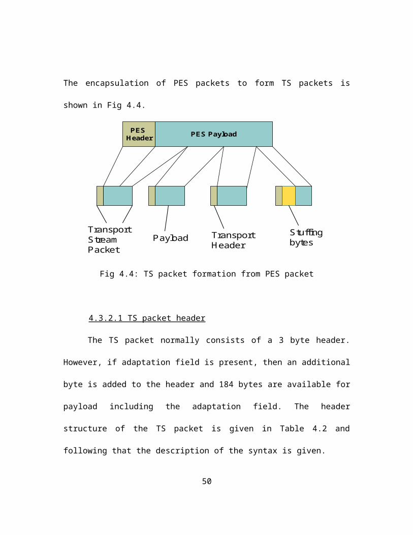
[28] Bauvigne G. “MPEG-2/MPEG-4 AAC”, MP3 Tech Website,

www.mp3-tech.org

[29] Whittle R., “Comparing AAC and MP3”, Website

http://www.firstpr.com.au/audiocomp/aac-mp3-vq.html

[30] Public discussion forum website for a/v containers:

http://forum.doom9.org/forumdisplay.php?s=c68a3cd483892abb630cf026aa06d3c5&f

[31] Public discussion forum for MPEG

http://forum.doom9.org/forumdisplay.php?f=77

[32] JVT documents website:

http://www.dspr.com/www/technology/JVT-G050.pdf

[33]Audio test files website

http://www.rme-audio.com/english/download/audtest.htm

[34]Reference for H.264 website

http://www.vcodex.com/h264.html

[35] VLC software and source code website

www.videolan.org

[36] Ffmpeg software and official website

http://ffmpeg.mplayerhq.hu/

55

http://ffmpeg.mplayerhq.hu/

http://www.videolan.org/

http://www.vcodex.com/h264.html

http://www.rme-audio.com/english/download/audtest.htm

http://www.dspr.com/www/technology/JVT-G050.pdf

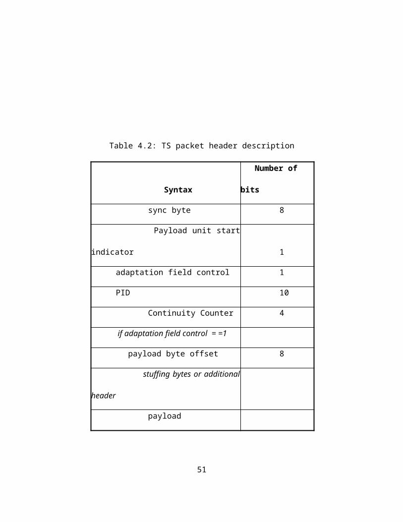
BIOGRAPHICAL INFORMATION

Harishankar Murugan received his Bachelor of Engineering degree in Electrical

Engineering from Mumbai University, India, in June 2005. He pursued his masters

studies at the University of Texas at Arlington from august 2005 and received his M.S

degree in Electrical Engineering in May 2007. He was a member of the multimedia

processing research group guided by Dr. K. R. Rao. He worked as an intern and is

currently employed with Nvidia Corporation, Santa Clara, CA. His research interests

are video and audio processing, digital signal processing and VLSI.

56

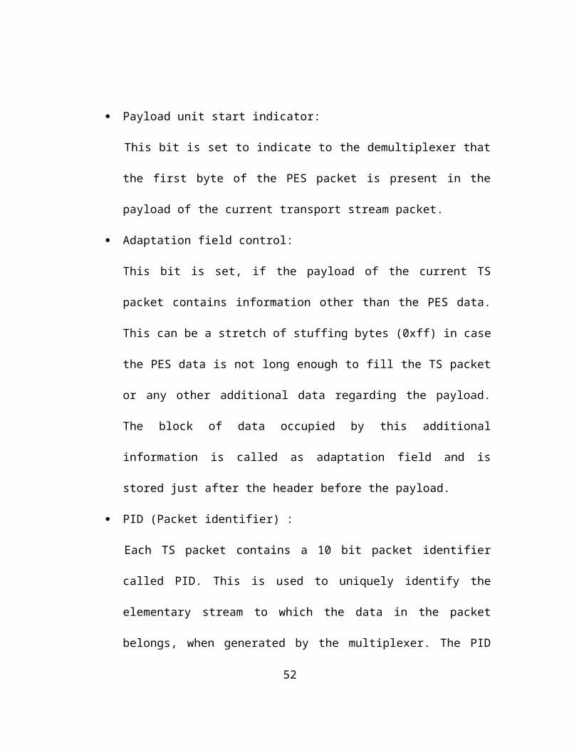
APPENDIX A

Multiplexing – Matlab source code

clear all

clc

global Aframe_number_reset;

global Vframe_number_reset;

global Alocation;

global Aframelength;

global Vlocation;

global VPES;

global APES;

global n;

global q;

global p;

global V;

global A;

global vid;

global aud;

audio = input('Enter the name of the aac file with extension','s');

57

video = input('Enter the name of the 264 video file with extension','s');

fps = input('Enter the frames per second of the video');

fid = fopen(audio);

A = fread(fid);

m=0;

i=1;

while (i<length(A))

temp1 = dec2bin(A(i),8);

temp2 = dec2bin(A(i+1),8);

Asyncword = bin2dec(strcat( temp1,temp2(1:4)));

zero_bits = bin2dec(temp2(6:7));

if (Asyncword == 4095 && zero_bits ==0)

m=m+1;

temp = dec2bin(A(i+3:i+5),8);

Aframelength(m) = bin2dec(strcat(temp(1,7:8),temp(2,:),temp(3,1:3)));

Alocation(m) = i;

i = (i + Aframelength(m));

else

i=i+1;

end

end

58

Alocation(m+1) = length(A)+1;

temp3 = dec2bin(A(Alocation(1)+2),8);

freq = bin2dec(temp3(3:6));

% frequency detection

freq_table=

[96000;88200;64000;48000;44100;32000;24000;22050;16000;12000;11025;8000];

if freq > (length(freq_table)-1)

disp('Unknown Audio Sampling Frequency Detected');

else

frequency = freq_table(freq+1);

Aframe_duration = 1024/frequency;

End

% reading video file

fid = fopen(video);

V = fread(fid);

m = 0;

for i = 1:length(V)

if ( V(i)==0 && V(i+1) ==0 && V(i+2) ==0 && V(i+3) == 1 )

m = m+1;

59

Vlocation(m) =i;

temp4 = dec2bin(V(i+4),8);

Vframetype(m,1) = bin2dec(temp4(1,5:8));

end

end

Vlocation(m+1) = length(V)+1;

Vframe_duration = 1/fps;

% starting the mux

%setting frame number reset

if Vframe_duration >Aframe_duration

Vframe_number_reset = 65535;

Aframe_number_reset = round(65535*Vframe_duration/Aframe_duration);

else

Aframe_number_reset = 65535;

Vframe_number_reset = round(65535*Aframe_duration/Vframe_duration);

end

global k;

k = 1;

n = 1;

q = 1;

60

p = 1;

Vmux_time =0;

Amux_time = 0;

Vcounter =0;

Acounter =0;

Vnext_begin = 1;

Anext_begin = 1;

A_done =0;

V_done = 0;

global name;

global TS_number;

name = [1:54000];

name = dec2bin(name);

TS_number =1;

Vid_PES();

Aud_PES();

while( A_done == 0 || V_done ==0 )

vmux_chk(TS_number) = Vmux_time;

amux_chk(TS_number) = Amux_time;

if (((Vmux_time < Amux_time) || A_done == 1) && V_done ==0)

61

PID = bin2dec('1111');

begin = Vnext_begin;

if begin ==1

VTS_num = ceil(length(VPES)/185);

VTS_size =1000*Vframe_duration/(VTS_num) ;

end

if length(VPES)>185

data = VPES(1:185);

Vnext_begin =0;

VPES = VPES(186:length(VPES));

else

data =VPES;

Vnext_begin = 1;

k = k+1;

if k<= length(Vlocation)-1

Vid_PES();

end

end

TS(PID,data,begin,Vcounter);

62

if Vcounter >=15

Vcounter =0;

else

Vcounter =Vcounter+1;

end

Vmux_time = Vmux_time+ VTS_size;

else

PID = bin2dec('1110');

begin = Anext_begin;

if begin ==1

ATS_num = ceil(length(APES)/185);

ATS_size =1000*Aframe_duration/ATS_num ;

end

if length(APES)>185

data = APES(1:185);

Anext_begin =0;

APES = APES(186:length(APES));

else

data =APES;

Anext_begin = 1;

n = n+1;

63

if n<=length(Alocation)-1

Aud_PES();

end

end

TS(PID,data,begin,Acounter);

if Acounter >= 15

Acounter =0;

else

Acounter =Acounter+1;

end

Amux_time = Amux_time+ ATS_size;

end

if (k>(length(Vlocation)-1) && Vnext_begin ==1)

V_done =1;

end

if (n>(length(Alocation)-1) && Anext_begin ==1)

A_done =1;

end

end

64

% PES header with first 3 bytes 0x000001, 8 bits - stream ID, 2 bytes of PES length

including header and 2bytes of frame number.

function Aud_PES()



global Aframelength;

global Alocation;

global Vlocation;

global VPES;

global APES;

global n;

global q;

global p;

global V;

global A;

global k;

global aud;

% constructing PES

65

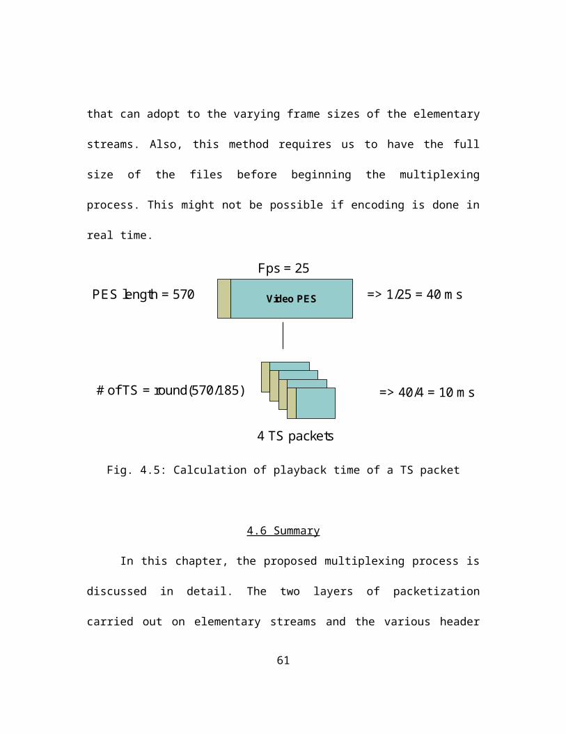
stream_id = bin2dec('11100000');

frame_length = Aframelength(n);

if p<=Aframe_number_reset

Aframe_number = p;

p=p+1;

else

Aframe_number = 1;

p=2;

end

bin_frame = dec2bin(Aframe_number,16);

Aframe_number_byte1 = bin2dec(bin_frame(1:8));

Aframe_number_byte2 = bin2dec(bin_frame(9:16));

Aframe_length= dec2bin((Aframe_length+8),16);

Aframe_length1 = bin2dec(Aframe_length(1:8));

Aframe_length2 = bin2dec(Aframe_length(9:16));

APES=

[0;0;1;stream_id;Aframe_length1;Aframe_length2;Aframe_number_byte1;Aframe_nu

mber_byte2;A(Alocation(n): Alocation(n+1)-1)];

aud(n) = Aframe_number;

66

function Vid_PES()



global Alocation;

global Vlocation;

global VPES;

global APES;

global n;

global q;

global p;

global V;

global A;

global k;

global vid;

% constructing PES

stream_id = bin2dec('11000000');

Vframe_length = Vlocation(k+1)-Vlocation(k);

if q<=Vframe_number_reset

Vframe_number = q;

q=q+1;

67

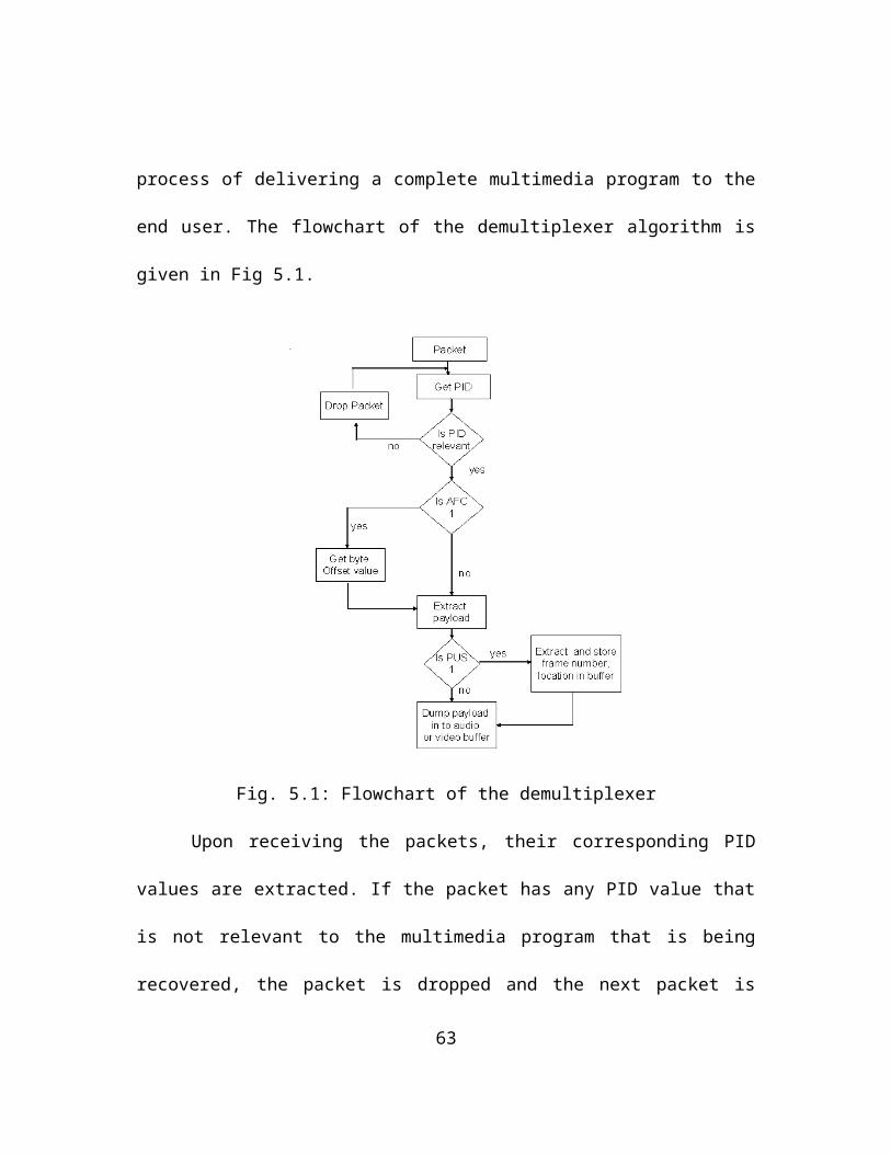
else

Vframe_number = 1;

q=2;

end

bin_frame = dec2bin(Vframe_number,16);

Vframe_number_byte1 = bin2dec(bin_frame(1:8));

Vframe_number_byte2 = bin2dec(bin_frame(9:16));

Vframe_length = dec2bin(Vframe_length+8,16);

Vframe_length1 = bin2dec(Vframe_length(1:8));

Vframe_length2 = bin2dec(Vframe_length(9:16));

VPES=

[0;0;1;stream_id;Vframe_length1;Vframe_length2;Vframe_number_byte1;Vframe_nu

mber_byte2;V(Vlocation(k): Vlocation(k+1)-1)];

vid(k) = Vframe_number;

function TS(PID,data,begin,cont_counter)

global TS_number;

global name;

TS_packet =zeros(1,188);

begin_frame = dec2bin(begin,1);

if length(data)<185

68

offset = 188-length(data);

adaptation_field ='1';

header=

strcat(begin_frame,adaptation_field,dec2bin(cont_counter,4),dec2bin(PID,10));

header1 = bin2dec(header(1:8));


TS_packet(1:4) = [71; header1;header2;offset];

TS_packet(offset+1:188) = data;

else

adaptation_field ='0';

header=

strcat(begin_frame,adaptation_field,dec2bin(cont_counter,4),dec2bin(PID,10));



TS_packet = [71;header1;header2;data];

end

filename = strcat(name(TS_number,:),'.bin');

fid = fopen(filename,'w');

fwrite(fid,TS_packet);

fclose(fid);

TS_number = TS_number+1;

69

APPENDIX B

Demultiplexing – C++ source code

#include <iostream>

#include <fstream>

#include<string.h>

#include<math.h>

using namespace std;

ifstream::pos_type size;

char *memblock;

char name[20];

void ret_str(char* s)

{

if(*s != '\0')

ret_str(s+1);

char *x = (s);

strncat(name,x,1);

}

70

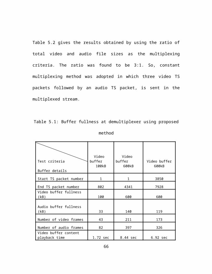
int main()

{

int framenumber;

int PES_length;

int streamid;

int payload_unit_start;

int adaptation_field;

int cont_counter;

int PID;

int offset;

int invalid_packet;

int vf = 0;

int af = 0;

int V[5000][3];

int A[5000][3];

int *Video;

int *Audio;

Video = new int [10000000];

Audio = new int [10000000];

int *Vend;

Vend =Video;

71

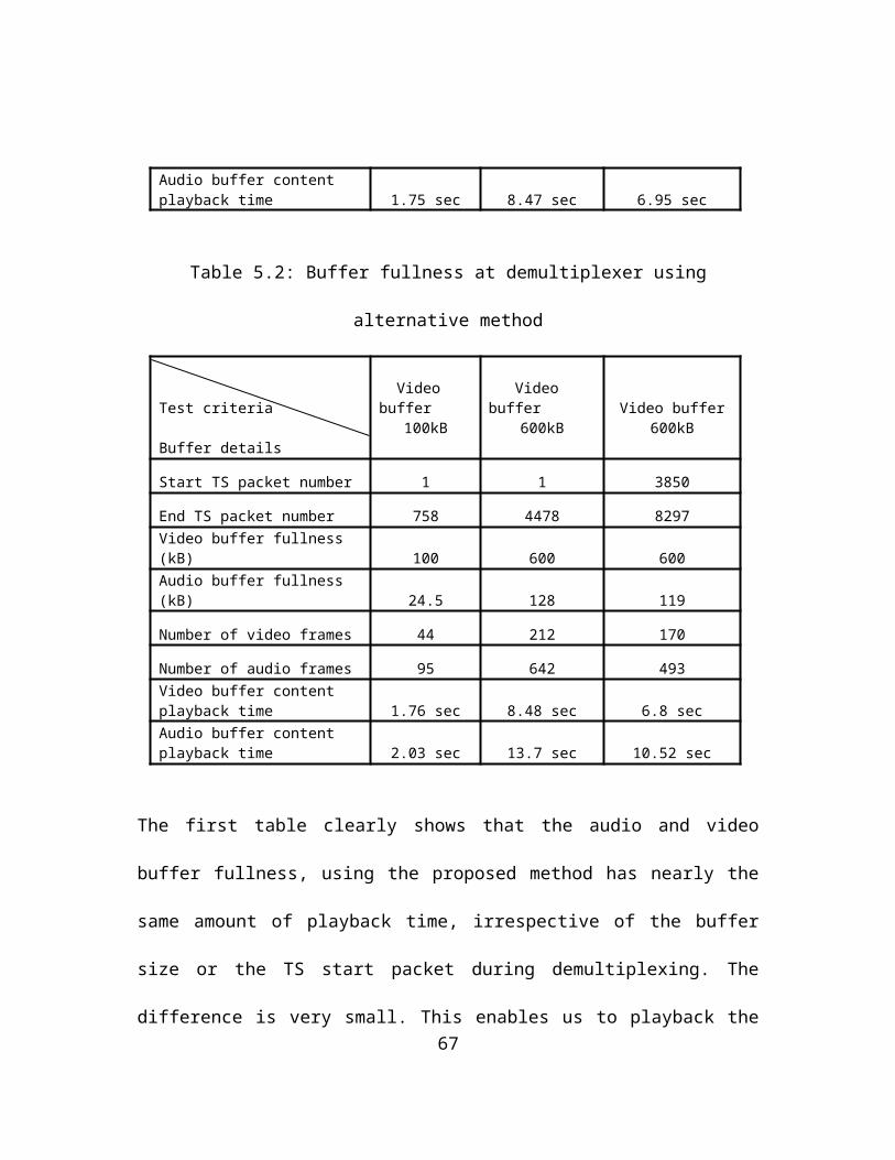
int *Aend;

Aend=Audio;

int remainder;

char a[16],b[16];

strcpy( b,"0000000000000000");

int ts;

cout<<"Enter the packet number you want to start with";

cin>>ts;

for(int num = ts;num<54999;num++)

{

strcpy(a,"");

int number = num;

int i = 0;

while(number > 1)

{

remainder = number%2;

if (remainder==0)

strcat(a,"0");

else

strcat(a,"1");

number = number>>1;

72

i++;

}

strcat(a,"1");

strncat(a,b,(15-i));

strcpy(name,"");

ret_str(a);

strcat(name,".bin");

ifstream file(name,ios::in|ios::binary|ios::ate);

if (file.is_open())

{

size = file.tellg();

memblock = new char [size];

file.seekg(0,ios::beg);

file.read(memblock,size);

file.close();

}

else cout << "unable to open";

unsigned char k = *memblock;

if (int(k) == 71)

{

73

invalid_packet =0;

k =*(memblock+1);

payload_unit_start = ((k>>7)&0x1);

adaptation_field = ((k>>6)&0x1) ;

cont_counter = (k>>2)&0xf;

unsigned char l = *(memblock+2);

PID = ((k&0x3)<<10)|l;

if (adaptation_field ==1)

{

k =*(memblock+3);

offset = int(k);

memblock =memblock+offset;

}

else

{

offset = 3;

memblock =memblock+3;

}

}

else

{

74

invalid_packet =1;

cout<<'\n'<< " Invalid paket Received";

}

if (payload_unit_start ==1)

{

if ( (*(memblock)==0) & (*(memblock+1)==0) & (*(memblock+2)==1))

{

k = *(memblock+3);

streamid = int(k);

k = *(memblock+4);

unsigned char l = *(memblock+5);

PES_length = (k<<8|l);

k = *(memblock+6);

l = *(memblock+7);

framenumber = (k<<8|l);

memblock =memblock+8;

offset = offset+8;

}

else

{

invalid_packet =1;

75

cout<<'\n'<<"Packet error : no PES header";

}

}

if (PID == 15)

{


{

if (vf==500)

{

float temp,temp1;

int Iframe =0;

int aframe =0;

int n = 0;

int m = 0;

int p =0;

int vfnum;

int afnum;

do

{

int y = *(Video+V[n][2]+4);

p = y&0x7;

76

if(p == 0x5)

{

vfnum = V[n][1];

temp1 = vfnum;

temp = (48000*(temp1-3)/(1024*25))+1;

afnum = temp;

if( (temp-afnum)>0.5)

afnum =ceil(temp);

else

afnum=floor(temp);

for(int y=0;y<af;y++)

{

if(A[y][1] == afnum)

{

Iframe =1;

m = y;

y = af;

}

}

}

77

else cout<<"";

n++;

}while(Iframe ==0);

n--;

int vdata = V[vf-1][2]-V[n][2];

int adata = A[af-1][2]-A[m][2];

ofstream vid;

ofstream aud;

ifstream z;

char *zbuff;

zbuff = new char [21];

z.open("z.bin");

z.seekg(0,ios::beg);

z.read(zbuff,21);

z.close();

remove("new_video.264");

remove("new_audio.aac");

vid.open("new_video.264");

aud.open("new_audio.aac");

if (Iframe ==1)

{

78

for (int i =0; i<21;i++)

{

unsigned char h = *zbuff;

vid<<h;

zbuff++;

}

for ( int i =0; i<vdata; i++)

{

vid<< char(*( Video +i+V[n][2]));

}

vid.close();

for (int i =0; i<adata; i++)

{

aud<< char (*(Audio +i+A[m][2]));

}

aud.close();

}

cout<< "\n one block";

system( " ./test.bat ");

vf =0;

79

af =0;

Vend =Video;

Aend =Audio;

}

V[vf][0]=PES_length-8;

V[vf][1]=framenumber;

V[vf][2]=(Vend-Video);

vf++;

}

for (int i = 1;i<=(188-offset);i++)

{

k = *memblock;

*Vend = int(k);

memblock++;

Vend++;

}

}

else if (PID == 14)

{


{

80

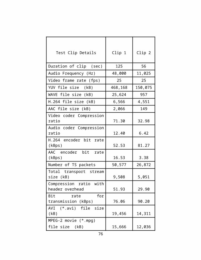
A[af][0]=PES_length-8;

A[af][1]=framenumber;

A[af][2]=(Aend-Audio);

af++;

}

for (int i = 1;i<=(188-offset);i++)

{

k = *memblock;

*Aend = int(k);

memblock++;

Aend++;

}

}

}

cout<<'\n'<<"Done";

return 0;

}

81

Documents

University of Texas at Arlington Dissertation Template · Web viewThis is taken into account during the multiplexing process as explained in section 4.4. Table 5.1 gives the details