UNIVERSITY OF SASKATCHEWAN

This volume is the property of the University. ' Saskatchewan, and the literaryrights of the au thor and of the Uni versi ty must be respected, I. :'he reader ob­tai ns any assi stance from thi s volume, he must gi ve proper credi tin hi s own work.

This Thesis b)~ . )a.m~s Horojd, T90 pe , , , " e , • , ., , •• • • • " • "

has been used by the following persons, whose signatures attest their acceptanceof the above restri cti ons .

Name and Address Date

APPROXI~~TIONS BY I~ANS OF CONTINUED FRACTIONS

A Thesis

Submitted to the Faculty of ~raduate Studies

in Partial Fulfilment of the Requirements

for the Degree of

r..Jaster of Arts

in the Department of Mathematics

University of Saskatchewan

by

James Harold Toope

Written under the Supervision of

Professor N. Shklov

Saskatoon, Saskatchewan

f

". _.. };;_~::,_i

March, 1960

The University of Saskatchewan claims copyright inconjunction with the author. Use shall not be made ofthe material contained herein without proper acknowledgement.

d 1 9 1952

UNrVER5I'f¥· OF ~SA:BKATCnEWA.N,

·'Departm~:o.t·q~'l1~tXJ.ematies:·

?:!fll}~.'.jra~u1t"~· ••Of·••;;.~.ra.dllat~··· •••• ;$.tudi.e's',·:.t.:rI1;1~ er~:~i~y·.·.~:r:: Saskat~hE)wan.· '. '".

fW.rJ\·:.t!t~.••·.,.· .•lIie~lb.~rs·· •.~or·····.the.· •..·C<5m!li.'~.te·e< .••aPt>Oin"te.d···.·••.•to·•.,;e~~lne~1tllE(,~~"~j.$},~;Rb~~~·$~·~: •·.·.. by- ·James." Ha!!0J..c1.·..•·Toope, ." .]3-~~'. ". {S aslt'.),\· .,··~·11·,fI.a~t1a:r.;.~~lr~.:t1ll~:at.of· the .reqUiremen'tS,fo:r"tn~Dt'.•~.·•.·•..:ge..rtlff';~[i~·~#;s~e~~jS~:t.Ar~ts.," "beg.:\;o·'.re;PQ;rt tl1a.t we eonsid:er' 14

·tti"ej~l$.!:sa:tls!:ac'tory< ~9'tP'tlJ.·f'9.r:Ql <¥1d'eonten'b'~' '

·~·fgtt~J:I(re·<Qt.•.• ~he$l·s.·.: ,:}.A;P':p·t·Q~~1'l1ati.oI1.s ..• '.• by.Means .ot"Qont:tnu.ed::J'ra~t;on$.·

···lfe.···:~l·~·;~+'$llo.~~ .•·.•·~t~a.t···.MI(~ ..~8p.p.e.··'lla·s··.·· •••.~lle.e ..f3..s~ilt· ••••••~pa.s ~~d.""'an.: ora.~pexalli~+lat~lf.'l;lO:p..···'b~~.,·g.~e~al.• ~fle'l.~,.·of .••. tn.~.>'\tb j"ect>so~ihis .thes-i.$.. . . .. . '

~pr()f.$6,SO

r'~~~$'slill- ·;;·-"-, to' '---~:-;71', ,"--',' '''''"-'1' " -_":,J:<>~'_ " --~--":,:-:' ,:- . - ','i, " • ,"<' -_.~,;, -<~,>::;i~~-:'c,:

iii

I wish to express my sincere thanks to Professor

N. Shklov for directing this study. His unfailing

kindness and ever-ready assistance are deeply appreciated.

The staff of the University Library spared neither

time nor effort in making books available.

To my wife Dorothy special thanks are due for

assistance in typing the manuscript. The tedious work

of penning in superscripts, subscripts, symbols and

correcting errors was also hers.

iv

TABLE OF COr~TENTS

Chapter Page

o. INTRODUCTION. • • • • • • • • • • • 1

I. HISTORICAL DEVELOPMENT • • • • • • • • • 3

II. THE CLASSICAL THEORY OF CONTINUED FRACTIONS

III. THE ANALYTIC THEORY OF CONTINUED FRACTIONS •

• • 10

• • 42

IV. REQUIREI\t1ENTS FOR COMPUTER APPLICATIONS •

v• CONTINUED-FRACTION EXPANSION OF FUNCTIONS

t • • 63

• • • 79

VI. CONVERGENCE OF FRACTIONS TRANSFORJ.\1ED FROlvlSERIES. • • • • • • • • • • • • • 94

VII. CONVERGENCE OF CONTINUED FRACTIONS FORlvIEDFROM: INVERTED DIVIDED DIFFERENCES. • • • • 122

VIII. CONCLUSION • • • • • • • • • • • • • 126

APPENDIX • • • • • • • • • • • • • • 128

t\TORKS CITED • • • • • • • • • • • • • 132

v

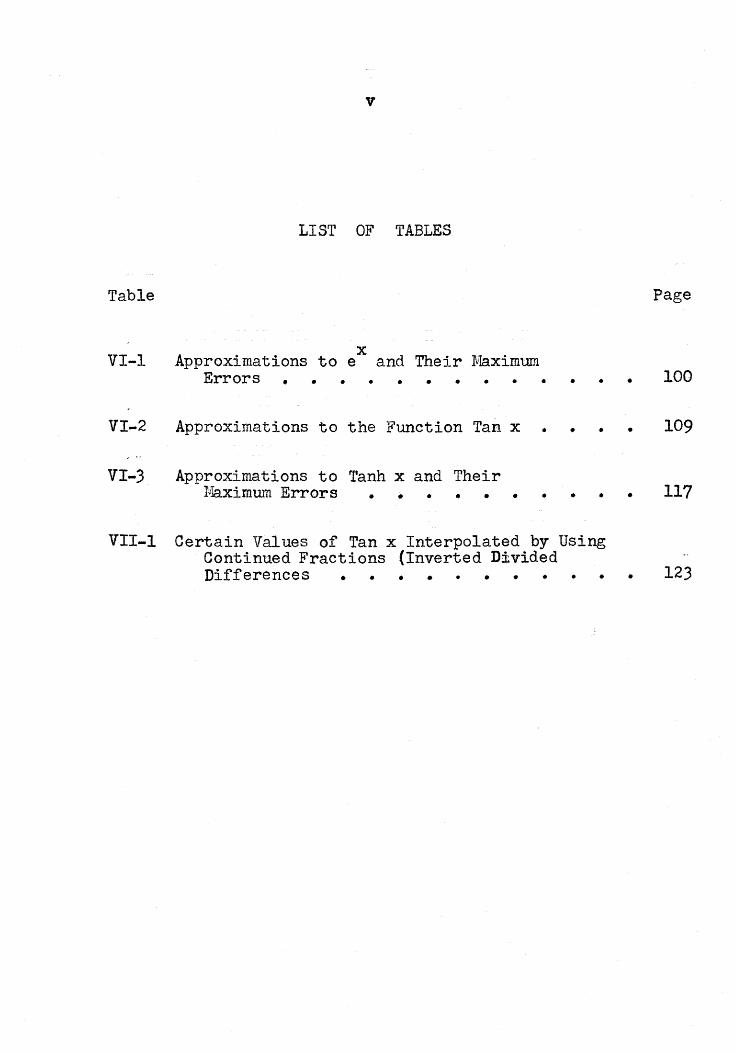
LIST OF TABLES

Table Page

100••••• • • • ••

xApproximations to e and Their ~~ximum

Errors • • •VI-l

VI-2 Approximations to the Function Tan x • • • • 109

VI-3 Approximations to Tanh x and Theirp~ximmn Errors • • • • • • • • • • 117

VlI-1 Certain Values of Tan x Interpolated by UsingContinued Fractions (Inverted DividedDifferences • • • • • • • • • • • 123

vi

LIST OF FIGURES

Figure Page

IV-l Functional Relations of a Computer • • • • 67

V-l Calculation of Cot 0.15 Using Divided­Difference Continued Fractions • • • • 90

VI-1 Graphs of eX and Some of its Approximants • • 97

VI-2 Graph of One Branch of Tan x and its FirstThree Approximants • • • • • • • • 105

VI-3 Graph of Tanh xApproximants

and its First Three• • • • • • • • • • 114

o.

1

INTRODUCTION

Rational approximations to real numbers have been used

from ancient times, either for convenience in computation, or

due to lack of more precise knowledge of the magnitude of the

numbers. Better approximations may be obtained by making

corrections in the form of adding aliquots, adjusting

numerators, or adjusting denominators. The latter method,

when extended, leads to our modern notion of continued

fractions.

The classical theory of continued fractions began during

the Renaissance when Arabie numerals and the modern fractional

notation had become common.. It was studied and extended until

about the end of the nineteenth century. This theory is

concerned with terminating or non-terminating continued

fractions whose elements are integers. 'flhe classical theory

is essentially complete, beinglf11sed,'.mafutrl' as a tool in other

investigations, chiefly the solution of Diophantine equations.

Advances are announced from time to time in special areas

of the field.

The equivalence of continued,fractions to infinite

products and to series expansions was recognised early in

their study. Series expansions proved most convenient at

that time, the other two forms being relatively .neglected

until more powerful computing aids were developed.

2

Modern function theory regards the elements of a

continued fraction as variables or as functions of variables.

This analytic theory of continued fractions resulted from

developments in the evaluation of integral functions,

polynomial interpolation, rational functions and similar

problems. This study has developed rapidly during the past

sixty years and much research continues to be done.

The development during the past decade of programmed

electronic digital computers having great speed and freedom

from error has stimulated the development of new numerical

methods and a reexamination of old methods of computation

for computer use. Tn particular the ability of the digital

computer to iterate a series of operations ("loop") has

stimulated the search for algorithms that may be used to

evaluate functions. One such algorithm is the continued

fraction.

It is the purpose of this thesis to examine the method

of evaluating functions as continued fractions with a view

to its adaptability to computer operations.

I

3

HISTORICAL DEVELOPF~NT

The continued fraction is a comparatzvely modern devel­

opment in mathematics, having been studied intensively only

since the Renaissance. The ancient Greeks may have had an

inkling of continued-fraction operations, but a poor notation

hampered their manipulation. Some of their geometric results

suggest continued-fraction operations, but these are likely

the expression of parallels between geometric and algebraic

operations. Archimedes gave for j3: the approximations

i~§ < jT < 1,~

which are the 9t h and 12t h approximants (convergents) of the

simple continued-fraction expansion of [3. Dantzig [5]surmises that this result was obtained using Hero's geom-

etric approximation to a square root, which resembles the

modern Newton-Raphson method of approximation. A value of

5/3 apparently was used as the initial approximation, but

no reason was given for this choice.

Another Greek development, the Euclidean algorithm,

seems to have suggested the continued-fraction expansion of

rational numbers and this was rapidly formulated using

Arabic numerals and modern fractional notation follo\rlng

the Renaissance. Thus Euclid's algorithm for the H. C. F.

of two numbers a and b may be written

etc. ,,

,

q +..1 =:1 r

o

...!.. :: q +. r o

bOb

b

to give the simple continued fraction development'

alb = q 0 + .' .J. ,ql+_1......., _

, qz + ••

•'1

q +1""-1------q"" ,

where the process terminates when r",:'0, for a and b integers.

Raffaele Bombelli [13], around 1572, used non-terminating

continued fractions to approximate square roots in the form~

Vai+b= a"'~b ____-2a of- b

-e;;.-.---~a ....

• .,

••

His method of deriving this result seem obscure, but I suspect

he used the following method based on completing the square.

Thus the equationz

x - 2ax-b:: 0 1

has the positive root

5

(where early mathematicians tended to ignore the smaller

root) and the equation may be written in the alternate form

x =2a + b/x •

Combining these results we have

j a' + b : x - a =x +- b/x •

As the value of x is substituted successively the infinite

continued-fraction form is generated.

Pietro Cataldi, about 1613, originated the modern

continued-fraction notation and developed some theory for

the form having integral elements. Bartolotti claims that

C~taldi discovered the recurrence relation of approximants,

estimates on the size of error involved in using approxim-

ants and the fact that successive approximants of proper

continued fractions are alternately in excess and in defect

of the value generating the continued fraction.

These latter results seem to have been discovered and

used by John Wallis and Christian Huygens at about the same

time. The classical theory of continued fractions was devel-

oped, and rigorous proofs of the properties given, by Euler

and Lagrange [5J. Extensions were made to this theory by

Legendre, Gauss, Jacobi, Galois, Liouville and others. These

savants were interested in the properties of approximants

mainly as tools in solVing problems in number theory.

6

This' classical theory (mainly concerned \tlith forms having

integral elements) concentrated on the expansion of quadratic

surds, these being most useful in number theory. For instance

the expansion' V2 = 1 +_1_2+1

2+.•

•

is easily obtained by noting that

12= 1 + fi -1 =1 + 1· = 1'" 117(\fE -1) --='12=-+-1-

and usingfi+1 -= 2+ 1

v'Z+1

The form is a simple continued fraction (having partial

numerators alII) and the partial denominators repeat.

This latter is a characteristic property of the simple continued­

fraction expansion of a quadratic surd, where after some stage

'.'the denominators repeat in blocks (cycles)_ In this example

the cycle has length one_

William Viscount Brouncker, the first president of the

Royal Society [ 1+J, did much work on the continued-fraction

expansion of quadratic surds, as well as the expansion of some

other irrational numbers such as

- ,which he derived from Wallis' infinite product

1+ 3-3-5-5-7-7-9-9-11-11- •••1T::' i -1+.1+.6 -6. 8-8.10.10.. • • _

7

There seems to be no record of his method.

Lord Brouncker also used continued fractions to give the

first systematic solution, in 1657, to Pell's equation

x~- Ny2= 1, or x~- Ny~= -1.

(The equation was wrongly ascribed to Pe1l by Euler.)

Euler's "De Fractionibus Continuo", in 1737, extended

previous ~ork to give a comprehensive classical theory as of

that time. Thereafter this classical theory was used mainly

as a tool in number theory, particularly for the solution of

Diophantine equations. Liouville [12J used continued fractions

to give the first proof of the existence of transcendental

numbers.

Infinite series, infinite products and continued fractions

originated and were studied at about the Same time. Methods of

conversion from one of these forms to another ~~re worked out,

at least for special cases. This suggested that functions could

be represented as continued fractions whose elements are

variables (or functions of other variables). The continued-

fraction forms were of less practical use than series and the

analytic study lay dormant until the latter part of the

nineteenth century.

T. J. Stieltjes I14J began the modern analytic study when

he investigated the continued-fraction expansion of aSymptotic

series representing definite integrals of the form

f(u) duZ+U

, f(u» 0 •

The form of continued fraction he obtained is known as an

S-fraction or StieltjeB~fraction, and certain restrictions

are placed on the elements.

In 1903 E. B. Van Vleck [15J began the eXbansion of

Stieltjes~ theory by transforming the fraction form and

relaxing some of the restrictions on the elements. Hamburger [ 8Jcompleted this extension by 1920. Several mathematicians of the

same period connected the ideas of infinite continued fractions

with Hilbert's conception of infinite matrices and quadratic

forms having infinitely many variables. Independent workers in

this field were Hellinger (who developed a complete theory by

1922), Carleman,Nevanlinna, and Riesz.

Continued fractions having complex elements were investigated

by mid-nineteenth century when J. Worpitzky, in 1865, published

some convergence theorems. Further investigations were

undertaken by von Koch, Van Vleck, Szasz and others in the

first quarter of the twentieth century. The methods and results

were not closely related nor did they indicate a unified

theory or approach.

H. S. Wall and his associates approached the problem by

regarding the continued fraction as a product of linear

fractional transformations. 'Their results, published by

'Viall [17J in book form in 1948, contain many convergence

theorems. Some of these reduce to one or more previous theorems

as special cases, others are entirely new. Stieltje 5." fraction

is treated as a speCial form of a general type. The analogue

to an infinite matrix becomes another special form.

9

In general their theory has largely unified previous work on

continued fractions having complex elements.

In recent years some other forms of continued fractions

have been investigated. For example, Adam Puig [llJ has

investigated properties of continued fractions whose elements

are differentials. Anunoy Chatterjee [3J has extended his

investigation to continued fractions whose elements are

themselves continued fractions.

The utilization of continued fractions as a means of

evaluating functions on a computer has been s~ggested before

and I suspect has been carried out in one form or another,

but I have not been able to find any papers or books on this

phase of the subject.

- 0 -

10

II THE CLASSICAL THEORY OF CONTINUED FRACTIONS

1. Definitions and Notation

By a continued fraction we shall mean a fraction having

the form:

F = bo + at-.~-

bi + ~a--,L~_b'2, +a

3

b 3 + •

•

where we may regard the sign as belonging to the ai.

Other notations in use are:

(II-I)

· . . , (11-2 )

• • • , (I1-3)

• • • or (11,.4)'

(1I-5)

The ai/bi are partial Quotients,

the ai partial numerators,

the bi partial denominators

and the ai, bi are separately known as elements.

The complete denominator wn of the n th stage is the

value of the balance of the continued fraction beginning with

bn • Thus

11

The fraction obtained by stopping at the n th partial

quotient is called the n th approximant or convergent and

denoted by An/Bn,where

A~ is the n th namerator. and

Bn is the n th denominator.

Since any fraction is unaltered if we multiply numerator

and denominator by the same quantity cia, it follows that the

continued fraction is unaltered if we multiply af'l' b" and a"'+l

by c;i o. Any partial numerator or partial denominator may be

made positive and any negative sign included with the other

element by using e :.-1. Similarly, appropriate choices of c ' s

may be used to make al.L partial numerators ones or all

partial denominators ones.

Simple (or regular) continued fractions have each

partial numerator unity.

Proper continued fractions have each partial quotient

a proper fraction, that is ai"~ bi •

Finite (or terminating) continued fractions have only

a finite number of partial quotients.

Infinite (or non-terminating) continued fractions have

an infinite number of partial quotients, which mayor may not

be formed by a particular rule.

Recurring (or periodic) continued fractions have partial

quotients which repeat in blocks. The repeating elements form

the recurring period or cycle. Non-repeating elements, if any,

12

at the beginning form the acyclic part. The cycle is

denoted by asterisks thus

1 +;-.16 = 3 + 2 :: 3+ 1

4 2+

1- #

4

Finite symmetric continued fractions have equal partial

quotients equidistant from the ends of the fraction. A

recurring period or cycle "'Thich has this property is a

symmetric cycle or sym~etric period.

Convergence. A continued fraction converges, or is

convergent, if the sequence of approximants (convergents)

tends to a finite limit and consequently if at most only a

finite number of denominators vanish. If convergent, its value

is defined to be the limit of its approximants. Otherwise

it is divergent or OSCillatory according as the sequence

diverges or oscillates.

Uniform convergence. If the elements of a continued

fraction are functions of one or more variables over a given

domain D, if the fraction converges for all values of the

variable or variables over D and if the sequence of

approximants converges uniformly over D, then the fraction

converges uniformly over D.

Convergence set. If a continued fraction converges when

all its elements are contained in a set of points D in the

complex plane, this set D is a convergence set for the fraction.

Convergence sets have been found for special forms of

13

continued fraction, such as the form having all bi ::: 1.

The~ part of a given continued fraction is a new

continued fraction whose approximants are the same as the

even approximants of the given continued fraction.

Similarly, the odd part of a given continued fraction

is a new continued fraction whose approximants are the odd

approximants of the given continued fraction.

2. Relations Among the Approximants

A recurrence relation between succeeding approximants is

easily established by induction.

Proof.

The relation is

(II-6)

We 'note Ao bo-=-,s, 1.

Al =b l bo + a 1 ,

B1 bI

Ab .t (b.1 b, + a 1) + a;z. b 0#_2. ::: -=- _

B2,. bz b1 + at.1

and so the relatiop holds for n =2. Now assume it holds

~rorlf<.k,-:soJthat',

,=--------

then by definition we form the k th approximant by replacing

b/<"1 by bl<-l + a 1(' to getb~

A/( _ (bk _1+ ak/b I< ) (1/(-1) + a tc-zAk _.1

Bk (b lt - l + al</bl( ) (B,,-.l) ..... a/(-lB 1<-3

14

b , (b"'-lAI(_z.+ a k - 1AI< _J) + akA",_t..

-=bl( (bk - 1B R- 1+ ak-.tBko,) + a"BI<_1.

bI<AI<_l+ aI(AI<_z.

bI(Bk - t "" aItBj(-", as was to be shown.

We note that if in (II-6) we replace the n th partial

denominator b h by the n th complete denominator wn , where

b"+l + b,,+-1. +

• • • . ,

then Ah/B~ becomes the value of the continued fraction.

Using the recurrence relations, we may derive other

relations among the convergents, the most useful being the

determinant relations

B"_l

At,=(-If a Oa 1a1..

B"n=l,2,3, ••• , (11-7)

Bh

n=1,2,3, ••• , (II-B)

and in general

AIt _, Alii-I(+at'\

B"_J B,....

A,,_,.,

B",-1. {n=1,2,3,

k=l,2,3,

• •

• •

. ,

.n.(II-9)

This general case follows easily by writing

lA••• A.,. A"'_I< bnA.... / + a.,A k _ 1.

=E".I( B", B,,_~ s.a., + a.,B h _ "

s.: s.: A... 14. A",.1.=b., +a h •

E"'-H B",., B"_II( s..,(I1-7) follows from (11-9) with k =1 and repeated application

of the relation to the right hand side, where we define a, =-1.

15

n-=1,2,3, ••••

n :::.1,2,3, ••• ,

(11-8) :follows from (11-9) with k = 2.

Division of (11-7) by BI'H. B~ and (II-!) by Bft _1. Bl'l

yields the forms

A't/-l A", (-1 f' a 1 a%,. • .a "I--- =BII . ! Btl B", B"'.IA.... ,. All (-lf~Jala1. ••a"_1b",---- = ,

(11-10)

(II-II)

Again, using the recurrence formulae (II-6) in the form

b , +

B" b +--= "B"~l

we see that

,

, n ::= k , k-1, • • .3,2.,

(11-12)

,• • •

b lot - l + b "-1 ....

BII b, + a", att.-J a, a1"::: ---_ ... -.

3. Proper Continued Fractions [10]

Thus far in our definitions and relations we have

restricted our elements only to those obeying the operations

permitted in a field. We shall now restrict our elements to

the real numbers and take any arbitrary sequence of positive

integers fai } for our partial numerators. We now expand any

real numblr Yo by taking bo to be the largest integer in Y6 ,

b(J =[ YoJ ' and using

16

(II-13 )•,a~

Y - b_- J.,..-1 ..r. =----

We obtain the expansion

• • • a" ...,b,,+

(II-14)

where b o may be either positive or negative and, by the

contruction (II-13), bn~ a~ for n : 1, 2, •• • Hence each

partial quotient is a proper fraction. We now have

Theorem II-I.

Yo is rational if and only if its expansion as a

proper continued fraction terminates.

Proof.

If the proper continued-fraction expansion terminates,

it,must represent a rational number.

It remains to show that if Yo is rational its expansion

terminates. Put (II-13) in the form Y"'~I - b",,,, =a.,..jy-x •

If Yo is integral this proves the theorem. If Yo is rational,

say Yo = Ptl /qo' (Po' qo)' =1, expansion by the algorithm

shows that each succeeding ~ must be rational. If the

expansion is to terminate some ~ must be integral. Let

p. ,q.> 0,I. (,

so that

q . - p - b q.l- - i-I i_,e.-/

Hence 0< p b q < qi-I - L'-/ . i.-I . I>' ,

which must be true for all i when Yi is non-integral. But

this says that the denominators qi of the y~ have the relation

17

a descending sequence of positive integers. Hence some

q~ =1, y~ is an integer, and the algorithm must end,

as was to be shown,q.e.d.

The following theorem holds for an infinite proper

continued fraction.

Theorem II-2.

Every infinite proper continued fraction converges

to the number which generated it.

Proof.

Since , (I1-15)

A-II-z Y"fI. (A"'~IB~~~ - A"~2.B"J1_' )Yo - "lr:':'; ~ B~~z (y?\ B"'_l + a.,.B 71-Z )

= (-If{ a, at~~_: .a.-z 1{B~~ + ~~~Jy~ )B~-z 1· (II-16)

The first term of the product on the right-hand side is in

absolute value less than 1, since B",,_7. =b I b~. • •b ... _t pl.ua

other positive terms and b.~ a·. The second term tends to,j J

Hencezero for the aj bounded or unbounded.

zero as n increases without bound, since a"., /B"tt_1 tends toA")\-2

Yo -:s::tends to zero for n increasing without bound,

q.e.d.

The change in sign in equation (T1-16) shows

Corollary·rT-l.

The even approximants are less than Yo.

The odd approximants are greater than y •o

18

By our restrictions on the elements and from the

recursion formulae (I1-6), we see that both the numerators

and the denominators form monotonic increasing sequences

. . . ,Ao<A1<Al.<AJ < •

,Bo< B]<B1.<B 3 < •

This fact \~ use to prove

• •

Theorem 11-3.

Each approximant is a closer approximation to Yo than

its predecessor.

Proof.

Solving (1I-15) for Y" , we have

Yo B....] -A tl • 1 =- ;,," (~ Bh.'L - AI\.2.) , or

y.. - A"-1 _ .... aft.B.... '" (~ - Ah _1 ! BI'I -l ) ,o B-1" BlI"~

".~

which is the statement of our theorem, since a~/~Ll by

construction, and BVi_",!B.. _:J. L...l, by our previous remark.

We observe that, given any real Yo and a sequence of

positive integers {ail, the expansion of s; as a proper

continued fraction is unique. For suppose it were not, e.g.

• • •

d + d +1 1.

. . . ,

then bo =do by construction, and

whereY1 = b.1 + a.t ••• , and Zl = d1 + a 1. •••

b, + d ; +Hence b i ~ d 1 , and we complete the proof by induction.

19

For a terminating proper continued fraction we specify

that bl(> al( for the last partial quotient, since if b,,= a1('

aK/b~=l, and we could terminate the expansion with the partial

quotient a t - 1/ (b k - s + 1) • Conversely, if the'l'a.st '~,bk .,is not

t(r~be::restrtct.ed·1- bl( > ale, we may have two expansions for any

given rational, differing only in their ultimate and penultimate

partial quotients in the manner shown.

Convergence of a proper continued fraction may be speeded

by proper choice of the {ail- In particular, every proper

continued fraction converges more rapidly than a geometric

series with ratio of 1/2. To see this we write

Therefore... ,- -- =- ------...

,

may be made arbitrarily

~ = ~ + (:: - ~) +(i-::)+. - • -

~ =~+lBh"1:: 1 < 1

6 " B,,+1. l-+b"+lB" 1 + all

a,...~ B"-1by using the recurrence relation, and

and b~~a~_ Hence our ratio6..h+~'"

small by choice of a h •

4. Simple Continued Fractions

Euclid's algorithm allows us to expand a rational fraction

into a continued fraction whose partial'numerators are all

unity. This simple, or regular, continued fraction is a special~,~~-::.~~..

(~\~I:R:':~ r:~~~!5ATCH~~

~------

20

case of the proper continued fraction, so we know th~se facts

a) Any real number may be expanded as a simple continued

fraction.

b) !his expansion is unique, except that a terminating

continued fraction may be arranged to have either an even or

an odd number of partial quotients by writing the last partial

quotient in either of the equivalent forms

at< a K

bi( - (b, -1) + 1/1•

c) A terminating simple continued fraction is the

expansion of a rational number and conversely.

d) An infinite simple continued fraction is the expansion

of an irrational number and conversely.

e) The even approximants are less than the value of the

fraction, the odd approximants are greater and each

approximant is a closer approximation than its predecessor.

The form of the simple continued fraction gives its

approximants special properties. From the determinant

formula (11-7) we have

A"B"_1 - Ah _ 1 Btl:: (-1r: , (II-11)

so that every approximant is in its lowest terms; further

A.. is prime to A~_1' and Btl is prime to .8,,-1_

The forms (II-10J and (II-II) simplify into

A.. · A"_1

{-1 r-:a.- - - - and (11-18)BII B"~1 B,,~J. s,

- - ----- =:----B,. B~.l

,

21

(11-19)

while (11-12) take; on the useful forms

Aft b_ -+ 1 1 1= • • •--+ - +"""5:"" ,A"'_1 b "-1 b, .•

B.. b" + 1 1(II-20)

• • • •=B... -:J, b)a-l+ b 1

We al-sohave- the fbllowi ng

Theorem II-Ir.

Any approximant A~/Bft of a simple continued fraction

is a closer approximation to the value of the fraction than

any rational fraction rls whose denominator is less than Bite

Proof.

We assume that s<:B .. and that rls is a closer

approximation to the fraction than either A~_]/B"_2 or A... /B ....

Thus r/s must lie between A.. /B.,. and A"-t/B,,.1.. Hence

Ir' A"_t A" A.... 2 1 1- - -- < - - - - ,so thats B..... 1 Bit B"-1 B"B"- 1

BoJrB•.• ., SAII•• /< s , where 1rB•. , - sAh-:a. is an integer.t"

Hence B"~s, which contradicts our assumption.

It is this property of the approximants of a simple

continued fraction which makes tham particularly useful for

numerical approximations. In the next section \"le s'I:iii-l

consider the maximum error involved in using an approximant

in place of the value of the fraction, also the problem of

22

tailoring an approximation to fit the conditions of a

particular problem.

All partial numerators are chosen to be I for the

simple continued fraction, so the fraction is completely

specified by the sequence of partial denominators. This

sequence is often referred to as the spectrum of the fraction

and the commonly-used notation is

y. =b0' bJ.' • • • • , b, and

• • • • ,ble" . . . ,for terminating and non-terminating forms respectively.

In the case of a periodic simple continued fraction, the

acyclic part (if any) is written before a semicolon, the

cyclic part is identified by writing one cycle behind the

,semicolon, ~!ith a bar above the cycle.

121=4; 1, 1,2,1,1, 8.

For instance

e =2; l, 2n, 1. , n=1,2,3, •••

The numerator Ah is a combination of be' ••b n , denoted

An -= [b 0' b l' • • • • bJ '

while the denominator B~is formed by the same rule from

b J , b1.' • • ,b t\ and is written

B, :: [bl' b 2. , • • • • b J .Euler f s rule [6J may be used to evaluate either

numerator or denominator from the spectrum, to evaluate

a partial denominator, or to evaluate a cycle. The rule

23

states

(1) take the product of all the terms,

(2) add all products formed when one pair of consecutive

terms is omitted,

(3) add all products formed when two separate pairs of

consecutive terms are omitted,

(4) add all products formed when three separate pairs of

consecutive terms are omitted, etc. ,

continuing until all possible products have been formed and

added. If n+l is even (an even number of terms in the

spectrum) we include the empty product (all terms omitted)

which we evaluate as :JJ~';.

The proof is by induction.

,cbolb1,bL ,

b. B.... +h_.l A

B"

A. = [b.] =b. ,

Al = [b o , b I ] = b. b l + 1,

AJ, = [b o , b] ,bJ :' b. b J b L + b. + b.. ,

~Here we note that

[bo ,b1 , • • • ,bh ]

or A" = b, + ,,-J A =Bl\ B..

where~_1A denotes the numerator of the complete quotient

following bo. Now if we assume Euler's rule holdS for the

right-hand side, then the right-hand term consists of that

part of the expansion of [bo,b 1 , •• ,b~] in which the pair

b"b1 is missing and the left term consists of the remainder

of the expansion of the left-hand side using Euler's rule.

24

As a corollary we note,that

[bo,b 1 , • • • ,b,,]": [b~, • '•• ,b 1,bo] .

The corresponding rule for the general form (II-l) is

obtained by transforming the latter into a simple continued

fraction and applying Euler's rule. The result is known

as the Euler-Minden relation.

5. Approximations Using the Approximant~

To determine limits on the error of an approximant

of a simple continued fraction we have

Theorem 11-5.

1 < 'b~+1. < E <_1_<1:....a, (B", + B"'+1) B"B"+ l B"B"+2 Btl

L, (1I-21)

whereE =

Proof.

We know A,,+1.' Yo, A",+s.---B~ ... 2. B..... 1

is either an increasing or a decreasing sequence, so

JA.' A,••<J A_, ' A, "+1

-" - -- < E <-:;::r -::-T 'B.. B,,+J. B". Btt • 1

whi ch ,~" DY':;:( IiI;;po:l R}'and:(:I I~:t9J'1: frltve~·~.]jh'e·~harr.ower·llfn).t s ,

The wider upper limit is obtained from B".1~B~. The

wider lower limit comes from the recursion formula (11-6)

written in the form

b".&

B"+1 + Btl ~B .. +% + B", •-"b..."

25

By similar reasoning we have thatcthe:cerror'tn'the ai-se

:of' 8.':;proper', continued'•. fr·actioIl') is

• (II-22)

These forms allow us to choose the most suitable

for

1 !I and we know Bn+:t= b"'+:tB~ + B"'-1.

this errorBt~·t~e error involved in using ~=~ and find that

for b\')+1 large, "\A'I'l/B'~3 .i~ an especially good approximation.1

This is also intuitively clear since for b~+1 large, b~+l

approximants for different applications. Thus the nth

approximantA~ of a simple continued fraction is in defectBh An even and in excess for n odd. The error in using ..•...~ is

13-;:We compareless than

is a particularly small change (correction) to b n •

Another application may require us to find the smallest

approximant having an error less than some arbitrary maximum

value l/a. In this case we calculate convergents until we

find one, A.,./B tI , such that BhBh+1~a. This is then the

required convergent. The condition is satisfied a fortiori

for B\,\~ va .In yet another case a problem may require an approximation

in a particular form for which no approximant is found suitable.

For example let us consider the problem [1 ] "given the length

of the mean solar year, f1nd.'a'conven:t:ent ··calenaar'e.orrec:bion~tt.v·a

26

The solution should be simple, easy to apply and have some

regularity in structure. In this case we proceed by takingI'

two convergents B~= andt: - one odd, one even -

and forming the fraction

p- =:

rnA. "", '·"·""""ntod+ ~v (11-23 )

Q mBod + nBev

where m and n are positive integers chosen to give a suitable

solution to the problem. It turns out that p/Q is a better

approximation than the earlier approximant and perhaps

better than the later approximant.

An important special case of this construction is that

of intermediate approximants or intermediate convergents.

Let A_/Bh be the nth approximant of a simple continued

fraction, and form the sequence

,

called the intermediate convergents between A~/~ and Ah"n./B",+2._

The r t h intermediate convergent is the r t h term follol"ling

An/Bnin the sequence. It uses the multiplier r and is

denoted p.. /0... •The intermediate convergents possess the following

properties, analogous to but differing from the properties

of the convergents themselves.

27

(a) The sequence is increasing or decreasing as A~, A~~~

belong to the increasing sequence of even approximants

or to the decreasing sequence of odd approximants.

(b) Every fraction PI" /0. to is in its Lowes t terms.

(c) Any fraction lying between P~/Qrand ~~l/Q~+lhas a

denominator greater than either Q~ or Qr+~

(d) Limits to the error in using Pr/Q.,. as an approximant

are given by•

and the

Properties (a), {b} and (c) are easily seen from the

relation ~+1 QI'" - p.. Q"+1 == A\,\+1:8", - A",Bt't+:L =(-1)'"

analogous properties for the convergents.

Property (d) follows since p~ ,cA~+1 , ~ ,1",+~- - -Q'" B",+1. :8"''''1

forms either an increasing or a decreasing sequence and if

r<b""''1.J

B.,.,.s Q ..

•

We may note in passing that any real number may be

expanded into a unique continued fraction for every sequence

of partial numerators that we may choose. The simple

continued fraction is then a special case where all the

partial numerators have been chosen as ones; cd.~:s·

approximants have been shown to, be in their lowest terms.

28

The approximants of a proper continued fraction are not

necessarily in their lowest terms and sometimes reduce to

an approximant of the corresponding simple continued fraction.

More generall~ the approximants of a proper continued fraction

are either reducible to an intermediate approximant or to

an approximation of the form p/Q defined in (11-23). W~ may

also draw this conclusion from the fact that we may transform,

a proper continued fraction to a simple continued fraction~

as mentioned in section 1 of this chapter.

These properties may be used to solve the ppoblem of

finding a fraction in defect or excess of a number Yo and

whose denominator is less than a given value a. We express

Yo as a simple continued fraction, calculating approximants

until B"+l> a. Then we calculate both the even and the odd

intermediate approximants having Q...<a. We use the Ah/B h

or P, IQI"" which is closest to Yo (in defect or excess). The

solution of this problem is sometimes important in computer

applications where the number of digits available to express

numerator and denominator are restricted~ and we wish to make

most efficient use of available digits in our approximation.

The follo~dng less-used properties are stated without

proof. Proofs are given in Barnard and Child [lJ.

{a} Given an approximation to Yo' say AlB, in its lowest

terms. Is AlB an approximant in the expansion of Yo as a

simple continued fraction?

29

TO -answep,we express AlB as a simple continued fraction

with an odd or an even number of quotients~accordingas

A/B ~ Yo , and let At/Bf be the penultimate approximant.

Then A/B is an approximant if

y - A or, a fortiori, J i.lle B < B(B+B1) • Y" -Ii < 2B" •

(b) Given a simple continued-fraction expansion of Y~ and

any two consecutive approximants A,,/Bn , A... +1/ B"+1' then

2.. ~Ai\,:A~~:lY" <:_~

B" B"+1

according as n is even or odd.

(e) Given a simple continued-fraction expansion of a real

number y and any two approximants Aev/Bev and A04/B6~'o

one even and one odd, then

according as Aev/Be.v precedes or follows AoJ-/BoJ. in the

sequence of approximants.

6. Simple Recurring Continued Fractions and Quadratic Surds~

The simple continued-fraction expansion of a quadratic

surd has many properties which lend themselves admirably to

the solution of Diophantine equations, that is, equations

requiring solutions in integers. It is easily shown [l Jthat

every recurring continued fraction represents a root of a

30

quadratic equation having integral coefficients and

conversely that the simple continued-fraction expansion of

a quadratic surd must be recurring, with or without an

acyclic part.

The form of the continued-fraction expansion of the

larger root of a quadratic equation also characterises the

second (smaller) root in the follo\dng manner. If the

larger root is r1 , then the second (smaller) root r2, is

restricted according to the continued-fraction expansion

of rl. the.:follCfW'ing statements and their converses be i.ng true.

(a) If there is no acyclic part, then -1 < r~ < 0,

(b) if the acyclic part consists of a single partial

equation 6' which the fraction is a root.

r - b+!.. 1the expansion 1 - . 0 b1

+ • • • • b h '

lE '''' :K

with nth approximant Ah/Bhe ThenIII

r 1. ::: b, + 0;+ • • • • bn+ r i.

quotient, then either r1.>0, or rJ. < -1,

(c) if the acyclic part consists of two or more partial

quotients, then rl,>O.

To demonstrate (a) we first construct the quadratic

Suppose r 1 has

or r~ is the positive root of2. • ,

B"x - (A 11 - Bl1 - 1 ) X - A ~ -:I. =0. (II-24)

N01Q if we write -1-- • e • 1 I,0;+ 1>:-

]I

31

thwhose n convergent is A~/B! , then -l/rz is, similarly

the positive root of B!x~ - (A t", - B!.,)x - A!_, =O. This

may be written in terms of unprimed approximants as

A'\'\_,x~ - (A_ - B",~I)x - B-x =0,since by (11-20)

(1I-25)

A..... : Bt"l'\ , A~ : A~ ,

Now (11-25) transformes into (1I-24) by replacing x by -i/x.

Hence r l is the second root of (11-24) and, since -l/rz > 1,

it follo·ws that -1 <.. r 7.< o.Using tRe above result and analagous methods (b) and (c)

are established. The converses follow easily.

Thus any simple recurring continued fraction represents

a quadratic surd of the form + ([j !. Co )/ro , where N>O

is not a square, co~ 0 and ~ /0. Only the positive case

need be considered since a negative form becomes positive by

adding some integer, expanding and subtracting the same

integer from the resulting b<). Also, for a surd such that

o .( s<::..l it suffices to expand its reciprocal lis as a continued

fraction and then reciprocate the result. In this case b o

vanishes. Finally N - c: may be assumed divisible by r o for,

since --divisible by r()z. , we may always put the surd into a form

where this is true.

32

We are left four forms to consider, namely

(a) IN""+uc~

r o

,

,

,

(c)

(d)

c~+ft ,r o

c'o· ......jir ,ro

C 2.,> N() ,

,

where (a) is called the normal form. It can be shown to

have a simple recurring expansion, while the expansion of

each of the others reduces to that of the normal form (a)

at some stage.

The method of expanding a quadratic surd as a simple

continued fraction will be illustrated for form (a). The

where

others may be expanded similarly.

~+C9 = b o + vi - c~ _ bo + r1. _ b, + _~l _r o r o ~ \)1f+Cl,

r 1

b o is the integral part of the surd,

c 1 = bo~ - co,t

r o r1 = N - C1 ,

,

and we repeat the process on the quadratic surd appearing

in the denominator at each step. At the n+l th step

b , is the integral part of VN+ c" ,

C"'+l:=' bltr", - c; ,r ...

33

~very b, c, and r is a positive integer, and it can be

shown that crt<.jN" for type (a). Hence rt-l = (c; + on+l)/b..,<2~.

It follows that we canDhavecJ!1o more than 2N distinct combinations

of c and r, that is, no more than 2N distinct surds in the

expansion. 1hereafter a surd which has already appeared is

formed and the expansion is periodic. This Lagrange

approximation for the number n of elements in the period of

the expansion of a quadratic surd, namely n <2N, has been

improved by Vijayaraghavan [16]'1Who shows that n has the order

O(Nf+~ and demonstrates that this is not the ultimate

improvement possible. In spite of this and other work, a

be expressed as a simple recurring

(a) if c<.jN<c+r, ~1 the fraction has no acyclic part;

and if

(b) if c+r<~ , the fraction has a single acyclic quotient;

(0) if IN<c, the fraction has one or more acyclic quotients.

Proof.

Since the surd is the root of a quadratic equation,

the conjugate root is -y1i + e

34

(a) -1 < -IN -t- C < 0, there is no acyclic part;r

(b) -Iti + C

r~-1, there is one acyclic term;

(c) -{if +e---- >0, the acyclic part has one or more terms,r

which ire equivalent to the statements of the lemma. These

are the ~onyerses30f::,t,hed:properties!..:st.at~dr·i~r:'ltpe. s~c()hd:3

paragraph of this section.

The computation of the continued-fraction expansion of

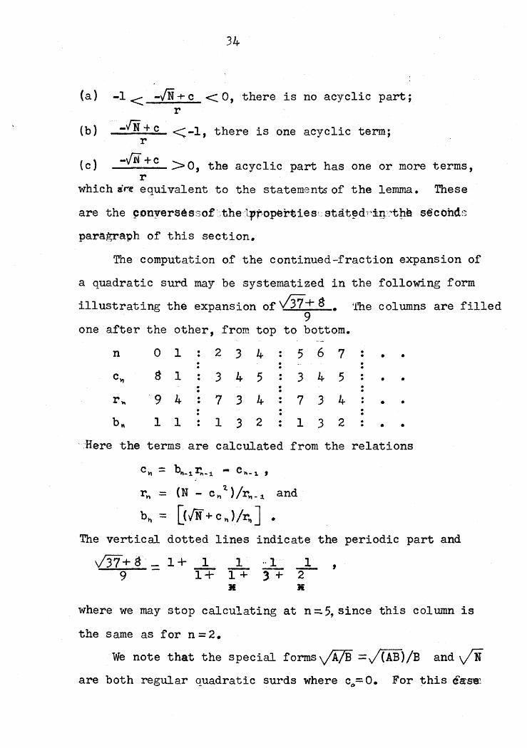
a quadratic surd may be systematized in the following form

illustrating the expansion of V37+ 8. 'The columns are filled9

one after the other, from top to bottom.

n 0 1 · 2 3 4 · 5 6 7 •• · · • •· ·· •Cl1 8 1 3 4 5 · 3 4 5· • •· · ·· · ·r", 9 4 · 7 3 4 7 3 4· • •· · •· · ·b" 1 1 • 1 :3 2 1 3 2· • •

Here the terms are calculated from the relations

rl'l = (N - C n 1 >!r".1 and

b n = [CIN+ c, l/r.. ] •

The vertical dotted lines indicate the periodic part and

v'37+ 8 ­9

1+ 1 1 ,·1 11+ 1 + 3 + 2

II Ji

,

where we may stop calculating at n =5, since this column is

the same as for n = 2.

We note that the special formsylAlB =J(AB)!B and Vi"are both regular quadratic surds where co=O. For this eaSel

35

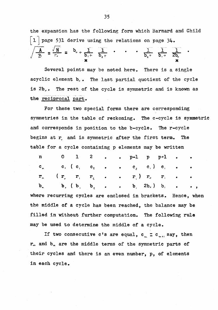
the expansion has the following form which Barnard and

[1] page 531 derive using the relations on page 34.

I; = :jr~ = Do + D~+ ~~: • • • b~~ D~+ 2~oH *

Child

•

Several points may be noted here. There is a single

acyclic element b~. The last partial quotient of the cycle

is 2b o • The rest of the cycle is symmetric and is known as-,,"'''~~'-

the reciprocal part.

For these two special forms there are corresponding

symmetries in the table of reckoning. The c-cycle is symmetric

and corresponds in position to the b-oyc1e. The r-cycle

begins at ro

and is symmetric after the first term. The

table for a cycle containing p elements may be written

n 0 1 2 • • p-l p p+1 • •

0.,.. Co ( c\ c t • • Cz 0, ) 0, • •

r"7'- ( r r, r-z. • • r ) r o r, • •OJ I

b.,.. Do ( b b • • hi 2b o ) b , • • ,z

where recurring cycles are enclosed in brackets. Hence, when

the middle of a cycle has been reached, the balance may be

filled in without further computation. The following rule

may be used to determine the middle of a cycle.

If two consecutive e's are equal, e~ : C~~I say, then

r~ and b~ are the middle terms of the symmetric parts of

their cycles and there is an even number, p, of elements

in each cycle.

36

If two consecutive r~ are equal and the corresponding

b ,,' are also equal, say r'llt = r""'fl and b?k =b?\(-t 1 ' these are the

middle terms of the symmetric parts of their cycles and c~r'

is the-middle' term of its cycle. Here p must be odd.

The expansion of jA/B and JNr are used extensively to

calculate solutions to Diophantine equations. Additional

relations, such as finding numerators A7\' , given the

denominators B~ and corresponding CIS and r's, have been

developed to simplify the calculation of approximants. In

other cases approximants are required only at one-cycle

intervals and relations have been developed to evaluate

these without the calculation of intermediate approximants.

7. Simple Continued Fractions for Solving Diophantine

Equations

(i) The equation ax - by =!l.

Kno~dng that a is prime to b, we wish integral solutions

in x and y. The determinant formula (IT-7) is used with

the following procedure. For ax - by : 1 expand alb as a

simple continued fraction having an even number of terms

and for ax - by =-1, do likewise using an odd number of

terms. Let the penultimate approximant be at/b'; the

I "'-,ultimate approximant being ab. Now ab' - alb = (-1) ,

so minimal solutions are

x = 'Of, y =at.

37

The general solution is obtained by putting

ax - by ="!. 1 = ab t - a ~b

in the form

a(x - b t } - b(y - at).

Now, since a is prime to b, blx - e', al y a' and

to give

x - bt =Y - at =t

b a say, an integer,

x =b t +- bt, y - a' +- at

the general solution as t takes on integral values.

(it) Pell's eauation x~ - Ny~ =! 1.

The first systematic solution to this equation was

given by Lord Brouncker in 1657. Euler wrongly ascribed

the solution to Pell and the name Pell's eauation has

remained.

To solve the equation ~ is expanded as a simple

continued fraction

1b1. T

• 1b1'\+-

12b o

*

•

Substituting bo + fi for the complete quotient after b., yields

IN =bo-t- blJ··~ • • b.~~ 1 • f~: ffli~:: t:/·I " I bo + j1t

Equating rational and irrational parts yields

A..... -I = NB"" b o 1"1"

B""_J - 1'l" b o Bn ,-

which substituted in the determinant formula (11-7) yieldsJ. ). ... -,

A~ - NB~ = (-1) •

. ,t =1, 2, 3, ••,

The general solution is obtained using the relation

Barnard andconnecting approximants one period apart.

Child [ 1 ] gi~e thiS, ge,neral solution as~ l' 'Z. .... _I

ArY' - NBt.~ = (-1)

where n is the number of elements in the period.

The existance of solutions to the two forms of Pell's

eauation denends on vvhether this n is even or odd. Thus#' .L

x~ Ny~: 1 has the solution, when n is odd,

t = 1, 2, 3, •••

and the solution, when n is even,

x : AZt ,. ,Y = Bzz)\ , t =1, 2, 3, •••

But x2. NyZ = -1 has a solution only 1t'lhen n is even, viz.

t =1, 2, 3, •• ; n =2m

and no solution for n odd.

(iii) The e quat t.cn ax - by = t. k ,

The solutions to this equation are obtained by solving

ax - by =.:tl and multiplying the solutions by k ,

Continued fractions are still being used in many current

investigations in number theory, for instance Barnes' and

Swinnerton-Dyer's [2J investigation "Inhomogeneous ~unima

of Binary Quadratic Forms."

39

8. Liouville's Proof of the Existence of Transcendental

Numbers

One of the most celebrated applications of continued

fractions to number theory is that of Liouville [12J who, in

1851, demonstrated the existence of numbers which are not the

roots of algebraic equations having rational coefficients, that is

~t, transcendental numbers.

To show this we first prove Liouville's lemma on algebraic

numbers, then construct a number which contradicts the lemma,

i.e. is not an algebraic number.

Liouville's Lemma 1I-2.

Given x D the root of an irreducible algebraic equation

with rational coefficients and whose degree n is greater than

1, then there is a constant c between zero and one such that

for any integers P, q we have

> s;qn • (II-26)

Proof.

when

The result is, of course, true for all n and all p, q

- x. j > 1, so we need lIm.~st'llgate'-(!n:ty for the casePq

X o ':::;1.I~ -Let X o be a zero of our irreducible algebraic equation

rex) = cox"+ C1 Xft

-1+ c,.x"-1. •••••

Now :r (~):f. 0, since :r (x) is irreducible, and

40

)

\

!'t, "-1

r r~q· = Cq p + C3:P q +. •\ q~

•

Also f(p/q) = f(F/q) - f(x O } = (~ - xo)f'(x j ) for some X:s.

between p/q and xo, by the Mean Value theorem. Thus

J(~ - X o) if (Xl) ~}. (II-27)

Now JXl - Xol ~ I~ .. X o 1~ 1 by assumption, so

JxI / ~ jxol + 1~ andit(xl)~Jn;Oxl~-L I + !(n-llC.l.x 1 .. •

LJ + ••• + IC~.L I

~ rfolCjx"i +1)"-1 + (n-l)lc].1 (IXoI+l)"·~ ••+ le"'11<lie,

for c bet~en zero and one and independent of p or q.

We substitute this result for fl(X1 ) into (II~27) to get

I"'·" 11~ - x, C >.Lq'"

,our deSired result, q.e.d.

~ve skatl now construct a number which does not satisfy

the lemma and hence is not algebraic. Let the number Xo be

expanded as a simple continued fraction

,• •Xo - b()+ 1 1 •- --b~+ b L +

whose elements are chosen to satisfy the relation that for

every n we can find a k so that

> )JbK+~ a, , (11-28)

..~is1 may be done in infinitely many ways, such as bK + :1. =1 + HI(.

Such a construction ensures that Xo is a transcendental number.

1B '" B z

I( I<

41

To prove this we shall show that if we choose any c,

O<:c~l, as small as desired and any n as large as desired

we can still find some p, q such that (II-26) of

Liouville's lemma does not hold.

(II-28) must hold for infinitely many k for any fixed n.

NOW suppose x D satisfies an irreducible algebraic equation of

degree n and having rational coefficients, then Liouville's

lemma holds. If we use (II-21) for the error in using Art/By!

to approximate x& and also our assumption (II-28), then

;~: - %0 < BKiKH < bk.~BK~ ~ B~ ltU •

for infinitely many k.

But no matter how small we choose c to begin with, weI··

can find an integer r such that ---r <c for all k ~ p. ThisBK

contradicts the result of our lemma, so Xo could not have

been algebraic.

Numbers found by the above construction are known as

Liouville numbers. 1bey have the property that if X o is a

Liouville number thenaXD+ b J.·S also a Liouville number,ex, -I- d

for a, b, c, d arbitrary integers such that ad - bc~O.

Hence Liouville numbers are everywhere-dense among the real

numbers.

42

III THE ANALYTIC THEORY OF CONTINUED FRACTIONS

Euclid's algorithm gives a method whereby a real rational

number may be expanded into a simple terminating continued

fraction. The extension of the method to a rational

polynomial function follows at once. The expansion of

irrational numbers as non-terminating continued fractions

suggests that an afla~ogous treatment of infinite series

representing real-valued functions may be valid. this is

true within limits.

A quadratic equation having real roots may be manipulated

to yield a continued-fraction expansion converging to the

larger root. The same manipulation applied to a quadratic

equation having complex roots yields a continued fraction

which does not converge, but 1JhtchsmajtJ",~~H~:itlla-ee'.:.n'l1iU;c~

x - x - 1 =0 may be written as

x.1+1x

1+ 1 1 1= n- 1+ 1+ • • • • • f

which converges to the larger root (the golden ratio).

However- x 2. - X + 1 :: 0 may similarly be written

x • 11--x =1 1 1 1- 1- 1- 1=

• • • . . ,

which takes the values 1/1, 0/1, -1/0 cyclica11j:y,whereas'~bhe

roots of the equation are complex.

When expanding functions as continued fractions we are

concerned vnth the similar possibility that the expansion

may not converge. This is the convergence problem, the central

theme of the analytic theory of continued fractions.

43

Another desirable extension is ~en~rallz1ng~wtth the

elements of our continued fractions beihg complex numbers.

The most satisfactory approach to the convergence

problem is that developed by Wall and his associates [17J.Their method is to regard the continued fraction as being

generated by a product of linear fractional transformations

in the complex plane.

1. Continued Fractions as Products of Linear Transformations

Given a linear fractional transformation of the form

•. ~

.~ +~ -Dn/.i n ,. .J.,,_~ J)'\ k; + w

jy\

where the transformations are applied in the order

44

'.,'Renami.ng our parameters thus

and defint,ng

,

a h +1 =- Dh• 1-J)t

to = b cs + w, t p = a e

b" +w

we get our familiar form of continued fraction to be the

product of the transformations

t. t 1,. - . - -E.... +w

• (III-I)

For an infinite continued fraction we note that"'('hhe~'

.yalue:/of 'the:f.:eaction is

lim to t 1 - - • t t\(O} =n-)oo

lim tot1- • • t..,( ex» •n~oo

(111-2)

The nth approximant is given by

tot:L • • • t n (~ ) =tot1. - • t l"tt Y) t 1.(00) = Al'\ /B n • (111-3)

The recursion relations and determinant formulae of

section 2 of chapter II apply, since we derived these with

no restrictions on the elements.

We now establish an important connection between

continued fractions and infinite series as our first tool

ft>,. investig~tl1l convergence. \Ve neglect the leading bo and

first partial quotient a 1 / bI , as these do not contribute

to convergence.

Theorem III-I.;

If the denominators Bp~ 0 for

- • • • , (III-4)

45

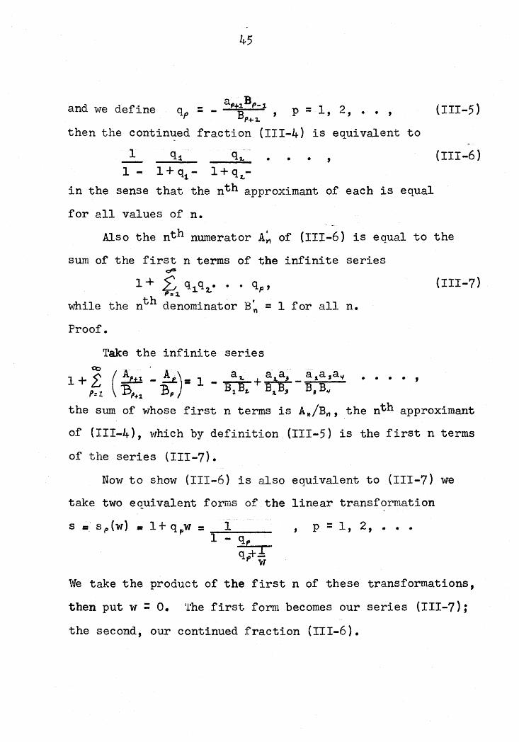
and we define

I

qp : a"tB1Bp-1,~ p =1, 2, •• ,P+l.

then the continued fraction (11I-4) is equivalent to

(111-5)

(1II-6),•••1 q1 q~

1 - 1 + q1 - 1 + q l.­

in the sense that the nth approximant of each is equal

for all values of n.

Also the nth numerator A~ of (111-6) is equal to the

sum of the first n terms of the infinite series~

1+ £ q1.q %,. • • qp'/1:::1,

~mile the nth denominator B~ = 1 for all n.

Proof.

(111-7)

Take the infinite seriesQ::) ... ..... .... .. •

1 + Pl,l (it' -~')=1 - B~B~ + s:;; -::::a. ....,= P+1 (J

the sum of whose first n terms is AM/Bn , the nth approximant

of (III-4), \4fhich by definition (111-5) is the first n terms

of the series (111-7).

Now to show (111-6) is also equivalent to (111-7) we

take two equivalent forms of the linear transformation

, p =1, 2, •••

We take the product of the first n of these transformations,

then put w =o. ~he first form becomes our series (111-7);

the second, our continued fraction (III-6).

46

To show the nth denominator of (III-6) is 1, we note it

is true for n =1 and n =2, and our recurrence formula

gives, (assuming Bn =1, n =1, 2, . . • ,k),

2. The Even and Odd Parts of a Continued Fraction

We are interested in the form of the even and the odd

parts of a continued fraction in terms of the elements of

the original continued fraction, since we may sometimes prove

convergence by showing that the even and odd parts separately

converge to the same limit.

. . . ,For- simplicity we take the form

1 a 2.. ....!.J1+ 1 + 1 +

which has the even part

{III-B}

11+a2.-

aLa?

1 + a, + at -• • {III-9}

and the odd part

1 - a 3,.

1+a L + a 3 - l+aCf+a~ -• • • • (111-10)

We may transform (III-B) into other forms as mentioned

in section 1 of Chapter TI. Hence, to fina the even or odd

part of another form we transform (III-B) to the desired form

and apply the same transformation to the elements of (III-9)

or (111-10). Any leading term b o must of course be added.

47

To derive the even or odd part of (III-B) we regard {tII-B)

as being the product of the transformations

. ,p = 2, 3, •=w, 1l+a pw

so that (for example) the odd part must be generated by

the transformations

r 1 (w') =t ~ (w) =w,

which gives the odd part in the form (III-lO).

The even part is similarly derived. More general

"contraction" (and also "expansd.on") formulae may be

deduced when required.

Convergence Conditions

By convergence conditions we mean the conditions on the

elements ai, bl which ~dll ensure that the continued fraction

will converge. It seems intuitively clear that if a partial

numerator is zero, then the preceding partial denominator is

not being changed and the fraction is in effect terminated at

that point. However, it is not this simple, since it might

happen that we still have infinitely triainti B,,:'O and hence divergence

by our definition. Hence the following theorem is important.

48

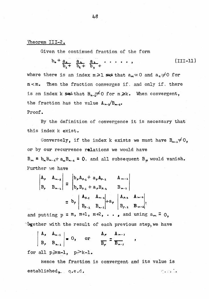
ff'heorem III...2.

Given the continued fraction of the form

bo +.!.L... !:.J..... .!h- • • • • • , (III-II)b 1 + b, + b, +

where there is an index m~l SiOft that am - 0 and a.,:fO for

n < m, Then the fraction converges if. and only if. there

is an index k $ltG.h thatB.,_~ ° for n ~k. When convergent,

the fraction has the value A~-JB....s.

Proof.

By the definition of convergence it is necessary that

this index k exist.

Conversely, if the index k exists we must have Bm_~-i0,

or by our recurrence relations we would have

Bm =bhtB""'-1+ ~B",,_1. =01 and all subsequent B)O wouLd vanish.

Fur-ther- 1'le have

BI'-- bpB'.l +a pB ,o_2. B"",-1.

!.p.., A"-1 Ar-~ A",.sj= b, +a, ~B,-.1 B'ft._1 Br_:t BWI- ....

and putting p =m, m+l, m+2, •• , and using am =0,

·'·t"ether with the result of each previous step, we have

A, AW.-l A.'f' A",,-.1• 0, or -

B" - ~J,

for all p;:::m-l, p?k-l.

Hence the fraction is convergent and its value is

establishedt- q. e •d •

49

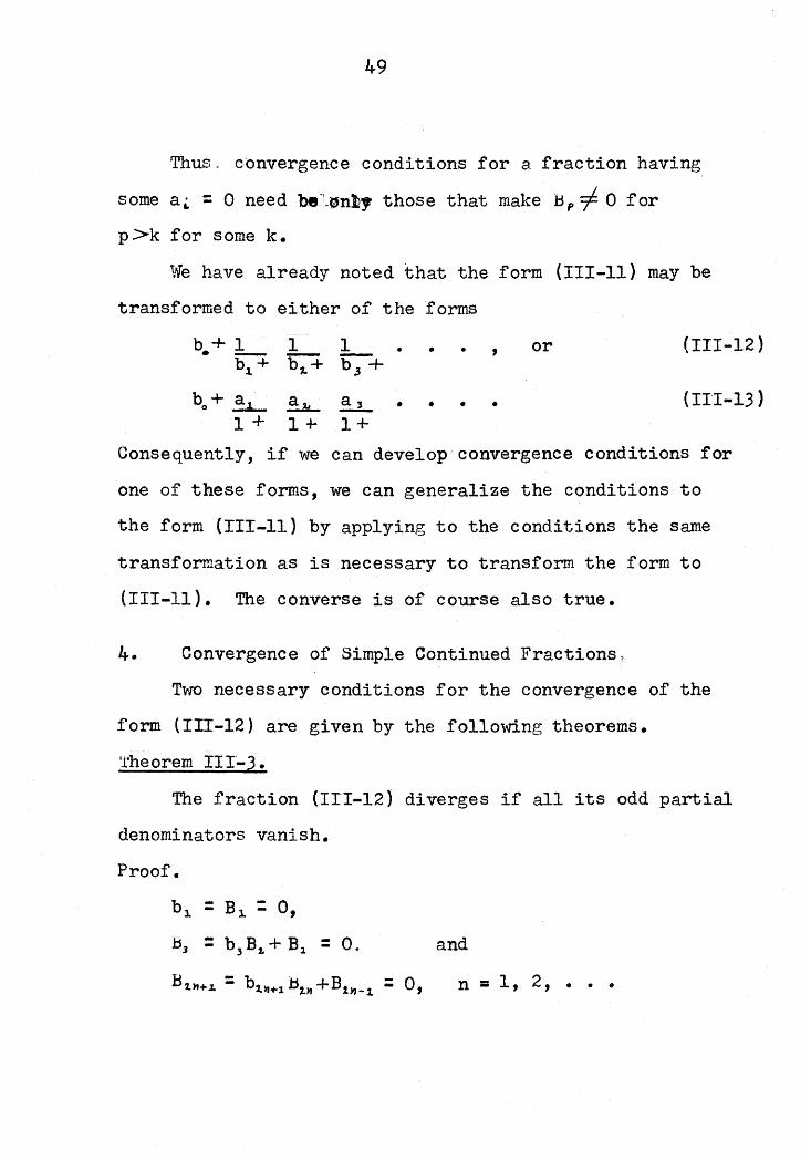
Thus convergence conditions for a. fraction having

some a L = 0 need be"l.,n12, those that make Bp =I- 0 for

p>k for some k ,

We have already noted that the form (III-II) may be

transformed to either of the forms

b. + 1 1 1 • • or (111-12)bJ. + b~+ b.3 +

,

b+ !..l..- !.J£... ~ • • • • (111-13)0

1 + 1+ 1+

Consequently, if we can develop convergence conditions for

one of these forms, we cangenera1ize the conditions to

the form (III-l1) by applying to the conditions the same

transformation as is necessary to transform the form to

(III-II). The converse is of course also true.

4. Convergence of Simple Continued Fractions

~ro necessary conditions for the convergence of the

form (III-12) are given by the following theorems.

'l'heorem III-3.

The fraction (1I1-12) diverges if all its odd partial

denominators vanish.

Proof.

bl. =B~ =0,

Jj3 =b, B20 + B1 = O. and

n =1, 2, •••

50

Theorem 1II"4. (A Theorem of Von Koch).

If the series 2:/bp l converges, the form (II1-12)

diverges. The sequences of its even and odd numerators and

denominators, {Au}, r~PT1}' {B~p 1, {B1PH]converge to finite limits Foo ' F1 , Go' G1 respectively and

F~ Fo

=1.G1 Go

Proof.

Since bo does not contribute to convergence we shall

use the form

• • • • • (TIl-II..)

etc., to

= b;LP A..,. % + b~p..lA1.P-.3 +. • • + b, AI

= £ b.tr A1 "_1.NO~l if we show"bhHt I A'Lp-J. ,<. C, a constant independent ot p,

then f Al~1 converges ,

Let M be the greater of IA_1 1 and I Aol, where A_ l =1.

Then I11 I~ Ib1 I· lAG 1+ \A_ 1 I~M(l + l bI ,),

IAt I.:::; 1b>. I- tAl l+ IA. I::::; Ib,,\M(l+ hI. b+M

~ M(1 + Ib:1 1) (I+ I b 1. I) ?

and by induction

lAt\ I~ M(l+f btl )(1+1 b~ I.)n =

• • • •

1, 2, •

(1 +r b~ I>;• • •

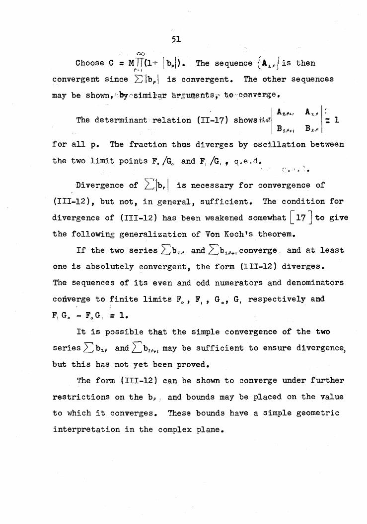
5100

Choose C = MTTCl+ Ibpi). The sequence {A i P1is thenP:./

convergent since L;·lbp I is convergent. The other sequences

may be shown,I-.Oycsinrirgr a?gtrmerreSr 1iQ~'c,~nve:r,ge.

The determinant relation (II-17) shows n.a : 1

for all p. The fraction thus diverges by oscillation between

the two limit points Fa IGo and F, 10, , q.e~d.

Divergence of L"lbp I is necessary for convergence of

(III-12), but not, in general, sufficient. The condition for

divergence of (III-12) has been weakened somewhat [ 17 ] to give

the following generalization of Von Koch'S theorem.

If the two series 6b1.p and ,L01P+I converge and at least

one is absolutely convergent, the form (1II-12) diverges.

The sequences of its even and odd numerators and denominators

converge to finite limits Fo ' F, , Go' 0, respectively and

F, Go - FoG. =1.

It is possible that the simple convergence of the two

series .L: b'2..p and L b2 P+1 may be sufficient to ensure divergence,

but this has not yet been proved.

The form (ITI-12) can be shown to converge under further

restrictions on the b p and bounds may be placed on the value

to which it converges. These bounds have a simple geometric

interpretation in the complex plane.

52

Theorem 1II-5\~

Given the form (III-l~) whose partial denominators bp

satisfy the conditions

6(b, ) >0, rR (b" ) ?O, p =2, 3, • • ., (III-15 )

thal twe series L:: IbLp~, I and L IbLP+'spLI both converge, where

sp : b, + b~ + • •• +92.p, and finally limit s p = CD. Then

the fraction converges and its value, v, satisfies

•2 (R(b I )

V -----1 ~

Proof.

Consider (III-14) to be generated by the transformation

The conditions(III-15)'I'············· ...··tr·.~'w·

1; = 1; p (w) ,. b ..• -, .., P .r. •p + W b

p+- W 1-

showc that each transformation maps the right half-plane

O{,.(w)?O into the right half-plane a( (t)~ and'that tne-ffirst

transformation maps (f( (w)~O into the circular region

t - 2 itCh,) ~ 2 (R.(b, )• (ttt -16)

... ...~

Hence the transformation t =tit 2. • • t pew) maps a:2.(w)~llti>nto

the same circular region~ and,since t,t k ••• tp(O) =Ap/Bp,

the pth approximant \ l~ ~~ .Now the restriction on b, ensures tbat b, -=/:- 0, bence

every convergent is finite. Also limit sp = (I) ensures that(I)

the limit Ap/B" converges and hence this limit must be

finite.

(1) A number of long theorems le~d~ up to this resultare omitted for brevity. See Wall L17J , pp.28-32.

(111-17)

53

Since every approximant is mapped ,into the circular region

(III-16),it follovm that the value of the continued fraction

must also be found there.

5. Continued Fractions Having Unit Partial Denominators

In studying the form (111-13) we noted that bo and a 1

did not contribute to convergence, so the modified form

(III-B) is equally suited to our study of convergence of this

type of continued fraction. We shall define relations termed

the "fundamental inequalities" for the form (III-8) and give

these inequalities certain interpretations for particular

cases.

\f{e say th(tt form (III-B) satisfies the fundamental

inequalities if there exist numbers rh~OI such that

r p 11 + a, + a'+1 I?::: r p rp- L Ia.. J+ J a p+1 l, P = 1, 2, • • •

vie also define a 1 = r_1. :: r o = 0, to give

Ii Il+a2.l;::: la2.l, for p =1, and

r. 11+ a1. + a.l.;=;: Ia.3l, for p = 2.

The follo\dng theorem gives the first interpretation

and application of the f~~damental inequalities.

Theorem ITI-6.

If the continued fraction in the form {III-8} satisfies

the fundamental inequalities (III-17),then the denominators

Bp =1= 0 and the

Iq e1~ r p ,

qf =-apf J.Bp- l 1 satisfy the inequalitiesB'.,.l

p =1, 2, •••

54

Proof.

By our fundamental inequalities for p =~, p =2, we see that

Bt. = 1 + a2 =F 0, B3 =l+a:L+a3 =1= 0,

[qll = aZ, ~ r 1 , [q I - 1 a.3 ~ r.z.1+a1 1. - l+a2,+aJ

and then use induction for the two possible cases of

a k+~ = 0, and ak'-r1. =t- 0.

For aK+1- • 0,

Bk+ to = BI<+1+ al(+1 BI<= BK +~ =1= Of and

Iqk+ll = aN+1B~ =°~ r"+1 •BIC-f. 1.

Now when akt2.=FO, the fundamental inequalities show that

when p =k+l, it follows that rJ<+1:::>O. Our recurrence relation

(II-G) shows BIC+ 2. = (1 + af<+1 + a k+ 1. )Bk - al< al<+lBk-:L. This we

combine with our induction hypothesis and the fundamental

inequalities to get

! BI<+l =11+ ak''t 1.+a 'c+z.

a/(;~Bj( a k.,.J,

~ 1+al(+1+ al<+L

ak+l.

~ -..L >0.rl(+1

Hence Bkt1=f 0 and IqkUI~ r kU •

Corollary III-I.

If the continued fraction (III-8) satisfies the fundamental

inequalities; and some a p • O,the fraction converges.

55

When the continued fraction (III-B) satisfies the

fundamental inequalities (III-17), thetS"E~e~

1 + L r I r 1.-. • • r" is amajorant for the series 1 + Z CI,. • .qp'

which,by theorem,III-l,is equivalent to the fraction. This~""---'-'-"'-'-'~ -•. <.' •

is called the first interpretation of the fundamental

inequalitie.. This may be demonstrated by proving

Worpitzky's theorem, where suitable restrictions on the a~

permi t corresponding r p WAfcb e'ns.~ure v,;t.6nller~l}e;ne~ t:o".J3·e tt:~W1d •

(Worpitzky's Theorem).Theorem 111-7.

• • . , be functions of any variable'- over

a domain D in which

Ia,l < 1/4, p =2, 3, •••• (11I-18)

Then (a) the fraction (III-B) converies uniformly over D,

(0) the value of the continued fraction and of its

approximants lie in the circular domain

Iz - 41:31 ~ 2/3, (III...19)

(e) the constant 1/1+ is the ''best' constant that can be

used in (III-18), and (II1-19) is the tbest' domain of

values of the approximants.

Proof.

(a) Using the restriction (III-18),

r1 + a ,-13 j (1 ~ ~) = i 3 Ia ,-I

11+ a,:l-a,l ;:0 ~ ( 1 ~ ~ - ~) ~ !

we write

,3 \aJ ,

56

l~.211+ap+ap+1I;?:2(P~2f =p!2°P. ;2o~ +~

;?: p~2 P -/ Ia p ]+Iap+:L!, P = 3, 4, • • •

This satisfies the fundamental inequalities with

Now• •p =1, 2, 3, ••

co

o or, = 1+ ,f ~.~}~ · 0 0 • p~"2

=1+ cSo 2L (p+l)(p+2''=1.

=1+2 ~(-L _1) =2.i..J p+l P4- 2"~1

Our majorant series converges uniformly, so the fraction

rp =. 1> _'P+"2 'eo

1+ L r.t rio •f-:2

converges uniformly. r£he modulus of its value and the moduli

of the values of the approximants do not exceed two.

(b) We write w =rt i~ i'+ · 0 • , IxJ~ 1,

to put the continued fraction in the form

so solving (111-20) for w we have

or Iz - 4/3 f; 2/3.

z = 1 ,l+tw

By (a) we kkp.iu)ttu. t Iw I~ 2,

Iw 1= 41~1~2,

(I1I-20)

Since any approximant may be written in the form (I11-20),

<~,.t::· must s l.so lie in (111-19).

(c) To see that 1/4 is the 'best' constant,we put all aL =a.

in the denominator of (III-B) to get

• • • = 1 +!: ,x

that is x1. _ X - a =0 •

57

This continued fraction will converge to t~troot

.L.

1!'(1+ 48.)2. of the corresponding equation whi"c.h "has'~the2

larger modulus, except when a is real and a <-1/4.fZ)

In the latter case the value oscillates.

To see that (111-19) is the 'best' domain,we take

• , in our fraction,soai • - 1/4, i = 3, 4, 5,

z =1 .!J... 1L!L 1L!L.1+ 1- 1 - 1-

• •

• • - 1 •-, i + 2a2.

As a2. ranges over the domain (III-IS), z fills (II1-19) r,

, ..-.The theorem may be extended by replacing (IIT-18)

by r a, I~ r(l-r), o<~1/2, lrhen the domain of values

becomes 1 1& "rinstead of (111-19).z - 1 - r· ,2. -;.;::: 1 _ r 1"

The second interpretation of the fundamental

inequalities follows from the following theorem~stated

without proof.

Theorem III-B.

Given the continued fraction (III-B) which satisfies

• •p :: 3, 4, •

the fundamental inequalities in the form

r 1 11+ a 2.1~ (1 + k, ) Ia 2.. 'I, kI ~ 0,

r~ rl + a'L + a.31 ~ (1 + k%,) fa., I, k~ ~ 0,

rf II+ ap -l- a,+~ I~ r, r,_z lap 1+Ial'f-.1 ,~

'rhen if k1>O, (kz.>O), the even (odd) part of the continued

fractioncoI1verges.

(2) This point is based on a theorem, not quoted, SeeWall [17J , Theorem 8.2, p. 39.

58

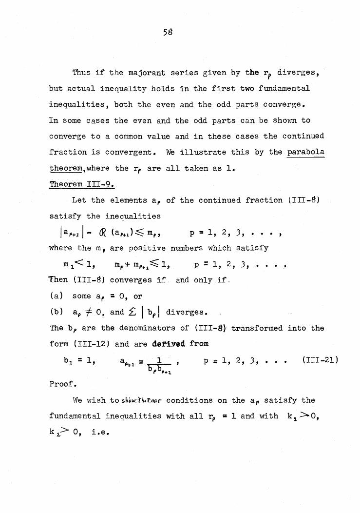
Thus if the majorant series given by the r p diverges,

but actual inequality holds in the first two fundamental

inequalities, both the even and the odd parts converge.

In some cases the even and the odd parts can be shown to

converge to a common value and in these cases the continued

Proof.

p =1, 2, 3, ••• (111-21)

We wish to >hb~ctkcf'~j)r conditions on the ap satisfy the

fundamental inequalities with all rp =1 and with k 1 ~O,

k ~> 0, i.e.

59

Il+a.I>/a.t,Il+a2-+a 31:>- la 3 / ,

1 1 + ap+ap"'ll~ lapl + /a,+l!. P =3, 4, • .'.Well

!1+a11 ~l+ !R(aL) :;?l+ laL/- m,> raLI,and /1+ afl+ap+II~·l+ CR(a p) + <R(ap+,)

~ 1 - mp_ , - m,,+ [apj+ /ap+,/~Iapl+lap+lj, p =2,3,4, ••• ,

where it may be 11 + a;l+a 3 / = (a 3 1, if a:L = O.

If some a p : O,we have convergence by Corolla~ III-l.

If a,. -=1= 0; for p =2, :3, • • , the diver-gence of 2: Ib, Iis necessary for convergence. It can be shown (3) that when

the a p satisfy the fundamental inequalities, the:", t

divergence of L Ibpi is sufficient to ensure convergence of

the even and the odd parts of the continued fraction to the

same limit, q.e.d. . . '.,.A geometric interpretation of the theorem is that each

a p must lie within or upon the parabola haVing focus at the

origin and vertex-mp _ ,! 2 . Also if the pth parabola contains

real values less than -'k, then the p + 1th parabola cannot

contain -!, the limiting value of a p+ , in Worpitzkyts theorem.

The above theorem leads to the parabola theorem where

m" =1./2 :f'C)x-., all p, Each parabola then

(3) A number of long theorems le~d~g up to, the3e resultsare omitted for brevity. See Wall L17J , pp. 5~-;6.

60

contains Worpitzkyts circle I a p I:::::; 1/4, and we have an

extension of the value '-region of Vlorpitzky's theorem. t1his

extension of Worpitzky's theorem is stated without proof.

Theorem III-IO. (The parabola theorem).

A set, S,of points in the complex plane, which is

symmetric about the real ,axis, is a convergence set for the

continued fraction (111-8) if. and only if S is a bounded

set contained in the parabolic domain

I z I - rR. (z)~ 1/2. (111-22)

If the a p of the fraction (111-8) lie in this

parabolic domain,the fraction converges if, and only if

either

(a) some ap :: 0, for P = 2, 3, • • • , or

(b) a f =/ 0 and 2.- Ibp I of (III-21) diverges.

The values of the fraction (IIT-8) and of its

approximants fill the domain

z -=1-0,as the ap range independently over the parabolic domain

(111-22) and satisfy (a) or (b).

6. Extensions of Convergence

A sufficient condition for the convergence of (III-II)

is that I a pI+ 1~ Ih" 1, analogous to the definition of a

proper continued fraction. Worpitzky's condition becomes

for this form. A ratio test analogous to that

61

for infinite series.. is .th.·at a-ii'~7b~_i I <1, from and after

some index n, If I:~~'::~' I>l,a~h:~fraction diverges by1'\ ...... ,

oscillation. In the case of equality no conclusion may be

drawn.

Certain classes of continued fractions having special

forms have been studied and corresponding conditions for

convergence have been deduced. For example, the continued

fraction of Stieltjes, or S-fraction, has the form

1k,s +

1 1kLf+

. . . . ,

where the partial numerators are ones, the k's are real, and

positive and the z appearing in alternate partial denominators

is a complex variable.

Another type of continued fraction has the form

1•.•.. ~- 2-

at a:zb2,.+ 3'2,. .. b 3 + 3 3 - bt+ + 3.,. -

. . . , (111-23 )

where the a's and its are complex constants and the z's are

independent complex variables. If all the z's are equal to

a common variable z, this form is known as a J-fraction,from

the related quadratic L {Df + ! )x; - 2L a, xrx r... " called a

J-form.

By specializing form (ITT-23), an extension of the

parabola theorem is obtained. Tn this case, when the fraction

is transformed to the form (III-g), each partial numerator

must lie 'Within a parabolic domain, focus at the origin,

but axis not necessarily on the real axis.

62

This domain for each a~ of form (III-B) is determined by

the elements of the form (111-23). The domains for the

a L do not necessarily coiDcide.

Another problem in the analytic theory of continued

fractions is to establish 'value regions' corresponding to

certain convergence sets. For example,the convergence set

I apl~1/4;of ~vorpitzkyts theorem gives rise to the value.

reg:i.ort Iz - 4/3\::::;: 2/3, in which the value of the fraction

and the values of all its convergents are found. 11he

parabola theorem similarly defines a value region

!,z - 11::::;:1, for elements contined in its parabolic

convergence set. This problem has been solved for many

special forms of continued fractions but general solutions

are as yet lacking.

63

IV REQUlRE~~NTS FOR CO~~UTER APPLICATION

We shall now investigate the suitability of continued

fractions as a means of generating approximations to function

values in an electronic computer. For this application the

basic points to remember are (a) functions may be expressed

as convergent continued fractions and (b) the continued

fractions may be transformed into different forms.

The choice of a method for handling a particular problem

on a given computer will be governed to a large degree by

the operating characteristics of that computer. Howeve~ the

general principles of computer operation do allow us to

formulate a few reauirements for using continued fractions

for computer approximations. For the sake of completeness

we shall review briefly the general operations of

electronic computers.

1. The Turing ~~chine

A. M. Turing in England appears to have been the first

to classify the essential operations involved in numerical

computation regardless of the mechanism used--mental, pencil

and pa.per, desk calculator, or more sophisticated business

machines. The computational process involves the follo~rlng -

arithmetic operations,

6torage of data and intermediate results,

64

shifting data from one storage to another,

input of raw data and output of final results,

making decisions based on intermediate results and

miscellaneous control operations.

As a result, stored-program digital computers are often

referred to as 'Turing machines~ although Charles Babbage

designed a machine such as this over a century ago.

The operations enumerated are performed without conscious

thought when calculating with pencil and paper or with the

aid of a desk calculator. The emphasis is on the arithmetic

function although a general plan is followed in solving

the problem. Decisions about detailed procedure and about

changes of procedure are made as computation proceeds. Non­

productive time used to copy or shift intermediate results

and for making decisions results in the inefficient use of

even a moderately~fast desk calculator. Eleotronic computers

are many orders of magnitude faster than desk calculators,

so the whole sequence of operations required to solve a

problem must be pre-planned So that the computer may work

ef£:tciently. In addition to arithmetic operations and

shifting and control of data, tests must be provided at each

point where the result of previous computation mj~ht determine

the course of following computation and alternate sequences

of operations tpttst"oept'Cltided for each such test (decision).

65

This pre-planned sequence of operations which the machine

is to follow is known as the program.

Electronic digital computers are provided with the

following basic functional units of the Turing machine.

Input-output devices introduce instructions and data

into the machine and extract the ~su1ts of computation.

The arit<h.1'Ii'etic unit must perform at least the basic

operations of addition and subtraction. Multiplication and

division can be accomplished by repeated addition and sub­

traction under program control but more commonly these are

basic operations of the arithmetic unit. Special-purpose

machines may be provided with other operations such as that

of taking the square root. Any arithmetic operation not

performed by the arithmetic unit as a direct operation must

be accomplished under program control using those operations

which are available.

A.ee~umUiat0'rS orre'gister's in which numbers are placed

to be operated upon and in which results of arithmetic oper­

ations appear. There is usually at least one accumulator

and sometimes several. At least one of these should be capable

of performing all the allowable arithmetic operations while

arithmetic in the others may be restricted or non-existant.

66

The data capacity of the accumulator varies, but is usually

modest, the average being of the order of 8 to 16 decimal

digits. The 256-eharacter capacity of the IBM 705

accumulator is exceptional.

Mertlory orinrorntation's'toraiEEi is usually taken to refer to

storage where information is placed until required for

processing, but where no arithmetic operations are performed.

Accumulators are then conSidered as adjuncts to the arithmetic

unit. This distinction is not clear for machines which

perform limited arithmetic operations without recourse to

the accumulators. The data-storing capacity of the memory

is finite, though very large, in some machines. lvlemory must

be systematically subdivided so that stored information

may be referred to by its location, (known as the address ),for storage and retrieval. These memory subdivisions are

variuusly known as words, numbers,ceiis, sectors or other

designations. and correspond to the basic units of information

handled by machine operations. Some machines also handle

multiples of this basic unit simultaneously in some operations.

Word length varies from a single alphanumeric character or

digit to the equivalent of ten or more decimal digits. For

technical reasons information is usually handled within the

machine in binary representation. This may be a simple

67

binarization of purely numerical information, or may be a

binary coding of individual alphanumeric or decimal characters

handled by the input-output devices.

The control function is handled by many different

components located thro~~hout the computer. They combine

to interpret instructions in the program sequentially and

properly synchronize their execution.

These functional relations are conveniently shown in

the diagram of fig. IV- 1

Control

Arithmetic

Functional Relations of a Computer

Fig. IV-I

The instructions making up the program are so much more

data the machine must handle so are represented in the same

form as other data. Program and data are distinguished by

being located in different addresses of the Same memory.

68

The machine then treats a given piece of information in

memory as a program instruction or as a piece of data solely

upon the basis of previous instructions (manual or

programmed) and not upon the form of the irdbrt,arl"fl. This use

of a common memory for program and data has both advantages

and disadvantages. A single memory is more economical of

storage hardware requirements than a double memory but it

makes the destruction of a program much easier due to

incorrect coding or machine malfunction. trhe most-,

important advantage is the ease with which changes may be

made in the program. A given sequence of instructions may

be used repeatedly, each time on different data, or using

different constants on the same data. After the arithmetic

operations of the sequence are completed,further instructions

in the sequence make the necessary modifications to the

sequence itself. Finally a test must be made to detemmine

when to terminate the iteration of the process.

This repetition of a sequence of operations in a

computer is known as looping and the sequence as a loop.

It may be simply regarded a~-a mechanized algorithm. The

decision to end the loop may come after the loop has

operated a fixed .umber of times, or may be made when the

contribution of one iteration of the loop ceases to have

significance for the computation in hand. An example of

69

the former is the evaluation of a function at a fixed nwnber

of values of the argument. The latter might be used in a

square root process which stops after reaching a given stage

of accuracy. Different tests would apply in each of the two

cases.

Subroutines

Some problems recur frequently as parts of the solution

of larger problems, as for instance square roots, circular

functions and exponentials. It is inefficient to write the

reauired seauence of instructions in the main program each~ ~ ~

time it is required. fThese problems are therefore usually

written as short and optimally efficient or optimized

programs known as subroutines. Irhe main program then refers

the evaluation of the function to the subroutine which in

turn returns control to the main program after performing

its function. In this way one subroutine may be referred to

from many places in one main program, or many programs may

refer to the same subroutine. In effect, subroutines provide

the computer with operations which are not built into the

arithmetic unit. 'rheae operations are called into use by

pseudo-instructions or calling seauences. Subroutines may

be used to evaluate functions, perform special computations

(such as computations with complex numbers), control and

check input-output functions "an.~:'_do··m~n:V·_,Qthe.:r: things.

70

A subroutine for e valuating functions should be both

rapid and accurate. Speed depends on the rate of convergence

of the method and the manner of using the method. Accuracy

is impaired by round-off errors and by truncation errors.

We have mentioned that a computer will handle numbers of a

rather limited size. Hence all numbers except a comparatively

few rational numbers which are smaller than the limiting size

must be handled as approximations. For practical purposes

we may say that a given machine handles numbers with a

round-off error characteristic of that machine, that is~I/2

a unit in the least significant position. This small round­

off error is usually negligible even if compounded through

a few arithmetic operations. For a large number of operations

most of .ntctrj"1 may be expe cted to cancel each other out.

Hovrever, being random errors,they should accumulate

according to the theory of random walks, that is, the

binomial distribution. We then try to keep the number of

arithmetic operations to a minimum to reduce the possibility

of accumulating large round-off errors and also to speed

the operation of the subroutine.

The truncation error caused by terminating the process

after a finite number of steps may be more serious. wnile

theory may jjl~i(~itt,·ttiA~~ certain number of terms will provide the

desired accuracy and that the last few terms used '

71

contribute to this accuracy, the last few terms may, in

fact, be individually smaller than the characteristic

accuracy of the machine and so be lost. In such a case

we use the Same process but a different method of calculation,

or we look for another process to yield the desired accuracy.

To be suitable for a computer subroutine, any approx­

imation method should meet the following requirements.

(a) It should be an algorithm whose iteration consists

of relatively simple steps, and

(b) each step should involve as few arithmetic operations

as possible.

(c) It should have rapid convergence so that the desired

accuracy may be reached in a few iterations.

3. Series and Continued Fractions for Subroutines

Series expansions are commonly, used for, evaluating

functions in computer subroutines. We shall, examine their

suitability, as well as that of continued fractions.

Only a finite number of terms of a series can be

evaluated, that is, a truncated polynomial is used. The

point of truncation may be determined in one! of two ways.

Evaluate the series term-by-term, st.oppj.ng when the

last term does not alter the function value calculated.

72

That is, it has become smaller than the characteristic

accuracy of the machine. The advantage is that the loop

ends as soon as the desired accuracy is attained; only the

last term evaluated ,"'1:'5 ~ redundant. 'lile disadvantage lies

in the extra operations required to determine when the last

term has become insignificant. ~ince this test must be

repeated at each iteration,it takes longer to evaluate each

term. Now for slowly converging series,manYiterms may be

neglected (being smaller than the computer ro~d-off error)

while their cumulative effect is far from negligible. We

therefore try to work ~nth alternating series whose truncation

error is less than the last term neglected. iAlternan~l~we

may hasten convergence by using some contraction operation

which,in effect,allo~re us to evaluate several terms as one,

but often complicates the law of passing fro* one term to the

next. The better remedy is to use a different method.

Secondly we may determine beforehand the maximum number

of terms required to evaluate our function t~ the required

accuracy for any value of the argument within its range.

The number of terms of the series is then fixed but no testing

is necessary to decide when a term becomes insignificant.

To avoid the illusion of accuracy which may ~e lost by

evaluating insignificant terms, we may alter the method of

evaluation s~,Jth'al:'t)n~,ct~'tlr1will have its contribution neglected.

73

For example, we may write the six-term trunoated expansion

of eX in any of the forms

(IV-l)

Thus truncated series are suitable for use as subroutine

Continued fractions resemble infinite series in many

respects in the way they fulfill the requir$ments for

computer subroutines. Again the form is tr~ncated for

evaluation. The point of truncation may be!determined in

either of two ways. The first uses the rec~rsion formulae

(II-6) to evaluate successive approximants. Each

approximant is tested to determine when the change from the

previous approximant has become less than machine round-off.

The evaluation process stops when the desir~d accuracy has

been attained, the last evaluation being redundant. In each

loop extra operations are required to perform this testing.

We are again faced ~~th possible slow convergence and

consequently the possibility of neglecting terms which are

74

not insignificant. To avoid this difficult~ we may try to

obtain a proper continued~fractionform. Approximantsare

then alternately larger and smaller than th~ desired

approximation and the truncation error smalller than the

change introduced by the next approximant. A1te~ly we

may hasten convergence by.:'.a contraction method, as for

instance evaluating the odd or even parts o~ the fraction.

This will usually complicate the form of the fraction. As

with series, a better remedy is to find the' point of

truncation by another method.

The second method is to determine the number of partial

quotients required to give the desired accuracy for the

function for all values of the argument within the domain

used. No tests for convergence are then re~uired, but the

number of iterations is fixed for every value of the argument

which may be used. The computer then eval.uabes the continued

fraction starting with the last partial quotient.

Thus truncated continued fractions are' also suitable

for a subroutine algorithm providE~ that a' rapidly­

converging form can be found.

We note in passing that for infinite series and for

continued fractions the second method of evaluation permits

the elimination of the loop in the program.

75

Since the number of iterations is fixed and ifew, we may

elect to repeat the sequence of computer cOIl\lands for each

iteration for the required number of iterat~ons. This

saves the computer commands and operating time required

to count the number of iterations. This results in a faster

running program at the expense of few additional commands.

It is important to bear in mind that t»e operating

characteristics of the computer to be used nave a strong

bearing in choosing the most suitable algorithm for a

subroutine. They may also be a factor in d¢ciding the

method to be used in evaluating the algorithm. For example,

the algorithm (or loop of operations) to evaluate a series

by the method shown in the second or third form of (IV-I)

is Add,

'trlultiply,

toop (repeat operations if not finished).

For a continued fraction the corresponding loop is

.divide,

Add,

loop (repeat operations if not finished).

Suppose now that the rule for forming the terms of the series

is no more complex than that for forming th~ partial quotients

of the continued fraction. 1'he computer may then be expected

to use the same number of commands per loop,by either method.

76

Now if we have a machine in which the execution time for

multiplication is the same as for division,! one iteration

takes the same time by either method. The choice between

the two algorithms is then governed by speed of convergence,

that is, the one using; fewe"'-'· iterations to'l give the desired

aecuracy~is usually chosen.

Some computers add and subtract very r~pidlYt multiply

less rapidly, and divide comparatively slowly. Continued­

fractions methods could be considered for t~ese machines only

cI;f they converged very much faster than the I, corresponding

series, that is, if they evalua~~ the function in the least

overall time.

If the computer is equipped with index,registers

which are preset to count the number of iterations in a

loop, then little operating time ~•• be sav~d by writing

the sequence of commands for each iterationithe required

number of times.

The last, but by no means least, consiqeration is the

simplicity of the rule used to form the elements of

computation at each iteration of the loop. :To evaluate

a truncated series term by term usually requires a single

77

multiplication and a single division to form a new term from

the last,plus an addition to add it to the previous sum.

The recursion rules for constants are simple I functions of

the index. To evaluate a continued fraction! term by term

using the recursion relation (11-6) usually requires four

multiplications, two additions and a division, which is a slow

process even if the constants are formed simply.

If we evaluate a series using the secon~ or third form

illustrated in (IV-l),the algorithm is again'simple, but we

do not have so much choice in the form of the terms. On the

other hand, when we evaluate a continued fraftion from the

ultimate partial quotient to the first term py repeated

addition and division,we have more freedom t9 transform

the form to get convenient rules for forming I the terms.

As a result,subroutines using continued fractions to evaluate

functions will use the method of a fixed number of ite1ations.

The number of iterations will have been chosen before~adrJto,')

ensure the desired accuracy.

For either series or fractions we try tb get a form

in which the argument has the same- power in bach term or

partial quotient, preferrably ~nth the same coefficient,

(1 if possible), and where the remaining ele~ents are either

constants or simple functions of the index. To simplify

coding for the computer it is preferable to ~et the argument

78

to appear only in the partial numerators or only in the

partial denominators, but not in both. Thus the formation

of constants is restrxcted to one term of tne partial

quotient.

A little practice in programming a comHuter will fix

these considerations quite firmly in mind.

v

79

CONTINUED-FRACTION EXPANSIONS OF fUNCTIONS

Continued fractions were found,in the preceding ?hapte~

to be suitable for evaluating functions in a computer. In

this chapter two methods of transforming a function into

continued-fraction form will be examined. J3y the first

method the series expansion is transformed into continued­

fraction form. The second method is that o~ interpolating a

function by inverted divided differences. ponvergence is

tested by evaluating the continued-fraction! expansion using

a ten-decimal-digit desk calculator and comparing the

resulting error with that predicted by theory. The desk

calculator results, like those of a compute~, are subject

to both round-off error and truncation error.

1. Transforming the Series Expansion ~f a Function

into a Continued Fraction

Series expansions are conveniently tra~sformed into a

continued fraction using Euclid's algorithm. The method will

be illustrated using an example given by Sciott and Wa.ll [12].Take the polynomial P{x) whose coefric~ents are all

unity and whose exponents are the prime numbers in

ascending order of magnitude.

• • • • (V-I)

80

The first step is to separate the first term,which

becomes the leading element bo of the continued fraction.

An x is then factored from the balance of the series. The

remainder of the f actor is inverted and divided into the

numerator. The process is then repeated on the resulting

polynomial. The first few steps and the results follow.

p (x) = 1 -+ x (1 + x + X 2.+ X~X ~ • • • )

=1 + _.;;.;x "'=""""__....... -------

1 - x( i:~:~::~: : : :)=1+~lf...L._--_-_---------------1

etc.

This gives the continued-fraction expansion of the series as

P{x) =1+ x x XL 2x h .h... 2x~ x ..1- 1 + 1 + 1 - 1- 1 + 1 - 1 +

• • • (V-2)

This method will be used to obtain the continued-fraction

expansion of some common functions using their series

expansions.

(a) The Exponential Function

eX has the series expansion

xl%. 1e = +x+~+L+ ••21 3!

. . ,

which transforms into the following continued fr~ction.

In practice, this form of the fraction converges rather

slowly.

81

(V-3 )

(V-4)

• • •

• • •x x2~ n:1+..1f.... x x x x •••

1- 2-+- 3-= 2+- 5-=

It- 2:.. x/2 x/2·3 x/2 •3 x/2 ·51- 1-t- 1- l-r 1

• • x/2n xl (211- 2) • • • •1 - 1 +

The determinant formula (11-7), in the form (II-lO),

shows that the approximants alternate in pairs, two in

defect of the function followed by two in excess, then

repeat the pattern. This suggests that the contraction

formulae (111-9) and (III-IO) may profitably be applied

to form (V-4). The even part turns out to have a partic­

ularly simple and regular structure. The odd part has a

regular structure which is almost as simple.

The even part is

• • (V-5 ):tx2(2n-1)+

.... -_..........--Xl

2-5+2x x':L

I+- 2-x+ ~--xe

2x1+~2-x+' 2(2n-l}

•

xe =

The odd part is

3x 2. 1- 5x~ 3 -7 XZ

1 +x+- 2-3-2x +- 2-3.5-2x+- 2.5.7-2x+

•• (2n-5) (2n-1)x?' •••2 (2n-3 ) (2n-l) -2x +-

• • •

(V-6)

Both of these forms have sufficiently rapid convergence

to be suitable for computer use.

82

(b) The Tangent Function

The following series expression for tan x is obtained by

dividing the series for sin x by that for cos x.

x -I- X ~ -+ :2x 5" L 17:X: 7 L 62x 4f ••••

tan x = 3 15 or 315 T 2"835 +-

If the series for sin x and for cos x are manipulated to yield

the continued-fraction expansion, the "--result isf t 2x 'x x x

tan x = 1 _ 3 - 5 - 7- • • • x~

2n-l-• • • (V-7)

This simple form has good convergence and is suitable

for computer use.

{c} The Sine and Cosine Functions

The well-known simple series form of sin x transforms

into the following awkward continued fraction

sin x = xI+-

Xl

2 -3 +-Xl

4- 5 +- 6-7/113 +• • • (V-8)

whose partial quotients rapidly lose any regularity.

Similarly we find the first few partial quotients of

the cosine function to be

cos x = X2

1 - 2,.... . . (-9)

Again a simple series form is paralleled by an awkward

fractional form, whereas for tan x the reverse was true.

Both the series and the fractional representations of some

fUDctions are inconvenient and it is surmised that simpler

(and presll.rnabl,. more appropriate) expressions may be found.

Cd) The Hyperbolic Tangent Function

The hyperbolic function's series differ only in the

sign of the coefficients from those of the corresponding

circular functions. It is not surprising to find that the

continued-fraction representations behave similarly. The

continued-fraction form of tanh x is

tanh x - x x' x~ x~ • • • xl. •- 1 .... 3+ 5+ 7+- 2n-l+• • (V-I0)

(e) The Inverse Trigonometric Functions

• • • •

Inverse sine,has the convenient series representation

xi- ~~j r ~:t:~,- + ~:l:tf +arc sin x =

which transforms into the awkward continued fraction

X x,!arc sin x = 1- 2-3-

x·~··'

10/17-. . • (V-II)

Similarly inverse tangent has the series

arc tan x = 3 . ...:r . 7X - ~+-.!..--2L+ •

357• • •

which becomes the continued fraction

In principle, the awkward expansions of functions such

as the continued fractions of sin x and cos x or the series

for tan x may be worked out as far as desired. In practice

this is not done since other adequate representations

exist. The awkward forms of continued fractions

which have been deduced for sin x, cos x, arc sin x and

arc tan x are not simplified by the application of contract­

ion formulae. Convergence will therefore be investigated

only for the exponential, tangent and hyperbolic tangent

functions.

The continued-fraction expansions for tangent and for

hyperbolic tangent are well known [ 7J, but the expansions

(V-3) , (V-5) and (V-6) for the exponential and for its even

and odd parts respectively do not seem to have been reported.

Their simple and useful forms lead one to suspect that they

have already been discovered and used.

2. Interpolation by Continued Fractions

Hildebrand [9] describes a useful type of interpolation

by inverted divided differences which takes the form of a

continued fraction. It is applicable whenever a set of

tabular values exist and the argument may be either evenly­

spaced or spaced at irregular intervals. If the data represent

a known analytic function interpolation yields approximations

for values of the argument between tabular points. If the

analytic form is not known this interpolation method gives

the best rational function which can be fitted to all the

given points.

The interpolation method is based on the substitution

sequence

VI( (x ) = V K (x k ) + X - X K

VI<+:L (x)

The first three substitutions yield

f'{x ) - V o (x ) ,, k =0, 1, 2, .•• (V-13)

f'{x) = v~ (x) = V o (xo

) +_vx~._-_x__o~ _

V 1 (x 1) + X -X:1

v~(x)•

Further substitution yields the continued-fraction

representation

f'{x) = b + ····x - X'oo

bI. + X - X:L

b~+x""x~

b, +•

•

- (V-14)

,where b k : Vk(X k ) 1~ the standard notation (II-I).

The nth apprOXimant results from truncating the

fraction at bh - If the nth partial denomin?tor b h is

replaced by the complete denominator by!+ x -x\"l the nthv"'+1.(x) .,

approximant becomes the function again.

Vllien x =x K is substituted in the fractionJsome partial

numerator van:Lsh:e.:s and the continued fraction 'terminates,

providBa' that the complete denominator inferior to x - x~

is not se ro , Thus the nth appr-oxf.mant. must agree with rex)at the n+l points xc, X t , ••• _ ,x~. A method of

evaluating the b~ will be developed before investigating the

86

nature of this approximant.

The follovrlng notation is used.

v; (x ) • ~K[XO , Xl' • • , X"_l' xJ •Using (V-13) shows that

¢o [x J = f (x) ,

951 [Xo ,XJ =. x -.xQ = x - X o ,

~ f(x) - f(xo }

951 [xo ' X l' xJ = . ·_X_·._·_"'_'"'lX_l_~..,...- _K"[Xo ' xJ .. ¢~[xo, x1J

and in general

(V-15 )

x xJ-, k-l , - (V-16 )

•,1(-1 X o ' Xl' • • , Xt<_t' XJ - K-:& XU, Xl' • • , X",_z" XI<_:J.]

(V-16) is knovm as the kt h inverted difference, or more

properl~ the kt h inverted divided difference of rex).The substitution of x =x K in (V-16) yields a simple form

for the evaluation of successive inverted differences. The

defin11tio.n'shows.;1hat the kt h inverted difference ot f(x)

is symmetric in its last two arguments x.,~8J1dn~.I;:~:~this

is not generally true for~girs~~"'of' arguments. Hence the

kt h inverted difference must be formed from the specified

preceding inverted differences which possess their first

k-l arguments in common.

The follo\dng convenient tabular arrangement may

be used to compute inverted differences~

•

f(x o )

f(x l ) ¢lLXo ' XJf{x 1 ) ¢1 [Xd , XJ ¢t [XO' X l' XJf (X) ¢:l [XC' , X 3J ¢,. [XC, Xl , XJ ¢} [XC, Xl' X l' X3 ]

• • • • • • • • • • •

where the calculation for ¢2. [xo ' X1 , X.1] is

0. [X., XI' x.J = X 3 - X; _ , for example.~[x., x.] - ¢{x., X 1 ]

The diagonal elements,starting at f(x o ) =be' are the

partial denominators of (V-14) using the notation of (V-15).

The nth approximant of (V-14) is readily seen to be a

rational function by writing it in the two forms corresponding

to n odd and n even, viz.

(V-I?)

n =2k+ 1,

n .2k.

,

,

1"\ .-L P X • +.1"\ X.... 1(. +1= .t'o T .. 1 .. +.. .t'~+1

Clo + ql X +. • • + ql<x I<

I(_ po + p,x +••• +PKx- /(

qo +qtX +. · • +qkx

This ratio of polynomials in x will generally agree with

A~ (x)

Br) (x)

f (x) at the n-L points x o ' Xl' • • , X'" l if b", -I 0, and if

all preceding bK are finite.

This agreement at n+l points may also be deduced from

the fact that numerator and denominator of (V-l?) may be

divided through by one of its nonzero constants to give

2k + 2 independent parameters for n odd and 2k + 1 independent

parameters for n even. In each case there are n+ 1

88

independent constants to be determined by the n+l points

used to compute the bl<.

The follo\ring theorem ensures that the approximant is

unique provided it is irreducible.

lrheorem V-I.

Given a set of n+l distinct points, there cannot

exist more than one irreducible rational function of the

form (V-I?) which takes on the prescribed values at these

points.

Proof.

Suppose there is another rational function A~'(x)/B~t{x)

which takes on the same values as An (x) /B n (x) at the n + 1

given points. By (V-I?) the degrees of Al'\(x) and A..,,' (x)

cannot exceed (n+I)/2 for n odd and n/2 for n even.

Similarly the degrees of B~(x) and Bnt(x) cannot exceed

(n-I)/2 for n odd and n/2 for n even. It follows that the

polynomial A\-\(x)B", t (x) -A~' (x)By\(x) vanishes at these n +1

points. But this polynomial is of degree n or less, so it

must vanish identically and Att (x)B)'\' (x) =A'I"c' (x)B~ (x}, Now

since A~(x}/Bn(x) was assumed irreducible, all linear factors

of Ah(x) are factors of An'(x). The converse is also true

since An'(x)/Bn'(x) was also assumed irreducible. ~imilarly

all linear factors of Bh(x) are factors of Bn'(x) and

conversely. Hence the respective numerators and denominators

may differ at most by a common multiplicative constant, q.e~d.

oQ • •

This theorem guarantees that a rational function of the

required degree will be unique, but not that it will exist.

It sometimes happens that the nth approximant is

defective in degree, that is, has a common factor in

numerator and denominator. In this case the nth approximant

may not pass through all n + I points , or may not be defined

for some abscissa. The '.defect of an approximant is sometimes

signalled by some hI< =0, or some b k =oo,but not always.

Abscissae do not have to be used consecutivel~so re-ordering

the. for the calculation sometimes remedies the defect.

Judicious re-ordering will usually ensure that no b~ vanishes,

while no bk will be undefined if consecutive ordinates in

the calculation are not equal.

Hildebrand gives· a convenient computational arrangement

for interpolation with inverted divided differences. The

recursion relations (II-6) are used to calculate numerators

and denominators of the approximants. Fig. V-I illustrates

the interpolation of cot 0.15 from values tabUlated to three

decimal places.. The desired value is 6.6166 to four decimals.

The arrangement shown places on one horizontal line the two

factors of each product in the recursion relation. Entries

for calculations have one or more significant figures more

than the tabular entries, the end result being rounded.

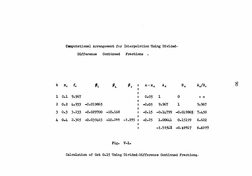
C~puta.tional Arrangement for Interpolation UsingDivided-

Difference Continued Fractions •

k £1< '1 ,~ " AI( Bl( AK/BK

\0xI< : x-xI< 0

::

1 0.1 9.967 : 0.0; 1 0 --•..2 0.2 4.9.33 -0.019865 • -0.05 9.967 1 9.967..

:3 0.3 3.233 -0.029700 -10.168 .. -0.15 -0.14799 -o.01986S~' 7.450..

..·4 0.4 2.365 -0.039463 -lO.2H3 -l.~B3 : -0.25 1.00641 0.15199 6.622:.. -l.6f9~£ -o••e9~1 6.6r;9~..

Fig. V-l.

Calculation of Cot 0.15 Using Divided-Difference Continued Fractions~

•

91

The result is in error by seven units in the third decimal

place, due partly to the small number of defining points

and partly to the round-off error of the original data.

In the example, the near-linearity of ¢. suggests

linearly interpolating 16, LO.10, 0.15] from the table and

calculating f(O.15) from the relation

¢, [Xo, x] = x - %0

~

The computational layout of Fig. V-l is also convenient---,-.,,,',,- - ~ .~ .. "_., ..

for observing the effective~ of convergence, since this

method of interpolation does not guarantee convergence to

the function value either qUickly or at all. At least a,ym­

ptotic convergence may be expected for the first n approximants,

where n is usually much larger than the number of iterations

acceptable for a computer subroutine.

Hildebrand mentions that this interpolation method,

being a rational approximation, is especially useful in the

neighbourhood of points where f(x) increases without bound.

As in the case of polynomial interpolation, initial

convergence may be hastened by judicious ordering of the

abscissae. Ascending order is used for interpolating near

the beginning of a table, descending order for values near

the end and near the middle of a table abscissae are taken

in alternate order on either side of the interpolant. This

92

ordering tends to maximize the rate of initial convergence

and this is a desirable thing for computer iteration but it)

does not improve ultimate convergence.

Several other considerations affect the suitability o~ The i.4~&'­

of inverted divided·difference continued fractions as an

interpolation method in a computer subroutine. Reference to

the computational arrangement of Fig. V-I shows that-;suecessive

inverted differences must be calculated at each step before

the next approximant is evaluated. Now the interpolant may

occur at any point within the range of available tabular

values,so that all inverted differences for the range should

be calculated beforehand. The method then appears most

suited to evaluating a fixed number of iterations for any

interpolant.

Much testing and calculating is necessary to set this

method up for a computer subroutine, that i~ to determine

the available accuracy of an approximant over the whole range

of the function. The initial tabular data may be accurate

only to the round-off error determined by the particular

machine. Results will be somewhat less accurate from this

Cause. If the round-off error of the machine is not fixed,

extra significant digits may be carried. The accuracy

desired (or possible) now determines the earliest approximant

-which will provide this accuracy over the whole range of

tabular values available to the machine. This in turn

93

determines the number of abscissae required in the table.

These abscissae and the partial denominators are fixed

constants for the subroutine. Calculation of partial

nwnerators of the form x - x k will usually take longer

than calculation of a single power of x, and is even more

inefficient if compared to a method in which a partial

numerator, once calculated, is used for all iterations of

the process.

These considerations indicate that a slow-running

subroutine will result from the use of continued fractions

as an interpolation method to calculate function values.

94

VI CONVERGENCE OF FRACTIONS TRANSFOmv~D FROM SERIES

Continued-fraction representations of some functions

were derived,in the last chapte~from their series expansion.

In this chapter the approximants will be examined to see

how they fit the function and etdr~ range over which they may

conveniently be used_ This will be done using the limits

on the error of an approximant given by (11-22) and the fact

that the approximants are rational functions. This examination

will cover the three functions whose continued-fraction

representation showed most promise for subroutines, namely

exponential, tangent and hyperbolic tangent.

1. The Exponential Function.

The first few approximants of the even part of the

continued fraction for eX are as follows.

1 ,1

2 +x ,T=X

:J •.. .. %" .. 2.. 2. 3

2 - 3•5 + 2 -.3 - 5x + 2 -.3x +x ,) . 2%. t t. 32 -)-; - -)-.5x + 2 .3x - x",. . :3 . . . . . 2.. .. .2. .2; ... . .• 3 . ..,.

2 -;-5-7+ 2 -3·5-7x+2 -,-% + 2 -5x + x ,If . j a. ~ t. . :3 If

2 - 3 -5 -7 - 2 •3 - ; -7x + 2 - 5.·9x - 2 .;x + Xfj" . 'I ••... ·tr·· .. . .J.. 2..) ..••.... If !/'

2 -:3 -·5 •7 •9 + 2 •3 -; -7 •9x + 2 .3 -5 .7x + 2.3 -5 -7x + 2 -3 •5x + x •1-3- ;-7-9 -i'-)- 5-7- 9x+ Z-3 -5·7r - t-3 -5 -7r- + 2-)·5x'" -x~

95

The following interesting poipts may be noted. The

numerator A~(x) is a polynomial of degree n having all signs

positive and no zero coefficients. The corresponding

denominator B~ (x ) : A'rI,(;';'x), so that the signs of odd power-s

of x are reversed. This property is sho~m to be true for

all approximants by using induction and the recurrence (II-6).

Approximants thus become their own reciprocal when x changes

sign. They agree in this respect with eX, the function

which they are approximating.

Now for x =0, each approximant has the value 1 and slope

1, thus agreeing with the function both in value and direction

at this fixed point. This property may be extended from the

approximants shown by using the recurrence relation and

induction, as well as by using the facts that any rational

ftmction of the form

y =a + bx +cx~ +-dx~+ • • •a ~ bx +- cx a - dx ~ +- • • •

(VI-l)

has the derivative --!!Ldx

o= 2b

aand that the ratio

alb = 2 for every approximant of eX.

For large values of I xl even approximants approach 1

asymptotically and odd approximants approach -1 asymptotically.

Even approximants approach from above for x positive, from

below for x negative. Odd approximants approach from below

for x positive"from above for x negative.

96

The first few approximants will now be examined

individually. Fig. VI-l shows the graphs of the oth, 1s t

and 2nd approximants superposed on that of eX. The graphs

of odd approximants resemble each other as do those of the

even approximants; therefore graphs of approximants following

the second have been omitted for clarity.

The zeroth approximant is identically one.

The first approximant has a vertical asymptote at

x - 2, is concave up~~rd and always-increasing for x less than

2 and is concave downward and always-increasing

than 2. It has one horizontal asymptote at y =for x greater

1. A real

root at' x = -2 is symmetric vTith regard to the origin to the

intersection with the x-axis of the vertical asymptote.

The second approximant is an increasing function from

the mt.ni.mum at x =-2{3 to the maximum at x =2/3, a decreasing

function elsewhere. It has one horizontal asymptote at y =1.

There are no vertical asymptotes. Inflection points are near

x =-6.9, 2.4 and 4.4. Concavity is upward between inflection

points near x = -6.9 and 2.4. The graph is always positive.

The graph of the third approximant resembles that of the

first, ~Tith a vertical asymptote near x =4.6 and a real

root near x =-4.6.

The graph of the fourth approximant is much like that of

the second. (The maximum is near x =6.10, the minimum near

x = -6.10. Inflection points occur near x =11.10, 3.39 and

97

<1" ,~t;

.--_..---..........-1:0 :

Fig. VI-l. ~raphs of

eX and Some of Its

Approximants in the

Neighbourhood of 2;ero.

o x

98

The graph of the fifth approximant has a single vertical

asymptote near x =7.29 and a real root near x =-7.29. It

resembles the graphs of the first and third approximants.

The graphs of the approximants can cut that of eX only

at (0,1). This is shown by the follo~rlng facts. Partial

quotients,after the first, are always positive. The maximum

error given by (II-22) changes sign only when x changes sign,

or when x crosses a'vertical asymptote. Formula (11-10)

shows that approximants are alternately greater than and less

than eX, at least for x to the left of the first vertical

asymptote for x positive.

The property of the approximants that they become their

own reciprocal when x changes sign shows that there is

symmetry about the origin between points of intersection of

vertical asymptotes with the x-axis and rea~ roots.

Differentiating (VI-6) yields a form having only even powers

of x in the numerator and a denominator which is square and

so non-negative. Thus horizontal tangents occur in pairs

whose abscissae are symmetric with respect to the origin and

whose ordinates are reciprocals. The second derivative shows

that one represents a maximum, th~ other a minimum.

Descartes' rule of signs shows that no approximant

has a positive real root, so there are no vertical asymptotes

for x negative. The nth approximant can have at most n

negative real roots and at most n vertical asymptotes for

99

x positive. If y is replaced by y - 1, it is seen that no

approximant crosses the line y =1 except at x =O.

The odd approximants thus form a sequence of functions

converging on eX from above "for x positive and to the left

of the first vertical asymptote for x positive, from below

for x negative. The even approximants are always positive

and converge on eX from below for x positive and from above

for x negative.

The following conjecture is offered, but could not be

proved. The odd approximants have one real root which is

negative and a vertical asymptote whose intersection with

the x-axis are symmetric with respect to the origin. They

are ever-increasing functions on either side of the asymptote.

The even approximants have one maximum and one minimum whose

abscissae are symmetric with respect to the origin. They

are increasing functions from the minimum to the maximum,

decreasing otherwise. Roots and asymptotes of succeeding

odd approximants and maxima and minima of succeeding even

approximants move farther apart.

Values of eX for x =0.1, 0.5, 1.0, 2.0, 3.0 and 5.0

listed in Table VI-l were computed on a lO-digit desk

calculator using the even part of the expansion.

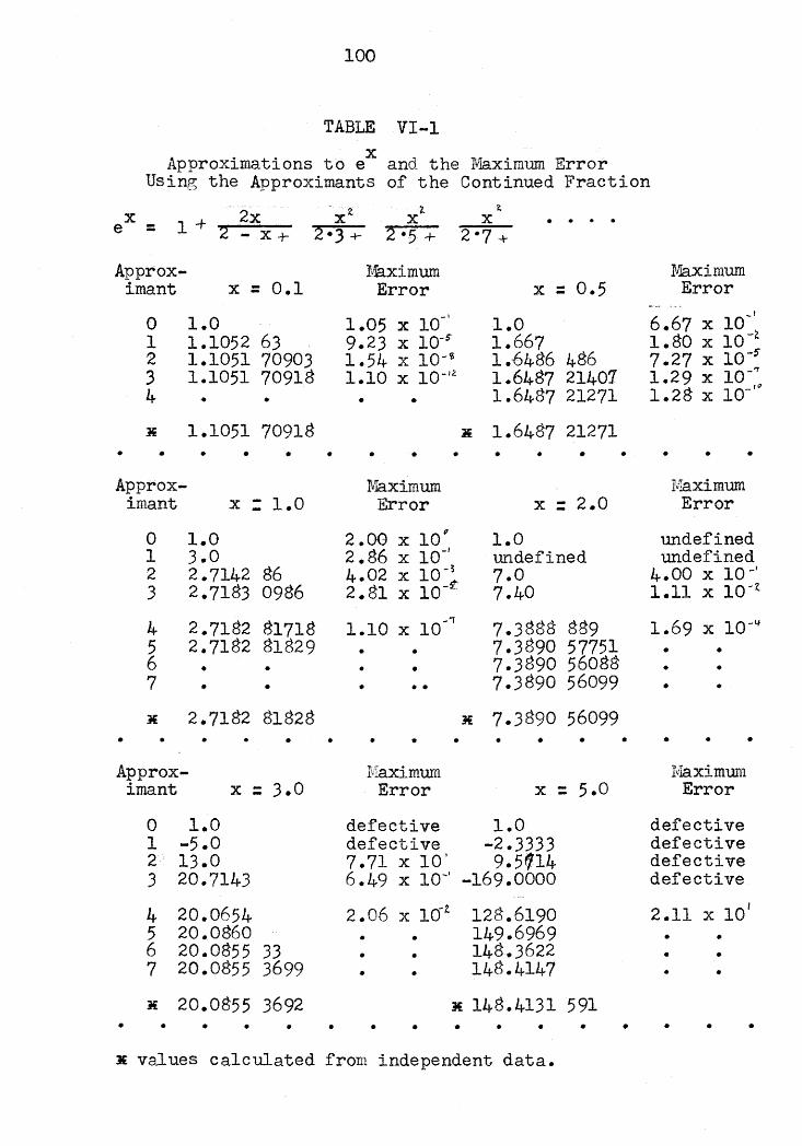
100

TABLE VI-l

Approximations to eX and the Ivlaximum ErrorUsing the Approximants of the Continued Fraction

eX = 1 + 2x2 - x +

. . . .Approx­

imant x =0.1IvBximumError x =0.5

N'.laximumError

o1-23q.

1.01.1052 631.1051 709031.1051 70918

• •

1.1051 70918

1.05 X 10-'9.23 X 10-5"1.54 x 10-~

1.10 X 10-12

• •

1.01.6671.6486 4861.6487 214011.6487 21271

li 1.6487 21271

....--'•..-'~

-'6.67 x 101.80 x 10-~7.27 X 10-5

1.29 X 10-'71.28 x 10-'"

• • • • • • • • • • • • • • • •

Approx­imant x : 1.0

f{aximumError x =2.0

IVIaximumError

• •

1.03.02.7142 862.7183 0986

2.7182 817182.7182 81829

•••

• •

• •• •

undefinedundefined

4.00 x 10-'1.11 x 10-~

1.69 X 10- 4

••••

1.0undefined7.07.40

7.3888 8897.3890 577517.3890 560887.3890 56099

]i 7.3890 56099•••

• •• • •

• •

-'11.10 x 10

•••

• •

•

o123

4567

•

Approx­imant x =3.0

NaximumError x = 5.0

MaximtllilError

o 1.01 -5.02 13.03 20.7143

4 20.06545 20.08606 20.0855 337 20.0855 3699

ii 20.0855 3692

defective 1.0defective -2.33337.71 x 10' 9.5q146.49 x 10-' -169.0000

2.06 x lcr t 128.6190• • 149.6969• • 148.3622• • 148.4147

i£ 148.4131 591

• •• •

•••

• •

I2.11 x 10

defectivedefectivedefectivedefective

•••••••••••••

x values calculated from independent data.

101

Some values of the maximum error given by (II-22i and

using the approximants as listed at the begiDning of this

section are listed beside the corresponding values of the

function. The value of eX calculated from l2-place tables

is listed as the value from independent data for each ar-gument ,

Each maximum error is only slightly greater than the

actual error. This suggests rapid convergence and suitability

for computer use. This is confirmed by the actual errors.

Maximum errors are listed as 'defective' when the argument

lies to the right of a zero of the denominator of (II-22);

These maximum errore are 'defective' in the sense that they

refer to the lower arm of the odd approximant concerned. The

first two maximum errors for x : 2 are undefined since they

have a zero term in the denominator.

The even part of the continued-fraction expansion of

eX was shovrn earlier to have a form well-suited to computer

calculation. It is now apparent that convergence is suffic­

iently rapid to keep rounding and truncation errors within

reasonable bounds. In programmin.g computer subroutines it is

common to restrict the domain of the argument so that excess­

ively-large function values are not generated. For instance,

the domain O<:x<:l is often used for eX. To evaluate

eX the integral portion of x is removed and the

102

fractional part evaluated by the subroutine. The final

function value is then obtained by multiplying by e the

number of times specified by the integral portion of x.

The fifth approximant yields ten figures of accuracy

for x within the above domain. The eighth approximant

yields ten figures of accuracy for the domain 0<:x<3.

For x negative the function may be found as the

reciprocal of that for x positive, or by using a negative

value, of x in the continued-fraction form. The equipment

of the computer being programmed and the use for which the

subroutine is intended will largely determine the domain

and method.

The Tangent Ftmction

The first faw approximants of tan x are as follows.

7- 5.-3:X: -5 -2:x: 3------ -- .,7. 5.; - 5-:3 -;% -I-X If

9-7-5.3x ~7-5.3x:1+ XS

,2nd ••

3r d ••

'*-th ••

;th ••

X tT,·)X

:3 - x1­:3

5·:3x- x5-3 - 3·2x~

,

,

6t h : 11.2·,·;-·3x....:9·'Z;;·4i3+'Z.jXS' •11- 9.7-; -3- 9-7.;. 5_;:X:2.+ 7-6-5x "l - x z

103

Succeeding approximants have the following properties

which may be deduced by using the recurrence relations (II-6)

and induction. The numerator A.".(x) is a polynomial of odd

degree (degree n for n odd, n-l for n even). All even

powers of x vanish but coefficients of odd powers of x are

never zero. The denominator B~ (x) is a polynomia~ of even

degree (degree n for n even, n-l for n odd). All odd powers

of x vanish but coefficients of even powers of x are never

zero. That is, numerators contain only odd powers of x,

denominators even powers. Each approximant adds one new term

to the polynomial either in the numerator or to that in the

denominator. The new terms are added alternately to the

numerator and to the denominator. Ih-·' theffpolynomials of both

numerator and denominator, the signs of the coefficients

alternate regularly, starting vnth the coefficient of x in

A~(x) and the absolute term of B~(x) positi¥e.

~_l approximants pass through the origin and have there

a slope of 1, as does tan x. All approximants are odd

functions and thus symmetric iflTith respect to the origin.

As x -> 00, odd approximants increase without bound in

the positive direction and become asymptotic to a straight

line of the form y =mx, where m decreases with successive

odd approximants. Even approximants have the x-axis for ~n

asymptote. In each case the asymptote is approached from

below as x increases, from above as x decreases.

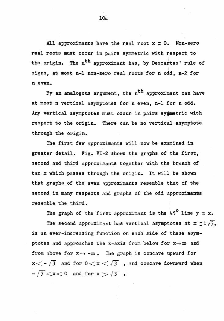
104

All approximants have the real root x =O. Non-zero

real roots must occur in pairs symmetric with respect to

the origin. The nth approximant has, by Desca~test rule of

signs, at most n-l non-zero real roots for n odd, n-2 for

11 even.

By an analogous argument, the nth approxi~ant can have

at most n vertical asymptotes for n even, n-l for n odd.

Any vertical asymptotes must occur in pairs sy_atric with

respect to the origin. There can be no vertical asymptote

through the origin.

The first few approximants will now be examined in

greater detail. Fig. VI-2 shows the graphs of the first,

second and third approximants together with the branch of

tan x which passes through the origin. It will be shown

that graphs of the even approximants resemble that of the

second in many respects and graphs of the odd approxi.an*s

resemble the third.

The graph of the first approximant is the 45° line y =x.

The second approximant has vertical asymptotes at x :! 13,is an ever-increasing function on each side of these asym­

ptotes and approaches the x-axis from below for X~CD and

from above for x~ -00. The graph is concave upward for

x< - f3 and for 0 < x < 13 , and concave dQwnward when

- IT<x< 0 and for x > f3 •

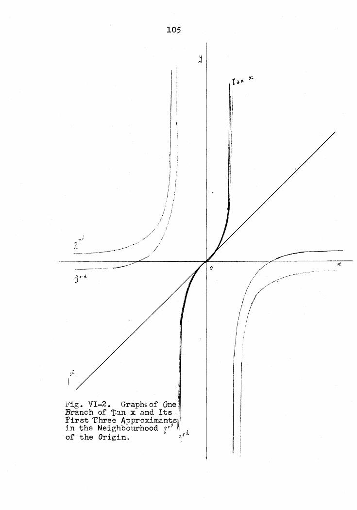
105

z

!II

Fig. VI-2. Graphsof OnelBranch of Tan x and Its iFirst Three Approximan~sjin the Neighbourhood Zf". I d.of the Origin.. ~ r

106

The third approximant is also an ever-increasing function

between discontinuities. lBetween its vertical asymptotes it

resembles the second approximant. The asymptotes have moved

in to x = ~ ,/10. The asymptote y =x/6 replaces the x-axis

as a non-vertieal asymptote. Non-zero real roots appear

at x =! )15.

The fourth approximant has two pairs of vertical asymptotes

near x = ! 1.571 and: 6.522. A pair of real roots are at

x = ! iJ42. Beyond the outer pair of vertical asymptotes

the graph becomes asymptotic to the x-axis in a manner

resembling that of the second approximant.

The fifth approximant, like the fourth, has two pairs

of vertical asymptotes, near x - ± 1.571 and ~ 5.053. Non­

zero real roots occur near x = !3.l53 and ~9.750. The non­

vertical asymptote is y : x/IS.

All partial numerators follolrlng the first are negative

and all partial denominators are positive, regardless of the

sign of x. The expression (IT-IO) for the difference between

successive approximants must therefore, for the first approx­

imants, have the same sign for a given x between the inmost

pair of vertical asymptotes of the n_lt h approximant (i.e.

when B"J\ and B~_, have the Same sign).

107

As a result,the expression (11-22) may not be used to evaluate

the maximum error involved in using a given approximant.

Now A~_J. _A", is always negative for x positive and positiveBY\"1 BI'\

for x negative, so the approximants are approaching the function

from below for x positive and from above for x negative,

at least between the inmost pair of asymptotes of tan x.

Thus the approximants are converging to the function from one

side rather than bracketing the function as in the case of eX.

(rhe inmost pair of vertical asymptotes of the approximants

appears to be converging on the value IT/2, as is to be

expected.

The series for sin x and cos x which were used to form

the continued fraction have infinite radit of convergence.

The infinite continued fraction may then be expected to

converge on tan x at least for all real x. In the limit it

will give vertical asymptotes at intervals of 11 starting

from 1f/2. and real roots at intervals of 11 starting from

the origin. The first faw approximants do begin to do this

in fact, at least to the extent permitted by the polynomials

in the numerators and denominators. An infinite continued

fraction would have an approximant whose numerator and

denominator 1A.Jl)L:ht bfJ-Dt infinite degree. ~flz(3fzJ. would provide the

requisite number (infinity) of vertical asymptotes and real

were and in which order they would occur.

108

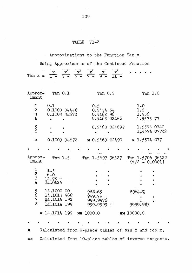
109

TABLE VI-2

Approximations to the Function Tan x

Using Approximants of the Continued Fraction

• • • • •

Approx­imant

1234

?6

Tan 0.1

0.10.1003 34~448

0.1003 34672• •

• •• •

0.1003 34672

Tan 0.5

0.50.5454 540.5462 960.5463 02465

0.5463 024898• •

* 0.5463 02490

Tan 1.0

1.01.51.5561.5573 77

1.5574 07401.5574 07722

1i 1.5574 077

• • • • • • • • • • • • • • •

Approx- Tan 1.5imant

Tan 1.5697 96327 Tan 1.5706 96321(11'/2 - 0.0001)

1 -1.5 • • • •2 6.0 •• • •3 12 6' ~, • • • •4 14:' 26 • • • •

5 14.1000 00 988.65 8964.cg6 14.1013 968 999.79 • •7 14.1014 191- 999.9976 • •8 14~lO14 199 999.9999 9999.983

:Ii 14.1014 199 ** 1000.0 }£JE 10000.0

• • • • • • • • • • • • • • •

* Calculated from 9-place tables of sin x and cos x.

~ Calculated from 10-place tables of inverse tangents.

110

The eighth approximant of tan x yields nine

figures of accuracy for x~ 1.5. It yields

tan 1.569796327 = 999.999953, \hThich differs from-6the tabulated value of 1000 by 5 x 10 • vfuen

x : 1.570696326, which is ~/2 - 0.0001 to nine places

of decimals, the eighth approximant yields tan x =_l.-

9999.983, which is in error by 2 x 10 of the tabulated

value of 10,000.

The expression (11-10) for the difference

between successive approximants yields, for x =1,

the f'o I'lowi.ng values.

Approximants Difference

2 - 1

3 - 2

4 - 3

5 - 4

6 - 5

5.00 x 10->

5.56 'x 10-~

1.82 x 10-~

-:i3.04 x 10

-~

3.15 x 10

These are all slightly.smaller than the actual errors.

This indicates a rapid convergence for the continued-

fraction expansion of the function.

The continued-fraction expansion of tan x is then

well-suited for use as a computer subroutine, since it has

both simple form and fast convergence to keep rounding errors

III

small. In practice a computer subroutine woul.d first reduce

the argument to the corresponding value in the doma±n

-1T/2<x <..Tr/2, evaluate for x positive and prefix the correct

sign. ~ince the end values of Z1T/2 are usually neglected

in tangent subr-outd.nej the d..~.(tl would be taken 0< x < 11/2 -f

where ( is determined by the characteristics of the computer

being programmed and the purpose of the program. Pracyical

accuracy may be attained for most computers by using th~

eighth approximant.

In preparing a subroutine to evaluate tan x, the

difference,as given by (11-10)., between successive approximants

will give a good indication of the order of magnitude of the

maximum error to be expected, but it should be checked by

actual calculation near the end of the doma~R of x.

3. The nyperbo1ic Tangent Function

'fhe continued-fraction expansion of the hyperbolic

tangent yields the following approximants.

1s t : X'1 '

,

,3:x:3+x.z.

5- 3x+ x 3

5-3 +3·2x%..3

7- 5.~ 3x + 5.2x ,

7~5-3 +9:5x'l.. + x "

112

9· 7 -5 •3 + 7·5 -4 •3x 2 + 5·3:x:JI.

~i·9·7·5 ·3x-r §e?-S·4X} + Z·3x' •

The terms of the polynomials in the numerators and in the

denominators of the approximants A~{x}/B~(x) are identical

with those of the corresponding approximants of tan x, but

have positive signs. Using the recurrence relations (11-6)

and induction, the follo~dng properties of the approximants

may be deduced.

A~(x) is a polynomial of degree n for n odd and degree

n-l for n even. Coefficients of odd powers of x never vanish,

while all coefficients of even powers of x always vanish.

B~(x) is a polynomial of degree n for n even and of degree

n-l for n odd. All even powers of x appear in the polynomial

while no odd powers of x ever appear. All signs are positive

in both A~(x) and in B~{x). Each approximant adds one new

term to either the polynomial in the numerator or to that in

the denominator. Ibis new term is added alternately to the

numerator and to the denominator starting ,nth the nlli~erator

of the zeroth approximant.

All approximants cross the x-axis at the origin and with

a slope of 1, as does the function they are approximating.

Each approximant is an odd function and thus s~etric with

respect to the origin.

113

As x ~+oo, the odd approximants increase 1ri thout bound

and are positive. They approach the same asymptote as does

the corresponding approximant of tan x but from the opposite

side. The even approximants approach the x-axis from above

as x-;>-+co. The behaviour as x ~ -00 is obvious by symmetry.

Descartes' rule of signs shows that there can be no

positive real roots and no vertical asymptotes for x positive.

S~nmetry of the approximants, or the application of Descartes'

rule of signs for x negative, indicates the absence of either

real roots or of vertical asymptotes for x negative. All

approximants have one real root at x : o.

Synunetry of the approximants indicates that maxima are

sywmetric to minima ,rith respect to the origin and that

inflection points must also occur in pairs symmetric with

respect to the origin.

Graphs of the first, second and third approximants,

superposed on that of tanh x for comparison, are drawn in

Fig. VI-3. Graphs of the second, fourth and sixth approx­

imants resemble each other closely as do those of the third

and fifth approximants, so graphs of approximants follovnng

the third have been omitted for clarity. S~rrmetry of the

graphs allo\ffl the discussion to be restricted to the case

of x posit.ive , Detailed discussion of the first fevl

approximants follows.

The first approximant is the 450 line y - x.

114

!

II

...", "..'...lt

115

The second approximant reaches a single maximum at

x = f3 . The graph is concave downward. for 0<x<3

and concave upward thereafter. The single positive inflect­

ion point is at x =3. The graph approaches the x-axis

asymptotically from above as x ~oo.

The third approximant is an ever-increasing function

having neither maxima nor minima. It is concave downward

from x =0 to the single inflection point near x =2.739,

ooncave upward thereafter. It approaches the asymptote

y : %/6 from abovevas x~ Q!:) •

The graph of the fourth approximant resembles that of

the second. It has a single maximum near x =3.0506. It

is concave downward from x =0 to the single inflection

point near x = 8.3010 thence concave upward as it approaches

the x-axis asymptotieallyfrom above.

The fifth approximant, like the third, is an. ever-increas­

ing function having neither maxima nor minima. It is concave

aownward from x =0 to the single inflection point near

x =3.916, thereafter concave upward. It approaches the

asymptote y : x/15 from above in the same way that the third

approaches y : x/6.

All the partial numerators, after the first, and all the

partial denominators of the continued-fraction expansion of

tanh x are pOSitive for all values of x. Relation (II-IO)

shows tha~ the difference between successive appreximants

116

must alternate in si.gn so that for x positive even approx­

imants converge on the function from below while odd app­

roximants converge on the function from above. The reverse

holds true for x negative as the approximants are odd

functions. The expression (1I-22) is thus applicable in

estimating the error in using an approximant.

Table VI-3 lists values of successive approximants for

x =O.i, 0.5, 1.0, 2.0, 3.0 and 5.0, together with the

corresponding maxa.mum error calculated from (11-22). Tanh x

for the same arguments was also computed from nine-place

tables of hyperbolic sin x and hyperbolic cos x and is

tabulated for reference. It may be noted that the estimates

of error calculated from (11-22) are correct to two or three

significant figures for arguments up to 2.0 and even there­

after approximate the error reasonably~well. Convergence,

then, is quite good in the vicinity of the origin, the eighth

approximant giving nine significant figures of accuracy up

to about tanh 1.5.

All approximants except the first are concave downward

to the right of the inflection point at the origin. Relation

(11-10) shows that no approximants cross tanh x or each other

except at the origin. It f'oLLows that odd approximants

must have at least one inflection point for x positive or c~oss

117

TABLE VI-3

Approximations to Tanh x and the I'}Iaximum ErrorUsing Approximants of the Continued Fraction

• •

Approx- Tanh 0.1imant

I~t9ximtU11

ErrorTanh 0.5 IvIaximum

Error

~ 0.0996 679946

12345

0.10.0996677740.0996 679947

• •• • •

0~5 3.85 x 10-~0,4615 38 5.83 x 10-4

0.4621 2121 4.07 x 10-:0.4621 17141 1.60 x 10-

-II

0.4621 17157 4.01 x 10

* 0.4621 17157• • • • • • • • • • • • •

Approx- Tanh 1.0imant

MaximumError

Tanh 2.0 NiaximumError

J. 0.7615 94157

1234

-567

1.00.750.7619 050.7615 8940

0.7615 942030.7615 94156

• •

-,2.50 x 10_~

1.19 x 10-t.J

3.15 x 10 ,4.80 x 10-

4.73 x 10-g

• ••

2.00.8570.97430.9634 55

0.9640 4890.9640 27020.9640 2769

* 0.9640 27580

1.14 x 10:,1.17 x 10_~

1.09 x 105.94 X 10- 4

-~2.18 x 10• ••

• • • • • • • • • •

Approx- Tanh 3.0imant

1 3.02 0.753 1.04354 0.9898 55 0.9954 $4

6 0.9950 327 0.9950 5569'8 0.9950 547239 O'~995054754

* 0.9950 54753

Maximllil1Error

• •• •• •• •

Tanh 5.0

5.00.53~ •1.21210.95691.0074 4

0.9989 31.0000 0980.9999 00940.9999 09759

if 0.9999 09204

Max'imumError

,4.4:6 x 106.76 X 10-

1

-,2 •.55 x 10_~5.06 x 108.52 x 10-'

• •• •• •• •

~ Values calculated from 9-place tables of sinh x and cosh x.

118

the even approximants asymptotic to the x-axis. It is

conjectured that odd approximants have only one inflection

point for x positive. Similarly the even approximants

must have at least one maximum for x positive and one

inflection point beyond the first maximum,since they are

asymptotic to the x-axis. It is again conjectured that

evenapproximants have only one maximum and one inflection

point for x positive.

The continued-fraction expansion of tanh x is then

admirably suited to produce approximations in a computer

subroutine, since it combines rapid convergence with simple

form. In practice it would be necessary to limit the ~om~tn

of the argument to the smallest value at which tanh x differs

from 1.0 by the round-off error of the machine. For values

outside this <nnttcll'!f1 the subroutine woul.d automatically

evaluate the function as + 1 or -1 according to the sign

of the argument.

4. Some Observations on !hese Continued Fraction Representation~

Tan x has a series expansion whose terms are positive,

that is to sa~ each term added causes the series to converge

to the function from below for x positive and less than TI/2.This is also true of its continued-fraction expansion,which was

derived from the same series for sin x and cos x.

Similarly tanh x has an alternating series expansion

and a continued-fraction expansion both of which bracket the

119

function as successive terms or partial quotients are added.

The exponential function, however, has a positive series

expansion while the approximants of its continued-fraction

expansion are alternately~essLand'.greateE"than the function

when x is positive. This counter-example shows there is no

simple connection between the behaviour of the two forms of

expansion although they may be equivalent in some respects.

The graphs of successive approximants of the three

functions considered not only approach more closely the graph

of the function, but imitate its behaviour over a greater

domain of the argument. It would be desirable then to define

an "effective domain of convergence" for each approximant.

Within this domain the approximant should behave reasonably­

like the function it is approximating, while beyond this

domain it rapidly deteriorates in its attempt to Simulate

the form of the function.

An effective domain of convergence for the even

approximants of eX might be taken to be between the first

minimum to the left of the origin and the first inflection

point or first maximum to the right of the origin. For odd

approximants the domain could be taken from the first real

root to the left of the origin to the first vertical

asymptote to the right of the origin.

An effective domain for approximants of tan x is limited

by the function to the interval -1T/2 <x < W2.

120

Even approximants of tanh x begin to diverge from the

function quite rapidly outside the domain between the first

minimum to the left of the origin and the first maximum to

the right. Odd approximants follow the form of tanh x between

the pair of inflection points nearest the origin but diverge

from tanh x quite rapidly outside this domain. A domain

between the points where the odd approximants cut the lines

y =+1 (the horizontal asymptotes of tanh x) might be more

suitable for some purposes.

This variety of possible criteria to determine a domain

of convergence for merely three functions, plus the fact

that different criteria may be applied to different approximants

of the same function, indicate the difficulty in defining a

single criterion to d~~A~~ a domain of convergence which would

apply for all approximants of all continued-fraction expansions

of all functions. Nevertheless the concept of a domain

within which an approximant behaves reasonably-like the

function it is approximating and beyond which it deteriorates,

is a valuable one for the preparation of a computer subroutine

using continued~fractionexpansions. It has the practical

effect of warning the programmer that any working domain

chosen must fall within a suitable domain for the approximant

used. It also warns 6.f"w'h'el1 .a chosen working domain may f al.L

outSide the effective domain of convergence of earlier

appr-oxtmants , If overlooked, this latter occurence can

121

cause difficulty when evaluating successive approximants

to attain a predetermined degree of accuracy.

\\ihen a fixed number of partial quotients are used, two

schemes of evaluation are possible. One scheme evaluates

the continued fraction form beginning at the ultimate partial

quotient, the other evaluates the rational form of the corres­

ponding approximant. The method requiring least time on the

computer being progra~ned will be the one usually chosen.

However, in some cases, such as tan x for 1.5 <X<1r/ 2 ,

fairly large function values are generated using a small

divisor and a large dividend. A check of relative errors

in the dividends and divisors is required to choose the more

accurate method.

It may also be noted that the similarity between the

continued-fraction expansions of tan x and tanh x would permit

a common subroutine to evaluate either function. The choice

of function would be by the point of entry into the program,

as is often done for sine-eosine subroutines. Such a

subroutine cOlud be auite useful for some applications.

122

VII CONVERGENCE OF CONTINUED FRACTIONS FORIvlED FROrvI

INVERTED DIVIDED DIFFERENCES

The method of interpolation using continued fractions

described in chapter IV may be used to interpolate tabulated

values of a known analytic function or to tabula~ values whose

anal.vt Lc form is unknown, ffhe rational function defined by

such an approximant is formed 51) as fb::pASb through the fixed

tabular points rather than to simulate the function. The

error involved in using the rational function may be made as

small as desired by choosing a sufficiently large number of

tabular points (using a later approximant).

This interpolation method has been used to compute values

of tan x bi .-tht:lt~SsfijfJ different numbers of equidistant abscissae.

Four, six and eleven abscissae permit the use of third, fifth

and tenth approximants. the data for the three cases are

listed below,showing first the fixed points x k and the

corresponding partial denominators b~, followed by a second

list ahowi.ng the values of x tested together 1.nth the value

of tan x calculated using the continued fraction and the value

of tan x calculated from 9-place tables of sin x and cos x

and finally the magnitude of the error involved for the

value of x used.

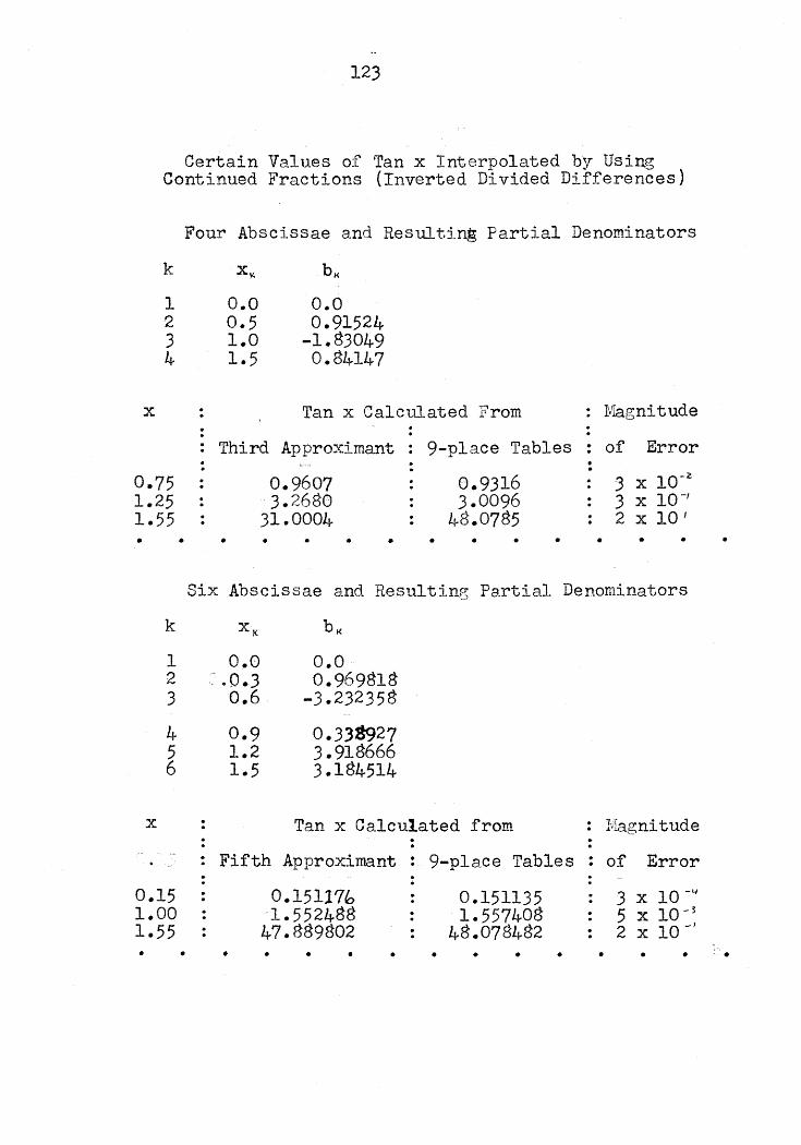
123

Certain Values of Tan x Interpolated by UsingContinued Fractions (Inverted Divided Differences)

Four Abscissae and Resulting Partial Denominators

k

1234

x

0.00.51.01.5

0.00.91524

-1.830490.84147

Tan x Calculated From Magnitude

Third Approximant 9-place Tables : of Error·· •.

0.75 0.9607 0.9316 3 x 10-'1.25 3.26s0 3.0096 3 x 10-'1.55 31.0004 48.0785 2 x 10 J

• • • • • • • • • • • • • •

Six Abscissae and Resulting Partial Denominators

· . .· . .

k

123

456

x ..·

0.0.. 0.30.6

0.91.21.5

0.00.969818

-3.232358

0.33S9273.9186663.184514

Tan x Calculated from Magnitude

: Fifth Approximant 9-place Tables of Error

0.151.001.55

·..·..··0.15117h1.552488

47.889802··

0.1511351.557408

48.078482

3 x 10-4

5 x 10-3

2 x 10- J

• • • • • • • • • • • • • • •

124

Eleven Abscissae and Resulting Partial Denominators

k

1234

'56

~9

1011

0.000.150.300.45

0.600.750.901.05

1.201.351.50

0.00.9924 88733

-6.6165 89090.0886 56164

6.9305 8584­5.2126 5441

-0.32-1+1 06275-1.1060 00610

-1.4.58g 992772.3282 49972.4669 4686

: Tenth Approximant; 9-place !ables

• • • • • • • • • • •

··

••

• Magnitude••.•· of Error··• 10- 7

• 2 x·· 1 x 10- f•· 4: x 10- c;

'" 6 x 10- ,•· 2 x 10- i'

1 x 10-,· 2 x 10- .,'"• 0·:• 4 x 10- ?•· 2 x 10- 7·· 8 x lO- s·

• • • •

0.0751 409420.1003 346720.255"3 419200.5463 02490

0.8004 249431.3983 825911.4749 625931.5574 07724-

3.2-e15 25858.2380 9278

48.0784 820••

••··•·

•·

•·

·•

·•

··•·

•·

Tan xCalculated from

0.0751 407530.1003 34664­0.2553 419240.5463 02496

0.8004 249301.3983 825901.4749 625951.5574 07724

3.2815 2;_t8.2380 9292

48.0784 027

••

•..•···

x

0.675 :0.9500.9751.000 :

1.2751.450 :1.550

0.075 :0.100 :0.250 :0.500 :

125

VIII

126

CONCLUSION

The aim of this thesis has been to examine the suitability

of continued fractions for approximating functions,

particularly in electronic-computer applications.

It has been found that continued-fraction expansions

compare favourably with series expansions for these purposes.

The methods seem to be complementary rather than competitive

since functions having awkward series expansions may have

tractable continued-fraction expansions and conversely.

Even when competitive, the different methods. may have

advantages for different computers depending on the equipment

available in the latter.

Some continued fractions have a regular form and also

converge sufficiently rapidly to be useful for computer­

subroutine applications. In many more cases the continued­

fraction expansion may be regular but convergence so slow that

hundreds or thousands of approximants may have to be evaluated

to attain a few decimals of accuracy. Contraction formulae

are usually of little benefit here since the number of partial

quotients to be abridged at each step and the point at which

to apply the contraction formulae to be used to produce a

reasonably-tractable form of continued fraction will usually

be 2Inat:tttrs' of trial and error.

127

One method of hastening the convergence of a slowly

converging continued fraction is given by P. W"ynn [18J '

who uses a converging factor technique. Essentially this

consists of replacing a sequence of partial quotients

beginning at some point in the continued-fraction expansion

by an approximation to the complete quotient from the same

point. The approximation to be used replaces the partial

quotients which would be required for a given accuracy.

The method used is to set up a difference equation involving

the complete quotient spanning a sequence of partial quotients

and to solve by a system of recursions this difference equation

for the approximation to the complete quotient. For eval­

uating 11/2, ''''ynn gives a numerical example whereby the sixth

converging factor gives approximately the same accuracy as'1

the 10 th approximant.

An interpolation method using continued fractions has

also been examined and found suitable for the use in

computer programs in some dase$~

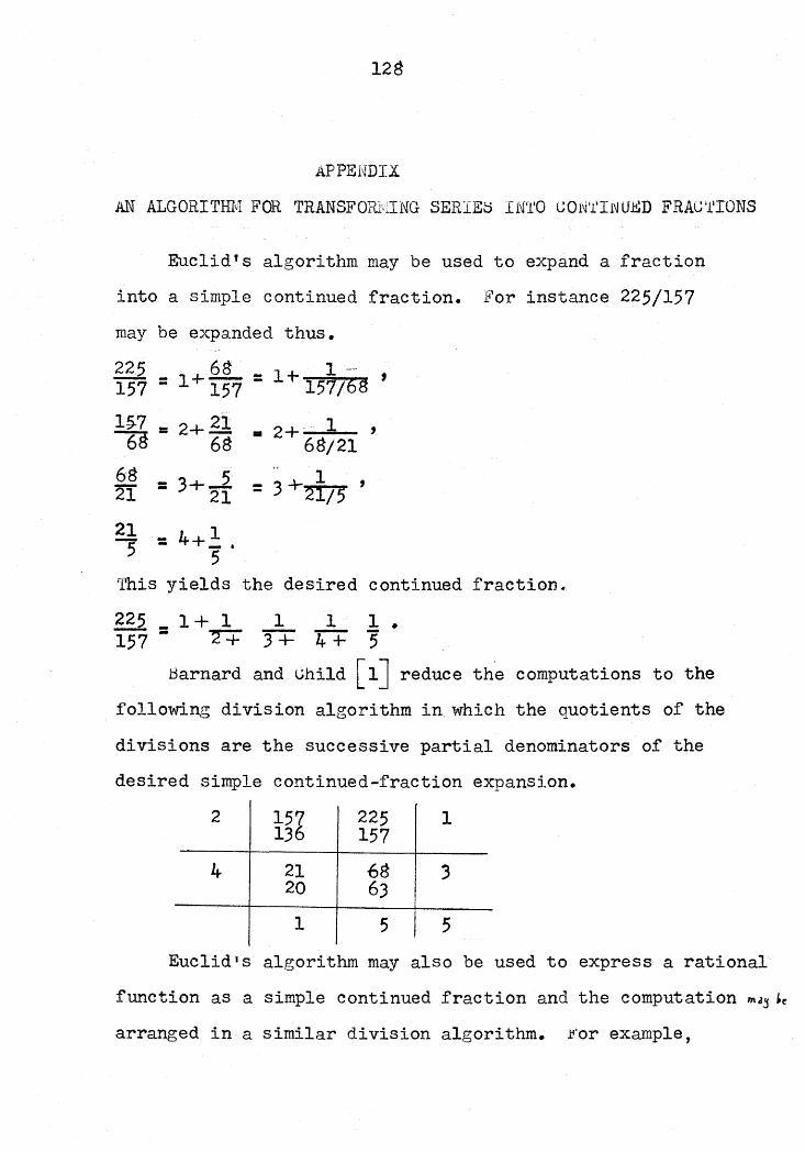
128

APPENDIX

AN ALGORITm~ FOR TRANSFORMING SERIES INTO CONTINUED FRACTIONS

Euclid's algorithm may be used to expand a fraction

into a simple continued fraction. For instance 225/157

may be expanded thus.

68 =1+ 157225157 =1~7 =6868 _2T -215" =

2+~68

3+-2.21

4+ 1- .5

1­1+ 157/68 '

• 2+. 1 ,68/21

=3+~'

This yields the desired continued fractionk

225 _ 1 + 1 1 1 1.157- ~ 3+ 4 + 5

Barnard and Uhi1d [lJ reduce the computations to the

following division algorithm in which the quotients of the

divisions are the successive partial denominators of the

desired simple continued-fraction expansion.

2 157 225136 157

4 21 6820 63

1 5

1

5

Euclid's algorithm may also be used to express a rational

function as a simple continued fraction and the computation Mdj 'earranged in a similar division algorithm. !i'or example,

129

1..

x/(1 - x} is expanded thus.

1 1 2x+x L- X x2x a. 1-3£ 2x 1.+ X

j

x-2

--2.... ~ +xL 2x

%. x 3 4x- - -- 32x .L 2JELZ! 2x2.

- -2 :3

X2. 3X X-:3 3

This corresponds to the following simple continued-

fraction form:.x _

(1- X)4 -x+ 1

1-2x2. +

1 1-Je -2

3 + 2x~ +--.l..

x:3

•

The partial denominators are again rational functions. ~his

simple continued-fraction form may be transformed to the

follo\rlng more convenient form:

x =x+ 2x4. ~ .?f.-- 2X••\1 _x)z 1 - 2 + 3 - 1

The simple continued-fraction form resulting from the

application of the division algorithm is not only awkward

to work with but tends to obscure any regularity of structure

which may develop in the partial quotients.

To avoid this difficulty and to obtain the continued­

fraction expansion directly in a convenient form, the

convention is made that the elements of the partial quotients

shall be of the formax~.

130

before proceeding \~th the division at any stage,

any power of x which can be taken out of the divisor as a

common factor becomes the partial numerator of the partial

quotient calculated at that step. Any integral common factor

may also be taken out of the divisor to simplify the form

of the continued-fraction expansion. the partial denominator

is then formed by division by the reduced diviso~ as in the

previous algorithm. the purpose of taking out the common

factor is made clear by comparing the step to the correspond-

ing quotient of ~uclidls algorithm. This revised algorithm

is used below to determine the partial quotients ofz,

xl (1- X)

2x%.-1

x-:3

directly.

1-2x+x~

I-x2

~1 - 2f2 :31"2

-.?f:3

xx-2~+ x 3

1 _ .!2

1 - '2:x:"3

x

-~2

-l!1

lbe partial numerator extracted as a common factor and

the partial denominator found by the division are written

as the full partial quotient at each step. The continued

fraction may then be written daVID immediately:

x _ x+2x~ k-i ~ _ -------

II - x) 1 - 2 +

131

x)-

2x1

•

The algorithm may be easily modified in a similar

manner to yield directly partial quotients whose partial

denominators are all unity.

1

3

5

6

7

132

WORKS CITED

S. Barnard and J. M. Child, Higher Algebra,1955, London, MacMillan and Co.,eu. 24., Ch. 33.

E. S.Barnesand H. P. F .SW'innerton-Dyer,"The Inhomogeneous :Minima of BinaryQuadratic "Forms", Parts I, II, III, IV,Acta Math., Vol. 87(1952~l, pp. 259-323',Vol. 88(1952), pp. 279-316, Vol. 92(1954.),pp. 199-234, 235-264.

Anunoy Chatterjee, "On a Continued Fr~etion

of .. a General .. Type" t Bull. Calcutta 1<1ath.Soo. Vol. l;.O(1948J, pp. 69-75.Reviewed in Math. Reviews, Vol. 10(1949),p. 246, reviewed by E. Frank (Chicago).

Julian Lowe.II Coolidge, The Mathematics ofGreat Amateurs, 1949, Oxford, The ClarendonPress, Ch. 11. .

Tobias Dantzig, The Bequest of the Greeks,1955, London, George Allen and Unwin Ltd.

H. Davenport, The Higher Arithmetic, 1904,London, Hutchinson t S IJifiyersity Library,ca. 4.

J. W. L. Glaisher, ffNumerieal Values ofCertain Continued Fractions", QuarterlyJour. Math., Vol. 13(1875), pp.255-259.

Library ofCongress

CatalogueNumber

QA154­125

QA1A18

QA1Iflv28

QA.2-8C69

QA22D19

QA1Ql

133

g H. Hamburger, "ftber Eine Erweiterung des QAStieltjesschen MomentprQb1ems", 1Parts I, II, III, Math. Ann., Vol. 81'(1920), M42pp. 235-319, Vol. 82(1920), pp. 120-164,pp. 168-187.

9 F. B.Hildebrand,-~ Introduction to Numerical ~A·

Analysis, 1956, New York, McGraw-Hill 300Book ce., Ch. s. H64

10 Walter Leighton, ·Proper Continued Fractions", QAAmer. :Math. Monthly, Vol. 4.7(1940), l'pp. 274-280. A5l

11 Adam Puig, "On Some Properties of ContinuedFractions of Differential'Elements"lLas Ciencias, Vol. 20(1955), pp. 499-309,Reviewed in rJIath. Reviews, Vol. 17(1956) .p. 1080, reviewed by H. S. Wall (Austin, Tex).

QA114428

12 W. T. Scott and a.S.Wall, "Continued Fractions", QANational l\rlathematics Iviagazine, Vol. 13 1(1938-39), pp. 305-322. M44

13 David Eugene Smith,Vol. II, 1925,

History of Mathematics,Boston, Ginn and Co.

14 T. J.Stie1tjes, "Recherches sur les Q.A.Fractiones Continues", Oeuvres, Vol. 2, 3pp. 402-566. S85

15 E. B. VanVleck, "On an EXtension of the QA1894 Memoir of Stieltjes·, Trans. !mer. 1Math. Soc., Vol 4(1903), PP. 297-332 A52

134

17 H. S. Wall j Analytic Theory of ContinuedFractions L 1948, New York, D. VanNostrand Go.

18 P. Wynn, ftConverging Factors for ContinuedFractions"', NumerisChe Mathematik,Vol. 1(1959), pp. 272-320.

QA1L8

QA'295W18

QA1